Motif statistics of artificially evolved and biological networks

Burcin Danacı1, Mehmet Ali Anıl2 and Ayse Erzan1

1Department of Physics Engineering,Istanbul Technical University, Maslak, Istanbul, Turkey2Department of Physics, University of Colorado, Boulder, Colorado, USA

(Dated: June 24, 2014)

Topological features of gene regulatory networks can be successfully reproduced by a model pop-ulation evolving under selection for short dynamical attractors. The evolved population of networksexhibit motif statistics, summarized by significance profiles, which closely match those of E. coli,S. cerevsiae and B. subtilis, in such features as the excess of linear motifs and feed-forward loops,and deficiency of feedback loops. The slow relaxation to stasis is a hallmark of a rugged fitnesslandscape, with independently evolving populations exploring distinct valleys strongly differing innetwork properties.

PACS Nos. 87.10.Vg, 87.18.Cf, 87.18.Vf

I. INTRODUCTION

Dynamical biological networks, such as gene regula-tory networks (GRN) have been the subject of intensivestudy over more than thirty years [1–8]. It is generallyagreed that topology is the main determinant of the dy-namical behavior. Milo et al. [9] have introduced theuseful concept of network motifs, and shown the pre-dominance of feed-forward loops in biological contexts.The significance profiles of the motif composition of sev-eral transcriptional GRNs reveal a marked enhancementof feed-forward loops and an equally marked absence offeed-back loops [10] (also see Klemm and Bornholdt [11].)

The viability or usefulness of biologically meaningfulregulatory networks usually require the dynamics to havea point attractor [12, 13], or a small number of multista-tionary states [2, 14–17]. This is easy to understand e.g.,in the context of tissue differentiation, where an embry-onic cell is once and for all committed to a particulartissue type, or within the context of periodic behaviorsuch as the diurnal cycle.

In this study, which builds upon and extends previouswork [18], we show that simply adopting a fitness func-tion which favors short attractor lengths (point attrac-tors and two-cycles) is sufficient to evolve, via a geneticalgorithm [19], populations of regulatory networks withtopological properties found in real-life gene regulatorynetworks. The adjacency matrix of each random graphcan be considered as its “genotype.” The “phenotype”of the network is the set of its dynamical attractors. Theconnection between the wiring (the genotype) and thedynamics (the phenotype) is a subtle one, allowing manydifferent types of solutions. By considering many dif-ferent, independently evolving populations, we are ableto observe if interrelations exist between properties suchas the mean degree, the motif statistics and the averagelength and number of attractors.

The significance profiles of the motif frequencies of dif-ferent populations of evolved networks show a marked re-semblance to those found by Milo et al. [10] for real generegulatory networks. Our results are consistent with ear-lier findings that the number of feed back loops are sup-pressed [2, 11] while there is a relatively high frequency of

feed-forward loops [9] in biologically relevant regulatorynetworks.

The evolutionary paths followed by the different pop-ulations can be very different from each other, neverthe-less yielding the desired characteristic of short attrac-tors. This is an indication of a rugged fitness landscapewith divergent valleys (where the mean attractor lengthis minimized), and is reflected in the slow relaxation ofthe evolutionary process.

In Section 2 we outline our model. In Section 3 wepresent our simulation results. Section 4 provides a dis-cussion of our findings.

II. THE MODEL

Our model networks [18] consist of N nodes. Initialpopulations of random directed networks are generatedwith an initial connection probability p0. Each elementof the initial adjacency matrix A, assumes values 1 withprobability p0 and 0 with a probability 1− p0 [21]. Thedirected edges connecting a pair of vertices (i, j) are as-signed independently of each other. Counting each di-rected edge separately, the total number of directed edgesis given by E =

∑ij Aij . The in- and out-degrees of

each node are initially independent and distributed ac-cording to a Poisson distribution with the mean p0N , and〈E〉0 = 2p0N . On the other hand the total connectionprobability between any two vertices is p0(2− p0).

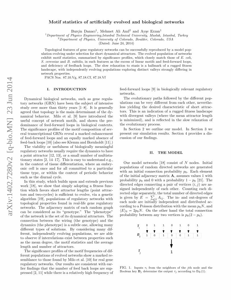
τi

Bij

τj

1 0 1 0 0 1 1

0 1 1 0 1 0 1

1

FIG. 1. Inputs τi from the neighbors of the jth node and theBoolean key Bj determine the output τj according to Eq.(1).

arX

iv:1

402.

7280

v2 [

q-bi

o.M

N]

23

Jun

2014

2

Variables τi, i = 1 . . . N which can take on the valuesof 1 or 0, correspond respectively, to an active or a pas-sive state of the node, as in the case of gene regulatorynetworks. The state of the system is given by the vectorτ .

The dynamics can be specified in two equivalent ways.We assigned a random vector, a Boolean “key” Bj =(B1j , . . . , Bij , . . . , BNj) to each jth node, with the en-tries taking the values 0 and 1 with equal probability.The nature of the interactions between pairs of nodesare thus predefined and mutations only affect the topol-ogy of the graphs by changing the adjacency matrices.All the networks have the same set of keys associatedwith their nodes. For each population, the keys are ran-domly generated once and for all in the beginning of thesimulations. While we change the wiring of the graphin the course of evolution, the keys have the convenientfunction of labeling the nodes.

The entries Bij = 0 or 1, correspond to an activatingor suppressing interaction respectively (see Table I). Thesynchronous updating is given by a majority rule,

τj(t+1) = ΘH

( N∑i

Aij

{[τi(t) XOR Bij ]−

1

2

}). (1)

The Heaviside step function is defined as

ΘH(x) =

{1 for x ≥ 0

0 for x < 0. (2)

If there are no incoming edges to the node, j, i.e., orkj =

∑iAij = 0, then τj(t+ 1) ≡ τj .

It is clear that the two states (active/silent) of a nodecan just as well be represented by Ising spins si = 2τi −1 = ±1. In this case it is convenient to think of theset of Boolean vectors Bj as an interaction matrix andto define σij = 2Bij − 1 = ±1, with ±1 correspondingrespectively to an activating or suppressing interaction.The input si = ±1 from the ith node to the jth node isthen processed using σij , and the update rule becomes,for kj 6= 0,

sj(t+ 1) ≡ 2ΘH

(N∑i

Aijσijsi(t)

)− 1 . (3)

The model is then equivalent to a finite diluted spin glass.This representation also allows us to make direct contactwith the work of Thomas and co-workers [2, 14–16]. Notethat an activating (+) interaction means that, if the acti-vating gene is on (i.e., it has the value 1) then it will con-tribute towards turning the target gene on; conversely, ifthe activator is off (i.e., has the value 0), this will tendto turn off the target gene. The complement is true forthe repressive (-) interaction; if a repressor is on, this willcontribute towards silencing the target gene, but if therepressor is off, then this will contribute towards turningthe target gene on.

TABLE I. State table for the Boolean keys shown in Fig.1.The Bij are the elements of the “key” associated with the j’thnode, and τi indicates the state of the ith node. The outputof the jth node is computed via a majority rule ( see Eq.(1 orequivalently, (3)), where we count only the input from nodesconnected to j by a directed bond. This condition is ensuredby the factor Aij , which is unity if there exists a bond (i, j)and is zero otherwise.

Input Key Output Interaction

τi Bij τiXOR Bij type σij

0 0 0 activating +

1 0 1 activating +

0 1 1 repressing -

1 1 0 repressing -

The population of networks is evolved using a geneticalgorithm [19]. The codes used for the simulations can beaccessed from [20]. We have chosen the fitness function todepend on the mean attractor length, a, of the network,averaged over the whole phase space, i.e., all possibleinitial conditions, so that each attractor is weighted bythe size of its basin of attraction. The fitness functionf(a) favors average attractor lengths a ≤ 2. Selectednetworks are cloned and then mutated by rewiring theedges, while preserving the in- and out-degrees of eachnode.

The steps of the genetic algorithm are as follows:1) Generate a population consisting of randomly wired

Boolean graphs, with randomly generated Boolean keysas described above.

2) Select the graphs to be cloned according to the fit-ness function f(a) = P for a ≤ 2, 0 otherwise. The valueof P = 1/2 was chosen for rapid convergence.

3) Mutate the clones, by randomly choosing two in-dependent pairs of connected nodes and switching theterminals of the two directed edges. This preserves thein- and out-degrees of each node.

4) Remove an equal number of randomly chosengraphs.

5) Go back to step 2.

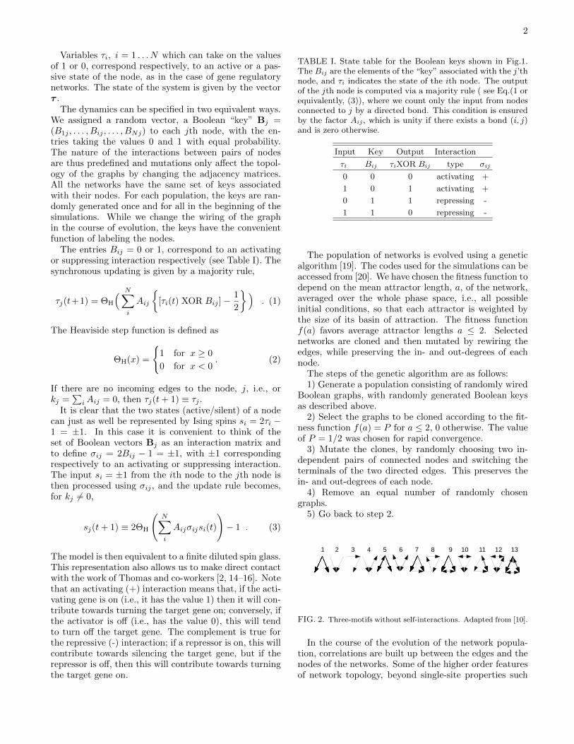
1 2 3 4 5 6 7 8 9 10 11 12 13

FIG. 2. Three-motifs without self-interactions. Adapted from [10].

In the course of the evolution of the network popula-tion, correlations are built up between the edges and thenodes of the networks. Some of the higher order featuresof network topology, beyond single-site properties such

3

as degree distributions, can be captured by the frequen-cies of common motif structures. Motifs are subgraphs ofnetworks, consisting of three or more connected nodes [9].Since our networks are small, we considered only 3-motifsand focused our attention on the interactions between thenodes by eliminating self-interactions. This yields a to-tal of 13 motifs shown in Fig. 2. To compare topologicalfeatures of the resulting graphs to those of randomizedgraphs, z-scores and significance profiles based on mo-tif frequencies were computed. The z-scores are definedas [9],

zµ =〈Nevol(µ)〉 − 〈Nrand(µ)〉

σ[Nrand(µ)](4)

where µ = 1, . . . , 13 is the motif label and 〈Nevol(µ)〉 and〈Nrand(µ)〉 are motif frequencies (evolved and random-ized, respectively) averaged over 103 graphs; σ[Nrand(µ)]is the standard deviation.

Significance profiles, S = (S1, . . . , Sµ, . . . , S13) for eachset of 103 graphs are obtained by normalizing the z-scores [10] to give,

Sµ = zµ

(∑µ

z2µ

)−1/2. (5)

It should be noted that in Ref. [10] the randomizationis carried out while keeping the degree sequence fixed,while we only keep the total number of edges fixed, dueto the randomizability problem we encounter with smallnetworks, as explained in the next section.

III. SIMULATIONS

A. Simulation procedure

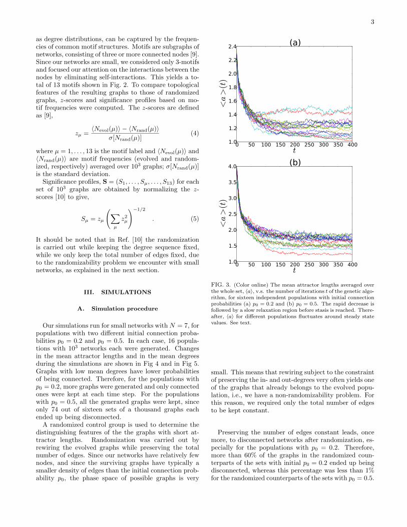
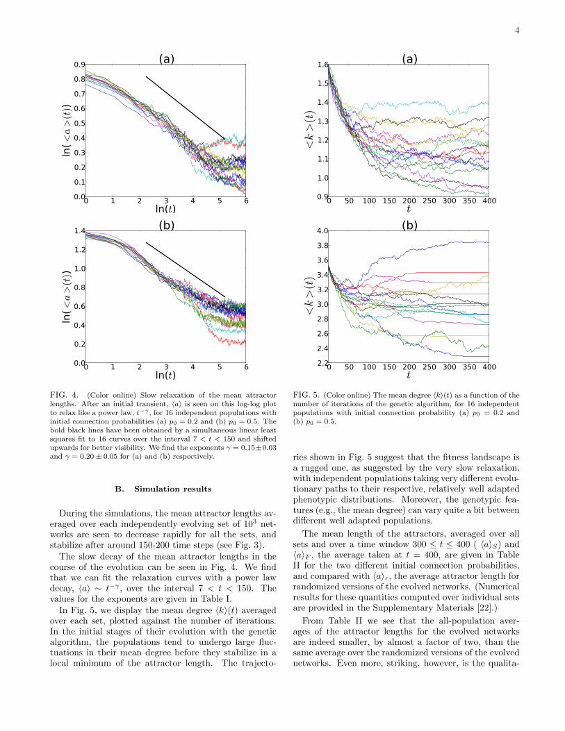
Our simulations run for small networks with N = 7, forpopulations with two different initial connection proba-bilities p0 = 0.2 and p0 = 0.5. In each case, 16 popula-tions with 103 networks each were generated. Changesin the mean attractor lengths and in the mean degreesduring the simulations are shown in Fig 4 and in Fig 5.Graphs with low mean degrees have lower probabilitiesof being connected. Therefore, for the populations withp0 = 0.2, more graphs were generated and only connectedones were kept at each time step. For the populationswith p0 = 0.5, all the generated graphs were kept, sinceonly 74 out of sixteen sets of a thousand graphs eachended up being disconnected.

A randomized control group is used to determine thedistinguishing features of the the graphs with short at-tractor lengths. Randomization was carried out byrewiring the evolved graphs while preserving the totalnumber of edges. Since our networks have relatively fewnodes, and since the surviving graphs have typically asmaller density of edges than the initial connection prob-ability p0, the phase space of possible graphs is very

0 50 100 150 200 250 300 350 400t

1.0

1.2

1.4

1.6

1.8

2.0

2.2

2.4

<a>

(t)

(a)

0 50 100 150 200 250 300 350 400t

1.0

1.5

2.0

2.5

3.0

3.5

4.0

<a>

(t)

(b)

FIG. 3. (Color online) The mean attractor lengths averaged overthe whole set, 〈a〉, v.s. the number of iterations t of the genetic algo-rithm, for sixteen independent populations with initial connectionprobabilities (a) p0 = 0.2 and (b) p0 = 0.5. The rapid decrease isfollowed by a slow relaxation region before stasis is reached. There-after, 〈a〉 for different populations fluctuates around steady statevalues. See text.

small. This means that rewiring subject to the constraintof preserving the in- and out-degrees very often yields oneof the graphs that already belongs to the evolved popu-lation, i.e., we have a non-randomizability problem. Forthis reason, we required only the total number of edgesto be kept constant.

Preserving the number of edges constant leads, oncemore, to disconnected networks after randomization, es-pecially for the populations with p0 = 0.2. Therefore,more than 60% of the graphs in the randomized coun-terparts of the sets with initial p0 = 0.2 ended up beingdisconnected, whereas this percentage was less than 1%for the randomized counterparts of the sets with p0 = 0.5.

4

0 1 2 3 4 5 6ln(t)

0.0

0.1

0.2

0.3

0.4

0.5

0.6

0.7

0.8

0.9ln

(<a>

(t))

(a)

0 1 2 3 4 5 6ln(t)

0.0

0.2

0.4

0.6

0.8

1.0

1.2

1.4

ln(<

a>

(t))

(b)

FIG. 4. (Color online) Slow relaxation of the mean attractorlengths. After an initial transient, 〈a〉 is seen on this log-log plotto relax like a power law, t−γ , for 16 independent populations withinitial connection probabilities (a) p0 = 0.2 and (b) p0 = 0.5. Thebold black lines have been obtained by a simultaneous linear leastsquares fit to 16 curves over the interval 7 < t < 150 and shiftedupwards for better visibility. We find the exponents γ = 0.15±0.03and γ = 0.20± 0.05 for (a) and (b) respectively.

B. Simulation results

During the simulations, the mean attractor lengths av-eraged over each independently evolving set of 103 net-works are seen to decrease rapidly for all the sets, andstabilize after around 150-200 time steps (see Fig. 3).

The slow decay of the mean attractor lengths in thecourse of the evolution can be seen in Fig. 4. We findthat we can fit the relaxation curves with a power lawdecay, 〈a〉 ∼ t−γ , over the interval 7 < t < 150. Thevalues for the exponents are given in Table I.

In Fig. 5, we display the mean degree 〈k〉(t) averagedover each set, plotted against the number of iterations.In the initial stages of their evolution with the geneticalgorithm, the populations tend to undergo large fluc-tuations in their mean degree before they stabilize in alocal minimum of the attractor length. The trajecto-

0 50 100 150 200 250 300 350 400t

0.9

1.0

1.1

1.2

1.3

1.4

1.5

1.6

<k>

(t)

(a)

0 50 100 150 200 250 300 350 400t

2.2

2.4

2.6

2.8

3.0

3.2

3.4

3.6

3.8

4.0

<k>

(t)

(b)

FIG. 5. (Color online) The mean degree 〈k〉(t) as a function of thenumber of iterations of the genetic algorithm, for 16 independentpopulations with initial connection probability (a) p0 = 0.2 and(b) p0 = 0.5.

ries shown in Fig. 5 suggest that the fitness landscape isa rugged one, as suggested by the very slow relaxation,with independent populations taking very different evolu-tionary paths to their respective, relatively well adaptedphenotypic distributions. Moreover, the genotypic fea-tures (e.g., the mean degree) can vary quite a bit betweendifferent well adapted populations.

The mean length of the attractors, averaged over allsets and over a time window 300 ≤ t ≤ 400 ( 〈a〉S) and〈a〉F , the average taken at t = 400, are given in TableII for the two different initial connection probabilities,and compared with 〈a〉r, the average attractor length forrandomized versions of the evolved networks. (Numericalresults for these quantities computed over individual setsare provided in the Supplementary Materials [22].)

From Table II we see that the all-population aver-ages of the attractor lengths for the evolved networksare indeed smaller, by almost a factor of two, than thesame average over the randomized versions of the evolvednetworks. Even more, striking, however, is the qualita-

5

2 4 6 8 10 12 14aF

0.0

0.1

0.2

0.3

0.4

0.5

0.6

0.7

0.8

0.9p(aF)

(a)

2 4 6 8 10 12 14aF

0.0

0.1

0.2

0.3

0.4

0.5

0.6

0.7

0.8

0.9

p(aF)

(b)

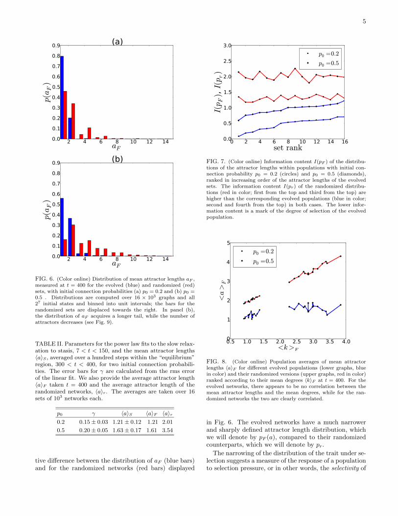
FIG. 6. (Color online) Distribution of mean attractor lengths aF ,measured at t = 400 for the evolved (blue) and randomized (red)sets, with initial connection probabilities (a) p0 = 0.2 and (b) p0 =0.5 . Distributions are computed over 16 × 103 graphs and all27 initial states and binned into unit intervals; the bars for therandomized sets are displaced towards the right. In panel (b),the distribution of aF acquires a longer tail, while the number ofattractors decreases (see Fig. 9).

TABLE II. Parameters for the power law fits to the slow relax-ation to stasis, 7 < t < 150, and the mean attractor lengths〈a〉S , averaged over a hundred steps within the “equilibrium”region, 300 < t < 400, for two initial connection probabili-ties. The error bars for γ are calculated from the rms errorof the linear fit. We also provide the average attractor length〈a〉F taken t = 400 and the average attractor length of therandomized networks, 〈a〉r. The averages are taken over 16sets of 103 networks each.

p0 γ 〈a〉S 〈a〉F 〈a〉r0.2 0.15± 0.03 1.21± 0.12 1.21 2.01

0.5 0.20± 0.05 1.63± 0.17 1.61 3.54

tive difference between the distribution of aF (blue bars)and for the randomized networks (red bars) displayed

0 2 4 6 8 10 12 14 16set rank

0.0

0.5

1.0

1.5

2.0

2.5

3.0

I(pF), I(pr)

p0 =0.2

p0 =0.5

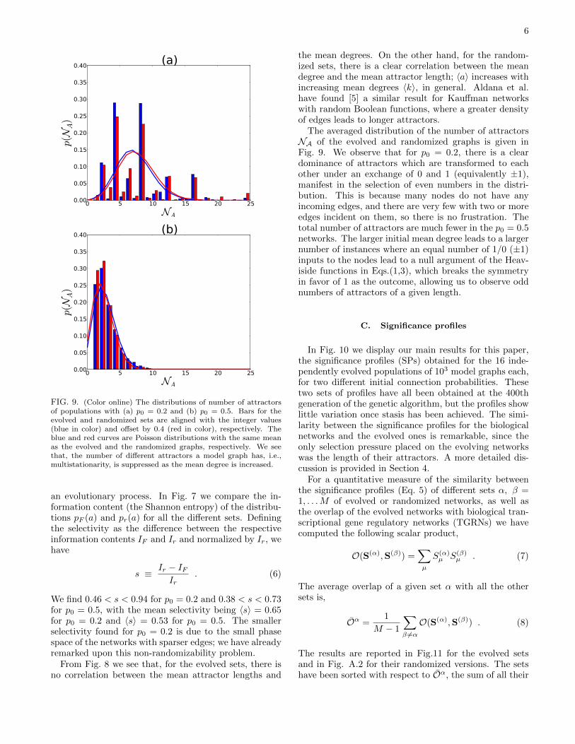
FIG. 7. (Color online) Information content I(pF ) of the distribu-tions of the attractor lengths within populations with initial con-nection probability p0 = 0.2 (circles) and p0 = 0.5 (diamonds),ranked in increasing order of the attractor lengths of the evolvedsets. The information content I(pr) of the randomized distribu-tions (red in color; first from the top and third from the top) arehigher than the corresponding evolved populations (blue in color;second and fourth from the top) in both cases. The lower infor-mation content is a mark of the degree of selection of the evolvedpopulation.

0.5 1.0 1.5 2.0 2.5 3.0 3.5 4.0<k>F

0

1

2

3

4

5

<a>F

p0 =0.2

p0 =0.5

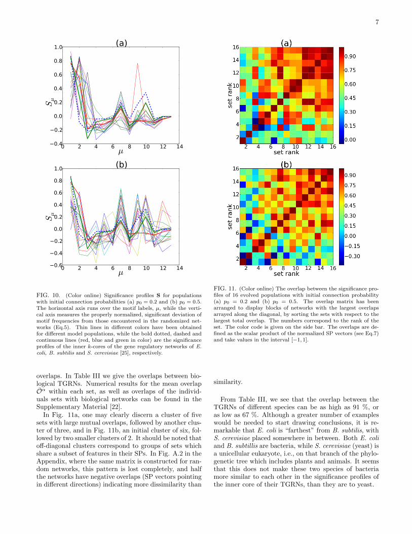
FIG. 8. (Color online) Population averages of mean attractorlengths 〈a〉F for different evolved populations (lower graphs, bluein color) and their randomized versions (upper graphs, red in color)ranked according to their mean degrees 〈k〉F at t = 400. For theevolved networks, there appears to be no correlation between themean attractor lengths and the mean degrees, while for the ran-domized networks the two are clearly correlated.

in Fig. 6. The evolved networks have a much narrowerand sharply defined attractor length distribution, whichwe will denote by pF (a), compared to their randomizedcounterparts, which we will denote by pr.

The narrowing of the distribution of the trait under se-lection suggests a measure of the response of a populationto selection pressure, or in other words, the selectivity of

6

0 5 10 15 20 25NA

0.00

0.05

0.10

0.15

0.20

0.25

0.30

0.35

0.40p(N

A)

(a)

0 5 10 15 20 25NA

0.00

0.05

0.10

0.15

0.20

0.25

0.30

0.35

0.40

p(N

A)

(b)

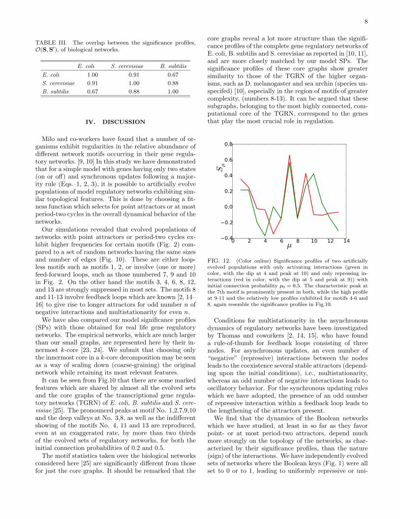
FIG. 9. (Color online) The distributions of number of attractorsof populations with (a) p0 = 0.2 and (b) p0 = 0.5. Bars for theevolved and randomized sets are aligned with the integer values(blue in color) and offset by 0.4 (red in color), respectively. Theblue and red curves are Poisson distributions with the same meanas the evolved and the randomized graphs, respectively. We seethat, the number of different attractors a model graph has, i.e.,multistationarity, is suppressed as the mean degree is increased.

an evolutionary process. In Fig. 7 we compare the in-formation content (the Shannon entropy) of the distribu-tions pF (a) and pr(a) for all the different sets. Definingthe selectivity as the difference between the respectiveinformation contents IF and Ir and normalized by Ir, wehave

s ≡ Ir − IFIr

. (6)

We find 0.46 < s < 0.94 for p0 = 0.2 and 0.38 < s < 0.73for p0 = 0.5, with the mean selectivity being 〈s〉 = 0.65for p0 = 0.2 and 〈s〉 = 0.53 for p0 = 0.5. The smallerselectivity found for p0 = 0.2 is due to the small phasespace of the networks with sparser edges; we have alreadyremarked upon this non-randomizability problem.

From Fig. 8 we see that, for the evolved sets, there isno correlation between the mean attractor lengths and

the mean degrees. On the other hand, for the random-ized sets, there is a clear correlation between the meandegree and the mean attractor length; 〈a〉 increases withincreasing mean degrees 〈k〉, in general. Aldana et al.have found [5] a similar result for Kauffman networkswith random Boolean functions, where a greater densityof edges leads to longer attractors.

The averaged distribution of the number of attractorsNA of the evolved and randomized graphs is given inFig. 9. We observe that for p0 = 0.2, there is a cleardominance of attractors which are transformed to eachother under an exchange of 0 and 1 (equivalently ±1),manifest in the selection of even numbers in the distri-bution. This is because many nodes do not have anyincoming edges, and there are very few with two or moreedges incident on them, so there is no frustration. Thetotal number of attractors are much fewer in the p0 = 0.5networks. The larger initial mean degree leads to a largernumber of instances where an equal number of 1/0 (±1)inputs to the nodes lead to a null argument of the Heav-iside functions in Eqs.(1,3), which breaks the symmetryin favor of 1 as the outcome, allowing us to observe oddnumbers of attractors of a given length.

C. Significance profiles

In Fig. 10 we display our main results for this paper,the significance profiles (SPs) obtained for the 16 inde-pendently evolved populations of 103 model graphs each,for two different initial connection probabilities. Thesetwo sets of profiles have all been obtained at the 400thgeneration of the genetic algorithm, but the profiles showlittle variation once stasis has been achieved. The simi-larity between the significance profiles for the biologicalnetworks and the evolved ones is remarkable, since theonly selection pressure placed on the evolving networkswas the length of their attractors. A more detailed dis-cussion is provided in Section 4.

For a quantitative measure of the similarity betweenthe significance profiles (Eq. 5) of different sets α, β =1, . . .M of evolved or randomized networks, as well asthe overlap of the evolved networks with biological tran-scriptional gene regulatory networks (TGRNs) we havecomputed the following scalar product,

O(S(α),S(β)) =∑µ

S(α)µ S(β)

µ . (7)

The average overlap of a given set α with all the othersets is,

Oα =1

M − 1

∑β 6=α

O(S(α),S(β)) . (8)

The results are reported in Fig.11 for the evolved setsand in Fig. A.2 for their randomized versions. The setshave been sorted with respect to Oα, the sum of all their

7

0 2 4 6 8 10 12 14µ

0.4

0.2

0.0

0.2

0.4

0.6

0.8

1.0Sµ

(a)

0 2 4 6 8 10 12 14µ

0.6

0.4

0.2

0.0

0.2

0.4

0.6

0.8

1.0

Sµ

(b)

FIG. 10. (Color online) Significance profiles S for populationswith initial connection probabilities (a) p0 = 0.2 and (b) p0 = 0.5.The horizontal axis runs over the motif labels, µ, while the verti-cal axis measures the properly normalized, significant deviation ofmotif frequencies from those encountered in the randomized net-works (Eq.5). Thin lines in different colors have been obtainedfor different model populations, while the bold dotted, dashed andcontinuous lines (red, blue and green in color) are the significanceprofiles of the inner k-cores of the gene regulatory networks of E.coli, B. subtilis and S. cerevisiae [25], respectively.

overlaps. In Table III we give the overlaps between bio-logical TGRNs. Numerical results for the mean overlapOα within each set, as well as overlaps of the individ-uals sets with biological networks can be found in theSupplementary Material [22].

In Fig. 11a, one may clearly discern a cluster of fivesets with large mutual overlaps, followed by another clus-ter of three, and in Fig. 11b, an initial cluster of six, fol-lowed by two smaller clusters of 2. It should be noted thatoff-diagonal clusters correspond to groups of sets whichshare a subset of features in their SPs. In Fig. A.2 in theAppendix, where the same matrix is constructed for ran-dom networks, this pattern is lost completely, and halfthe networks have negative overlaps (SP vectors pointingin different directions) indicating more dissimilarity than

FIG. 11. (Color online) The overlap between the significance pro-files of 16 evolved populations with initial connection probability(a) p0 = 0.2 and (b) p0 = 0.5. The overlap matrix has beenarranged to display blocks of networks with the largest overlapsarrayed along the diagonal, by sorting the sets with respect to thelargest total overlap. The numbers correspond to the rank of theset. The color code is given on the side bar. The overlaps are de-fined as the scalar product of the normalized SP vectors (see Eq.7)and take values in the interval [−1, 1].

similarity.

From Table III, we see that the overlap between theTGRNs of different species can be as high as 91 %, oras low as 67 %. Although a greater number of exampleswould be needed to start drawing conclusions, it is re-markable that E. coli is “farthest” from B. subtilis, withS. cerevisiae placed somewhere in between. Both E. coliand B. subtillis are bacteria, while S. cerevisiae (yeast) isa unicellular eukaryote, i.e., on that branch of the phylo-genetic tree which includes plants and animals. It seemsthat this does not make these two species of bacteriamore similar to each other in the significance profiles ofthe inner core of their TGRNs, than they are to yeast.

8

TABLE III. The overlap between the significance profiles,O(S,S′), of biological networks.

E. coli S. cerevisiae B. subtilis

E. coli 1.00 0.91 0.67

S. cerevisiae 0.91 1.00 0.88

B. subtilis 0.67 0.88 1.00

IV. DISCUSSION

Milo and co-workers have found that a number of or-ganisms exhibit regularities in the relative abundance ofdifferent network motifs occurring in their gene regula-tory networks. [9, 10] In this study we have demonstratedthat for a simple model with genes having only two states(on or off) and synchronous updates following a major-ity rule (Eqs. 1, 2, 3), it is possible to artificially evolvepopulations of model regulatory networks exhibiting sim-ilar topological features. This is done by choosing a fit-ness function which selects for point attractors or at mostperiod-two cycles in the overall dynamical behavior of thenetworks.

Our simulations revealed that evolved populations ofnetworks with point attractors or period-two cycles ex-hibit higher frequencies for certain motifs (Fig. 2) com-pared to a set of random networks having the same sizesand number of edges (Fig. 10). These are either loop-less motifs such as motifs 1, 2, or involve (one or more)feed-forward loops, such as those numbered 7, 9 and 10in Fig. 2. On the other hand the motifs 3, 4, 6, 8, 12,and 13 are strongly suppressed in most sets. The motifs 8and 11-13 involve feedback loops which are known [2, 14–16] to give rise to longer attractors for odd number n ofnegative interactions and multistationarity for even n.

We have also compared our model significance profiles(SPs) with those obtained for real life gene regulatorynetworks. The empirical networks, which are much largerthan our small graphs, are represented here by their in-nermost k-core [23, 24]. We submit that choosing onlythe innermost core in a k-core decomposition may be seenas a way of scaling down (coarse-graining) the originalnetwork while retaining its most relevant features.

It can be seen from Fig.10 that there are some markedfeatures which are shared by almost all the evolved setsand the core graphs of the transcriptional gene regula-tory networks (TGRN) of E. coli, B. subtilis and S. cere-visiae [25]. The pronounced peaks at motif No. 1,2,7,9,10and the deep valleys at No. 3,8, as well as the indifferentshowing of the motifs No. 4, 11 and 13 are reproduced,even at an exaggerated rate, by more than two thirdsof the evolved sets of regulatory networks, for both theinitial connection probabilities of 0.2 and 0.5.

The motif statistics taken over the biological networksconsidered here [25] are significantly different from thosefor just the core graphs. It should be remarked that the

core graphs reveal a lot more structure than the signifi-cance profiles of the complete gene regulatory networks ofE. coli, B. subtilis and S. cerevisiae as reported in [10, 11],and are more closely matched by our model SPs. Thesignificance profiles of these core graphs show greatersimilarity to those of the TGRN of the higher organ-isms, such as D. melanogaster and sea urchin (species un-specifed) [10], especially in the region of motifs of greatercomplexity, (numbers 8-13). It can be argued that thesesubgraphs, belonging to the most highly connected, com-putational core of the TGRN, correspond to the genesthat play the most crucial role in regulation.

0 2 4 6 8 10 12 14µ

0.4

0.2

0.0

0.2

0.4

0.6

0.8

Sµ

FIG. 12. (Color online) Significance profiles of two artificiallyevolved populations with only activating interactions (green incolor, with the dip at 4 and peak at 10) and only repressing in-teractions (red in color, with the dip at 5 and peak at 9)) withinitial connection probability p0 = 0.5. The characteristic peak atthe 7th motif is prominently present in both, while the high profileat 9-11 and the relatively low profiles exhibited for motifs 4-6 and8, again resemble the significance profiles in Fig.10.

Conditions for multistationarity in the asynchronousdynamics of regulatory networks have been investigatedby Thomas and coworkers [2, 14, 15], who have founda rule-of-thumb for feedback loops consisting of threenodes. For asynchronous updates, an even number of“negative” (repressive) interactions between the nodesleads to the coexistence several stable attractors (depend-ing upon the initial conditions), i.e., multistationarity,whereas an odd number of negative interactions leads tooscillatory behavior. For the synchronous updating ruleswhich we have adopted, the presence of an odd numberof repressive interaction within a feedback loop leads tothe lengthening of the attractors present.

We find that the dynamics of the Boolean networkswhich we have studied, at least in so far as they favorpoint- or at most period-two attractors, depend muchmore strongly on the topology of the networks, as char-acterized by their significance profiles, than the nature(sign) of the interactions. We have independently evolvedsets of networks where the Boolean keys (Fig. 1) were allset to 0 or to 1, leading to uniformly repressive or uni-

9

formly attractive interactions. In comparison to sets withrandomly generated Boolean keys, the attractor lengthswere indeed shorter from the outset. However, the re-sulting significance profiles shown in Fig. 12 exhibit thesame structures as in Fig.10, in particular for the subsetof motifs {6, 7, 8, 9} . The significance profiles at thesefive motifs can be taken as the topological signature ofnetworks selected for short mean attractor lengths.

Acknowledgments It is a pleasure to acknowledgeseveral useful discussions with Eda Tahir Turan and Nes-lihan Sengor.

Appendix:Significance profiles and their overlaps for

randomized networks

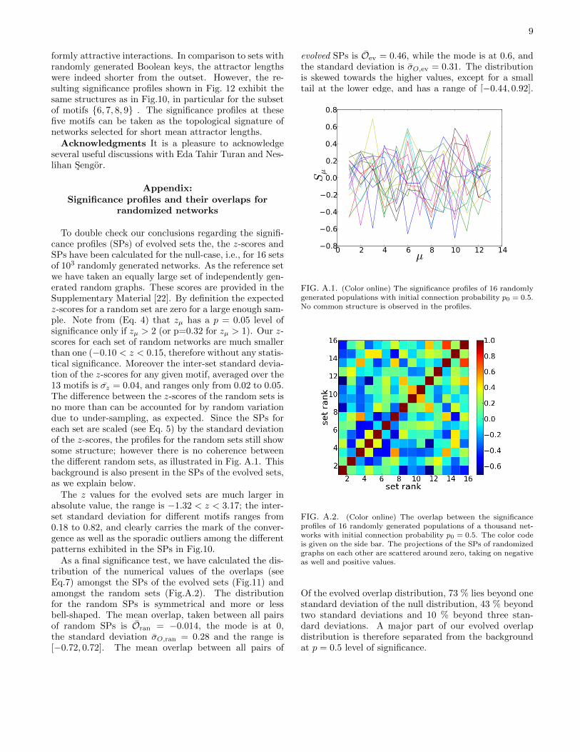
To double check our conclusions regarding the signifi-cance profiles (SPs) of evolved sets the, the z-scores andSPs have been calculated for the null-case, i.e., for 16 setsof 103 randomly generated networks. As the reference setwe have taken an equally large set of independently gen-erated random graphs. These scores are provided in theSupplementary Material [22]. By definition the expectedz-scores for a random set are zero for a large enough sam-ple. Note from (Eq. 4) that zµ has a p = 0.05 level ofsignificance only if zµ > 2 (or p=0.32 for zµ > 1). Our z-scores for each set of random networks are much smallerthan one (−0.10 < z < 0.15, therefore without any statis-tical significance. Moreover the inter-set standard devia-tion of the z-scores for any given motif, averaged over the13 motifs is σz = 0.04, and ranges only from 0.02 to 0.05.The difference between the z-scores of the random sets isno more than can be accounted for by random variationdue to under-sampling, as expected. Since the SPs foreach set are scaled (see Eq. 5) by the standard deviationof the z-scores, the profiles for the random sets still showsome structure; however there is no coherence betweenthe different random sets, as illustrated in Fig. A.1. Thisbackground is also present in the SPs of the evolved sets,as we explain below.

The z values for the evolved sets are much larger inabsolute value, the range is −1.32 < z < 3.17; the inter-set standard deviation for different motifs ranges from0.18 to 0.82, and clearly carries the mark of the conver-gence as well as the sporadic outliers among the differentpatterns exhibited in the SPs in Fig.10.

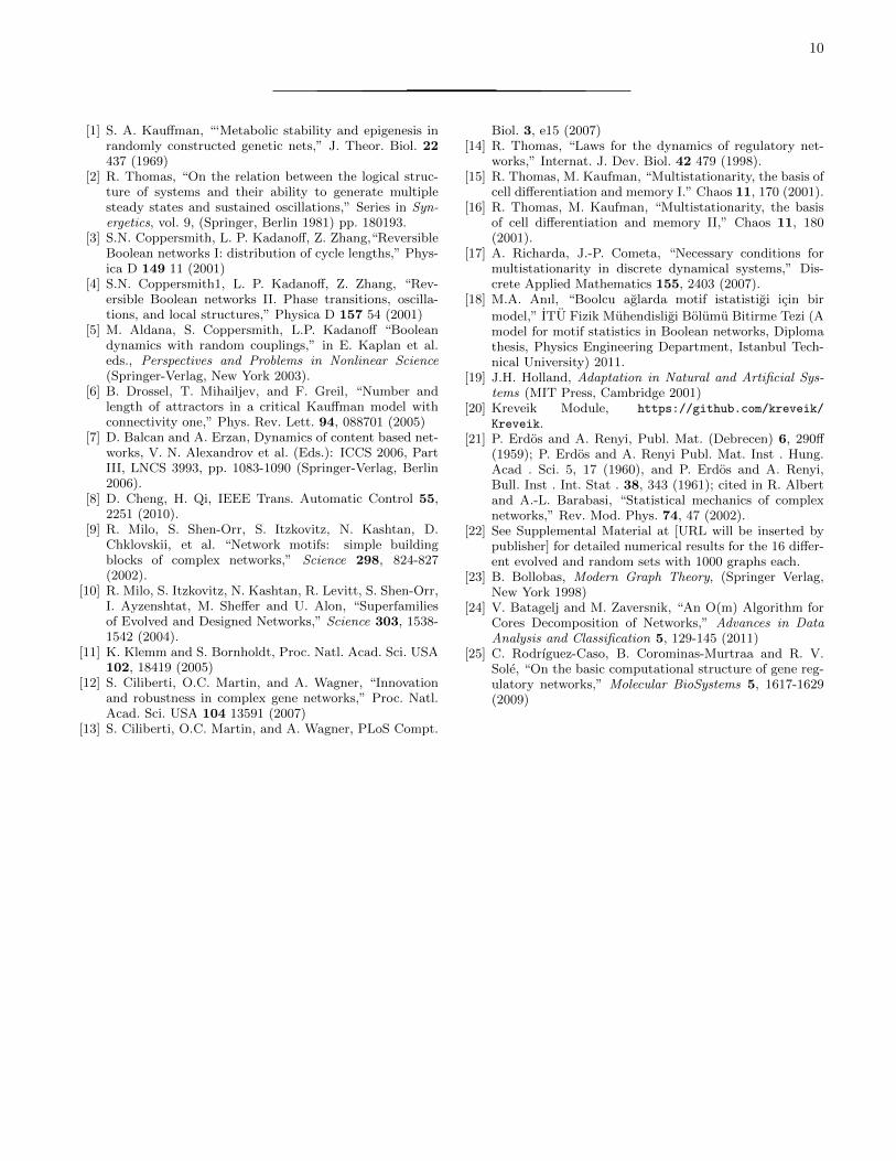
As a final significance test, we have calculated the dis-tribution of the numerical values of the overlaps (seeEq.7) amongst the SPs of the evolved sets (Fig.11) andamongst the random sets (Fig.A.2). The distributionfor the random SPs is symmetrical and more or lessbell-shaped. The mean overlap, taken between all pairsof random SPs is Oran = −0.014, the mode is at 0,the standard deviation σO,ran = 0.28 and the range is[−0.72, 0.72]. The mean overlap between all pairs of

evolved SPs is Oev = 0.46, while the mode is at 0.6, andthe standard deviation is σO,ev = 0.31. The distributionis skewed towards the higher values, except for a smalltail at the lower edge, and has a range of [−0.44, 0.92].

0 2 4 6 8 10 12 14µ

0.8

0.6

0.4

0.2

0.0

0.2

0.4

0.6

0.8

Sµ

FIG. A.1. (Color online) The significance profiles of 16 randomlygenerated populations with initial connection probability p0 = 0.5.No common structure is observed in the profiles.

FIG. A.2. (Color online) The overlap between the significanceprofiles of 16 randomly generated populations of a thousand net-works with initial connection probability p0 = 0.5. The color codeis given on the side bar. The projections of the SPs of randomizedgraphs on each other are scattered around zero, taking on negativeas well and positive values.

Of the evolved overlap distribution, 73 % lies beyond onestandard deviation of the null distribution, 43 % beyondtwo standard deviations and 10 % beyond three stan-dard deviations. A major part of our evolved overlapdistribution is therefore separated from the backgroundat p = 0.5 level of significance.

10

[1] S. A. Kauffman, “‘Metabolic stability and epigenesis inrandomly constructed genetic nets,” J. Theor. Biol. 22437 (1969)

[2] R. Thomas, “On the relation between the logical struc-ture of systems and their ability to generate multiplesteady states and sustained oscillations,” Series in Syn-ergetics, vol. 9, (Springer, Berlin 1981) pp. 180193.

[3] S.N. Coppersmith, L. P. Kadanoff, Z. Zhang,“ReversibleBoolean networks I: distribution of cycle lengths,” Phys-ica D 149 11 (2001)

[4] S.N. Coppersmith1, L. P. Kadanoff, Z. Zhang, “Rev-ersible Boolean networks II. Phase transitions, oscilla-tions, and local structures,” Physica D 157 54 (2001)

[5] M. Aldana, S. Coppersmith, L.P. Kadanoff “Booleandynamics with random couplings,” in E. Kaplan et al.eds., Perspectives and Problems in Nonlinear Science(Springer-Verlag, New York 2003).

[6] B. Drossel, T. Mihailjev, and F. Greil, “Number andlength of attractors in a critical Kauffman model withconnectivity one,” Phys. Rev. Lett. 94, 088701 (2005)

[7] D. Balcan and A. Erzan, Dynamics of content based net-works, V. N. Alexandrov et al. (Eds.): ICCS 2006, PartIII, LNCS 3993, pp. 1083-1090 (Springer-Verlag, Berlin2006).

[8] D. Cheng, H. Qi, IEEE Trans. Automatic Control 55,2251 (2010).

[9] R. Milo, S. Shen-Orr, S. Itzkovitz, N. Kashtan, D.Chklovskii, et al. “Network motifs: simple buildingblocks of complex networks,” Science 298, 824-827(2002).

[10] R. Milo, S. Itzkovitz, N. Kashtan, R. Levitt, S. Shen-Orr,I. Ayzenshtat, M. Sheffer and U. Alon, “Superfamiliesof Evolved and Designed Networks,” Science 303, 1538-1542 (2004).

[11] K. Klemm and S. Bornholdt, Proc. Natl. Acad. Sci. USA102, 18419 (2005)

[12] S. Ciliberti, O.C. Martin, and A. Wagner, “Innovationand robustness in complex gene networks,” Proc. Natl.Acad. Sci. USA 104 13591 (2007)

[13] S. Ciliberti, O.C. Martin, and A. Wagner, PLoS Compt.

Biol. 3, e15 (2007)[14] R. Thomas, “Laws for the dynamics of regulatory net-

works,” Internat. J. Dev. Biol. 42 479 (1998).[15] R. Thomas, M. Kaufman, “Multistationarity, the basis of

cell differentiation and memory I.” Chaos 11, 170 (2001).[16] R. Thomas, M. Kaufman, “Multistationarity, the basis

of cell differentiation and memory II,” Chaos 11, 180(2001).

[17] A. Richarda, J.-P. Cometa, “Necessary conditions formultistationarity in discrete dynamical systems,” Dis-crete Applied Mathematics 155, 2403 (2007).

[18] M.A. Anıl, “Boolcu aglarda motif istatistigi icin bir

model,” ITU Fizik Muhendisligi Bolumu Bitirme Tezi (Amodel for motif statistics in Boolean networks, Diplomathesis, Physics Engineering Department, Istanbul Tech-nical University) 2011.

[19] J.H. Holland, Adaptation in Natural and Artificial Sys-tems (MIT Press, Cambridge 2001)

[20] Kreveik Module, https://github.com/kreveik/

Kreveik.[21] P. Erdos and A. Renyi, Publ. Mat. (Debrecen) 6, 290ff

(1959); P. Erdos and A. Renyi Publ. Mat. Inst . Hung.Acad . Sci. 5, 17 (1960), and P. Erdos and A. Renyi,Bull. Inst . Int. Stat . 38, 343 (1961); cited in R. Albertand A.-L. Barabasi, “Statistical mechanics of complexnetworks,” Rev. Mod. Phys. 74, 47 (2002).

[22] See Supplemental Material at [URL will be inserted bypublisher] for detailed numerical results for the 16 differ-ent evolved and random sets with 1000 graphs each.

[23] B. Bollobas, Modern Graph Theory, (Springer Verlag,New York 1998)

[24] V. Batagelj and M. Zaversnik, “An O(m) Algorithm forCores Decomposition of Networks,” Advances in DataAnalysis and Classification 5, 129-145 (2011)

[25] C. Rodrıguez-Caso, B. Corominas-Murtraa and R. V.Sole, “On the basic computational structure of gene reg-ulatory networks,” Molecular BioSystems 5, 1617-1629(2009)