INFORMATION TO USERS

This manuscn'pt has been reproduced from the microfilm master. UMI films the text directly from the original or copy submitted. Thus, some thesis and

dissertation copies are in typewriter face, while others may be from any type of

computer printer.

The quality of this reproduction is dependent upon the quality of the copy sutxnitted. Broken or indistinct print, colored or poor quality illustrations and photographs, print bleedthrough, substandard margins, and improper

alignment can adversely affect reproduction.

In the unlikely event that the author did not send UMI a complete manuscript and there are missing pages, these will be noted. Also, if unauthorized copyright material had to be removed, a note will indicate the deletion.

Oversize materials (e.g., maps, drawings, charts) are reproduced by

sectioning the original, beginning at the upper left-hand comer and continuing

from left to right in equal sections with small overlaps.

Photographs included in the original manuscript have been reproduced

xerographically in this copy. Higher quality 6” x 9* black and white

photographic prints are available for any photographs or illustrations appearing in this copy for an additional charge. Contact UMI directly to order.

ProQuest Information and teaming 300 North Zeeb Road, Ann Arbor, Ml 48106-1346 USA

800-521-0600

UMI’

EFFECT OF CAVITY PRE-FILL AND GEOMETRY

ON FLOW PATTERNS AND AIR ENTRAPMENT IN THE DIE CAVITY

IN COLD CHAMBER DIE CASTING

DISSERTATION

Presented in Partial Fulfillment of the Requirements for

the Degree Doctor of Philosophy in the Graduate School of

The Ohio State University

By

Bongcheol Park, M.S.

The Ohio State University

2001

Dissertation Committee:

Prof. Jerald R. Brevick^ Adviser

Prof. R. Allen Miller

Prof. Jose Castro

Approved by

Jerald Brevick, Adviser Industrial and Systems Engineering

Graduate Program

UMI Number 3022554

UMI’UMI Microform 3022554

Copyright 2001 by Bell & Howell Information and Learning Company. All rights reserved. This microform edition is protected against

unauthorized copying under Title 17, United States Code.

Bell & Howell Information and Learning Company 300 North Zeeb Road

P.O. Box 1346 Ann Arbor, Ml 48106-1346

Copyright by Bongcheol Park

2001

ABSTRACT

In cold chamber die casting, location, size and total volume of contained

gas porosity are major causes of die casting defects. These attributes of gas

porosity in die casting are influenced by the method chosen to fill the cavity

with molten alloy (or by designing and controlling the metal injection profile).

The alternatives of cavity fill method have provided opportunity to improve

casting quality. Critical slow shot velocity and dual injection method in

squeeze casting are the examples.

Recently, it was observed that controlled acceleration to a critical slow

shot velocity during the slow shot phase could minimize air entrapment in the

shot sleeve. Designing the transition firom slow to fast shot during metal

injection could also potentially minimize air entrapment in the die cavity

during cavity filling. In industry, one common approach in this transition

regime of injection is the cavity pre-fill approach. While the conventional

metal injection approach is to start fast shot immediately after the sleeve and

runner system are full of molten metal with slow shot velocity, the cavity pre­

fill approach has been applied as a different cavity fill approach among someii

die casters. Cavity pre-fill means that the cavity is partially filled with molten

alley using slow shot velocity before fast shot starts. Especially, in thicker-

walled automotive castings, the pre-fill approach has shown equal or superior

quality of castings in terms of porosity.

However, injection parameters for machine set points associated with

cavity pre-HU to obtain maximum quality castings, such as pre-hll percentage

and how the cavity pre-fill influences the quality of castings are not known.

The machine set points have been determined by trial and error method in

industry. In addition, the effects of cavity geometry (including gates and

vents) associated with injection methods on cavity fill pattern and the

consequent quality of castings are not well known.

In this research, using computer modeling, flow patterns in the die cavity

were visualized when cavity pre-fill was employed. The results showed how

cavity pre-fill influences cavity fill pattern in die cavities. In addition, as a

physical simulation, water analog tests were conducted using tinted water,

transparent dies and a high-speed camera. The results of flow patterns

predicted by computer flow modeling were evaluated using the water analog

experiments. Good agreement was obtained. In addition to the qualitative

analysis of cavity flow, a method to measure the amount of air entrapment in

die cavities in the computer flow model was developed. Time when all the

vents are closed (or sealed) is measured under the assumption that vents are

ui

the only way for the air in the die cavity to escape through. And, the time

estimated and known values of gating flow rates give an amount of metal in

the die cavity at the time and also, the amount of air entrapment in the die

cavity. Employing different parameters associated with cavity pre-fill, this

method made a quantitative estimate of the performance in cavity fill

possible.

Using the computer flow model and the method to estimate the amount of

air entrapment, a numerical experiment was conducted to assess the effects of

cavity pre-fill and geometry on the amount of air entrapment. For the

numerical experiment, a low cost response surface method (LCRSM) was

employed. Using computer generated (by EIMSE criterion), low cost (nested

design) experimental design or array, a designed computer experiment was

conducted to evaluate the significant injection and cavity geometry

parameters associated with cavity pre-fill influencing the amount of

entrapped air in die cavities. The injection parameters were: 1) cavity pre-fill

percentage, 2) transition time from slow to fast shot, and 3) cavity pre-fill slow

shot (gate) velocity. The cavity geometry was parameterized: 1) the ratio of

gate thickness and width to maximum casting thickness and width, 2) gate

angle, and 3) complexity of cavity geometry or flow disturbance associated

with vents arid gates. Based on the results of the experiment, the significance

of main effects andT interactions among the above parameters were

IV

investigated. Also, a quadratic polynomial regression model to predict the

amount of air entrapment in the die cavity was developed. As the result,

important cavity pre-hll and geometry parameters were identified and

optimum injection parameters based on given cavity geometry were assessed.

It was observed that cavity pre-fill approach generates lateral expansion

(unilateral expansion in 3 dimension) of initial jet flow in the die cavity. The

lateral expansion was found to be a beneficial effect of cavity pre-fill, which

helps reduce air entrapment in the die cavity. As beneficial effects of cavity

pre-fill were observed, the most significant factor that influences air

entrapment in the die cavity was found to be a factor of cavity geometry

associated with locations of vents and gates and its interactions with injection

parameters for cavity pre-fill. Inappropriate combinations of parameters for

cavity pre-fill caused more amount of air entrapment in the die cavity than

not using cavity pre-fill approach. Hence, both injection and geometry factors

should be considered concurrently when optimum values of injection

parameters for the cavity pre-fill approach are determined to minimize the

amount of air entrapment in the die cavity.

To My Parents and Wife

V I

ACKNOWLEDGMENTS

I express sincere appreciation to my adviser. Dr. Jerald R. Brevick, Professor

in the Department of Industrial, Welding and Systems Engineering, for his

guidance and continuous encouragement throughout the graduate study at the

Ohio State University. This research work would not have been possible without

his mental as well as technical support. Thanks also go to other members of my

research committee. Professors R. Allen Miller, J. Castro, and Theodore T. Allen,

for their valuable suggestions and comments.

Special thanks should go to my friends and colleagues including A. Kitting

in the Department of hidustrial. Welding and Systems Engineering for their good

fellowship and help. I offer my greatest appreciation to my father and mother.

They have provided every possible support throughout my study. Finally, to my

wife, Younjin, I sincerely thank you for your enduring years of my study with

patience, understanding and love.

vu

VTTA

October 22,1962

February, 1987

May, 1990

Sep. 1996-Dec. 2000

Mar. 2001 - Present

Bom-Seoul, South Korea

B.S. Mechanical Engineering,

Seoul National University, Seoul, Korea

M.S. Mechanical Engineering

Boston University, Boston, MA

Graduate Research Associate

The Ohio State University, Columbus, OH

Division Process Development Engineer

SPX Corporation, Contech Division

PUBLICATIONS

1. B. Park and J. Brevick, "Effect of cavity pre-fill and geometry on filling

patterns and air entrapment in cold chamber die casting," North American Die

Casting Association (NADCA) Transactions, pp ., November, 2000.

vui

2. B. Park and J. Brevick, "Computer flow modeling of cavity pre-fill effects in

high pressure die casting," North American Die Casting Association (NADCA)

Transactions, pp. 1-8, November, 1999.

FIELDS OF STUDY

Major Field: Industrial and Systems Engineering

Studies in: Manufacturing Engineering

Die Casting Processes and Tooling

Computer Aided Engineering

Design of Experiments

Minor Field: Mechanical Engineering

Studies in: Computer Aided Design / Computer Aided Manufacturing

Minor Field: Industrial and Systems Engineering

Studies in: Bio-dynamics

IX

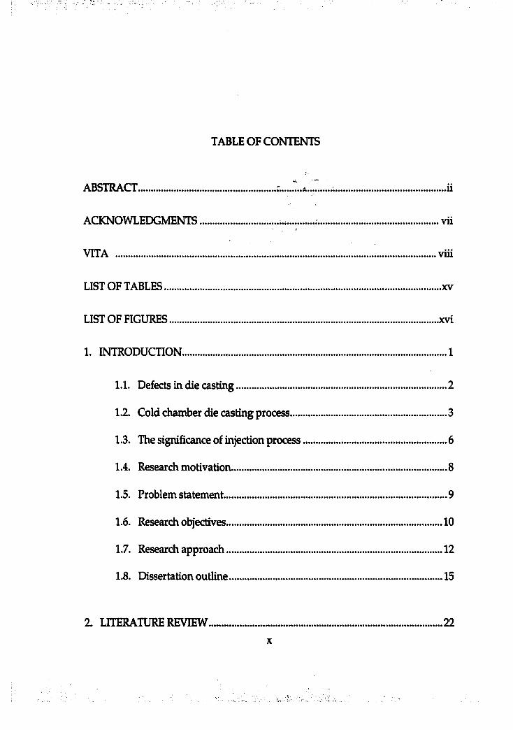
TABLE OF CONTENTS

ABSTRACT...................................................................... ü

ACKNOWLEDGMENTS........................ vü

VITA ................................................................................................................... viii

UST OF TABLES................................................................................................... xv

UST OF FIGURES................................................................................................ xvi

1. INTRODUCTION............................................................................................... 1

1.1. Defects in die casting........................................................................... 2

1.2. Cold chamber die casting process........................................................ 3

1.3. The significance of injection process....................................................6

1.4. Research motivation............................................................................. 8

1.5. Problem statement................................................................................ 9

1.6. Research objectives............................................................................. 10

1.7. Research approach............................................................................. 12

1.8. Dissertation outline.............................................................................15

2. LITERATURE REVIEW....................................................................................22X

2.1. Porosity in die castings......................................................................22

2.1.1. Cause of porosity.....................................................................23

2.1.2. Alternative casting processes to avoid porosity.....................25

2.1.3. Effects of porosity on mechanical properties..........................27

2.2. Die casting machine shot control......................................................28

2.2.1. Process variables and control in die casting............................28

2.2.2. Metal injection system.............................................................31

2.2.3. Machine shot control system.................................................. 32

2.2.4. Shot profile control in cold chamber die casting.................... 33

2.2.5. PQ2 diagram............................................................................ 35

2.3. Fluid flow in the shot sleeve.............................................................. 43

2.4. Fluid flow in die cavities....................................................................47

2.4.1. Filling patterns........................................................................ 47

2.4.2. Optimum fill time....................................................................58

2.4.3. Atomized flow.........................................................................63

2.5. Flow modeling in die casting processes............................................69

2.5.1. Mathematical modeling...........................................................69

2.5.2. Computer modeling of cavity flow........................................ 73

2.5.3. Water modeling........:...................... 81

2.6. Previous work in cavity pre^@f. ........................................87

2.7. Overview................................................. 95

xi

3. COMPUTER FLOW MODELING................................................................ 100

3.1. Two dimensional computer flow model...........................................100

3.1.1 Modeling of cavity pre-fill................................................... 101

3.1.2. Cavity pre-fill vs. conventional cavity fill............................ I l l

3.1.3. Effects of selected parameters.............................................. 113

3.2. Three dimensional computer flow model...................................... 131

3.2.1. Modeling............................................................................... 131

3.2.2. Pre-fill effects on flow pattern.............................................. 134

3.2.3. Gravity effect in cavity pre-fill............................................. 144

3.3. Evaluation of quantitative estimation............................................. 146

3.3.1. Estimation of amount of air entrapment...............................146

3.3.2. Evaluation of estimation ..........................................152

4. WATER MODELING..................... 156

4.1. Die cavity design.............................................................................. 156

4.2.’ Gate and runner design.................................................................... 161

4.3. Transparent die................................................................................ 165

4.4. Experimental setup...........................................................................170

4.5. Dynamic similarity...........................................................................174

4.6. Water model vs. Computer model...................................................175

5. COMPUTER EXPERIMENT......................................................................... 180

xii

5.1. Modeling..........................................................................................180

5.2. Parameters investigated.................................................................. 181

52.1. Injection parameters..............................................................181

5.2.2. Geometry parameters........................................................... 181

5.3. Design of experiment.......................................................................194

5.4. Regression model.............................................................................201

5.5. Conclusions and discussion............................................................ 216

6. EXPERIMENTAL CASTINGS...................... ..:....... 219

6.1. Experiment 1 ...................................................................................219

6.2. Experiment 2 ........................................... 235

7. CONCLUSIONS AND FUTURE WORK....................................................... 244

7.1. Conclusions.....................................................................................244

7.2. Future w ork.....................................................................................247

APPENDIX A: Calculation of Gas Contents in Vacuum Fusion Test................. 249

APPENDIX B: Calculator for Estimation of Trapped Air Volume................. 251

APPENDIX C: Planning for Numerical Experiment....................................... 253

APPENDIX D: Array of Design of Experiment................................................255

APPENDIX E: Calculations for Numerical Experiment..................................257

APPENDIX F: Estimated Responses................................................................. 263

APPENDIX G: Maximum Allowable Cavity Fill Time Calculator................. 265

xiii

APPENDIX H: Estimated Cavity Fill Time....................................................... 267

APPENDIX I: Coefficient of Regression Model and Signiticance of

Factors........................................................................................... 273

APPENDIX J: TT-CP Contour Plot of Regression Model................................ 275

LIST OF REFERENCES........................................................................................ 279

XIV

LIST OF TABLES

Table 2.1. Process variables of cold chamber die casting..................................... 30

Table 2.2. Critical slow shot velocities........................................................ .44

Table 2.3. Physical properties of water and molten alloy.................................85

Table 3.1. Estimated volume of trapped air in the die cavity of Pac Man 151

Table 3.2. Amount of gas contents-Estimate vs. Experiment result...............153

Table 4.1. Rao's ratio for runner design........................................................... 163

Table 5.1. Selected parameters and ranges selected.............................................193

Table 5.2. Performance of three different designs...............................................200

Table 6.1. Estimated w eigh t...............................................................................225

Table 6.2. Cavity pre-fill vs. Maximum pressure............................................240

XV

-( A. .

USTOFHGURES

Figure 1.1. Examples of die casting defects........................................................... 17

Figure 1.2. Schematic diagram of hot chamber die casting system...................... 18

Figure 1.3. Schematic diagram of cold chamber die casting system..................... 19

Figure 1.4. Schematic diagram of ladling in cold chamber die casting system 20

Figure 1.5. Typical shot profile.............................................................................. 21

Figure 2.1. The shot system on the vertical squeeze casting machine.................. 37

Figure 2.2. The SSM casting process...................................................................... 38

Figure 2.3. Effect of Porosity.................................................................................. 39

Figure 2.4. Ultimate Tensile Strength vs. Porosity for T6 Heat Treated A206

Aluminum Alloy Castings................................................................... 40

Figure 2.5. Shot overlays with conventional (left) and real time

control (right)...................................................................................... 41

Figure 2.6. PQ Diagram......................................................................................... 42

Figure 2.7. Possible profiles of wave front in a shot sleeve................................... 46

Figure 2.8. Frommer's concept of metal flow within a die cavity.................... 50

Figure 2.9. Filling patterns using high and low injection speed...................... 51

Figure 2.10. Jet Flow Patterns............................................................................... 52

xvi

Figure 2.11. Cavity fill sequence with a gate velocity of 126 ft/sec and

0.5X0.021 in. gate for a plate die 6X4X0.125 in...............................55

Figure 2.12. Flow sequence after stream impingement on one in. dia. core

for a gate velocity of 60 ft/sec with a 0.5X0.125 in. gate in

plate die 6X4X0.125 in.......................................................................56

Figure 2.13. Partial shots of zinc (a and b) and partial shots of aluminum

(c) showing flow of metal around outside of cavity and large

amounts of air entrapment...............................................................57

Figure 2.14. Photographs of the three types of flow.......................................... 66

Figure 2.15. Fill time for die casting (A1380) as influenced by jet type................ 67

Figure 2.16. Onesorge's chart................................................................................68

Figure 2.17. Water Analog results vs. Flow3D results.......................................80

Figure 2.18. Effect of Injection Velocity.............................................................. 90

Figure 2.19. Partial fill effect before fast shot..................................................... 91

Figure 2.20. Partial shot of zinc illustrating fairly uniform filling...................92

Figure 2.21. Mold flow at the critical speed, 0.5 m /sec..................................... 92

Figure 2.22. Effect of pre-charge height prior to secondary charge

on mold flow.......................................................................................93

Figure 2.23. Entrapped air volume ratio (%) vs. Height of

pre-charge (mm)................................................................................94

Figure 2.24. Injection speed vs. Pre-charge height............................................. 94

xvii

Figure 2.25. The velocity effects on flow by Johnson using computer model...... 98

Figure 2.26. Thickness effect on flow pattern associated with lateral

expansion............................................................................................99

Figure 3.1. Schematic shot profiles of cavity pre-fill........................................... 102

Figure 3.2. An input file of Flow3D for 2D cavity pre-fill...................................105

Figure 3.3. A shot profile created by the input of Figure 3.1 in Flow3D.............106

Figure 3.4. Actual shot profiles of cavity pre-fill approach................................. 107

Figure 3.5. Cavity filling sequence-1..................................................................108

Figure 3.6. Cavity filling sequence-2..................................................................109

Figure 3.7. Cavity filling sequence-3..................................................................110

Figure 3.8. No pre-fill (left) vs. 20% cavity pre-fill (right)...................................112

Figure 3.9. Shot profiles for cavity pre-fill............................................................116

Figure 3.10. Cavity geometry: simple and cavity with ribs inside...................... 117

Figure 3.11. The effects of cavity pre-fill onfiOipg patterns in simple die

cavity using 10ms of transition time and 6.4cm (or 2.5 inches)

of gate width »...;................. 122

Figure 3.12. The effects of cavity pre-fill on filling patterns in the cavity with

ribs using 10ms of transition time and 8.9cm (or 3.5 inches) of

gate width......................................................................................... 123

Figure 3.13. The effects of transition time on filling patterns in simple

die cavity using 40% of cavity pre-fill and 6.4cm (or 2.5") of gate

xviu

width................................................................................................. 124

Figure 3.14. The estimated amount of air trapped in the die cavity A: Simple

cavity with wide gate width, 8.9 cm (or 3.5"), B: Simple cavity

with narrow gate width, 6.4cm (or 2.5")............................................ 125

Figure 3.15. The estimated amount of air trapped in the die cavity A: Cavity

with ribs using wide gate width, 8.9cm (or 3.5"), B: Cavity with

ribs using narrow gate width, 6.4cm (or 2.5")................................... 126

Figure 3.16. The effect of prefill velocity (10ms of fixed transition time),

A: Simple cavity with wide gate width, 8.9cm (or 3.5"),

B: Simple cavity with narrow gate width, 6.4cm (or 2 .5")..............127

Figure 3.17. The effect of prefill velocity (10ms of fixed transition time),

A: Cavity with ribs using wide gate width 8.9cm (or 3.5"),

B: Cavity with ribs using narrow gate width, 6.4cm (or 2.5").........128

Figure 3.18. Twedimensional interpolation (curve smoothing) of figure

3.1 4.....................................................................................................129

Figure 3.19. Twedimensional interpolation (curve smoothing) of figure

3.1 5.....................................................................................................130

Figure 3.20. Cavity geometry................................................................................ 133

Figure 3.21. Sequence of cavity fill patter when using cavity prefill................. 135

Figure 3.22. Sequential flow patterns in the simple rectangular cavi^ with

wide and thin chisel gate................................................................... 137

xix

Figure 3.23. Sequential flow patterns in the simple rectangular cavity with

narrow and thick fan gate.................................................................. 138

Figure 3.24. Sequential flow patterns in the simple rectangular cavity with

wide and thin fan gate.......................................................................139

Figure 3.25. Sequential flow patterns in the ribbed cavity with wide and

thin fan gate....................................................................................... 140

Figure 3.26. Sequential flow patterns in the ribbed cavity with narrow

and thick fan gate.............................................................................. 141

Figure 3.27. Sequential flow patterns in the ribbed cavity with narrow

and thick chisel gate...........................................................................142

Figure 3.28. Sequential flow patterns in the ribbed cavity with wide

and thin chisel gate........................................................................... 143

Figure 3.29. Gravity effects on cavity fill pattern.................................................145

Figure 3.30. Pac-Man casting.............................................................................. 147

Figure 3.31. Computer simulation of Pac-Man casting....................................148

Figure 3.32. Experimental casting geometry (mm) and vacuum fusion

test..................................................................................................... 155

Figure 4.1. Simple complexity geometry casting and d ie ............................... 158

Figure 4.2. Intermediate complexity geometry casting and d ie .....................159

Figure 4.3. High complexity geometry casting and die................................... 160

Figure 4.4. Gate and runner for simple and intermediate complexity

XX

cavities................................................................................................ 164

Figure 4.5. Die assembly for simple complexity cavities.................................166

Figure 4.6. Die assembly for intermediate complexity cavities...................... 167

Figure 4.7. Transparent die setup on the test stand..........................................168

Figure 4.8. Assembly of high complexity geometry die (Adapter Plate)...... 169

Figure 4.9. Experimental setup..................... 171

Figure 4.10. Kodak EKTAPRO 4540- HS Motion Analyzer..............................173

Figure 4.11. Water model vs. Computer model in simple plate die cavity.... 176

Figure 4.12. Water model vs. Computer model in intermediate

complexity geometry die cavity....................................................177

Figure 4.13. Water model vs. Computer model in high complexity

geometry die cavity (Adapter Plate)............................................. 178

Figure 5.1. Total width and thickness of casting................................................. 183

Figure 5.2. Minimum flow distance calculated by CastView..............................188

Figure 5.3. Wide and thin chisel gate (3.65 in x 0.04 in =0.146)...........................190

Figure 5.4. Narrow and thick chisel gate (2 in x 0.073 in =0.146)........................ 190

Figure 5.5. Wide and thin fan gate (3.65 in x 0.04 in =0.146)................................191

Figure 5.6. Narrow and thick fan gate (2 in x 0.073 in =0.146).............................191

Figure 5.7. TT-CP plots for simple (left) and complex geometry (right) with

PV=70% of cssv, GW=52.5%, GA=62.5°............................................. 204

Figure 5.8. PV-CP plots for simple Qeft) and complex geometry (right) with

xxi

TT=45 ms, GW=52.5%, GA=62.5“....................................................... 205

Figure 5.9. PV-TT plots for simple (left) and complex geometry (right) with

CP=20%, GW=52.5%, GA=62.5°......................................................... 206

Figure 5.10. GW-GA plots for simple (left) and complex geometry (right)

with CP=20%, TT=45 ms, PV=70% of cssv...................................... 207

Figure 5.11. GW-TT and GW-CP plot for simple geometry with PV=70% of

cssv, CP=20%, PV=70% of cssv, GA=62.5° and TT= 45ms,

PV=70% of cssv, GA=62.50............................................................... 208

Figure 5.12. GW-TT and GW-CP plot for complex geometry with PV=70%

of cssv, CP=20%, PV=70% of cssv, GA=62.5° and TT= 45ms,

PV=70% of cssv, GA=62.50............................................................... 209

Figure 5.13. Effect of gate angle in simple cavity geometry, GA-CP plot

with TT=45 ms, PV=70% of cssv, GW=52.5%.............................. 212

Figure 5.14. Simple geometry cavity with vents at the bottom area................... 214

Figure 6.1. Schematic casting geometry............................................................220

Figure 6.2. Three different shot profiles for no pre-fill, 30%, and 63%

cavity pre-fill................................................................................... 222

Figure 6.3. Casting weight vs. Composite die temperature............................ 223

Figure 6.4. Estimated weights from Table 6-1...................................................226

Figure 6.5. Images of porosity-1 (X-ray)............................................................227

Figure 6.6. Images of|>orôsifÿ-2 (X-ray)............................................................228

xxii

Figure 6.7. Contour plot of regression model (Equation 5.3) when cavity

pre-fill velocity is same as critical slow shot velocity and

FD=1................................................................................................... 232

Figure 6.8. Shot profiles of seven different percentages of cavity pre-fill 235

Figure 6.9. Images of X ray-3 (Castings produced using 62% of cavity

pre-fill)............................................................................................... 237

Figure 6.10. Images of X ray-4 (Castings produced using negative cavity

pre-fill)............................................................................................... 238

Figure 6.11. Cavity pre-fill vs. Average maximum pressure.............................. 241

Figure 6.12. Microstructures of the burst area of the casting (500x).............. 243

xxm

CHAPTERl

INTRODUCTION

Die casting is a casting technology in which the mold cavity is made of a

metallic material, while other casting technologies, such as sand casting,

investment casting employ nonmetallic molds. Metal mold casting is the

predominant way to manufacture net-shape castings. Specifically, about

90% of all aluminum castings produced are metal mold cast by gravity fed,

low pressure, and high pressure [Apelian, 97].

In high pressure die casting process, the molten metal is injected at high

speed and pressure into a metallic die. As one of near net shape

manufacturing processes, the die casting process is a high volume

production rate process, which produces various nonferrous castings

including aluminum, zinc and magnesium alloys with superior surface

finishes. The die casting process can produce a broad range of castings hrom

small and simple shaped parts to large and complex shaped parts, such as

transmission housings and automotive engine blocks. Due to the high

productivity, net shape and good dimensional tolerance, the highest growth

among various metal mold casting technologies is in die casting.

1.1 Defects in die casting

As die castings are produced by forcing molten alloy under pressure into

metal molds and solidifying it in the die, there exist problems of defects in

use of the process. In general, the defects cause unwanted visual or

functional problems of the castings, such as surface blemish, dimensional

error, reduced mechanical properties (decreased tensile strength or increased

tendency for crack propagation), etc.

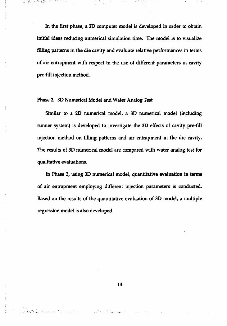
The common defects of die casting are cold laps or cold shuts, flow lines,

lack of fill, solder, witness marks, blisters, cracks, gas porosity, shrinkage

porosity, leaker paths, etc. (Figure 1.1). Cold laps are caused by incomplete

fusion of two different metal streams. Flow lines appear as dark swirls on

the surface. Lack of HU occurs when the melt solidifies in certain regions of

the casting before the die cavity is completely filled. When the cast material

combines with the die steel to form a compound that bonds with the steel

surface, it is called solder. Shiny regions on the casting with a mirror like

appearance are the witness marks. Due to gas bubbles near the surface of

the casting, blisters appear immediately after the casting is ejected or when

the casting is heated. Cracks usually result in the casting due to a cold die.

High die temperature gradients increase the risk of the cracks. Entrapped

air in the melt causes gas porosity. The pores appear as rounded pores with

smooth interior. Shrinkage porosity is generated when the melt solidifies.

Most of the alloys undergo shrinkage on solidification. Shrinkage porosity is

jagged and rough appearance on the interior. Pores formed by shrinkage or

entrained gas can join together forming paths from one to another core or

core to the surface of the casting. These are called leaker paths, which can

cause leakage in the casting [NADCA, 97].

Among those defects, porosity is one of the biggest [NADCA, 97]. Porosity

causes leaks and reduces surface quality and the average mechanical properties

of castings. If pores in castings are eliminated, the tensile strength of aluminum

alloys can be improved significantly [Itamura, 96]. Without porosity, castings are

weldable and heat treatable so that yield strength can be enhanced by heat

treatment [Radtke, 72].

1.2 Cold chamber die casting process

In die casting, it is often introduced that there are two kinds of die

casting systems, which results from trade-offs in metal fluid flow, reactivity

between the molten metal and the metal injection system, and heat loss

during injection. One is 'hot chamber die casting' and another is cold

chamber die casting'.

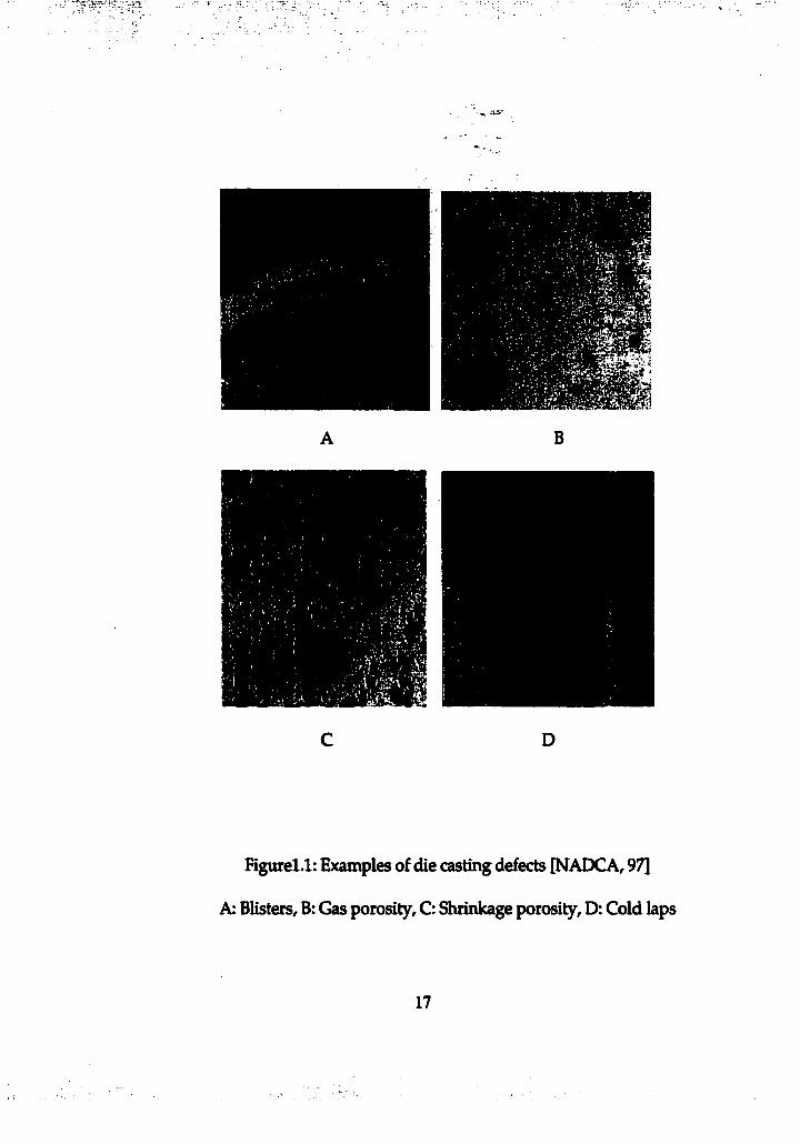
Hot chamber die casting places the hydraulic actuator in intimate contact

with the molten metal (Figure 1.2). The hot chamber process minimizes

exposure of the molten alloy to turbulence, oxidizing air, and heat loss

during the transfer of molten metal. However, prolonged intimate contact

between molten metal and system components presents severe material

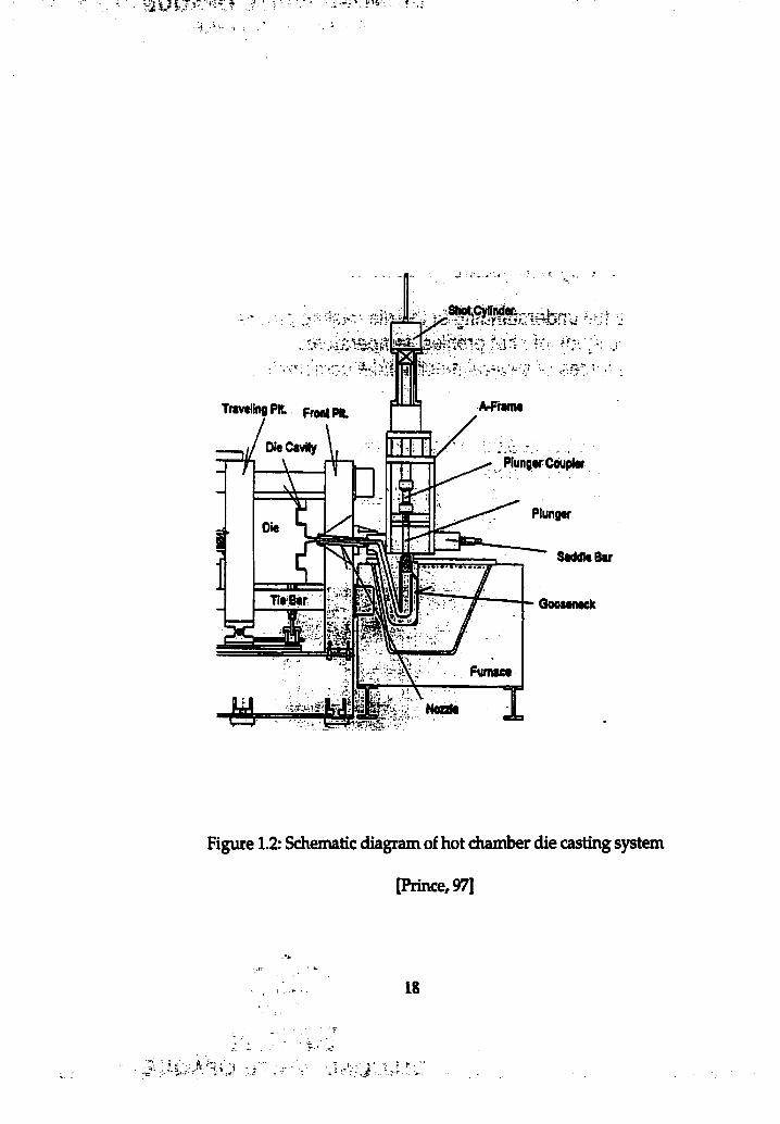
problems. Cold chamber die casting solves the material problems by

separating the molten metal reservoir hrom the actuator for most of the

process cycle (Figure 1.3). The cold chamber die casting requires

independent metering of the metal and immediate injection into the die,

exposing the hydraulic actuator for only a few seconds.

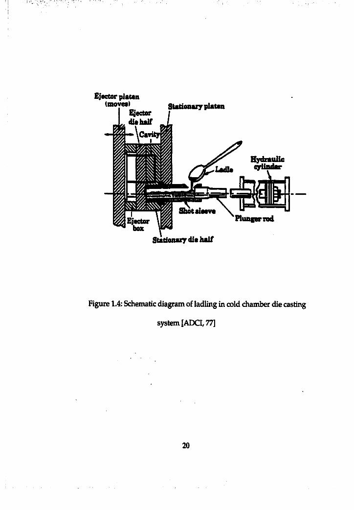
The name, cold chamber die casting', originates hrom the fact that

molten metal is ladled from a furnace into an injection chamber or shot

sleeve which is at relatively low temperature. This ladling process in each

casting cycle is the major difference hom the hot chamber die casting

process (Figure 1.4). After ladling, the plunger is activated to inject molten

metal into a die cavity [Park, 95]. Operating sequence for the cold chamber

die casting process is:T. Die is closed and locked after spraying. 2. Molten

aluminum alloy is t h ^ ladled into the shot sleeve. 3. Plunger moves

forward past the pour hole. 4. Plunger moves forward fast and pushes the

molten into the die cavity. 5. The metal is held under high pressure until it

solidifies. 6. Die opens. 7. Cores retract if present. 8. Ejector pins then eject

the casting kom the ejector die half.

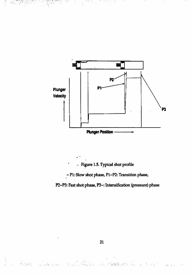
Among the above process steps, the sequence of step 3, 4, and 5 is

injection process of molten alloy into the die cavity, which is normally

achieved in the 4 phases (Figure 1.5). Figure 1.4 represents typical plunger

velocity profile as plunger travels in the cold chamber (i.e. shot sleeve):

1. Slow Shot Phase: In this phase, plunger moves slowly

passing the pour hole so that molten metal does not splash

out through the pour hole. After the plunger moves past the

pour hole, the plunger keeps moving forward until shot

sleeve is filled.

2. Velocity Transition Phase: The velocity of plunger changes

firom slow to desired fast shot velocity.

3. Fast Shot Phase: Once fast shot velocity is achieved, the fast

velocity of the plunger is maintained until the die cavity is

completely filled.

4. Intensification (Pressure) Phase: The plunger stops moving as

the die cavity is filled. After a certain dwell period, high

pressure is applied on the molten alloy while it undergoes

r-'

solidification in the die cavity. The plunger packs metal into

the cavity and feeds shrinkage.

1.3 The significance of injection process in cold chamber die casting

The injection process is one of the most critical phases in die casting process

with respect to the quality of castings produced [Lewis, 87]. Well designed and

controlled injection process plays major role to reduce or control one of the

biggest defects, porosity and porosity related defects. Location, size and

total volume of contained gas porosity are influenced by method chosen to

fill the cavity (i.e. injection process) with molten alloy. For that reason,

reliable shot system for robust metal flow control has been considered to be

crucial in die casting [Thumer, 81].

Gas porosity due to trapped air is an unwanted byproduct of the

relatively high velocity injection method used. Gas entrapment is caused in

the shot sleeve or die cavity by high inertia dominated turbulent jet flow

pattern generated during metal injection process. It would be ideal if high

inertia turbulence during cavity fill could be minimized, so that trapped gas

can be reduced [Walkington, 91]. To reduce inertia of jet flow and

turbulence, and consequently air entrapment in cavity, new techniques of

metal injection have been developed, such as squeeze casting using low

metal injectioii velocity and semi-solid casting using thixotropic HU method.

Vacuum assisted die casting is another example to reduce air entrapment

enhancing air vent. These new techniques have shown considerable promise

in reducing gas porosity, but often increases costs and cycle time.

In die casting, in both industry and university, some efforts have been

made to reduce air entrapment by the modification of injection shot velocity

profile based on the enhanced capability of die casting control systems and

advanced flow study. Slow shot velocity profile in cold chamber die casting,

which is the first phase of common shot profile (Figure 1.5), has been

investigated. Accordingly, optimum (or critical) slow shot profile has been

suggested for industry use to minimize air entrapment in shot sleeve in

horizontal cold chamber die casting [Garber, 82], [Thome, 95]. Regarding

intensification pressure phase, a reclassification of the die-fUling stages is

also suggested by Lui [Lui, 96]. In addition, effects of dual speed injection

for cavity fill were investigated in squeeze casting in order to minimize air

entrapment in cavity [Itamura, 96]. The dual speed injection means that two

different injection speeds (i.e. low speed first and high speed next) are

employed filling die cavities even after shot sleeve is filled. The results of the

research suggested that the conventional third phase (fast shot velocity)

should be broken into two phases for better quality of castings in terms of air

entrapment in die cavities.

1.4Kesearch motivation' I: . . . • ;

Although the most common approach among die casters is to start the

fast shot immediately when the shot sleeve and runner system are just full of

metal, there is a subset of the industry that significantly delays the onset of

the fast shot, sometimes as late as when 30% of the die cavity is already full

of metal. This practice of "cavity pre-filling" dies has been demonstrated to

produce castings having equal or superior quality in terms of porosity and

surface finish when compared to castings made by the conventional

technique. For example, on three different jobs, one commercial die caster

uses no "pre-fill", 45% "pre-fill", and 28% "pre-fill", respectively. However,

each of these injection profiles was determined by trial and error.

Furthermore, when considering any degree of pre-fill, the transition time or

acceleration of the plunger fiom slow to fast injection velocity is suspected

to have a significant influence on the way that the molten alloy flows into

the die cavity.

Squeeze casting uses a very slow velocity to fill the cavity resulting in a

contiguous flow firont (in essence a 100% pre-fill). Pre-filling to a lesser

degree (say 10% to 30%) in conventional die casting may also result in more

contiguous or controlled atomized bront which could aid in minimizing

porosity.

8

1.5 Problem statem ent

The machine shot profile (metal injection parameters) chosen to fill the

cavity with molten alloy has been shown to have a significant influence on

cavity filling patterns and air entrapment. In cold chamber die casting, the

acceptability of castings is often dependent upon the location, size, and total

volume of contained gas porosity formed by the entrapped air.

In recent years, it was reported that even after shot sleeve and runner

system is filled, dual speed injection in cavity fill stage (i.e. low speed prior

to high-speed injection) is effective to avoid air entrapment [Itamura, 95]. In

addition, in industry, some various degrees of cavity pre-fill(up to 45%) have

been applied [Pribyl, 97] and these practices have shown equal or superior

quality of castings in terms of porosity and surface finish. However,

injection parameters for maximum quality casting and how pre-fill effects on

cavity filling are not known since most machine shot profiles are determined

by trial and error method.

There are almost 1m infinite number of ways to approach filling a die

cavity. This is possible due to the development of die casting machine

controls (e.g. control systems provide up to 6 programmable velocity set

points with respect to plunger positions [Dinehart, 98]). The problem is that

the best approach to engineering cavity filling to minimize gas entrapment is

not known.

1.6 Research objectives

The objectives of this research are to:

1) visualize and investigate cavity fill pattern employing cavity pre­

fill injection method vs. conventional cavity fill method to

minimize overall cavity fill time, in which fast shot starts

immediately after shot sleeve is filled,

2) identify important injection parameters associated with cavity

pre-fill and geometry parameters, and analyze quantitatively by

measuring the performance in terms of air entrapment in die

cavities employing different shot parameters,

3) investigate the significance of determined important parameters

influencing air entrapment,

4) assess the best approach to the optimum values of the

determined important parameters.

The injection parameters investigated are: 1) slow shot cavity pre-fill

velocity, 2) pre-fill percentage (or fast shot transition point), and 3) plunger

10

acceleration rate from slow to fast shot In addition, the effects of various

cavity geometries are investigated, such as 1) ratio of gate thickness and

width to maximum casting thickness and width, 2) gate angle, and 3) flow

disturbance.

Based on the investigation of the effect of injection parameters associated

with pre-fill, an optimum machine shot profile in terms of air entrapment in

the die cavity can be obtained considering the capability of up-to-date shot

control systems. The overall objective of this research is to develop a

comprehensive approach to engineering the shot profile (from slow shot to

fast shot phase), so as to minimize air entrapment. This work is a follow-on

to the critical slow shot profile work, which was accomplished earlier for

minimizing trapped air in shot sleeve in cold chamber die casting.

The investigation and establishment of the best approach to optimum (in

terms of air entrapment) injection parameters associated with pre-fill

provides quality castings reducing the machine parameter "tryout" time due

to trial and error method for quality castings. Also, the results of this

investigation of cavity geometry parameter efiects can help engineers select

more effective vent locations during die design phase.

11

1.7 Research approach

Investigation of qualitative effect on flow patterns

Computer flow model using Flow3D is employed to visualize and

investigate cavity fill pattern since more precise parameter controls can be

achieved than available physical simulation method, such as water model

visualizing cavity flow pattern. Using the physical simulation method,

unwanted (and uncontrollable) physical factors are often found, such as

inaccurate and inconsistent plunger speed due to the temperature change of oil

in hydraulic pressure line. The poor controllability of plunger speed makes

heavy parametric study of this research very difficult.

The water analog test is conducted to evaluate the qualitative flow patterns

obtained through the computer flow model. Since there are difliculties to

achieve the wanted values of parameters in water analog test as mentioned

earlier, some selected cases of numerical model are evaluated being compared

with water model.

12

Investigation of quantitative effect on aie entrapment

Using the computer flow model, a semi-quantitative method to measure

performance in terms of amount of total air entrapment in die cavities is

suggested. For the evaluation of cavity geometry effect on air entrapment,

geometry factors are introduced as well. Using response surface

methodology in numerical experiment, a designed experiment is conducted

and the significance of main effects and interactions among factors (or

parameters) are determined. As a result, important metal injection and

cavity geometry parameters are identified. Also, for the selected factors or

parameters, a regression model on the response of air entrapment is

developed and the optimum values of the parameters are determined.

The semi-quantitative model is evaluated by experimental casting results

and the regression model developed using computer experiments is

evaluated by case study.

Phase I: 2D Numerical Model

As previously indicated, Flow3-D® is chosen as a platform to develop a

pre-flUed cavity flow model using excellent mold filling modeling capability

with superior free surface modeling capability which allows the handling

free surface breakup.

13

In the fîrst phase, a 2D computer model is developed in order to obtain

initial ideas reducing numerical simulation time. The model is to visualize

filling patterns in the die cavity and evaluate relative performances in terms

of air entrapment with respect to the use of different parameters in cavity

pre-fill injection method.

Phase 2: 3D Numerical Model and Water Analog Test

Similar to a 2D numerical model, a 3D numerical model (including

runner system) is developed to investigate the 3D effects of cavity pre-fill

injection method on filling patterns and air entrapment in the die cavity.

The results of 3D numerical model are compared with water analog test for

qualitative evaluations.

In Phase 2, using 3D numerical model, quantitative evaluation in terms

of air entrapment employing different injection parameters is conducted.

Based on the results of the quantitative evaluation of 3D model, a multiple

regression model is also developed.

14

Phase 3: Analysis and Evaluation of Computer Flow Model

As a final phase, all the information obtained from the numerical model

and water model are analyzed with respect to the effects of each injection

and cavity geometry parameters on fill patterns and air entrapment. Based

on the analysis of the computer model, the ideas of the best approach to

injection parameters are established.

The computer flow model is evaluated by comparing experimental data

and case study castings.

1.8 Dissertation Outline

Porosity related defects, fluid flow, flow modeling in die casting, and

previous works on this research are summarized and discussed in Chapter 2.

In Chapter 3, two and three-dimensional computer flow modeling and a

method of measuring air entrapment in the die cavity using computer model

are introduced. In Chapter 4, water analog tests and the results are

discussed. Also, the computer flow model is evaluated qualitatively in this

chapter. Parameterization of cavity geometry, computer generated design of

experiment, and regression model are described in Chapter 5. Case studies

of experimental castings are presented in Chapter 6. Finally, conclusions

15

drawn firom this research and issues for future research are discussed in

Chapter 7.

16

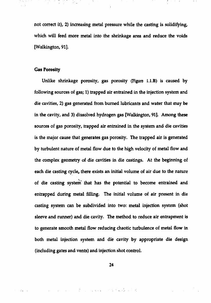
B

Figurel.l: Examples of die casting defects [NADCA, 97]

A: Blisters, B: Gas porosity, C: Shrinkage porosity, D: Cold laps

17

4 , 'r :'. . .-'

-u t W \ m. 'h r j ' ; ;

T f iv t l In g P lL F fo m P K

DkCavUyPlungtrCeupiar

GoOMfMCk

Figure 1.2: Schematic diagram of hot chamber die casting system

prince, 971

18

,r :

ihÉmlIrAeeum.

Mml# F ro n iP M »

w

ShotCyUnd*

ShotConlroiWhw

PMonRod

C d d C h m m b * ' M ungW rR odP k n g w T lp . ;

PtungarRodCoupItr

Figure 1.3: Schematic diagram of cold chamber die casting system

[Prince, 97]

19

Ejector pJaMn(moves) Stationary platen

i

III- II

Hydraulicqrlindmr

Stationary die half

Figure 1.4: Schematic diagram of ladling in cold chamber die casting

system [ADQ, 77]

20

PlungerVelocity

Plunger Position

P3

- Figure 1.5. Typical shot profile

~ PlrSlow shot phase, P1~P2: Transition phase,

P2-P3: Fast shot phase, P3~:Intensification (pressure) phase

21

CHAPTER2

LITERATURE REVIEW

2.1 Porosity in Die Castings

It has been recognized that porosity is one of the most common causes of

defects in die castings. Porosity is considered to be any void within the die

cavity that was not intentionally created. The unwanted porosity influences

the functionality of die castings for certain applications. The negative effects

are as follows: 1) interconnected or through-thickness porosity effects the

pressure tightness or fluid bearing capability, 2) surface porosity, and near

surface porosity exposed by finishing operations, degrades visual aesthetics

of die casting, 3) porosity compromises material properties, and ability of

die casting to function as a load bearing structure, 4) high levels of contained

gas or gas induced porosity limits heat treatment and welding assembly

because of blister formation [Naizer, 92].

22

2.1.1 Causes of Porosity

It is commonly understood that shrinkage and gas are the two major

contributors to porosity [Walkington, 91].

Shrinkage Porosity

Shrinkage induced porosity (Figure l.l.C ) occurs because most cast

metals will occupy less space when they change state from liquid to solid. In

zinc, aluminum and magnesium, the shrink rate will be about 4% to 6% of

the volume [NADCA, 97]. The shrinkage porosity can be subdivided into

two categories. One is macro-shrinkage porosity and another is micro­

shrinkage porosity. The macro-shrinkage porosity is caused by a lack of

directional solidification. Typically, one would like the metal shrinkage

during solidification to be fed by molten metal from the gate. However, in

many cases, due to improper design or a cold die, portions of cavity are cut

off from the source of molten metal. This problem is usually associated with

the hottest local point or the last point to solidify in any given area. Micro­

shrinkage porosity is caused by the limitation of the interdendritic feeding

where the complexities of the dendritic structure make the filling process

more difficult [Verhoeven 75]. The methods of reducing shrinkage porosity

are: 1) changing the temperature balance so as to move the location of the

last point to solidify (whi(^ only moves the location of the porosity and does-•r

23

not correct it), 2) increasing metal pressure while the casting is solidifying,

which will feed more metal into the shrinkage area and reduce the voids

[Walkington, 91].

Gas Porosity

Unlike shrinkage porosity, gas porosity (Figure 1.1.B) is caused by

following sources of gas; 1) trapped air entrained in the injection system and

die cavities, 2) gas generated hrom burned lubricants and water that may be

in the cavity, and 3) dissolved hydrogen gas [Walkington, 91]. Among these

sources of gas porosity, trapped air entrained in the system and die cavities

is the major cause that generates gas porosity. The trapped air is generated

by turbulent nature of metal flow due to the high velocity of metal flow and

the complex geometry of die cavities in die castings. At the beginning of

each die casting cycle, there exists an initial volume of air due to the nature

of die casting systein that has the potential to become entrained and

entrapped during metal filling. The initial volume of air present in die

casting system can be subdivided into two: metal injection system (shot

sleeve and runner) and die cavity. The method to reduce air entrapment is

to generate smooth metal flow reducing chaotic turbulence of metal flow in

both metal injection system and die cavity by appropriate die design

(including gates and vents) and injection shot control.

24

For less turbulent fill method, some various methods, such as squeeze

casting and semisolid metal casting have been developed. Also, in cold

chamber die casting, air entrapment generated in shot sleeve by the

formation and collapse of waves during metal injection was addressed by

Garber and optimal shot velocity profile was investigated at OSU

[Armentrout, 93] [Duran, 91].

2.1.2 Alternative Casting Processes to Avoid Porosity

To avoid or reduce gas and shrinkage porosity caused by traditional

high pressure and high gate velocity die casting process, squeeze casting and

semisolid metal casting have been developed, especially in thick walled

castings.

Squeeze casting, also known as liquid-metal forging, is a hybrid die

casting process which combines features of casting and forging in one

operation and provides wrought-like density and casting configuration

details to give a shaped component having outstanding properties. Squeeze

casting can be divided into two categories; direct squeeze and indirect

squeeze. The direct squeeze casting is close to a forging process, where

castings are made with no gating system. In direct squeeze casting, the raw

material can be in either liquid from or liquid-solid form. On the other

hand, indirect squeeze casting is close to traditional die casting process (both

25

vertical and horizontal cold chamber die systems can be used), but with a

big gate and runner systems. In addition, the shot velocity is much slower

(below 80 in/sec) than that used in conventional die casting process.

According to Yamamoto's (Ube, Japan) mechanical tests, while tensile

strength produced by conventional die casting is 194MPa, that produced by

squeeze casting is 288Mpa. However, although these squeeze technologies

provide significant products benefits, they have not made deep inroads into

die casting technology because of increased costs and longer cycle time

required. The cycle time for squeeze casting ranges from 2 to 3 minutes a

part. This rate is not sufficient to compete with die casting where the less

demanding product quality permits cycle times as short as 20-30 seconds

[Cheng, 95] (Figure 2.1).

The discovery of thixotropic characteristic of semisolid metals at MIT in

the early 1970's provided a new basic approach to producing low porosity or

porosity free castings. Thixotropy is a physical state in which a slurry of

semisolid materials becomes more fluid when a shear force is applied.

Semisolid metal casting and thixoforging have been developed using the

thixotropic characteristic of semisolid metals. In semisolid metal casting, a

specially prepared semisolid metal slug (preheated to the semisolid state) is

used in a die casting machine (semisolid casting) to produce a part

[Jerichow, 95]. This process combines casting and forging (thixoforging) of

26

parts, with cast billet that are forged when 30 to 40 percent liquid

[Kalpalqian, 95]. Using the special physical state of metal, partial liquid

state, the plunger speed is usually below 0.3 m/sec. Sometimes it can even

be lowered to 0.05 m /sec. As a result, the filling flow behavior is laminar, so

that gas entrapment caused by the turbulent nature of traditional die casting

process can be reduced or avoided. Also, shrinkage porosity can be reduced

due to the nature of semisolid material. However, unfortunately, the slow

shot causes defects because of a pre-solidified layer; therefore, the injection

delay time and temperature of the sleeve and die are very important and

must be well selected [Jerichow, 95] (Figure 2.2).

2.1.3 Effects of Porosity on Mechanical Properties

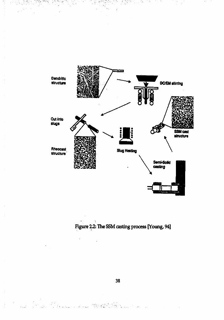
The effect of porosity on the tensile properties of aluminum alloy 601

(6.5 to 7.5 Si, 0.3 to 0.4 Mg, 0.25 Fe, 0.20 Ti,0.05 Cu,0.05 Mn, 0.05 Sr, balance

Al) castings after 16 heat treatment were reported [Eady, 86]. He claimed

that the yield strength, ultimate tensile strength, and hracture elongation, all

decreased with increasing porosity (Figure 2.3). He also stated that even

small levels of porosity are very detrimental as far as ductility is concerned.

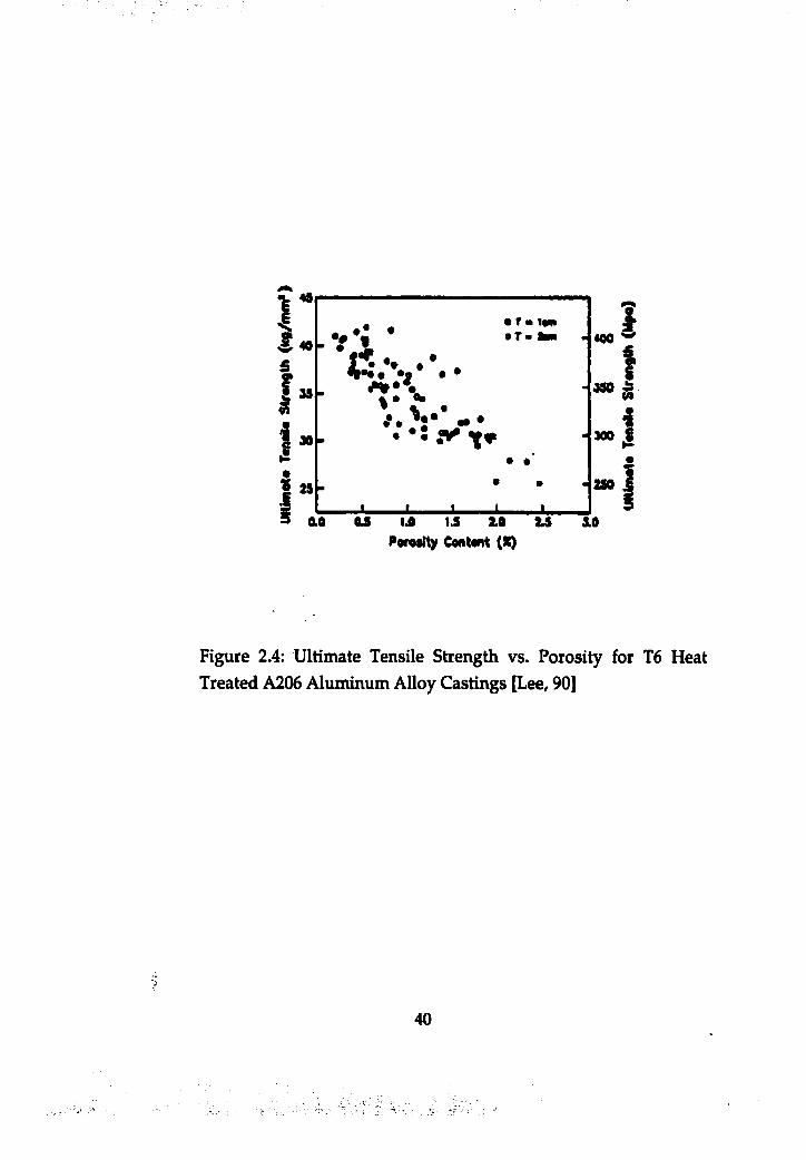
Many researchers, including Lee et al [Lee, 90] and Frabhakar et al

[Prebhakar, 79] have consistently reported that the tensile properties of

materials decrease with increasing levels of porosity (Figure 2.4). Gordon

27

also showed the results of tensile tests that small amount of porosity, in the

range of several volume percent, have detrimental effect on the ultimate

tensile strength and failure elongation of die cast 390 and 380 samples

[Gordon, 93].

22 Die Casting Machine Shot Control

2.2.1 Process Variables and Control in Die Casting

In die casting process, process control is very important for casting

quality due to relatively complex nature of its manufacturing method in

which molten metal is injected at high velocities into reusable metallic molds

and solidified with pressure applied to the casting. The importance of the

control of die casting variables and associated instrumentation has been

emphasized for a long time in industry [Bartling, 66]. It is addressed that

there are eight basic variables that must be controlled in the die castings by

Herman [Herman, 88]: 1) alloy content, 2) holding furnace temperature, 3)

injection velocity, 4) tie bar loading, 5) die temperature, 6) release material,

7) casting ejection temperature, 8) cycle timing. Also, casting variables for

cold chamber die castog is well summarized for instrumentation by Brevick

and Mobley [Mobley, 96[. Table.2.1 shows casting variables in cold chamber

2 8

die casting. Among those casting variables in cold chamber die casting, the

metal injection system variables are among the most critical variables for die

casting since those variables are responsible for controlling all of the flow,

pressure, and trapped substance defects.

29

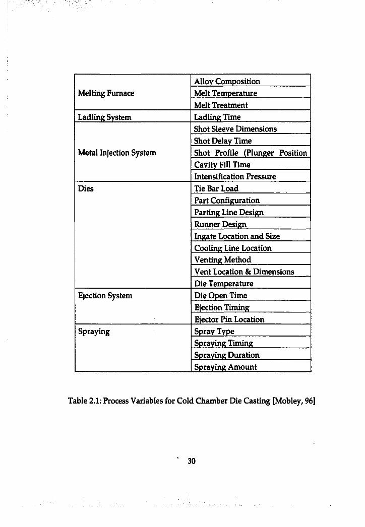
Melting FurnaceAlloy CompositionMelt TemperatureMelt Treatment

Ladling System Ladling Time

Metal Injection System

Shot Sleeve DimensionsShot Delay TimeShot Profile (Plunger PositionCavity Fill TimeIntensification Pressure

Dies Tie Bar LoadPart ConfigurationParting Line DesignRunner DesignIngate Location and SizeCooling Line LocationVenting MethodVent Location & DimensionsDie Temperature

Ejection System Die Open TimeEjection TimingEjector Pin Location

Spraying Spray TypeSpraying TimingSpraying DurationSpraying Amount

Table 2.1; Process Variables for Cold Chamber Die Casting [Mobley, 96]

30

2.2.2 Metal injection system

The abilities to inject the molten metal at extremely fast rates (from 10 to

hundreds milliseconds) and to apply high pressures (up to 40,000 psi) to the

solidifying metal are the features that distinguish die casting from other

casting processes. The principle components of the metal injection systems

are [Herman, 88]:

1) Shot sleeve- cylinder or cold chamber

2) Plunger- water cooled piston in shot sleeve

3) Plunger rod that extends from the plunger to the hydraulic cylinder

4) Coupling that connects the plunger rod to the hydraulic cylinder rod

5) Hydraulic cylinder that converts flow and /o r pressure of the hydraulic

fluid into motion or force on the plunger

6) Control valves to control the direction and speed of the plunger

7) Hydraulic line to carry the pressurized hydraulic fluid

8) Accumulator to store energy in the form of a compressed gas

9) Pump, motor, reservoir, and regulating valves to provide the source of

pressurized fluid necessary to the hydraulic system

10) Intensifier to increase hydraulic pressure in the cylinder after the cavity

31

pressurized fluid necessary to the hydraulic system

Z2.3 Machine shot control system

Since shot end performance and repeatability was recognized to be

important for die casting quality, dynamic real time shot control system has

been introduced by Vann [Vann, 88]. Unlike conventional shot end system

for sequential controls, the system is a closed loop control system using

sensors for feedback, such as Linear Variable Distance Transducer (LVDT)

and piston rod encoder. The LVDT is attached to the spool of a velocity

control valve, and output firom the LVDT provides feedback to the control

system for accurate positioning of the valve spool. The piston rod encoder is

designed to monitor the position and velocity of the machine shot cylinder

and provides critical feedback loop. The feedback signal flom the piston rod

encoder is continuously compared to the input signal from the controller. A

plus or minus following error signal is then output to the servo amplifier

card, which drives actuator, (servo valve) proportional to the signal.

While standard shot hydraulic circuits tend to repeat fairly consistently,

slight changes in plunger tip drag, load pressure, and hydraulic fluid

viscosity can result in variation in the shot profile and the quality achieved.

Using dynamic real time control systems, repeatability of system is

improved compare to conventional systems without real time feedback

32

functions (Figure 2.5). In addition, smooth metal flow can be achieved with

this real time feed back system. Especially, in shot velocity transition phase

(from slow to fast shot), real time acceleration control generates smooth

transition shot profile and as a result, improved surface hnish is observed

[Vann, 93].

In addition to the above advanced shot control system capabilities,

recent die casting machines used in industry have up to 10 ms of maximum

transition time from slow to fast [Walkington, 98]. For the flexibility of shot

profile programming, injection control system panel provides up to six

velocity-set-points with respect to plunger position even though only 3 or 4

set points are usually utilized in industry (e.g. VisiTrak control system)

[Dinehart, 98].

2.2.4 Shot Profile Control in Cold Chamber Die Casting

As stated earlier, typically, injection process of molten alloy is divided

into four phases as plunger travels in the shot sleeve: slow shot phase,

velocity transition phase, fast shot phase, and intensification phase.

The main purpose, of the control of slow shot phase is to carry molten

alloy in the shot sleeve to the gates of the cavity with minimum air

entrapment in the shot sleeve. If plunger moves relatively high speed in the

shot sleeve, wave front will curl over and entrap air. On the other hand, if

33

plunger moves relatively low speed in the shot sleeve, the reflected wave

will cause air entrapment. Therefore, investigators have noticed the

existence of a critical slow shot velocity, which minimize the amount of air

entrapment in the shot sleeve. Critical velocity is defined as the velocity

required to raise the wave formed in front of the plunger tip to the top of the

shot sleeve chamber without its rolling [Armentrout, 93].

Once shot sleeve and runners are filled with molten metal using the

optimum slow shot velocity, fast shot is engaged. The fast shot is to fill the

cavities before molten alloy solidifies. In high-pressure die casting

processes, fast shot is especially important. The fast cavity fill makes it

possible to produce thin walled complex geometry castings, where

solidification time is relatively short. Unfortunately, the fast shot usually

generates air entrapment associated with high turbulence of metal flow in

die cavities. For that reason, fast shot should be properly controlled along

with the velocity transition from slow to the fast shot [Walkington, 98].

As soon as the cavity is filled, intensification pressure is engaged in the

die cavity. This intensification pressure squeezes metal in the die cavity

while the molten metal solidifies. This procedure helps produce complex

geometry castings and is one of the important features of die casting

processes. Although high intensification generally reduces shrinkage

34

porosities in castings, too much pressure generates unwanted results, such

as metal flash [Walkington, 91].

2.2.5 PQ^ diagram

Based on Bernoulli's energy balance equation accounting for energy

losses due to hiction, pressure-flow rate square (PQ^) diagram has been

developed to help evaluate die casting machine's capabilities and the

pressure required to fill the die cavity. This diagram provides a means of

determining the actual filling time and gate velocity of the liquid metal.

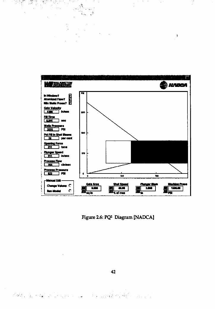
PQ2 diagram was made by plotting the maximum achievable velocity of

the plunger (dry shot) along the horizontal axis and maximum hydraulic

pressure along the vertical axis (Figure 2.6). An angled line connecting these

two points defines the 'pressure available line'. This line shows that

machine's pressure capability is not constant and depends on metal flow rate

and shot speed. In addition, on the same diagram, 'pressure required line'

for planned plunger velocity is created based on the calculation of Darcy's

equation with’discharge coefficient, which represents energy loss.

Based on these two lines, some modification of operation parameters or

operation plan can be made for the casting quality, such as gate velocity,

accumulator pressure, and plunger diameter [Herman, 88], [Zabel, 80].

35

Recently, regarding discharge coefficient in Darcy's equation, Bar-Meir

claims that the discharge coefficient is not constant and it is a function of the

runner geometry, which relates to the cross section size, length and metal

feed system configuration [Bar-Meir, 97].

36

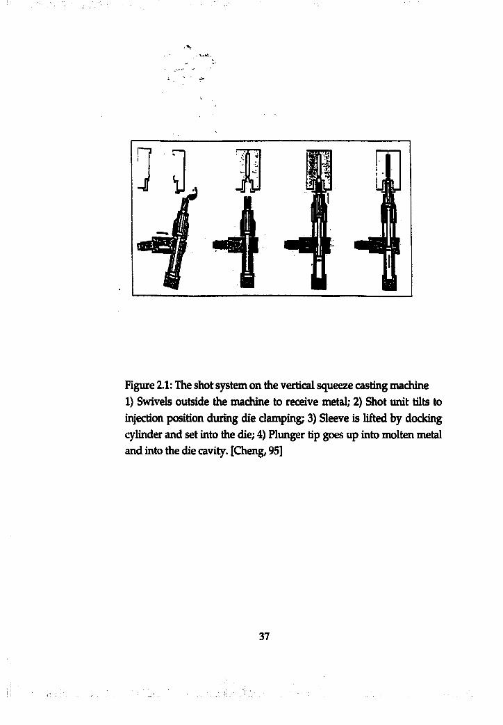
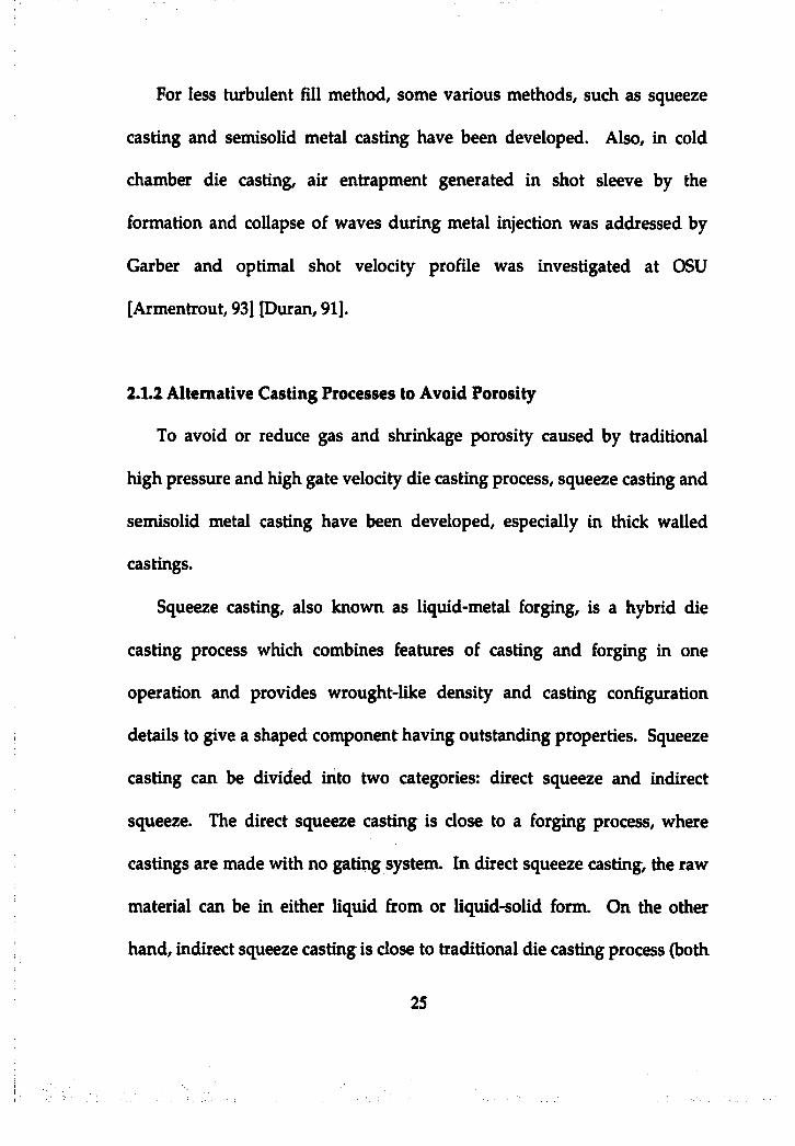
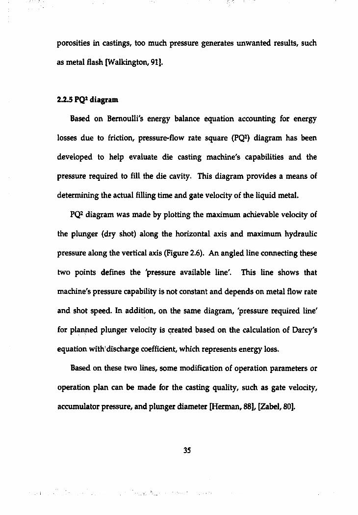
Figure 2.1: The shot system on the vertical squeeze casting machine 1) Swivels outside the machine to receive metal; 2) Shot unit tilts to injection position during die damping; 3) Sleeve is lifted by docking cylinder and set into the die; 4) Plunger tip goes up into molten metal and into the die cavity. [Chengs 95]

37

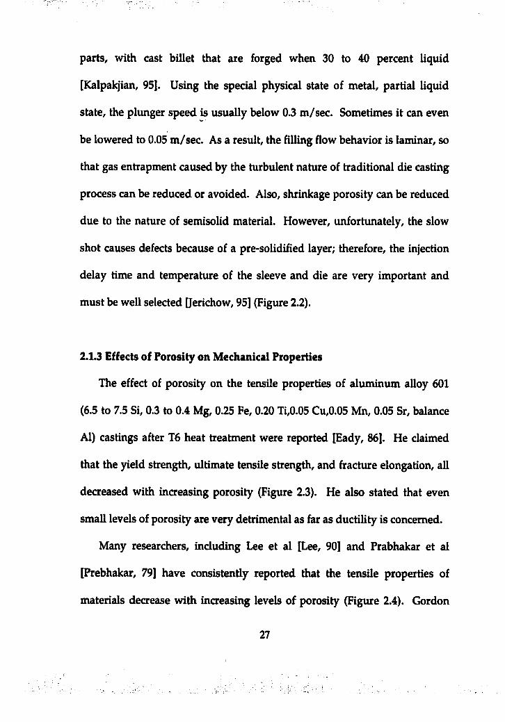
OendrWcstructure

Cut into slugs

Rheocaststructure

DC/EM stirring

Slug Hating

Figure 2.2: The SSM casting process [Young, 94]

38

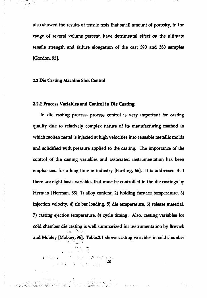
OkStO'Ili» t Mt

• 1 2 1 l S I 7Ponsity (%)

rm.MTwl» M# OAStn-17)» Mn< Ml

» a J 5 i 7Ftrosity (%)

Figure 2.3: Effect of Porosity [Eady, 86]

Left) Ultimate Tensile Strength of 601 Al alloy; Right) Tensile Elongation of 601 Al alloy

39

MO A

. 250

a s 1.0 1.S 10 i sPwWty Contant (%)

Figure 2.4: Ultimate Tensile Strength vs. Porosity for 16 Heat Treated A206 Aluminum Alloy Castings [Lee, 90]

40

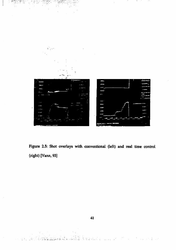
Figure 2.5: Shot overlays with conventional (left) and real time control

(right) [Vann, 93]

41

«m

biWMowr h MomintfFtowr R MnSMfcPreM? B CgeïW odlyu m I h A , "FMTIim

9jMePrM«ura I I M lfctHilnShimiiwiiI M I P W M B tOgeningtoree I M lPfcmgwSgeedI 1 1 1 I I n M w

_ZM_ cfeiAac P rocw P rew wL « I M l

MmutlEdi-------ClMngBValiiM C

C

p»

sn

TM

i r a 1SIwISp—d

a çPlunowOiiro

m «

Figure 2.6: PQ2 Diagram [NADCA]

42

2.3 Fluid Flow in the Shot Sleeve

Typically, the shot sleeve (cold chamber) is not filled in full due to the

nature of cold chamber die casting system; molten alloy is ladled into pour

hole on the top of shot sleeve (Figure 2.7). Accordingly, the remaining

volume in the shot sleeve is occupied by air.

As molten metal is carried to the cavity gate, the general nature of fluid

movement during slow shot travel in shot sleeve is a wave formation and air

entrapment associated with it. If the slow shot velocity is relatively high, the

wave front will roll over and cause entrapped air. If the slow shot velocity is

relatively low, the reflected wave will trap air in front of the plunger (Figure 2.7).

To avoid this unwanted air entrapment in the shot sleeve. Dr. Lester Garber

investigated flow movement and optimum shot velocity in the shot sleeve. His

theoretical analysis is based on energy considerations, Bernoulli's equation

[Garber, 82]. He claimed that 1) plunger velocity, initial-fill level, and cold

chamber diameter determine air entrapment in the cold chamber, 2) it is possible

to obtain good cold chamber filling conditions at a constant plunger velocity, 3) a

critical slow-shot velocity exists at which air entrapment is minimized.

Many investigators have noticed the existence of a critical slow shot velocity

that will minimize the air entrapment in the shot sleeve. Kami developed a

model to predict wave height as a function of plunger velocity, initial fill

percentages and cold chamber diameter using turbulent bores and hydraulic

43

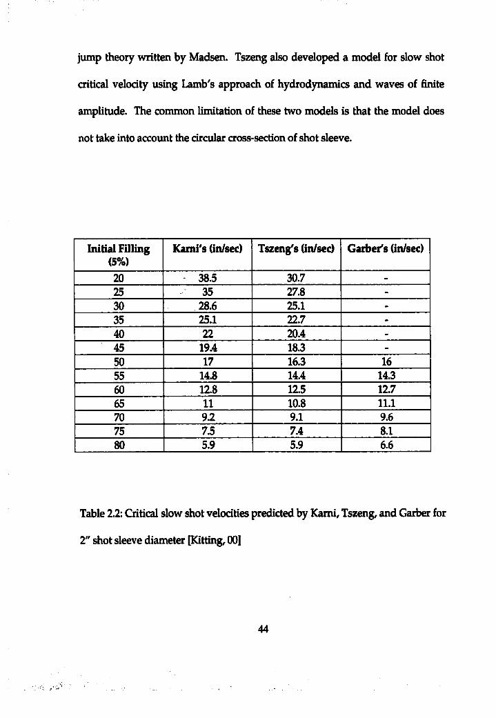
jump theory written by Madsen. Tszeng also developed a model for slow shot

critical velocity using Lamb's approach of hydrodynamics and waves of finite

amplitude. The common limitation of these two models is that the model does

not take into account the circular cross-section of shot sleeve.

Initial Filling (5%)

Kami's (in/sec) Tszeng's (in/sec) Garber's (in/sec)

20 38.5 30.7 -

25 35 27.8 -

30 28.6 25.1 -

35 25.1 22.7 -

40 22 20.4 -

45 19.4 18.3 -

50 17 16.3 1655 14.8 14.4 14.360 12.8 12.5 12.765 11 10.8 11.170 9.2 9.1 9.675 7.5 7.4 8.180 5.9 5.9 6.6

Table 2.2: Critical slow shot velocities predicted by Kami, Tszeng, and Garber for

2" shot sleeve diameter [Kitting, 00]

44

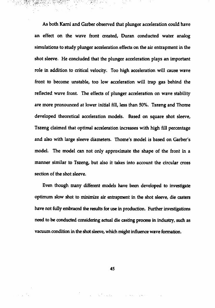
As both Kami and Garber observed that plunger acceleration could have

an effect on the wave front created, Duran conducted water analog

simulations to study plunger acceleration effects on the air entrapment in the

shot sleeve. He concluded that the plunger acceleration plays an important

role in addition to critical velocity. Too high acceleration will cause wave

hont to become unstable, too low acceleration will trap gas behind the

reflected wave hont. The effects of plunger acceleration on wave stability

are more pronounced at lower initial fill, less than 50%. Tszeng and Thome

developed theoretical acceleration models. Based on square shot sleeve,

Tszeng claimed that optimal acceleration increases with high fill percentage

and also with large sleeve diameters. Thome's model is based on Garber's

model. The model can not only approximate the shape of the front in a

manner similar to Tszeng, but also it takes into account the circular cross

section of the shot sleeve.

Even though many different models have been developed to investigate

optimum slow shot to minimize air entrapment in the shot sleeve, die casters

have not fully embraced the results for use in production. Further investigations

need to be conducted considering actual die casting process in industry, such as

vacuum condition in the shot sleeve, which might influence wave formation.

45

m

E

E

1- n ' ‘ Î,

a

*

Figure 2.7: Possible profiles of wave front in a shot sleeve. (1) Preferred (stable) wave front; (2) Wave front roll-over and break­up; (3), (4) Air trapped between the incoming wave front and wave reflected from the far end of the shot sleeve [Tszeng, 92]

46

2.4 Fluid Flow in Die Cavities

Since in die casting, molten metal is injected into complex geometry

cavity with high velocity under high pressure, fluid flow analysis is one of

the most important factors that die casting engineer must consider when

designing process, die with gating system. Both production rate and casting

quality are highly dependent upon the characteristics of fluid flow, which is

influenced by a number of variables, such as injection parameters, alloy

contents, runner/gate system, and casting geometry.

2.4.1 Filling Patterns

The fluid flow in die cavity is a inertia dominated, transient and often

turbulent with Reynolds number in the range of 3000 - 50000 [Frayce, 91]

due to the flow of high velocity molten metal and rapidly changing flow

direction in complex geometry of runner/gate and cavity. The flow of air in

die cavity associated with molten metal flow is also very important flow

problem since the air is supposed to escape through vents during cavity fill

of molten alloy. However, in general, the turbulent nature of molten alloy

coupled with wave formation during the filling, prevents air escape out of

cavity and results in air entrapment that causes unwanted compressed gas

porosity in castings.

47

The nature of molten metal flow in die castings was postulated by

Frommer in 1932 that molten, metal jet flowed from the ingate across the die

cavity, struck the opposite wall, and then, following the inertial forces,

flowed back toward the ingate. It was stressed that the die cavity is filled

progressively back toward the ingate from the opposite wall [Maier, 75]

(Figure 2.8).

Bennet studied flow pattern with different gating approaches using

transparent plastic molds and water as flowing medium. Based on the

images obtained, it is shown how the filling progresses with the stream

collision at the far end, followed by back filling with forerunners along the

side walls preceding the main flooding action, which is same results that

Frommer & Bradt stated earlier [Bennet, 61].

Using interchangeable gate rings, the filling patterns associated with

various different geometry of gates (fan, tangential, and pincer) and injection

parameters (gate velocity and final pressure) was investigated conducting

partial castings and water analog test [Moorman, 62]. Through this test, four

different filling types were well described and addressed; 1) progress fill, 2)

back fill, 3) whirlpool fill, and 4) turbulent fill (Figure 2.9). The results of

this experiment show that gate types and gate velocities are important

parameters in terms of air entrapment during filling.

48

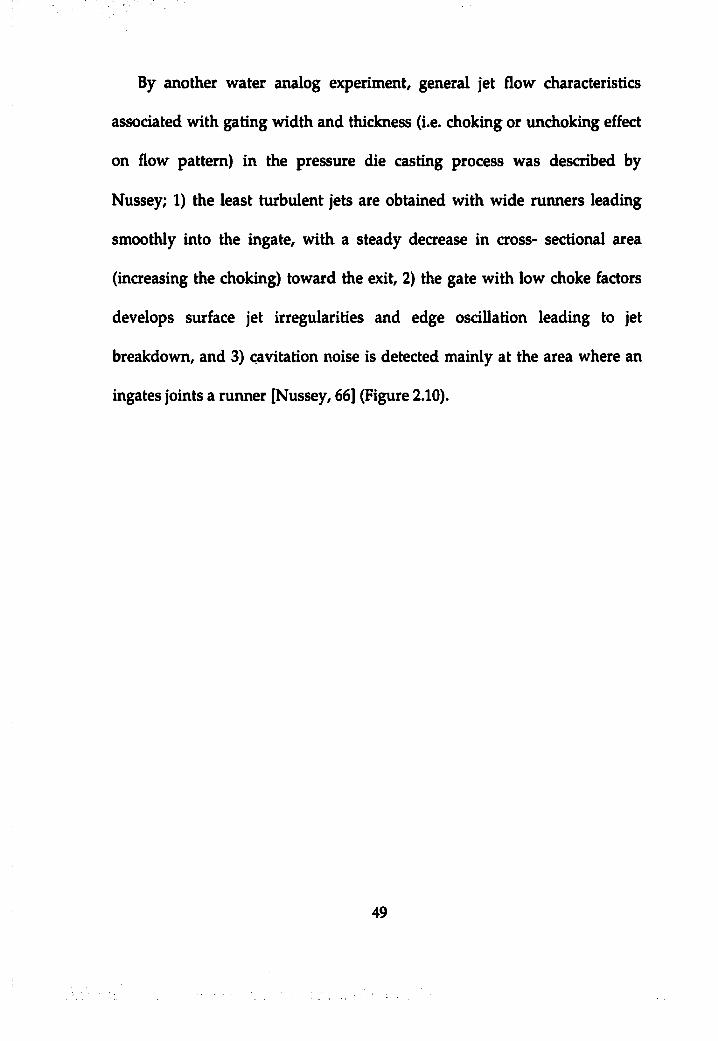
By another water analog experiment, general jet flow characteristics

associated with gating width and thickness (i.e. choking or unchoking effect

on flow pattern) in the pressure die casting process was described by

Nussey; 1) the least turbulent jets are obtained with wide runners leading

smoothly into the ingate, with a steady decrease in cross- sectional area

(increasing the choking) toward the exit, 2) the gate with low choke factors

develops surface jet irregularities and edge oscillation leading to jet

breakdown, and 3) cavitation noise is detected mainly at the area where an

ingates joints a runner [Nussey, 66] (Figure 2.10).

49

%

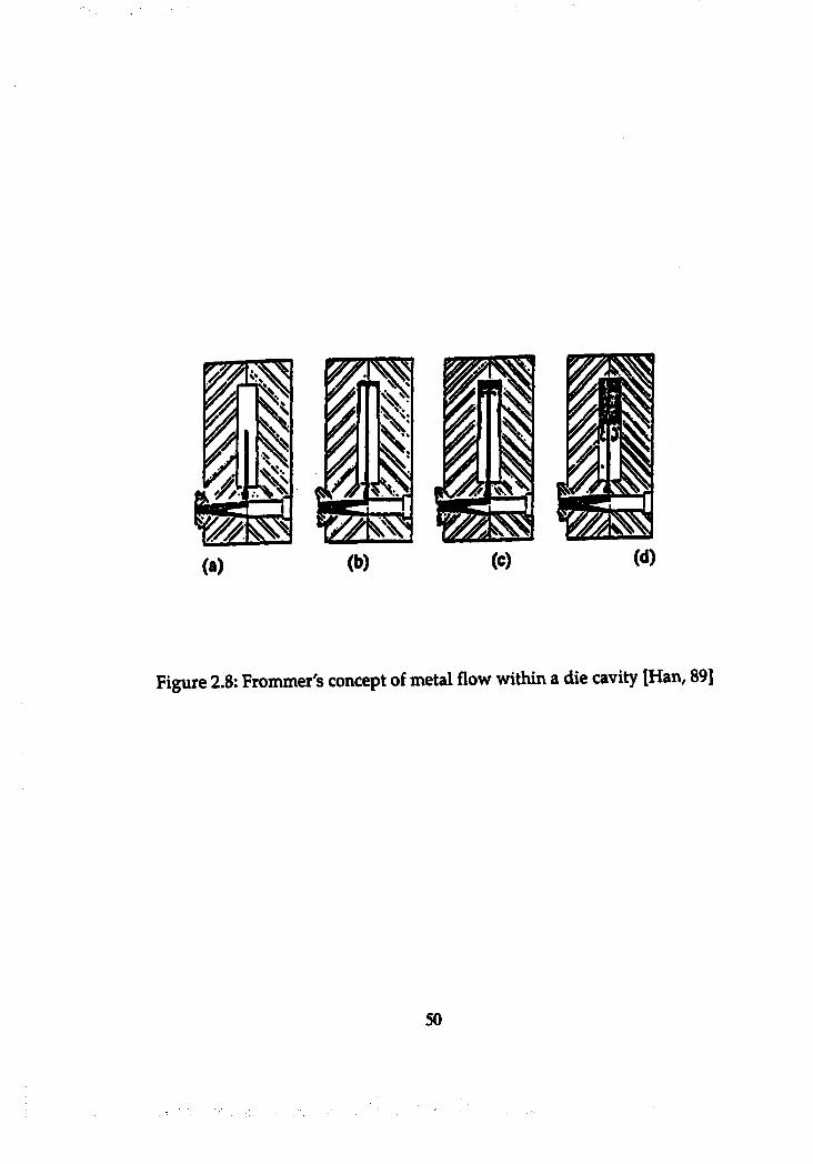
Figure 2.8: Frommer's concept of metal flow within a die cavity [Han, 89]

50

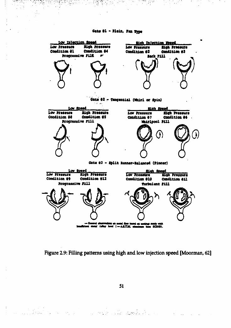
O ê ta # 1 - H a l a , m T y p t

LOW Inlietlon Sp—dXiow vrumra Ceaditlen #1

Blfh ffrtMurt Ceaditlen #4

frefraielve rilC »*

■ieh mitetlcn iewd_&ew rraeeure Ceaditlea #2

ligh vreMuee ceaditlea «I

ladt riU

Oate *2 - Tmngeatiml (Mhirl or Spia)

Lew SewdLOW vroarare High BreeeuraCeaditlea *6 Ceaditlea *S

rregxuiive FUI

JttSjLlew rrtMHze Bigh Froeaureceaditlea #7 ceaditlea #6

WUrlpool FUI

G ) 0

data #3 - Split liiBaar-lalaaead (Flaear)Low Soaad

Low praaaura High FraaawraCORditioa *9 Condition #12

Frograaalva FUI

Hioh soaadlow P r a a a u r a u g n praaaura Condition #10 Ceaditlen #U

Turbwlant FUI

- X

wwa w wn M M i (W br M i - . 4 a . T J i .

â

Figure 2.9: Filling patterns using high and low injection speed [Moorman^ 62]

51

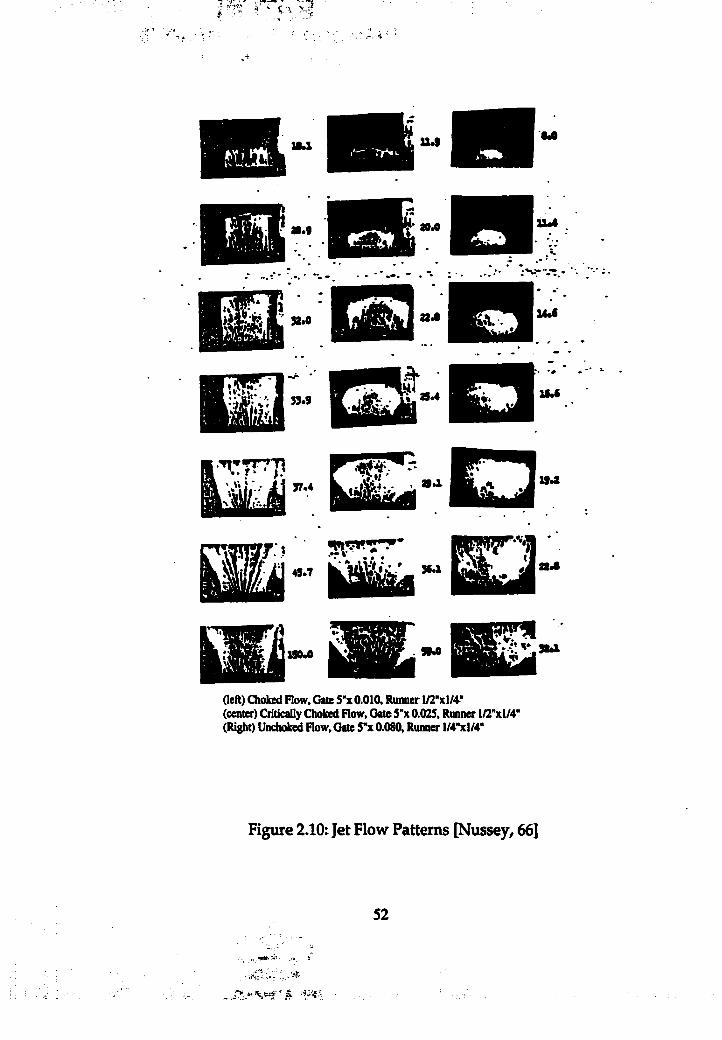
1 9 0 .0 9 9 .0 V r.v 3ta

(left) Choked Flow, Ckte 5"x 0.010, Runner l/2"xl/4"(center) Critically Choked Flow, Gate S”x 0.025, Runner l/2*xI/4” (Right) Unchoked Flow, Gate S”x 0.080, Runner l/4"xl/4"

Figure 2.10: Jet Flow Patterns [Nussey, 66]

52

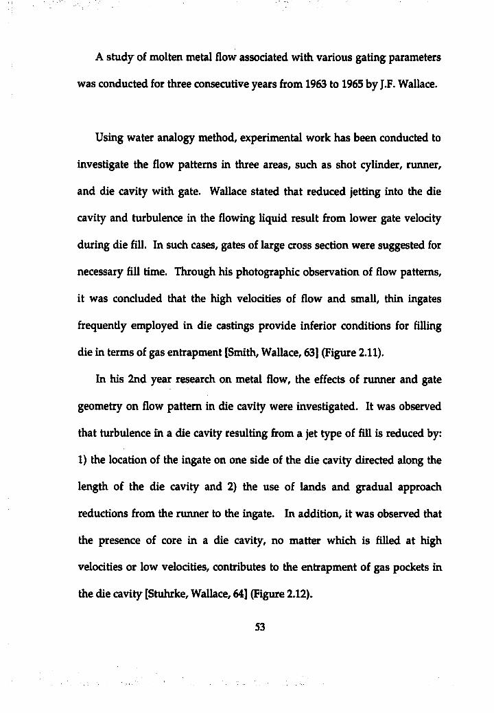
A study of molten metal flow associated with various gating parameters

was conducted for three consecutive years from 1963 to 1965 by J.F. Wallace.

Using water analogy method, experimental work has been conducted to

investigate the flow patterns in three areas, such as shot cylinder, runner,

and die cavity with gate. Wallace stated that reduced jetting into the die

cavity and turbulence in the flowing liquid result from lower gate velocity

during die fill. In such cases, gates of large cross section were suggested for

necessary fill time. Through his photographic observation of flow patterns,

it was concluded that the high velocities of flow and small, thin ingates

frequently employed in die castings provide inferior conditions for filling

die in terms of gas entrapment [Smith, Wallace, 63] (Figure 2.11).

In his 2nd year research on metal flow, the effects of runner and gate

geometry on flow pattern in die cavity were investigated. It was observed

that turbulence in a die cavity resulting from a jet type of fill is reduced by:

1) the location of the ingate on one side of the die cavity directed along the

length of the die cavity and 2) the use of lands and gradual approach

reductions from the runner to the ingate. In addition, it was observed that

the presence of core in a die cavity, no matter which is filled at high

velocities or low velocities, contributes to the entrapment of gas pockets in

the die cavity [Stuhrke, Wallace, 64] (Figure 2.12).

53

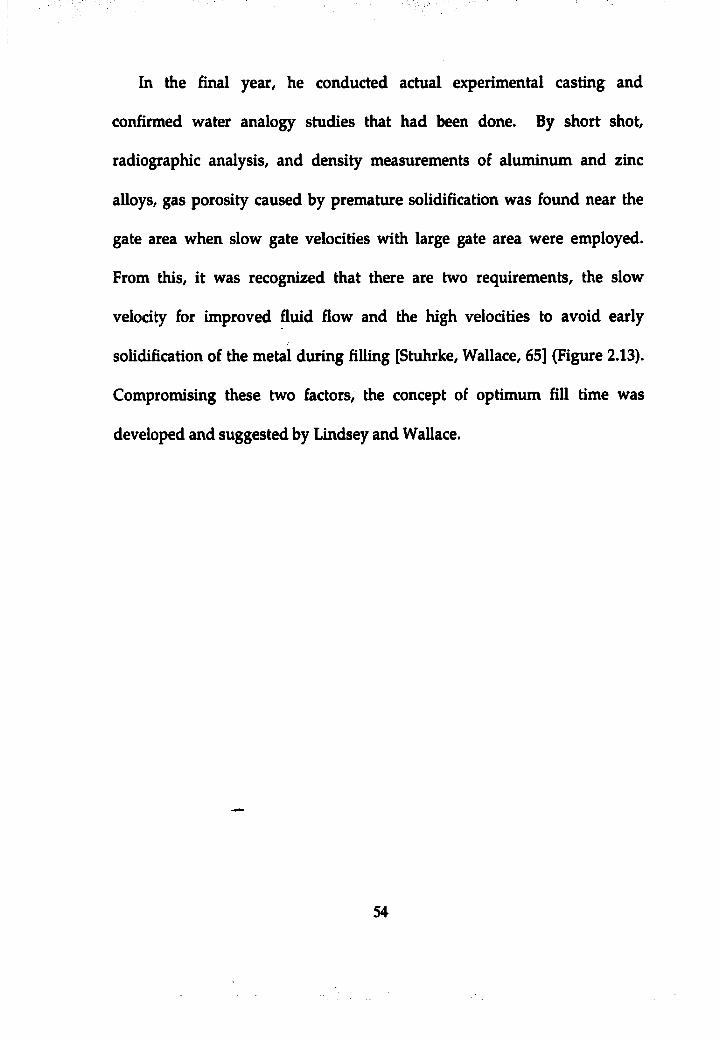
In the final year, he conducted actual experimental casting and

confirmed water analogy studies that had been done. By short shot,

radiographic analysis, and density measurements of aluminum and zinc

alloys, gas porosity caused by premature solidification was found near the

gate area when slow gate velocities with large gate area were employed.

From this, it was recognized that there are two requirements, the slow

velocity for improved fluid flow and the high velocities to avoid early

solidification of the metal during filling [Stuhrke, Wallace, 65] (Figure 2.13).

Compromising these two factors, the concept of optimum fill time was

developed and suggested by Lindsey and Wallace.

54

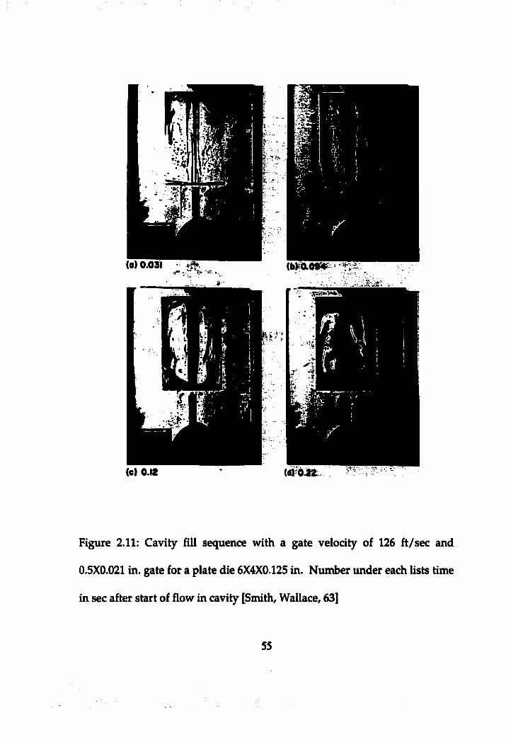
( 0 ) 0 . 0 3 1 - ft- '-P . . .(bKOiO#

(e) 0.12 (dKOjZ

Figure 2.11: Cavity fill sequence with a gate velocity of 126 ft/sec and

0.5X0.021 in. gate for a plate die 6X4X0.125 in. Number under each lists time

in sec after start of flow in cavity [Smith, Wallace, 63]

55

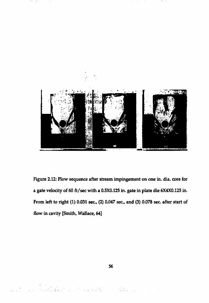
Figure 2.12: Flow sequence after stream impingement on one in. dia. core for

a gate velocity of 60 ft/sec with a 0.5X0.125 in. gate in plate die 6X4X0.125 in.

From left to right (1) 0.031 sec., (2) 0.047 sec., and (3) 0.078 sec. after start of

flow in cavity [Smith, Wallace, 64]

56

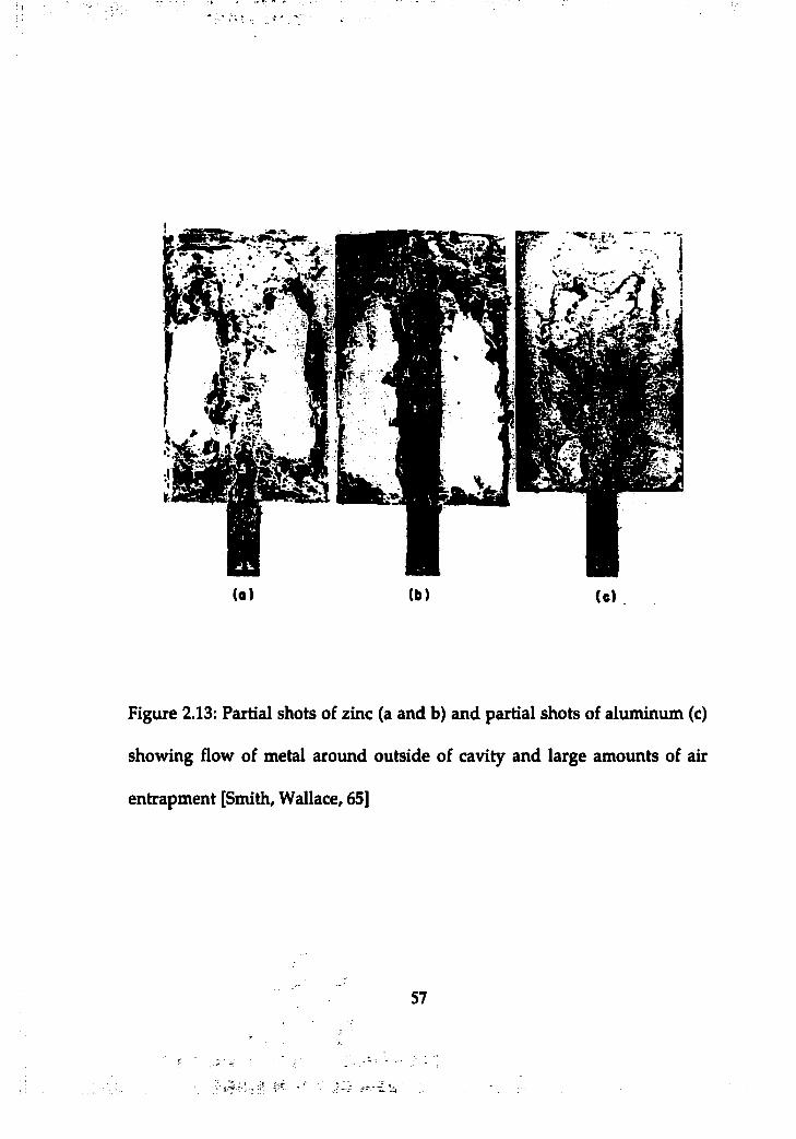
(0 ) (b) (e)

Figure 2.13: Partial shots of zinc (a and b) and partial shots of aluminum (c)

showing flow of metal around outside of cavity and large amounts of air

entrapment [Smith, Wallace, 65]

57

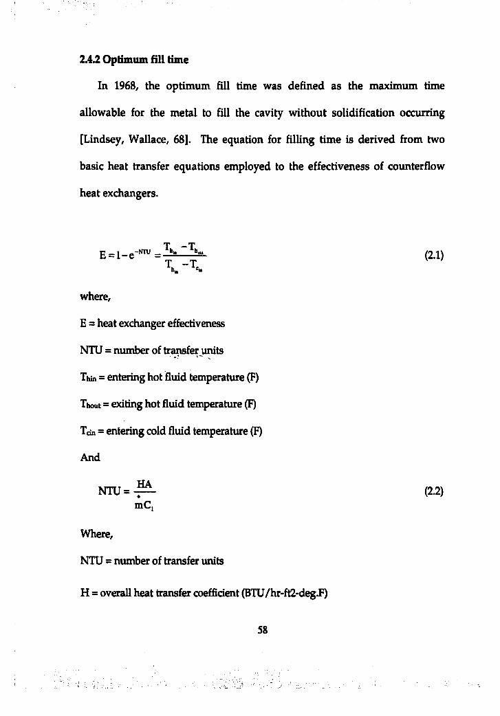
2A2 Optimum fill time

In 1968, the optimum fill time was defined as the maximum time

allowable for the metal to till the cavity without solidification occurring

[Lindsey, Wallace, 68]. The equation for filling time is derived from two

basic heat transfer equations employed to the effectiveness of counterflow

heat exchangers.

E = l - e ~ ^ (2.1)T - T

where,

E = heat exchanger effectiveness

NTU = number of transfer units

Thin = entering hot fluid temperature (F)

Thout = exiting hot fluid temperature (F)

Ton = entering cold fluid temperature (F)

And

N T U = - ^ (2.2)mC,

Where,

NTU = number of transfer units

H = overall heat transfer coefficient (BTU/hr-ft2-degJ0

58

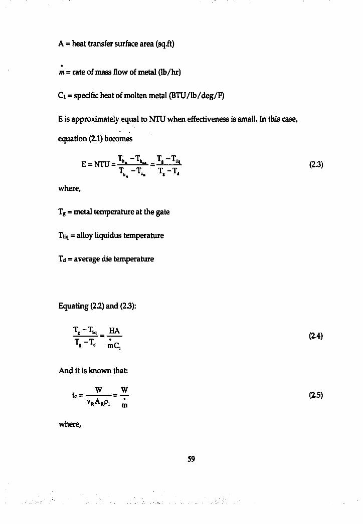
A = heat transfer surface area (sq.ft)

m = rate of mass flow of metal (lb/hr)

Cl = specific heat of molten metal (BTU/lb/deg/F)

E is approximately equal to NTU when effectiveness is small. In this case,

equation (2.1) becomes

T T TE = NTU = i i (2.3)

t , - t,

where,

Tg = metal temperature at the gate

Thq = alloy liquidus temperature

Td = average die temperature

Equating (2.2) and (2.3):

^ = (2.4)mCi

And it is known that:

t c = - ^ = ^ (2.5)VrArP, m

where.

59

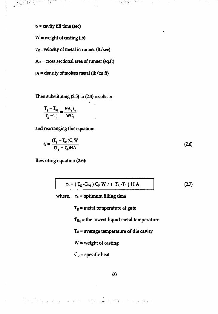
te = cavity fill time (sec)

W = weight of casting (lb)

VR =velocity of metal in runner (ft/sec)

Ar = cross sectional area of runner (sq.ft)

Pi = density of molten metal (lb/cu.ft)

Then substituting (2.5) to (2.4) results in

T, -T ^ HA,t,T ;-T , WC,

and rearranging this equation:

(T,-T^)C,W' (T,-TJH A

Rewriting equation (2.6):

To = ( T g - I u q ) C p W / ( T g - T d ) H A

(2.6)

(2.7)

where. To = optimum filling time

Tg = metal temperature at gate

Tuq = the lowest liquid metal temperature

Td = average temperature of die cavity

W = weight of casting

Cp = specific heat

6 0

H = overall heat transfer coefficient

A = surface area of casting

A careful analysis of . the data indicated that the value for the ratio of

thermal conductivity over the thickness of the oxide-lubricant layer was

found to be 0.44 BTU/sq,ft/Fi Substituting the appropriate values for

aluminum and zinc alloys to equation (2.7) results in:

r r -T„ )WAluminum alloys: To = 0.59 — — - — (2.8)

(T, -T JA ,

rr -T., iwZinc alloys: To =0.28 (2.9)

(T ,-T JA ,

From these two equations, the optimum cavity fill time for aluminum and zinc

alloys can be calculated [Kitting, 00].

This theoretically developed equation was investigated by experiments

as well. Through experiments, it was shown that calculated optimum fill

time curve is similar to the distribution of experimental fill time determined

by quality of surface finish produced and given condition set up with

assumptions of Cp =0.259 Btu/lb.deg.F and Tuq = 1090 deg.F for A1 380

[Lindsey, 68]. This result implies that the above optimum fill time equation

61

provides somewhat conservative criteria being focused only on surface

quality, which might not allow any solid fraction. In addition, the pay-off of

the amount of air entrapment to obtain good surface quality was not

investigated and the criterion of surface quality was not clearly defined.

In 1972, Wallace introduced three different types of jet flow with the

high-speed motion pictures of flow patterns using actual molten metal of A1

380 and Zinc alloy, Zamak 3. The types are continuous jet flow at low

velocities, coarse particle jet flow at intermediate velocities, and atomized

particle jet flow at high velocities (Figure 2.14). Based on these three

different types of jet flow, suggested optimum fill time and maximum fill

time was investigated and presented in terms of surface quality of

experimental castings [Deporto, 72] (Figure 2.15). By this investigation and

results, it was found that the type of jet flow is one of important parameters

of optimum fill time, which implies that heat transfer rate between the die

and molten metal changes by different jet types of flow, such as continuous,

coarse, and atomized jet flow [Maier, 75].

62

2.4.3 Atomized flow

For the investigation of the relative importance of physical parameters

(inertial, surface tension, and viscous forces) to the types of jet flow,

Onesorge tried to classify photographic data of liquid jets of water, oil,

glycerin, and aniline. He employed three different dimensionless numbers

for the analysis: Reynolds number (R), Weber number (W), and the Z

number. Reynolds number represents the ratio of inertial forces to viscous

forces, Weber number stands for the ratio of inertial forces to surface tension

forces, and Z number is defined as the ratio of viscous forces to surface

tension forces [Maier, 75].

where,

(i = fluid viscosity

p = fluid density

o = fluid surface tension

abd = orifice diameter=2-a+b

a = gate widdi

63

b = gate thickness

Based on his experiment, he constructed the plot of log Z vs. log R. (Figure

2.16) It can be seen here that the plot can be divided into three regions. At low

Reynolds number zone I, continuous flow occurs because the stream would not

break up before it impinged the cavity wall. At medium Reynolds number zone

U, the stream appeared to break up into larger particles. At high Reynolds

number, zone III, fine particles or atomized streams are produced.

Under the assumptions that surface tension, viscosity, and density are

substantially constant in the temperature range, Onesorge found that

atomization of jet flow results hrom increasing jet velocity, hydraulic

diameter, and density and decreasing viscosity and surface tension [Maier,

75].

Once flow was atomized, the atomized stream expands laterally to a

greater extent compared to coarse particle flow because more turbulent

metal stream has a larger radial component of velocity [Maier, 75]. The

lateral expansion of atomized flow might be desirable to achieve relatively

uniform filling compared to solid jet flow in die cavity. In 1966, Veinik

stated that atomized cavity fill generates uniformly dispersed pores in the

cavity and good surface quality accordingly [Veinik, 66].

64

However, atomization is favored by high velocities of flow and the high

velocity causes both die erosion and more turbulent flow of metal with higher

Reynolds number, which increases overall air entrapment (amount of global gas

porosity) in die cavity even if atomized fill generates relatively uniform porosity

distribution and relatively good surface quality. One of North America Die

Casting Association (NADCA) reports states "Most die castings are made with

the same methods used for years, which involves atomized flow. This results in

gas entrapment and castings that have a hard time passing the blister test"

[NADCA, 971.

On the other hand, in different industry point of view, the well-developed

atomized flow has an important role in producing relatively thin castings (e.g.

electronic devices) in spite of the disadvantages regarding air entrapment.

Unlike making die castings thicker and bigger to replace steel and iron

components, such as automobile parts, making die castings thinner and lighter to

replace polymer components, such as electronic or communication devices can

not avoid high speed filling, which may cause atomized flow [Hao, 98].

65

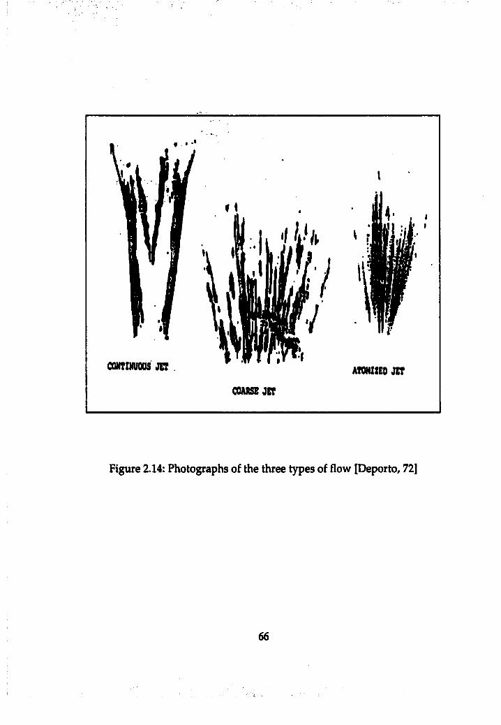
/CONTINUOUS JET

COARSE JET

! I

ATOMIZED JET

Figure 2.14: Photographs of the three types of flow [Deporto, 72]

66

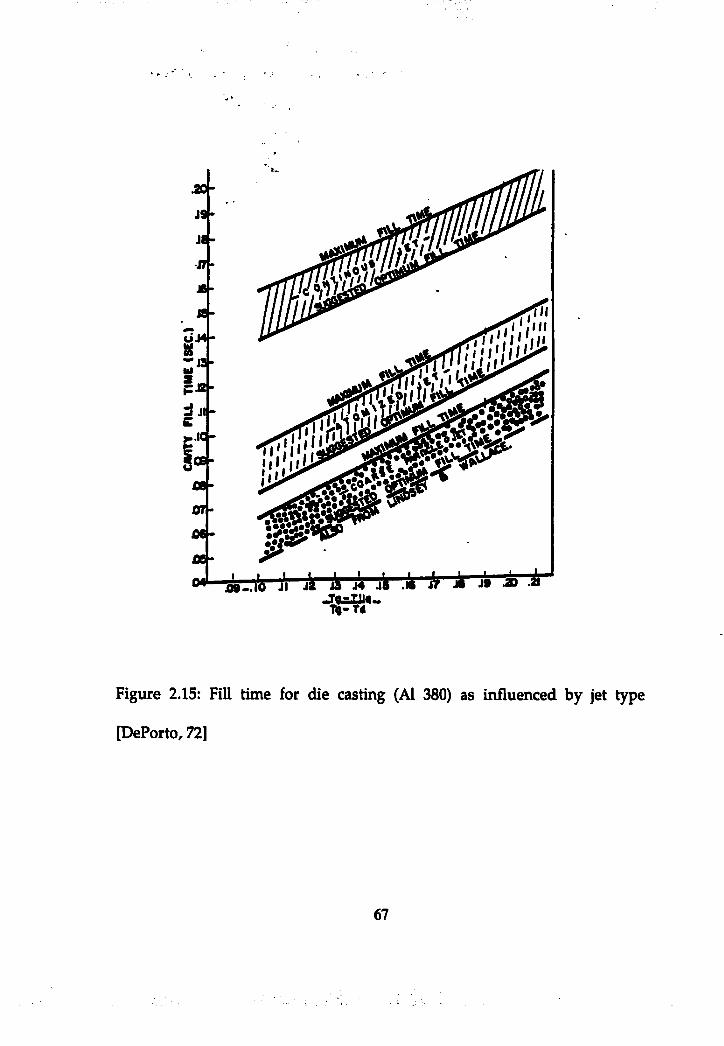
.20-

J 9 -

J l -

J7

JB

is l -

■;

3 W

0*" x » . . l 'ô J l A A J 4 J 8 . i

i M : ' "

J t J 9 .20 .21

Figure 2.15: Fill time for die casting (A1 380) as influenced by jet type

[DePorto, 72]

67

(§)

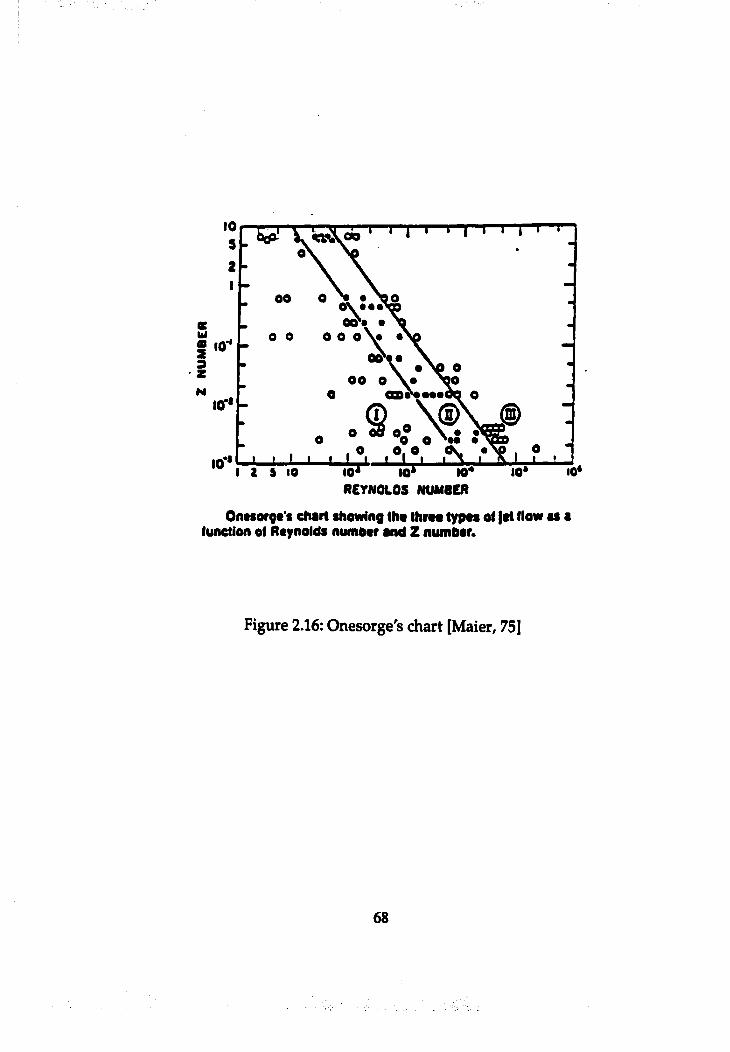
I 2 » 10 10* 10* Mr*REYNOIOS NUMBER

Ontsorgt's chart showing tho Ihroo typos of (at flow as a function of Reynolds numbar and Z numbar.

Figure 2.16: Onesorge's chart [Maier, 75]

68

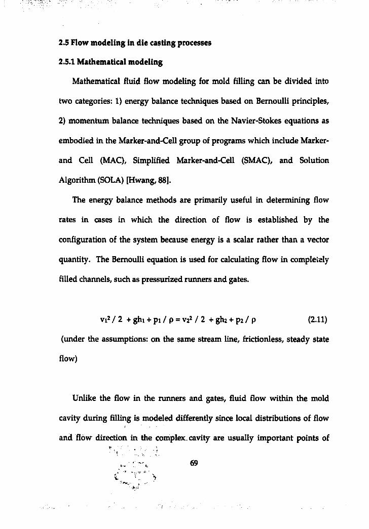
2.5 Flow m odeling in die casting processes

2.5.1 Mathematical m odeling

Mathematical fluid flow modeling for mold fllling can be divided into

two categories: 1) energy balance techniques based on Bernoulli principles,

2) momentum balance techniques based on the Navier-Stokes equations as

embodied in the Marker-and-Cell group of programs which include Marker-

and Cell (MAC), Simplified Marker-and-Cell (SMAC), and Solution

Algorithm (SOLA) [Hwang, 88].

The energy balance methods are primarily useful in determining flow

rates in cases in which the direction of flow is established by the

configuration of the system because energy is a scalar rather than a vector

quantity. The Bernoulli equation is used for calculating flow in completely

filled charmels, such as pressurized runners and gates.

vi2 / 2 + ghi + pi / p = V2 / 2 + ghz + p2 / p (2.11)

(under the assumptions: on the same stream line, fiictionless, steady state

flow)

Unlike the flow in the runners and gates, fluid flow within the mold

cavity during filling is modeled differently since local distributions of flow

and flow direction in the complec cavity are usually important points of

69

interest. For the calculation of velocity vectors and locations of fluid

including front flow inside the cavity, mass and momentum balance

methods including free surface calculation are necessary.

The conservation equations for mass and momentum are complex

equations, which are non-linear, coupled, and difficult to solve. Experience

shows that the Navier-Stokes equations describe the flow of a Newtonian

fluid accurately. Only in a small number of cases - mostly fully developed

flows in simple geometries, e.g. in pipes, between parallel plates etc. - is it

possible to obtain an analytical solution of Navier-Stokes equations

[Ferziger, 96].

In all cases in which such an analytical solution is possible, many terms

in the equations are zero. Some terms are unimportant and we may neglect

them even though this simplification introduces an error. In most cases,

even the simplified equations can not be solved analytically; one has to use

numerical method.

Incompressible flow model

In molten metal flow, the fluid density may be assumed constant. In

addition, if the flow is assumed to be isothermal (rapid fill time), viscosity is

also constant.

70

The basic governing equations for 2D isothermal fluid flow are as

follows:

1) Continuity equation: (density p = const. )

( 3 u / a k ) + ( a v / a y ) = o (2.12)

2) Momentum equations (Navier-Stokes Equation): When fluid is

Newtonian fluid with constant density and viscosity

p [(au/at) + (uau/ax) + (vau/ay)]

= - (ap/ax) + p [ (a2u/ax2) + (a^u/ay:) 1 (2.13)

p [(av/at) + (uav/ax) + (vav/ay)i

= - (ap/ay) + p [ (d^v/dx^) + (a^v/ayZ) 1 +pg (2.14)

where, u, v: velocity in x, y direction, p: pressure, p: density, p: dynamic

viscosity, g: gravity force

71

Creeping flow m odel

When flow velocity is very small, the fluid is very viscous, or the

geometric dimensions are very small (i.e. when the Reynolds number is

small), the convective terms in the Navier-Stokes equations play a minor role

and can be neglected. The flow is then dominated by the viscous, pressure,

and body forces and is called creeping flow. The momentum balance

equation is then:

(8p/8x) = \i [ (82u/8x2) + (82u/8y2) ] (2.15)

(8p/8y) = p [ (82v/8x2) + (82v/8y2) ] +pg (2.16)

where,

u, V: velocity in x, y direction,

p: pressure,

p: density,

p: dynamic viscosity,

g: gravity force

This model can be used for gravity castings or injection molding.

72

2.5.2. Computer modeling of cavity flow

Fluid modeling using computers is not only the most economical and

practical way to get information of physical phenomena, but also it is the

often only feasible way [Hwang, 88].

For cavity flow analysis, the most common technique for numerical

modeling of cavity flow is the family of computational techniques called

MAC, SMAC, and SOLA-VOF (Solution Algorithm-volume of fluid) dealing

with free surface in addition to continuity and momentum balance

equations.

The Marker-And-Cell (MAC) technique developed in 1965 by F.H.

Harlow and J.E. Welch [Harlow, '65] is one of the numerical techniques for

determining fluid flow patterns. The MAC uses the finite difference based

numerical method for predicting "Time dependent viscous incompressible

fluid flow with free surface".

MAC first divides the system into number of subdivisions, called cells,

which are usually rectangular. Then set of imaginary markers is introduced

into the system to represent the location of fluid at any instant. The velocity

field of moving fluid domain can be calculated by the application of fluid

dynamic principles. Next, the markers are moved according to the

calculated velocity field in order to represent new location of fluid domain.

73

This procedure can be repeated from the beginning when the cavity is empty

until it is completely filled.

For the calculation of velocity field in moving molten metal, two

different regions should be considered. Those are the interior region and

surface region. In the interior region, the principle of mass conservation,

momentum conservation and finite difference technique are used. In the

surface region, however, the mass conservation principle is not valid

because the mass within the cells of the surface region is changing. Instead,

free surface boundary conditions should be obeyed, which is the stress

condition on the free surface. The stress condition is a tangential stress

condition, which should vanish on the free surface and normal stress

condition which should balance the applied pressure plus the surface

tension.

The simplified MAC method (SMAC) was developed to avoid the

problem that MAC has. The problem is the complexity in programming due

to the necessity of simultaneous calculation of the momentum and pressure

equations. In the SMAC method, the pressure does not need to be explicitly

calculated. The only thing that must be considered is the velocity

components and the boundary conditions at the free surface and the solid

wan. .

V - ' 7 4

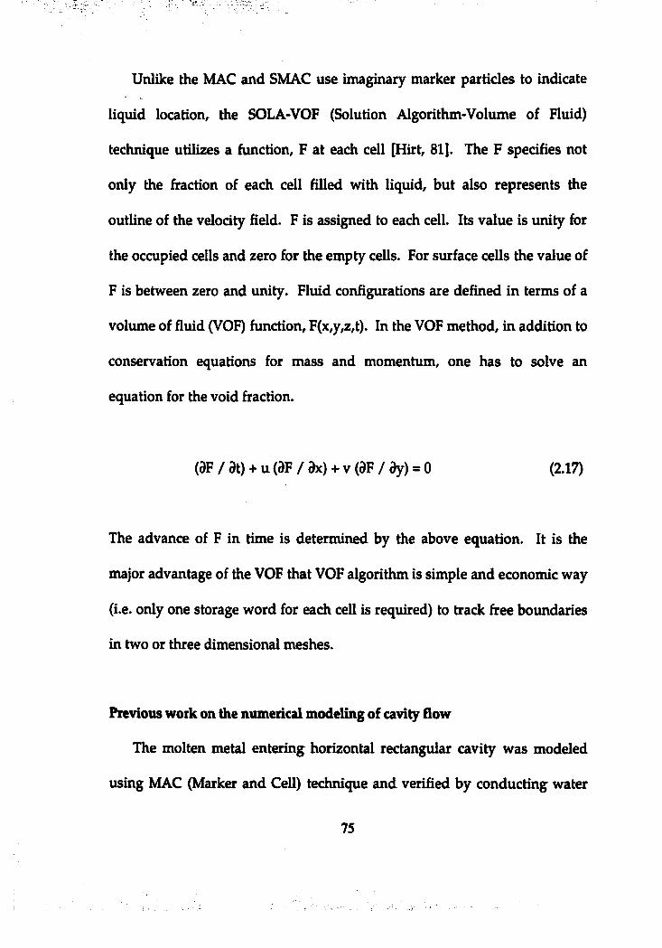
Unlike the MAC and SMAC use imaginary marker particles to indicate

liquid location, the SOLA-VOF (Solution Algorithm-Volume of Fluid)

technique utilizes a function, F at each cell [Hirt, 81]. The F specifies not

only the haction of each cell filled with liquid, but also represents the

outline of the velocity field. F is assigned to each cell. Its value is unity for

the occupied cells and zero for the empty cells. For surface cells the value of

F is between zero and unity. Fluid configurations are defined in terms of a

volume of fluid (VOF) function, F(x,y,z,t). In the VOF method, in addition to

conservation equations for mass and momentum, one has to solve an

equation for the void fraction.

OF / at) + u (3F / ax)+ V (aF / ay)= o (2.17)

The advance of F in time is determined by the above equation. It is the

major advantage of the VOF that VOF algorithm is simple and economic way

(i.e. only one storage word for each cell is required) to track firee boundaries

in two or three dimensional meshes.

Previous work on the numerical modeling of cavity flow

The molten metal entering horizontal rectangular cavity was modeled

using MAC (Marker and Cell) technique and verified by conducting water

75

analog test [Hwang, 83]. In l987, ÿiey developed another cavity fill model of' t i

'three spoke wheel'Using-SOLA-VOF algorithm and very good agreement

between water analog test results and numerical model was observed.

In addition to Hwang's modeling, models using MAC algorithm have

been developed and investigated [Han, 89], [Chen, 91], [Lee, 95]. Han

modeled the flow patterns using different gates with which Wallace

conducted water analog test in 1965 and compared the simulation results

with the picture from water model. Cavity filling with core was modeled by

Chen and the active movement of flow front due to the rigid obstacles

(cores) was investigated using SMAC algorithm. In 1993, using modified

SMAC technique based on finite difference method including turbulence

model, Lee modeled cavity fill patterns and investigated the effect of wall

thickness. His numerical model was verified by water analog test and good

agreement between two results was achieved. He concluded that the fluid

computational technique, based on finite difference method, has the

capability of dealing with the transient flow with firee surface occurring

during cavity filling.

With the MAC method, the SOLA-VOF technique based on finite

difference method has been widely used for numerical cavity flow modeling

[Domanus, 86], [Iwata, 91], [Kallien, 92], [Hwang, 93], [Schmid, 95], [Yuan,

97]. Iwata developed two-dimensional model of cavity fill (disk plate) to

76

investigate the air entrapment due to filling patterns employing various

gates. It was claimed that the numerical model was used successfully for gas

defect analysis and the defects could be decreased in actual castings

applying the results of the analysis.

Flow3D®

A commercial package, Flow3D, which is an extension of the SOLA

[Hirt, 75] and SOLA-VOF [Nichols, 80] family of free surface modelers has

superior mold filling modeling capability. It has superior free surface

modeling capability, which allows the handling of free surface breakup,

unlike many other models, which assume continuous free surfaces. Flow3D

is therefore capable of handling the complicated free surface movement

caused by jetting, flow separation [Venkatesan, 93].

Flow3D has been used with some success for the mold filling simulation

[Hong, 97], [Masuda, 95], [Righi, 95]. The simulation results of Flow3D were

compared with water analogy results showing similarity between two

results from Flow3D and water analog test, and validity of the program

accordingly [Venkatesan, 95], [Barkhudarov, 93] (Figure 2.17).

Flow3D is evolved from the Marker-and-Cell (MAC) [Harlow, 65] finite

difrerence techniques, which uses pressure and velocity as primary dependent

77

variables. This pro^am calculates dynamics of fluids in three space dimensions

and is an extension, to &e SOLA-VOF programs with several additional features

[Barkhudarov, 93].

The numerical approximations of mass continuity and momentum

equations are performed by assuming that the flow region is divided into a

mesh of fixed rectangular cells. All variables are located at the centers of the

cells except for the velocities, which are at the cell faces.

Most terms in the equations are evaluated using the current time-level

values of the local variables, i.e., explicitly, although various implicit options

exist as well. This produces a simple and efficient computational scheme for

most purposes but requires the use of a limited time-step size to maintain

computationally stable and accurate results. One exception to this explicit

formulation is in the treatment of pressure forces. Pressures and velocities

are coupled implicitly by using time-advanced pressures in the momentum

equations and time-advanced velocities in the continuity equation. This

semi-implidt formulation of the finite difference equations allows for the

efficient solution of low speed and incompressible flow problems. However,

semi-implidt formulation results in coupled sets of equations that must be

solved by an iterative technique.

78

In Flow3D, back-presstiie effect in cavi^ can be modeled using adiabatic

bubble model, which is very useful especially for flow pattern analysis in die

cavities. The bubble model evaluates the pressure P in each void region based on

the void region volume V using isentropic model of expansion or compression in

which PV is constant assuming that the void region behaves as a perfect gas.

However, a drawback of this adiabatic bubble model is based on the assumption

that gas in the die cavity is completely trapped in the die cavity, which is not

always true. Unless vents are not closed by molten alloy, gas escapes out of the

die cavity through the vents.

79

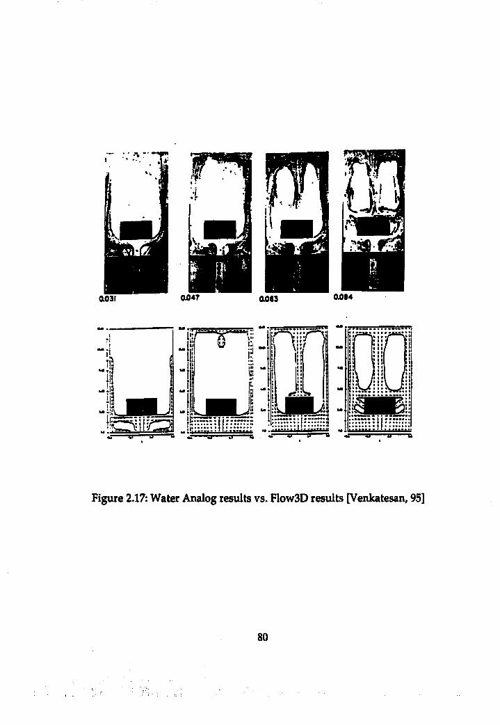
ao3i 0A47 a063 0094

r ^ i -

«1 4J

Figure 2.17: Water Analog results vs. Flow3D results [Venkatesan, 95]

80

' ' i j ' ' / ' - : ' ■ . r >■ - •■ : . ' V / T i : ’ i j

»v;, ' '::2.5.3 Water m odeling

The water a n a lo g mèüiods in conjunction with photographic techniques

have long been considered a useful method to analyze flow patterns within

the gating system and die cavities. Even though the water model analogy

method can not be used to evaluate the effect of temperature and partial

solidification of molten metal in die castings, the method is very useful for

analyzing and predicting the direction and path of molten metal flow and air

entrapments in the gating system and cavity (Figure 2.10,2.11, and 2.12).

For proper physical modeling, the flow model must have dynamic similarity

to actual flow systems. Generally, in modeling of free surface flow, which is

cavity flow, forces due to gravity, viscosity and surface tension need to be

considered. For the similarity of the above three physical properties, three

different dimensionless numbers, such as Reynolds number, Froude number,

and Weber number are taken into account [White, 79].

Froude number needs to be equal to have similarity in gravitational forces

[Nguyen and Carrig, 86]. This number expresses the effect of the force of gravity

on the fluid:

F r =— (2.18) (gD):

where.

81

V = mean velocity of flow

g = gravitational acceleration

D = channel mean diameter

To have similarity in viscous forces, the Reynolds numbers (Re) have to be

equal. The Reynolds number is the ratio of inertial forces to viscous forces:

R e = £ ï 2 = f (119)K

where, in addition to previous symbols

p = density of fluid

p = dynamic fluid viscosity

K= p/p= kinematic fluid viscosity

To have both model and actual Reynolds and Froude numbers equal, both

equations (2.18) and (2.19) can be modified to obtain [Kiting 00]:

D .

L°PJ

3

"=D, I (2.20)

where.

Dr= length scale ratio

Dm = model hydraulic mean diameter

Dp = actual part hydraulic mean diameter

. ' 8 2

Km - model kinematic viscosity

Kp = actual part kinematic viscosity

From equation 2.20, it can be seen that if model is the same size as actual

system then Dr = 1. It means then the kinematic viscosity of both model and

actual system have to be the same in order to satisfy the requirements of Froude

and Reynolds numbers.

To have a complete similarity, the force due to surface tension needs to be

considered. The Weber number (We), which describes the ratio of inertia forces

to surface tension forces, is used here.

Q21)

where,

V = mean flow velocity D = orifice diameter

p = fluid density o = surface tension

In water analog, water is used as a replacement for the aluminum alloy

and is delivered into transparent mold to predict the flow of molten alloy.

Therefore, the effects of difference in physical properties between water and

molten alloy (aluminum) on flow patterns in die cavity have been

investigated [Wallace, 64], plao, 98]. As can be seen in the table. 2.3,

83

•* i

kinematic viscosity of water and aluminum is almost the same but the

surface tension of water is significantly different from aluminum. For the

study of surface tension effects on the flow, Wallace used and compared

flow patterns of three different fluids- methyl alcohol, water, and mercury.

It was observed that increasing the surface tension of the fluid introduced at

high velocities into die cavity tends to decrease the turbulence to some

degree. However, he concluded that the differences in surface tension of

either molten aluminum or zinc do not significantly affect the flow behavior

correlation.

Based on dynamic similitude in hydraulics, Hao also stated that the

filling process is primarily dependent on the inertial and viscous effects, and

hence gravity effects and surface tension can be generally ignored.

However, he mentioned that surface tension is very important factor if

atomization happens in a jet [Hao, 98].

84

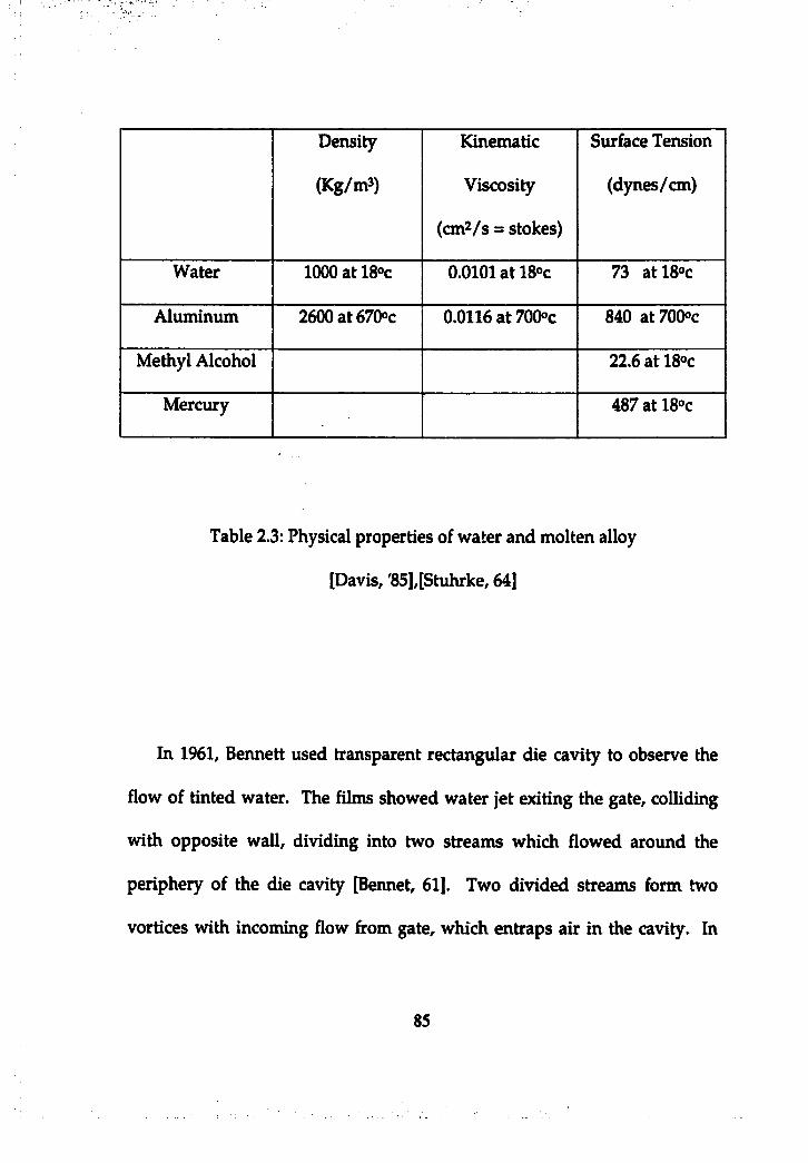
Density

(Kg/m3)

Kinematic

Viscosity

(cmZ/s = stokes)

Surface Tension

(dynes/cm)

Water 1000atl8»c 0.0101 at 18°c 73 atl8»c

Aluminum 2600at670«c 0.0116 a t 700°c 840 at700®c

Methyl Alcohol 22.6 at 18»c

Mercury 487 at 18«c

Table 2.3: Physical properties of water and molten alloy

[Davis, '85],[Stuhrke, 64]

In 1961, Bennett used transparent rectangular die cavity to observe the

flow of tinted water. The films showed water jet exiting the gate, colliding

with opposite wall, dividing into two streams which flowed around the

periphery of the die cavity [Bennet, 61]. Two divided streams form two

vortices with incoming flow ficom gate, which entraps air in the cavity. In

85

addition to cavity flow analysis, Bennet used water analogy methods to

observe flow pattern in shot sleeve and runner system [Bennet, 66]. In shot

sleeve, curling wave formation, which encloses gas, was shown.

Using water analogy methods, jet behavior of flow characteristics in die

cavity was investigated by Nussey [Nussey, 66]. From 1963 to 1965, Wallace

used water analogy methods to study flow patterns in the cavity under wide

variety of conditions (i.e. types of gates, gate locations, and gate velocities)

[Smith, 63], [Stuhrke, 64], [Stuhrke, 65]. To confirm the results of the water

analogy experiments, Wallace also conducted partial shot, radiographic

examination, and density measurements.

Recently, flow study using water analogy conducted by Lindberg,

Davis, and Hao for the investigation of flow regime, filling pattern, and

atomization of flow [Davis, 85], [Lindberg, 91], [Hao, 98].

86

2.6 Previous work in cavity pre-fill

Even though industry has employed pre-hll approaches as a different

cavity HU approach to achieve high quality castings, literatures related to the

cavity pre-fill injection method are limited.

In 1989, Yamamoto and Iwata conducted water analog tests to

investigate effects of injection speed [Yamamoto, 89]. They found that few

gas bubbles generated at low injection speed and higher injection speed

generates more gas entrapment (Figure 2.18). In addition, it was observed

that even fast shot injection of water generates much less gas bubbles when

cavity is partially filled in advance (Figure 2.19).

In 1995 and 1996, Itamura and Yamamoto published their work on the

effects of injection speed on metal flow in die cavity [Itamura, 95], [Itamura,

96]. Like Wallace [Stuhrke, 65] observed earlier that constant slow gate

velocity generates uniform filling (Figure 2.20), which minimize air

entrapment without vortices due to backward filling from top to bottom in

rectangular cavity, they found maximum speed below which no air

entrapment occurred (Figure 2.21). The obtained critical injection speed was

0.5 m /s. Also, they examined another way to obtain uniform filling pattern

in rectangular cavity. The way that they examined was using dual injection

speeds for cavity fill, which was observed in Yamamoto's 1989 paper and is

similar concept to cavity pre-fill process. The dual speed is divided into

87

slow velocity for pre-charge of cavity and fast velocity for the rapid filling.

This method of cavity filling showed uniform filling without air entrapment

caused by back-fill, (Figure 2.22, g) while the filling method could avoid

seriously delayed filling time when using constant (single) slow gate

velocity.

Figure 2-22 shows the effect of the pre-charge height prior to secondary

charge on mold flow using water analog test with fixed slow (i.e. 0.15 m /s)

injection speed for pre-fill, fast injection speed (i.e. 1.6 m /s). As shown in

the figure, both cases of 10 mm and 15 mm pre-charge caused air

entrapments at the bottom of the mold, in contrast to the result of 20 mm

which had no air entrapment. In addition, they investigated the effect of

pre-charge heights (different fast shot transition points from slow to fast) on

the amount of air entrapment (Figure 2.23). By measuring the amount of air

entrapment, the relationship between height of pre-charge and second fast

shot injection speed with fixed slow injection speed (i.e. 0.4 m /s) and fixed

transition time firom slow to fast (i.e. 20ms) was also investigated (Figure

2.24).

Along with industry approaches, the results from Yamamoto's

experimental work on the effects of dual injection speed provides a positive

aspect of pre-fill process in terms of air entrapment in the die cavity.

88

However, the effects of many parameters and their correlation associated

with pre-fill injection method on filling patterns and air entrapment are still

remaining questions. Those parameters are: slow injection speed during the

pre-fill, acceleration rate from slow to fast injection speed, cavity geometry

including gates and vents, and pre-fill percentages (or pre-charged flow

heights). In addition, as Yamamoto's work was for the application of

squeeze casting, the injection speed that they employed for slow injection for

cavity pre-charge (pre-fill) is too low (e.g. 0.15 and 0.4 m /s of gate velocity)

to complete cavity fill without premature solidification.

8 9

-«■< :

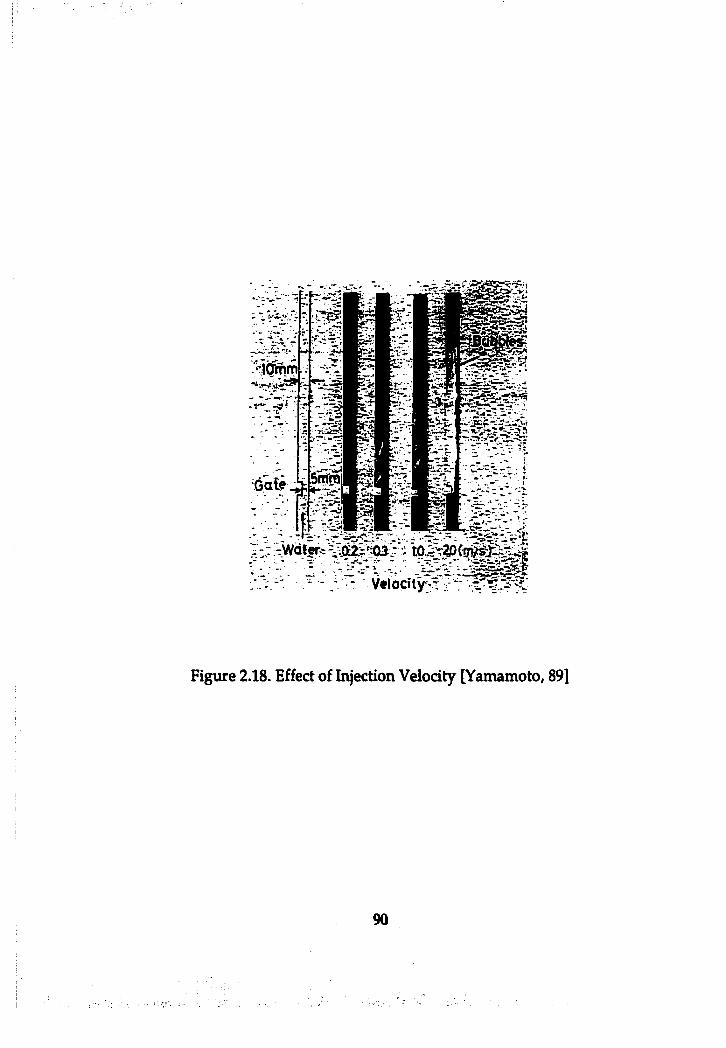
1%:: f é r ^ p i

; 5 -“ - .■ ^ V e lo c i l^ f

Figure 2.18. Effect of Injection Velocity [Yamamoto, 89]

90

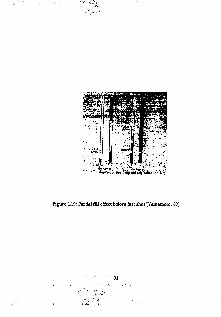
bubblti

•In runnerPoiinon. ol Aginhing Tcsühqf phase -■ -

Figure 2.19: Partial fill effect before fast shot [YamamotO/ 89]

91

. ' r h , ......

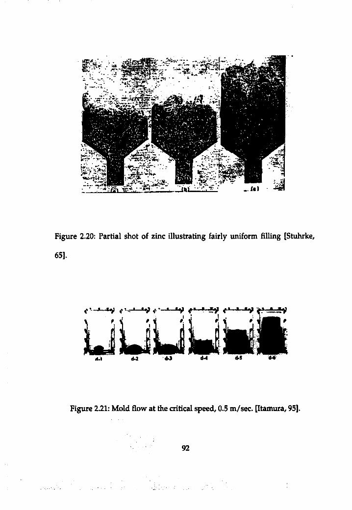
^ ------- - w m# m# ■ - >^#l

K #

:^, .-7 iU -2.V . p '7ir/r:yr-

P i i K b . _ .i* »

Figure 2.20: Partial shot of zinc illustrating fairly uniform tilling [Stuhrke,

65].

— I — ,m

Figure 2.21: Mold flow a t the critical speed, 0.5 m/sec. [Itamura, 95].

92

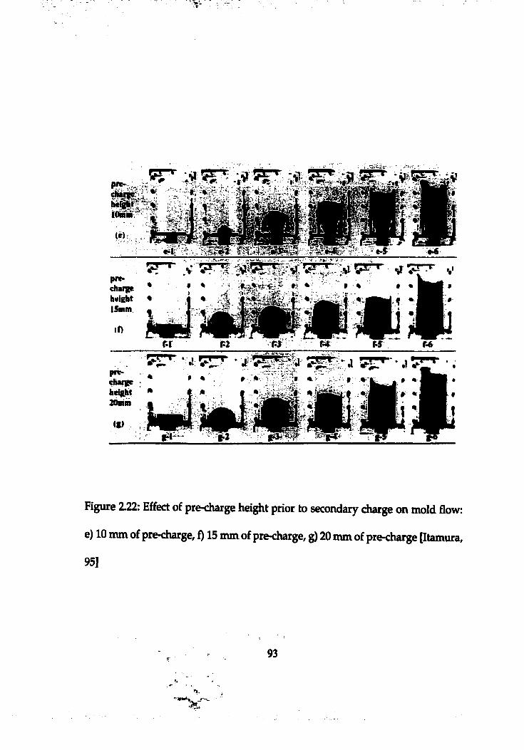
5 ^

« i #

(e>L ,

pre-charpeheîKhr15min

(0

.V ‘ ' 5 ^ ;

« * $ : 1

> r 4 ' '% f

1 -

1 ' l a #

W. .'' '" ' " % " t • h a # »

A r-5 M

piv>cb « itehc fail30nim

(D

• * • * > ..% , t «

Figure 2.22: Effect of pre-charge height prior to secondary charge on mold flow:

e) 10 mm of pre-charge, f) 15 mm of precharge, g) 20 mm of pre-charge [Itamura,

951

93

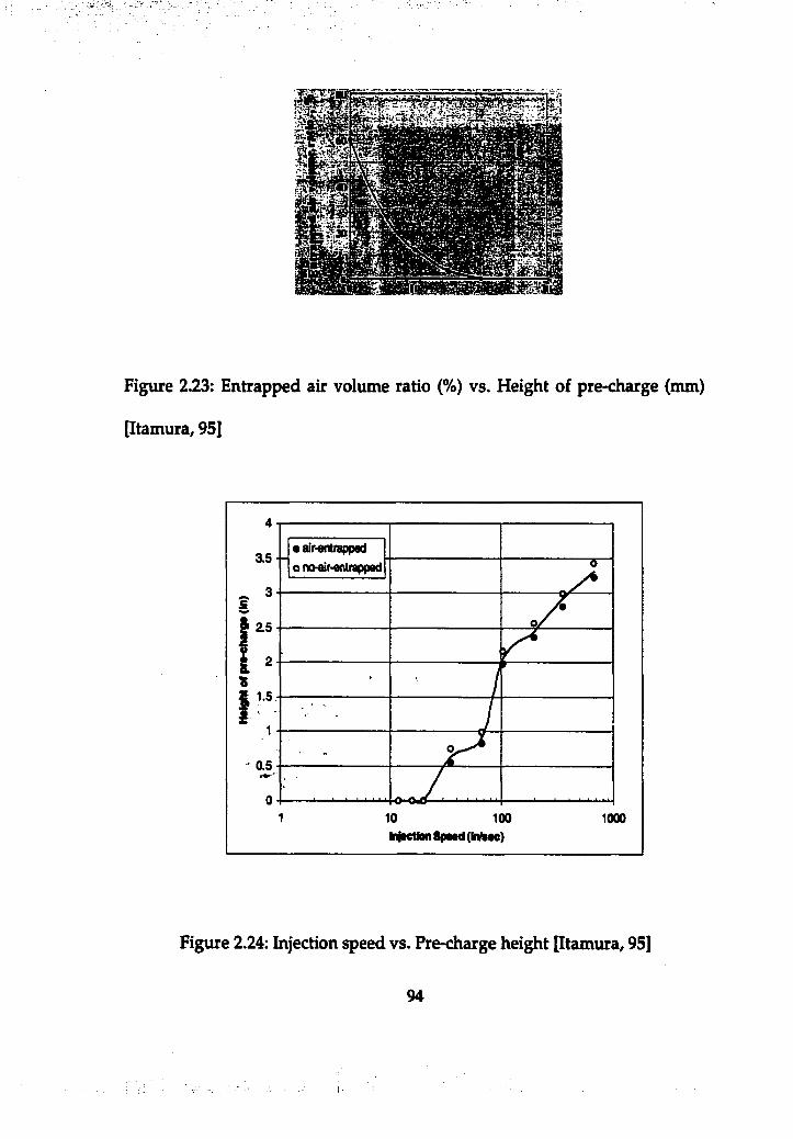
g

Figure 2.23: Entrapped air volume ratio (%) vs. Height of pre-charge (mm)

[Itamura, 95]

a s ■ -

25

- 0.5

10 100 IniKtion SpMd (M «e)

1000

Figure 2.24: Injection speed vs. Pre-charge height [Itamura, 95]

94

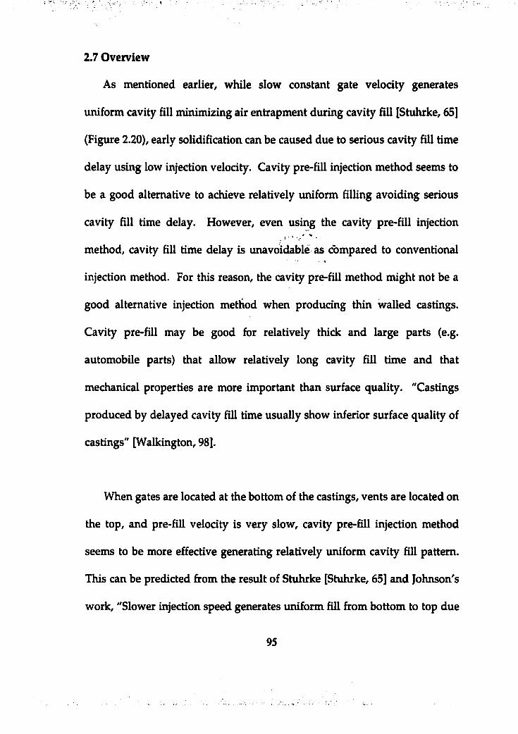
2.7 Overview

As mentioned earlier, while slow constant gate velocity generates

uniform cavity fill minimizing air entrapment during cavity fill [Stuhrke, 65]

(Figure 2.20), early solidification can be caused due to serious cavity fill time

delay using low injection velocity. Cavity pre-fill injection method seems to

be a good alternative to achieve relatively uniform filling avoiding serious

cavity fill time delay. However, even using the cavity pre-fill injection

method, cavity fill time delay is unavoidable as compared to conventional

injection method. For this reason, the cavity pre-fill method might not be a

good alternative injection method when producing thin walled castings.

Cavity pre-fill may be good for relatively thick and large parts (e.g.

automobile parts) that allow relatively long cavity fill time and that

mechanical properties are more important than surface quality. "Castings

produced by delayed cavity fill time usually show inferior surface quality of

castings" [Walkington, 98].

When gates are located at the bottom of the castings, vents are located on

the top, and pre-fill velocity is very slow, cavity pre-fill injection method

seems to be more effective generating relatively uniform cavity fill pattern.

This can be predicted firom the result of Stuhrke [Stuhrke, 65] and Johnson's

work, "Slower injection speed generates uniform fill from bottom to top due

95

to the relatively low inertia force of flow as compared to gravity force". The

flow patterns using different injection speeds and gravity effects on the flow

patterns were investigated using numerical simulations [Johnson, 89] (Figure

2.25). However, if cavity pre-fill injection method is used when gate is

located on the side of casting parts, possible negative effects might be found,

such as alumina surface or flow lines on the castings.

Similarly, as pressure generated by pre-filled fluid might act like an

obstacle to the following incoming flow on the flow path, the inertia of

incoming jet flow seems to be reduced and the direction of the velocity

vector of jet flow seems to be changed. This may be desirable in order to

achieve more uniform cavity fill in the die cavity with complex geometry.

However, the reduced inertia of flow and possible direction changes of jet

flow due to the cavity pre-fill might also cause a negative effect on air

entrapment in some geometries of die cavities. For example, considering

three-dimensional flow expansion effect, cavity fill pattern associated with

casting thickness was investigated [Lee, 95]. In a thin rectangular cavity

with gates at the bottom and vents on the top, the incoming flow hit the both

side walls of cavity and the flow went up to the vents along the both sides

before main stream reached the vents as the direction of partial flow was

toward the both side walls (Figure 2.26).

96

Acceleration rate tirom slow to fast'injection speed in pre-till injection

method might also influence flow patterns in the die cavity as acceleration

influences the inertia of flow. The effect of the acceleration on flow behavior

(wave formation) in the shot sleeve was previously observed [Thome, 95].

97

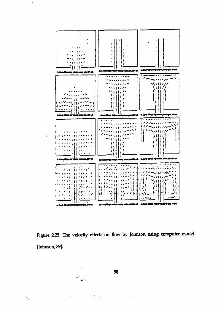
■ • • N V I • f / « » "

'"WX I / /-•'^ \ \ \ l / / '■w\\\I

I / /i n

i l l

I / .

* » I > t I I » ♦ »

— 1

m % % *

. % \‘M\

\\!*

//'■

i;

^\U I / / /

. > ■> > 1 i I I i ’ ; .<•

' C ’.‘ V V \ \ 1 i /■/ / / >■ • ' ' \ \ I I / / '

MX I:: '1

M // '.■I • ■• < • •i/ '.: ;

111 i.i

‘M-M-

I !± !■

1.1 » < \ \ I f / / "'W

\ I'i f ; / / .

Figure 2.25: The velocity effects on flow by Johnson using computer model

[Johnson, 89].

98

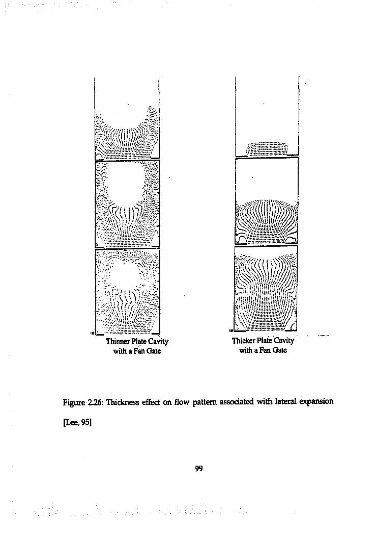
0 # .

m r n n m

Thinner Plate Cavity with a Fan Gate

Thicker Plate Cavity with a Fan Gate

Figure 2.26: Thickness effect on flow pattern associated with lateral expansion

[Lee, 95]

99

CHAPTERS

COMPUTER FLOW MODELING

As a research approach, computer flow models were employed to

Investigate flow patterns and air entrapment when using cavity pre-fill vs.

conventional cavity fill. Computer modeling is cost effective as compared to

the other modeling methods or experimental castings as this research

includes many parametric studies. As a computer-modeling tool, a finite

difference method (FDM) code of FlowSD was used.

3.1 Two dimensional computer flow model

Prior to three-dimensional computer models, two-dimensional computer

flow models were developed using two dimensional test geometry of cavity

to investigate cavity pre-fill effects. This approach reduced the running time

required for computer simulation.

100

3.1.1 Modeling of cavity pre-fill

The model was used to visualize filling patterns in the die cavity using cavity

pre-fill injection method. Figure 3.1 shows schematic shot profiles of cavity

pre-fill. Unlike a conventional shot profile, fast shot starts after the cavity is

partially filled with slow shot velocity in cavity pre-fill approach.

It should be noted that x-axis in shot profile in Figure 3.1 represents

'time', while it usually is 'plunger position' on shot profiles used in industry.

When the x-axis represents plunger position, the shot profile for cavity pre­

fill will be different. The shot (pre-fill) ends at the same point on the x-axis

where conventional shot profile does (Figure 3.4).

101

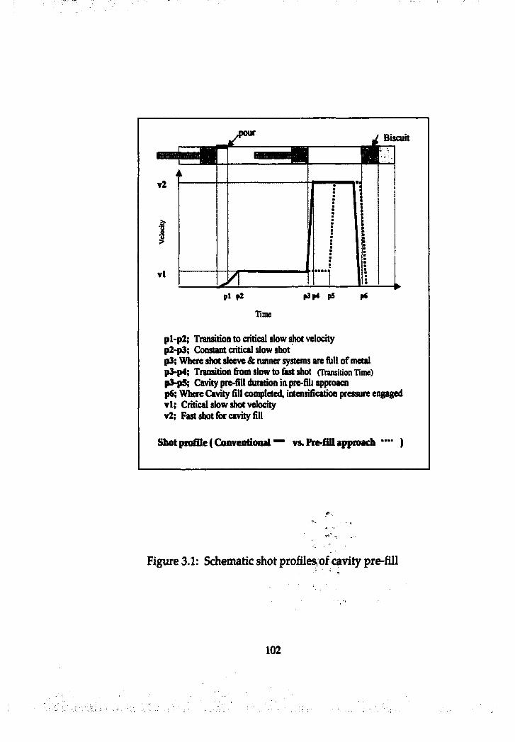
pour

v2

Ivl

Biscuit

mpi p2 p3p4 p5

Time

pl-p2; Transition to critical slow shot velocityp2-p3; Constant critical slow shotp3; Where shot sleeve & runner systems are fiill of metalp3-p4; Transition from slow to first shot (Transition Time)pS'pS; Cavity pre-fill duration in pre-fill approacnp6; Where Cavfry fill completed, intensification pressure engagedv l ; Critical slow shot velocityv2; Fast shot fr>r cavity fill

Shot profile (Omventional‘~ vs. Pite-fill approach ***' )

Figure 3.1: Schematic shot profiles, of cavity pre-fill

102

ùi this computer flow modeling, it was assumed that:

1) Pre-existing air in the die cavity was under the pressure of one

atmosphere (i.e. 1.013 x 10 dyne/cm^),

2) Molten metal flow was viscous and incompressible fluid flow,

3) Air inside the cavity acts as perfect gas, so that equation PV = constant

was applicable for modeling of the back-pressure effect (adiabatic bubble

model in Flow3D: y = 1.4),

4) Molten metal was assumed to be a molten aluminum. The properties of

molten aluminum are constant and based on Smithells Metals References

6th edition, 1983 (e.g. at T=660O, density=2.38 g/cm^, surface tension=914

dyne/cm, dynamic viscosity=0.013 g/cm/sec),

5) Metal injection process in the die cavity was assumed to be adiabatic and

isothermal process in such a short fill time.

6) There was no noise in shot control: shot profile is perfectly linear.

(See schematic shot profiles in Figure 3.1,3.3 and actual shot profile in

Figure 3.4)

An example of 2-D computer flow model

The following is an example of a two dimensional computer flow model

of cavity pre-fill employing: 1) simple rectangular plate cavity, 2) 40% cavity

pre-fill, 3) 10 ms of transition time, 4) 50 cm /s of pre-fill (gate) velocity, and

103

5) fast shot (gate) velocity of 3870 cm/s. The number of meshes is 40 x 40 x 1

(2D). Figure 3.2 is the input file for Flow3D.

Since Flow3D uses a linear interpolation for the velocity between time

points, following inputs for the boundary conditions in Figure 3.2 creates a

shot velocity profile of Figure 3.3.

$bcdata

Wl=2, wr=2, wt=2, wb=6,

timbct(l)=0.0, timbct(2)= 0.188, timbct(3)= 0.198,

wbct(l,5)=50., wbct(2,5)=50., wbct(3,5)=3870.,

Send ' -

Since runners were not included in cavity geometry, the time which fast

shot (transition) starts at was determined by the following method.

timbct(2)=(% pre-fill x cavity area)/(slow shot velocity x gate area) (3.1)

104

5 1

g

wio

Igs>

î;Is .ë

I

IIIIP III IIPIHia

î f-®3

N.® -s a g»:K

i1

I

I?

î

Velocity

V(2)

V(l)

t( l) t(2) t(3)Time

At time t (I)- 0 Vdocity, v(l)=50 cm/s At time, t(2>»0.188, Velocity, v(I)*^0 cra/s At time, t (3)= 0.198, Velocity, v(2)»3870 cm/s

Transition time: 0.198-0.188=0.010=10 ms.

Figure 3.3: A shot profile created by the input of Figure 3.2 in Flow3D

By running this example of input file, the sequence of filling patterns

were described by fluid firaction and velocity vectors every 4 ms firom the

beginning of cavity filling (Figure 3.5).

106

Conventional fill Two different cavity pre-fill(no pie-fiU) shot profile shot profiles

Figure 3.4: Actual shot profiles of cavity pre-fill approach

(Unlike schematic shot profiles in Figure 3.1,' X-axis in this graph is plunger

position)

107

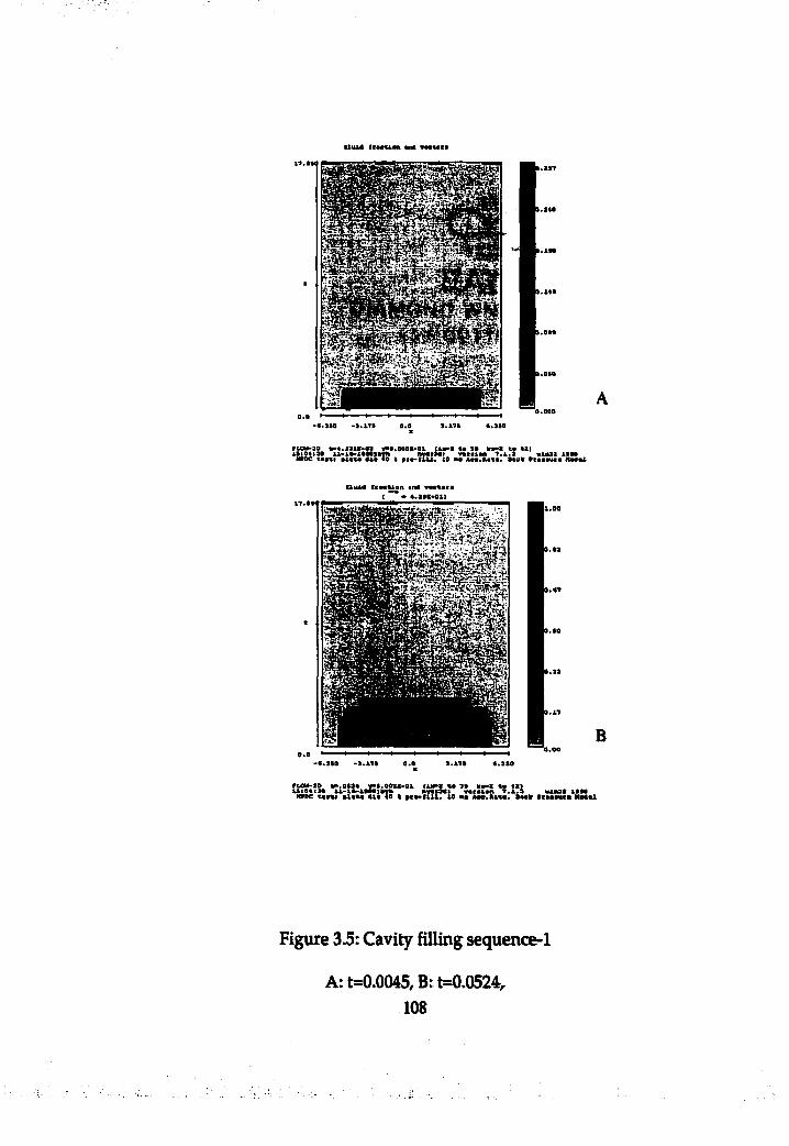
U U iA M t V #*W Km

•«.uo $ w#

CXuM tc « « c io n #m# v«e%#r# t • « .2 M -» 0 1 )

m m mim x ÿ m m

# 3#@ 2 M»

B

Figure 3.5: Cavity filling sequence-1

A:t=0.0045,B:t=0.0524,lOS

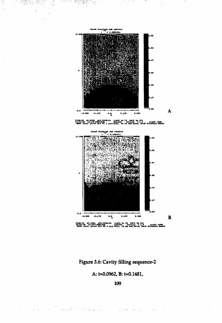
U u i A ( c « c « & o a «fkÉ

m e:;

ruw-3D co.OfM y -t.ooo i-o i. CO a» b«»t m «a>&^Q4*ae ix*xs-t»M 3byn hwic3«t v acsio n 7 .1 .6 winaa i« «

NVDC M act # i# w #1# 40 4 pcs^eX îl» 10 ■■ Aac.R«s«* I t e k tc««M C« Moi

cxuio t c t s u o n 400 v«««oca ( • #.aw*oi)

.. -r

BNaoc ««aot axaca o ia 40 » ac*>c£xi* lO m# A ea.uao a , #aa» tca a a u c a *

Figure 3.6: Cavity M ing sequence-2

A:t=0.0962,B:t=0.1481,

109

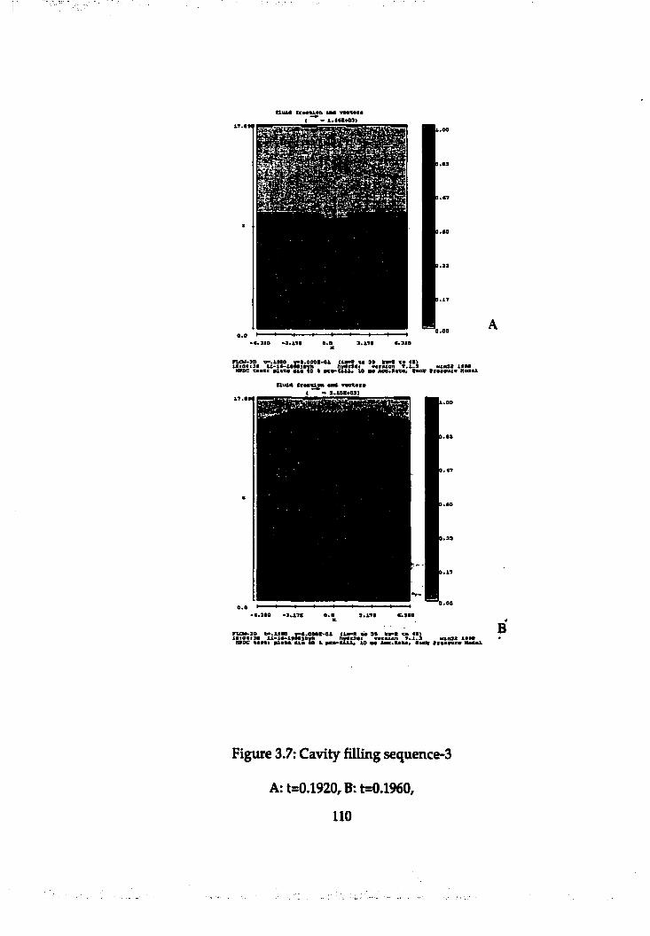
tlu i* «H* v«c«oc«C • l . . « l * 0 9 )

-«.3«0 *9.r7S

ü%?& ’T tiS ît.C îiX "-" «î3«?* ’Î.Æ3! *î.îîi « « , » «ioroe csacr #iw # #i# Io i pc«»uîi« to ## 0#e» icaaaac* Noatx

ttui4 leeettw «M{ a. tot«09i

•t.ate -3*10

iiiîe.Æ»jS«-“ as.?* %.s% *î.îîi ««. »-HOOe «##%* »&•«* é ta Io & p s f t i x t * lO m Aaa.Ka*#^ O m it traaauca W##mi

B

Figure 3.7: Cavity filling sequencers

A:t=0.1920,B:t=0.1960,

110

3.1.2 Cavity pre-fill vs. conventional cavity fill (no pre-fill)

Unlike a previous cavity pre-fill model (Figure 3.5 to 3.7) using 40%

cavity pre-fill, 10 ms transition time, 50 cm /s of pre-fill (gate) velocity, and

3870 cm /s fast shot (gate) velocity, another two dimensional model was

developed using narrower gate width, higher pre-fill velocity (687 cm /s of

gate velocity based on critical slow shot velocity), and lower pre-fill

percentage (20% cavity pre-fill) to see the cavity pre-fill effects on flow

patterns more clearly.

Figure 3.8 shows the difference of flow patterns between using no pre-fill

(conventional cavity fill) and 20% of cavity pre-fill. The difference in flow

patterns in the die cavity was clear. Using cavity pre-fill, back fill effect,

which was observed by many investigators previously, was reduced. It is

obvious that the cavity back fill generates air entrapment in die cavities

when vents are located on the top of the rectangular cavity.

Even though cavity fill-time increased by using cavity pre-fill, a positive

effect of pre-fill was observed. Cavity pre-fill generated more uniform

cavity filling and accordingly less air entrapment in the die cavity. In

addition to percentage cavity pre-fill effect, effects of other related

parameters were investigated in Chapter 3.1.3.

Ill

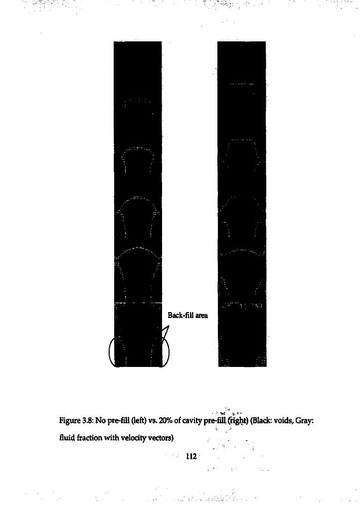
Back-fill area

>*«Figure 3.8: No pre-fill (left) vs. 20% of cavity pre-fill (Black: voids. Gray:

fluid firaction with velocity vectors)

112

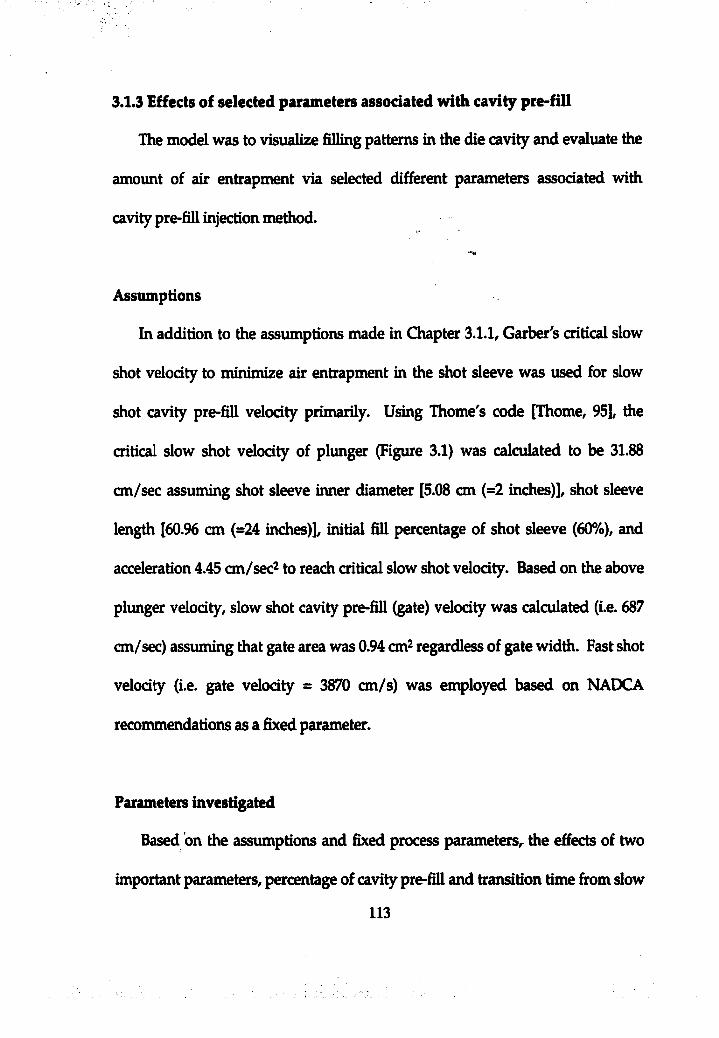
3.1.3 Effects of selected parameters associated with cavity pre-fill

The model was to visualize filling patterns in the die cavi^ and evaluate the

amount of air entrapment via selected different parameters associated with

cavity pre-fill injection method.

Assumptions

In addition to the assumptions made in Chapter 3.1.1, Garber's critical slow

shot velocity to minimize air entrapment in the shot sleeve was used for slow

shot cavity pre-fill velocity primarily. Using Thome's code [Thome, 95], the

critical slow shot velocity of plunger (Figure 3.1) was calculated to be 31.88

cm/sec assuming shot sleeve inner diameter [5.08 cm (=2 inches)], shot sleeve

length [60.96 cm (=24 inches)], initial fill percentage of shot sleeve (60%), and

acceleration 4.45 cm/sec^ to reach critical slow shot velocity. Based on the above

plunger velocity, slow shot cavity pre-fill (gate) velocity was calculated (i.e. 687

cm/sec) assuming that gate area was 0.94 cm^ regardless of gate width. Fast shot

velocity (i.e. gate velocity = 3870 cm/s) was employed based on NADCA

recommendations as a fixed parameter.

Parameters investigated

Based bn the assumptions and fixed process parameters, the effects of two

important parameters, percentage of cavity pre-fill and transition time firom slow

113

to fast shot in cavity pre-fill shot injection method were investigated. The

experimental ranges of two parameters were established based on practices used

in industry [Pribyl, '97], such as 0,10,20,30, and 40% of cavity pre-fill and 10,20,

and 30 milliseconds of transition time. While critical slow shot velocity (i.e. 31.88

cm/sec of plunger velocity) was employed primarily as a slow shot cavity pre-fill

velocity, 70% of the critical slow shot velocity was also employed as a pre-fill

velocity to investigate the effects of cavity pre-fill velocity on air entrapment and

fill patterns (Figure 3.9).

Cavity geometry

To investigate the effects of cavity geometry on filling patterns, two different

geometries of rectangular cavity were employed. One was a simple rectangulâï

plate cavity, 12.7cm x 17.8cm (or 5"x 7') wi& chisel gate and another was a

simple rectangular cavity with four ribs, 1.8cm x 6.4cm (or 0.7'x 2.5"). Two ribs

were on the left wall at the bottom and the other two were on the right side of

wall at the top inside the rectangular cavity, 12.7cm x 17.8cm with chisel gate,

which generates more turbulence of flow in the cavity (Figure 3.10).

In addition, two different widths of gates (wide; 8.9cm (or 3.5") and narrow;

6.4cm (or 2.5"), which are 70% and 50% of cavity width) were also employed to

investigate the effects of gate width on air entrapment and flow patterns in the

die cavity. As mentioned earlier in assumptions, slow shot gate velocity based

114

on critical slow shot plunger velocity were the same even with different gate

widths assuming that gate area was constant (i.e. assuming different gate

thickness with different gate width).

Quantitative analysis of air entrapment

The quantitative analysis of air entrapment in the cavity was possible under

the assumption that vents were the only way for the air in the die cavity to

escape out of the die cavity. The air inside the cavity should be trapped in the

die cavity and the pressure of the air should increase as molten metal is injected

in the cavity as soon as all the vents are closed with molten metal flow. The

amount of air entrapment in the die cavity was estimated by measuring unfilled

cavity volume (% cavity volume) at the moment when all the vents were sealed

with molten metal. Using the above method, when employing different injection

parameters selected, their performances in terms of air entrapment were

investigated (Figure 3.14,3.15,3.16,3.17).

Details about the estimate of air entrapment in computer flow models are

discussed in Chapter 3-3. The estimate was also evaluated using experimental

casting results.

115

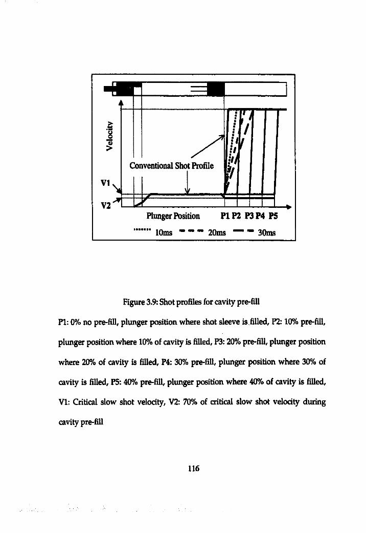
îV I

V2'

Conventional Shot Profile

gPlunger Position P1P2 P3P4 PS

" 10ms - - - 20ms — " 30ms

Figure 3.9: Shot profiles for cavity pre-fill

PI: 0% no pre-fill, plunger position where shot sleeve is filled, P2:10% pre-fill,

plunger position where 10% of cavity is filled, P3:20% pre-fill, plunger position

where 20% of cavity is filled, P4: 30% pre-fill, plunger position where 30% of

cavity is filled, P5:40% pre-fill, plunger position where 40% of cavity is filled,

VI: Critical slow shot velocity, V2: 70% of critical slow shot velocity during

cavity pre-fill

116

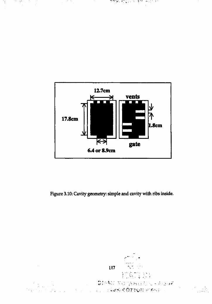
f-; , ' - î -

12.7cmvents

17.8cm1.8cm

6.4 or 8.9cm

Figure 3.10: Cavity geometry: simple and cavity with ribs inside.

117

■ ( F

Results

1. Effects of pre-fill percentage

Figure 3.11 shows the sequence of cavity filling in the simple cavity

geometry with narrow gate width (6.4cm) when transition time of 10ms is

employed. The simulations clearly showed that fill pattern is influenced by

cavity pre-fill. Specifically, more lateral expansion of flow in cavity was

observed when cavity pre-fill was used, which is desirable in terms of air

entrapment in this particular geometry of cavity since flow is injected more

before vents are sealed (blocked) with molten metal. However, high percentage

of cavity pre-fill (e.g. 40%) delayed fast shot engagement, so that lateral

expansion of flow was not fully promoted before the vents were sealed, hi this

particular geometry and selected transition time (10ms), 10,20, and 30% of cavity

pre-fills generate much better filling pattern in terms of air entrapment compared

to the injection without using cavity pre-fill. 30% of cavity pre-fill produced the

least air entrapment by generating more lateral expansion of flow before vents

were closed (Figure 3.11). Unlike using the narrow gate (6.4cm), in simple cavity

with wide gate (8.9cm), cavity pre-fill effects on the amount of air entrapment

were not as pronounced (Figure 3.14 A , 3.14.B).

In the die cavi^ with ribs inside wifli wide gate (8.9cm) and 10ms of

transition time (Figure 3.12), it was observed that the more pre-fill percentage

118

was used, the better fill patterns in terms of air entrapment were achieved.

Relatively low inertia of flow during pre-fill and lateral expansion of flow by fast

shot engagement right after pre-fill generated relatively uniform cavity fill. b\ the

predictable defect area, the gap between two ribs at the bottom were found to be

improved in terms of filling due to lateral expansion of the flow when cavity pre­

fill was used. Like simple geometry cavity fill, pre-fill effects on air entrapment

in the die cavity were larger with narrow gate width than with wide gate width.

2. Effects of transition time from slow to fast shot.

In addition to pre-fill percentage, the transition time firom slow to fast shot

on cavity filling patterns was found to be ah iihportant factor influencing cavity

f i l l i n g patterns. When cavity pre-fill was nob employed, the flow front of jet

stream was observed to be changed as transition time changed. The longer

transition time was used, the wider flow firont was generated. With cavity pre­

fill, transition time from slow to fast shot determined how early lateral expansion

of flow would be promoted. Since the pre-filled flow was pushed up by the

incoming fast flow without changes of flow firont, long transition time with high

pre-fill percentage delayed flow expansion and vents were closed even before

flow was expanded enough (Figure 3.13). Therefore, appropriate combinations

of transition time and pre-fill percentage should be used to achieve the best

performance to minimize air entrapment. For example, in Figure 3.14.B, while

119

10ms and 30% prefill shows best performance in terms of air entrapment, 20%

prefill was the best when 20ms of transition time was employed. Overall, 10ms

of transition time turned out to be desirable to minimize air entrapment in both

simple and cavity with ribs (Figure 3.14).

3. Effects of cavity geometry

Along with cavity prefill percentage and transition time, cavity geometry

including the areas and locations of gates and vents was found to be very

important factor, which should be considered to achieve optimum cavity fill in

terms of air entrapment. For the geometry of simple cavity in Figure 3.13,40% of

cavity prefill volume seemed to be too high percentage of cavity prefill with

30ms of transition time. In this case, it took only about 7ms after prefill for all

the vents to be closed with molten metal flow (i.e. about 23 more milliseconds

were still needed to reach fast shot velocity).

The effect of gate width on air entrapment in the die cavity was clear as can

be seen in Figure 3.14. Using wider gate, better performance in terms of air

entrapment was achieved than using narrower gate. On the other hand, cavity

pre-fill hardly helped reduce air entrapment when wider gate was used, while

the cavity pre-fill significantly influenced the amount of trapped air when

narrower gate was used.

120

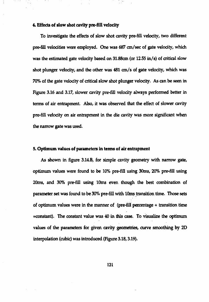
4. Effects of slow shot cavity pre-fill velocity

To investigate the effects of slow shot cavity pre-fill velocity, two different

pre-fill velocities were employed. One was 687 cm/sec of gate velocity, which

was the estimated gate velocity based on 31.88cm (or 12.55 in/s) of critical slow

shot plunger velocity, and the other was 481 cm/s of gate velocity, which was

70% of the gate velocity of critical slow shot plunger velocity. As can be seen in

Figure 3.16 and 3.17, slower cavity pre-fill velocity always performed better in

terms of air entrapment. Also, it was observed that the effect of slower cavity

pre-fill velocity on air entrapment in the die cavity was more significant when

the narrow gate was used.

5. Optimum values of parameters in terms of air entrapment

As shown in figure 3.14.B, for simple cavity geometry with narrow gate,

optimum values were found to be 10% pre-fill using 30ms, 20% pre-fill using

20ms, and 30% pre-fill using 10ms even though the best combination of

parameter set was found to be 30% pre-fill with 10ms transition time. Those sets

of optimum values were in the manner of (pre-fill percentage + transition time

=constant). The constant value was 40 in this case. To visualize the optimum

values of the parameters for given cavity geometries, curve smoothing by 2D

interpolation (cubic) was introduced (Figure 3.18,3.19).

121

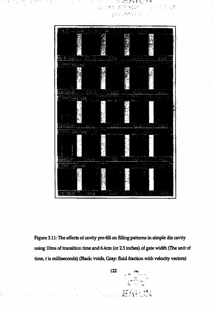
Figure 3.11: The effects of cavity prefill on filling patterns in simple die cavity

using 10ms of transition time and 6.4cm (or 2.5 inches) of gate width (The unit of

time, t is milliseconds) (Black: voids. Gray: fluid firaction with velocity vectors)

122

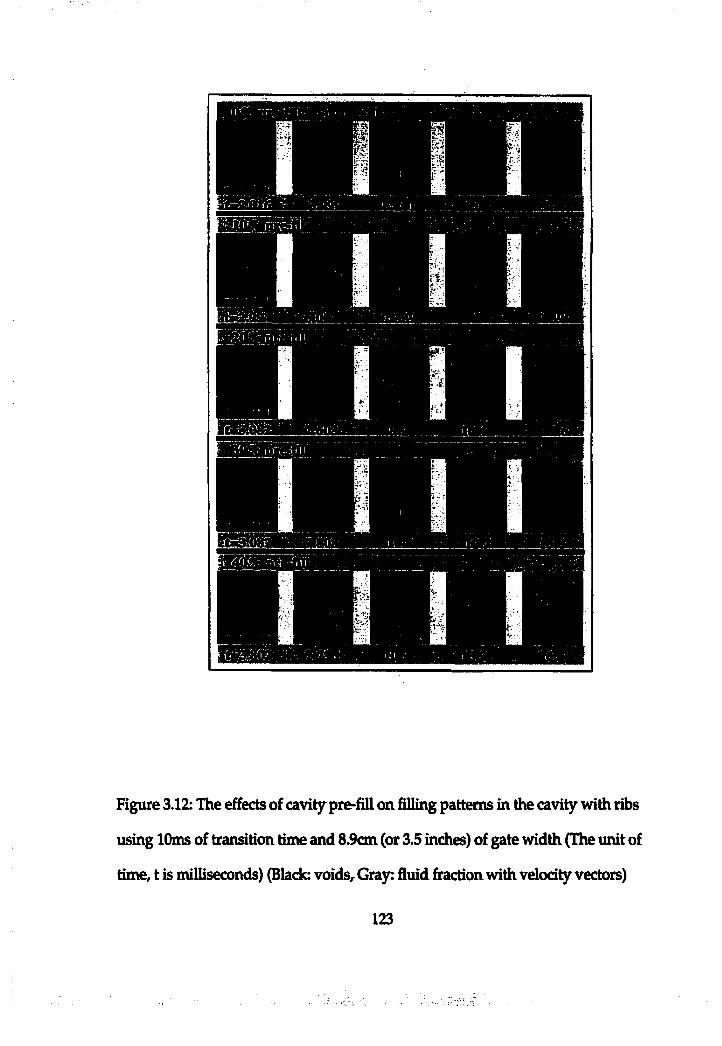
Figure 3.12: The effects of cavi^ pre-fill on filling patterns in the cavity with ribs

using 10ms of transition time and 8.9cm (or 3.5 inches) of gate width (The unit of

time, t is milliseconds) (Black: voids. Gray: fluid fraction with velocity vectors)

123

Figure 3.13: The eâiects of transition time on filling patterns in simple die cavity

using 40% of cavity pre-fill and 6.4cm (or 2.5") of gate width (Black: voids. Gray:

fluid firaction with velocity vectors)

124

AlrBMnpmmt ( Simplt cmity & Wld» gMt wldHi )

10% aOK 30% 40%Mromiigi CMttif n»4ll

(%oromtyvolunM)

lOnns -» aome •aorm

AirBtfnipmmt ( Slmpl* cmiljf AMmowgMi widih )

40%MroMilag* CMRy nr»4l

(%olem#y*olum#)10ms •» . 20ms •30ms

B

Figure 3.14: The estimated amount of air traipped in the die cavity A: Simple

cavity with wide gate w idth, 8.9 cm (or 3.5")/ Br Simple cavity with narrow

gate w idth, 6.4cm (or 2.5")

125

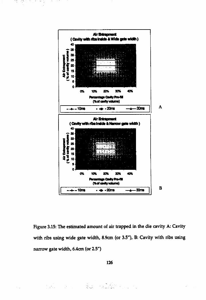
AirBttipmmt (GkvNy «vflh riteiraidt ft WMi grti wktti )

10% 20%

hreintaoi CMity (%arcMRyvolunM)

— # — lOlhtt • 20ms 30mg

Î

hraMNiBi CMty(%cfawtly¥olum>)

•» -aonm -30m B

Figure 3.15: The estimated am ount of air trapped in the die cavity A: Cavity

with ribs using wide gate w idth, 8.9cm (or 3.5"), B: Cavity w ith ribs using

narrow gate w idth, 6.4cm (or 2.5")

126

Ak w l IVo DMmM n » 4 i VML(ShpkCNÊy&WMkCM#**##

Peeetigi Qe*vn»fli (KcTonMifwiumi)

-687cnY s - a - 481 cm&

Air IV» OflÉat nifll VW.(SIniteCMyAHBrewGMiVMdti)

0% 10% 20% 30%

(%acm#yvoiimn#

40%

-687cm^ I- 481cmAs B

Figure 3.16: The effect of prefill velocity (10ms of fixed transition time). A:

Simple cavity with wide gate width, 8.9cm (or 3.5"), B: Simple cavity with

narrow gate width, 6.4cm (or 2.5")

127

':'3'

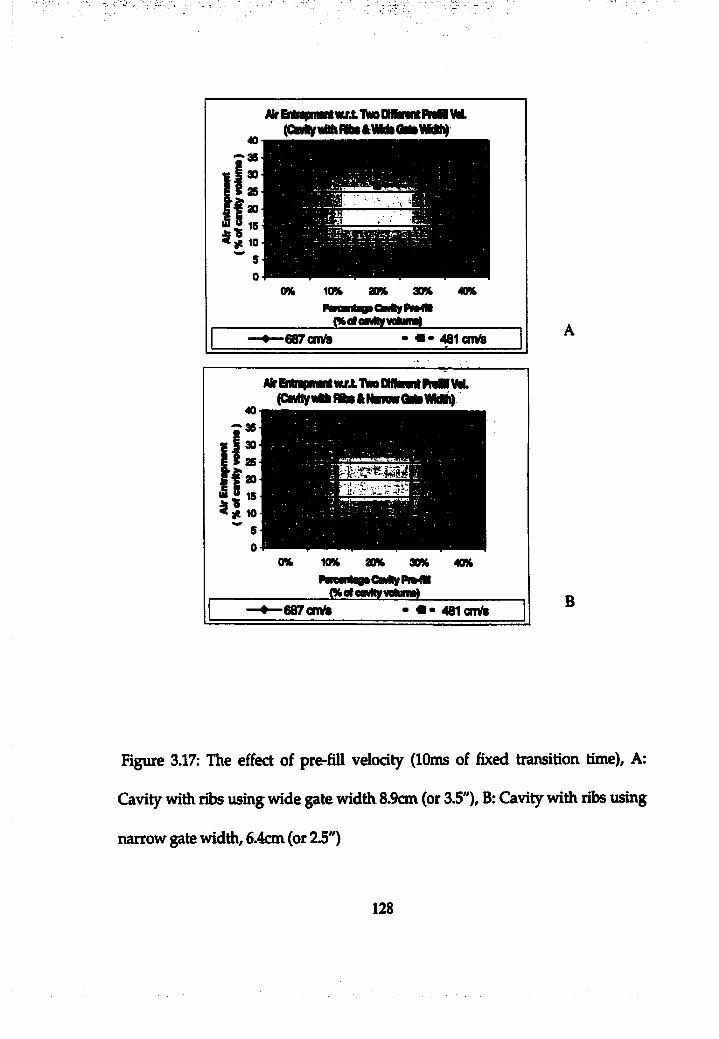
f10% aoK 30%FewnbgiQweyPiwie

(%«*e*#ywlum#-687cnV!B 481 cm^

AkBiln4Ni« 4%iw±TWoDlllMnllWNVil(Gn%iiMinbiâNnawGrii¥IMi4

f10% 30% 30%N w 4igiCl 3yft»Wi

(%of«Mllywlum»)

40K

687cm% 481cm/lBB

Figure 3.17: The effect of pre-fill velocity (10ms of fixed transition time). A:

Cavity with ribs using wide gate width 8.9cm (or 3.5")» B: Cavity with ribs using

narrow gate width, 6.4cm (or 2.5")

128

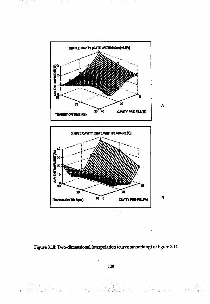
SIMPLE CAV nY[GA TEW ID TH :8.9ein(-a.8^]

TRANSmONTIMEdm) 30 40 CAVITY PRE>FIIK%)

SIMPLE CAVITY [QATEWHrnt0.4«m("2.y)|

TRANSmONTIMEtm) 10 0 CAVITY PRGflLK*) B

Figure 3.18: Two-dimensional interpolation (curve smoothing) of figure 3.14

129

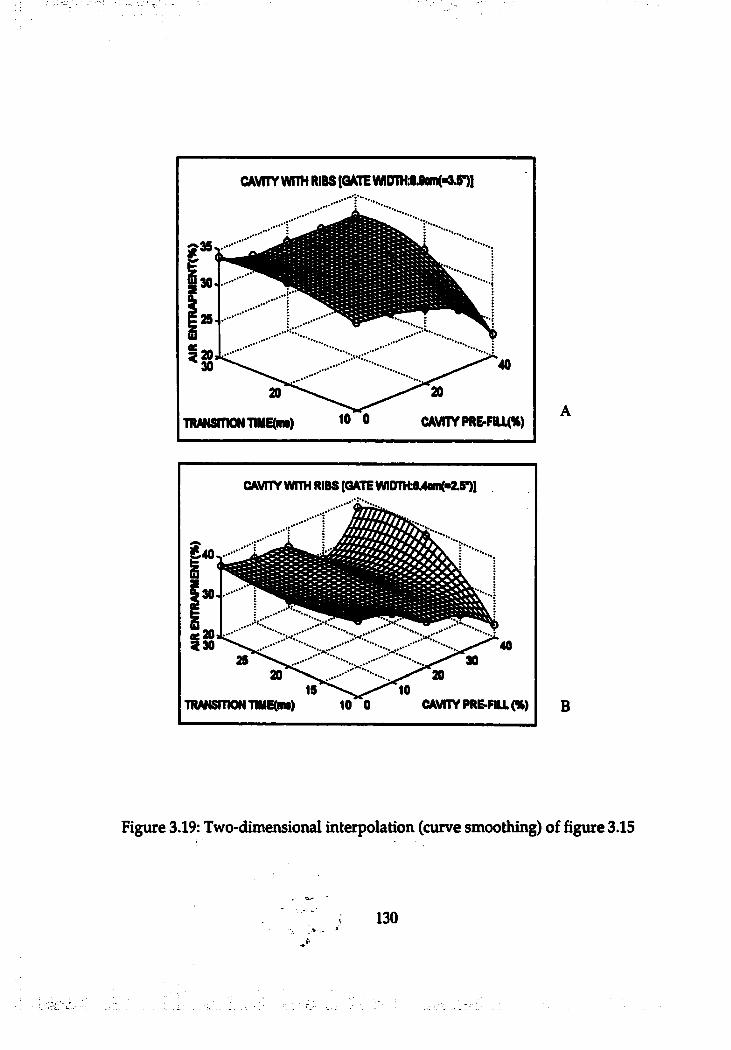
CAVITY W nH RIBS [GATE VM0mMJem(>9.5*)l

TRANSITION T1ME(m») 10 0 CAVITY PR&FILM%)

CAVMYWrm RIBS [Q A T E W I0riH :6^ -2 .S ^ l

TRANSITION TIMGdm) 10 0 CAVITY PRE-FILL (« ) B

Figure 3.19: Two-dimensional interpolation (curve smoothing) of figure 3.15

130

3.2 Three dimensional computer flow model

Using three dimensional die cavities, three-dimensional computer flow

models were developed to visualize and investigate three-dimensional

cavity fill patterns when using cavity pre-fill. The three dimensional testI

cavity geometries were similar to two dimensional cavity geometries in

Chapter 3.1.

3.2.1 Modeling

In three-dimensional modeling, assumptions were basically the same as

made in two-dimensional modeling except cavity geometry, critical slow

shot velocity, and fast shot velocity.

Critical slow shot plunger velocity was assumed to be 14.3 in/sec (36.32

cm/sec), which was obtained based on 55% of initial fill in the shot sleeve,

2.0 in (5.08 cm) of sleeve inner diameter, 19.94 in (50.65 cm) of sleeve length,

and 2.1 in /sec /in of acceleration rate from slow to fast shot using Thome's

calculator. 1500 in/sec (3810 cm/sec) of fast shot gate velocity was used.

Cavity geometries were basically the same as used in two-dimensional

models, but have 0.5 inch thickness. To visualize effects of flow gating

directions when usiiig cavity pre-fill, two different types of gates were

employed in addition to two difrerent gate widths (Figure 3.20). One was fan

gate type and the other one was chisel gate. Therefore, unlike two-

131

dimensional flow models, three-dimensional models included runners and

gates.

132

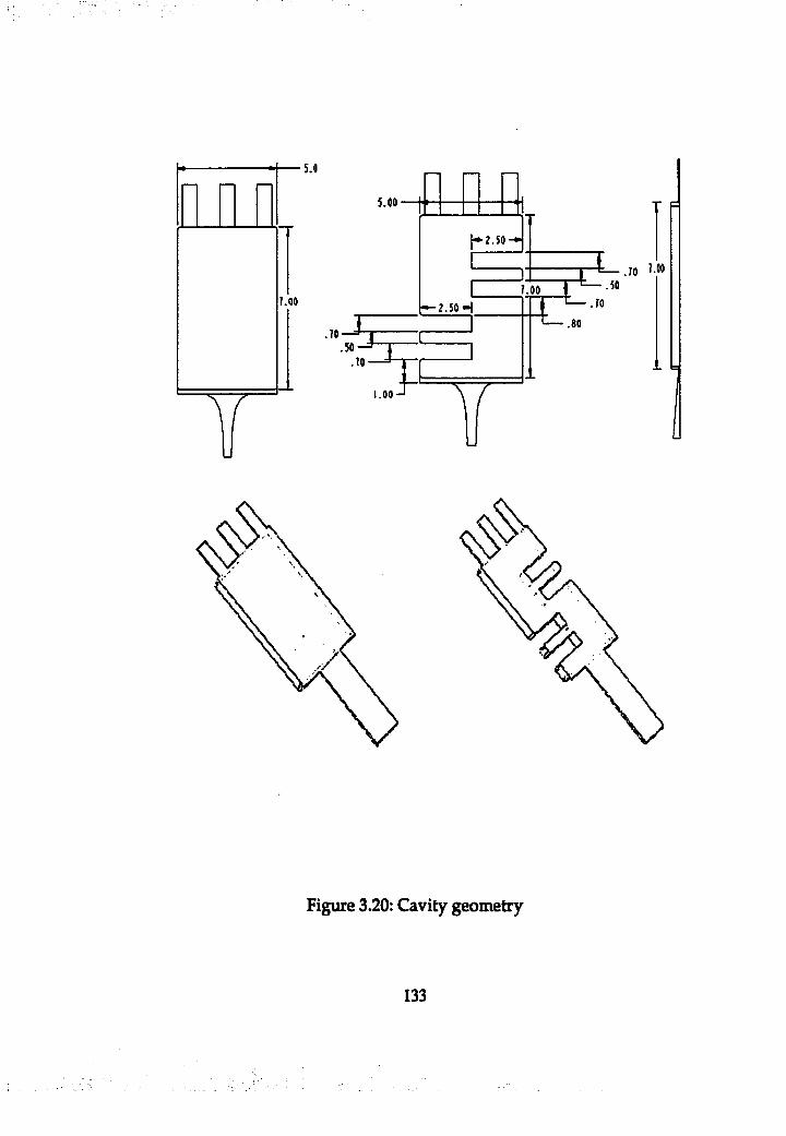
?.oo

5.0

5.00-

.10J.50

1 * 2 .5 0 —

— 2 .5 0 H

.10

1.00 Î T

. 0 0 * • T T t _ . i n

t — an

T -Ï—.10t — 50

Figure 3.20: Cavity geometry

133

3.2.2 Pre-fill effects on flow pattern

Unilateral expansion of flow in both x and y directions was observed in three

dimensional computer models of cavity pre-fill (Figure 3.21), while two

dimensional lateral expansion was found in two dimensional computer flow

models. Figure 3.21 shows a sequence of flow pattern in the simple rectangular

die cavity when cavity pre-fill is employed with 55 ms transition time, 10%

cavity pre-fill, and 40% of critical slow shot gate velocity (i.e. 312.6 cm/sec) as a

cavity pre-fill velocity. The circled areas are the areas where flow is expanded

unilaterally. The degree of the unilateral expansion varied using different cavity

pre-fill slow velocity, transition time, and amount of cavity pre-fill as observed in

two dimensional computer flow model.

134

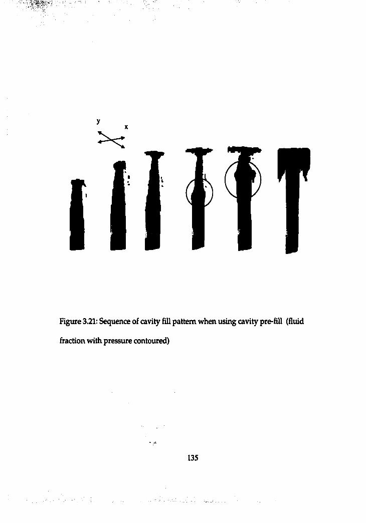
T

Figure 3.21: Sequence of cavity fill pattern when using cavity pre-fill (fluid

fraction with pressure contoured)

135

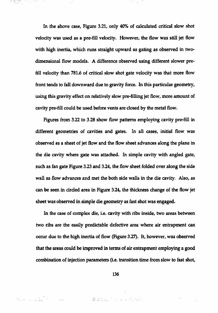
In the above case. Figure 3.21, only 40% of calculated critical slow shot

velocity was used as a pre-fill velocity. However, the flow was still jet flow

with high inertia, which runs straight upward as gating as observed in two-

dimensional flow models. A difference observed using different slower pre­

fill velocity than 781.6 of critical slow shot gate velocity was that more flow

firont tends to fall downward due to gravity force. In this particular geometry,

using this gravity effect on relatively slow pre-filling jet flow, more amount of

cavity pre-fill could be used before vents are closed by the metal flow.

Figures fiom 3.22 to 3.28 show flow patterns employing cavity pre-fill in

different geometries of cavities and gates. In all cases, initial flow was

observed as a sheet of jet flow and the flow sheet advances along the plane in

the die cavity where gate was attached. In simple cavity with angled gate,

such as fan gate Figure 3.23 and 3.24, the flow sheet folded over along the side

wall as flow advances and met the both side walls in the die cavity. Also, as

can be seen in circled area in Figure 3.24, the thickness change of the flow jet

sheet was observed in simple die geometry as fast shot was engaged.

In the case of complex die, i.e. cavity with ribs inside, two areas between

two ribs are the easily predictable defective area where air entrapment can

occur due to the high inertia of flow (Figure 3.27). It, however, was observed

that the areas could be improved in terms of air entrapment employing a good

combination of injection parameters (i.e. transition time from slow to fast shot,

136

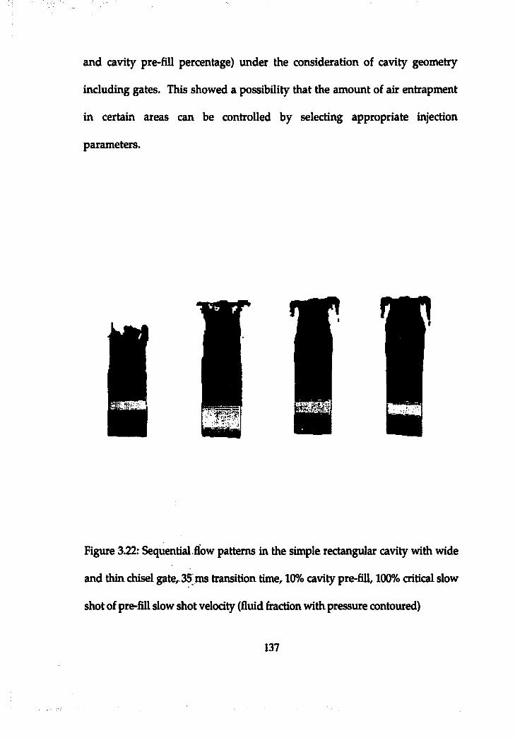
and cavity pre-fill percentage) under the consideration of cavity geometry

including gates. This showed a possibility that the amount of air entrapment

in certain areas can be controlled by selecting appropriate injection

parameters.

Figure 3.22: Sequential flow patterns in the simple rectangular cavity with wide

and thin chisel gate, 35 ms transition time, 10% cavity pre-fill, 100% critical slow

shot of pre-fill slow shot velocity (fluid firaction with pressure contoured)

137

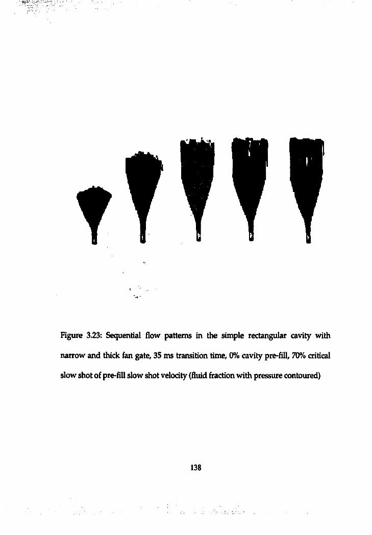
tTTT!Figure 3.23: Sequential flow patterns in the simple rectangular cavity with

narrow and thick fan gate, 35 ms transition time, 0% cavity pre-fill, 70% critical

slow shot of pre-fill slow shot velocity (fluid firaction with pressure contoured)

138

i J

Figure 3.24: Sequential flow patterns in the simple rectangular cavity with wide

and thin fan gate, 55 ms transition time, 10% cavity pre-fill, 40% critical slow shot

of pre-fill slow shot velocity (fluid fraction with pressure contoured)

139

Figure 3 ^ : Sequential flow patterns in the ribbed cavity with wide and thin fan

gate, 35 ms transition time, 30% cavity pre-flll, 40% critical slow shot of pre-fill

slow shot velocity (fluid fraction with pressure contoured)

140

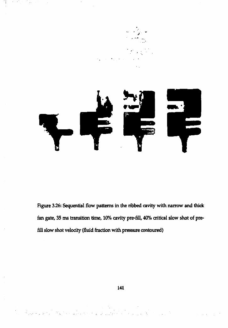
Figure 3.26: Sequential flow patterns in the ribbed cavity with narrow and thick

fan gate, 35 ms transition time, 10% cavity pre-fill, 40% critical slow shot of pre­

fill slow shot velocity (fluid fraction with pressure contoured)

141

Figure 3.27: Sequential flow patterns in the ribbed cavity with narrow and thick

chisel gate, 65 ms transition time, 20% cavity pre-fill, 70% critical slow shot of

pre-fill slow shot velocity (fluid firaction with pressure contoured)

142

Figure 3.28: Sequential flow patterns in the ribbed cavity with wide and thin

chisel gate, 55 ms transition time, 10% cavity pre-fill, 100% critical slow shot of

pre-fill slow shot velocity (fluid firaction with pressure contoured)

143

3.2.3 Gravity effect in cavity pre-fill

When gates were at the bottom of cavities and relatively low gate velocity

(low inertia of flow) as compared to gravity force (e.g. 50 cm/sec) was used, it

was observed that gravity helped reduce inertia of flow and develop more

uniform cavity flow as flow expanded (Figure 2.25). As relatively low gate

velocity is used during cavity pre-fill stage in cavity pre-fill approach, the

above beneficial gravity effect employing cavity pre-fill approach was

investigated using computer flow models.

As a result, unfortunately, it was observed that gravity effect on flow

patterns during pre-fill stage was insignificant since the inertia of the flow

was still very high as compared to gravity force. In cavity pre-fill approach,

the beneficial flow expansion was caused mainly by collision between two

different inertia of flow, slow pre-fill flow and fast shot flow (Figure 3.29).

For the above reason, even when gates were located at the side of cavities,

the flow expansion was observed using cavity pre-fill, while the smooth

change of flow direction during cavity pre-fill was observed (Figure 3.29.C).

In other words, considering cavity geometry including locations of gates and

vents, cavity pre-fill approach is still helpful to reduce air entrapment as

cavity flow expands even when side gates are used. However, using high

percentage of cavity pre-fill with side gates can cause unwanted side effects,

such as flow lines in the castings.

144

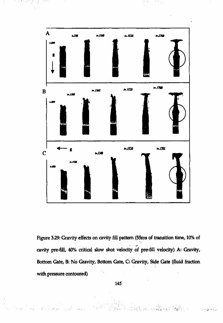
t~J7W

M700imjmtrn.im

ItmJ520

Figure 3.29: Gravity effects on cavity fill pattern (55ms of transition time, 10% of

cavity pre-fill, 40% critical slow shot velocity of pre-fill velocity) A: Gravity,

Bottom Gate, B: No Gravity, Bottom Gate, C: Gravity, Side Gate (fluid firaction

with pressure contoured)

145

3.3 Evaluation of quantitative estimation

As shown earlier in chapter 3.1 a method of quantitative estimation was

developed to measure performances of cavity pre-fill in terms of amount of air

entrapment in the die cavity using computer flow models. The estimation

was evaluated by comparing with available experimental results [Brevick, 94].

3.3.1 Estimation of amount of air entrapment

Under the assumption that vents are the only way out for air in the die

cavity to escape out of the die cavity, air inside the die cavity should be

trapped in the die cavity as soon as all the vents are closed with molten alloy.

Using the above assumption, the procedure of estimation method was as

follows: 1) measure the time when vents are sealed in computer flow

simulation, 2) calculate the amount of flow in volume based on known flow

rate (or shot profile) and time measured, 3) calculate the amount of unfilled

cavity volume when vents are all sealed based on known total cavity volume

and calculated volume of molten metal gated in by the time when vents are all

closed. The volume calculated in the step 3 will be the amount of air

entrapment in the die cavity.

As an example, a Pac-Man casting f ig u re 3.30) was simulated using

Flow3D since its experimental results were available [Brevick, 94]. To

compare the results of experimental casting, the same cavity geometry and

146

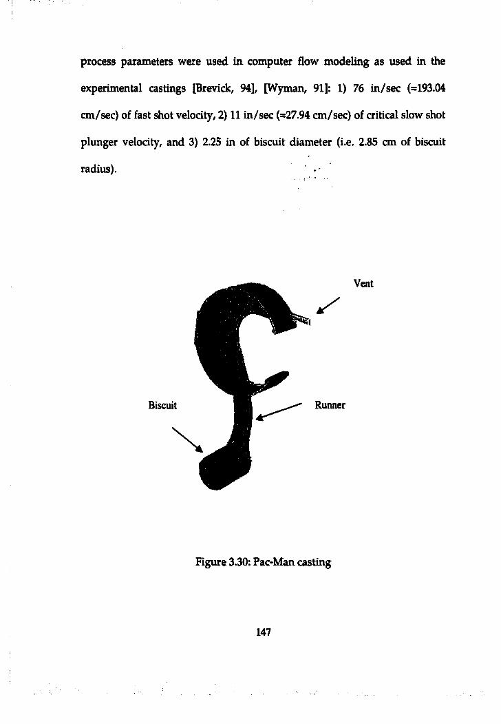
process parameters were used in computer flow modeling as used in the

experimental castings [Brevick, 94], [Wyman, 91]: 1) 76 in/sec (=193.04

cm/sec) of fast shot velocity, 2) 11 in/sec (=27.94 cm/sec) of critical slow shot

plunger velocity, and 3) 2.25 in of biscuit diameter (i.e. 2.85 cm of biscuit

radius). ‘ +

Biscuit

Vent

Runner

Figure 3.30: Pac-Man casting

147

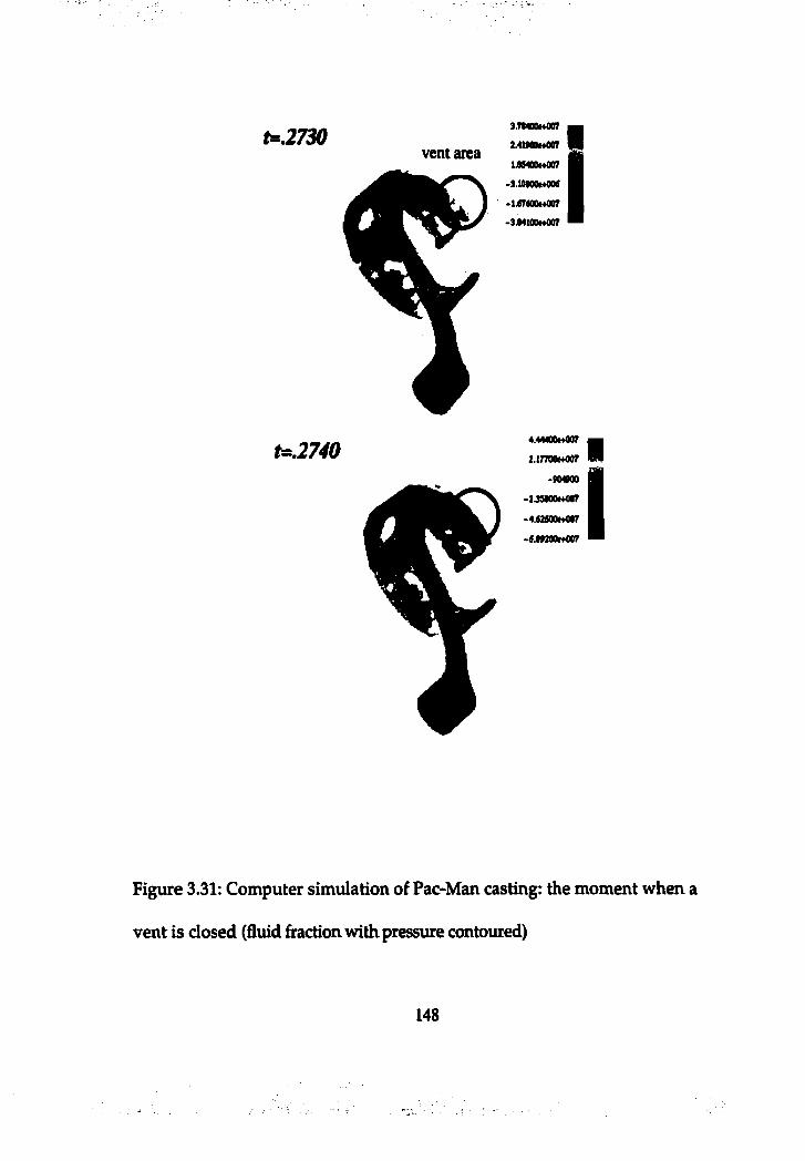
t= .2730vent area

-3 .U «0m 0M

•liTwiowm

t^ .2 7 4 04*MOOwOOTl.lTTOOwW

-M M O O

- I J S M O h OOT

-4.62M0H«tr

Figure 3.31: Computer simulation of Pac-Man casting: the moment when a

vent is closed (fluid firaction with pressure contoured)

1 4 8

Using the above process parameters^ dimensions, and 2.72 g/cc of theoretical

density of A1390, simulation was conducted, fig u re 3.31). As can be seen in

Figure 3.31, a vent was closed between 0.2731 sec and 0.2740 sec (the time

0.2731 or 0.2740 sec is not a cavity fill time only. The time includes biscuit

and runner fill time as modeled). Therefore, volume filled by the time when

a vent was closed was calculated based on known shot profile and

dimensions of cavity geometry including runners and biscuit (i.e. flow rate)

(Table 3.1).

Table 3.1 shows 10 possible estimated volume amount of gas entrapment in

the die cavity since it was not clear when exactly a vent was sealed with molten

alloy between time 0.2739 and 0.2740 second. As can be seen in the table, 0.1

milliseconds made a relatively meaningful difference in gas content of cc/lOOg.

The result plots (Figure 3.31) of simulation were generated every 1 millisecond as

programmed.

The 'volume of trapped air' in Table 3.1 was estimated based on the

estimated volume filled by the time when vents were closed and total

volume including biscuit and runner (i.e. 326.80 cc) estimated using CAD

data. Also, the volume of trapped air in % of cavity volume (i.e. 157.42 cc)

was calculated and shown in the table.

The amount of 'contained gas content' was obtained using the cavity

volume (i.e. 157.42 cm^), theoretical value of density of A1390 (i.e. 2.72 g/cc),

149

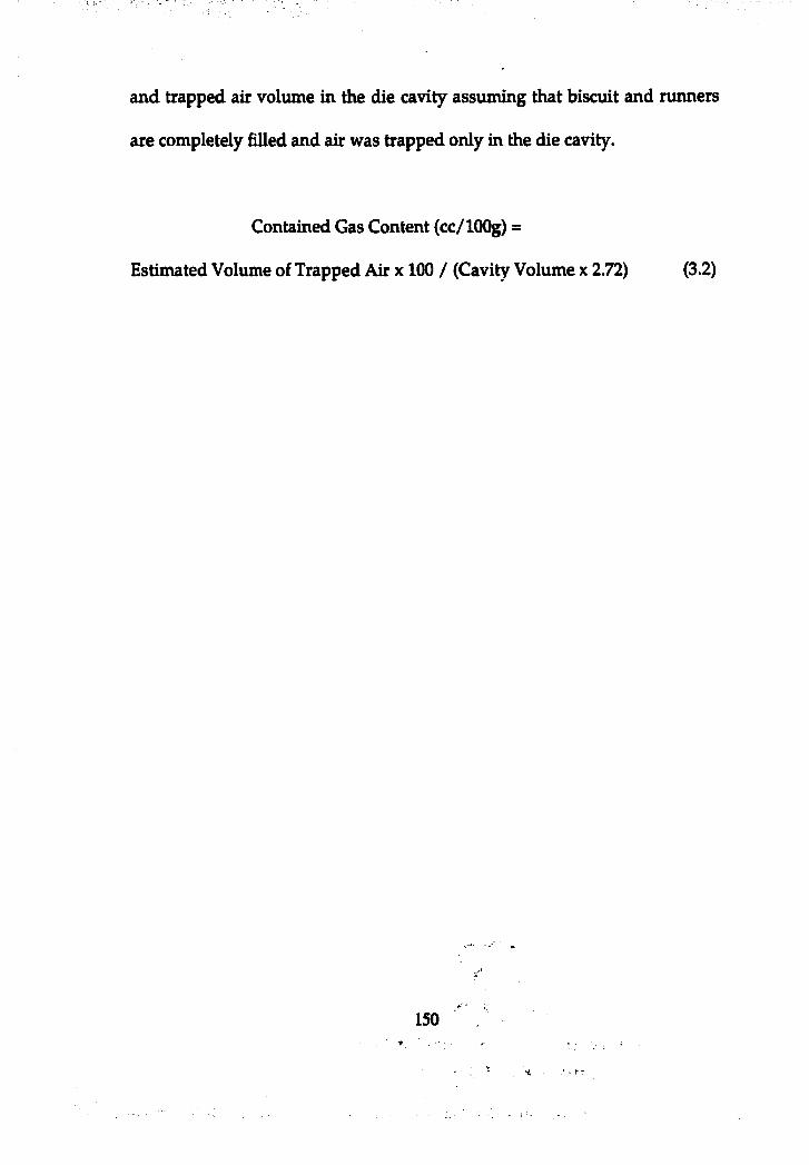
and trapped air volume in the die cavity assuming that biscuit and runners

are completely filled and air was trapped only in the die cavity.

Contained Gas Content (cc/lOOg) =

Estimated Volume of Trapped Air x 100 / (Cavity Volume x 2.72) (3.2)

150

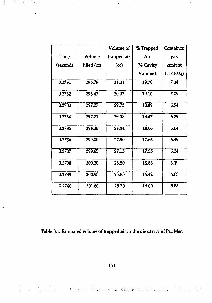
Time

(second)

Volume

filled (cc)

Volume of

trapped air

(cc)

% Trapped

Air

(% Cavity

Volume)

Contained

gas

content

(cc/lOOg)

0.2731 295.79 31.01 19.70 7.24

0.2732 296.43 30.07 19.10 7.09

0.2733 297.07 29.73 18.89 6.94

0.2734 297.71 29.08 18.47 6.79

0.2735 298.36 28.44 18.06 6.64

0.2736 299.00 27.80 17.66 6.49

0.2737 299.65 27.15 17.25 6.34

0.2738 300.30 26.50 16.83 6.19

0.2739 300.95 25.85 16.42 6.03

0.2740 301.60 25.20 16.00 5.88

Table 3.1: Estimated volume of trapped air in the die cavity of Pac Man

151

3.3.2 Evaluation of estimation

Contained gas content in experimental castings made was measured using

vacuum fusion test. The vacuum fusion test, described schematically in Figure

3.32, consists of placing the casting in the crucible and then sealing it in a bell jar.

The bell jar is then vacated and isolated hom the vacuum pump by closing the 3-

way valve. After the level of vacuum is recorded from the manometer, the

casting is heated to its melting point using the induction furnace. Gas contained

in the casting is released as the casting melts and the pressure rise in the bell jar

is indicated by the manometer. The pressure rise is then used to calculate the

amount of gas that was contained in the casting in units of cc gas per 100 grams

of aluminum at standard temperature and pressure. The method of calculation

is shown in the Appendix A [Brevick, 94].

The vacuum fusion test is a more appropriate method for assessing air

entrapment in the die cavity than is Archimedes test. When shrinkage voids are

created in the castings during solidification, the Archimedes density of castings

would include the shrinkage voids, in which no air or a very little amount of air

is. The developed estimation of air entrapment using computer models is the

amount of air trapped in the die cavity at standard temperature and pressure. It

is not associated with shrinkage voids.

The measured average value obtained from the experiment was 6.3 cc/lOOg,

which is in the range of the above estimate, from 7.24 to 5.88 cc/lOOg. Also, the

152

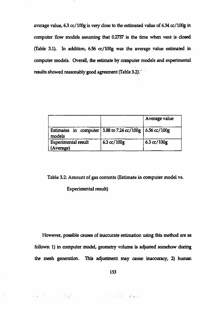
average value, 6.3 cc/lOOg is very dose to the estimated value of 6.34 cc/lOOg in

computer flow models assuming that 0.2737 is the time when vent is dosed

(Table 3.1). hi addition, 6.56 cc/lOOg was the average value estimated in

computer models. Overall, the estimate by computer models and experimental

results showed reasonably good agreement (Table 3.2)".'

Average value

Estimates in computer models

5.88 to 7.24 cc/lOOg 6.56 cc/lOOg

Experimental result (Average)

6.3cc/100g 6.3cc/100g

Table 3.2: Amount of gas contents (Estimate in computer model vs.

Experimental result)

However, possible causes of inaccurate estimation using this method are as

follows: 1) in computer model, geometry volume is adjusted somehow during

the mesh generation. This adjustment may cause inaccuracy, 2) human

153

judgment of time when vents are closed may cause inaccurate results, 3) ignoring

air entrapment in the shot sleeve may also cause inaccuracy.

154

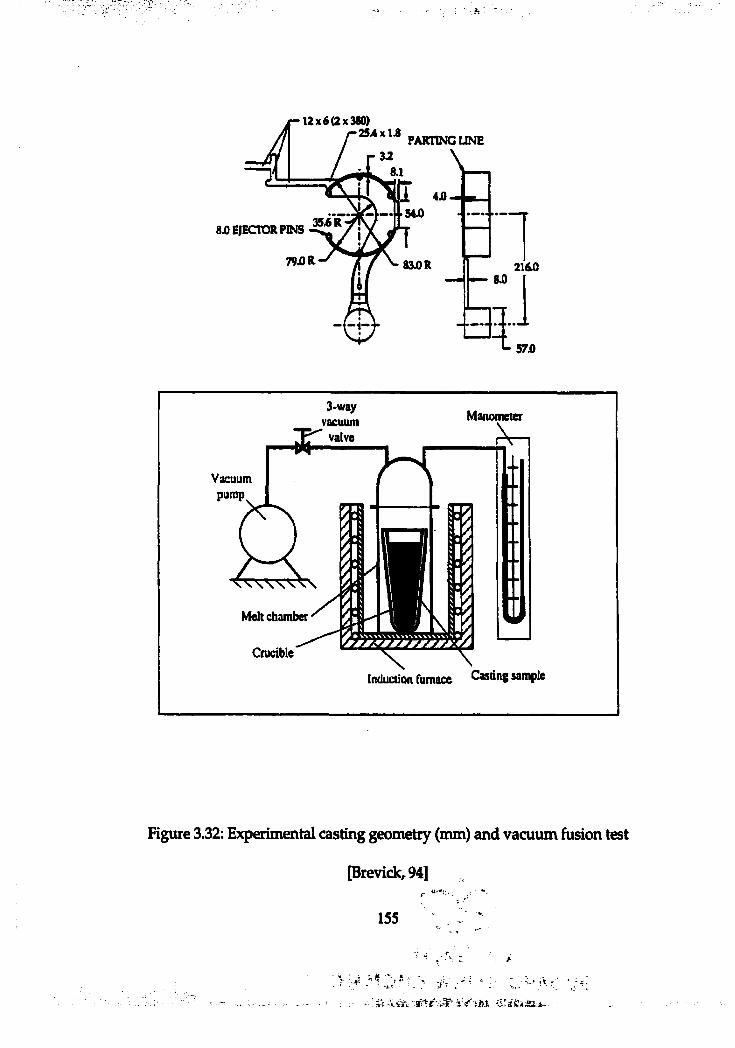
12x6(2x380)PARTING UNE

8i)E)ECrORPIN5

S7Û

Vacuumpump

r - s :

3-wayvacuum

valve

Melt chamber

Crucible

Manometer

Induction furnace Casting sample

Figure 3.32: Experimental casting geometry (mm) and vacuum fusion test

[Brevick, 94]r ■ ' ■

155 ‘

CHAPTER4

WATER MODELING

As a physical model approach, water analog testing was conducted for

qualitative evaluation of computer flow models using Flow3D. For the

evaluation, three different geometries of cavities including gates and runners

were selected, designed, and fabricated using thick acrylic blocks for the

transparency. Water analog experiments on the test stand were recorded

using a high-speed video camera.

4.1 Die cavity design

Three different die geometries were designed for water analog testing:

simple, intermediate, and complex. Among the three, the simple and

intermediate complexity cavity geometries were the same as those used in

the computer flow models. For the high complexity die geometry, an

Adapter Plate was selected.

156

A rectangular plate die was selected as the simple complexity die

geometry (Figure 4.1). The intermediate complexity geometry was designed

to investigate the flow behavior of rapid flow direction changes after

impingement on the obstacles in the die cavity. Also, the possibility of air

entrapment was intentionally designed into the intermediate complexity die

by attaching four ribs into the simple die cavity (Figure 4.2).

Water analog simulation was limited to two-dimensional results due to

difficulties of fabrication of transparent die and lack of equipment for three-

dimensional image processing. For that reason, a relatively two-dimensional

cavity geometry (Figure 4.3), which is called Adapter Plate, was selected as

the high complexity cavity geometry. This cavity has thin and thick cross

sections with bosses and pockets that may complicate the flow during filling.

157

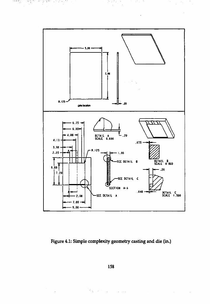
6.75

3.002.25

.1251.00

see D E T A I L

9.00

rSECTION A-A

SEC DETAIL A

7.009.00

.075

DETAIL B SCALE 0 800

.040

Figure 4.1: Simple complexity geometry casting and die (in.)

158

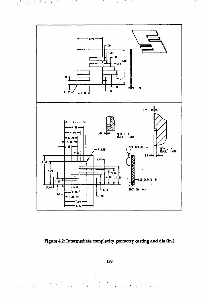
.11I.M

L-.W

.075

$ M

*.125

.20

1 2 tT *-‘® I

« w I, Î.IO1.10

2.40

4 .SI

7.000.00

Figure 4.2: Interm ediate complexity^ geometry casting and die (in.)

159

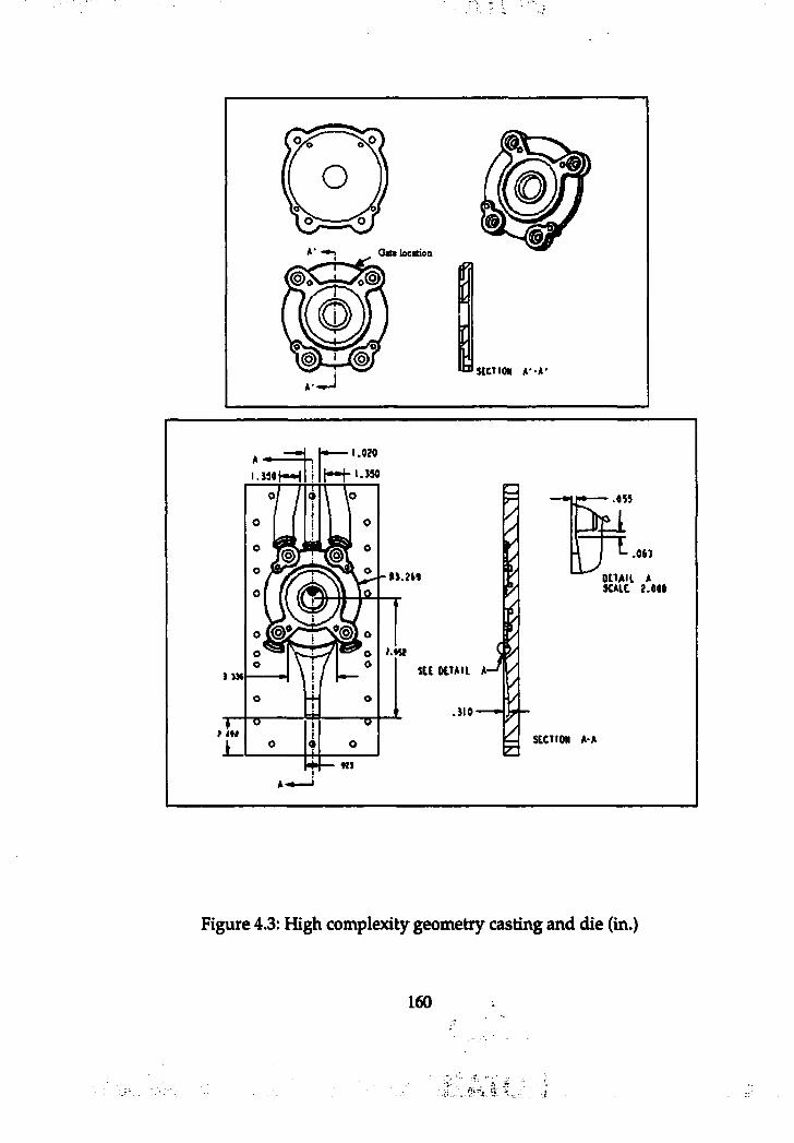
nGateloeatioa

O SUT ion * '•* '

.O il

OlUll * SCALC 2.04»

4-310

f été

A

Figure 4.3: High complexity geometry casting and die (in.)

160

4.2 Gate and runner design

The gate area was designed using the following procedure: 1) calculate

required cavity fill time using equation 4.1, 2) calculate fill rate based on

cavity volume and required fill time, 3) determine gate velocity using

equation 4.2, 4) to calculate gate area based on fill rate and gate velocity

found. * "

Maximum allowable cavity fill time [Wallace, 68]:

0 .86«xTxCr,-T^+P)' '

where,

t = required cavity fill time (seconds)

T = minimum thickness (inches); 0.2 inches.

Tiiq = liquidus temperature for metal (F); for Aluminum A380 = 1095 F.

P = Percent Solid Factor (F); for 50% solid, P = 340 F.

Id = die cavity temperature (F); assumed to be 650 F (Brevick, 1999).

Minimum gate velocity, Russ Van Rens equation [Prince, 97]:

lOjmGv =

750W .xG,

(4.2)

where,

161

Gv = Kfinimum gate velocity for atomized flow

Wd = Weight density of metal=0.093 Ib/iii* (for aluminum)

Gt = gate thickness = 0.04 in (determined)

For the simple and intermediate complexity cavity geometries, following

results were obtained based on the above procedure and assumptions: 1) the

maximum allowable cavity fill time for simple die = 141 ms, 2) calculated fill rate

= 49.57 in^/sec, 3) required gate velocity = 1319 in/sec. Thus, calculated gate area

was 0.0376 in , which was obtained by fill rate divided by gate velocity. This is

the minimum gate area to meet the requirement of maximum cavity fill time. In

this experiment, a gate area of 3.65x0.04 in^ was used, which is larger than the

minimum gate area.

Runner area should be bigger than gate area to create a pressurized gating

system to avoid air entrapment in the runner during filling. Rao suggested ratio

of runner area to gate area (Rao, 1989) (Table 4.1) and the ratio of designed

runner for simple and intermediate complexity of die cavities was: 1) 0.99 of

runner are to gate area, 2) 1.72 of runner width to gate width, 3) 1.33 of fan

feed length to gate width (Figure 4.4).

162

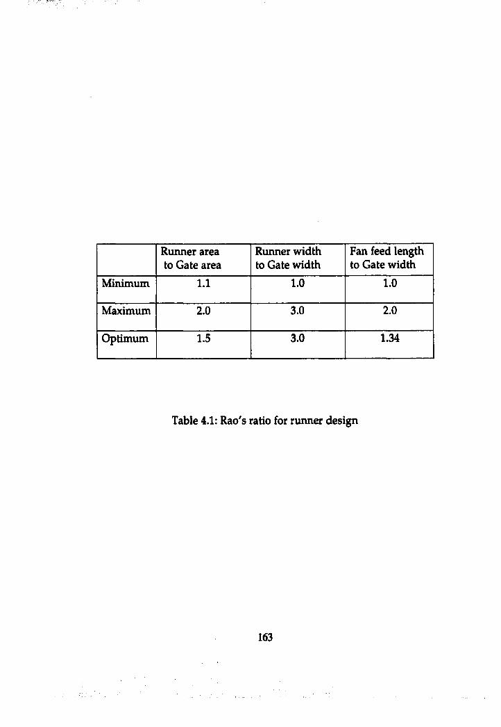
Runner area to Gate area

Runner width to Gate width

Fan feed length to Gate width

Minimum 1.1 1.0 1.0

Maximum 2.0 3.0 2.0

Optimum 1.5 3.0 1.34

Table 4.1: Rao's ratio for runner design

163

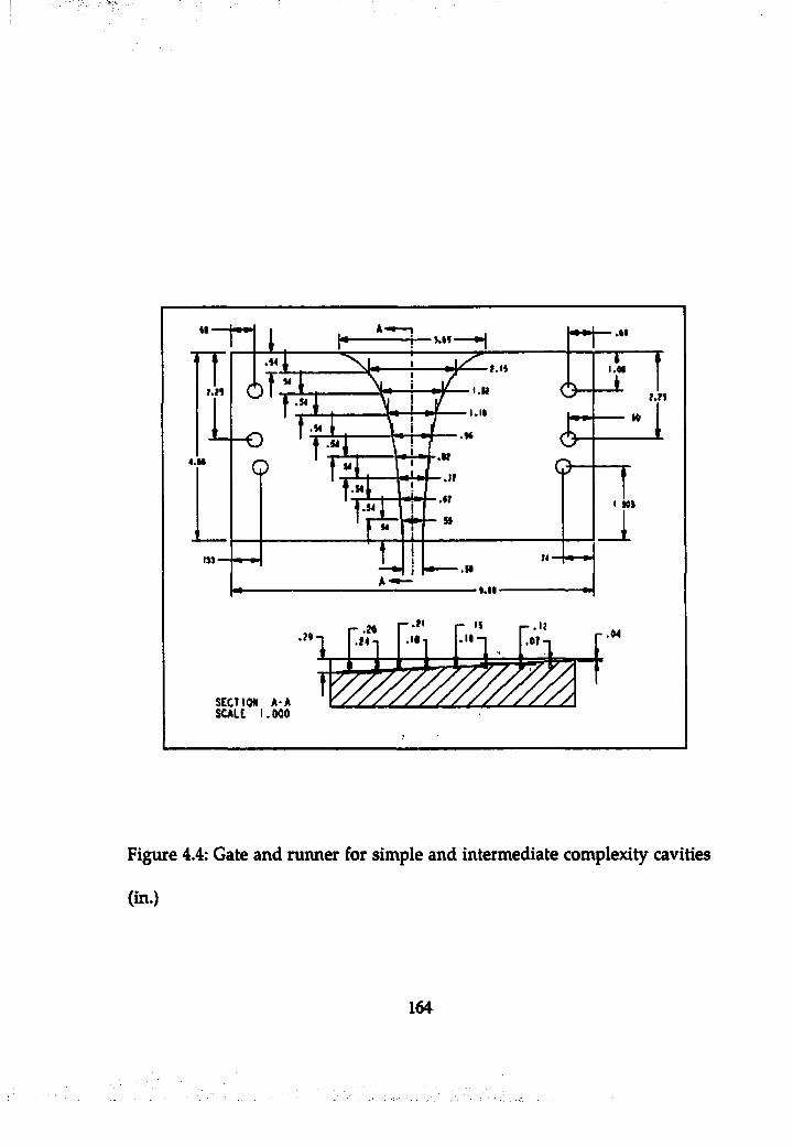
*1

I.MI.K

1. 1»

.WM4.U

I MS

tS] M

SECTION A-A SCALE 1.000

r M

Figure 4.4: Gate and runner for simple and intermediate complexity cavities

(in.)

164

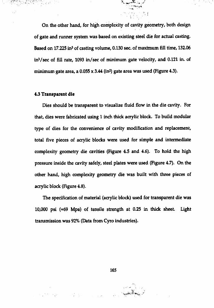
On the other hand, for high complexity of cavity geometry, both design

of gate and runner system was based on existing steel die for actual casting.

Based on 17.225 in^ of casting volume, 0.130 sec. of maximum hll time, 132.06

in^/sec of fill rate, 1093 in/sec of minimum gate velocity, and 0.121 in. of

minimum gate area, a 0.055 x 3.44 (in^) gate area was used (Figure 4.3).

4.3 Transparent die

Dies should be transparent to visualize fluid flow in the die cavity. For

that, dies were fabricated using 1 inch thick acrylic block. To build modular

type of dies for the convenience of cavity modification and replacement,

total five pieces of acrylic blocks were used for simple and intermediate

complexity geometry die cavities (Figure 4.5 and 4.6). To hold the high

pressure inside the cavity safely, steel plates were used (Figure 4.7). On the

other hand, high complexity geometry die was built with three pieces of

acrylic block (Figure 4.8).

The specification of material (acrylic block) used for transparent die was

10,000 psi (=69 Mpa) of tensile strength at 0.25 in thick sheet. Light

transmission was 92% (Data from Cyro industries).

165

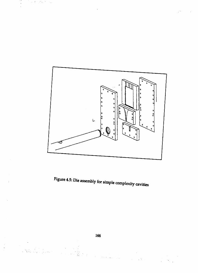
Figure 4.5: Die assembly for sii•r simple complexity cavities

166

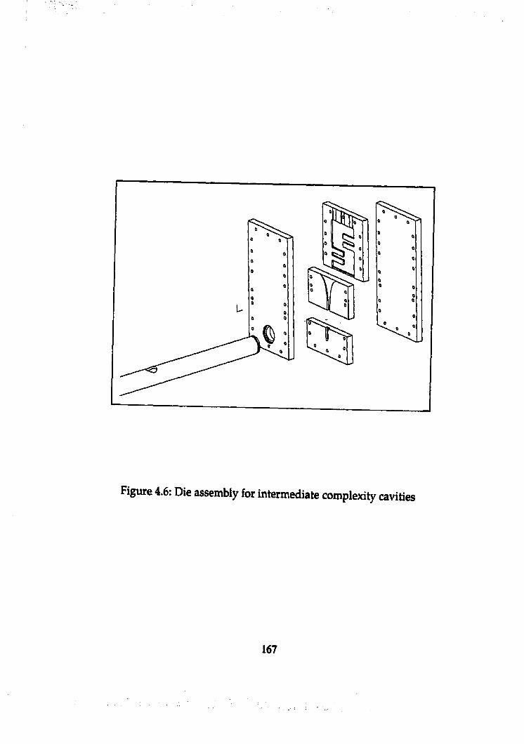
Figure 4.6: Die assembly for intermediate complexity cavities

167

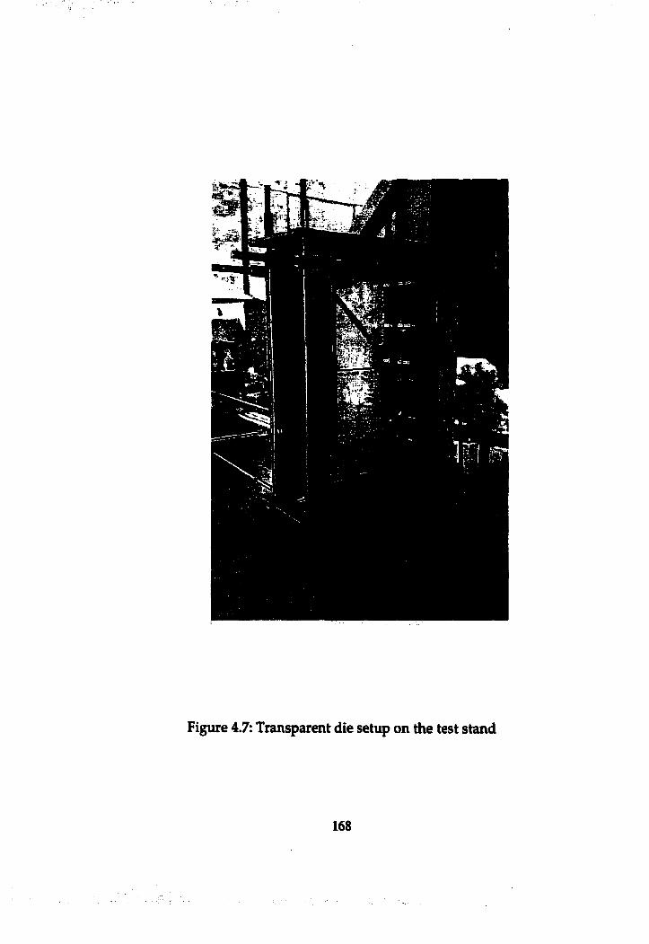
Figure 4.7: Transparent die setup on the test stand

168

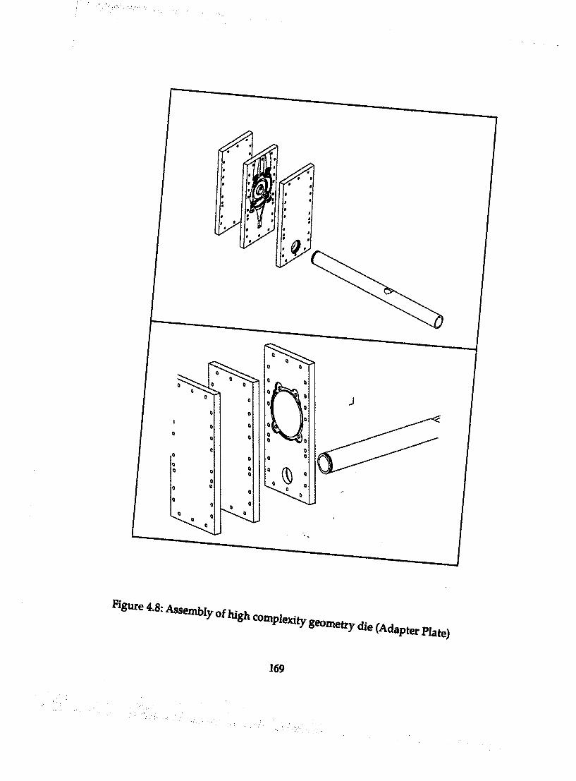
Figure 4.8: Assembly of high“ oiptexilygeomehydiefAd PterPlate)

169

4.4 Experimental setup

As a die casting analogy system. Prince test stand with Visi-Trak system,

which is available at NSM Lab at The Ohio state University, was used for

water analog tests (Figure 4.9). The hydraulic system with maximum 3,000

psi pressure accumulator, which controls plunger velocity and acceleration,

was monitored and controlled by Visi-Trak control system. With the

capability of easily programmable velocity/position setup (i.e. maximum 6

vel./pos. set points), the Visi-Trak system provided convenient and flexible

shot profile modification. Also, Visi-Trak control system receives position

feedback hom the shot cylinder for closed loop control. To ensure the

accuracy of shot cylinder position, a magnetic position sensor encoder is

utilized.

Although Visi-Trak control system provided convenience and flexibility

in programming and accuracy in position control using feedback system, its

capability was affected by the hydraulic system of Prince test stand. For

example, once hydraulic oil heated up during the experiment, plunger speed

increased in the same valve opening due to the changes of viscosity of

hydraulic oil. This condition limited the consistent control of plunger

velocities.

170

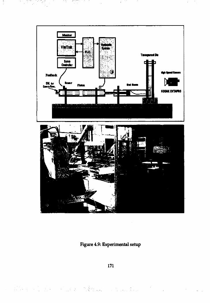
— >v w #

P tfci

Sino ' f 'Cinlnlir

TmipmnlDli

SW.hrCHm i i I i m .

/ 1 - m

Figure 4.9: Experimental setup

171

To catch the image of cavity flow with very high velocity, a high-speed

camera, Kodak EKTAPRO 4540- HS Motion Analyzer was used (Figure 4.10).

The recording rate used in this experiment was 4500 hames per second and

the stored digital images were recorded in Super-VHS tapes.

Since cavity fill time is very short (i.e. plunger speed is very high), limit

switch was attached on the cylinder rod to turn on the camera

instantaneously as soon as flow All the runner.

172

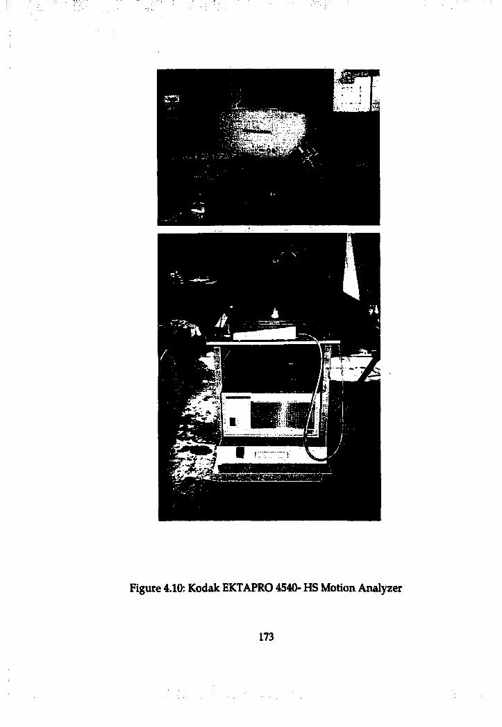
Figure 4.10: Kodak EKTAPRO 4540- HS Motion Analyzer

173

4.5 Dynamic sim ilarity

As mentioned in chapter, 2.5.3, physical flow models need dynamic

similarity to actual flow systems. Cavity flow is free surface flow. For the

physical similarity of free surface flow, three different dimensionless

numbers are supposed to be taken into account, i.e., Reynolds number,

Froude number, and Weber number.

Among those three different dimensionless numbers, Froude number,

which is associated with gravity force, was naturally the same in this

physical simulation. Regarding Weber number, surface tension of molten

aluminum is about 10 times higher than surface tension of water used (Table

2.3). However, Weber number was ignored in this experiment since cavity

flow has very high inertia as compared to surface tension. The Weber

number is important only if it is order unity or less [White, 79] (Equation

2.21).

However, for this physical flow simulation, Reynolds number should be

taken care of. There is a difference in fluid density between water and

molten alloy (aluminum) as water is used as a replacement for molten alloy,

such as molten aluminum (Table 2.3). Therefore, for the similarity of fluid

density, glycerin 7% by weight was added to water. Using the glycerin

solution water, the viscosity of solution water is also almost same as that of

molten aluminum: kinematic viscosity of solution water is 0.0117 stokes at 18

174

“c and kinematic viscosity of molten aluminum at 700 °c is 0.0116 stokes

[Duran, 91].

4.6 Water model vs. Computer model

To evaluate computer flow models developed using Flow3D,

correlations between water model results and computer model results were

investigated using three different complexity geometry of die cavities: 1)

simple plate die cavity, no cavity pre-fill, 1187 in/sec (=3014.98 cm/sec) of

fast shot gate velocity, and 22 ms of transition time from slow to fast shot

(Figure 4.11), 2) intermediate complexity geometry die cavity, 20% cavity

pre-fill with pre-fill velocity of 292.49 in/sec (=742.92 cm/sec), 1132 in/sec

(2875.28 cm/sec) of fast shot gate velocity, and 21 ms of transition time from

slow to fast shot (Figure 4.12), and 3) high complexity geometry die cavity,

no pre-fill, 1396 in/sec (=3545.84 cm/sec) of fast shot gate velocity, and 20

ms of transition time from slow to fast shot (Figure 4.13).

The next three figures show flow sequence of the two different cavity

flow models developed using the same geometry and process parameters

described above (i.e.. Water models vs. Computer flow models).

175

■■ ’ -

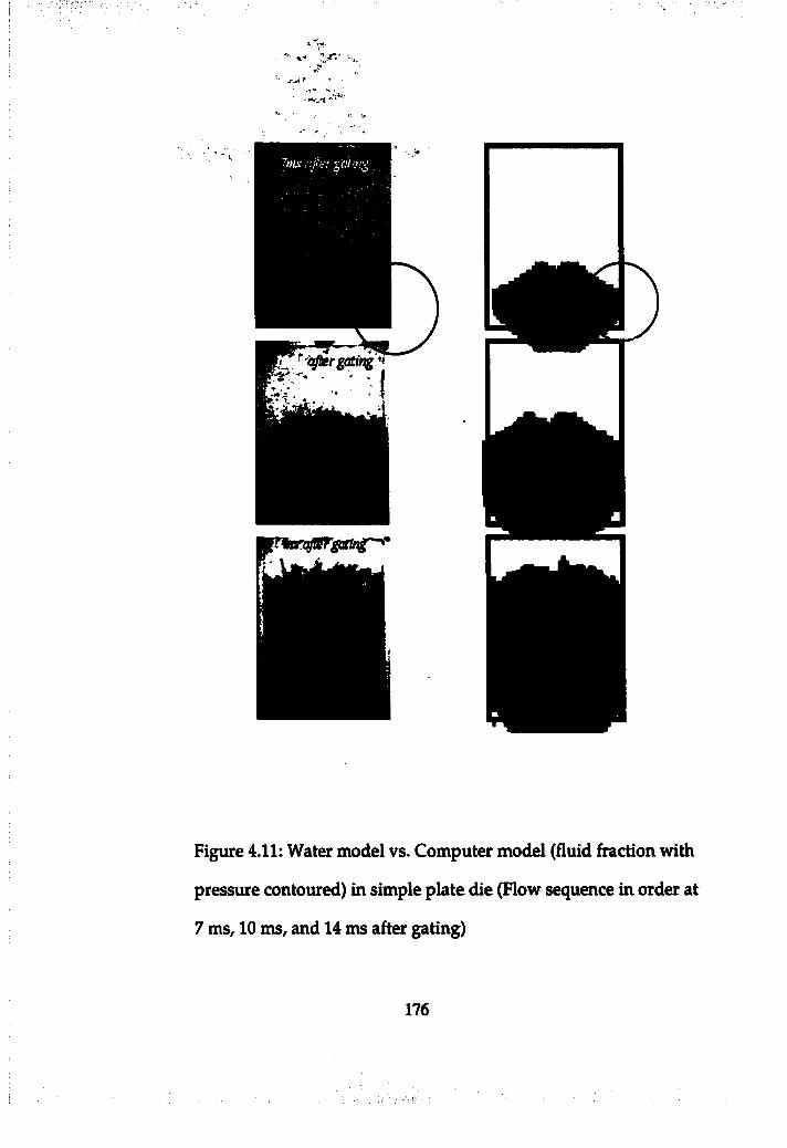
rjU.

I ■■ cfiergqting*f

I ' ; - . ' : ' !

Figure 4.11: Water model vs. Computer model (fluid fraction with

pressure contoured) in simple plate die (Flow sequence in order at

7 ms, 10 ms, and 14 ms after gating)

176

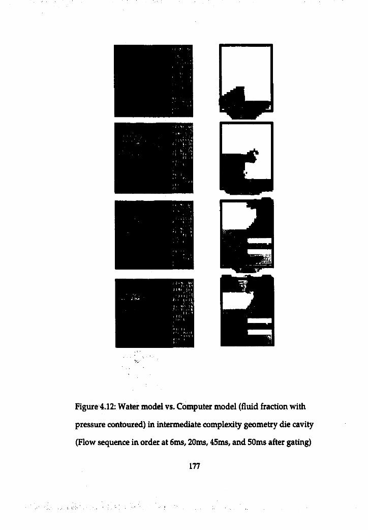
Figure 4.12: Water model vs. Computer model (fluid fraction with

pressure contoured) in intermediate complexi^ geometry die cavity

(Flow sequence in order at 6ms^ 20ms, 45ms, and 50ms after gating)

177

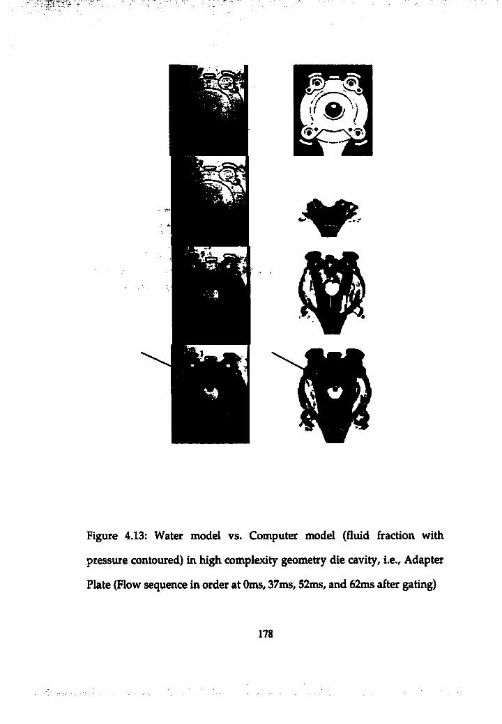
I

Figure 4.13: Water model vs. Computer model (fluid fraction with

pressure contoured) in high complexity geometry die cavity, i.e.. Adapter

Plate (Flow sequence in order at 0ms, 37ms, 52ms, and 62ms after gating)

178

- ' Y "The above three figures show good correlations between water models

and computer flow models. In Figure 4.11, fold-over of jet flow sheet right

after collision with both side walls in the die cavity was well simulated in

computer flow model. Also, in figure 4.13, eye-like air pocket in water

model was clearly shown in the computer flow model.

However, unfortunately, since only two-dimensional images in water

models were available, computer flow models predicting development and

behavior of jet flow sheet were not evaluated (e.g. the thickness of the flow

sheet) even though three-dimensional computer models of the flow patterns

were available.

179

CHAPTERS

COMPUTER EXPERIMENT

Upon obtaining good correlations between the computer and water

analog cavity filling patterns (Chapter 4), and between quantitative

estimation using computer flow models and experimental results (Chapter

3.3), a computer experiment was conducted using computer generated

design of experiment (DOE) to investigate the effect of both injection and

geometry parameters associated with cavity pre-fill on air entrapment in the

die cavity.

5.1 Modeling

In the computer experiment, three-dimensional models were employed.

The basic assumptions, critical slow plunger velocity, and fast shot velocity

were the same as used in three-dimensional computer flow models in

Chapter 3.2.

180

5.2 Parameters investigated

Based on the results of two-dimensional and three-dimensional

computer flow models (Chapter 3), parameters associated with cavity pre-fill

were selected to investigate their effects on air entrapment in the die cavity.

The parameters were divided into two categories. One was 'injection

parameters' and the other one was 'geometry parameters' including

locations and areas of gates and vents.

5.2.1 Injection parameters

Injection parameters were: 1) cavity pre-fill percentage, 2) transition time

from slow to fast shot velocity, and 3) cavity pre-fill slow shot velocity. The

significance of the effects of the above three injection parameters on air

entrapment were observed in two-dimensional computer flow models in

Chapter 3.1.

5.2.2 Geometry parameters

Unlike injection parameters, geometry had to be parameterized for the

quantitative analysis. The geometry parameters were: 1) ratio of gate

thickness and width to total casting thickness and width, 2) gate an^e, and 3)

flow disturbance (or complexity of die geometry).

181

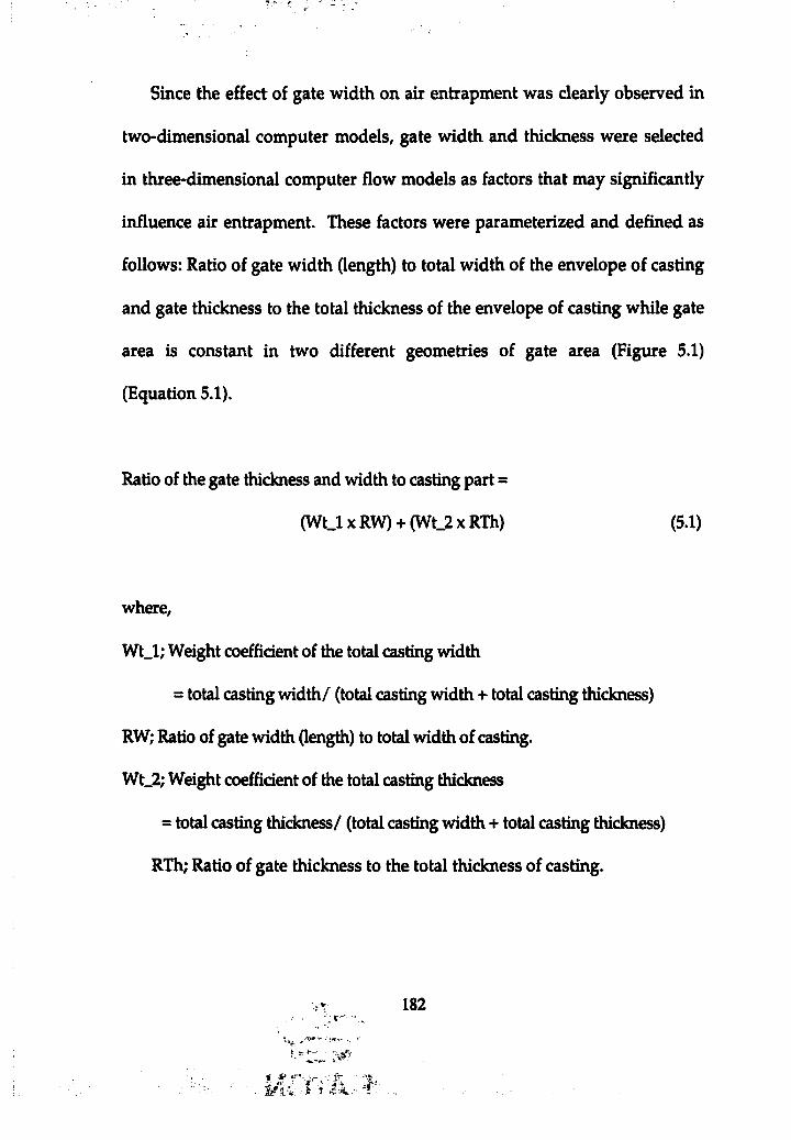
Since the effect of gate width on air entrapment was clearly observed in

two-dimensional computer models, gate width and thickness were selected

in three-dimensional computer flow models as factors that may significantly

influence air entrapment. These factors were parameterized and defined as

follows: Ratio of gate width (length) to total width of the envelope of casting

and gate thickness to the total thickness of the envelope of casting while gate

area is constant in two different geometries of gate area (Figure 5.1)

(Equation 5.1).

Ratio of the gate thickness and width to casting part =

(Wt_lxRW) + (Wt_2xRTh) (5.1)

where,

Wt_l; Weight coefficient of the total casting width

= total casting w idth/ (total casting width + total casting thickness)

RW; Ratio of gate width (length) to total width of casting.

Wt_2; Weight coefficient of the total casting thickness

= total casting thickness/ (total casting width + total casting thickness)

RTh; Ratio of gate thickness to the total thickness of casting.

182

Total width Total thickness

Figure 5.1: Total width and thickness of casting

1 8 3

For example, if cavity geometry used in chapter 3.2.1 (the cavity with 5 in. of

total casting width & 0.5 in. of total thickness) is selected and two different gate

dimensions are 3.65 in. x 0.04 in. and 2 in. x 0.073 in. (0.146 in^ of same area),

'Ratios of gate thickness and width to casting' for each different gates are:

(Relatively) wide & thin gate area (i.e. 3.65 in. X 0.04 in.)

[(5/5.5) X 73%] + [(0.5/5.5) x 8 % ] = 67%

(Relatively) narrow & thick gate area (2 in. x 0.073 in.)

[(5/5.5) X 40%] + [(0.5/5.5) x 15%] = 38%

In addition, since differences in flow patterns were found in three-

dimensional flow model using two different runners (i.e. angled fan gate and

chisel gate) (Qiapter 3.2), 'Gating angle' was selected as another geometry

parameter. Gating angle was defined as the angle between gating jet flow line

and the tangential line to the adjacent casting at the contact point of gate and the

adjacent casting part.

It was observed that the obstacles in the die cavity changed of the directions

of high inertia metal jet flow and increased turbulence of cavity flow.

Accordingly, the degree of flow disturbance was highly suspected to be another

significant geometry factor influencing filling patterns and consequently air

184

entrapment in the die cavity. Based on the locations of gates and vents, the

degree of flow disturbance is estimated. Conceptually, this parameter represents

the complexity of die cavity or flow detour distance during its travel from gates

to vents.

FD (Degree of Flow Disturbance) = Dtravei / DteucUdeaa (5.2)

where,

Dtiavei = Minimum flow travel distance from imaginary gate to one selected

vent

DEudidean = Minimum distance from imaginary gate to one selected vent in

Euclidean three-dimensional space.

The procedure to find the FD value is 1) one vent and one gate that are the

furthest apart in Euclidean three-dimensional space are selected. The distance

between gates and vents is examined from the centroid of the vent entry area

to the centroid of the gate entry area, 2) imaginary gate is located where a

selected gate is located, with maximum possible width (or length). The

maximum possible size of gate width (or length) is a maximum possible width

(or length) of adjacent casting where the imaginary gate can be attached. The

type of the gate is assumed be a straight chisel gate with no angle, 3) DEucUdean

185

is the shortest distance 6om the centroid of the selected vent entry area to the

line that imaginary gate lies on the casting. Basically, this distance is the

shortest distance from one point to the line, 4) Duavei can be measured by

using a function of Castview®, i.e. fill distance analysis (Figure 5.2).

For instance, for two different cavity geometries (simple plate die cavity

and cavity with ribs) in Figure 3.20 and Figure 5.2, a selected vent is obviously

a vent at the left or right hand side among three. In both the simple plate die

cavity and cavity with ribs (12.7 cm x 17.78 cm x 1.27 cm or 5 in x 7 in x 0.5 in),

DEudidean is 17.78 cm (or 7 in) since the distance from the imaginary gate and

the selected vent are the same. In simple die cavity, estimated Dtravei was also

17.78 cm (or 7 in) (Figure 5.2). Therefore, the value of the parameter, 'degree

of flow disturbance' is 1. The parameter, value of 1 means that the gating

flow is not disturbed in the die cavity during its travel from gates to the vents,

i.e. no obstacles on the flow path in the die cavity. However, in the cavity

with ribs, the parameter, degree of flow disturbance' is estimated to be 1.36.

The value is bigger than 1 since gating jet flow is disturbed by the obstacles,

the ribs inside the die cavity (Figure 5.2). It should be noted that the value of

the parameter, 'degree of flow disturbance' can't be obtained without the

locations of gates and vents, while actual gate size or geometry is not

necessarily known.

186

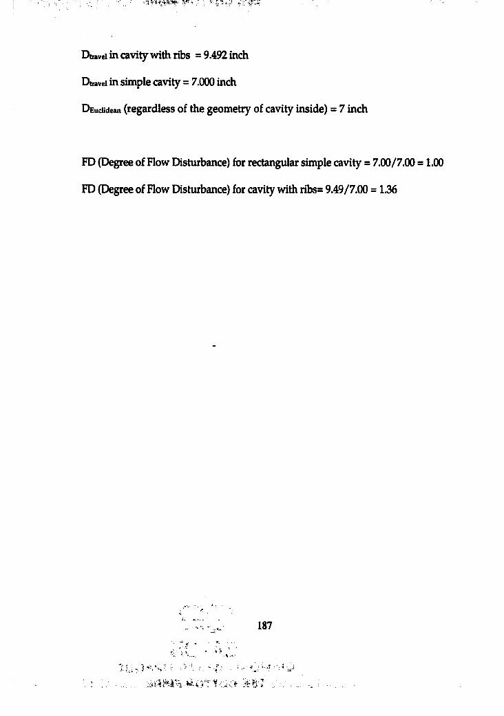
Dbavei in cavity with ribs =9.492 inch

Dtiavei in simple cavity = 7.000 inch

DEudidean (regardless of the geometry of cavity inside) = 7 inch

FD (Degree of Flow Disturbance) for rectangular simple cavity = 7.00/7.00 = 1.00

FD (Degree of Flow Disturbance) for cavity with ribs= 9.49/7.00 = 1.36

187

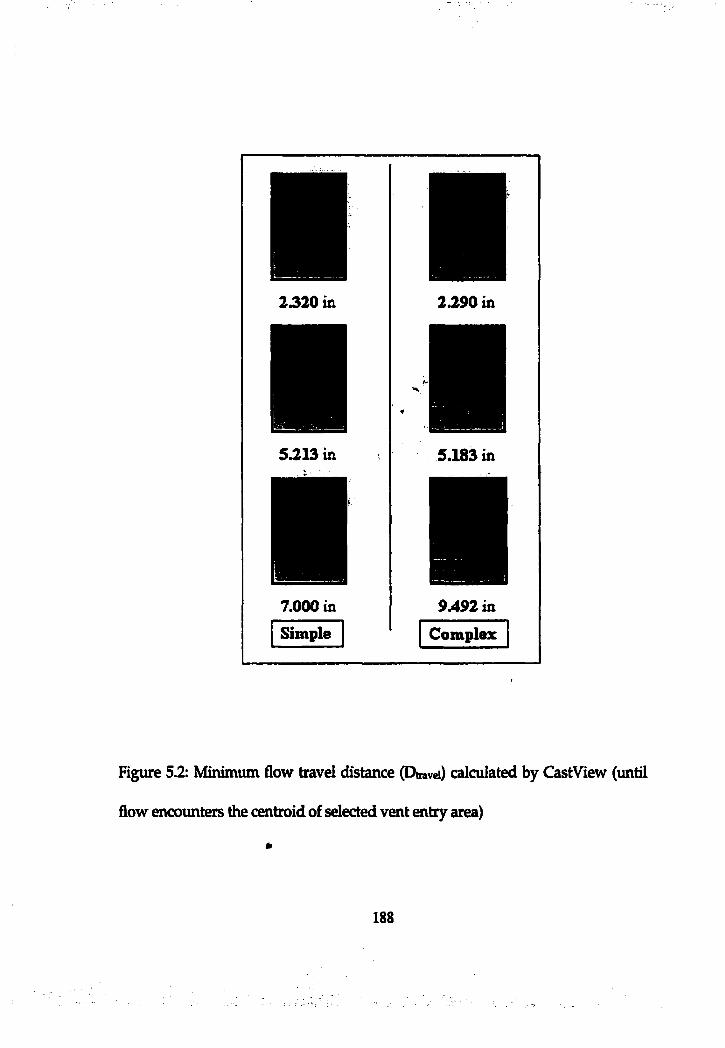
2.320 in

5.213 in

7.000 in

Sim ple

2.290 in

5.183 in

9.492 in

C om plex

Figure 5 .2 : Minimum flow travel distance (Dhavei) calculated by CastView (until

flow encounters the centroid of selected vent entry area)

188

The parameter of Tlow disturbance' was developed to quantify the degrees

of the complexify of cavity geometries associated with air entrapment in the die

cavity. However^ it should be noted that the parameter of Tlow disturbance' is

limited to apply to predict the amount of air entrapment due to unlimited

number of various cavity geometries. The details will be discussed in Chapter

5.4.

To investigate the effect of the above three geometry parameters on filling

patterns, two different die cavities and four different gates were designed (Figure

5.3,5.4,5.5,5.6).

189

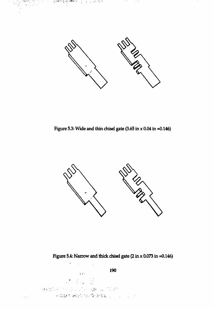
’-'"«tS •' Z.' i;_" « '

Figure 5.3: Wide and thin chisel gate (3.65 in x 0.04 in =0.146)

Figure 5.4: Narrow and thick chisel gate (2 in x 0.073 in =0.146)

190

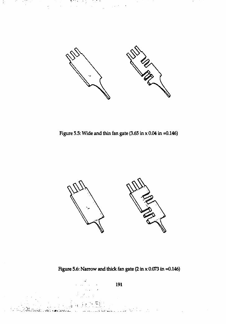
Figure 5.5: Wide and thin fan gate (3.65 in x 0.04 in =0.146)

Figure 5.6: Narrow and thick fan gate (2 in x 0.073 in =0.146)

191

The ranges of the above six parameters were determined based on previous

computer flow models and industry practices. The selected parameters was

named as follows: Transition time (TT), Cavity pre-fill (CP), Pre-fill velocity (PV),

Ratio of gate area to casting (GW), Gate angle (GA), and Flow Disturbance (FD)

(Table 5.1).

192

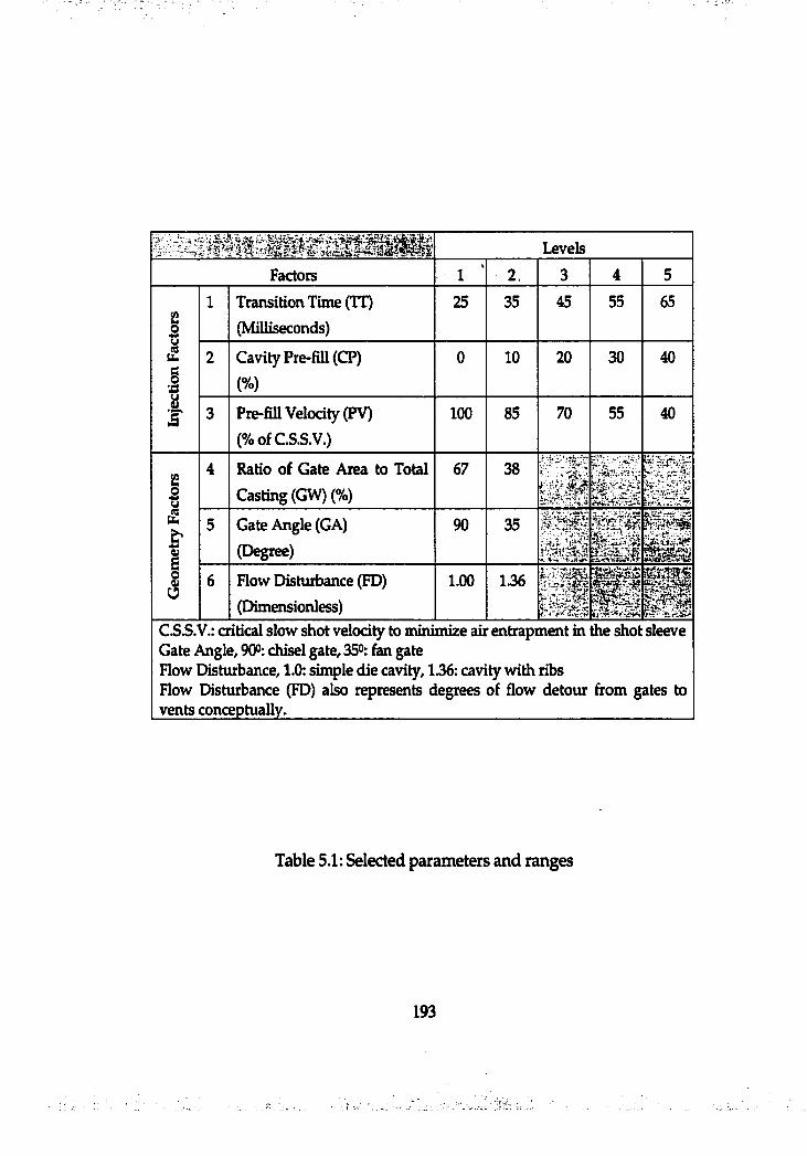
Levels

Factors 1 2 3 4 5

1t

1 Transition Time (IT) (Milliseconds)

25 35 45 55 65

2 Cavity Pre-fill (CP) (%)

0 10 20 30 40

3 Pre-fill Velocity (PV) (%ofC.S.S.V.)

100 85 70 55 40

1Î

4 Ratio of Gate Area to Total Casting (GW) (%)

67 38

illKîsBH

w ' V5 Gate Angle (GA)

(Degree)90 35 a K

6 Flow Disturbance (FD) (Dimensionless)

1.00 1.36 il■C.S.S.V.: critical slow shot velocity to minimize air entrapment in the shot sleeveGate Angle, 90°: chisel gate, 35°: fan gateFlow Disturbance, 1.0: simple die cavity, 1.36: cavity with ribsFlow Disturbance (FD) also represents degrees of flow detour from gates tovents conceptually.

Table 5.1: Selected parameters and ranges

193

5.3 Design of ex^erin^tiD O E)I, ,. '

* ' ’ V *

Two level fractTonâC factorial designs do not give information about

quadratic curvature or interactions of parameters (or factors). In general,

three level fractional factorial designs require very large number of runs.

Computer generated DOE makes sense for computer experiments instead

of Box Behnken designs and central composite designs found in Minitab. This

follows because they give more flexibility to allow the nesting of factors and

the fitting of specialized models, which make sense for computer experiments.

Types of computer generated designs include D-optimal, minimum bias, and

expected integrated mean squared error (EIMSE) optimal.

For this computer experiment, employing computer generated DOE

using EIMSE criterion, 40 runs of the DOE array were generated (Appendix

D). Any other pre-tabulated response surface designs, e.g., composite designs

or Box Behnken designs, would not allow to achieve the desired 'split plot'

structure of this computer experiment (Table 5.1). The 'split plot' means a

structure that includes exactly 8 specified combinations of the geometric

parameters in this experiment (Table 5.1), which are pre-spedfied to minimize

the time in geometric modeling. The spit plot structures are one of the most

important 'nested' design structures.

The EIMSE generalizes the well-known integrated mean squared error

(IMSE) criterion, using a distribution over a finite set of possible true models

194

to yield an estimate of the expected squared 'plus or minus' errors of

prediction.

EIMSE criterion

"In response surface methodology (RSM), the central issue is to uncover

the relationship y = q (x) between k design variables x = (xi, X2, Xk) and

response variable y. Although r\ is unknown, a fundamental assumption in

RSM states that the real world system is smooth enough that ii can be

approximated by a low order polynomial f(x) in k variables. With the basic

assumption, the form or order of polynomial should be spedhed before

planning the experiment [Myers, 95]. This makes the design selection via

criteria strongly depend upon the proposed form of f(x), such as "D-optimal"

design of experiment. In other words, there should be some concern about

possible bias due to model mis-spedfication. On the other hand, "minimum

bias" designs differ markedly hrom those implied by traditional optimality

criteria, which consider only functions of the variance. However, minimum

bias designs may give rise to a high modeling error because of the

uncontrolled variance error.

The advantages of EIMSE criterion are the following. First, in all the

cases, standard criteria from the literature such as all bias or D-optimality,

were not able or applied singly to generate designs with comparable

195

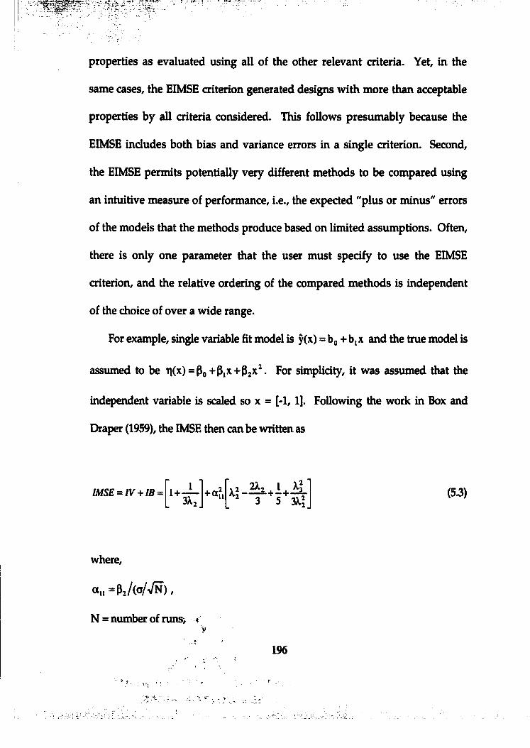
properties as evaluated using all of the other relevant criteria. Yet, in the

same cases, the EIMSE criterion generated designs with more than acceptable

properties by all criteria considered. This follows presumably because the

EIMSE includes both bias and variance errors in a single criterion. Second,

the EIMSE permits potentially very ditierent methods to be compared using

an intuitive measure of performance, i.e., the expected "plus or minus" errors

of the models that the methods produce based on limited assumptions. Often,

there is only one parameter that the user must specify to use the EIMSE

criterion, and the relative ordering of the compared methods is independent

of the choice of over a wide range.

For example, single variable fit model is y(x)= b + b,x and the true model is

assumed to be t](x) = Po tP^x+P^x^. For simplicity, it was assumed that the

independent variable is scaled so x = [-1,1]. Following the work in Box and

Draper (1959), the IMSE then can be written as

/W 5£ = /V + /B = 1+ - +af X"- 2X (5.3)

where,

a„ =P;/(o/Vn ) ,

N = number of runs;

196

Xi = i* moment of the design,

IV = integrated variance errors,

IB = integrated bias errors.

Box and Draper (1959) note that an might be interpreted as the ratio of the

curvature of the true model to the sampling error. When this ratio is quite small,

the optimal design will essentially minimize the variance term. Box and Draper

(1959) called this the "all variance " design. On the other hand, when this ratio is

quite large, the optimal design essentially minimizes the bias term, which is

called the " all-bias " design.

In the more usual case in which both bias and variance occur, the use of

IMSE as a design criterion, compared to the all-variance design or all-bias design

criterion, is considered to be appealing. An obvious reason is that it

simultaneously considers the variance and the bias of predicted values.

However, a design that minimizes IMSE is difficult to find since the knowledge

of the unknown coefficient of the missing term (in this case, Pz) is needed. Box

and Draper (1959) avoid this difficulty by showing that over a very wide range of

values of On, any all-bias design that completely ignores the variance errors

comes very dose to mfimmzmg IMSE. This approach tries to cover different

values of a,!, which is in fact determined based on Pz, the unknown coeffident of

the missing term in this simple example.

197

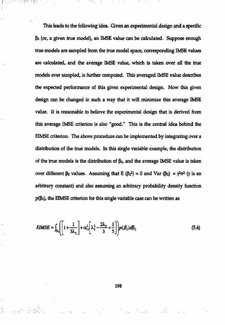
This leads to the following idea. Given an experimental design and a specific

Pz (or a given true model), an IMSE value can be calculated. Suppose enough

true models are sampled from the true model space, corresponding IMSE values

are calculated, and the average IMSE value, which is taken over all the true

models ever sampled, is further computed. This averaged IMSE value describes

the expected performance of this given experimental design. Now this given

design can be changed in such a way that it will minimize this average IMSE

value. It is reasonable to believe the experimental design that is derived from

this average IMSE criterion is also "good." This is the central idea behind the

EIMSE criterion. The above procedure can be implemented by integrating over a

distribution of the true models, fri this single variable example, the distribution

of the true models is the distribution of Pz, and the average IMSE value is taken

over different Pz values. Assuming that E (Pf) = 0 and Var (Pz) = (Y is an

arbitrary constant) and also assuming an arbitrary probability density function

p(Pz), the EIMSE criterion for this single variable case can be written as

£ Z M 5 E = frr

1+ -3X ,

+ a P(A)dPî (5.4)

198

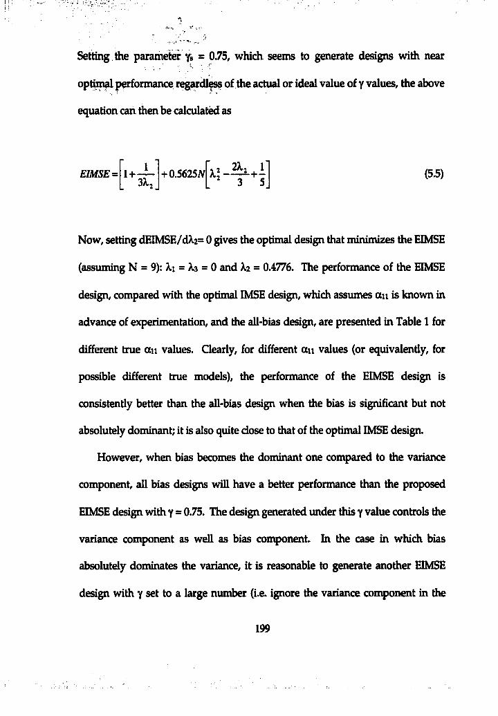
Setting the parameter y» = 0.75, which seems to generate designs with near■ . 'i - •

optunal performance reg a rd l^ of the actual or ideal value of y values, the above

equation can then be calculated as

EIMSE = I+-7- +0.56253Xj . 3 5.

(5.5)

Now, setting dEIMSE/dXz^ 0 gives the optimal design that minimizes the EIMSE

(assuming N = 9): Xi = Xa = 0 and Xz = 0.4776. The performance of the EIMSE

design, compared with the optimal IMSE design, which assumes an is known in

advance of experimentation, and the all-bias design, are presented in Table 1 for

different true an values. Clearly, for different a n values (or equivalently, for

possible different true models), the performance of the EIMSE design is

consistently better than the all-bias design when the bias is significant but not

absolutely dominant; it is also quite close to that of the optimal IMSE design.

However, when bias becomes the dominant one compared to the variance

component, all bias designs will have a better performance than the proposed

EIMSE design with y = 0.75. The design generated under this y value controls the

variance component as well as bias component In the case in which bias

absolutely dominates the variance, it is reasonable to generate another EIMSE

design with y set to a large number (i.e. ignore the variance component in the

199

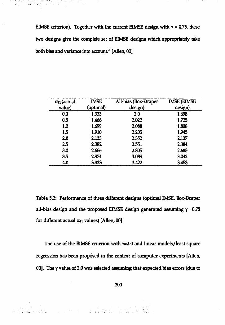
EIMSE criterion). Together with the current EIMSE design with y = 0.75, these

two designs give the complete set of EIMSE designs which appropriately take

both bias and variance into account." [Allen, 00]

ail (actual value)

IMSE(optimal)

All-bias (Box-Draper design)

IMSE (EIMSE design)

0.0 1.333 2.0 1.6980.5 1.466 2.022 1.7251.0 1.699 2.088 1.8081.5 1.910 2.205 1.9452.0 2.133 2.352 2.1372.5 2.382 2.551 2.3843.0 2.666 2.805 2.6853.5 2.974 3.089 3.0424.0 3.333 3.422 3.453

Table 5.2: Performance of three different designs (optimal IMSE, Box-Draper

all-bias design and the proposed EIMSE design generated assuming y =0.75

for different actual a n values) [Allen, 00]

The use of the EIMSE criterion with y=2.0 and linear models/least square

regression has been proposed in the context of computer experiments [Allen,

00]. The y value of 2.0 was selected assuming that expected bias errors (due to

200

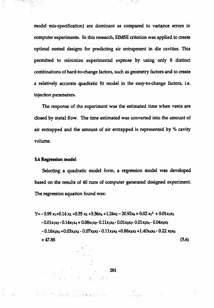
model mis-spedfication) are dominant as compared to variance errors in

computer experiments. In this research, EIMSE criterion was applied to create

optimal nested designs for predicting air entrapment in die cavities. This

permitted to minimize experimental expense by using only 8 distinct

combinations of hard-to-change factors, such as geometry factors and to create

a relatively accurate quadratic fit model in the easy-to-change factors, i.e.

injection parameters.

The response of the experiment was the estimated time when vents are

closed by metal flow. The time estimated was converted into the amount of

air entrapped and the amount of air entrapped is represented by % cavity

volume.

5.4 Regression model

Selecting a quadratic model form, a regression model was developed

based on the results of 40 runs of computer generated designed experiment.

The regression equation found was:

Y= - 0.99 x i+0 .14 X2 +0.55 xa +5.56x4 +1.24x5 - 20.92x6 + 0.02 xi^ + 0.01xiX2

- O.Olxixa - 0.14x1X4 + O.OSxixs- O .llxixe - 0.01x2X3- 0.01x2X4 - 0.04x2X5

- 0.16X2X6 +0.03X3X4 - 0.07X3X5 - 0.11X3X6 +0 .86x4X5 +1.40X4X6 - 0 .2 2 X5X6

+ 47.88 (5.6)

201

Response;

Y: Amount of Air Entrapment, % Cavity Volume

Process Parameters;

XI: Transition Time (TT) (25 ~65) ms

X2: Percentage Cavity Pre-fill (CP) (0 - 40)%

X3: Cavity Pre-fill Velocity (PV) (100-40)%

Geometry Parameters;

X4: Gate Width (GW) (coded, l=Narrow, -l=Wide)

xs: Gate Angle (GA) (coded, l=Straight, -l=Fan)

X6: Flow Disturbance (FD) (or Complexity of Cavity Geometry)

(Coded, l=Complex, -l=Simple)

The significance of main effects and interactions among selected factors

were determined based on the P values of factors using Minitab (Appendix I).

The main effect of complexity of cavity geometry (i.e. flow disturbance (FD))

was the most significant factor influencing the amount of air entrapment

(Appendix J) and intera(^on of cavity pre-fill velocity & complexity of

geometry was the next The other significant factors were, in order, the main

effect of cavity pre-fill percentages, the mteraction of cavity pre-fill &

complexity of geometiy, the interaction of transition time & cavity pre-fill

202

velocity, the interaction of cavity pre-fill & cavity pre-fill velocity, and the

interaction of transition time & gate width and thickness ratio to casting. It

was found that, in general, interactions of selected factors more significantly

influenced air entrapment than main effects. In other words, an appropriate

combination of factors, such as transition time & cavity pre-hll velocity could

help reduce the amount of air entrapment in die cavities. This was also

observed in 2D computer models. In two dimensional rectangular simple

geometry of cavity with narrow straight gate, employing injection parameters

of 10 % pre-fill with 30 ms transition time, 20% pre-fill with 20 ms transition

time, and 30% pre-fill with 10 ms transition time generated the best cavity fill

pattern in terms of air entrapment.

203

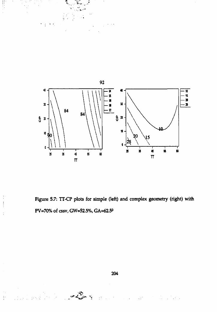
t.

924 0 H — 84

a.u

25 35 45 55 65

40-1

CLU

lo­

ss35 45 5525

TTTT

— 10 — 15 — 20 — 20

Figure 5.7: TT-CP plots for simple (left) and complex geometry (right) with

PV=70% of cssv, GW=52.5%, GA=62.5<>

204

''H-

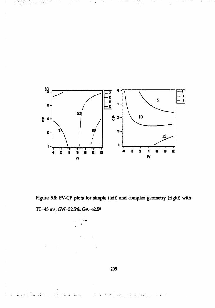
— 0

:: -— ;— 10 — 15

3 0 -

S&U

1 0 -

« 90 00 10 a n 100« a 01 n H « 100PV PV

Figure 5.8: PV-CP plots for simple (left) and complex geometry (right) with

TT=45 ms, GW=52.5%, GA=62.50

205

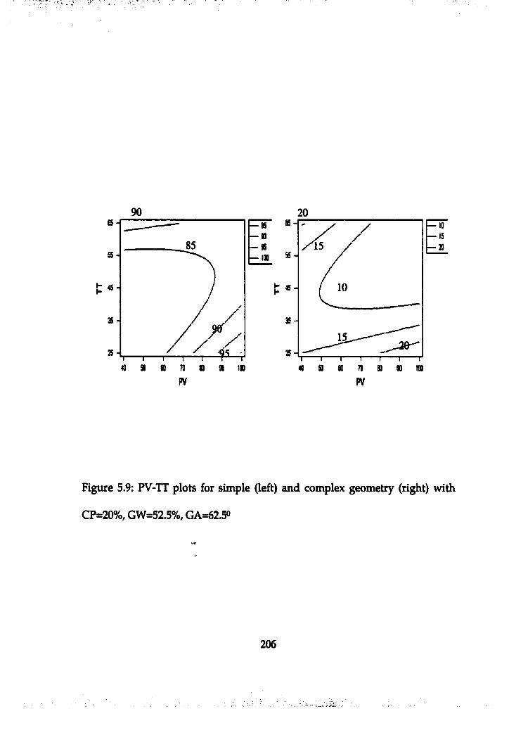
90 2 0(S

t «

7S

40 91 m 70 m 90 im

8S -*— 85— 9D— 95

— 10 — 15

100

c

39-

29-40 90 90 70 80 90 lOO

PV PV

Figure 5.9: PV-TT plots for simple (left) and complex geometry (right) with

CP=20%, GW=52.5%, GA=62.5«

206

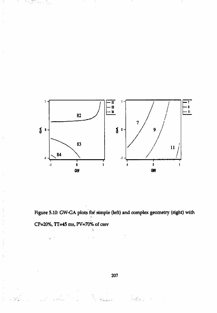
— 9— 92— 83— U

i “5 “

-1-I00-I

GW GW

Figure 5.10: GW-GA plots fôf simple (left) and complex geometry (right) with

CP=20%, TT=45 ms, FV=70% of cssv

207

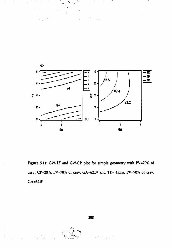
92

3 S -

% -0

869890 30-

— 92

Q.0

82.2

90

— 022 824

1— 0 2 6

GW GW

Figure 5.11: GW-TT and GW-CP plot for simple geometry with FV=70% of

cssv, CP=2G%, PV=70% of cssv, GA=62.5° and TT= 45ms, PV=70% of cssv,

GA=62.50

208

' ' ?-T.'

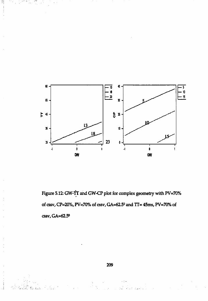
fis-I — 13 — 5— 10 — 15

18— 23

30 -

a.0

35 -

230 0

GW GW

Figure 5.12: GW-TT and GW-CP plot for complex geometry with PV=70%

of cssv, CP=20%, PV=70% of cssv, GA=62.5° and TT= 45ms, PV=70% of

cssv, GA=62.5°

209

As observed from the above contour plots (from Figure 5.7 to 5.12) of the

regression model developed, the amount of air entrapment was predicted to

be much less in this complex die cavity (from Figure 5.3 to 5.6) (i.e. cavity

with ribs) than in the simple plate die cavity (from Figure 5.3 to 5.6). In the

complex die cavity, the direction of flow velocity vector was changed due to

the obstacles in die cavities, which caused time delay for molten metal flow

to reach and close vents.

It should be noted that contour plots from Figure 5.7 to 5.12 were drawn

by taking middle values of the selected ranges of the other parameters,

except complexity of cavity geometry.

In Figure 5.7, it is shown on the TT-CP plots that once transition time is

selected in the range of 40 ms to 50 ms in simple die cavity, percentage

cavity pre-fill hardly effects on the amount of air entrapment. However, in

complex geometry of cavity (cavity with ribs), the more cavity pre-fill is

used, the less amount of air is entrapped. The response was relatively

sensitive when shorter transition time (25 to 40 ms) is used. Also, it was

indicated that relatively less cavity pre-fill can be used to achieve 10% cavity

volume of trapped air at long transition time (45 to 60 ms). In the complex

die cavity with ribs inside, transition time between 50 and 60 ms and cavity

pre-fill more than 20% is desirable to minimize air entrapment.

2 1 0

Two different PV-CP contour plots. (Figure 5.8) show that in the simple

die cavity, the lowest pre-fill velocity with a little amount of cavity pre-fill is

desired. In contrast to the case of simple die cavity, a high percentage of

cavity pre-fill helps reduce air entrapment in the complex die cavity.

Especially with high pre-fill velocity, high cavity pre-fill (i.e. 30 to 40 %)

causes minimum air entrapment. However, high pre-fill velocity (more than

80% of critical slow shot velocity) with very little cavity pre-fill (e.g. less

than 10%) increases the amount of air entrapment.

Similar to the PV-CP plots, two plots of PV-TT (Figure 5.9) show the best

performance at low pre-fill velocity with shorter transition time in the

simple cavity, and at high pre-fill velocity with longer transition time in the

complex cavity. It should be noted that the effects of transition time (TT)

and cavity pre-fill (CP) on flow patterns were observed to be similar,

generating lateral expansion of flow, in the previous study using 2D

computer flow model.

In Figure 5.10, GW-GA plots show that the effects of their interaction on

air entrapment are insignificant. The response varies only 82-84% in the

simple cavity and 7-11% in the complex die cavity in the selected ranges of

the factors.

Form the plots in Figure 5.11, it can be concluded that in the simple die,

the interaction between GW and cavity pre-fill (CP) is insignificant, while

2 1 1

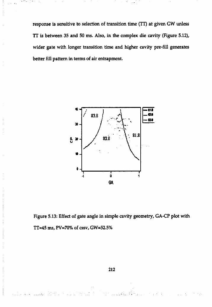
response is sensitive to selection of transition time (TT) a t given GW unless

TT is between 35 and 50 ms. Also, in the complex die cavity (Figure 5.12),

wider gate with longer transition time and higher cavity pre-fill generates

better fill pattern in terms of air entrapment.

3 0 -

m

1 0 -

0 1

%

Figure 5.13: Effect of gate angle in simple cavity geometry, GA-CP plot with

TT=45 ms, PV=70% of cssv, GW=52.5%

2 1 2

The effects of gate angle associated with cavity pre-fill on air entrapment

are shown in Figure 5.13. In the simple rectangular plate die cavity, the gate

angle associated with cavity pre-fill hardly effects air entrapment due to the

particular location of the gate and three y m fk ^

Limitations of the parameter, Flow Disturbance (FD)

As briefly mentioned in Chapter 5.2.2, unfortunately, there are limitations

to predict the amount of air entrapment in actual castings using the definition

of FD. For example, if vents are located very close to the gates in simple plate

die cavities (Figure 5.14), the FD value is 1 by the definition (regardless of the

gate width). The value of FD, 1 is the same value that is found when vents are

located on the top of the cavity. Even though all the values of parameters

including FD are the same as those parameter values in the case when vents

are located on the top of the cavity, the amount of air entrapment must be

different.

213

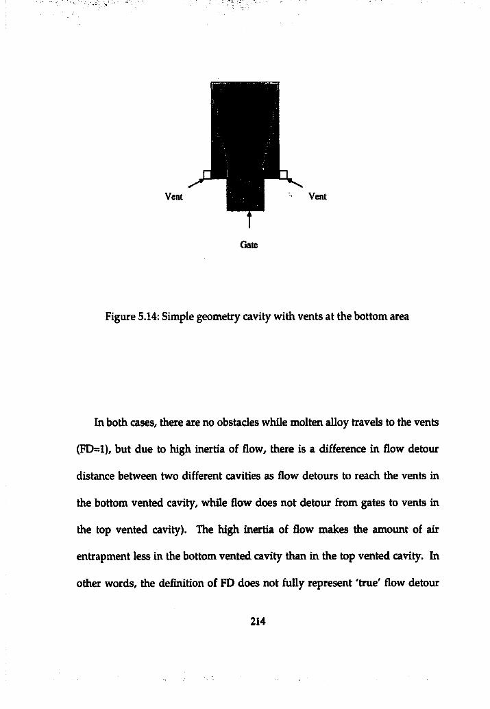
Vent Vent

Gate

Figure 5.14: Simple geometry cavity with vents at the bottom area

In both cases, there are no obstacles while molten alloy travels to the vents

(FD=1), but due to high inertia of flow, there is a difference in flow detour

distance between two different cavities as flow detours to reach the vents in

the bottom vented cavity, while flow does not detour hom gates to vents in

the top vented cavity). The high inertia of flow makes the amount of air

entrapment less in the bottom vented cavity than in the top vented cavity. In

other words, the definition of FD does not fully represent 'true' flow detour

214

(i.e., flow detour distance from gates to vents vs. distance form gates to vents

in Euclidean space).

Thus, in general, FD value is meaningful in the case that the direction of

velocity vector of initial gating flow through the imaginary gate (as defined in

Chapter 5.2.2) is toward the furthest vents from actual gates, also when multi­

gates are all located in the same side in the die cavity, so that imaginary gate,

which covers whole gate side, includes every actual gates.

The parameter, FD was developed to parameterize the degrees of

complexity of cavity geometries associated with cavity flow patterns. Even

though the value of FD obtained by the definition in Chapter 5.2.2 could not

generalize complexity of cavity geometries associated with cavity flow by the

numbers, understanding the modeling concept of complexity of cavity\ *

geometry associated cavity flow pattern or degree of flow disturbance from

gates to vents associated with cavity geometry will help determine optimum

injection parameters for the cavity pre-fill approach. Also, the regression

model associated with the FD is supposed to be interpreted in a qualitative

manner based on the concept of FD. It should be noted that the regression

model was developed based on only two different FD values, i.e., two

different complexity cavity geometries, or no flow disturbance (or no flow

215

- ■ -.-A-. -•

detour) vs. some degrees of flow disturbance (or some degrees of flow detour

from gates to vents).

5-5 Conclusions and discussion

Conclusions and discussion were drawn out of the results of models (the

computer flow models and regression model) developed under the

assumptions as previously stated, understanding the limitations of model

application, such as materials, cavity geometry including locations and types

of gates and vents, process conditions, and die casting machine capabilities.

1) As observed in 2D computer model, in 3D computer flow modeling, it was

observed that cavity pre-fill promoted unilateral expansion of cavity flow in

the die cavity. The lateral expansion of flow is a major beneficial physical

property, which generates more uniform cavity fill. The changes of filling

patterns by employing cavity pre-fill help reduce the amount of air

entrapment. More molten metal is filled before vents are blocked and sealed.

2) To maximize the beneficial effects of cavity pre-fill, an appropriate

combination of injection parameters, such as cavity pre-fill percentage,

transition time from slow to fast shot, and slow shot cavity pre-fill (gate)

velocity, should be employed. Cavity pre-fill approach with inapt

216

combinations of the injection and geometry parameters can possibly result in

more air entrapment than no cavity pre-fill.

3) Geometry factors are important factors influencing cavity fill patterns and

air entrapment in the die cavity. Especially, complexity of cavity geometry

associated with gate and vent locations, which is parameterized by flow

disturbance, FD, is the most significant factor (Appendix J).

Discussion

As estimated in this study, 80 to"'9Q5'o"ofi the cavity volume of air is

entrapped in the simple rectangular die cavity and less than 10 to 30% of

cavity volume of air is entrapped ia the cavity with some complexity (or some

degrees of flow disturbance).

Saying that 20% of the cavity volume is the estimated total amount of air

entrapment in the die cavity, which has some complexity as most actual

castings have, what is the volume of gas porosity? It should be noted that

air is compressible and the 20% of cavity volume is the air volume in

atmosphere before intensification pressure is engaged. In addition, this

value of air entrapment is overestimated assuming the vents are the only

way for air to escape. When it is assumed that intensification pressure is

engaged in the die cav i^ where air is trapped in, the volume of gas porosity

217

can be approximately calculated using ideal gas law. When 10,000 psi of

intensification pressure is exerted in the die cavity, the result is 0.029% of the. . - A ...

casting volume, which is the approximate volume of the gas porosity that

can be found. It is a very small percentage of the volume.

On the other hand, however, the complexity of cavity geometries can

cause specific constant defective (porosity related) local areas due to the

geometry itself, e.g. eddy circled areas due to the rapid change of flow

direction. This can cause concentration of air entrapment in the particular

area, which was observed in this study. Despite the amount of total air

entrapment is estimated very small, when the trapped air is concentrated in

the particular local area, the defect is noticeable and maybe most unwanted.

In this research, it was observed that the predictable defective area could be

improved by selecting appropriate combinations of different injection

parameters.

Accordingly, reducing the amount of air entrapment (gas porosity) in

particular local defective areas, the beneficial effects of cavity pre-fill might

be recognized in industry.

218

CHAPTER6

EXPERIMENTAL CASTINGS

Using cavity pre-fill, two different experimental castings were produced

to investigate the effects of cavity pre-fill on air entrapment. Molten alloy

was A1383 and the machine was a Prince cold chamber die casting machine.

6.1 Experiment 1

Figure 6.1 shows selected casting geometry for the experimental castings.

In the experiment, 0%, 30%, and 63% of cavity pre-fill were employed

(Figure 6.2). Critical slow shot velocity was used for the cavity pre-fill

velocity. Shot transition point ficom slow to fast shot was estimated based on

plunger diameter, amount of molten aluminum ladled in the shot sleeve,

runner volume, and cavity volume. Transition time firom slow to fast shot

had to be estimated based on the feedback shot profile since transition time

was set by hydraulic valve opening. Due to the noise of shot control system,

219

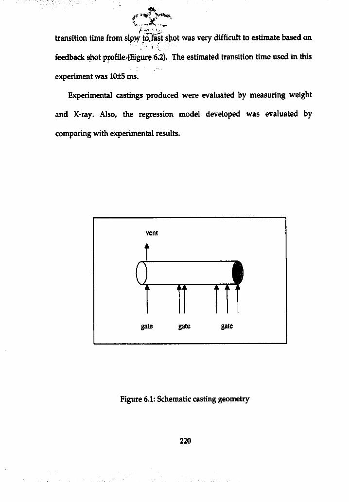
transition time from slpw to. fast shot was very difficult to estimate based on

feedback shot ppfUe^Eigure 6.2). The estimated transition time used in this

experiment was 10±5 ms.

Experimental castings produced were evaluated by measuring weight

and X-ray. Also, the regression model developed was evaluated by

comparing with experimental results.

gate

Figure 6.1: Schematic casting geometry

2 2 0

Maximum allowable cavify fill time

To ensure that delayed cavity fill time using cavity pre-fill is less than

the maximum allowable fill time, maximum allowable cavity fill time was

estimated based on cavity geometry using following equation based on

equation 2.6 in Chapter 2.

t = k X IX {[(Ti -If) + (S X Z)] / ( I f -Id)} (6.1)

where,

k: Alloy Constant (0.866 for Al)

I : Wall Thickness (0.125 to 0.75 in)

Ti: MetalTemperature (1260 °F)

Tf: Metal Flow Temperature (Minimum) (1060 °F)

Z: Temperature Equivalent (9.4 for Al 383)

Td: Die T e m p e ra te (300 <>F)

S: Percentage o l Solid (50 based on thickness)

The estimated maximum allowable cavity fill time was 446 ms based on

0.43 in. of wall thickness. By estimating cavity fill time when employing 63%

of cavity pre-fill. It was ensured that the cavity fill time was still within the

allowable fill time range. The estimated cavity fill time employing 63% of

cavity pre-fill was 218 ms.

2 2 1

Figure 6.2: Three different shot profiles for no pre-fill, 30%, and 63% cavity

pre-fill

2 2 2

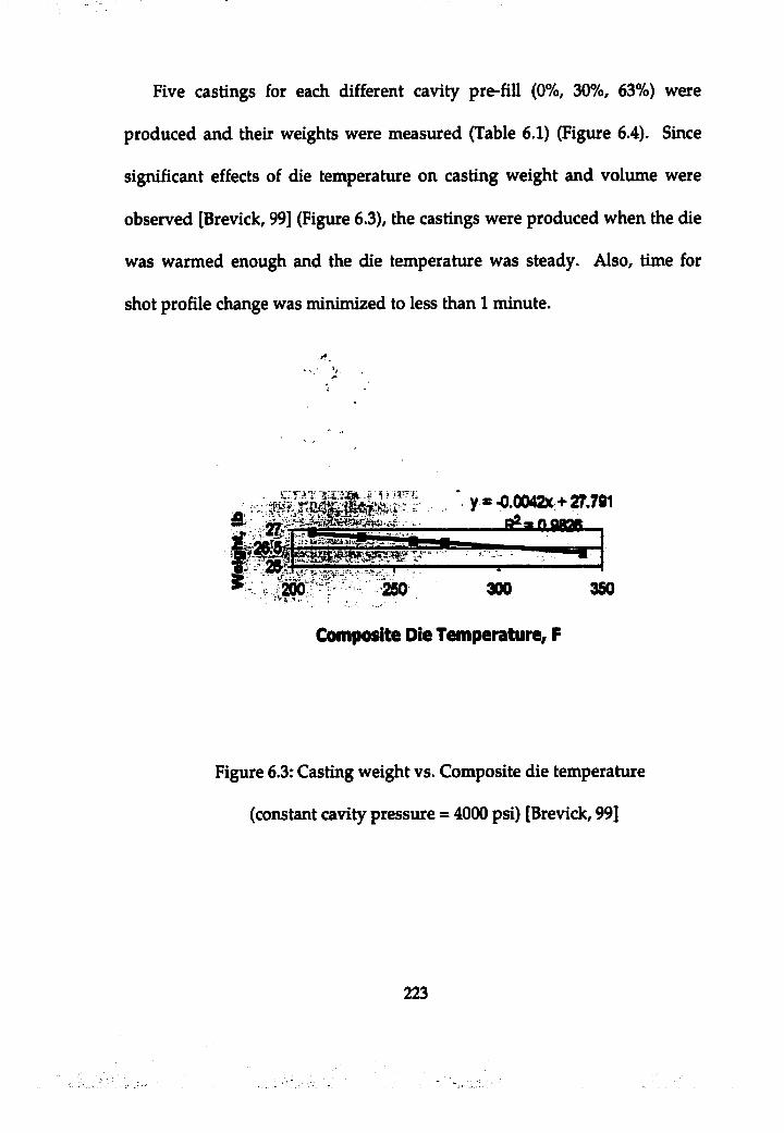
Five castings for each different cavity pre-fill (0%, 30%, 63%) were

produced and their weights were measured (Table 6.1) (Figure 6.4). Since

significant effects of die temperature on casting weight and volume were

observed [Brevick, 99] (Figure 6.3), the castings were produced when the die

was warmed enough and the die temperature was steady. Also, time for

shot profile change was minimized to less than 1 minute.

J* W

y s-0.0042x> 27.791

250 300 350

Composite Die Temperature, F

Figure 6.3: Casting weight vs. Composite die temperature

(constant cavity pressure = 4000 psi) [Brevick, 99]

223

Results

As can be seen in Table 6.1, more pre-fill produced castings with more

weight. In addition, using high cavity pre-fill (i.e. 63% of cavity pre-fill), the

variation of measures was small (in the range of 0.02 lbs) as compared to no

pre-fill and 30% pre-fill results.

Assuming that all the dimensions of the castings are the same, these

weights of the castings represent the density of the castings. The increased

density of the castings using cavity pre-fill indicated that the amount of

porosity in the castings were reduced. However, it was premature to

conclude that cavity pre-fill reduced the amount of gas porosity caused by

air entrapment in the die cavity as pronounced. Yet, it was unclear whether

reduced porosity was gas porosity or shrinkage porosity. As mentioned

earlier, the differences of weight or density are caused by different amount

of both gas and shrinkage void contents created in the casting during the

process.

To ensure the cause of the porosities in the castings, selected areas of

castings were investigated using X-ray.

224

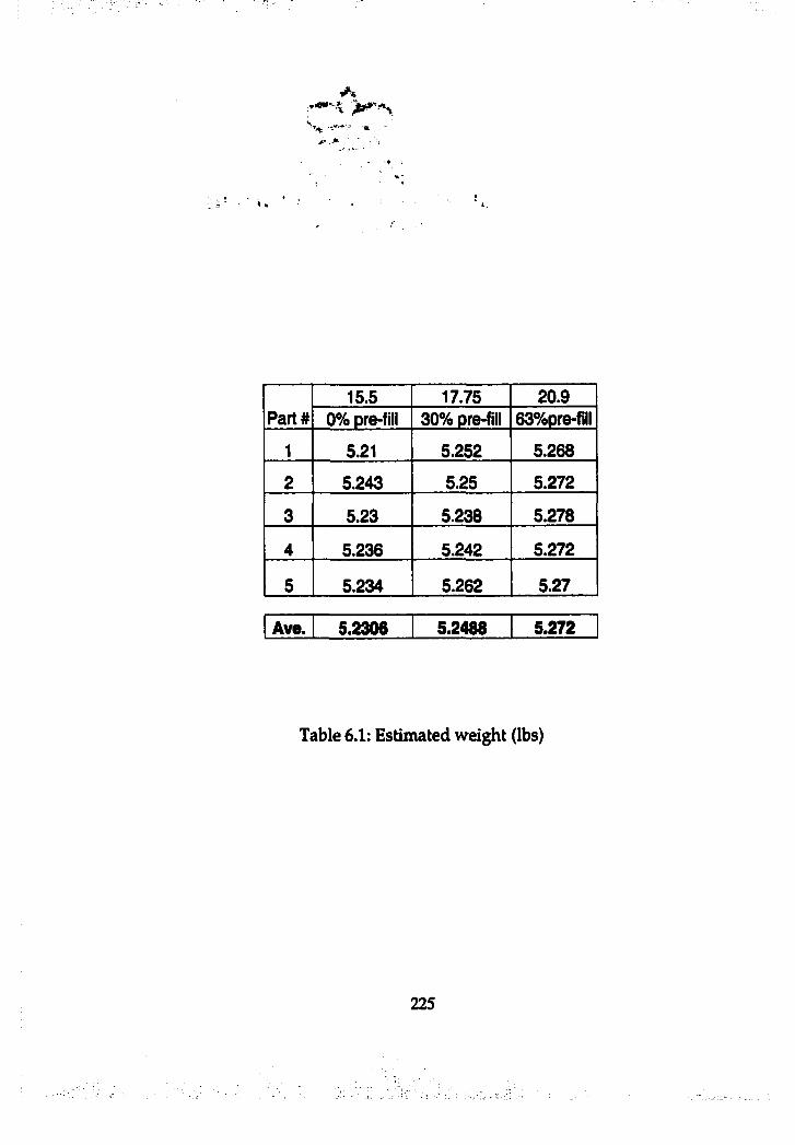
A*

P art#15.5 17.75 20.9

0% pre-fill 30% pre-fill 63%pre-fill

1 5.21 5.252 5.268

2 5.243 5.25 5.272

3 5.23 5.238 5.278

4 5.236 5.242 5.272

5 5.234 5.262 5.27

Ave. 5.2306 5.2488 5.272

Table 6.1: Estimated weight (lbs)

225

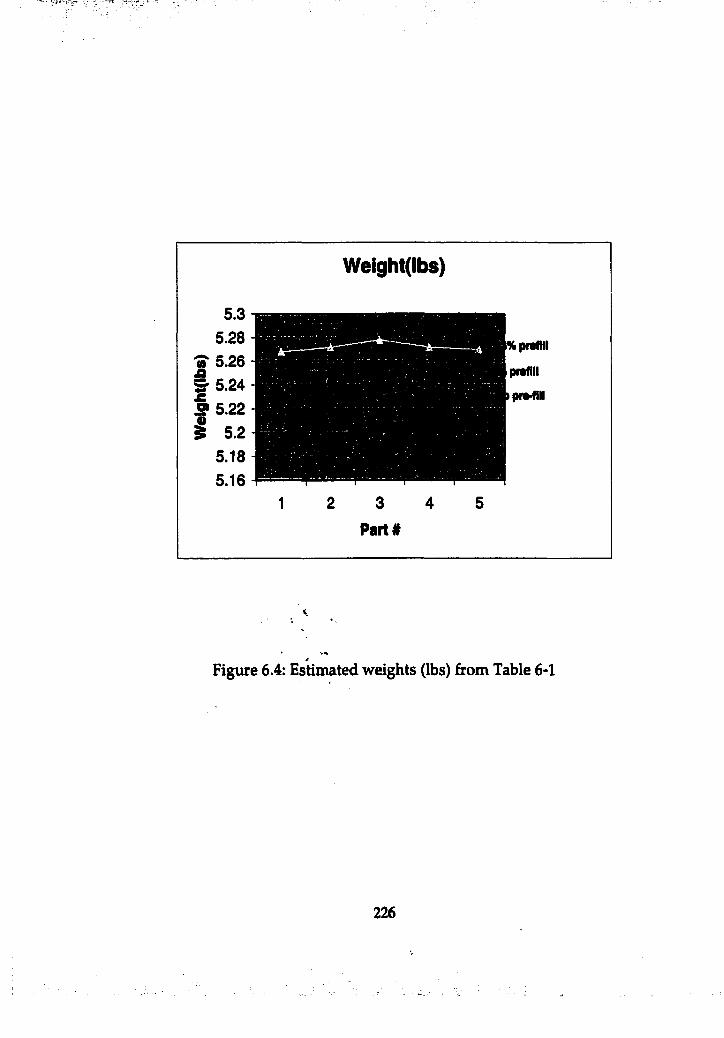
Weight(lbs)

s r 5.24S 5.22

Figure 6.4: Estimated weights (lbs) from Table 6-1

226

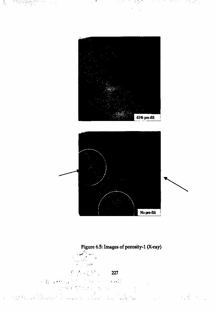
63% pre-fill

No pre-fill

Figure 6.5: Images of porosity-1 (X-ray)

227

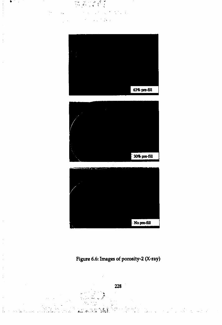
f f - -

63% pre-fill

30% pre-fill 1

Figure 6.6: Images of porosity-2 (X-ray)

228

As predicted/ significant pores were observed in the castings produced

using no pre-fill and 30 % cavity pre-fill, while no significant porosity was

found in the castings produced using 63% of cavity pre-fill (Figure 6.5,

Figure 6.6).

A large circled are in Figure 6.5 shows porosities generated in a

relatively thin section in the casting. It was clearly observed that those pores

created without pre-fill were significantly reduced using 63% of cavity pre­

fill. The pores observed in the thin section were considered to be gas

porosities generated by air entrapment based on shape of the pores and the

nature of the porosity generation. As mentioned earlier in Chapter 2,

shrinkage induced pores are created in relatively thick section of the

castings. In Figure 6.6, using cavity pre-fill, significantly reduced porosities

in another relatively thin area of casting are shown. Using 63% of cavity

pre-fill, pores were hardly observed as compared to using 30% and no pre­

fill.

However, it is not clear whether the gas porosity was all vanished or

distributed widely in the castings using high percentage cavity pre-fill.

Based on the radiographic results, following possible conclusions can be

drawn: 1) all air was vented using high percentage cavity pre-fill, 2) using

high percentage cavity pre-fill, trapped air was widely or uniformly

L A ' *r d r ' » . I » Ji . t ' v ' v ' ' I L i '■

distributed with much smaller diameters of voids in the castings, or 3) some

air was vented and trapped air was widely distributed.

To investigate whether the trapped air in the casings was vanished or

distributed with smaller diameters of voids, the castings were cut and

investigated with microscope (lOOx). The small voids were hardly observed

in the castings produced using 63% cavity .pre-fill. Thus, it would be

reasonable to conclude that most (not necessarily all) gas pores must be

reduced using cavity pre-fill, rather than distributed uniformly in the

castings.

In the above experiment, based on results of casting weight,

radiography, and microscopic investigations, it was found that gas porosity

associated with air entrapment was reduced using cavity pre-fill. Also, more

pre-fill employed, the less amount of gas pores created in the casting.

Regression model vs. Experimental results

The regression model (Equation 5.6) developed in previous chapter was

evaluated in a qualitative manner by comparing with the experimental

results. Casting geometry parameters were regarded as a middle value of

two coded levels except a parameter of Flow Disturbance (FD). The

parameter FD was set 1.0 as coded since estimated FD value was about 1.3,

230

. V- ». "■- .. ' V. A ?- * L.- •

. . . - - ' , ' - . ' i i ‘ : • - , i . - ' 4 " 4 / ■ ' i

which means that there is a certain degree of flow disturbance in the cavity

geometry or metal flow detours when it travels hom gates to vents in the

cavity. One of the injection parameters, cavity pre-fill velocity used in the

experiment was critical slow shot velocity. Figure 6.7 is the corresponding

contour plot of the regression model (transition time vs. cavity pre-fill).

231

-Iff**

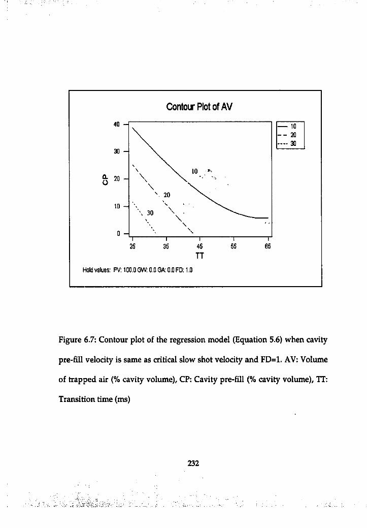
Contour Plot of AV

40 -

30 -

Q.ü

10 -

25 35 45 55 65TT

Hold values: PV: 100.0 GW: 0.0 GA: 0.0 FD: 1.0

- 10 — 20 30

Figure 6.7: Contour plot of the regression model (Equation 5.6) when cavity

pre-fill velocity is same as critical slow shot velocity and FD=1. AV: Volume

of trapped air (% cavity volume), CP: Cavity pre-fill (% cavity volume), TT:

Transition time (ms)

232

•r \ r *

The, aboYÇ contour plot predicts that more amount of cavity pre-fill

reduces more amount of air entrapment. Even though 63% of cavity pre-fill

is out of the range, in general, the trend of contour plot shows that 63% of

cavity pre-fill is better than 30% of pre-fill to reduce air entrapment when

employing cavity pre-fill. When transition time is short (less than 25 ms),

the trend of contour plot indicates that higher percentage of cavity pre-fill is

required to minimize air entrapment in the die cavity. Approximately, at 10

ms of transition time, 63% seems to be the required percentage cavity pre-fill

to reduce the amount of air entrapment to only 10% of cavity volume. In

fact, in experiment, about 70% of cavity pre-fill produced the best quality of

castings, which was almost porosity free.

Theoretically, the trend of the above contour plot (regression model)

indicates that more than 63% of cavity pre-fill may reduce more porosity in

the castings. To investigate that, about 80% of cavity pre-fill was tried.

However, the quality of castings produced using 80% of pre-fill was the

same as the quality of castings produced without pre-fill. The reason was

excessive time delay (early solidification of gate area) and the size of plunger

and length of shot sleeve. There was no enough room for the plunger to

travel in the shot sleeve to reach fast shot velocity.

233

Unfortunately, quantitative evaluation of regression model was not

completed since amount of trapped air was not measured In the experiment.

Besides, since selected percentage of cavity pre-fill and transition time were

out of ranges of the parameters In regression model, the trend of regression

model was evaluated qualitatively by comparing with experimental results.

However, the possibility that the regression model can be used to predict

optimum ranges of cavity pre-fill percentage based on the other parameters,

was shown.

234

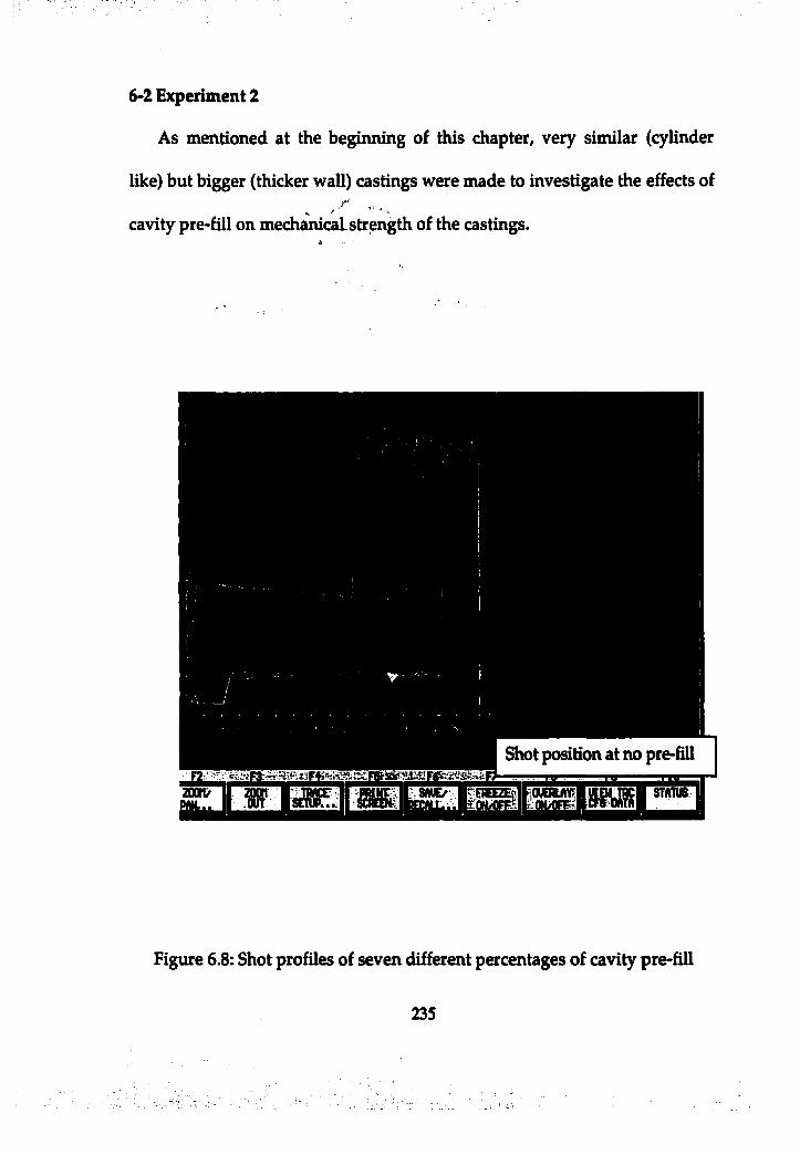
6-2 Experiment 2

As mentioned at the beginning of this chapter, very similar (cylinder

like) but bigger (thicker wall) castings were made to investigate the effects of

cavity pre-fill on mechanicaLstrength of the castings.

Shot position at no pre-fill

Figure 6.8: Shot profiles of seven different percentages of cavity pre-fill

235

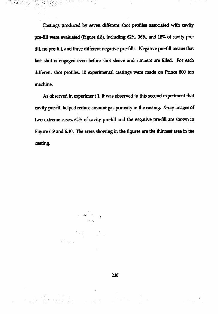
Castings produced by seven different shot profiles associated with cavi^

pre-fill were evaluated (Figure 6.8), including 62%, 36%, and 18% of cavity pre­

fill, no pre-fill, and three different negative pre-fills. Negative pre-fill means that

fast shot is engaged even before shot sleeve and runners are filled. For each

different shot profiles, 10 experimental castings were made on Prince 800 ton

machine.

As observed in experiment 1, it was observed in this second experiment that

cavity pre-fill helped reduce amount gas porosity in the casting. X-ray images of

two extreme cases, 62% of cavity pre-fill and the negative pre-fill are shown in

Figure 6.9 and 6.10. The areas showing in the figures are the thinnest area in the

casting.

236

.g

Figure 6.9: Images of X ray-3 (Castings produced using 62% of cavity pre-fill)

237

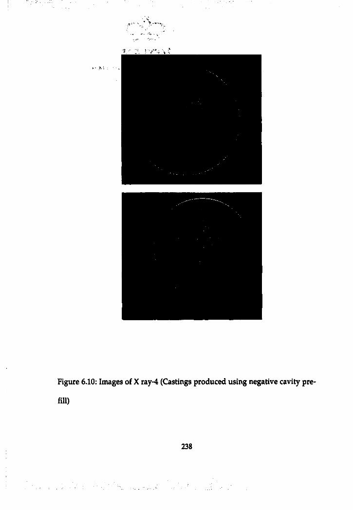
,.T-“

Figure 6.10: Images of X ray-4 (Castings produced using negative cavity pre­

fill)

2 3 8

^ '

Many pores were clefurly found in the castings produced using negative

pre-fill (Figure 6.10), while no pores were found in the thiimest section area

of the castings produced using 62% of cavity pre-fill (Figure 6.9). Since this

selected area is the thinnest section area, pores found in that area are

considered to be gas induced pores rather than shrinkage related.

In addition to the investigation of porosity distributions associated with

air entrapment, in this experiment, cavity pre-fill effect on mechanical

strength was investigated. This could be another indirect way to show,

quantitatively, the effects of cavity pre-fill on air entrapment and

accordingly gas porosity as the mechanical strength of the thinnest section

area was investigated. As mentioned in Chapter 2, porosity in the castings

makes significant difference in mechanical strength.

For the investigations, the maximum pressure that the castings of

cylinder can hold inside was measured (Table 6.2). Six castings were

randomly selected out of 10 castings produced for each different cavity pre-

M percentages and maximum pressure was measured. In Table 6.2, average

values are trimmed averages excluding highest and lowest values measured.

239

.

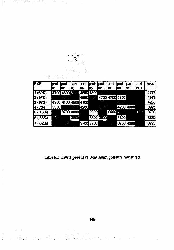
EXP. part part part part part part part part part#1 #2 #3 #4 #5 #6 #7 #8 #9

part#10

.l:-;(V) g M ER?][y^O]EW'I']k#&hL^##[^çl^k5[0]gkO][5[Oj -1' ____E R E M lE E S j] - : :%wol -i.v E J*lg[«i»!»]

^E O T J-uxk 'i E g g R g g E g g E g g ,

■IK)!: E g g E g g E g g g g g

Ave.

4775457542503925370038503775

Table 6.2: Cavity pre-fill vs. Maximum pressure measured

240

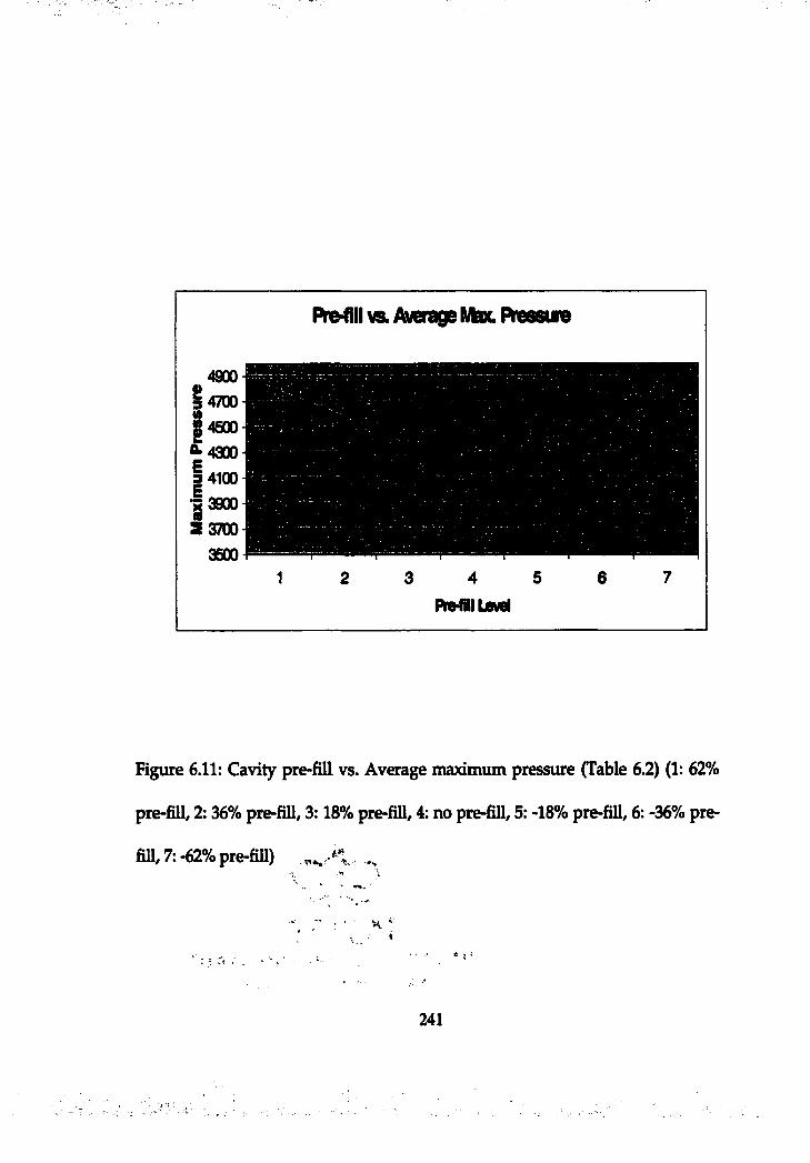
AeOII v& Average Max. Ressue

“•4300a 4100*5 39005 3700

Figure 6.11: Cavity pre-fill vs. Average maximum pressure (Table 6.2) (1: 62%

pre-fill, 2:36% pre-fill, 3:18% pre-fill, 4: no pre-fill, 5: -18% pre-fill, 6: -36% pre­

fill, 7:-62% pre-fill)

241

. .. i

- fe ■„■.As can be seen ïni F i^ ë* 6.11/ cavity pre-fill improved maximum pressure

that castings of cylinder can hold inside. The results show that the more

percentages of cavity pre-fill used/ the higher maximum pressure can be

achieved. The correlation between pre-fill percentages and maximum pressure

was almost linear when pre-fill was employed. However/ negative percentages

of pre-fill caused low and inconsistent maximum pressure. Since critical slow

shot velocity in the shot sleeve was not used due to early fast shot engagement,

unexpected air entrapment in the shot sleeve may increase amount of gas

porosity in the casting and the gas porosity may reduce mechanical strength.

Upon obtaining positive results of pre-fill effects on mechanical strength,

microstructures of castings were also investigated. Since microstructures of

castings are not uniform, burst areas by excessive pressure were selected and

investigated (Figure 6.12).

Different microstructures were observed using different percentages of

cavity pre-fill. This change of microstructure may influence mechanical strength

in addition to porosity contents in the castings. More silicon needles and coarse

structure as well as pores were found in castings produced without pre-fill or

negative pre-fill, which may cause stress concentrations.

hi this experiment, it was observed that there might be additional cavity pre­

fill effects on mechanical strength of castings hi addition to reducing gas porosity

contents in the castings.

242

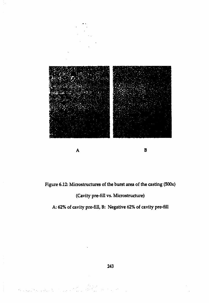
B

Figure 6.12: Microstructures of the burst area of the casting (500x)

(Cavity pre-fill vs. Microstructure)

A: 62% of cavity pre-fill, B: Negative 62% of cavity pre-fill

243

CHAPTER?

CONCLUSIONS AND FUTURE WORK

7.1 Conclusions

Conclusions were drawn out of the results of computer flow models,

regression model, and experimental castings. Thus, it should be noted that

there exist limitations of model applications as the models were developed

under the assumptions and experimental castings were conducted under the

limited conditions. The details of the limitations can be found in the related

chapters. In summary, the limitations are: 1) computer flow models were

assumed to be in adiabatic and isothermal condition, so that thermal effects

on flow patterns were ignored, 2) A regression model was developed using

the method developed under the assumptions to estimate amount of air

entrapment. The details of the method and its accuracy issues were

discussed and evaluated in Chapter 3.3.2,3) in the regression model, ranges

of selected parameters were limited. Also, there exist limitations of the

244

application of parameters, such as flow disturbance (FD) (Chapter 5.1), and

4) In experimental castings, there existed noises in shot profile control and

temperature control of die.

Conclusions drawn from this research are:

1) Cavity pre-fill changes filling patterns as it promotes lateral (or

unilateral) expansion of cavity flow. The lateral expansion of flow can

be a major benefit in some casting designs because it generates more

uniform cavity filling.

2) The uniform cavity filling helps reduce air entrapment, and

accordingly gas porosity in the castings as more molten metal is filled

before vents are covered.

3) Using cavity pre-fill, the reduced gas porosity helps increase

mechanical strength of castings.

4) Cavity geometry including gate and vent locations is the most

significant factor influencing air entrapment in the die cavity.

Percentage cavity pre-fill and transition time are also very important

injection factors to be controlled to reduce air entrapment when

employing cavity pre-fill approach.

5) To take advantage^^of the beneficial effect of cavity pre-fill, 1)

appropriate combihatibhs of injection parameters (e.g. transition time

I & <. . - 2 4 5 , I-5

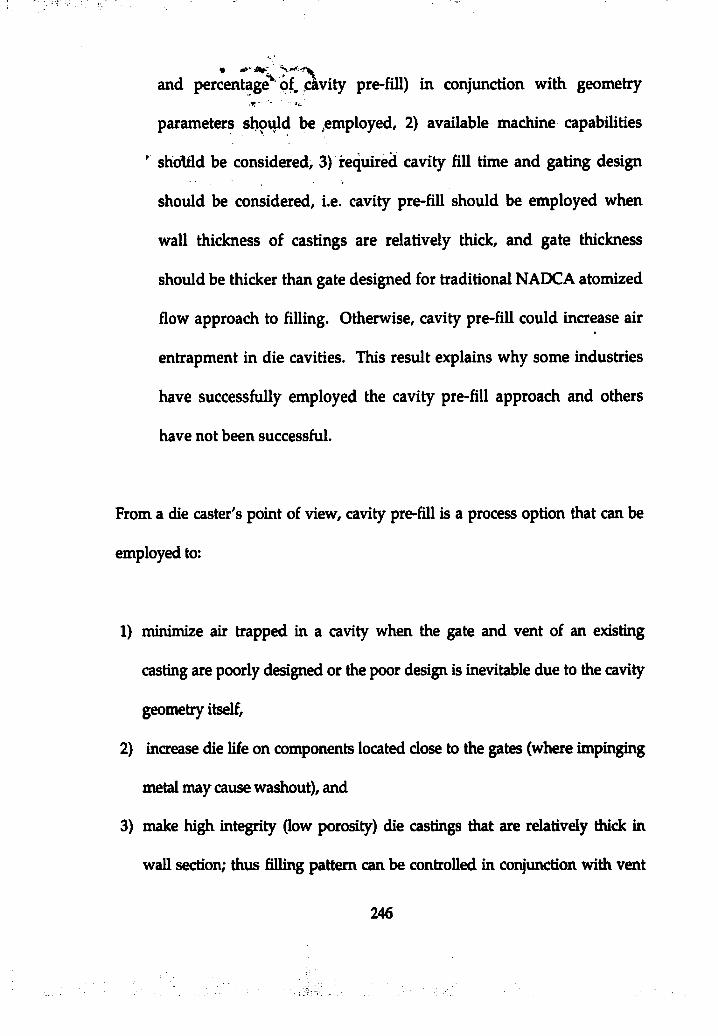
and percentage^ pf. cavity pre-fill) in conjunction with geometry

parameters should be employed, 2) available machine capabilities

shoWd be considered, 3) required cavity fill time and gating design

should be considered, i.e. cavity pre-fill should be employed when

wall thickness of castings are relatively thick, and gate thickness

should be thicker than gate designed for traditional NADCA atomized

flow approach to filling. Otherwise, cavity pre-fill could increase air

entrapment in die cavities. This result explains why some industries

have successfully employed the cavity pre-fill approach and others

have not been successful.

From a die caster's point of view, cavity pre-fill is a process option that can be

employed to:

1) minimize air trapped in a cavity when the gate and vent of an existing

casting are poorly designed or the poor design is inevitable due to the cavity

geometry itself,

2) increase die life on components located close to the gates (where impinging

metal may cause washout), and

3) make high integrity (low porosity) die castings that are relatively thick in

wall section; thus filling pattern can be controlled in conjunction with vent

246

placement/and thick gates can be used to feed solidification shrinkage

during intensification. %

The first option is a corrective measure that can be employed to improve the

quality of casting that has already been designed. The last two options

should be decided upon in the die and process design phase of engineering

in order for the casting to be successful.

Most die casters use critical slow shot velocity as a cavity pre-fill velocity

and most casting (cavity) geometry has a certain degree of flow disturbance

(i.e. FD is more than 1). Thus, in many cases, a contour plot of regression

model (Figure 6.7) will help die casters to determine optimum cavity pre-fill

percentages with their own transition time setup and constraints of machine

capability, and required fill time due to casting geometry and gate design

(Appendix J).

7.2 Future Work

1) In this research, only behavior of cavity flow and its effect on air

entrapment in the die cavity was investigated excluding thermal

effects of metal flow assuming adiabatic and isothermal condition.

Including thermal effects in the model, required cavity fill time

247

associated with casting geometry and required gate thickness in

conjunction with thè required cavity fill time are expected to be

assessed.

2) As mentioned earlier, due to delayed cavity fill time, cavity pre-fill is

effective when relatively thick walled castings, such as automotive

parts. Usually, automotive parts with thick walled section require

relatively high mechanical strength. Since microstructure changes in

the castings were observed employing cavity pre-fill in this research,

mechanical effects of cavity pre-fill in microstructure during delayed

filling and solidification are also expected to be investigated in the

near future. In addition to minimizing gas porosity (air entrapment),

microstructure changes might help enhance mechanical strength of

castings when employing cavity pre-fill.

248

Appendix A

Calculation of Gas Contents in Vacuum Fusion Test

249

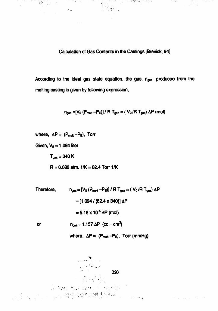
Calculation of Gas Contents In the Castings [Brevick, 94]

According to the Ideal gas state equation, the gas, ngas, produced from the

melting casting Is given by following expression,

ngas =[Vo (Pmelt-PE)] / R Tgas = { Vq/R Tgas) AP (mol)

where, AP= (Pmeit-PE), Torr

Given, Vo = 1.094 liter

Tgas = 340 K

R = 0.082 atm. 1/K = 62.4 Torr 1/K

Therefore, ngas ~ [Vo (Pmeit ~Pe)] / R Tgas ~ ( Vo/R Tgas) AP

= [1.094/(62.4 X 340)] AP

= 5.16x10^A P(m ol)

or ngas=1.157AP (cc = cm^)

where, AP= (Pmait-PE), Torr(mmHg)

250

Appendix B

Calculator for Estimation of Trapped Air Volume

251

CavitvVolume ■ . . . 14.0202 in cuCavitv Pre-fill 30 %Gate Area . ' • ' 0.146 in sqPrefill Gate Velocity 123.06 in/s

‘ w \ Cavity Pre-fill TimiÏFast Shot Gate Velocity 1500 in/sTransition Time 35 m s

prefi Urne Trans Une

Time when vents are sealed bm m m sM ms

V ents sealed during cavity pre-fill ? N 0 ,A n a . le a tp a n n e l2 |Volume filled when vents are sealed Go To N ext P a n e l incu

EWmatmd E nW nedA lryblw m *T uT h* |W ^^ In c u

Vents sealed even before A st shot starts ? NO 1

Volume filled when vents are sealed 11.79419151 incu

E M i n a t i d ^ i l n ^ ^ p 2 2 2 6 0 9 B ^ . In c u

w

252

Appendix C

Planning for Numerical Experiment

253

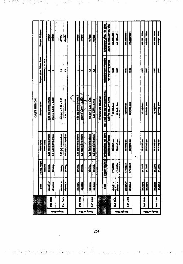
I

I

I!l

I

i

I

I I

I I

!

I InE S

1 1

i

•nd«id<<w

I I

i f

I I

IÎ

lU

Î 1

lit fi l l

II

II

i

f

I I

II

I I

i

I I

II

i l

I I

I I

I I

e e

I I

254

Appendix D

Array of Design of Experiment

. 255

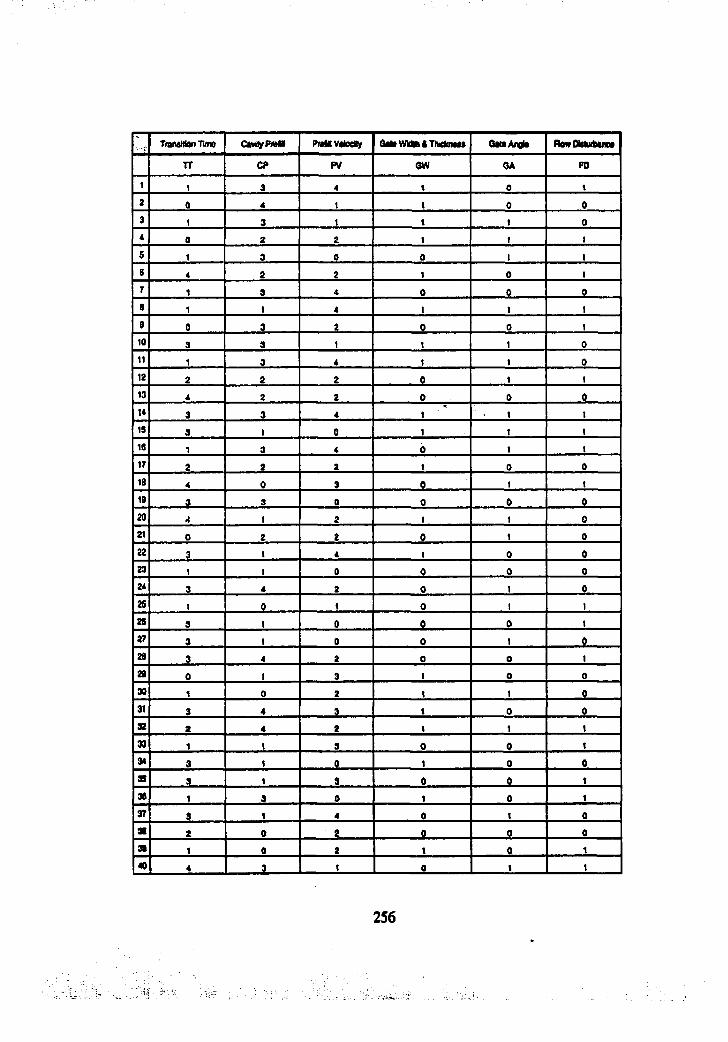
TraMMonTiino CtMiyPmlB Pn«5V4lacl7 OiHVMiGKlThidowM OMAngl* FtawOittHblim

TT CP PV 6W <3A FD

1 1 3 4 1 0 t2 0 4 1 1 0 03 1 3 1 1 1 04 a 2 2 1 1 1

5 1 3 0 0 1 1

B 4 2 2 1 0 1

7 1 3 4 0 0 0B 1 1 4 1 1 1

9 0 3 * 0 0 110 3 3 1 1 1 0

11 1 3 4 I 1 0

12 2 2 2 0 1 1

13 4 2 2 0 0 014 3 3 4 1 • 1 115 3 1 0 1 1 1

15 1 3 4 0 1 1

17 2 2 2 1 0 0

18 4 0 3 0 1 t

19 3 3 0 0 0 0

20 4 1 2 1 1 021 0 2 2 0 1 0

22 3 1 4 1 0 023 1 1 0 0 0 024 3 4 2 0 1 0

25 1 0 1 0 1 1

25 3 1 0 0 0 1

27 3 1 G 0 t 0

28 3 4 2 0 0 1

29 0 1 3 1 0 0

30 1 0 2 1 1 031 3 4 3 1 0 032 2 4 2 1 1 1

33 1 1 3 0 0 1

94 3 1 0 1 0 0

35 3 I 3 0 0 1

38 1 3 0 1 0 1

37 3 1 4 0 1 0

35 2 0 z 0 0 0

35 1 0 2 1 0 1

40 4 3 ■1 0 1 1

256

Appendix E

Calculations for Numerical Experiment

257

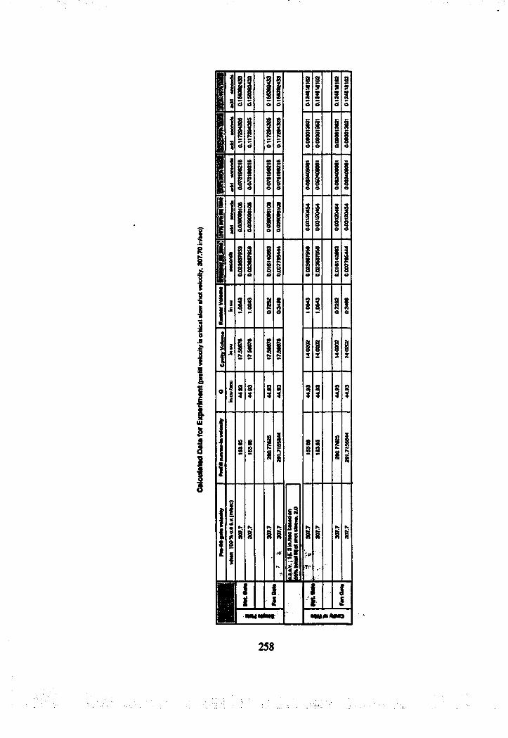
I

I

lUsII

I

I

I I

i ;

I I

i t

258

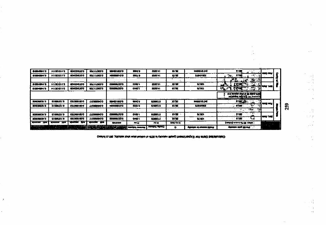
«WMMno Tuseiouti aotcouoo toinmaro wtEgtwra ■Mro amr»i OlfC MOMICiK•MNMM‘0 HltBIOll'O tottœjtto auituon emo «MOPI •>« J

f■ f ..rC. ^ t«iwmtfo «IISEWU-0 mmfum soiiuaaro asaauan» ■MOI a»r»t UIKI isMmm-0 tiiseioUD matum mutuauro TWWMfTWO CMori aaa>i cm U«l -

tgOKMMtO «SUMIE0O utmuao «MtMOirO ■nro tmni :om MtntrtfcnSCMCM'O EtfMtti'O GU(Mt«00 ittunmro sera UMF/I cm CMIfOK 17 .:■ %, rf 190S(«KSi‘0 ««HtCt'D CEUMMTO iismmurù EEWQtfWIfO CMOI «aoTii •*« «Wt . . . . . . . . . . . . . . . . . . . . . . . .m V 1QOWfO CtSHiSi'D CBlaMMoa itfNtOMV «0S8MUdr6 CMOl tttorxi «m U-Ott - % cm w 'tçuaam pp» •PUOOM ppc •PWOW PPP (puoap# rai» aacrmui <3»WW3%a,*#; ■■Bi■HBÉÉ■■■■I mmÊÊisstÊBsmBÉÉBti —nonuumg 1 —1** *wa O gnMiiimwimiiw ■ ■ H

s

(NiVUI S * IK ‘A«ao|M tog t «M|t |«(IM910 « S 8 •) A im im wMd) IIMIIIIJMixa MU u s a po iim aiio

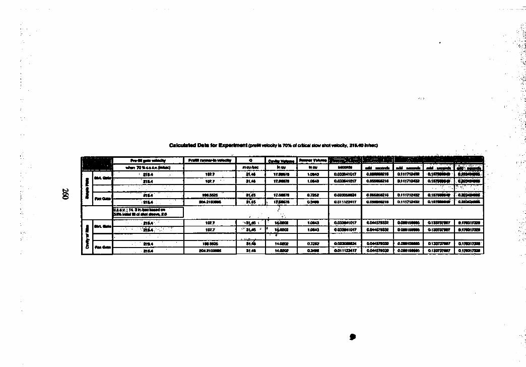
CalcuMwf Oala for Expwimant dwelM «•todDT is 70» <4 crittcal (low atM wMocky. 21&40 kw!M4

■ ■ B I ■Hiiiiwwrar mio iwBwt* wuear 0 BWiiiiilia ■s Hb t m m m m m■■N 14m 70%c»MMOmtft inwaec fcicu Mcu 6400801 add 440*6181M IW.? 31.46 1748678 14843 0433841017 0486868018 0111712432 0107888048 'W88438388.:

i aM,OMB ■'liM W .7 31.46 1748678 14848 0433641017 0488686016 0111713430 01678888 W ,''0 # 4 2 # 8 8 -

f# ai64 IMXS29 8148 1746878 47360 0403086634 0468866316 0111712432 01678888# ; 0.303131888

r w o M' ■ ; « M : aotxioaMa 31,45 , , 1746678 0.9488 0411122417 0.068868016 0111712482 01878886# 0771411801

e*»M ; ? * S h w e » w » w SSKiiiMM ■ el «M a iM , 1

W M IW.7 '3L45 \ 144800 14648 0433841017 0444579330 0086188885 0133737887 0178317338

i aMOM*107.7 3145 f ‘ 144000 14843 0433841017 0044578330 0088188885 0183737887 01783173#

« “ •“ T

Î naOM a ■ ■ «18.4 •888638 S lA 144000 0.7280 0003086031 0044578930 0088188688 0133737887 01783173#«1*4 8042100886 31.45 144000 04488 0411122417 0044578330 0486186865 0133737887 01783179#

I

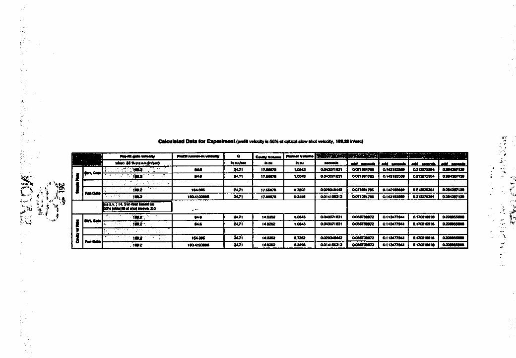
Celculetsd Deta lo r ExperSment (pieHI vwloc*y is 65% d critical slow shot veloo«y, inAe<4

i j ift. I

Im iw o w w * W W W a CnWVMMW W— IIV W H E B E B H U aS f m S a d W

add aacaadi

■ 4

MPP nhm incu Awe la DU mou aw oadt

I1

Ê4M « J 1 17JW7B 18048 0843071031 0871*1700 01481033* 0813873334 08043371*M 6 »».71 178M78 18043 084307103* 0 8 7 1 * 1 7 * 01481033* 0813873334 08043071*

" M w ; 1SC3M 84,71 I78M 18 07808 0080340448 0.071*17* 01481033* 0810870304 08043071*

- i # a ' 84,71 178*7# 0 8 4 * 0814100818 0 0 7 1 * 1 7 * 01481083* 0218870304 08043071*

W *v .; K S In M w b w d sn

.'.T

i1

Î

' 1 # g \ #4# 84.71 14.0102 *8043 0043071031 0*0730078 0113477044 01708100*0 0770 * 8 0 *•H

. w . % M jS 84.71 140808 1.0043 0.043071031 0*0730073 01134770*4 0 1 7 * 1 * 1 0 0 3 * 0 3 6 0 *

im » IW 9W 84.71 *40202 0.7808 0880340448 0000730873 0113477044 0170810010 0 88* 3 3 * 3

1«M IMl4«0SIW 84.71 140808 0 3 4 * 0814*008*8 0*0730078 01*3477044 017081*10 08800360* 4.i

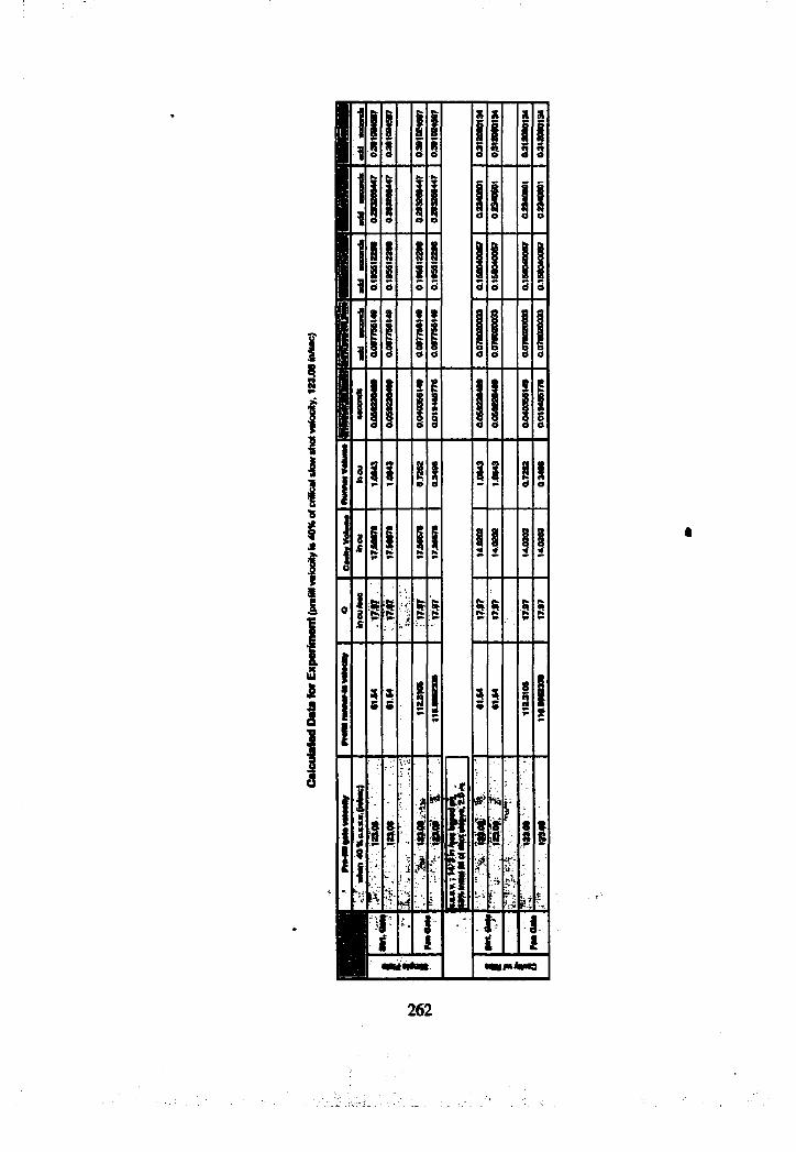
II%ij*

I I

I

■J

4-

i f

■À

mmmivaa

262

Appendix F

Estimated Responses

263

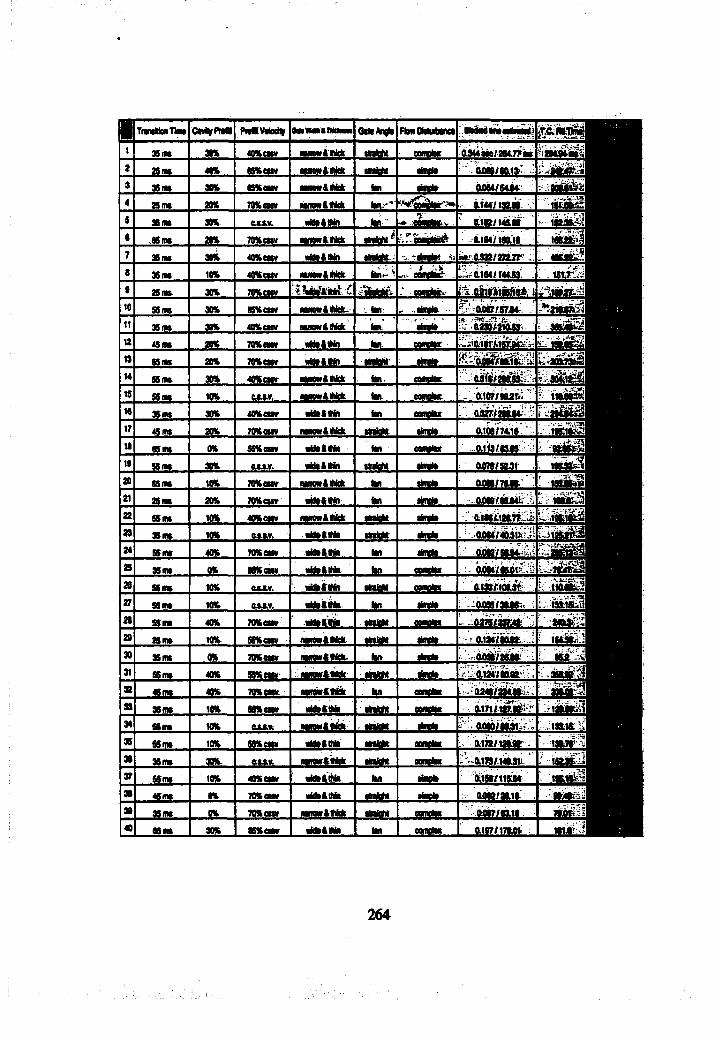
I T im M onT lM P itav iio cH y o u u u a o u u u G auao gl» F tanO tah a tanu ; ; o | a i a a a i i * d i ^ rn m M1 3 3 m t 30% 40% cam MWDwétlICk aM oM e o o am t o a u t é b / m n i i2 23 m 40% 83% «4W aim w fta iiek a im a it tam ia O ioâo/aoL isl : r : . # #3 3 8 m 30% 83% OU* « am » & 9 ih k tan ta m i» 0 0 8 4 7 6 4 0 4 r .Ü 2 Ô É m i4 2 3 m 20% 70% e u * lianw tiO iick im r ' ^ ^ a i ^ S u t a r » . 0 1 4471 3283 / i s a m ÊS 3 8 m 30% exM . « o u& o an taii ' -»:;{MBtalt>w .

c- . -0 1 8 2 7 1 4 9 8 8 >' l o ô M a

< .33 m 20% 70% CUV larm rS fiic fc . u a W a ^ 0 1 9471 8018 : I 8 Ë # #7 3 8 m 30% 40% e u * •M aS O U * M e « e . - 'ïtamtaat 4, U » 03 3272 7077 ^ . 4 8 2 m 28 3 6 m 10% 40% c u * M nooO aikfc eu tah iA - b L 01 8477 4433 : : i S l i Æ9 2 S m 30% 70% e u * i ’SÊÊUè. c o a d ta t, ' 0 Ô i 9 » i K A a à 1 ^-% 18027La10 3 3 m 30% 89% e u * ■. tan- , a h u le

ç r , - : - T - 't - 0 0 0 7 7 3 7 U r % 2 i ô W |

11 3 3 m 30% 40% e u * u m m S a U k tan " ' e t a d a ' • - t ' . o a o M o i s ô : : - # #12 4 S m 20% 70% e u * •M tâ O in tan e a a d a r jü W l'taT Â Î& 9 4% %13 3 5 m 20% 70% e u * W 99 89U aaataw- a ta d o14 3 3 m 30% 40% e u » « W S I i W t tan eoaaaac13 3 8 m 10% e*».* . M M w S aiIck tan e u a a u O l 0 7 7 9 8 2 f c ' r t i o i î SIS 3 3 m 30% 40% e u * M iU SM n tan C M d a t ■ 0N 7728Ô 84;i.%17 4 3 m 20% 70% e u * M itow S aaek aaataht a b q u O t0 8 7 7 4 il8 •19 a s m 0% a s % e u * « m a o i n tan c a a d K 0113783.88 t - : 8 0 8 ^19 a s m 30% tXM . « u a t o a n a ta W l ta m U 0 0 7 0 7 3 2 3 720 a s m 10% 70% e u * n a im tia iiD k tan a b n t t 00 8877 888 .: ’ -21 2 3 m 20% 70% e u * i# 9# lM m tan alm da O û887É 9i& :':? i22 a s m 10% 40% e u * « a n w a a ik k a u ta n t ta n d a / : 'O I 8 8 X l9 0 7 7 l l i :23 3 8 m 10% CM .». iriU O O Éi aaataht ahaola . " ..O 0 W 7 4 O 3 t'i‘J i34 a s m 40% 70% e u » w u a o a m tan ta n d a : ' 0 0 8 2 7 3 8 8 4 :.:23 3 3 m 0% 88% O M « M # & 3 # tan «m ata» o o o o f W i f . ; ü : 7 ^23 3 3 m 10% o u . * . W 9» 838 l aaataht m m 0 l # l d 0 3 7 i ; '

27 a s m 10% e u . » . « M a m W tan tam ia :O 088 /3O 88 h .28 a s m 40% 70% e u » ■ .'Wdoo'oii» aaataht m m L -:0 2 7 8 7 2 3 M 0 ■ i - d o i à i ^ i29 2 9 m 10% 96% e u * im m A 3 3 c% aaataht tanaaa 0 1 2 4 7 8 0 8 0 .30 3 3 m 0% 70% e u * im w a a i ie k . tan tam U omiaÙÊ : ' '8 0 2 " '- ^31 S 3 m 40% 3 8 % eu» M u u & a i iu aaataht a ta d a :/.% -.OI24'7809Ô '\:L32 4 S m 40% 70% e u * i w m r t a a â t t a » canetan . ' . - M i w i t j â i f e : ' ;33 3 8 m 10% 3 8 % e * u « u » c « a h aaataht m m34 36 m 10% e u * . « a m » * # # : . -a a a tah t tam ia ^ 0 0 8 i i 7 8 Ù l I ; / .33 a s m 10% ae% e * u aW aSO U aaataht eam ta* 0 1 7 2 /Ü a i u38 3 S m 30% e u » . aanew ClN ck aaataht o o n d n . 01 737 M031L37 a s m 10% 40%C*U « M ià 'M n tan tam ta 01 3 8 7 1 1 3 8 4 - ' I 8 0 # |38 4 S m 0% 70% e a u «M aA tM t a a m h t a ta d a 0 0 8 2 7 2 0 1 8 : -oodïO38 a s m 0% 70% e a u nanw rS taefc aaataht eam ta* 0 0 0 7 7 8 9 1 8 T M Ï i i40 8 3 m 30% 33% e a u U U tO É i tan c o n d K - 01 87717001 1810?

264

Appendix

Maximum Allowable Cavity Fill Time Calculator

2 6 5

»

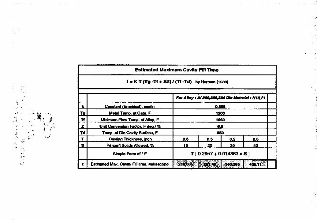
j " ■»,/

Estimated Maximum Cavity Fill Time

t ■ K T (Tg-Tf + SZ)/(Tf-Td) by Herman (1988)

ForAHoy : A !3 6 0 .3 8 0 ^ Of# M atartat : H13,21

k Constant (Empirical), sec/in 0.866

Tfl Metal Temp, at Gate. F 1200Tf Minimum Flow Temp, of Alloy. F 1060Z Unit Conversion Factor. F deg / % 6J3Td Temp, of Die Cavity Surface. F 650T Casting Thickness, inch 0.5 0.5 0.5 0.58 Percent Solids Allowed. % 10 20 30 40

Simple Form of *r T [ 0.2957 + 0.014363 x S ]

t Estimated Max. Cavity Fill time, mMisecond

Appendix H

Estimated Cavity Fill Time

267

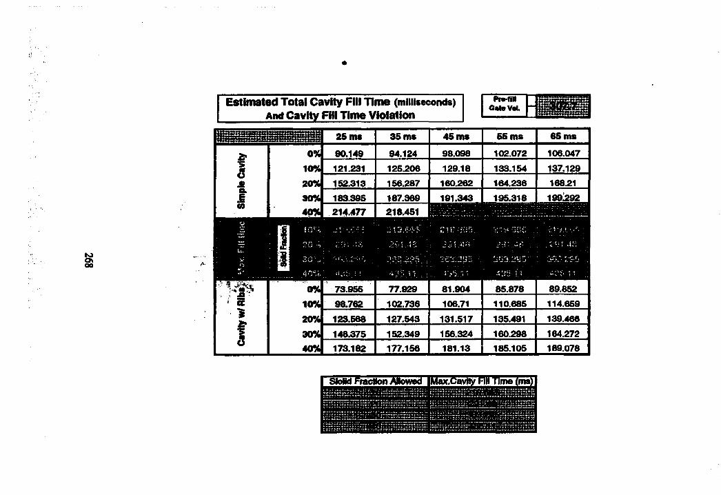
Estimated Total Cavity Fill Time (milliseconds) ________ A nd Cavity Fill Time Violation______

2» 0%

25 ms

90.149

35 ms

94.124

45 m s

98.098

55 ms

102.072

65 ms

106.047

1 10% 121.231 125.206 129.18 133.154 137.129

20% 152.313 156.287 160.262 164.236 168.21

M 30% 183.395 187.369 191.343 195.318 199^292*e

40% 214477 215.451

10% 73.9i56 77.929 81.904 85.878 89.852

10% 98.762 102.736 106.71 110.685 114.659

20% 123.568 127.543 131.517 135,491 139.466

f 30% 148.375 152.349 156.324 160.298 164.272o

40% 173,182 177.158 181.13 185.105 189.078

SloNdFmcMonAMwed IMax CavNy FIN Time (ms

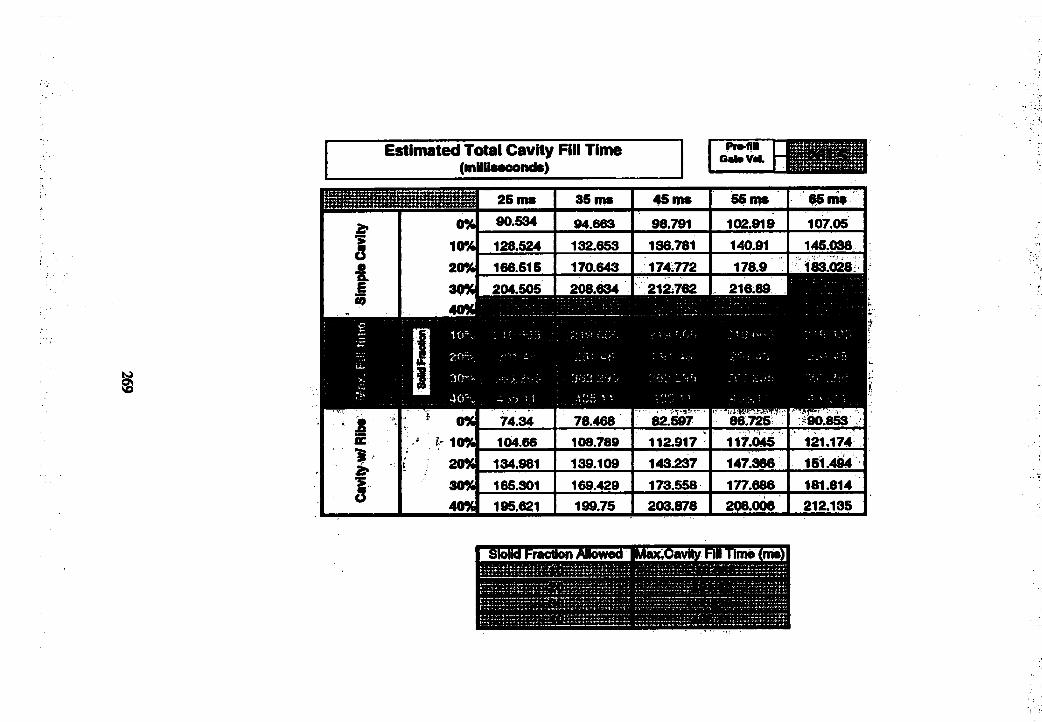
Estimated Total Cavity Fill Time (millsacondc)

P r» f i lGatoVaL

2* 0%

25 ms 90.534

35 ms

94.663

45 ms

96.79155 ms

102.919^ m s107.05

I 10% 128.524 132.653 136.761 140.91 145.036o4 20% 166.515 170.643 174772 176.9

M 30% 204jM5 206.634 ^ ^ 2 i e s ^w

40% fmBBÊtlKÊlM

§

0% 74.34 76.466 62.597 66;725 90 65310% 104.66 108.769 112.917 117.045 121.17420% 134.961 139.109 143.237 147.366 15l.4iM30% 165.301 169.429 173.556 177.666 161.61440% 195.621 199.75 203.876 206.006 212.135

Slolid Fraction ANowed

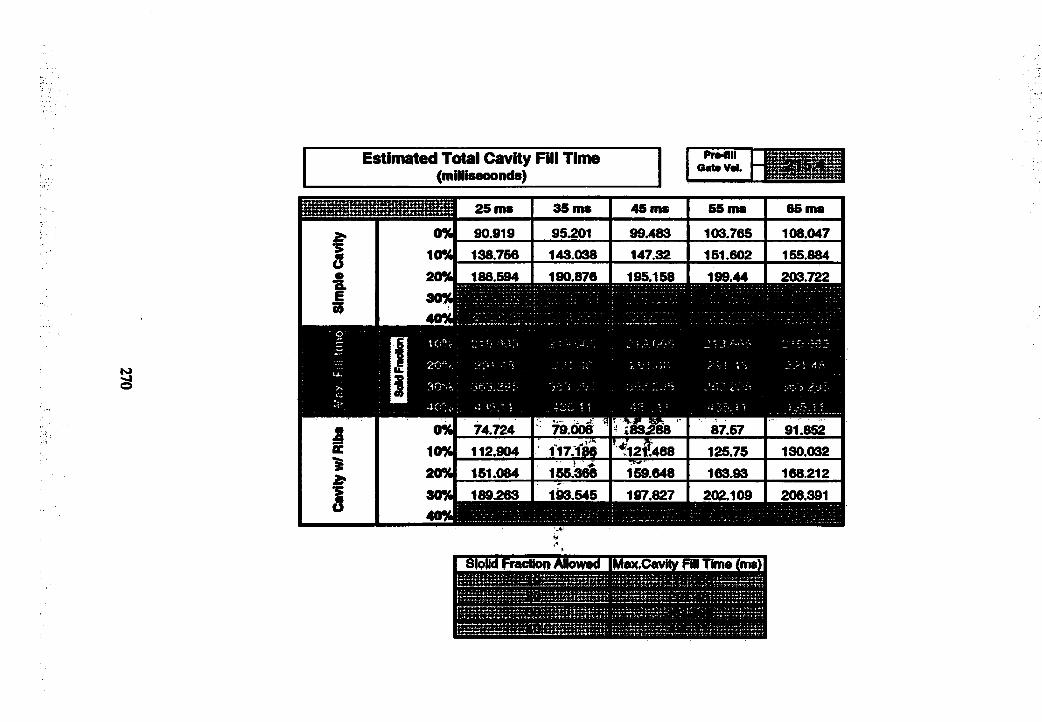
Estimated Total Cavity Fill Time(m illiseoonds)

35 ms25 ms 45 ms 55 ms 65 ms

95.201 99.483 103.765 108.04790.919138.756 143.038 147.32 151.602 155.884186.594 190.876 195.158 199.44 203.722

74.724 79.006 87.57 91.852112.904 11711B8 ’^12l1[4e8 125.75 130.032151.084 1 5 5 .^ 159.648 163.93 168.212189.263 1^ .545 197.827 202.109 206.391

Siplld Fmdkm Alkwvsd |Msx.C«vity Fn Time (ms

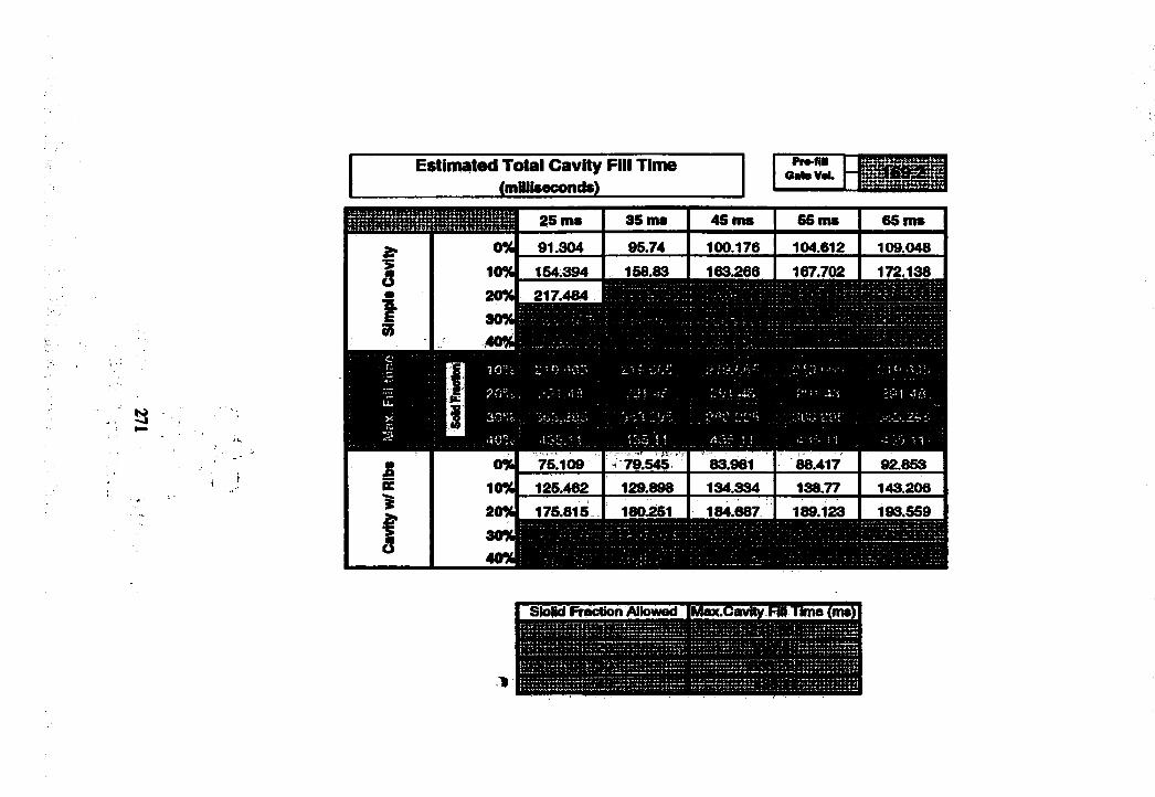
Estimated Total Cavity Fill Time (millisecond#) m a

35 m# 45 m s 55 ms 65 m s25 ms

95.7491.304 100.176 104.612 109.048158.83 167.702 172.138154.394

217.484

O Ê

5 0%S 10%a 20%

S 30%40%

75109. • -» r i ' f - X '’

79.545 83.961 M.417 92.853125.462 129.898 134.334 138.77 143.206175.816 180.251 184.687 189.123 193.559

SloHd FraotiQn Allowed

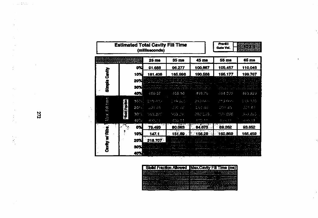
s

Estimated Total Cavity Fill Time(m illiseconds)

PW4IIG alaV al. ■ ;!î.îTJTmrHEtSî

:iîiî;i i-hiïmxiüîi2

218.707

25 ms 35 m s 48 m* 55 ms 65 ms

91.688 98.277 100.867 105.457 110.046181.408 185.098 190.588 195.177 199.767

.155.1 G 459.7^

:.T

160.860

8IpM Fraction Alowed

Appendix I

Coefficient of Regression Model and Significance of Factors

273

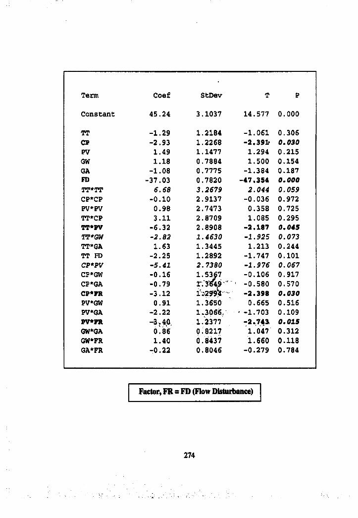
Term Coef StDev T P

C onscan t 4 5 .2 4 3 .1037 14 .577 0 .0 0 0

TT -1 .2 9 1 .2184 - 1 .0 6 1 0 .3 0 6CP -2 .9 3 1 .2268 -2 .3 9 1 / 0 ,0 3 0PV 1 .4 9 1.1477 1 .2 9 4 0 .215GW 1 .1 8 0 .7884 1 .5 0 0 0 .154GA - 1 .0 8 0.7775 - 1 .3 8 4 0 .187FD -3 7 .0 3 0 .7820 - 4 7 .3 5 4 0 ,0 0 0TT*TT 6.68 3.2679 2.044 0.059CP*CP -0 .1 0 2 .9137 - 0 .0 3 6 0 .972PV*PV 0 .9 8 2.7473 0 .358 0 .725TT*CP 3 .1 1 2 .8709 1 .085 0 .2 9 5TT*PV -6 .3 2 2 .8908 - 2 .1 8 7 0 .0 4 5TT*GW -2 .8 2 I .4630 -1 .9 2 5 0.073TT*6A 1 .63 1 .3445 1 .213 0 .2 4 4TT FD -2 .2 5 1 .2892 -1 .7 4 7 0 .1 0 1CP*PV - 5 .4 1 2.7380 -1 .9 7 6 0 .067CP*GW -0 .1 6 1 .5367 - 0 .1 0 6 0 .917CP*GA -0 .7 9 -0 .5 8 0 0 .570CP*FR -3 .1 2 f^Z994 ' - 2 .3 9 8 0 ,0 3 0PV*GW 0 .9 1 1 .3650 0 .665 0 .5 1 6PV*GA - 2 .2 2 1.3066 , ' - 1 . 7 0 3 0 .109PV*PR -3 ,4 0 , 1 .2377 - 2 . 7 4 1 0 ,0 1 5GW*GA 0 .8 6 0.8217 1 .047 0 .3 1 2GW*PR 1 .4 0 0.8437 1 .6 6 0 0 .1 1 8GA*FR - 0 .2 2 0 .8046 - 0 .2 7 9 0 .7 8 4

Factor, FR=FD (Flow Disturbance)

274

Appendix J

TT-CP Contour Plot of Regression Model

Cavity Geometry Effect on Air Entrapment (AV)

Cavity Pre-fill Velocity: Critical Slow Shot Velocity

Gate Angle and Rate of Gate Thickness and Width to

Total Casting: Middle Value

275

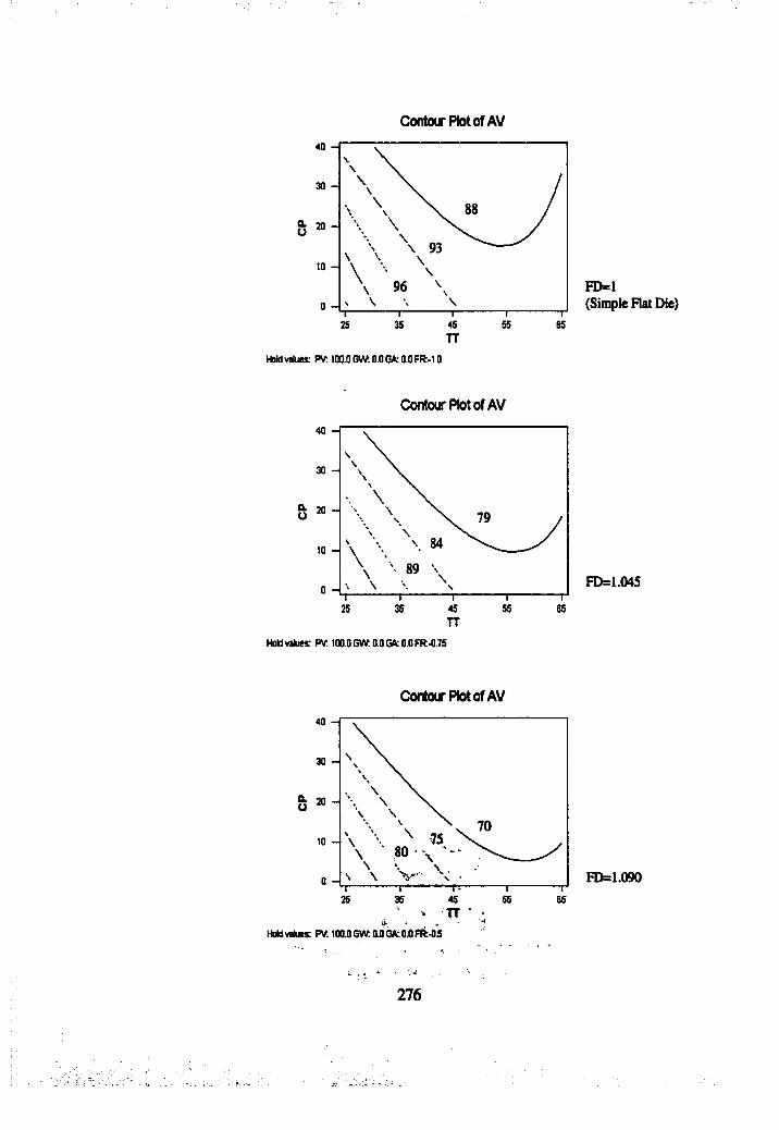
Contour Plot of AV

40

30

20

toFD=l(Simple Flat Die)0

25 35 45 55 65TT

Hold values; FV 100.0 GWI 0.0 G k 0.0 FR-t O

Contour Plot Of AV

u

TTHold values: PV: 100.0 GW. 0.0 GA; 0.0 FR-0.75

Contour Plot Of AV

TT ■

40

30

20

10

0

45 55 8525 35

40

30

20

10 - \

0

25 35 45 55

FD=1.045

FD=1.090

Hold values: PV1100.0 GWIHOGAzODFR^If

276

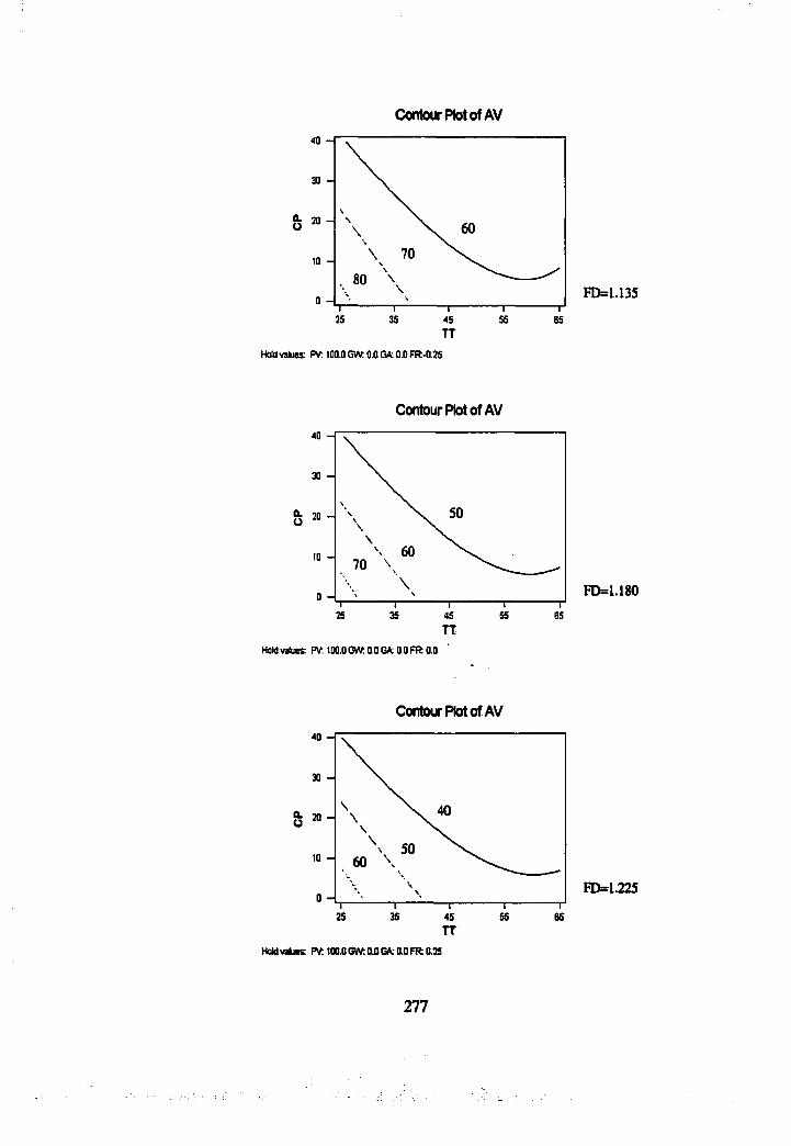
Contour Plot of AV

40

30

30

10

035 35 45 55 65

TTHaldvalues FV 100.0 GW; 0.0 GA: 0.0 FR-0.35

Contour Plot of AV

TTHold values: FV 100.0 GW 0.0 GA: 0.0 FR 0.0

Contour Plot Of AV

TT

FD=1.135

40

30

30

10

035 35 5545 85

FD=l.l80

40

30

30

10

0

35 35 55 6545

FD=1.225

HoM values: FV 100.0 GW OO GA: 0.01% 005

277

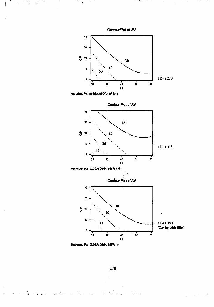
Contour Plot of AV

40

30

30

to

0

25 35 45 55 85TT

Hold values PV: 100.0 GW: 0.0 GA: 0.0 FR 0.5

Contour Plot Of AV

TTHold values PV: 100.0 GW 0.0 6A: 0.0 FR 0.75

Contour Plot Of AV

TT

FD=1.270

40

30

30

10

0

35 35 45 55 85

FD=l.3l5

40

30

10

08535 35 45 55

FD=1.360 (Cavity witli Rit»)

Holdvakics PV: lOOOGWIOOSkOaFR 1.0

278

LIST OF REFERENCES

[Alien, 00]: Allen, T. T., L. Yu, "The expected integrated mean square error criterion". Research report in the department of Lidustrial, Welding and Systems Engineering at The Ohio State University, Columbus, OH.

[ADCI, 77]: "An introduction to die casting", American Die Casting Institute, Des Plaines, IL, 1977.

[Apelian, '97]: Apelian, D., http://itri.loyola.edu/casting. 1997.

[Armentrout, '93]: Armentrout, D.J., "Investigation of the slow shot phase to minimize entrapped air in cold chamber d i^ fc tin g " , MS Thesis, The Ohio State University. ^

' V .

[Barkhudarov, '93]: Barkhudarov, M., et al., "Experimental validation and development of Flow-3D for casting problems". Modeling of casting, welding and advanced solidification processes VI, pp. 421-434,1993.

[Bar-Meir, '94]: Bar-Meir, G., Wrinkle, L., "Accurate PQ^ calculations ". Die casting engineer, pp. 26-30, N ov./ Dec. 1994.

[Bar-Meir, "98]: Bar-Meir, G., "How to calculate the PQ^ diagram". Die casting engineer, pp. 81-83, May/Jime, 1998.

[Barone, ’99]: Barone, M. R., D.A. Caulk, "A new method for analyzing cavity fill in die casting", NADCA Transactions, paper No. T99-013, pp. 15-22,1999.

279

[Bartling, '66]: Bartling, L. A., "Recent improvements in instrumentation for study and control of die casting variables". The fourth national die casting exposition & congress, paper No. 1303, Nov. 1966.

[Bennet, '61]: Bennet, F. C., "Gating magnesium die castings". Foundry, pp.104-107, Nov. 1961 and pp. 75-79, Dec. 1961.

[Bennet, '66]: Bennet, F. C., "Designing die casting dies to work on early shots". The fourth national die casting exposition & congress, paper No. 503, Nov. 1966.

[Box, 59]: Box, G. E. P., Draper, N. R., "A Basis for the Selection of a Response Surface Design." Journal of American Statistics Association, Vol. 54, pp. 622-654. 1959.

[Brevick, '94]: Brevick, J. R., Z. Israel, S-H. Cheng, Y-L. Chu, B-S. Chun, "Vacuum assisted die casting: casting properties and contained gas contents", ERC/NSM Report, No. C-94-52, The Ohio State University, Columbus, 1994.

[Brevick, '99]: Brevick, J. R., C. Mobley, "An evaluation of defect occurrence and causes in die cast aluminum alloy transmission cases". Final Report, The Ohio State University, Columbus, 1999.

[Chen, 91]: Chen, S., et al., "Simulated filling of dies with cores", NADCA Transactions-T91-093,1991.

[Cheng, ’95]: Cheng, P., J. R. Brevick, "Squeeze casting process and fatigue behavior of squeeze cast A380.0 alloy", ERC/NSM Report, No. C-95-35, The Ohio State University, Columbus, 1995.

[Davis, ’85]: Davis, A. J., S. J. Asquidi, "Water analogue studies of fluid flow in the die casting process", SDCE 13th international die casting congress and exposition. Paper No. G-T85-063,1985.

280

[DePorto, 72J: DePorto, R. G., J. F. Wallace, "Effects of type of jet flow in filling die on optimum fill time". Die Casting Research Foundation Report, Nov. 1972.

[Dinehart, 98]: Dinehart, A., Personal conversation, Visi-Trak corporation.

[Domanus, '86]: Domanus, H. M., et al., "Fluid flow and heat transfer modeling for castings". Proceedings of the third conference on modeling and control of casting and welding processes, Jan. 1986.

[Duran, '91]: Duran, M., "Minimization of air entrapment in the shot sleeve of die casting machine to reduce porosity", MS Thesis, The Ohio State University, 1991.

[Eady, '86]: Eady, J.A. and Smith, D. M., "The effect of porosity on the tensile properties of aluminum castings". Materials Forum, Vol. 9., No 4,1986.

[Fayce, '91]: Fayce, D., C. A. Loong, "Mathematical modeling of the die casting process ", Light metals, 1991.

[Ferziger, 96]: Ferziger, J. H., M. Peric, Computational Methods for Fluid Dynamics, Springer, 1996.

[Garber, 82]: Garber, L.W., "Theoretical analysis and experimental observation of air entrapment during cold chamber filling". Die casting engineer, pp. 14-22, May/Jun. 1982.

[Gordon, '93]: Gordon, A. W., and Mpbl^y^Jl, p., "The effect of porosity on the tensile properties of 380 and 390*a]^mSntqif alloy die castings", ERG for NSM report. Report No. ERC/NSM-C-93-34, The Ohio State University, Columbus, 1993.

[Han, *89]: Han, M., "Computer aided'fltnd flow studies using simplified marker-and cell technique with water model analogy experiments within die casting die cavities", MS Thesis, The Ohio State University, 1989.

281

[Hao, '981: Hao, S. W., Hu, B. H., "Atomization, in high pressure die casting - A problem and challenge". Die casting engineer, pp. 42-56,1998.

[Harlow, '65]: Harlow, F. H., J. E. Welch, "Numerical calculation of time dependent viscous incompressible flow of fluid with free surface". The physics of fluids. Vol. 8, Paper No. 12, Dec. 1965.

[Herman, '88]: Herman, E. A., "Die casting process, engineering & control". The society of die casting engineers. Inc.

[Hirt, '81]: Hirt C. W., Nichols, B. D., "Volume of fluid method for the dynamics of free boundaries", J. of computational physics. Vol. 39, pp. 201- 225,1981.

[Hong,'97]: Hong, K., et al., "Application of simulation software to mold design of squeeze casting", AFS Transactions-97-62,1997.

[Hwang, '93]: Hwang, J. D., et al., "Modeling of fluid flow and heat transfer phenomena during the thin plate casdhg, process for Fe-4.5wt%Si alloy". Modeling of casting and welding and advanced solidification processes VI, pp. 501-505,1993.

■ ' . r \ . .

[Hwang, '83]: Hwang, W. S., R. A. Stoehr, "Fluid flow modeling for computer aided design of castings", J. of metals, pp. 22-29,1983.

[Hwang, '88]: Hwang, W. S., R. A. Stoehr, "Modeling of fluid flow". Computer application in metal casting, pp. 867-876,1987.

[Itamura, '95]: Itamura, M., et al., "Influence of injection speed on metal flow in die casting". Proceedings of the 3rd Asian Foundry Congress, pp. 371-378, Nov. 1995.

282

[Itamura, '96]: Itamura, M., N. Yamamoto, "Effect of dual injection speed injection on quality and metal flow of plate shape die casting". Casting engineering in Japan, Vol. 68, pp. 242-248,1996.

[Iwata, '91]: Iwata, Y., et al., "Computer simulaiton of molten metal flow in thin plate die castings", NADCA Transactions, paper No. 191-103, pp. 311- 320,1991.

[Jerichow, '95]: Jerichow, U., J. R. Brevick, and I . Altan, "A review of the development of semisolid metal casting processes", ERC/NSM report. Report No. ERC/NSM-C-95-45, The Ohio State University, Columbus, 1995.

[Johnson, '89] : Johnson, D. B., et. al., "Computer simulation of die filling for vertical low pressure die casting", NADCA Transactions, paper No. G-T89- 084,1989.

[Kallien, ’92]: Kallien, L. H., et al., "Optimization of casting process through simulation for aluminum castings ', AFS Transactions-92-162, pp. 1067-1077,1992.

[Kalpakjian, '95]: Kalpakjian, S., Manufacturing engineering and technology, Addison-Wesley Publishing Company, 1995.

[Kitting, '00]: Kitting, A., "Analysis of entrapped air as a function of pre-fill percentage using the water analog method", MS Thesis, The Ohio State University, 2000.

[Lee, "90]: Lee, Y. W., Chang, E., Lin, Y. L., and Yeh, C. H., "Correlation of feeding and mechanical properties of A206 aluminum alloy plate casting", AFS Transactions, Vol. 98, pp. 935-941,1990.

[Lee, 95]: Lee, W. B., et al., "A computer simulation of the efiect of wall thickness on the metal flow in die casting dies", J. of materials processing technology 52, pp. 248-269,1995.

2 8 3

[Lewis, '87]: Lewis, R. L., Chu, Y-L., Chen, C-L., Han, M-S., and Kim, H-S., "State of the technology in die casting", ERC/NSM Report, No.C-87-12, The Ohio State University, Columbus,1987.

[Lindsey, ’68]: Lindsey, D., [. F. Wallace, "Heat and Fuid in the die casting process ". The fifth national die casting congress, paper No. 12, pp.1-18, Nov. 1968.

[Lui, 96]: Lui, Y.B., et al., "A reclassification of the die filling stages in pressure die casting processes ", J. of materials processing technology 57, pp. 259-265,1996.

[Maier, 75]: Maier, R. D., T. A. Kolakowski, J. F. Wallace, "Die casting of copper alloys ", AFS Transactions-75-59, Vol. 83,1975.

[Masuda, 95]: Masuda, E., et al., "Application.pf mold filling simulation to die casting processes ". Modeling of casting, welding and advanced solidification processes VJL, pp. 747-754,1995.

[Mobley, 96]: Mobley, C., J. Brevick, Die cavity instrumentation. Annual progress report for U.S. Department of Energy, The Center for Die Casting / The Ohio State University, 1996.

[Moorman, 62]: Moorman, J.H., N. Sheptak, ""Gating and metal flow patterns in pressure die casting ", AFS Transactions, Vol. 70, pp. 929-939,1962.

[Myer, '95]: Myers, R. H., Montgomery, D. A., Response Surface Methodology, Wiley, New York, NY, 1995. ,

[NADCA, 97]: NADCA, "Die casting defects ", CD-ROM disk published by NADCA, 1997.

[Naizer, 92]: Naizer, J. P., C. E. Mobley, "Porosity and contained gas measurements as assessments of die casting process control", ERC/NSM Report, No.C-92-67, The Ohio State University, Columbus,1992.

284

[Nussey, '66]: Nussey, I. D., "Flow studies of the pressure die casting process". The fourth national die casting exposition & congress, paper No. 104, pp.1-14, Nov. 1966.

[Park, '95]: Park, Y., "Analysis of mechanical failure mechanisms and methodology for robust design of horizontal pressure die casting shot sleeves", PhD Dissertation, The Ohio State University, 1995.

[Prebhakar, '79]: Prabhakar, K. V. and Seshadri, M^R., "Influence of chills on the soundness of Al-12%Si alloy castings", AFS Transactions, pp. 377-386, Vol. 87,1979.

[Pribyl, '97]: Pribyl, G., personal conversation, Heik Die Casting.

[Prince, ’97]: Process Control" training course note. Prince Machine Corporation, 1997.

[Radtke, '72]: Radtke, S. F., " Pore free die casting - A progress report ". Die casting engineer, pp. 96-98, Sep./Oct. 1972.

[Righi, '95]: Righi, J., et al., "Integration of experience and simulation based understanding in the die design process ", NADCA Transactions-T95-023, pp.41-52,1995.

[Schmid, '95]: Schmid, M., F. Klein, "Fluid flow in die cavities-experimental and numerical simulation", NADCA Transactions-T95-034, pp.93-99,1995.

[Shu, "97]: Shu, S., H. Kazuki, "Direct drive closed loop shot control", NADCA Transactions-T97-062, pp.155-159,1997.

[Smith, '63]: Smith, W. E., J. F. Wallace, "Gating of die castings", AFS Transactions-63-95, Vol.71,1963.

285

[Stuhrke, '64J: Stuhrke, W. F., J. F. Wallace, "Gating of die castings", AFS Transacticns-64-119, Vol. 72,1964.

[Stuhrke, '65]: Stuhrke, W. F., J. F. Wallace, "Gating of die castings", AFS Transactions, pp. 569-597, Vol. 73,1965.

[Thome, '95]: Thome, M., J. Brevick, "Optimal slow shot velocity for cold chamber die casting", NADCA Transactions-T95-024, pp. 53-59,1995.

[Thurner, '81]: Thumer, H., "The minimum fill time process". The 11th national die casting exposition & congress, paper No. G-T81-144, Jun. 1981.

[Tszeng, '92]: Tszeng, C., " A study of wave formation in shot sleeve of a die casting machine", ERC/NSM report. Report No. ERC/NSM-C-92-01, The Ohio State University, Columbus, 1992.

[Vann, '88]: Vann, J. R., "Computer integrated information & control systems for improved quality and profit", Visi-Trak corp., Jul. 1988.

[Vann, ’93]: Vann, J. R., "Real time, dynamic shot control for improved quality and productivity", NADCA Transactions-T93-125,1993.

[Veinik, 66]: Veinik, A. I., "Thermodynamic factors in metal injection". Transactions of the fourth national die casting congress, paper No. 103, Nov. 1966.

" -.f''■[Venkatesan, '93]: Venkatesan, K., R. S h i^ u ri, "Numerical modeling of filling and solidification for improved qu a li^ of die castings", ERC for NSM report. Report No. ERÇ/NSM-C-93-27, Ohib State University, Columbus,1993.

[Venkatesan, '95]: Venkatesan, K., R. Shivpuri, "A Flow3D investigation of the effect of gate geometry, gate velocity and gate size on the quality of die casting parts", ERC for NSM report. Report No. ERC/NSM-C-95-18, Ohio State University, Columbus, 1995.

286

[Venkatesan, '95]: Venkatesan, K., R. Shivpuri, "Numerical investigation of the effect of gate design and gate size on the quality of die casting parts", NADCA Transactions-T95-026, pp. 67-73,1995.

[Verhoeven, '75]: Verhoeven, J. D., Fundamentals of physical metallurgy, John, Wiley and Sons, Inc., 1975.

[Walkington, '91]: Walkington, W. G., "Analyzing the cause of die casting defects ", NADCA Transactions, pp. 133-136,1991.

[Walkington, 98]: Walkington, W. G., Personal conversation, Walkington Engineering, Inc.

[White, 79]: White, F. M., Fluid Mechanics, McGraw-Hill Inc., 1979.

[Wyman, '91]: Wyman, K. A., "The effects of vacuum assist in cold chamber die casting", MS Thesis, The Ohio State University, 1991.

[Yamamoto, 89]: Yamamoto, Y., et al., "Molten metal velocities and gas pressure in die cavity and defects in commercial aluminum pressure die castings", NADCA Transactions, paper No. G-T89-081,1989.

[Young, '94]: Young, K. P., Fitze R., "Semi-solid metal cast aluminum automotive components". Proceeding of the third international conference on the processing of semi-solid alloys and composition, pp. 155-177,1994.

[Yuan, 97]: Yuan, H. Y. et al., "Simulation and experimental study on post filling flow and its influence on solidification", AFS Transactions-97-14, pp. 723-732,1997.

[Zabel, 80]: Zabel, D., "The P - ^ diagram: Part 1, pressure required line". Die casting engineer, pp. 46-51, Sep./Oct. 1980.

287

[Zabel, '801: Zabel, D., "The P-Q^ diagram: Part 2, pressure available line ". Die casting engineer, pp. 44-47, Nov./Dec. 1980.

[Zabel, '81]: Zabel, D., "The P-Q^ diagram: Part 3, the intersection point ". Die casting engineer, pp. 34-36, Jan./Feb. 1981.

288