Developmental Analysis and Design of a Scaled-down Test Facility for a VHTR Air-ingress Accident

THESIS

Presented in Partial Fulfillment of the Requirements for the Degree Master of Science in the Graduate School of The Ohio State University

By

David J. Arcilesi Jr.

Graduate Program in Nuclear Engineering

The Ohio State University

2012

Master's Examination Committee:

Dr. Richard N. Christensen, Advisor

Dr. Xiaodong Sun, Co-advisor

                

Copyright by

David J. Arcilesi Jr.

2012

  

ii

 

 

Abstract

A critical event in the safety analysis of the Very High-temperature Gas-cooled

Reactor (VHTR) is a loss-of-coolant accident (LOCA). This accident is initiated, in its

worst case scenario, by a double-ended guillotine break of the hot duct, which leads to a

rapid reactor depressurization. In a VHTR, the reactor vessel is located within a reactor

cavity that is filled with air during normal operating conditions. During a LOCA, an air-

helium mixture may enter the reactor vessel following a reactor vessel depressurization.

Since air chemically reacts with high-temperature graphite, this could lead to damage of

core-bottom and in-core graphite structures as well as core heat-up, toxic gas release, and

failure of the structural integrity of the system unless mitigating actions are taken.

Therefore, it is imperative to understand the dominant mechanism(s) in the air-ingress

process so that mitigating measures can be considered for VHTR designs.

Early studies postulated that the dominant mechanism of air ingress is molecular

diffusion. In general, however, molecular diffusion is a slow process, and recent studies

show that the air-ingress process could be initially controlled by density-driven stratified

flow of hot helium and a relatively cool air-helium mixture in the hot duct. If density-

driven stratified flow initially dominates, earlier onset of natural circulation within the

core would occur. This would lead to an earlier onset of oxidation of internal graphite

structures and, most likely, at a more rapid rate. Thus, it is important to understand both

of these air ingress mechanisms in a VHTR. These mechanisms may be important at

iii

different times for different scenarios, specifically breaks of varying size, orientation,

shape, and location.

Since no experimental data are readily available to understand the phenomena and

determine which mechanism will dominate for various break conditions, there’s a need to

design and construct a scaled-down experimental test facility to generate data. In this

thesis, the scaling analysis, the developmental analysis and design of a scaled-down air-

ingress accident test facility will be given. As part of the developmental analysis, the

non-dimensional Froude number was preserved in establishing hydraulic similarity. On

average, the non-dimensional resistance number of the scaled-down facility deviates

2.81% in terms of relative accuracy from the non-dimensional resistance number of the

prototypic design. A 1/8th geometric scale is utilized for the entire geometry except for

the hot duct length, support column pitch and support column diameter. The exceptions

to the 1/8th geometric scale are to avoid large distortion of the loop pressure loss

distribution (modified hot duct length) and to preserve the non-dimensional Froude

number (modified support column diameter and pitch).

A heat transfer characterization of the lower plenum of the prototypic and scaled-

down system was performed. The characterization focused on the support columns

which are the principal heat source in the lower plenum during an air-ingress accident

scenario. This analysis shows that a lumped capacitance approximation for the support

columns is valid. Also, the analysis determines an operational heater power ( Q = 125 W)

for shell/heater rods in the scaled-down system so that the rod surface temperature and

the rod average radial heat flux ( Q = 0 W) can be preserved from the prototypic case.

iv

In addition, a containment free volume (V = 1 m3) was determined to house the

scaled-down facility. With the containment free volume known, initial vessel pressures

to preserve the air-to-helium mole ratio (P = 40 psig) and mixed mean temperature (P =

34.2 psig) of the prototype case were calculated. Finally, vessel design drawings and

instrumentation are given.

v

Acknowledgements

This research is being performed using funding received from the DOE Office of Nuclear

Energy’s Nuclear Energy University Programs and The Ohio State University. The

author would also like to acknowledge the assistance and support of his advisors - Dr.

Richard N. Christensen and Dr. Xiaodong Sun.

vi

Vita

June 2000 .......................................................Skyline High School, Salt Lake City, UT

2008................................................................B.S. Mathematics, University of Utah

2008................................................................B.S. Physics, University of Utah

2012................................................................Graduate Fellow, Department of Mechanical

Engineering, Nuclear Engineering Graduate

Program, The Ohio State University

Publications

1. D.J. Arcilesi, T. Ham, X. Sun, R.N. Christensen, and C. Oh, “Development of Scaling Analysis for Air Ingress Experiments for a VHTR,” Transactions of the American Nuclear Society, Vol. 105, ANS 2011 Winter Meeting, Washington, DC, Oct. 30 – Nov. 3, 2011, pp. 987-989. 2. D.J. Arcilesi, T. Ham, X. Sun, R.N. Christensen, and C. Oh, “Density Driven Air Ingress and Hot Plenum Natural Circulation for a VHTR,” Transactions of the American Nuclear Society, Vol. 105, ANS 2011 Winter Meeting, Washington, DC, Oct. 30 – Nov. 3, 2011, pp. 990-992. 3. D.J. Arcilesi, T. Ham, X. Sun, R.N. Christensen, and C. Oh, “Heat Transfer Characterization for a Scaled-down Air-ingress Accident Test Facility,” Submitted and Accepted for ANS 2012 Annual Meeting in Chicago, IL

Fields of Study

Major Field: Nuclear Engineering

vii

Table of Contents

Abstract ............................................................................................................................... ii 

Acknowledgements ............................................................................................................. v 

Vita ..................................................................................................................................... vi 

List of Tables ..................................................................................................................... xi 

List of Figures .................................................................................................................. xiii 

Chapter 1: Background and Literature Review ............................................................... 18 

Introduction ................................................................................................................... 18 

Air-ingress Accident Phenomenology .......................................................................... 21 

Geometry ....................................................................................................................... 23 

Scaling Analysis ............................................................................................................ 26 

Thermo-physical Properties .......................................................................................... 27 

Chapter 2: Theoretical Derivations for the Physical Setup of the System ........................ 29 

Geometric Scaling Analysis on Reactor System ........................................................... 29 

Hydraulic Similarity in the Hot Duct-Hot Plenum System ........................................... 32 

Heat Transfer Characterization on Reactor System ...................................................... 43 

Power Scaling Analysis for Scaled-down Facility ........................................................ 51 

viii

Support Column One-dimensional Heat Diffusion Transient Analysis ..................... 56 

Support Column Two-dimensional Heat Diffusion Transient Analysis .................... 62 

Design Analysis of Containment ................................................................................... 71 

Transient Blowdown Analysis ...................................................................................... 75 

Chapter 3: Physical Description of the Scaled-down Facility .......................................... 87 

Introduction ................................................................................................................... 87 

Design Drawings ........................................................................................................... 88 

Instrumentation of the Physical Setup ......................................................................... 103 

Pressure ................................................................................................................... 103 

Temperature............................................................................................................. 104 

Oxygen Sensors ........................................................................................................ 105 

Local Velocity .......................................................................................................... 108 

Conclusion ................................................................................................................... 109 

Appendix A: The Complete Results from One-dimensional Support Column Fin

Analysis........................................................................................................................... 116 

Prototype Geometry and Specifications ...................................................................... 117 

Scaled-down Geometry and Specifications ................................................................. 122 

Appendix B: MATLAB Codes ...................................................................................... 127 

ix

MATLAB code for heat transfer characteristics of a support column using a one-

dimensional fin analysis with fixed temperature (Dirichlet) boundary conditions ..... 127 

MATLAB code for heat transfer characteristics of a support column using a one-

dimensional fin analysis with mixed boundary conditions ......................................... 131 

MATLAB code for heat transfer characteristics of a support column using a one-

dimensional fin analysis with constant wall temperature ............................................ 135 

MATLAB code for one-dimensional transient temperature distribution of prototypic

and scaled-down support columns .............................................................................. 139 

MATLAB code for one-dimensional transient temperature distribution of shell/heater

system for scaled-down test section ............................................................................ 142 

MATLAB code for two-dimensional transient temperature distribution of prototypic

support column ............................................................................................................ 145 

MATLAB code for two-dimensional transient temperature distribution of support

column in scaled-down test section ............................................................................. 150 

MATLAB code for two-dimensional transient temperature distribution of shell/heater

system in scaled-down test section.............................................................................. 155 

MATLAB code for mixed mean temperature in reactor/containment system without air

mass reduction ............................................................................................................. 160 

MATLAB code for mixed mean temperature in reactor/containment system with air

mass reduction ............................................................................................................. 162 

x

MATLAB code for blowdown transient analysis of prototypic GT-MHR ................. 165 

MATLAB code for blowdown transient analysis of scaled-down test section ........... 168 

xi

List of Tables

Table 1. List of key dimensions for VHTR pressure vessel ............................................ 25 

Table 2. Species composition and temperatures for each segment for single-species

calculations ....................................................................................................................... 37 

Table 3. Species composition and temperatures for each segment for mixed species

calculations ....................................................................................................................... 40 

Table 4. Resultant support column pitches and diameters ............................................... 41 

Table 5. Relative accuracy of resistance for each case .................................................... 42 

Table 6. Summary of one-dimensional fin analysis ......................................................... 45 

Table 7. Summary of air-ingress phenomenon time scales ............................................. 56 

Table 8. Boundary conditions and initial condition for transient one-dimensional analysis

........................................................................................................................................... 57 

Table 9. Mesh size and time step for one-dimensional transient analysis ....................... 58 

Table 10. Boundary conditions for two-dimensional analysis ......................................... 63 

Table 11. Total time scale, convective heat transfer coefficient, and far-field temperature

for case (1), (2), and (3) .................................................................................................... 64 

Table 12. Mesh size and time step for two-dimensional transient analysis ..................... 65 

Table 13. Temperature gradient at the vertical mid-plane of the support column ........... 69 

Table 14. Scaled-down containment free volume for different initial vessel pressures .. 72 

Table 15. Initial conditions for final temperature analysis .............................................. 73 

xii

Table 16. Results of transient control volume analysis following depressurization ........ 74 

Table 17. Critical dimensions for the scaled-down test facility ....................................... 88 

Table 18. Pressure transducer specifications ................................................................. 103 

Table 19. List of oxygen sensor candidates considered for scaled-down facility ......... 106 

xiii

List of Figures

Figure 1. Schematic of 600 MWth GT-MHR pressure vessel (Reference design for the

VHTR) [10] ....................................................................................................................... 19 

Figure 2. Progression of air-ingress scenario [10] ........................................................... 20 

Figure 3. Schematic of the 600 MWth GT-MHR [10] ..................................................... 24 

Figure 4. Ingress to hot exit plenum (blue) and enlarged view of hot duct-hot plenum

system ............................................................................................................................... 30 

Figure 5. Hot duct-hot exit plenum system with control volumes outlined..................... 34 

Figure 6. Average heat transfer coefficient v. far-field temperature for prototype

geometry ........................................................................................................................... 46 

Figure 7. Average heat transfer coefficient v. air mole fraction for prototype geometry . 46 

Figure 8. Average Biot number v. far-field temperature for prototype geometry ........... 47 

Figure 9. Average Biot number v. air mole fraction for prototype geometry .................. 47 

Figure 10. Effect of thermo-physical properties of air-helium mixtures on heat transfer

coefficient ......................................................................................................................... 50 

Figure 11. Flow depth of the heavy current [10] ............................................................. 52 

Figure 12. Thermal time constant v. far-field temperature for prototype geometry ........ 55 

Figure 13. Thermal time constant v. far-field temperature for scaled-down geometry ... 55 

Figure 14. Radial temperature profile for prototype geometry at different times (t/τtotal) 59 

xiv

Figure 15. Radial temperature profile for scaled-down geometry at different times

(t/τtotal) ............................................................................................................................... 59 

Figure 16. Radial temperature profile for shell/heater system at heater power of 150 W 60 

Figure 17. Radial temperature profile for shell/heater system at heater power of 125 W 60 

Figure 18. Radial temperature profile for shell/heater system at heater power of 100 W 61 

Figure 19. Radial temperature profile for shell/heater system at heater power of 0 W ... 61 

Figure 20. Temperature contour plot for prototype geometry (Case 1) at t=3τtotal .......... 66 

Figure 21. Temperature contour plot for scaled-down geometry (Case 2) at t = 3τtotal ... 67 

Figure 22. Temperature contour plot for shell/heater system for 150 W (Case 3a) at

t=3τtotal ............................................................................................................................... 67 

Figure 23. Temperature contour plot for shell/heater system for 125 W (Case 3b) at

t=3τtotal ............................................................................................................................... 68 

Figure 24. Temperature contour plot for shell/heater system for 100 W (Case 3c) at

t=3τtotal ............................................................................................................................... 68 

Figure 25. Temperature contour plot for shell/heater system for 0 W (Case 3d) at t=3τtotal

........................................................................................................................................... 69 

Figure 26. Pressure versus time during depressurization of prototypic vessel ................ 81 

Figure 27. Helium temperature versus time during depressurization of prototypic vessel

........................................................................................................................................... 81 

Figure 28. “Wall” temperature versus time during depressurization of prototypic vessel

........................................................................................................................................... 82 

Figure 29. Pressure versus time during depressurization of scaled-down test section .... 84 

xv

Figure 30. Helium temperature versus time during depressurization of scaled-down test

section ............................................................................................................................... 84 

Figure 31. “Wall” temperature versus time during depressurization of scaled-down test

section ............................................................................................................................... 85 

Figure 32. Hot-exit plenum of the GT-MHR 600 MWth by General Atomics, Inc. ....... 87 

Figure 33. Side view of the bottom semi-hemispherical shell ......................................... 89 

Figure 34. Conax® gland at the end of the pipe on the bottom semi-hemispherical shell29

(Units: in.) ......................................................................................................................... 91 

Figure 35. Bottom view of the bottom semi-hemispherical shell .................................... 92 

Figure 36. Bottom view of the bottom semi-hemispherical shell with support column

positions projected ............................................................................................................ 92 

Figure 37. Top view of bottom plate (top) and side view of bottom plate (bottom) ....... 93 

Figure 38. Bottom view of the bottom plate with (left) and without (right) support

column positions projected ............................................................................................... 94 

Figure 39. Different views of the middle shell or test section ......................................... 96 

Figure 40. Bottom view (left) and side view (right) of middle shell ............................... 96 

Figure 41. Low pressure sight glass on the side of the middle shell (B = 2.500 in., C =

1.875 in., D = 0.760 in., E = 0.290 in.) [30] ...................................................................... 97 

Figure 42. Top view of the top plate with (left) and without (right) support column

positions projected ............................................................................................................ 97 

Figure 43. Bottom view (top) and side view (bottom) of the top plate ........................... 98 

Figure 44. Side view of the top semi-hemispherical shell ............................................. 100 

xvi

Figure 45. Top view of the top semi-hemispherical shell .............................................. 101 

Figure 46. Top view of top semi-hemispherical shell with support column positions

projected .......................................................................................................................... 101 

Figure 47. Side view of the assembled vessel................................................................ 102 

Figure 48. Side cut view of the assembled vessel .......................................................... 102 

Figure 49. Schematic of Honeywell STG944 Pressure Transducer [31] ....................... 104 

Figure 50. Schematic of Teledyne Series 9060 Zirconium Oxide Oxygen Sensor [32] 107 

Figure 51. Average Biot number v. far-field temperature for prototype geometry ....... 117 

Figure 52. Average Biot number v. air mole fraction for prototype geometry .............. 117 

Figure 53. Average thermal time constant v. far-field temperature for prototype geometry

......................................................................................................................................... 118 

Figure 54. Average thermal time constant v. air mole fraction for prototype geometrty

......................................................................................................................................... 118 

Figure 55. Average boundary layer thickness v. far-field temperature for prototype

geometry ......................................................................................................................... 119 

Figure 56. Average boundary layer thickness v. far-field temperature for prototype

geometry ......................................................................................................................... 119 

Figure 57. Average heat transfer coefficient v. far-field temperature for prototype

geometry ......................................................................................................................... 120 

Figure 58. Average heat transfer coefficient v. far-field temperature for prototype

geometry ......................................................................................................................... 120 

Figure 59. Average Rayleigh number v. far-field temperature for prototype geometry 121 

xvii

Figure 60. Average Rayleigh number v. air mole fraction for prototype geometry ...... 121 

Figure 61. Average Biot number v. far-field temperature for scaled-down geometry .. 122 

Figure 62. Average Biot number v. air mole fraction for scaled-down geometry ......... 122 

Figure 63. Average thermal time constant v. far-field temperature for scaled-down

geometry ......................................................................................................................... 123 

Figure 64. Average thermal time constant v. air mole fraction for scaled-down geometry

......................................................................................................................................... 123 

Figure 65. Average boundary layer thickness v. far-field temperature for scaled-down

geometry ......................................................................................................................... 124 

Figure 66. Average boundary layer thickness v. air mole fraction for scaled-down

geometry ......................................................................................................................... 124 

Figure 67. Average heat transfer coefficient v. far-field temperature for scaled-down

geometry ......................................................................................................................... 125 

Figure 68. Average heat transfer coefficient v air mole fraction for scaled-down

geometry ......................................................................................................................... 125 

Figure 69. Average Rayleigh number v. far-field temperature for scaled-down geometry

......................................................................................................................................... 126 

Figure 70. Avearge Rayleigh number v. air mole fraction for scaled-down geometry . 126 

18

Chapter 1: Background and Literature Review

Introduction

The potential for an air-ingress accident stems from consideration of a postulated

loss-of-coolant accident (LOCA) in a very high temperature gas-cooled reactor (VHTR).

It is considered to be one of the most important safety issues facing the VHTR and,

therefore, needs to be examined carefully for the reactor safety analysis [1]. This

accident is initiated by a break in the hot duct of the reactor cross vessel. In the worst

case scenario, the hot duct is completely severed and the reactor pressure vessel is

disjoined from the energy conversion unit in what is referred to as a double-ended

guillotine break. Following the break, a rapid depressurization of the vessel occurs. This

leads to the ingress of an air-helium mixture into the reactor vessel. Since air chemically

reacts with high-temperature graphite, this can lead to damage of in-core graphite

structures and fuel, release of carbon monoxide, core heat up, failure of the structural

integrity of the system, and release of radionuclides to the environment. Therefore, the

air-ingress accident scenario and phenomena are very important in VHTR safety

analyses.

Initially, the air-ingress mechanism, as shown in the literature, was considered to

be controlled by molecular diffusion when a one-dimensional numerical tool was used [1]

- [5]. According to these studies, when the air-ingress speed is controlled by molecular

diffusion, governed by Fick’s law, the onset of natural circulation takes on the order of

19

100 hours to begin. This type of scenario gives the reactor operators sufficient time to

take necessary actions to mitigate the accident scenario.

Figure 1. Schematic of 600 MWth GT-MHR pressure vessel (Reference design for the

VHTR) [10]

However, recent studies have shown that the previous works in which the air-

ingress mechanism is dominated by molecular diffusion might mislead what will actually

occur during an accident scenario [7] - [10]. These recent studies show that the air

20

ingress process might not initially be controlled by molecular diffusion but rather by a

density driven-stratified flow of hot helium and a relatively cold air-helium mixture. This

generally happens when a heavy fluid (relatively cold air-helium mixture) in the reactor

cavity intrudes into a light fluid (hot helium) in the lower plenum. Calculations using

multi-dimensional computational fluid dynamic (CFD) models have shown that the time

for the onset of natural circulation is significantly reduced to a couple of minutes when

density-driven stratified flow dominates. This certainly changes the accident scenario

and the scale for mitigating procedures. Moreover, these simulations also demonstrate a

new air-ingress scenario that consists of four steps: (1) depressurization, (2) stratified

flow (stage 1), (3) stratified flow (stage 2), and (4) natural circulation [10].

Figure 2. Progression of air-ingress scenario [10]

21

The aforementioned air-ingress mechanisms – molecular diffusion and density-

driven stratified flow – may be important for different scenarios, specifically for different

break sizes, shape, and locations. However, there is no experimental data readily

available to verify under which break conditions each mechanism dominates. Therefore,

it would be useful to have experimental data on the temperature, pressure, velocity and

species concentration of fluid flowing through the hot duct and lower plenum of the

pressure vessel. From the experimental data, the air-ingress phenomena will be better

understood so that potential mitigating strategies can be identified, it will provide an

understanding for which air-ingress mechanism dominates under a given set of break

conditions and it will also provide a means to validate CFD analyses. This report will

discuss the analysis and design for a scaled-down experimental facility which will

investigate the different phenomena surrounding a VHTR air-ingress accident stemming

from a break in the hot duct of the cross vessel.

Air-ingress Accident Phenomenology

After a hot duct break in the cross vessel of the VHTR, the coolant (helium)

inside the reactor is discharged out of the reactor vessel into a vented, air-filled

containment. Following the depressurization, the air-helium mixture in the containment

enters into the hot exit plenum of the reactor vessel through the bottom part of the hot

duct. There are two mechanisms by which the air-helium mixture in the containment

ingresses into the hot exit plenum: density-driven stratified flow and molecular diffusion.

Density-driven stratified flow, a countercurrent flow, is driven by a density difference

between the relatively cool air-helium mixture (outside the vessel) and hot helium (inside

22

the vessel). It should be noted that the density difference between the two fluids is due to

the difference in effective molecular weight of each fluid as well as the difference in each

fluid’s temperature. On the other hand, molecular diffusion is driven by the difference in

air concentrations inside and outside the reactor. According to the literature [10], the

time scale of density driven stratified flow is three orders of magnitude less than the time

scale of molecular diffusion. A small time scale means the process is fast and a large

time scale means the process is slow. Therefore, the density-driven stratified flow is the

dominant mechanism as the air-helium mixture is filling the hot exit plenum and

molecular diffusion can be neglected.

After the air-helium mixture fills the hot exit plenum, another type of

countercurrent flow occurs driven by the temperature differences between the inside and

outside of the vessel. The physical mechanism that drives this phenomenon is similar to

that discussed in the density-driven stratified flow case except this buoyancy flow is due

only to the temperature difference; not the temperature difference and the effective

molecular weight of the fluid. Therefore, this flow does not stop during the air-ingress

process since the temperature gradient on the inside and the outside of the reactor vessel

always exist. This natural convective flow can continue into the reactor core when the

core heats up sufficiently. By the core heating up, this creates a density difference

between the fluid in the core and the fluid in the upcomer. When this density difference

is large enough to overcome the pressure losses in the circulation loop, this initiates the

onset of global natural circulation. The scaled-down facility is designed to examine the

23

density-driven stratified flow and hot plenum natural circulation, the local natural

convective flow through the hot plenum.

Geometry

Fundamental to the design and construction of a scaled-down experimental

facility is an understanding of the design specifications and geometry of the prototype

facility. An extensive literature review was performed to find all available information

on the geometry of the VHTR.

From Kodochigov [11], average core specific power, number of fuel compacts per

fuel block, number of reactivity control rods (in/out core), number of reserve shutdown

systems, allocated operative reactivity margin on control rods, number of hexagonal

blocks in the outer reflector and its height, number of hexagonal blocks in the active core

region, number of hexagonal blocks in the inner reflector and its height were found.

From the NGNP Point Design [12], the coolant pressure, the reactor pressure

vessel height and its material composition, the cross vessel material, the core barrel

material, the percentage of bypass flow between fuel elements, the maximum allowable

temperature of the vessel wall, and the material composition of control rods were found.

In reference [13], the hot duct inner radius, the hot duct pipe thickness, the hot

duct material, the permanent side reflector material, the inner diameter of the core barrel,

the core barrel thickness, and its material composition were given. Also, figures showing

a cross-section of the VHTR shutdown cooling system as well as the metallic internal

structures, core, and control rod guide tubes were found.

24

Figure 3. Schematic of the 600 MWth GT-MHR [10]

In Neylan et al [14], the vessel inner radius is disclosed. Tak et al. give a

descriptive figure of the hexagonal fuel block [15]. Condie lists the vessel height, the

number of coolant channels in a standard fuel element, and the number of coolant

channels in a control fuel element [16].

25

Reza gives the active core height, the hot exit plenum height, the support column

height, the support column thickness, the distance between support columns, and the gap

between plenum heads [17].

General Atomics, Inc. gives the core power, the core inlet and outlet temperatures,

the helium mass flow rate, the vessel dimensions, the shutdown cooling system

dimensions, the control rod assembly housing dimensions, and the hot duct and cold duct

dimensions [18].

Parameters Prototype (m) 1/8th Scale (m) Vessel Height 23.7 2.963 Vessel Inner Diameter 7.8 0.975 Vessel Outer Diameter 8.4 1.050 Core Height 11 1.375 Active Core Height 7.8 0.975 Support Column Height 2.84 0.355 Cold Duct Inner Diameter 2.29 0.286 Hot Duct Inner Diameter 1.43 0.179 Support Column Diameter* 0.212 0.027 Support Column Pitch* 0.36 0.045

Table 1. List of key dimensions for VHTR pressure vessel

Table 1 is a list of the key dimensions for the prototype and those for a 1/8th

geometric scale VHTR pressure vessel. The 1/8th geometric dimensions are shown in

Table 1 for illustrative purposes and can be used for the scaled-down facility if the 1/8th

scale proves to be an acceptable choice. Since this study is focused on the phenomena

occurring within the hot duct and lower plenum geometries, some of the dimensions will

not be directly used in this study. However, it is beneficial and instructive to include

them for completeness of the overall basic geometry. Building a full scale model is not

26

practically feasible for financial reasons as well as not having sufficient space to house a

facility that large. Therefore, under the current parameters, a scaled-down model is the

only solution in order to collect experimental data for the early stages of the air-ingress

scenario. A scaled-down factor is determined by performing a parametric analysis of the

Rayleigh number. In the prototypic geometry, the Rayleigh number is on the order of 109

where the support column height is taken to be the characteristic length. Therefore, the

goal is to find a scale-down factor that is small enough that it maintains the Rayleigh

number in the laminar flow regime (104 ≤ Ra ≤ 109) while still being large enough to

allow the scaled-down facility to be economical and practical to work with. Utilizing a

1/8th geometric scale, the Rayleigh number is on the order of 106. This Rayleigh number

preserves the natural circulation phenomenology of the prototype geometry. Moreover,

with a 1/8th geometric scale, the overall height of the facility is approximately 7 feet.

This is a height that is practical to work with and economical. Justification for the actual

scale used for the scaled-down facility is the topic of this thesis.

Scaling Analysis

Several scaling analyses were procured in the available literature [19] - [23], [27].

These analyses ([19] - [23]) start with the fundamental equations of transport phenomena;

namely, the continuity equation, the momentum equation and, in most cases, the energy

equation. These fundamental equations are non-dimensionalized in various forms

(depending on the paper), yielding different non-dimensional scaling parameters. Since

most these scaling analyses focused mainly on natural circulation and do not consider

density-driven stratified flow, they are not used as models for this scaling analysis to the

27

scaled-down test facility. Reyes et al. [27] derived a scaling analysis which considers

many of the same phenomena on a similar type of facility that will be examined on the

scaled-down test facility. Therefore, this analysis is used, in part, as a motivation for the

scaling analysis of the scaled-down test facility. The derivation of this analysis is

presented at the beginning of Chapter 2.

Thermo-physical Properties

Another key element in the design of the scaled-down facility is the need for

correlations of thermo-physical properties. Zografos [24] gives equations for the density,

dynamic viscosity, specific heats, and Prandtl number of air as a function of temperature

at atmospheric pressure. Latini [25] provides a correlation of the thermal conductivity of

air as a function of temperature and pressure. Petersen [26] gives relations for density,

specific heats, viscosity and thermal conductivity of helium as a function of temperature

and pressure. Banarjee [31] provides correlations for density, viscosity, thermal

conductivity, and specific heats for air-helium mixtures. Maruyama [32] provides

equations for the density, thermal conductivity, and heat capacity of IG-110 graphite

which is the material of the support columns.

An understanding of the air-ingress phenomenology, the prototypic geometry, the

scaling analysis as presented in the beginning of Chapter 2, and thermo-physical

properties will be used to demonstrate hydraulic and heat transfer similarity between the

prototype and scaled-down hot duct-lower plenum system in Chapter 2. Furthermore, a

design for the scaled-down facility will be given in Chapter 3.

28

29

Chapter 2: Theoretical Derivations for the Physical Setup of the System

Geometric Scaling Analysis on Reactor System

In this analysis, prototypic fluids at prototypic pressure and temperature have

been assumed [27]. Therefore, no fluid-to-fluid scaling was performed. From the

continuity equation, the mass flow rate at every cross-section for the ith segment along the

loop is constant in Figure 4. Mathematically, this can be expressed as seen in equation

[1].

im m [1]

where is the mass flow rate and is the mass flow rate in the ith segment. The

integrated loop momentum equation is written as follows:

22

2

1( ) ( ) ( )

2i r

C H ii ii r r h i

l adm m flgH K

dt a a d a

[2]

where i

l and i

a are the length and the cross-sectional area of the ith segment, respectively.

c ,

H and g are the cold-side density, the hot-side density and the acceleration due to

gravity, respectively. H ,r

and r

a are the vertical distance between the thermal centers

of the hot and cold side, the density of the reference segment and the cross-sectional area

30

of the reference segment, respectively. f ,h

d and K are the Darcy friction factor, the

hydraulic diameter and the minor loss coefficient of the ith segment, respectively.

Figure 4. Ingress to hot exit plenum (blue) and enlarged view of hot duct-hot plenum

system

The loop momentum equation can be made dimensionless by normalizing the

terms relative to their initial conditions or boundary conditions. This is denoted by the

subscript "o". That is,

o r r o

m mm

m a w

[3]

( )H

HC H o

[4]

31

( )C

CC H o

[5]

2

2

2

1( ) ( )

21( ) ( )

2 1( ) ( )

2

ri

i h iri

i h i ri

i h i o

aflK

d aaflK

d a aflK

d a

[6]

Substituting these ratios into the governing equation yields the following dimensionless

equation:

2 2( ) 1( ( ) ( )

2C H r

L F iiFr h i

H adm flm K

dt d a

[7]

o

HH

H [8]

The non-dimensional time scale is as follows:

o

o

twtt

H

[9]

where o

w and o

H are the velocity of the reference section at the onset of natural

circulation and the geometric height of the reference section, respectively. The non-

dimensional groups are defined wherein the length or geometric scale, the non-

dimensional Froude number and the friction number are given as follows: 

32

oL

ir

i i

Hl

aa

[10]

2

( )r o

FrC H o o

w

gH

[11]

21( ) ( )

2r

F ii h i o

aflK

d a

[12]

Hydraulic Similarity in the Hot Duct-Hot Plenum System

Utilizing the geometric scaling analysis, a model was created to find the best

support column diameter and pitch for the test facility to mimic the pressure loss

distribution of a hot duct-hot exit plenum system. This will be accomplished by

calculating the pressure loss distribution and the Froude Number in the prototype system

and then modifying the pitch and diameter of the support columns until the pressure loss

distribution and Froude number in the experimental system matches that of the prototype.

The model assumes that the test facility's height, support column height, hot duct

diameter and plenum diameter are a 1/8th scale of the prototype dimensions.

Furthermore, the hot duct length is assumed to be 0.1 m. In the event of a hot duct break

at the edge of the power conversion unit, the scaled-down length is 0.3575 m (which is

equal to 1/8 of 2.86 m). Therefore, in this model, the hot duct length is approximately

28% of the scaled-down hot duct length. Other dimensions such as the support column

diameter and pitch are scaled by different factors to be determined in the current analysis.

33

The model, which is used to find the support column diameter and pitch in the

scaled-down facility, divides the circulation flow path in the hot duct-hot exit plenum

system into five segments or control volumes. The first segment is the bottom half of the

hot duct. The second segment is the bottom half of the hot exit plenum whose constant

width is equal to the vessel diameter (6.8 m in the prototype geometry; 0.85 m in the

scaled-down geometry). This means that for the purpose of this analysis the shape of the

second segment is a right rectangular prism or right cuboid – not a right circular cylinder

which is the prototypic geometry. This type of geometry is prescribed for the analysis

because the pressure loss correlation for lateral flow resistance across bare rod arrays is

dependent on the number of tube rows in the direction of flow [30]. Therefore, it gives a

value to the pressure loss for a rectangular array of tubes. The third segment is the gas

rising from the bottom to the top of the hot exit plenum. In this analysis, the flow area of

this segment is circular-shaped which is expected based on the prototype geometry. The

fourth segment is the top half of the hot exit plenum whose constant width is again equal

to the vessel diameter as explained for the second segment. The fifth segment is top half

of the hot duct so its flow area is a semicircle. The hot duct-hot exit plenum system with

its corresponding five control volumes is shown in Figure 5.

34

Figure 5. Hot duct-hot exit plenum system with control volumes outlined

The first and fifth control volumes correspond to the bottom and top half of the

hot duct, respectively. In these two segments, the friction loss is the only pressure loss

taken into consideration. The interface of segment (1) and segment (5) is treated as an

additional boundary due to a quasi no-slip boundary condition. This subtle detail

becomes important when calculating the hydraulic diameter of these segments.

Mathematically, the friction loss coefficient is computed as follows:

frictionh

lK f

D [13]

where

12 3 8 2 4

0.25

0.2

64, 0 Re 2308.1487

Re3.03 10 Re 3.67 10 Re 1.46 10 Re 0.151, 2308.1487 Re 4210.0770

0.3164, 4210.0770 Re 51094.3686

Re0.184

, Re 51094.3686Re

f

- - -

ìïï < <ïïïïï ´ - ´ + ´ - £ <ïïï= íï £ <ïïïïïï ³ïïïî

The piecewise function for the friction factor is continuous. The friction factor

correlation for the laminar-to-turbulent transition regime can be found in J.P Abraham et

al [28].

35

As the fluid passes from segment (1) to segment (2), the pressure loss due to

expansion is taken into account. The calculation of the expansion loss coefficient utilizes

the ratio of the cross-sectional area of segment (1) and the maximum cross-sectional area

of segment (2). This results in a larger expansion loss coefficient than the real geometry

would produce. The calculation done here assumes that the fluid empties directly into the

largest cross-sectional area of the plenum which is obviously not the case. In reality, the

fluid empties more gradually from the bottom half of the duct as it approaches the

maximum cross-sectional area of the plenum. This is due to the cylindrical geometry of

the hot exit plenum. The expansion loss coefficient is based on the equations and

correlation given by Idelchik [29] (pp. 160) and vary with the Reynolds number.

The second and fourth control volumes correspond to the bottom and top half of

the hot exit plenum, respectively. In these segments, there is a staggered array of bare

rods that fill the entire control volume. Therefore, the only form of pressure loss that is

accounted for in these segments is the friction pressure loss due to the flow normal to the

triangular array of bare rods. It should be noted that this model assumes that all the fluid

passes along the entire length of the plenum. This results in an overestimate of the

friction pressure loss. In reality, only a fraction of the fluid will pass along the entire

length of the plenum. Moreover, due to the nature of the friction correlations available,

this model assumes that bottom of the plenum is a square or rectangular shape as opposed

to a circle which is the actual geometry of the prototype. This assumption also leads to

an overestimate of the friction pressure loss. Mathematically, the friction loss coefficient

is expressed as follows:

36

triK fNZ [14]

where f is the friction factor based on a correlation given in Todreas [30]; N is the

number of tube rows in the direction of flow; Z is a correction factor depending on the

array arrangement [30].

As the fluid passes from segment (4) to segment (5), the pressure loss due to

sudden contraction is taken into account. The calculation of the contraction loss

coefficient utilizes the ratio of the cross-sectional area of segment (5) and the maximum

cross-sectional area of segment (4). This results in a larger contraction loss coefficient

than the real geometry would produce. By similar reasoning given previously, the

calculation performed for this model assumes that the fluid empties directly from the

largest cross-sectional area of the plenum into the top half of the hot duct which is not the

case. In reality, the fluid is funnelled gradually into the top half of the hot duct from the

maximum cross-sectional area of the top half of the hot exit plenum. However, since the

same model is applied to both the prototype geometry as well as the scaled-down

geometry, the overestimate in pressure loss can be neglected due to the consistent nature

of the analysis for both geometry types. It is essentially the loop pressure loss

distribution through which the hydraulic similarity is established. The contraction loss

coefficient is based on the equations and correlation given by Idelchik (pp. 168) and vary

with respect to the Reynolds number.

37

The third control volume corresponds to the vertical motion of the fluid from the

bottom of the hot exit plenum to its top. In this segment, the frictional pressure loss is the

only pressure loss taken into consideration. This friction loss is due to the fluid flow

along the support columns.

To find the support column diameter and pitch, nine cases are considered – six of

which are single-species calculations (either air or helium) and the other three are binary

mixed-species calculations (both air and helium mixed to prescribed mole fractions).

Table 2 shows the six single-species cases that are considered.

Case Species

Composition Hot Temperature

(°C) Cold Temperature

(°C) Average Temperature

(°C) 1

100% Helium

850

25 437.5 2 170 510 3 500 675 4

100% Air

25 437.5 5 170 510 6 500 675

Table 2. Species composition and temperatures for each segment for single-species calculations

For each case, segments (1) and (2) are at the cold temperature. Segments (4) and

(5) are at the hot temperature and segment (3) is at the average temperature. The hot and

cold temperatures find their origins from the transient blowdown analysis (For details,

see Transient Blowdown Analysis in Chapter 2). The pressure for all five segments is

atmospheric pressure. Since there is a temperature difference within the system, there

exists a density difference or a driving force, dP , for natural circulation.

Mathematically, the driving force is expressed as

38

( )d c hP gh [15]

where c and h are the densities for the cold and hot temperature, respectively; g is

the acceleration of gravity and h is the height of the plenum. Therefore, for a given

case, there is a set driving force for natural circulation in the system.

Having established the natural circulation driving force for the system, the

velocity is iterated until the resistance pressure drop, resP , is essentially equal to the

driving force, dP ; i.e. 610d resP P . Mathematically, the resistance pressure drop

is expressed as

52

,1

1

2res T i i ii

P K v

[16]

where ,T iK is the total loss coefficient for thi segment ; ,i iv is the density of the fluid and

the fluid velocity for the thi segment, respectively. It should be noted that the model

assumes that the amount of mass within the entire system does not change with time.

Therefore, the mass flow rate remains constant from segment to segment. Using this fact

along with the density and flow area of each segment, the velocity for a given control

volume can be found.

Once this procedure has been followed for the prototypical geometry for a given

set of temperatures, there is a unique non-dimensional Froude number that is recorded.

39

This is the same non-dimensional Froude number from the geometric scaling analysis and

is defined as

223 3

( ) ( )r r

Frc h c h

vv

gh gh

[17]

Now, with the scaled-down geometry; which is to say, the plenum diameter, the

plenum height, the support column height and hot duct diameter at 1/8th scale and the hot

duct length reduced to 0.1 m, the velocity is adjusted to preserve the non-dimensional

Froude number for a given case. This means that the velocity is reduced by a factor of

8 in order to preserve the non-dimensional Froude number. Since an adjustment of

both the fluid velocity as well as the test facility geometry has taken place, the driving

force, in general, is no longer equal to the resistance pressure drop. The two quantities

can be equated by scaling down the support column pitch and diameter by the same

factor. The scaling factor is iterated until 610d resP P .

These simulations were completed for nine different cases. Cases (1) – (6), given

in the previous section (Table 2), are single species simulations (either Air or He). Cases

(7) – (9) are mixed species simulations. Again, all simulations were performed at

atmospheric pressure for all control volumes. Table 3 shows the species composition and

temperature by control volume.

40

Segments (1) and (2) (3) (4) and (5) Species

Composition 80% Air/20% Helium 50% Air/50% Helium 20% Air/80% Helium

Case Temperature (°C) 7 25 437.5 850 8 170 510 850 9 500 675 850

Table 3. Species composition and temperatures for each segment for mixed species calculations

Fluid density and dynamic viscosity for the mixed species compositions are

calculated according to relations that take into account the combined effects of air and

helium. The mixture density is determined from the ideal gas laws as a linear

combination of the mole fraction of the components (1: air; 2: helium).

1 1 2 2mixx x [18]

where 1x and

2x are the mole fractions of the individual components in the mixture. The

dynamic viscosity of the mixture is determined by the following set of equations.

1 12 11 112 211 21 2

x x

mix x x

[19]

where

2 1/21/2 1/4

1 8 1ji i

ijj i j

M Mi j

M M

[20]

41

These relations for density and dynamic viscosity can be found in Banerjee and Andrews

[31].

By maintaining the non-dimensional Froude number similarity and adjusting the

support column pitch and diameter to balance the natural circulation driving force with

the pressure drop, a set of support column pitches and diameters is collected. Each case

has a unique pitch and diameter that ensures that these conditions are satisfied. These

values are tabulated in Table 4 along with the arithmetic average for the nine values.

Case Support Column Pitch (m) Support Column Diameter (m)

1 0.118 0.069 2 0.152 0.089 3 0.234 0.138 4 0.072 0.042 5 0.071 0.042 6 0.100 0.059 7 0.066 0.039 8 0.105 0.062 9 0.065 0.038

Average 0.109 0.064 Adjusted Avg. 0.094 0.055

Table 4. Resultant support column pitches and diameters

Therefore, from the tabulated values, the support column pitch and diameter for

the scaled down test facility to ensure hydraulic similarity is 10.9 cm and 6.4 cm,

respectively. Moreover, if Case 3 is removed from consideration, the averages drop to

9.4 cm for the pitch and 5.5 cm for the diameter. This is justified since it’s not

physically realizable to have 100% helium at a low temperature of 500°C and at a high

temperature of 850°C circulating through the hot duct-hot exit plenum system within the

scope of the accident. It should be noted that the pitch and diameter were scaled by the

42

same factor. Hence, the pitch-to-diameter ratio in the scaled-down test facility is equal to

the pitch-to-diameter ratio in the prototype.

From the geometric scaling analysis, another key non-dimensional Pi term is the

resistance number. The resistance number is defined as follows:

21( ) ( )

2r

F ii h i

aflK

D a [21]

For the nine cases given in Table 5, the relative accuracy with respect to the

resistance number of the prototype is given; i.e. , ,

,

100%F prot F Scaled

F prot

.

Case Relative Accuracy of the Resistance Number (%) 1 1.05 2 0.16 3 4.65 4 3.08 5 1.99 6 1.71 7 5.52 8 8.14 9 0.83

Average 3.01 Adjustmed Average 2.81

Table 5. Relative accuracy of resistance for each case

This shows that there is good agreement between the resistance number of the prototype

and the resistance number of the scaled-down facility.

43

Heat Transfer Characterization on Reactor System

Understanding the heat transfer properties of the system is pivotal in

characterizing how quickly the air ingress phenomenon will transition from the first stage

of density driven air ingress to the second stage of hot plenum natural circulation. To

understand the time scale of this transition, one needs to understand the primary heat

source during the course of the accident which is mainly the graphite support columns.

The graphite support columns receive most of their heat energy via conduction from the

core.

Using a one-dimensional, steady-state fin analysis, a temperature profile was

derived for a single IG-110 graphite support column for three limiting cases. In case 1,

Dirichlet boundary conditions were prescribed where 850 otopT C and 490 o

bottomT C as

demonstrated in Figure 4. These two temperatures were chosen because they are the

outlet and inlet temperatures of the core during normal operation [18]. In case 2, mixed

boundary conditions were employed where 850 otopT C and " 0bottomq . In case 3, the

wall temperature for the entire column is assumed to be constant; that is, ( ) 850 oT z C

for [0, ]z H where H is the support column height. For case 1, the excess temperature

distribution is described by the following equation:

sinh sinh( )

sinhbottom topmz m H z

zmH

[22]

where ( ) ( )z T z T , bottom bottomT T , top topT T , 2

c

hPm

kA

44

h : convection heat transfer coefficient, P : wetted perimeter of support column,

k : support column thermal conductivity, cA : support column cross-sectional area

For case 2, the excess temperature distribution is described by the following equation:

cosh( )

coshtop

m H zz

mH

[23]

By integrating ( )z over the interval from 0 to H and dividing by H , the average

excess temperature, , is found. For case 1, the average excess temperature is described

by the following equation:

1 cosh 1sinh

top bottom

top

mHmH mH

[24]

For case 2, the average excess temperature is described by the following equation:

tanhtop mHmH

[25]

For case 3, the average excess temperature is described by the following equation:

45

( ) ( )z T z T [26]

A summary of the three cases is given in Table 6.

Case Excess Temperature Distribution, ( ) ( )oz C Average Excess Temperature, ( )oC

1

sinh sinh( )

sinhbottom topmz m H z

zmH

1 cosh 1sinh

top bottom

top

mHmH mH

2

cosh( )

coshtop

m H zz

mH

tanhtop mH

mH

3 ( ) 850z T

( ) 850z T

Table 6. Summary of one-dimensional fin analysis

Using the three different cases, a parametric study was performed to calculate the

convection heat transfer coefficient, the support column Biot number, the transient

conduction thermal time constant, the boundary layer thickness at the top of the support

column, and the Rayleigh number. The MATLAB code is shown in Appendix B. The

average value of the three cases is calculated for the five different heat transfer

characteristics. They are calculated for different far-field temperatures (from 25–500 °C

in increments of 50°C) and for different air/helium species compositions (from 0–100%

air mole fraction in 10% mole fraction increments). These calculations were performed

at prototype dimensions at prototype temperatures (850°C) as well as at scaled-down

dimensions at 750°C.

46

Figure 6. Average heat transfer coefficient v. far-field temperature for prototype

geometry

Figure 7. Average heat transfer coefficient v. air mole fraction for prototype geometry

0

2

4

6

8

10

12

14

0 100 200 300 400 500Average

 Heat Transfer Coefficient (W

/(m

2*K

))

Far‐field Temperature , T∞(°C)

Average Heat Transfer Coefficient v. Far‐field Temperature (Prototype; Ttop = 850°C) 

100% He

90% He/10% Air

80% He/20% Air

70% He/30% Air

60% He/40% Air

50% He/50% Air

40% He/60% Air

30% He/70% Air

20% He/80% Air

10% He/90% Air

100% Air

0

2

4

6

8

10

12

14

0 0.2 0.4 0.6 0.8 1

Average

 Heat Transfer Coefficient (W

/(m

2*K

))

Air Mole Fraction

Average Heat Transfer Coefficient v. Air Mole Fraction (Prototype; Ttop = 850°C)

25 C

50 C

100 C

150 C

170 C

200 C

250 C

300 C

350 C

400 C

450 C

500 C

47

Figure 8. Average Biot number v. far-field temperature for prototype geometry

Figure 9. Average Biot number v. air mole fraction for prototype geometry

0

0.001

0.002

0.003

0.004

0.005

0.006

0.007

0 100 200 300 400 500

Average

 Biot Number

Far‐field Temperature, T∞ (°C)

Average Biot Number v. Far‐field Temperature (Prototype; Ttop = 850°C)

100% He

90% He/10% Air

80% He/20% Air

70% He/80% Air

60% He/40% Air

50% He/50% Air

40% He/60% Air

30% He/70% Air

20% He/80% Air

10% He/ 90% Air

100% Air

0

0.001

0.002

0.003

0.004

0.005

0.006

0.007

0 0.2 0.4 0.6 0.8 1

Average

 Biot Number

Air Mole Fraction

Average Biot Number v. Air Mole Fraction (Prototype; Ttop = 850°C)

25 C

50 C

100 C

150 C

170 C

200 C

250 C

300 C

350 C

400 C

450 C

500 C

48

Figure 6 and Figure 7 show how the heat transfer coefficient varies with far-field

temperature and species composition. Figure 8 and Figure 9 show how the Biot number

varies with the far-field temperature and species composition. Appendix A contains the

remaining figures of the heat transfer characteristics from the fin analysis for the

prototype geometry at prototype temperature (850°C) and the scaled-down geometry at

750°C. The heat transfer coefficient varies from about 3-12 W/(m2·K) for the prototype

geometry. It varies from 5-15 W/(m2·K) for the scaled-down geometry. These results are

encouraging for a couple of reasons. First, despite imposing three different types of

boundary conditions and varying both the far-field temperature and the species

composition over a wide range of values, the heat transfer coefficient remains in a small

enough interval that the natural circulation phenomenology will not change significantly.

This statement applies to both types of geometry - prototype and scaled-down. Second,

the range of heat transfer coefficients for the prototype and scaled-down geometries are

very similar - 3-12 W/(m2·K) for the prototype geometry and 5-15 W/(m2·K) for the

scaled-down geometry. Therefore, there is considerable overlap between the two ranges.

This means that the heat transfer coefficient in the prototype system and the scaled-down

system will be close enough to each other during the course of an event that the basic

natural circulation phenomenology will be preserved. This ensures that a high degree of

heat transfer similarity will be maintained.

Other observations from the one-dimensional fin analysis include that for a given

species composition the heat transfer coefficient and the Biot number decrease

monotonically as the far-field temperature increases. Also, it can be observed that for a

49

given far-field temperature the heat transfer coefficient and the Biot number increase as

the air mole fraction increases from 0 to 0.5 and decrease as the air mole fraction

increases from 0.5 to 1. The non-monotonic behavior of the heat transfer coefficient as a

function of the air-mole fraction is due to the parabolic nature of the dynamic viscosity

and thermal conductivity of an air-helium mixture as the air-mole fraction varies for a

given far-field temperature. These relations can be found in Banerjee and Andrews [31]

and are given in equations [27] and [28].

Equation [27] is the relation describing the dynamic viscosity of the air-helium

mixture. The following indices describe the components of each mixture (1: air; 2:

helium).

1 12 11 112 211 21 2

x x

mix x x

where

2 1/21/2 1/4

1 8 1ji i

ijj i j

M Mi j

M M

[27]

[28] is the relation describing the thermal conductivity of the air-helium mixture.

1 1

' '2 11 12 2 21

1 2

1 1mix

x xk k k

x x

where

50

2 1/21/2 1/4

' 1.065 1 8 1i j j iij

j i i j

k P M Mi j

k P M M

and

0.115 0.354 pii

i

cP

R

[28]

1x and 2x are the mole fractions of the individual components in the mixture. 1M and

2M are the molecular weights of the pure gases. pic and iR are the specific heat

capacity and specific gas constant for the thi component, respectively.

Assuming that there is a linear variation of helium concentration, Che(z) in the hot

exit plenum where the helium concentration is zero at the bottom and one at the top of the

plenum. The resultant heat transfer coefficient, h(z), is shown in Figure 10. This also

assumes that the film temperature is constant along the height of the support column.

 Figure 10. Effect of thermo-physical properties of air-helium mixtures on heat transfer

coefficient

51

Power Scaling Analysis for Scaled-down Facility

With the small Biot numbers (10-3–10-4) calculated from a one-dimensional,

steady-state fin analysis, the lumped capacitance approximation seems valid. However,

to confirm this approximation and to also establish the heater power in the scaled-down

facility so that the natural circulation phenomenology is preserved, a MATLAB code (see

Appendix B) was written to produce radial temperature profiles for (1) a prototypic

support column, (2) a scaled-down support column, and (3) a scaled-down shell/heater

system. A scaled-down shell/heater system is a practical and viable design in that a high

shell outer wall temperature (750°C) can be achieved without exceeding the maximum

heater sheath temperature (1120°C) of a Watlow® MULTICELLTM heater. A one-

dimensional, steady-state calculation shows that a shell outer wall temperature of 750°C

can be achieved while the heater is exerting 1000W. Under these conditions, the

calculation also shows that the surface temperature of the heater is approximately 900°C.

This surface temperature is well below the aforementioned maximum heater sheath

temperature.

On each figure (Figure 14 - Figure 19), there are multiple distributions which

correspond to different non-dimensional times totalt in the transient. The non-

dimensional times are 0, 0.05, 0.10, 0.25, 0.5, 1.0, 1.5, 2.0, 2.5, and 3.0. This allows one

to see how the temperature profile progresses over time for each geometry. The total

time scale, total , for the prototype is 16.06 s and the total time scale for the scaled-down

facility is 5.67 s. The total time scale is derived using the following method. First, the

time scale for the density-driven air ingress phenomenon, DD , is calculated. This

52

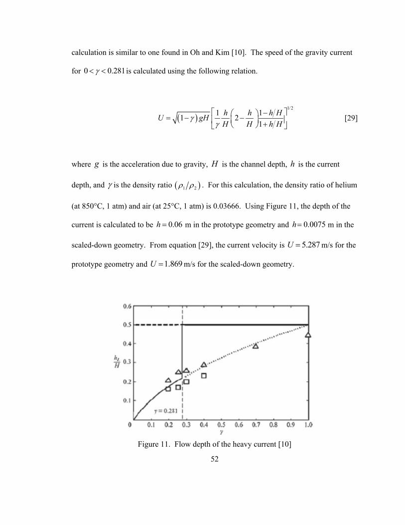
calculation is similar to one found in Oh and Kim [10]. The speed of the gravity current

for 0 0.281 is calculated using the following relation.

1/2

1 11 2

1

h h h HU gH

H H h H

[29]

where g is the acceleration due to gravity, H is the channel depth, h is the current

depth, and is the density ratio 1 2 . For this calculation, the density ratio of helium

(at 850°C, 1 atm) and air (at 25°C, 1 atm) is 0.03666. Using Figure 11, the depth of the

current is calculated to be 0.06h m in the prototype geometry and 0.0075h m in the

scaled-down geometry. From equation [29], the current velocity is 5.287U m/s for the

prototype geometry and 1.869U m/s for the scaled-down geometry.

Figure 11. Flow depth of the heavy current [10]

53

To determine the density-driven air ingress time scale, a length scale needs to be

determined. Since the exact breaking point can change depending on the event, a

minimum time scale can be determined by taking the shortest possible distance.

Therefore, the length scale was determined to be one-half of hot exit plenum total length.

This is equal to L=3.4 m for the prototype geometry and L=0.425 m for the scaled-down

geometry. Originally, the density-driven time scale was compared to the air diffusion

time scale which assumes that the air is uniformly spread throughout the whole duct cross

section [10]. In order to achieve a more equitable time scale comparison, a superficial air

velocity was computed for the density-driven air ingress phenomenon. The superficial

velocities will be calculated for both geometry types even though the current analysis

does not consider the molecular diffusion time scale. The superficial velocity is

estimated by

s

UhU

H [30]

This is calculated to be 0.211 m/s for the prototype geometry and 0.075 m/s for the

scaled-down geometry. Therefore, the minimum density-driven air ingress time scale,

DD , is calculated by

DDs

L

U [31]

54

This equals 16.08 s for the prototype geometry and 5.68 s for the scaled-down geometry.

Since the Biot number is much less than 0.1, the error associated with using the

lumped capacitance method is negligible. Therefore, the thermal time constant, which

describes how quickly the temperature of the support column approaches the temperature

of the surroundings, is given by

pthermal

s

Vc

hA

[32]

where h, ρ, V, cp and As are the convective heat transfer coefficient, support column

density, support column volume, support column specific heat and support column

surface area, respectively. The thermal time scale for a wide range of parameters is

shown in Figure 12 and Figure 13. These two figures correspond to the prototypic and

scaled-down geometries, respectively. Since the exact value of the thermal time constant

is not nearly as important as its order of magnitude, an average of the 11 cases (each

value corresponding to a different air-helium mole fraction at 25°C) is the thermal time

constant used for this analysis. The thermal time constants for these 11 cases correspond

to the minimum thermal time constants for a given species composition. Therefore, the

average thermal time constant calculated in this analysis is a minimum average thermal

time constant. For the prototype geometry, the minimum average thermal time constant

is 14,008 s. For the scaled-down geometry, the minimum average thermal time constant

is 3,299 s.

55

Figure 12. Thermal time constant v. far-field temperature for prototype geometry

Figure 13. Thermal time constant v. far-field temperature for scaled-down geometry

0

10000

20000

30000

40000

50000

60000

0 100 200 300 400 500

Average

 Therm

al Tim

e Constan

t (s)

Far‐field Temperature, T∞(°C)

Average Thermal Time Constant v. Far‐field Temperature (Prototype; Ttop = 850°C)

100% He

90% He/10% Air

80% He/20% Air

70% He/30% Air

60% He/ 40% Air

50% He/50% Air

40% He/60% Air

30% He/70% Air

20% He/80% Air

10% He/90% Air

100% Air

2000

3000

4000

5000

6000

7000

8000

9000

0 100 200 300 400 500

Average

 Therm

al Tim

e Constan

t (s)

Far‐field Temperature, T∞(°C)

Average Thermal Time Constant v. Far‐field Temperature (Scaled‐down; Ttop = 850°C)

100% He

90% He/10% Air

80% He/20% Air

70% He/30% Air

60% He/40% Air

50% He/50% Air

40% He/60% Air

30% He/70% Air

20% He/80% Air

10% He/90% Air

100% Air

56

With the minimum density-driven air ingress time scale, DD , and minimum

thermal time constant, thermal , known, the minimum total time scale, total , can be

calculated. The total time scale is expressed as

1 1 1

total DD thermal [33]

The minimum density-driven air ingress time scale is three orders of magnitude smaller

than the thermal time constant for both types of geometry. This means that the minimum

total time scale is dominated by the density-driven air ingress time scale. Table 7

summarizes the time scales considered.

Geometry Type Density-driven Time Scale (s) Thermal Time Constant (s) Total Time Scale (s) Prototype 16.08 14,008 16.06

Scaled-down 5.68 3,299 5.67 Table 7. Summary of air-ingress phenomenon time scales

Support Column One-dimensional Heat Diffusion Transient Analysis

The one-dimensional fin analysis provided an axial temperature distribution of a

support column rod for a given set of boundary conditions. Calculating an average

temperature of the rod, heat transfer characteristics of the rod can be calculated such as

the Biot number, the heat transfer coefficient, and the transient conduction time scale.

The calculated Biot numbers and transient conduction time scales suggest that a lumped

capacitance approximation of the support column is valid. In order to confirm this

57

approximation and to establish an operational heater power for the shell/heater system, a

transient one dimensional analysis was performed on MATLAB.

The code (See Appendix B) utilizes a finite-difference discretization and an

explicit time-marching method. The discretization is derived using a uniform mesh.

Constant thermo-physical properties are assumed for this calculation. Density is taken to

be 1770 kg/m3. Specific heat capacity is taken to be 1720 J/(kg·K). Thermal conductivity

is taken to be 85 W/(m·K). These thermo-physical properties correspond to a IG-110

graphite temperature of 750°C [32]. The governing equation is a single spatial dimension

(radial variable) transient heat diffusion equation for cylindrical coordinates.

Mathematically, this is expressed as follows:

1 2

1; ; 0p

T Tc kr r r r t

t r r r

[34]

where 1 2,r r is the inner and outer radius of the column/annulus, respectively. The radial

variable is normalized on Figure 14 - Figure 19 for easier comparison among the different

geometries. Table 8 lists the boundary and initial conditions for cases (1), (2) and (3).

Case Left Boundary

Condition Right Boundary Condition Initial Condition

1

0

0r

T

r

2

2( , )sr r

Tk h T r r t T

r

( , 0) 750 oT r t C

2

3 1

s heaterr r

Tk q

r

Table 8. Boundary conditions and initial condition for transient one-dimensional analysis

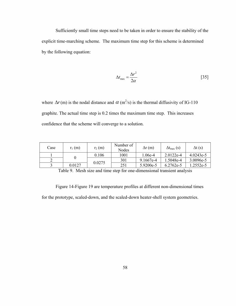
58

Sufficiently small time steps need to be taken in order to ensure the stability of the

explicit time-marching scheme. The maximum time step for this scheme is determined

by the following equation:

2

max 2

rt

[35]

where r (m) is the nodal distance and (m2/s) is the thermal diffusivity of IG-110

graphite. The actual time step is 0.2 times the maximum time step. This increases

confidence that the scheme will converge to a solution.

Case r1 (m) r2 (m) Number of

Nodes Δr (m) Δtmax (s) Δt (s)

1 0

0.106 1001 1.06e-4 2.0122e-4 4.0243e-5 2

0.0275 301 9.1667e-4 1.5048e-4 3.0096e-5

3 0.0127 251 5.9200e-5 6.2762e-5 1.2552e-5 Table 9. Mesh size and time step for one-dimensional transient analysis

Figure 14-Figure 19 are temperature profiles at different non-dimensional times

for the prototype, scaled-down, and the scaled-down heater-shell system geometries.

59

Figure 14. Radial temperature profile for prototype geometry at different times (t/τtotal)

Figure 15. Radial temperature profile for scaled-down geometry at different times (t/τtotal)

0 0.1 0.2 0.3 0.4 0.5 0.6 0.7 0.8 0.9 1743

744

745

746

747

748

749

750

751

Normalized Radial Distance from Support Column Centerline

Tem

pera

ture

(o C)

Temperature v. Normalized Radial Position (Prototype)

t/ = 0

t/=0.05

t/=0.10

t/=0.25

t/=0.50

t/=1.00

t/=1.50

t/=2.00

t/=2.50

t/=3.00

0 0.1 0.2 0.3 0.4 0.5 0.6 0.7 0.8 0.9 1743

744

745

746

747

748

749

750

751

Normalized Radial Distance from Support Column Centerline

Tem

pera

ture

(o C)

Temperature v. Normalized Radial Position (Scaled-down Geometry)

t/ = 0

t/=0.05

t/=0.10

t/=0.25

t/=0.50

t/=1.00

t/=1.50

t/=2.00

t/=2.50

t/=3.00

60

Figure 16. Radial temperature profile for shell/heater system at heater power of 150 W

Figure 17. Radial temperature profile for shell/heater system at heater power of 125 W

0 0.1 0.2 0.3 0.4 0.5 0.6 0.7 0.8 0.9 1743

744

745

746

747

748

749

750

751

Normalized Radial Distance from Support Column Centerline

Tem

pera

ture

(o C)

Temperature v. Normalized Radial Position (Shell/Heater System)

t/ = 0

t/=0.05

t/=0.10

t/=0.25

t/=0.50

t/=1.00

t/=1.50

t/=2.00

t/=2.50

t/=3.00

0 0.1 0.2 0.3 0.4 0.5 0.6 0.7 0.8 0.9 1743

744

745

746

747

748

749

750

751

Normalized Radial Distance from Support Column Centerline

Tem

pera

ture

(o C)

Temperature v. Normalized Radial Position (Shell/Heater System)

t/ = 0

t/=0.05

t/=0.10

t/=0.25

t/=0.50

t/=1.00

t/=1.50

t/=2.00

t/=2.50

t/=3.00

61

Figure 18. Radial temperature profile for shell/heater system at heater power of 100 W

Figure 19. Radial temperature profile for shell/heater system at heater power of 0 W

0 0.1 0.2 0.3 0.4 0.5 0.6 0.7 0.8 0.9 1743

744

745

746

747

748

749

750

751

Normalized Radial Distance from Support Column Centerline

Tem

pera

ture

(o C)

Temperature v. Normalized Radial Position (Shell/Heater System)

t/ = 0

t/=0.05

t/=0.10

t/=0.25

t/=0.50

t/=1.00

t/=1.50

t/=2.00

t/=2.50

t/=3.00

0 0.1 0.2 0.3 0.4 0.5 0.6 0.7 0.8 0.9 1743

744

745

746

747

748

749

750

751

Normalized Radial Distance from Support Column Centerline

Tem

pera

ture

(o C)

Temperature v. Normalized Radial Position (Shell/Heater System)

t/ = 0

t/=0.05

t/=0.10

t/=0.25

t/=0.50

t/=1.00

t/=1.50

t/=2.00

t/=2.50

t/=3.00

62

There is good agreement among Figure 14-Figure 19. The temperature profile

varies negligibly over the radius of the rod/annulus. Therefore, the lumped capacitance

method is a good approximation. Also, a heater power of 125 W creates a temperature

profile through the annular portion of the scaled-down rod-heater system (Figure 17)

similar to that shown in the scaled-down support column (Figure 15) and the prototypic

support column (Figure 14). It should be noted, however, that even if 0 W is pushed

through the heater there is a very good similarity between the temperature profiles of the

shell/heater system, scaled-down rod and prototype rod. Therefore, there exists a heater

power that can be utilized during the course of an experiment such that similar

temperature profiles can be achieved among the three different support column

geometries. This preserves the natural circulation phenomenology of the prototype during

the course of an experiment on the scaled-down facility.

Support Column Two-dimensional Heat Diffusion Transient Analysis

In addition to the one-dimensional transient analysis, a two-dimensional transient

analysis was performed. The major difference between the current analysis and the 1-D

transient analysis is that the current analysis takes into account a heat source. More

specifically, the current analysis takes into account the heat conducted at the top and the

bottom boundaries of the support column. Mathematically, this is demonstrated by

imposing fixed temperature (Dirichlet) boundary conditions at the top and bottom

boundaries of the support column. The governing equation is a two-dimensional heat

diffusion transient equation for cylindrical coordinates.

63

Mathematically,

1 2

1; ; 0p

T T Tc kr k r r r t

t r r r z z

[36]

For cases (1) - (3) as defined in the 1-D transient analysis, the boundary conditions are

summarized in Table 10.

Case Top

Boundary Condition

Bottom Boundary Condition

Left Boundary Condition

Right Boundary Condition

1

Fixed Temperature

(750°C)

Fixed Temperature

(750°C)

0

0r

T

r

2

2( , , )sr r

Tk h T r r z t T

r

2

3 1

s heaterr r

Tk q

r

Table 10. Boundary conditions for two-dimensional analysis

The same initial condition is imposed on the rod/annulus that is imposed in the 1-D

transient analysis. Namely,

1 2( , , 0) 750 ; ; 0oT r z t C r r r z H [37]

The total time scale, heat transfer coefficient and far-field temperature for the 2-D

analysis are given in Table 11. The total time scales are taken from Table 7. The heat

64

transfer coefficients are the largest values calculated from the 1-D fin analysis. The far-

field temperature is the lowest value considered in the 1-D fin analysis.

 

Table 11. Total time scale, convective heat transfer coefficient, and far-field temperature for case (1), (2), and (3)

Under these conditions, this allows for the maximum possible heat removal from a

support column. So, if a temperature profile is relatively flat under these conditions, it is

certain that the lumped capacitance approximation is valid under all other possible

conditions within the scope of the experiment. Furthermore, it determines the maximum

required heater power to maintain temperature profile similarity in the shell/heater

system.

The governing equation is discretized using a finite volume discretization and

explicit time-marching scheme. The stability is ensured by taking t to be 0.2 of maxt

where

max

2 2

11 1

2t

r z

[38]

Case Total Time Scale (s) Heat Transfer

Coefficient (W/(m2K)) Far-field Temperature

(°C) 1 16.06 12.688

25 2 5.67 15.571

3

65

is the largest thermal diffusivity of IG-110 graphite over the range of 20–800°C, r is

the horizontal mesh spacing and z is the vertical mesh spacing. This yields the smallest

maxt . The largest value occurs at 20°C and equals 1e-4 m2/s. The mesh size and

corresponding maxt are shown for each case in Table 12.

Case

Support Column

Inner Radius, r1 (m)

Support Column Outer

Radius, r2 (m)

Support Column Height, H (m)

Number of Cells

in Radial Direction

Number of Cells in Axial

Direction

Δr (m) Δz (m) Δtmax (s) Δt (s)

1 0

0.106 2.84 40 1000 0.0027 0.0028 0.0188 0.0038 2

0.0275 0.3556 40 200 6.88e-4 0.0018 0.0021 4.11e-4

3 0.0148 20 200 7.40e-4 0.0018 0.0023 4.67e-4 Table 12. Mesh size and time step for two-dimensional transient analysis

Using this method, temperature contour plots have been generated for cases (1)–

(3) at time 3 totalt . To simplify comparison, the radial and axial direction (or x- and y-

axis, respectively) have been normalized with respect to the case’s column geometry.

Also, the thermal conductivity and specific heat capacity are not constant, but vary with

temperature. Correlations were derived from data in the available literature [32].

Density is taken to be 1770 kg/m3. Both the thermal conductivity and specific heat

capacity for the IG-110 graphite are expressed in the following relations:

8 3 5 23 10 1 10 0.0612 125.56sk T T T T [39]

7 3 2( ) 9 10 0.0027 3.0203 643.24pc T T T T [40]

66

where T is in units of °C. Equations [39] and [40] are valid for the temperature range of

20–800°C. Figure 20 - Figure 25 are the resulting temperature contour plots of the 2-D

analysis at 3 totalt . Figure 20 is the temperature contour plot for the prototype

geometry. Figure 21 is the temperature contour plot for the scaled-down geometry.

Figure 22-Figure 25 are temperature contour plots for the shell/heater system at Q = 150

W, 125 W, 100 W, and 0 W, respectively.

Figure 20. Temperature contour plot for prototype geometry (Case 1) at t=3τtotal

Normalized Radial Distance from Support Column Centerline

Nor

mal

ized

Axi

al D

ista

nce

from

Sup

port

Col

umn

Bot

tom

Temperature (oC) v. Position (Prototype; t = 3)

0.1 0.2 0.3 0.4 0.5 0.6 0.7 0.8 0.9

0.1

0.2

0.3

0.4

0.5

0.6

0.7

0.8

0.9

745

745.5

746

746.5

747

747.5

748

748.5

749

749.5

67

Figure 21. Temperature contour plot for scaled-down geometry (Case 2) at t = 3τtotal

Figure 22. Temperature contour plot for shell/heater system for 150 W (Case 3a) at

t=3τtotal

Normalized Radial Distance from Support Column Centerline

Nor

mal

ized

Axi

al D

ista

nce

from

Sup

port

Col

umn

Bot

tom

Temperature (oC) v. Position (Scaled-down Geometry; t = 3)

0.1 0.2 0.3 0.4 0.5 0.6 0.7 0.8 0.9

0.1

0.2

0.3

0.4

0.5

0.6

0.7

0.8

0.9

745

745.5

746

746.5

747

747.5

748

748.5

749

Normalized Radial Distance from Support Column Centerline

Nor

mal

ized

Axi

al D

ista

nce

from

Sup

port

Col

umn

Bot

tom

Temperature (oC) v. Position (Shell/Heater System; t = 3; Qdot = 150 W)

0 0.1 0.2 0.3 0.4 0.5 0.6 0.7 0.8 0.9

0.1

0.2

0.3

0.4

0.5

0.6

0.7

0.8

0.9

745

745.5

746

746.5

747

747.5

748

748.5

749

68

Figure 23. Temperature contour plot for shell/heater system for 125 W (Case 3b) at

t=3τtotal

Figure 24. Temperature contour plot for shell/heater system for 100 W (Case 3c) at

t=3τtotal

Normalized Radial Distance from Support Column Centerline

Nor

mal

ized

Axi

al D

ista

nce

from

Sup

port

Col

umn

Bot

tom

Temperature (oC) v. Position (Shell/Heater System; t = 3; Qdot = 125 W)

0 0.1 0.2 0.3 0.4 0.5 0.6 0.7 0.8 0.9

0.1

0.2

0.3

0.4

0.5

0.6

0.7

0.8

0.9

745

745.5

746

746.5

747

747.5

748

748.5

749

Normalized Radial Distance from Support Column Centerline

Nor

mal

ized

Axi

al D

ista

nce

from

Sup

port

Col

umn

Bot

tom

Temperature (oC) v. Position (Shell/Heater System; t = 3; Qdot = 100 W)

0 0.1 0.2 0.3 0.4 0.5 0.6 0.7 0.8 0.9

0.1

0.2

0.3

0.4

0.5

0.6

0.7

0.8

0.9

745

745.5

746

746.5

747

747.5

748

748.5

749

69

Figure 25. Temperature contour plot for shell/heater system for 0 W (Case 3d) at t=3τtotal

The results of the 2-D calculations are promising and, in many respects, give

similar conclusions to those found in the 1-D transient analysis. At first glance, the

average temperature gradient in the radial direction at the mid-plane for all six cases is

similar. Table 13 quantifies the average radial temperature gradient for Figure 20 -

Figure 25. Please note that the non-dimensional radial thickness is defined as 2 1

2

r r

r

.

Table 13. Temperature gradient at the vertical mid-plane of the support column

Normalized Radial Distance from Support Column Centerline

Nor

mal

ized

Axi

al D

ista

nce

from

Sup

port

Col

umn

Bot

tom

Temperature (oC) v. Position (Shell/Heater System; t = 3; Qdot = 0 W)

0 0.1 0.2 0.3 0.4 0.5 0.6 0.7 0.8 0.9

0.1

0.2

0.3

0.4

0.5

0.6

0.7

0.8

0.9

744

744.5

745

745.5

746

746.5

747

747.5

748

748.5

749

Case Heater

Power (W) Non-dimensional Radial Thickness

Radial Thickness (m)

Temperature Difference

oC

oT C

r m

1 N/A 1

0.106 3.5 33.02 2 N/A 0.0275 0.75 27.28 3a 150

0.5382 0.01480

0.75 50.68 3b 125 0.75 50.68 3c 100 0.625 42.23 3d 0 0.5 33.78

70

From Table 13, Case 3d is the best case for simulating the average radial thermal gradient

at the midplane. This suggests that case 3d, whose heater power is 0 W, has the closest

average radial heat flux to that of the scaled-down and prototypic support columns.

The surface temperature for a majority of the support column for all six cases is

within one degree celsius. Outside this region, the surface temperature does not increase

more than five degrees celsius for any of the geometries. Case 3b ( Q = 125 W),

however, appears to have the most similar surface temperature distribution to those found

in the prototypical and scaled-down geometries. It’s interesting to note that even if no

power is pushed through the heater in the shell/heater system, there’s still good similarity

of the surface temperature distribution at t = 3τtotal among all three geometry types.

Beyond t = 3τtotal, the change in the temperature contour plots would be more distinct

among the three different geometries given the mass difference of each geometry type. If

it’s necessary to run the experiments past this time limit (t = 3τtotal ), additional

calculations would need to be performed to see the maximum required heater power to

simulate the temperature profiles in the prototypic and scaled-down geometries.

However, up to t = 3τtotal , the surface temperature distribution of the shell/heater system

is most similar to the surface temperature distribution of the prototype and scaled-down

support columns when the heater is emitting 125 W (Case 3b).

In conclusion, if the heater power is 0 W (Case 3d), this creates the closest

average radial heat flux at the mid-plane of the shell/heater system to those average radial

heat fluxes found at the mid-plane of the prototypic and scaled-down support columns

(Case 1 & Case 2), as seen in Table 13. On the other hand, if the heater were emitting

71

125 W of power, a surface temperature distribution along the shell/heater system would

be created that is the most similar to the surface temperature distribution of the prototypic

and scaled-down support columns.

Design Analysis of Containment

Following a depressurization of the pressure vessel, hot helium from the reactor

vessel mixes in the vessel’s containment with relatively cool air from the reactor cavity.

The mixing process creates a mixed species temperature as well as a mixed species

concentration which have a significant effect on the following stages of an air-ingress

accident especially the density-driven stratified flow. In this analysis, considerations are

made to calculate the free volume of the scaled-down containment and the initial pressure

of the scaled-down vessel. By calculating the values, the final mixing temperature and

air-to-helium mole ratio in the prototypic case will be preserved in the scaled-down case.

Furthermore, with an understanding of the initial pressure of the scaled-down vessel, the

initial operating conditions for a given experiment are now determined.

Utilizing the prototypic geometry and normal operating conditions of the GT-

MHR, it was found that the mole ratio of air in the containment to helium in the pressure

vessel is 5.15. In order to maintain this mole ratio, the containment volume of the scaled-

down geometry was calculated for different initial vessel pressures. In these calculations,

the volume of the prototypic containment is taken to be 25,000 m3, the free volume of the

pressure vessel is taken to be 265 m3. The initial pressure and temperature of the vessel

is 7 MPa and 850°C, respectively. The initial pressure and temperature of the

containment is 0.101325 MPa and 25°C, respectively. The free volume of the scaled-

72

down vessel is 0.210 m3. The initial helium temperature is 750°C in the scaled-down

pressure vessel. In these calculations, the temperature and pressure of the scaled-down

containment are the same as those for the prototype containment. The ideal gas law was

used to calculate the free volume of the scaled-down containment so that the air to helium

mole ratio is the same that is found in the prototypic case. The results are summarized in

Table 14 for different initial vessel pressures.

Initial Scaled-down Vessel Pressure (psig)

Initial Vessel Temperature (°C)

Scaled-down Containment Volume (m3)

0 750 0.315 30 750 0.963 60 750 1.605

Table 14. Scaled-down containment free volume for different initial vessel pressures

In addition to the above analysis, the mixed mean temperature of the pressure

vessel containment system is calculated by using the first law of thermodynamics,. This

analysis was performed to give the final temperature of the air-helium mixture after the

helium is emptied into the containment. This temperature occurs after the contents are

well mixed. It’s also assumed that that no heat is lost or gained from the confinement and

that no work is done by the control volume which makes sense since it’s a rigid volume.

The governing equation is given by

0f iU U [41]

73

where fU , iU are the internal energy of the system at the final and initial stages,

respectively. By manipulating equation [41], the final temperature of the system can be

solved as seen in equation [42].

, , , ,

, ,

i i

f f

he v he i he a v a i a

f

he v he a v a

m c T m c TT

m c m c

[42]

Since the specific heat of air is a function of temperature, equation [42] is solved

iteratively. Using the initial conditions listed in Table 15, the final temperature is 382.6

K. Using the ideal gas law, the final pressure is 0.1538 MPa.

Confinement Pressure Vessel Pressure (MPa) 0.101325 7 Volume (m3) 25,000 265 Temperature (K) 300 1123 Species 100% Air 100% Helium

Table 15. Initial conditions for final temperature analysis

In the GT-MHR containment, there are vents located on the wall. Therefore, the

global pressure within the containment is maintained at or very near atmospheric

pressure. Since the final pressure in the first law analysis is above atmospheric pressure,

a transient control volume analysis was performed. The governing equation is given in

equation [43]. It is assumed that only air escapes out of the containment and it does so at

its initial temperature.

74

f i e eU U m h [43]

Rearranging equation [43], the final temperature can be solved for as seen in equation

[44].

, , , , , , ,

, , ,

i i i

f f

e p a i a he v he i he a i v a i a

f

he v he a f v a

m c T m c T m c TT

m c m c

[44]

where , ,e a i a fm m m . Iterating over equation [44] and using the ideal gas law, a final

temperature can be found. All final pressures are atmospheric pressure. A summary of

the results can be found in Table 16. Different cases are based on the initial vessel

pressure in the scaled-down facility.

Geometry Type (Initial Vessel Pressure)

Final Temperature (K) Percent of Initial Air Mass Lost

Final Air/He Mole Ratio

Prototype (7 MPa) 366 37.2% 3.22 Scaled-down (60 psig) 406.2 42.4% 1.85 Scaled-down (53.4 psig) 394.7 37.1% 2.21 Scaled-down (40 psig) 374.0 26.5% 3.21 Scaled-down (34.2 psig) 366.0 21.9% 3.81 Scaled-down (30 psig) 360.5 18.7% 4.34 Scaled-down (0 psig) 327.1 -4.0% 16.67

Table 16. Results of transient control volume analysis following depressurization

From Table 16, it can be seen that the final temperature of the prototype geometry

can be attained when the initial vessel pressure of the scaled-down vessel is 34.2 psig and

75

a containment free volume of 1 m3. The final air-to-helium mole ratio of the prototype

geometry can be attained in the scaled-down geometry when the initial vessel pressure is

40 psig. The air-to-helium mole ratio is also an important aspect of this analysis since the

density, viscosity, thermal conductivity and specific heat of the air/helium mixture are

dependent on the mole fractions of these two species. Less importantly, the percentage of

air mass lost from the containment can be simulated if the initial vessel pressure in the

scaled-down system is 53.4 psig.

Transient Blowdown Analysis

In the event of a LOCA of a GT-MHR, the pressure boundary of the reactor is

compromised. Under such circumstances, the reactor initially undergoes a

depressurization or blowdown in which helium in the reactor system empties into the

surroundings, namely, a containment that houses the reactor vessel. In this analysis,

helium is released from the reactor vessel through a break in the cross vessel of the

reactor. It will be shown that the blowdown is a rapid process whose time scale is much

shorter than the time scale of the density-driven stratified flow and hot plenum natural

circulation.

During the release of helium, the temperature of the fluid initially decreases with

time due to the expansion of the helium inside the vessel. As the pressure of the helium

inside the vessel approaches the ambient pressure, the heat transferred from the reactor

internals and vessel wall to the fluid cause the temperature of the fluid to increase. The

interaction of these two effects leads to a dynamic behavior of the fluid temperature

during the depressurization process.

76

In the present analysis, a simple model for describing the depressurization process

of a helium-filled reactor vessel with internal structures has been employed. This simple

method does not incorporate local details such as flow patterns or temperature fields, but,

instead, uses a lumped capacitance model to reveal the integral changes taking place

during the depressurization. Also, this simplified model assumes constant thermo-

physical properties except for density and a constant heat transfer coefficient between the

solid structures and the helium. Since natural convection is the dominant mode of heat

transfer during a depressurization, the heat transfer coefficient is taken to be 2 W/(m2·K).

The energy conservation equations for helium and the internal solid structures are given

in equation [45] and [46], respectively.

( ( ) ( ))( )( ) ( ) ( ( ) ( )) ( ) ( )v

conv s w p

d m t c T tdU tQ t mi t hA T t T t m t c T t

dt dt [45]

where i is the helium enthalpy, and h is the heat transfer coefficient [33]. For all solid

structures (vessel wall and internals), the energy equation is

0.2, 0

( )( ) ( ) 0.066 ( ( ) ( ))w w

gen conv w w p w s w

dH t dTQ t Q t V c P t hA T t T t

dt dt [46]

where oP is the constant operating power level, and wT is the wall temperature. The

mass balance equation is simply

77

( ) ( )o o exitm t m m t dt m m t [47]

The density as a function of time is derived by dividing equation [47] by the free volume

of the vessel. It is shown in equation [48].

1( ) ( ) exit

o o

mt m t dt t

V V

[48]

By taking t to be sufficiently small, ( )m t can approximated as a constant. This way,

the use of integrals can be avoided in the MATLAB code (See Appendix B). From the

momentum equation for steady incompressible flow,

2 21 1 2 2

1 1 2 22 2 L

p V p Vz z h

g g

[49]

the velocity as it leaves the hot duct can be derived where Lh is the head loss for the flow

from the vessel to the containment. It takes into account the sudden contraction from the

vessel to the hot duct and the friction along the duct. The velocity out of the hot duct can

be expressed as

( )( )

1

2 2

amb

avg ch

P t Pv t

f lK

D

[50]

78

where is the kinetic energy coefficient and cK is the pressure loss coefficient for a

sudden contraction. The kinetic energy coefficient is taken to be one which corresponds

to a flat velocity profile. This is a fair approximation since the flow through the duct is

turbulent.

The state equation is the ideal gas law shown in equation in [51].

( ) ( ) ( )P t t R T t [51]

The initial conditions are as follows:

, , , 0i i i w im m P P T T T T at t [52]

Equations [45]–[48], [50] and [51] can be rewritten in their discretized form as

shown in equations [53]-[58].

Helium Temperature

( )( 1) ( ) 1 ( )

( ) ( )ss

wv v

hA m i R thA tT i T i T i

c m i c m i

[53]

79

Temperature of Vessel Wall and Internals

2 0.20

, , ,

0.066 (( 1) )( 1) ( ) 1 ( )s s

w ww w p w w w p w w w p w

t P i t t hA t hA tT i T i T i

V c V c V c

[54]

Helium Mass in Vessel

( 1) ( ) ( )m i m i m i t [55]

Helium Density in Vessel

( )( 1) ( )

m ii i t

V

[56]

Helium Exit Velocity

( )( )

1

2 2

amb

avg ch

P i Pv i

f lK

D

[57]

Helium Pressure

( 1) ( 1) ( 1)p i i R T i [58]

From initial conditions in equation [52], the velocity as seen in equation [57] can

be calculated. If the velocity is greater than or equal to the speed of sound than the mass

flow is calculated based on the choked flow velocity; otherwise, the mass flow rate is

based the calculated velocity. With the mass flow rate and other given or calculated

80

parameters, the helium temperature and “wall” temperature can be calculated from

equations [53] and [54]. Furthermore, the helium mass and density in the vessel can be

calculated based on equations [55] and [56], respectively. Finally, a new helium pressure

is calculated based on the new helium density and temperature. The process is repeated

until the helium pressure is equal to the ambient pressure.

Figure 26 through Figure 28 show the helium pressure in the vessel, the helium

temperature in the vessel and temperature of the vessel wall and internal structures as a

function of time during a blowdown event following a double-ended guillotine break.

There are three distinct curves on each figure corresponding to different heat transfer

coefficients. This is for the prototypic geometry and conditions. Initial temperature of

the helium and the vessel internal structures is 850°C (1123.15 K) and the initial vessel

pressure is 7 MPa.

81

Figure 26. Pressure versus time during depressurization of prototypic vessel

Figure 27. Helium temperature versus time during depressurization of prototypic vessel

0 0.05 0.1 0.15 0.2 0.25 0.3 0.35 0.4 0.45 0.50

1

2

3

4

5

6

7x 10

6

Time (s)

Pre

ssur

e (P

a)

Prototype Geometry - Pressure v. Time

h = 2 W/(m2*K)

h = 10 W/(m2*K)

h = 40 W/(m2*K)

0 0.5 1 1.5 2 2.5 3 3.5 4 4.5 5200

300

400

500

600

700

800

900

1000

1100

1200

Time (s)

Hel

ium

Tem

pera

ture

(K

)

Prototype Geometry - Helium Temperature v. Time

h = 2 W/(m2*K)

h = 10 W/(m2*K)

h = 40 W/(m2*K)

82

Figure 28. “Wall” temperature versus time during depressurization of prototypic vessel

From Figure 26, it can be observed that the blowdown is essentially over in 0.3 s

for all three heat transfer coefficients. The duration of the blowdown is two orders of

magnitude smaller than the density-driven air ingress time scale and five orders of

magnitude smaller than the hot plenum natural circulation time scale. This means that

the duration of the blowdown is two orders of magnitude smaller than the total time scale,

total . Therefore, the duration of the blowdown is negligible when compared to the total

time scale of the air-ingress accident (See Table 7) in the prototype geometry. However,

as seen in Figure 27, there’s a significant decrease in the helium temperature during the

blowdown process due to the net loss in thermal energy from the helium due to its

expansion. It can also be seen that temperature of the helium in the vessel is dependent

on the heat transfer coefficient. With higher heat transfer coefficients, more thermal

0 0.5 1 1.5 2 2.5 3 3.5 4 4.5 5

1123.12

1123.13

1123.14

1123.15

1123.16

1123.17

1123.18

Time (s)

Sol

id T

empe

ratu

re (

K)

Prototype Geometry - Solid Temperature v. Time

h = 2 W/(m2*K)

h = 10 W/(m2*K)

h = 40 W/(m2*K)

83

energy is released from the vessel internal structures into the helium. This causes the

local minimum of the helium temperature to increase as the heat transfer coefficients

increases. Also, the time derivative of the helium temperature increases as the heat

transfer coefficient increases. This means that with a higher heat transfer coefficient the

density difference between helium within the vessel and the air-helium mixture in the

containment will be greater, causing the plume in the density-driven stratified flow to

ingress more quickly. Figure 28 shows that the change in temperature of the vessel’s

internal structures is minimal over the duration of the blowdown despite the heat transfer

coefficient. These results indicate the importance of knowing the helium temperature at

the end of the blowdown phase and the temperature of the air-helium mixture at the end

of the blowdown. It is these two temperatures and their corresponding densities that will

determine how quickly the density-driven stratified flow will occur.

Figure 29 through Figure 31 show the helium pressure in the vessel, the helium

temperature in the vessel and temperature of the vessel wall and internal structures as a

function of time during a blowdown event following a double-ended guillotine break.

There are three distinct curves on each figure corresponding to different heat transfer

coefficients. This is for the scaled-down geometry and conditions. Initial temperature of

the helium and the vessel internal structures is 750°C (1023.15 K) and the initial vessel

pressure is 75 psia or 517106 Pa.

84

Figure 29. Pressure versus time during depressurization of scaled-down test section

Figure 30. Helium temperature versus time during depressurization of scaled-down test

section

0 0.001 0.002 0.003 0.004 0.005 0.006 0.007 0.008 0.009 0.010

0.5

1

1.5

2

2.5

3

3.5

4

4.5

5

5.5x 10

5

Time (s)

Pre

ssur

e (P

a)

Scaled-down Test Section - Pressure v. Time

h = 2 W/(m2*K)

h = 10 W/(m2*K)

h = 40 W/(m2*K)

0 0.05 0.1 0.15500

600

700

800

900

1000

1100

Time (s)

Hel

ium

Tem

pera

ture

(K

)

Scaled-down Test Section - Helium Temperature v. Time

h = 2 W/(m2*K)

h = 10 W/(m2*K)

h = 40 W/(m2*K)

85

Figure 31. “Wall” temperature versus time during depressurization of scaled-down test

section

Figure 29 shows that the blowdown in the scaled-down test facility terminates in

approximately 0.008 s for all three heat transfer coefficients. The duration of the

blowdown is three orders of magnitude smaller than the density-driven stratified flow and

six orders of magnitude smaller than the hot plenum natural circulation in the scaled-

down geometry. This means that the duration of the blowdown is three orders of

magnitude smaller than the total time scale, total . Therefore, the duration of the

blowdown is negligible when compared to the total time scale of the air-ingress accident

in the scaled-down test section (See Table 7). Comparing Figure 27 and Figure 30, it can

be seen that there’s a significant difference between the helium temperature in the

prototype and the scaled-down geometry. This issue has been resolved by preserving the

0 0.05 0.1 0.151023.1482

1023.1484

1023.1486

1023.1488

1023.149

1023.1492

1023.1494

1023.1496

1023.1498

1023.15

1023.1502

Time (s)

Sol

id T

empe

ratu

re (

K)

Scaled-down Test Section - Solid Temperature v. Time

h = 2 W/(m2*K)

h = 10 W/(m2*K)

h = 40 W/(m2*K)

86

non-dimensional Froude number over that temperature range. This is discussed in more

detail in the section Hydraulic Similarity in the Hot Duct-Hot Plenum System of Chapter

2. From Figure 31, the “wall” temperature varies negligibly during the duration of the

transient for all three heat transfer coefficients.

87

Chapter 3: Physical Description of the Scaled-down Facility

Introduction

With the critical dimensions of the scaled-down facility established, a design of

the experimental facility can be presented. The facility is essentially a one-eighth

geometric scaled-down model of the hot-exit plenum of the GT-MHR 600 MWth

constructed by General Atomics, Inc. Figure 32 shows clearly which region of the

reactor is modeled in the scaled-down facility.

Figure 32. Hot-exit plenum of the GT-MHR 600 MWth by General Atomics, Inc.

Scaled Model

88

All dimensions of the scaled-down facility are a one-eighth geometric scale

except for the hot duct length, the support column diameter, and the support column

pitch. The support column pitch and diameter are approximately one-fourth of the

prototype dimensions. The method for determining this factor was explained in Chapter

2. The hot duct length is 0.10 m or about 28% of the one-eighth scale which is 0.35 m.

This is done to maintain similarity of the loop pressure loss distribution between the

prototype and the scaled-down geometry.

Component Dimension (cm) Hot Duct Length 10.00

Hot Duct Inner Diameter 18.75 Support Column Diameter 5.5

Support Column Pitch 9.4 Test Section Inner Diameter 85.00

Test Section Height 35.50 Table 17. Critical dimensions for the scaled-down test facility

Design Drawings

Computer drawings are annotated to show the dimensions of each part of the

vessel. All parts to the vessel that are shown in Figure 33-Figure 48 are constructed of

Alloy 800H. Figure 33 is a side view of the bottom semi-hemispherical (2:1 elliptical

head) shell of the air-ingress experimental facility. The shell has an outside diameter of

34” and a height of 8.5”. The shell thickness is ¼”. Seventeen - ¾”, schedule 40 pipes

are welded to the bottom of the shell. These pipes are fabricated from Alloy 800H and

vary in length – the shortest being 8.5” long. All pipes, however, extend to the same

vertical level which is 17” below the top of the bottom semi-hemispherical shell. This

89

allows clearance for insulation to be placed along the bottom of the vessel without

interfering with the entrance of the instrumentation ports. Also, the additional distance

away from the vessel reduces the temperature requirements for the sealant of the Conax®

glands which will attach the thermocouples, pressure transducer tubing, and oxygen

sensors to the vessel while maintaining the pressure boundary of the entire system. The

reduced temperature requirement is also beneficial for the instrumentation by reducing

the possibility of an electrical failure.

Figure 33. Side view of the bottom semi-hemispherical shell

90

To determine an appropriate length of pipe, a 1-D fin calculation was performed

on the shortest pipe protruding from the bottom head 8.5”. This calculation shows that

with a base temperature of 750°C and a heat transfer coefficient of 2 W/(m2·K), the

temperature at the end of the pipe is about 650°C. The same calculation shows that with

a heat transfer coefficient of 5 W/(m2·K), the pipe-end temperature drops to 535°C.

These calculations suppose that one-half of the pipe length is wrapped in perfect

insulation. Although these temperatures are high and, in some situations, are too high for

the sealant of a Conax® gland (See Figure 34), this analysis does not take thermal

radiation into account. A Fluent calculation shows that when radiation is accounted for,

this greatly reduces the pipe-end temperature to 280°C. This corresponds to an effective

heat transfer coefficient 25 W/(m2·K). It is preferred to keep the facility as short as

possible for convenience in performing experiments, conducting maintenance, and

generally working around the facility. In the current design, if a three-foot clearance –

the distance from the bottom of the pipes to the floor - is taken into consideration, then

the overall height of the facility is 85 in. (2.159 m). A minimum three-foot clearance is

necessary in order to insert and extract instrumentation and instrumentation piping that

will need to be able to span a maximum distance of 31 in. (0.787 m). This is the distance

from the bottom of the pipe to the bottom of the top plate. The bottom semi-

hemispherical is welded to the bottom of the middle shell or test section shown in Figure

39 and Figure 40.

Figure 34 is a schematic of the Conax® gland used in the facility for sealing

pressure transducer tubing, oxygen sensors and thermocouples into the vessel. The

91

pressure transducer gland will seal two pressure transducer tubes per gland while the

thermocouple gland will seal four thermocouples per gland. An oxygen sensor gland will

seal a single oxygen sensor The metal housing is constructed of 303SST. The gland

sealant is made of Grafoil which operates up to 495°C in oxidizing environments.

Grafoil is a sealant which is made out of 99% pure graphite. 303SST has an annealing

temperature of 1010°C; this is well above the 280°C calculated pipe-end temperature.

Figure 34. Conax® gland at the end of the pipe on the bottom semi-hemispherical shell34

(Units: in.)

Figure 35 and Figure 36 are bottom views of the bottom semi-hemispherical shell

of the air-ingress experimental facility. Figure 36 shows the relative position of the

support columns to the instrumentation ports. The perforated lines represent the support

column position. Furthermore, in these figures, the type, position and spacing of the

instrumentation ports are shown.

92

Figure 35. Bottom view of the bottom semi-hemispherical shell

Figure 36. Bottom view of the bottom semi-hemispherical shell with support column

positions projected

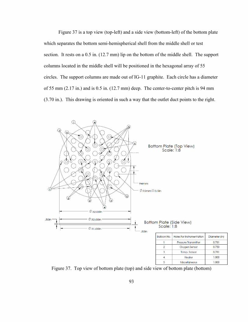
93

Figure 37 is a top view (top-left) and a side view (bottom-left) of the bottom plate

which separates the bottom semi-hemispherical shell from the middle shell or test

section. It rests on a 0.5 in. (12.7 mm) lip on the bottom of the middle shell. The support

columns located in the middle shell will be positioned in the hexagonal array of 55

circles. The support columns are made out of IG-11 graphite. Each circle has a diameter

of 55 mm (2.17 in.) and is 0.5 in. (12.7 mm) deep. The center-to-center pitch is 94 mm

(3.70 in.). This drawing is oriented in such a way that the outlet duct points to the right.

Figure 37. Top view of bottom plate (top) and side view of bottom plate (bottom)

94

Figure 38 is the bottom view of the bottom plate with and without the support

column positions projected onto the plate. The holes for the various types of

instrumentation are shown. The “heater” holes are in place to allow the unheated length

of the heater to protrude into the bottom semi-hemispherical shell. This permits the

heated length of the heater to coincide with the length of the support column. The

“miscellaneous” holes are in place to allow one to fill the bottom semi-hemispherical

shell with ¼” ceramic balls to take up the free volume in the lower shell. A chamfer is

used for each hole and its dimensions are outlined accordingly. The reason for the

chamfer is to facilitate the successful installation of the instrumentation into the test

section as it’s drawn up from the bottom. Note that the bottom plate is smaller in

diameter than the top plate so that both fit.

Figure 38. Bottom view of the bottom plate with (left) and without (right) support column positions projected

95

Figure 39 and Figure 40 show the middle shell or test section of the air-ingress

experimental facility. On the bottom of the shell, a lip is located that will support the

bottom plate (Figure 37 & Figure 38). A flange is welded around the top of the shell.

The top semi-hemispherical shell will be bolted to this flange. The duct with a flanged

end is located at the front. Extensions can be connected to the duct to simulate different

break types. An air piston will be used to secure the duct cover and initiate the accident

sequence. There are two 2-inch pipe extensions of approximately 7 in. in length on the

opposite side of the duct that are capped off with low pressure sight glasses whose

windows are constructed of quartz and whose metal fittings are constructed of 303SST

(See Figure 41). The pipe extensions are in place to allow insulation to be placed around

the vessel without interfering with the laser’s line of sight. The windows allow the laser

of the PIV/PLIF system to pass through to the test section while being able to maintain a

pressure boundary up to 1000 psi. This is more than sufficient for the experimental needs

of this project since the vessel will only be pressurized up to 50 psig. There’s also a ¾”

NPT pipe protruding from the bottom of the hot duct. This is an instrumentation port

where up to four thermocouples can be inserted into the hot duct.

96

Figure 39. Different views of the middle shell or test section

Figure 40. Bottom view (left) and side view (right) of middle shell

97

Figure 41. Low pressure sight glass on the side of the middle shell (B = 2.500 in., C =

1.875 in., D = 0.760 in., E = 0.290 in.) [35]

Figure 42. Top view of the top plate with (left) and without (right) support column

positions projected

98

Figure 42 is the top view of the top plate with (left) and without (right) the

support column positions projected. The top plate separates the middle shell from the top

semi-hemispherical shell which is shown in Figure 44 through Figure 46. The top side of

the plate has chamfers on the holes that are designed to allow the oxygen sensors and

heaters to pass through more easily to the test section. The two larger holes are for the

camera to take images with the PIV/PLIF system. Here, velocity and concentration

measurements are taken. The orientation of this drawing is such that the outlet duct is

pointed to the right.

Figure 43 shows a bottom view and a side view of the top plate. The hexagonal

array of holes is designed to secure the support columns. Each hole has a chamfer to

make it easier to secure the support column within the hole. This alignment is critical to

preserve the flow phenomenology. The 1” holes, in each support column anchor, are in

place to ensure that the support columns are correctly inserted to their proper position.

Figure 43. Bottom view (top) and side view (bottom) of the top plate

99

Figure 44 is a side view of the top semi-hemispherical shell. This piece is bolted

down to the middle shell as seen in Figure 39and Figure 40. There are 11 openings on

the top of the head –1 for insertion of ceramic balls, 2 for camera ports, 2 for oxygen

sensors, and 6 for heaters. All pipes extending from the shell end at the same vertical

level (17 inches above the shell bottom). This allows clearance for insulation to be

installed and relaxes the temperature requirement for the Conax® glands. It also reduces

the possibility of electrical failure in the instrumentation heads. A low pressure sight

glass as discussed for the laser ports (Figure 41) is used in the camera ports to maintain

the pressure boundary and still allow images to be taken by the camera. To fill the free

volume of the upper head, ceramic balls will be inserted from the top of the semi-

hemispherical shell. The ceramic balls (which are primarily aluminum oxide and silicon

dioxide) add a load of approximately 270 kg to the top plate. Even at the high

operational temperatures of 750°C, the added weight on the top plate produces a minimal

deflection of 0.0025”.

100

Figure 44. Side view of the top semi-hemispherical shell

Figure 45 and Figure 46 are a top view of the top semi-hemispherical shell without and

with the support column positions projected, respectively. These figures show the type,

position and relative spacing of the ports with respect to each other and, in the case of

Figure 46, the support columns. For both figures, they are oriented such that the outlet

duct is pointing right.

101

Figure 45. Top view of the top semi-hemispherical shell

Figure 46. Top view of top semi-hemispherical shell with support column positions

projected

102

Figure 47 and Figure 48 show a side view and a side cut view of the assembled vessel,

respectively.

Figure 47. Side view of the assembled vessel

Figure 48. Side cut view of the assembled vessel

103

Instrumentation of the Physical Setup

Instrumentation is essential to any experiment. In the following paragraphs, the

different types of instrumentation will be discussed. The location of the instrumentation

within the scaled-down test facility has been shown in Figure 33 through Figure 48.

There are four major parameters that will be measured in the facility – pressure,

temperature, oxygen concentration and local gas velocity.

Pressure

The most straight-forward instrumentation for the facility are the pressure and

temperature sensors. To measure pressure in the vessel, Honeywell STG944 Pressure

(Gage) Transducers are used. The transducers are used to measure pressure inside the

middle shell (or test section) as seen in Figure 39 and Figure 40. During density-driven

air ingress and hot plenum natural circulation, large pressure variations from atmospheric

pressure are not expected occur. However, that instrumentation will be in place to

measure the gage pressure at different locations throughout the vessel which consists

mainly of the lower plenum of the reactor vessel. The pressure tubing can be moved

vertically if measurements need to be made at different vertical positions. The transducer

is also used to measure the pressure dynamics during the initial depressurization phase of

the experiments.

Table 18. Pressure transducer specifications

Pressure Range Temperature Range Output Range Frequency Response 0 – 500 psi -40 - 110°C 4 - 20 mA 350 ms (Analog mode)

104

In analog mode, the accuracy of the pressure transducer is ±0.075% of the calibrated span

or upper range value, whichever is greater. In digital mode, the accuracy of the pressure

transducer is ±0.0625% of the calibrated span or upper range value, whichever is greater.

Figure 49. Schematic of Honeywell STG944 Pressure Transducer [36]

Temperature

For temperature measurements, a grounded Type N thermocouple constructed by

OMEGA is used. The thermocouples have a quick response time (0.55 s) and can handle

temperatures up to 1335°C. The accuracy of the thermocouple is ±1.1°C or ±0.40% of

105

the reading, whichever is greater. Their location is shown clearly on Figure 33 and

Figure 36. A row of thermocouples is placed along the midline extended from the hot

duct to capture the plume as it moves across the bottom of the test section. Another row

of thermocouples is perpendicular to the previous row. This arrangement is to capture

temperature information with respect to the plume’s width as the front moves across the

bottom of the lower plenum. As in the case of the pressure tubing, the thermocouples can

be moved vertically if measurements need to be made at different vertical positions.

Oxygen Sensors

Oxygen concentration instrumentation suitable for the current application is a

challenging technical issue. An extensive search was performed to find the best

candidates for the experimental facility. In-situ oxygen sensors seemed to be the best

type of oxygen sensor since they generally had the lowest response times. However, the

formal criteria for the oxygen sensors are as follows: (i) small probe diameter to avoid

large flow disturbances or so that it can fit inside of a hollowed-out support column, (ii)

quick response time due to the small time scale associated with the density-driven

stratified flow in the scaled-down facility [38], (iii) allowable sample temperature range

of the sensor (ambient to 900°C) contains the temperature range of interest (200-800°C)

for the experiments, (iv) sturdy sensor construction allows sensor to structurally

withstand elevated pressures (up to 50 psig) without cracking, (v) high accuracy, and (vi)

small minimum insertion length so that measurements close to the bottom of the test

section can be made. A total of 22 different oxygen sensors were researched. The

oxygen sensor models are listed in Table 19.

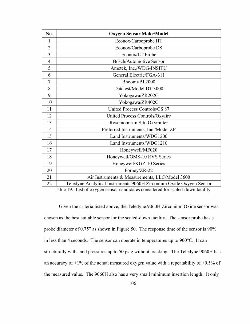
106

No. Oxygen Sensor Make/Model

1 Econox/Carboprobe HT

2 Econox/Carboprobe DS 3 Econox/LT Probe

4 Bosch/Automotive Sensor 5 Ametek, Inc./WDG-INSITU

6 General Electric/FGA-311 7 Bhoomi/BI 2000

8 Datatest/Model DT 3000 9 Yokogawa/ZR202G

10 Yokogawa/ZR402G 11 United Process Controls/CS 87

12 United Process Controls/Oxyfire 13 Rosemount/In Situ Oxymitter

14 Preferred Instruments, Inc./Model ZP 15 Land Instruments/WDG1200

16 Land Instruments/WDG1210 17 Honeywell/MF020

18 Honeywell/GMS-10 RVS Series 19 Honeywell/KGZ-10 Series

20 Forney/ZR-22 21 Air Instruments & Measurements, LLC/Model 3600 22 Teledyne Analytical Instruments 9060H Zirconium Oxide Oxygen Sensor

Table 19. List of oxygen sensor candidates considered for scaled-down facility

Given the criteria listed above, the Teledyne 9060H Zirconium Oxide sensor was

chosen as the best suitable sensor for the scaled-down facility. The sensor probe has a

probe diameter of 0.75” as shown in Figure 50. The response time of the sensor is 90%

in less than 4 seconds. The sensor can operate in temperatures up to 900°C. It can

structurally withstand pressures up to 50 psig without cracking. The Teledyne 9060H has

an accuracy of ±1% of the actual measured oxygen value with a repeatability of ±0.5% of

the measured value. The 9060H also has a very small minimum insertion length. It only

107

requires that the sensing element which is located at the tip of the probe be exposed to the

sample gas to be analyzed.

Figure 50. Schematic of Teledyne Series 9060 Zirconium Oxide Oxygen Sensor [37]

Non-intrusive methods for measuring oxygen concentration were also explored

and will be used in the current design. This can be done through planar laser-induced

108

fluorescence. With the current window design that allows one to look into the vessel,

oxygen concentration can be measured using a Nd:Yag Pulsed Laser set to a wavelength

of 266 nm while seeding the air with acetone. The images are then captured on a high

speed electronic camera and processed on the computer. Measurements of this type have

been up to temperatures of 1000 K.

Local Velocity

To make local velocity measurements, traditional methods were considered such

as pitot tubes and thermal anemometers. However, due to the low-flow conditions, the

resulting dynamics pressure will not be sufficiently large that velocity can be accurately

measured. Furthermore, due to the high temperature and transient concentration, thermal

anemometry becomes very difficult, if not impractical, to implement. Therefore, the best

option to measure local velocity conditions for high temperature, low-flow conditions is

particle image velocimetry.

Particle image velocimetry (PIV) tracks the motion of seeding particles that are

embedded in the flow with a laser and camera system. This is similar to what is done in

planar laser-induced fluorescence (PLIF) except with PIV the camera is tracking the

reflection of the laser beam from the seeding particles. During PLIF, there’s actually a

molecular excitation so the wavelength of light that is observed by the camera is different

than the wavelength of the laser. The seeding particles that are used for PIV are titanium

dioxide. These have an exceptionally high melting point approximately 1830°C so they

are suitable for this application.

109

Conclusion

The concept for a modified 1/8th geometric scaled-down facility has been

demonstrated. The scaled-down test facility is similar to the prototypic geometry in

terms of hydraulic resistance. In fact, on average, the non-dimensional resistance number

of the scaled-down facility deviates 2.81% in terms of relative accuracy from the non-

dimensional resistance number of the prototypic design while the non-dimensional

Froude number is matched perfectly.

A heat transfer characterization of the scaled-down facility is performed and

compared against the prototypic case. Utilizing different boundary conditions of a one-

dimensional fin analysis, the mole fraction of air was varied as well its far-field

temperature. The results demonstrate that the heat transfer coefficient varies from about

3-12 W/(m2·K) for the prototype geometry and from 5-15 W/(m2·K) for the scaled-down

geometry. Since the heat transfer coefficients vary over a small interval, despite different

boundary conditions and parameter values, the natural circulation phenomenology of

each geometric case will be preserved. Moreover, the range of heat transfer coefficients

for the prototype and scaled-down geometries are very similar. This means that the heat

transfer coefficient in the prototype system and the scaled-down system will be close

enough to each other during the course of an event that the basic natural circulation

phenomenology will be preserved. This ensures that a high degree of heat transfer

similarity will be maintained.

In addition to a heat transfer characterization of the scaled-down facility,

calculations were performed to determine the operational heating power of shell/heater

110

system and to validate the lumped capacitance approximation. The calculations show

that with a heater power of 125 W the surface temperature distribution of the rod is

closely matched to the surface temperature distribution of a scaled-down solid rod and a

prototypic support column. Moreover, the average radial heat flux of the shell/heater

system is closely matched to the prototypic and scaled-down rods when the heater power

is 0 W. In the course of this analysis, an overall time scale was provided which is

dependent on the density-driven stratified flow and hot plenum natural circulation

phenomena. The overall time scale is 16.07 s for the prototypic case and 5.67 s for the

scaled-down case.

A containment free volume (V = 1 m3) was determined to house the scaled-down

facility. With the containment free volume known, initial vessel pressures to preserve the

air-to-helium mole ratio (P = 40 psig) and mixed mean temperature (P = 34.2 psig) of the

prototype case were calculated. The initial stages of the blowdown were studied. It was

found that in both types of geometry that the duration of the blowdown is negligible

when compared to the total time scale of the air-ingress accident, but that helium

temperature dropped appreciably. This issue was resolved by maintaining similarity of

the non-dimensional Froude number over the temperature range of interest.

Vessel design drawings have been provided as well as the rationale for the current

design. The type of instrumentation (temperature, pressure, velocity, and concentration)

and the sensors’ locations were provided. The location of these sensors was determined,

in large part, by the computational fluid dynamic studies available in the literature as well

as those being performed at the author’s institution.

111

112

References

1. C.H. Oh, C. Davis, L. Siefken, R. Moore, H.C. No, J. Kim, G.C. Park, J.C. Lee, and W.R. Martin, “Development of Safety Analysis Codes and Experimental Validation for a Very High Temperature Gas-Cooled Reactor,” INL/EXT-06-01362, Idaho National Laboratory Report, March 2006

2. M. Hishida, T. Takeda, “Study on air ingress during an early stage of a primary-pipe rupture accident of a high-temperature gas-cooled reactor,” Nuclear Engineering and Design, 126, 175 (1991)

3. T. Takeda, M. Hishida, “Studies on molecular diffusion and natural convection in a multicomponent gas system,” International Journal of Heat and Mass Transfer, 39, 527 (1996)

4. E.S. Kim, H.C. No, B. Kim, C.H. Oh, “Estimation of graphite density and mechanical strength variation of VHTR during air-ingress accident,” Nuclear Engineering and Design, 238, 837 (2008)

5. H.C. No, H.S. Kim, J. Kim, C.H. Oh, L. Siefken, C. Davis, “Multi-component diffusion analysis and assessment of GAMMA code and improved RELAP 5 code,” Nuclear Engineering and Design, 237, 997 (2008)

6. E.S. Kim, C.H. Oh, R. Schultz, D. Petti, “Analysis on the Density Driven Air-Ingress Accident in VHTRs,” Transactions of the American Nuclear Society, 99, 2008

7. C.H. Oh, E.S. Kim, H.C. No, N.Z. Cho, “Experimental Validation of Stratified Flow Phenomena, Graphite Oxidation, and Mitigation Strategies of Air Ingress Accident,” FY08 Report, Idaho National Laboratory, INL/EXT-08-14840, December 2008

8. C.H. Oh, E.S. Kim, H.C. No, N.Z. Cho, “Experimental Validation of Stratified Flow Phenomena, Graphite Oxidation, and Mitigation Strategies of Air Ingress Accident,” FY09 Report, Idaho National Laboratory, INL/EXT-09-16465, December 2009

9. C.H. Oh, Hyung S. Kang, Eung S. Kim, "Air-ingress analysis: Part 2 – Computational fluid dynamic models," Nuclear Engineering and Design, 241, 213 (2011)

10. C.H. Oh, Eung S. Kim, "Air-ingress analysis: Part 1 Theoretical approach," Nuclear Engineering and Design, 241, 203 (2011)

11. N. Kodochigov, “Neutronic features of the GT-MHR reactor,” Nuclear Engineering and Design, 222, 161 (2002)

113

12. “NGNP Point Design – Results of the Initial Neutronics and Thermal-Hydraulic Assessments During FY-03,” INEEL/EXT-03-00870, September 2003

13. “VHTR – Survey of Materials Research and Development Needs to Support Early Deployment,” INEEL/EXT-03-00141, January 2003

14. A.J. Neylan, A. Shenoy, F.A. Silady, T.D. Dunn, “GT-MHR Design, Performance and Safety,” General Atomics, Inc. GA-A-21924, November 1994

15. N. Tak, M. Kim, W.J. Lee, “Numerical investigation of a heat transfer within the prismatic fuel assembly of a very high temperature reactor,” Annals of Nuclear Energy, 35, (2008)

16. K.G. Condie, “Development of an Experiment for Measuring Flow Phenomena Occurring in a Lower Plenum for VHTR CFD Assessment,” INL/EXT-05-00603, September 2005

17. S.M. Mohsin Reza, “Design of an Alternative Coolant Inlet Flow Configuration for the Modular Helium Reactor,” ICAPP 2006, June 2006

18. General Atomics, 1996, "Gas Turbine-Modular Helium Reactor (GT-MHR) Conceptual Design Description Report," GA Project No. 7658, 910720 Revision 1, July 1996

19. K.N. Iyer, A. Kadengal, “Scaling of Natural Circulation Boiling Systems,” Proceedings of ASME Summer Heat Transfer Conference, July 21-23, 2003, Las Vegas, Nevada, USA

20. M. Ishii, “Scaling Laws for Thermal-Hydraulic System Under Single Phase and Two-Phase Natural Circulation,” Nuclear Engineering and Design, 81, 411 (1984)

21. P.K. Vijayan, H. Austregesilo, “Scaling laws for single-phase natural circulation loops,” Nuclear Engineering and Design, 152, 331 (1994)

22. P.K. Vijayan, “Experimental observations on the general trends of the steady state and stability behavior of single-phase natural circulation loops,” Nuclear Engineering and Design, 215, 139 (2002)

23. P.K. Vijayan, M.R. Gartia, G.S.S.P. Rao, D.S. Pilkhwal, D. Saha, “Steady State Behaviour of Single-Phase and Two-Phase Natural Circulation Loops,” 2nd RCM on the IAEA CRP on ‘Natural Circulation phenomena, modeling, and reliability of passive systems that utilize natural circulation,’ August 29 – September 02, 2005, Corvalis, OR, USA

114

24. A.I. Zografos, W.A. Martin, J.E. Sunderland, “Equations of properties as a function of temperature for seven fluids,” Computer Methods in Applied Mechanics and Engineering, 61, 177 (1987)

25. G. Latini, G. Passerini, F. Polonara, “Thermophysical Properties of Greenhouse Gases Thermal Conductivity and Dynamic Viscosity as Function of Temperature and Pressure,” Energy Conversion Management, 37 Nos. 6-8, 1291 (1996)

26. H. Petersen, “The Properties of Helium: Density, Specific Heats, Viscosity, and Thermal Conductivity at Pressures from 1 to 100 bar and from Room Temperature to about 1800 K”, Danish Atomic Energy Commission, Report No. 224, September 1970

27. J.N. Reyes Jr., J.T. Groome, B.G. Woods, B. Jackson and T.D. Marshall, "Scaling analysis for the high temperature Gas Reactor Test Section (GRTS)," Nuclear Engineering and Design, 240, 397 (2010)

28. J.P. Abraham, E.M. Sparrow, W.J. Minkowycz, “Internal-flow Nusselt numbers for the low-Reynolds-number end of the laminar-to-turbulent transition regime,” International Journal of Heat and Mass Transfer, 54, 584 (2011)

29. I.E. Idelchik, Handbook of Hydraulic Resistance, 2nd Edition, 1986, Hemisphere Publishing Corporation

30. N.E. Todreas and M.S. Kazimi, Nuclear Systems I: Thermal Hydraulic Fundamentals, 1st Edition Second Printing, Taylor & Francis

31. A. Banerjee and M. Andrews, “A Convection Heat Transfer Correlation for a Binary Air-Helium Mixture at Reynolds Number,” Journal of Heat Transfer, 129, 1494 (2007)

32. T. Maruyama, T. Kaito, S. Onose, I. Shibahara, “Change in physical properties of high density isotropic graphites irradiated in the “JOYO” fast reactor,” Journal of Nuclear Material, 225, 267 (1995)

33. J.L. Xia, B.L. Smith, G. Yadigaroglu, “A Simplified Model for Depressurization of Gas-filled Pressure Vessels,” International Communications of Heat and Mass Transfer, 20, 653 (1993)

34. Conax® Technologies, http://www.conaxtechnologies.com 35. Rayotek Scientific Inc., http://www.rayotek.com/tech-specs/specs_pdf.htm

36. Honeywell Specification and Model Selection Guide for ST 3000 Smart Transmitter,

34-ST-03-67

115

37. Teledyne Analytical Instruments, http://www.teledyne-ai.com/pdf/9060.pdf

38. D.J. Arcilesi, T. Ham, X.Sun, R.N. Christensen, C.H. Oh, “Density Driven Air

Ingress and Hot Plenum Natural Circulation for a VHTR,” Transactions of the American Nuclear Society, 105, 990 (2011)

116

Appendix A: The Complete Results from One-dimensional Support Column Fin

Analysis

These figures represent the complete set of results for the one-dimensional

support column heat transfer fin analysis that was performed in Chapter 2. The first set

of figures is for the prototype geometry (Figure 51 - Figure 60) while the second set of

figures is for the scaled-down geometry (Figure 61 - Figure 70). The Biot number, the

thermal time constant, the boundary later thickness, the average heat transfer coefficient,

and average Rayleigh number are plotted against the far-field temperature and the air

mole fraction while being parameterized by the other in a given figure.

117

Prototype Geometry and Specifications

Figure 51. Average Biot number v. far-field temperature for prototype geometry

Figure 52. Average Biot number v. air mole fraction for prototype geometry

0

0.001

0.002

0.003

0.004

0.005

0.006

0.007

0 100 200 300 400 500

Average

 Biot Number

Far‐field Temperature, T∞ (°C)

Average Biot Number v. Far‐field Temperature (Prototype; Ttop = 850°C)

100% He

90% He/10% Air

80% He/20% Air

70% He/80% Air

60% He/40% Air

50% He/50% Air

40% He/60% Air

30% He/70% Air

20% He/80% Air

10% He/ 90% Air

100% Air

0

0.001

0.002

0.003

0.004

0.005

0.006

0.007

0 0.2 0.4 0.6 0.8 1

Average

 Biot Number

Air Mole Fraction

Average Biot Number v. Air Mole Fraction (Prototype; Ttop = 850°C)

25 C

50 C

100 C

150 C

170 C

200 C

250 C

300 C

350 C

400 C

450 C

500 C

118

Figure 53. Average thermal time constant v. far-field temperature for prototype geometry

Figure 54. Average thermal time constant v. air mole fraction for prototype geometry

0

10000

20000

30000

40000

50000

60000

0 100 200 300 400 500Average

 Therm

al Tim

e Constan

t (s)

Far‐field Temperature, T∞(°C)

Average Thermal Time Constant v. Far‐field Temperature (Prototype; Ttop = 850°C)

100% He

90% He/10% Air

80% He/20% Air

70% He/30% Air

60% He/ 40% Air

50% He/50% Air

40% He/60% Air

30% He/70% Air

20% He/80% Air

10% He/90% Air

100% Air

0

10000

20000

30000

40000

50000

60000

0 0.2 0.4 0.6 0.8 1

Average

 Therm

al Tim

e Constan

t (s)

Air Mole Fraction

Average Thermal Time Constant v. Air Mole Fraction (Prototype; Ttop = 850°C) 25 C

50 C

100 C

150 C

170 C

200 C

250 C

300 C

350 C

400 C

450 C

500 C

119

Figure 55. Average boundary layer thickness v. far-field temperature for prototype geometry

Figure 56. Average boundary layer thickness v. far-field temperature for prototype geometry

0

0.02

0.04

0.06

0.08

0.1

0.12

0.14

0.16

0.18

0 100 200 300 400 500Average

 Boundary Layer Th

ickn

ess (m) 

(Top of Support Column)

Far‐field Temperature, T∞(°C)

Average Boundary Layer Thickness v. Far‐Field Temperature (Prototype; Ttop = 850°C)

100% Helium

90% He/10% Air

80% He/20% Air

70% He/30% Air

60% He/40% Air

50% He/50% Air

40% He/60% Air

30% He/70% Air

20% He/80% Air

10% He/90% Air

100% Air

0

0.02

0.04

0.06

0.08

0.1

0.12

0.14

0.16

0.18

0 0.2 0.4 0.6 0.8 1Average

 Boundary Layer Th

ickn

ess (m)                 

(Tope of Support Column)

Air Mole Fraction

Average Boundary Layer Thickness v. Air Mole Fraction (Prototype; Ttop = 850°C)

25 C

50 C

100 C

150 C

170 C

200 C

250 C

300 C

350 C

400 C

450 C

500 C

120

Figure 57. Average heat transfer coefficient v. far-field temperature for prototype geometry

Figure 58. Average heat transfer coefficient v. far-field temperature for prototype geometry

2

4

6

8

10

12

14

16

0 100 200 300 400 500Average

 Heat Transfer Coefficient (W

/(m

2*K

))

Far‐field Temperature , T∞(°C)

Average Heat Transfer Coefficient v. Far‐field Temperature (Prototype; Ttop = 850°C) 

100% He

90% He/10% Air

80% He/20% Air

70% He/30% Air

60% He/40% Air

50% He/50% Air

40% He/60% Air

30% He/70% Air

20% He/80% Air

10% He/90% Air

100% Air

2

4

6

8

10

12

14

16

0 0.2 0.4 0.6 0.8 1

Average

 Heat Transfer Coefficient (W

/(m

2*K

))

Air Mole Fraction

Average Heat Transfer Coefficient v. Air Mole Fraction (Prototype; Ttop = 850°C)

25 C

50 C

100 C

150 C

170 C

200 C

250 C

300 C

350 C

400 C

450 C

500 C

121

Figure 59. Average Rayleigh number v. far-field temperature for prototype geometry

Figure 60. Average Rayleigh number v. air mole fraction for prototype geometry

1.00000E+07

1.00000E+08

1.00000E+09

1.00000E+10

1.00000E+11

1.00000E+12

0 100 200 300 400 500

Average

 Rayleigh Number

Far‐field Temperature, T∞ (°C)

Average Rayleigh Number v. Far‐field Temperature (Prototype; Ttop = 850°C)

100% He

90% He/10% Air

80% He/20% Air

70% He/30% Air

60% He/40% Air

50% He/50% Air

40% He/60% Air

30% He/70% Air

20% He/80% Air

10% He/90% Air

100% Air

1.00000E+08

1.00000E+09

1.00000E+10

1.00000E+11

1.00000E+12

0 0.2 0.4 0.6 0.8 1

Average

 Rayleigh Number

Air Mole Fraction

Average Rayleigh Number v. Air Mole Fraction (Prototype; Ttop = 850°C)

25 C

50 C

100 C

150 C

170 C

200 C

250 C

300 C

350 C

400 C

450 C

500 C

122

Scaled-down Geometry and Specifications

Figure 61. Average Biot number v. far-field temperature for scaled-down geometry

Figure 62. Average Biot number v. air mole fraction for scaled-down geometry

0.0005

0.0007

0.0009

0.0011

0.0013

0.0015

0.0017

0.0019

0.0021

0.0023

0.0025

0 100 200 300 400 500

Average

 Biot Number

Far‐field Temperature, T∞ (°C)

Average Biot Number v. Far‐field Temperature (Scaled‐down; Ttop = 750°C)

100% He

90% He/10% Air

80% He/20% Air

70% He/30% Air

60% He/40% Air

50% He/50% Air

40% He/60% Air

30% He/70% Air

20% He/80% Air

10% He/90% Air

100% Air

0.0005

0.0007

0.0009

0.0011

0.0013

0.0015

0.0017

0.0019

0.0021

0.0023

0.0025

0 0.2 0.4 0.6 0.8 1

Average

 Biot Number

Air Mole Fraction

Average Biot Number v. Air Mole Fraction (Scaled‐down; Ttop = 750°C) 25 C

50 C

100 C

150 C

170 C

200 C

250 C

300 C

350 C

400 C

450 C

500 C

123

Figure 63. Average thermal time constant v. far-field temperature for scaled-down geometry

Figure 64. Average thermal time constant v. air mole fraction for scaled-down geometry

2000

3000

4000

5000

6000

7000

8000

9000

0 100 200 300 400 500

Average

 Therm

al Tim

e Constan

t (s)

Far‐field Temperature, T∞(°C)

Average Thermal Time Constant v. Far‐field Temperature (Scaled‐down; Ttop = 750°C)

100% He

90% He/10% Air

80% He/20% Air

70% He/30% Air

60% He/40% Air

50% He/50% Air

40% He/60% Air

30% He/70% Air

20% He/80% Air

10% He/90% Air

100% Air

0

1000

2000

3000

4000

5000

6000

7000

8000

9000

0 0.2 0.4 0.6 0.8 1

Average

 Therm

al Tim

e Constan

t (s)

Air Mole Fraction

Average Thermal Time Constant v. Air Mole Fraction (Scaled‐down; Ttop = 750°C)

25 C

50 C

100 C

150 C

170 C

200 C

250 C

300 C

350 C

400 C

124

Figure 65. Average boundary layer thickness v. far-field temperature for scaled-down geometry

Figure 66. Average boundary layer thickness v. air mole fraction for scaled-down geometry

0

0.02

0.04

0.06

0.08

0.1

0.12

0 100 200 300 400 500Average

 Boundary Layer Th

ickn

ess (m)  

(Top of Support Column)

Far‐field Temperature, T∞(°C)

Average Boundary Layer Thickness v. Far‐field Temperature (Scaled‐down; Ttop = 750°C)

100% He

90% He/10% Air

80% He/20% Air

70% He/30% Air

60% He/40% Air

50% He/50% Air

40% He/60% Air

30% He/70% Air

20% He/80% Air

10% He/90% Air

100% Air

0

0.02

0.04

0.06

0.08

0.1

0.12

0 0.2 0.4 0.6 0.8 1

Average

 Boundary Layer Th

ickn

ess (m)                       

(Top of Support Column)

Air Mole Fraction

Average Boundary Layer Thickness v. Air Mole Fraction (Scaled‐down; Ttop = 750°C)

25 C

50 C

100 C

150 C

170 C

200 C

250 C

300 C

350 C

400 C

450 C

500 C

125

Figure 67. Average heat transfer coefficient v. far-field temperature for scaled-down geometry

Figure 68. Average heat transfer coefficient v air mole fraction for scaled-down geometry

2

4

6

8

10

12

14

16

0 100 200 300 400 500

Average

 Heat Transfer Coefficient (W

/(m

2*K

))

Far‐field Temperature , T∞(°C)

Average Heat Transfer Coefficient v. Far‐field Temperature (Scaled‐down; Ttop = 750°C) 

100% He

90% He/10% Air

80% He/20% Air

70% He/30% Air

60% He/40% Air

50% He/50% Air

40% He/60% Air

30% He/70% Air

20% He/80% Air

10% He/90% Air

100% Air

2

4

6

8

10

12

14

16

0 0.2 0.4 0.6 0.8 1Average

 Heat Transfer Coefficient 

(W/(m

2*K

))

Air Mole Fraction

Average Heat Transfer Coefficient v. Air Mole Fraction (Scaled‐down; Ttop = 750°C) 25 C

50 C

100 C

150 C

170 C

200 C

250 C

300 C

350 C

400 C

450 C

500 C

126

Figure 69. Average Rayleigh number v. far-field temperature for scaled-down geometry

Figure 70. Average Rayleigh number v. air mole fraction for scaled-down geometry

1.00E+05

1.00E+06

1.00E+07

1.00E+08

1.00E+09

0 100 200 300 400 500

Average

 Rayleigh Number

Far‐field Temperature, T∞ (°C)

Average Rayleigh Number v. Far‐field Temperature (Scaled‐down; Ttop = 750°C)

100% He

90% He/10% Air

80% He/20% Air

70% He/30% Air

60% He/40% Air

50% He/50% Air

40% He/60% Air

30% He/70% Air

20% He/80% Air

10% He/90% Air

100% Air

1.00E+05

1.00E+06

1.00E+07

1.00E+08

1.00E+09

0 0.2 0.4 0.6 0.8 1

Average

 Rayleigh Number

Air Mole Fraction

Average Rayleigh Number v. Air Mole Fraction (Scaled‐down; Ttop = 750°C)

25 C

50 C

100 C

150 C

170 C

200 C

250 C

300 C

350 C

400 C

450 C

500 C

127

Appendix B: MATLAB Codes

MATLAB code for heat transfer characteristics of a support column using a one-dimensional fin analysis with fixed temperature (Dirichlet) boundary conditions

%%% Heat Transfer Coefficients, Biot Numbers, and Transient Conduction Time %%% Scales for Prototype/Scaled-Down VHTR Support Columns: 1-D Calculation %%% Dirichlet Boundary Conditions %%% Binary Mixture: Air/Helium clc; clear all; close all format long % Input T_inf = 50; % units = [C]; far-field temperature y_a = 1; % unitless; air mole fraction y_he = 1 - y_a; % unitless; helium mole fraction H = 2.84; % units = [m]; prototype rod height D = 0.212; % units = [m]; prototype rod diameter %H = 0.3556; % units = [m]; scaled-down rod height %D = 0.055; % units = [m]; scaled-down rod diameter T_o = 750; % units = [C]; upper-boundary temperature - top of the rod T_H = 490; % units = [C]; lower-boundary temperature - bottom of the rod % Initial Temperature and Pressure Tw = (T_o + T_H)/2; % initial average wall temp; units = [C] P = 1.01325; % units = [bar] % Constants g = 9.81; % units = [m/s^2]; acceleration of gravity M_he = 4.002602; % units = [g/mol]; Helium molecular weight M_a = 28.9644; % units = [g/mol]; Air molecular weight

128

mf_he = (y_he*M_he)/(y_he*M_he + y_a*M_a); % unitless; Helium mass fraction mf_a = 1 - mf_he; % unitless; Air mass fraction R = 8.314462175; % units = [J/mol/K]; Universal Gas Constant R_a = 1000*R/M_a; % units = [J/kg/K]; Specific Gas Constant for Air R_he = 1000*R/M_he; % units = [J/kg/K]; Specific Gas Constant for He tol = 1e-12; % error tolerance res = 0.1; % error residual iter = 0; % iteration count while res > tol T = (Tw + T_inf)/2; % Helium Thermo-physical Properties mu_he = 3.674e-7*(T + 273.15)^0.7; % Dynamic Viscosity; units = [kg/(m*s)] rho_he = 48.14*P/(T + 273.15)*(1 + 0.4446*P/(T + 273.15)^1.2)^-1; % Density; units = [kg/m^3] nu_he = mu_he/rho_he; % kinematic viscosity; momentum diffusivity; units = [m^2/s] kf_he = 2.682e-3*(1 + 1.123e-3*P)*(T + 273.15)^(0.71*(1 - 2e-4*P)); % Fluid thermal conductivity; units = [W/(m*K)] cp_he = 5193; % units = [J/kg/K]; Specific Heat Capacity at Constant Pressure % Air Thermo-physical Properties mu_a = 2.5914e-15*(T + 273.15)^3 - 1.4346e-11*(T + 273.15)^2 +... 5.0523e-8*(T + 273.15) + 4.1130e-6; % Dynamic Viscosity; units = [Pa*s] rho_a = 345.57*((T + 273.15) - 2.6884)^-1; % Density; units = [kg/m^3] nu_a = mu_a/rho_a; % kinematic viscosity; momentum diffusivity; units = [m^2/s] kf_a = 3.42253617e-4 + 9.8497252e-5*(T + 273.15) - 4.88240e-8*(T + 273.15)^2 +... 1.7542e-11*(T + 273.15)^3; % Air thermal conductivity; units = [W/(m*K)] cp_a = 1000*(1.3864e-13*(T + 273.15)^4 - 6.4747e-10*(T + 273.15)^3 +... 1.0234e-6*(T + 273.15)^2 - 4.3282e-4*(T +273.15) + 1.0613); % units = [J/kg/K]; % Specific Heat Capacity at Constant Pressure % Air-Helium Mixture Thermo-physical Properties rho = y_he*rho_he + y_a*rho_a; % units = [kg/m^3]; Mixture Density phi_a = (1 + (mu_a/mu_he)^(1/2)*(M_he/M_a)^(1/4))^2*(8*(1 + M_a/M_he))^(1/2);

129

phi_he = (1 + (mu_he/mu_a)^(1/2)*(M_a/M_he)^(1/4))^2*(8*(1 + M_he/M_a))^(1/2); mu = mu_a*(1 + y_he/y_a*phi_a)^(-1) + mu_he*(1 + y_a/y_he*phi_he)^(-1); % units = [Pa*s]; Mixture Dynamic Viscosity nu = mu/rho; % units = [m^2/s]; Kinematic Viscosity P_a = 0.115 + 0.354*(cp_a/R_a); P_he = 0.115 + 0.354*(cp_he/R_he); phip_a = 1.065*(1 + ((kf_a*P_he)/(kf_he*P_a))^(1/2)*(M_he/M_a)^(1/4))^2*... (8*(1 + M_a/M_he))^(-1/2); phip_he = 1.065*(1 + ((kf_he*P_a)/(kf_a*P_he))^(1/2)*(M_a/M_he)^(1/4))^2*... (8*(1 + M_he/M_a))^(-1/2); kf = kf_a*(1 + y_he/y_a*phip_a)^(-1) + kf_he*(1 + y_a/y_he*phip_he)^(-1); % units = [W/m/K]; Mixture Thermal Conductivity cp = mf_a*cp_a + mf_he*cp_he; % units = [J/kg/K]; Mixture Specific Heat at Constant Pressure % Non-Dimensional Numbers Pr = mu*cp/kf; % Prandtl Number; dimensionless Gr = g*1/(T + 273.15)*(Tw - T_inf)*H^3/nu^2; % Grashof Number; dimensionless Ra = Pr*Gr; % Rayleigh Number; dimensionless if Ra > 1e9 Nu = 0.10*Ra^(1/3); else Nu = 0.59*Ra^(1/4); end h = Nu*kf/H; % heat transfer coefficient; units = [W/m^2/K] % Rod Thermo-physical Properties ks = 3e-8*Tw^3 - 1e-5*Tw^2 - 0.0612*Tw + 125.56; % unirradiated rod thermal conductivity; units = [W/m/K] cps = 9e-7*Tw^3 - 0.0027*Tw^2 + 3.0203*Tw + 643.24; % rod specific heat capacity; units = [J/(kg*K)] rhos = 1770; % rod density; units = [kg/m^3] m = (4*h/(D*ks))^(1/2); % units = [m^-1] Tw_new = (T_H + T_o - 2*T_inf)*(cosh(m*H) - 1)/(m*H*sinh(m*H)) + T_inf; % new average rod temp; units = [C] res = abs(Tw_new - Tw); Tw = Tw_new; iter = iter + 1;

130

end h Bi = h*D/(4*ks) Ra tau = rhos*D*cps/(4*h) BL = 3.93*Pr^(-1/2)*(0.952 + Pr)^(1/4)*Gr^(-1/4)*H % Boundary Layer Thickness; units = [m]

131

MATLAB code for heat transfer characteristics of a support column using a one-dimensional fin analysis with mixed boundary conditions

%%% Heat Transfer Coefficients, Biot Numbers, and Transient Conduction Time %%% Scales for Prototype/Scaled-Down VHTR Support Columns: 1-D Calculation %%% Mixed Boundary Conditions %%% Binary Mixture: Air/Helium clc; clear all; close all format long % Input T_inf = 50; % units = [C]; far-field temperature y_a = 1; % unitless; helium mole fraction y_he = 1 - y_a; % unitless; air mole fraction H = 2.84; % units = [m]; prototype rod height D = 0.212; % units = [m]; prototype rod diameter %H = 0.3556; % units = [m]; scaled-down rod height %D = 0.055; % units = [m]; scaled-down rod diameter T_o = 750; % units = [C]; upper-boundary temperature - top of the rod T_H = 490; % units = [C]; lower-boundary temperature - bottom of the rod % Initial Temperature and Pressure Tw = (T_o + T_H)/2; % initial average wall temp; units = [C] P = 1.01325; % units = [bar] % Constants g = 9.81; % units = [m/s^2]; acceleration of gravity M_he = 4.002602; % units = [g/mol]; Helium molecular weight M_a = 28.9644; % units = [g/mol]; Air molecular weight mf_he = (y_he*M_he)/(y_he*M_he + y_a*M_a); % unitless; Helium mass fraction mf_a = 1 - mf_he; % unitless; Air mass fraction R = 8.314462175; % units = [J/mol/K]; Universal Gas Constant R_a = 1000*R/M_a; % units = [J/kg/K]; Specific Gas Constant for Air R_he = 1000*R/M_he; % units = [J/kg/K]; Specific Gas Constant for He

132

tol = 1e-12; % error tolerance res = 0.1; % error residual iter = 0; % iteration count while res > tol T = (Tw + T_inf)/2; % Helium Thermo-physical Properties mu_he = 3.674e-7*(T + 273.15)^0.7; % Dynamic Viscosity; units = [kg/(m*s)] rho_he = 48.14*P/(T + 273.15)*(1 + 0.4446*P/(T + 273.15)^1.2)^-1; % Density; units = [kg/m^3] nu_he = mu_he/rho_he; % kinematic viscosity; momentum diffusivity; units = [m^2/s] kf_he = 2.682e-3*(1 + 1.123e-3*P)*(T + 273.15)^(0.71*(1 - 2e-4*P)); % Fluid thermal conductivity; units = [W/(m*K)] cp_he = 5193; % units = [J/kg/K]; Specific Heat Capacity at Constant Pressure % Air Thermo-physical Properties mu_a = 2.5914e-15*(T + 273.15)^3 - 1.4346e-11*(T + 273.15)^2 +... 5.0523e-8*(T + 273.15) + 4.1130e-6; % Dynamic Viscosity; units = [Pa*s] rho_a = 345.57*((T + 273.15) - 2.6884)^-1; % Density; units = [kg/m^3] nu_a = mu_a/rho_a; % kinematic viscosity; momentum diffusivity; units = [m^2/s] kf_a = 3.42253617e-4 + 9.8497252e-5*(T + 273.15) - 4.88240e-8*(T + 273.15)^2 +... 1.7542e-11*(T + 273.15)^3; % Air thermal conductivity; units = [W/(m*K)] cp_a = 1000*(1.3864e-13*(T + 273.15)^4 - 6.4747e-10*(T + 273.15)^3 +... 1.0234e-6*(T + 273.15)^2 - 4.3282e-4*(T +273.15) + 1.0613); % units = [J/kg/K]; % Specific Heat Capacity at Constant Pressure % Air-Helium Mixture Thermo-physical Properties rho = y_he*rho_he + y_a*rho_a; % units = [kg/m^3]; Mixture Density phi_a = (1 + (mu_a/mu_he)^(1/2)*(M_he/M_a)^(1/4))^2*(8*(1 + M_a/M_he))^(1/2); phi_he = (1 + (mu_he/mu_a)^(1/2)*(M_a/M_he)^(1/4))^2*(8*(1 + M_he/M_a))^(1/2); mu = mu_a*(1 + y_he/y_a*phi_a)^(-1) + mu_he*(1 + y_a/y_he*phi_he)^(-1); % units = [Pa*s]; Mixture Dynamic Viscosity nu = mu/rho; % units = [m^2/s]; Kinematic Viscosity

133

P_a = 0.115 + 0.354*(cp_a/R_a); P_he = 0.115 + 0.354*(cp_he/R_he); phip_a = 1.065*(1 + ((kf_a*P_he)/(kf_he*P_a))^(1/2)*(M_he/M_a)^(1/4))^2*... (8*(1 + M_a/M_he))^(-1/2); phip_he = 1.065*(1 + ((kf_he*P_a)/(kf_a*P_he))^(1/2)*(M_a/M_he)^(1/4))^2*... (8*(1 + M_he/M_a))^(-1/2); kf = kf_a*(1 + y_he/y_a*phip_a)^(-1) + kf_he*(1 + y_a/y_he*phip_he)^(-1); % units = [W/m/K]; Mixture Thermal Conductivity cp = mf_a*cp_a + mf_he*cp_he; % units = [J/kg/K]; Mixture Specific Heat at Constant Pressure % Non-Dimensional Numbers Pr = mu*cp/kf; % Prandtl Number; dimensionless Gr = g*1/(T + 273.15)*(Tw - T_inf)*H^3/nu^2; % Grashof Number; dimensionless Ra = Pr*Gr; % Rayleigh Number; dimensionless if Ra > 1e9 Nu = 0.10*Ra^(1/3); else Nu = 0.59*Ra^(1/4); end h = Nu*kf/H; % heat transfer coefficient; units = [W/m^2/K] % Rod Thermo-physical Properties ks = 3e-8*Tw^3 - 1e-5*Tw^2 - 0.0612*Tw + 125.56; % unirradiated rod thermal conductivity; units = [W/m/K] cps = 9e-7*Tw^3 - 0.0027*Tw^2 + 3.0203*Tw + 643.24; % rod specific heat capacity; units = [J/(kg*K)] rhos = 1770; % rod density; units = [kg/m^3] m = (4*h/(D*ks))^(1/2); % units = [m^-1] Tw_new = (T_o - T_inf)/(m*H)*tanh(m*H) + T_inf; % new average rod temp; units = [C] res = abs(Tw_new - Tw); Tw = Tw_new; iter = iter + 1; end h Bi = h*D/(4*ks) Ra tau = rhos*D*cps/(4*h)

134

BL = 3.93*Pr^(-1/2)*(0.952 + Pr)^(1/4)*Gr^(-1/4)*H % Boundary Layer Thickness; units = [m]

135

MATLAB code for heat transfer characteristics of a support column using a one-dimensional fin analysis with constant wall temperature

%%% Heat Transfer Coefficients, Biot Numbers, and Transient Conduction Time %%% Scales for Prototype/Scaled-Down VHTR Support Columns: 1-D Calculation %%% Constant Wall Temperature %%% Binary Mixture: Air/Helium clc; clear all; close all format long % Input T_inf = 50; y_a = 1; % unitless; air mole fraction y_he = 1 - y_a; % unitless; helium mole fraction H = 2.84; % units = [m]; prototype rod height D = 0.212; % units = [m]; prototype rod diameter %H = 0.3556; % units = [m]; scaled-down rod height %D = 0.055; % units = [m]; scaled-down rod diameter % Initial Temperature and Pressure Tw = 750; % initial average wall temp; units = [C] P = 1.01325; % units = [bar] % Constants g = 9.81; % units = [m/s^2]; acceleration of gravity M_he = 4.002602; % units = [g/mol]; Helium molecular weight M_a = 28.9644; % units = [g/mol]; Air molecular weight mf_he = (y_he*M_he)/(y_he*M_he + y_a*M_a); % unitless; Helium mass fraction mf_a = 1 - mf_he; % unitless; Air mass fraction R = 8.314462175; % units = [J/mol/K]; Universal Gas Constant R_a = 1000*R/M_a; % units = [J/kg/K]; Specific Gas Constant for Air R_he = 1000*R/M_he; % units = [J/kg/K]; Specific Gas Constant for He iter = 0; % iteration count

136

T = (Tw + T_inf)/2; % Helium Thermo-physical Properties mu_he = 3.674e-7*(T + 273.15)^0.7; % Dynamic Viscosity; units = [kg/(m*s)] rho_he = 48.14*P/(T + 273.15)*(1 + 0.4446*P/(T + 273.15)^1.2)^-1; % Density; units = [kg/m^3] nu_he = mu_he/rho_he; % kinematic viscosity; momentum diffusivity; units = [m^2/s] kf_he = 2.682e-3*(1 + 1.123e-3*P)*(T + 273.15)^(0.71*(1 - 2e-4*P)); % Fluid thermal conductivity; units = [W/(m*K)] cp_he = 5193; % units = [J/kg/K]; Specific Heat Capacity at Constant Pressure % Air Thermo-physical Properties mu_a = 2.5914e-15*(T + 273.15)^3 - 1.4346e-11*(T + 273.15)^2 +... 5.0523e-8*(T + 273.15) + 4.1130e-6; % Dynamic Viscosity; units = [Pa*s] rho_a = 345.57*((T + 273.15) - 2.6884)^-1; % Density; units = [kg/m^3] nu_a = mu_a/rho_a; % kinematic viscosity; momentum diffusivity; units = [m^2/s] kf_a = 3.42253617e-4 + 9.8497252e-5*(T + 273.15) - 4.88240e-8*(T + 273.15)^2 +... 1.7542e-11*(T + 273.15)^3; % Air thermal conductivity; units = [W/(m*K)] cp_a = 1000*(1.3864e-13*(T + 273.15)^4 - 6.4747e-10*(T + 273.15)^3 +... 1.0234e-6*(T + 273.15)^2 - 4.3282e-4*(T +273.15) + 1.0613); % units = [J/kg/K]; % Specific Heat Capacity at Constant Pressure % Air-Helium Mixture Thermo-physical Properties rho = y_he*rho_he + y_a*rho_a; % units = [kg/m^3]; Mixture Density phi_a = (1 + (mu_a/mu_he)^(1/2)*(M_he/M_a)^(1/4))^2*(8*(1 + M_a/M_he))^(1/2); phi_he = (1 + (mu_he/mu_a)^(1/2)*(M_a/M_he)^(1/4))^2*(8*(1 + M_he/M_a))^(1/2); mu = mu_a*(1 + y_he/y_a*phi_a)^(-1) + mu_he*(1 + y_a/y_he*phi_he)^(-1); % units = [Pa*s]; Mixture Dynamic Viscosity nu = mu/rho; % units = [m^2/s]; Kinematic Viscosity P_a = 0.115 + 0.354*(cp_a/R_a); P_he = 0.115 + 0.354*(cp_he/R_he); phip_a = 1.065*(1 + ((kf_a*P_he)/(kf_he*P_a))^(1/2)*(M_he/M_a)^(1/4))^2*... (8*(1 + M_a/M_he))^(-1/2);

137

phip_he = 1.065*(1 + ((kf_he*P_a)/(kf_a*P_he))^(1/2)*(M_a/M_he)^(1/4))^2*... (8*(1 + M_he/M_a))^(-1/2); kf = kf_a*(1 + y_he/y_a*phip_a)^(-1) + kf_he*(1 + y_a/y_he*phip_he)^(-1); % units = [W/m/K]; Mixture Thermal Conductivity cp = mf_a*cp_a + mf_he*cp_he; % units = [J/kg/K]; Mixture Specific Heat at Constant Pressure % Non-Dimensional Numbers Pr = mu*cp/kf; % Prandtl Number; dimensionless Gr = g*1/(T + 273.15)*(Tw - T_inf)*H^3/nu^2; % Grashof Number; dimensionless Ra = Pr*Gr; % Rayleigh Number; dimensionless if Ra > 1e9 Nu = 0.10*Ra^(1/3); else Nu = 0.59*Ra^(1/4); end h = Nu*kf/H; % heat transfer coefficient; units = [W/m^2/K] % Rod Thermo-physical Properties ks = 3e-8*Tw^3 - 1e-5*Tw^2 - 0.0612*Tw + 125.56; % unirradiated rod thermal conductivity; units = [W/m/K] cps = 9e-7*Tw^3 - 0.0027*Tw^2 + 3.0203*Tw + 643.24; % rod specific heat capacity; units = [J/(kg*K)] rhos = 1770; % rod density; units = [kg/m^3] % hold on % plot(T_inf,h,'*') % xlabel('Far-field Temperature (C)') % ylabel('Heat Transfer Coefficient (W/(m^2*K))') % title('Heat Transfer Coefficient v. Far-field Temperature (C)') %legend('100% Helium','10% Air/90% He','20% Air/80% He','30% Air/70% He',... % '40% Air/60% He','50% Air/50% He','60% Air/40% He','70% Air/30% He',... %'80% Air/20% He','90% Air/10% He','100% Air',-1) h Bi = h*D/(4*ks) Ra tau = rhos*D*cps/(4*h)

138

BL = 3.93*Pr^(-1/2)*(0.952 + Pr)^(1/4)*Gr^(-1/4)*H % Boundary Layer Thickness; units = [m]

139

MATLAB code for one-dimensional transient temperature distribution of prototypic and scaled-down support columns

%%% One-dimensional Transient Temperature Profile for prototypic and scaled-down VHTR Support Columns in Cylindrical Coordinates %%% Finite Difference Discretization; Explicit Time Marching Scheme clc; clear all; close all format long %R = 0.106; % units = [m]; Prototype Support Column Radius R = 0.0275; % units = [m]; Scaled-Down Support Column Radius N = 301; % Number of Discretization Nodes dr = R/(N-1); % Prototype %h = 6.19996496537452; % units = [W/m^2/K]; Lower Bound 750C; Constant Tw BC; 100% Air; T_inf = 25C %h = 12.6879727285887; % units = [W/m^2/K]; Upper Bound 750C; Constant Tw BC; 50% He/50% Air; T_inf = 25C %tau = 16.06; % units = [s]; prototype time scale % Scaled-down Facility %h = 7.9490104123302; % units = [W/m^2/K]; Lower Bound 750C; Constant Tw BC; 100% Air; T_inf = 25C h = 15.5713213816995; % units = [W/m^2/K]; Upper Bound 750C; Constant Tw BC; 100% He; T_inf = 25C tau = 5.67; %SD facility time scale % Thermo-physical Properties of Support Column k = 85; % units = [W/m/K]; Support Column Thermal Conductivity rho = 1770; % units = [kg/m^3]; SC Density cp = 1720; % units = [J/kg/K]; SC Specific Heat Capacity a = k/(rho*cp); % units = [m^2/s]; SC Thermal Diffusivity dtmax = dr^2/(2*a); % units = s; maximum time step dt = 0.2*dtmax; % units = [s]; time step Fo = a*dt/dr^2; % Fourier Number - Non-dimensional time Bi = h*dr/k; % Biot Number; dimensionless number T_i = 750; % units = [C]; Initial Temperature Condition T_inf = 25; % units = [C]; Far-field temperature % Initialization

140

for i = 1:N T_old(i) = T_i; r(i) = (i-1)*dr; rn(i) = r(i)/R; end iter = 0; gamma = [0 0.05 0.1 0.25 0.5 1 1.5 2 2.5 3]; for j = 1:length(gamma) while iter <= nearest(gamma(j)*(tau/dt)) % Left Node i=1; T(i) = (1 - 4*Fo)*T_old(i) + 4*Fo*T_old(i+1); % Interior Nodes for i = 2:N-1 T(i) = (Fo - (a*dt)/(2*dr*r(i)))*T_old(i-1) + (1 - 2*Fo)*T_old(i)+... ((a*dt)/(2*dr*r(i)) + Fo)*T_old(i+1); end % Right Node i = N; T(i) = 2*Fo*T_old(i-1) + (1 - (a*h*dt)/(k*r(i)) - 2*Fo*(1 + Bi))*T_old(i)+... ((a*h*dt)/(k*r(i)) + 2*Fo*Bi)*T_inf; for i = 1:N T_old(i) = T(i); end iter = iter + 1; end T_g(:,j) = T; end plot(rn,T_g(:,1),'b',rn,T_g(:,2),'--r',rn,T_g(:,3),'-.k',rn,T_g(:,4),'m',rn,T_g(:,5),'--b',rn,T_g(:,6),'-.r',... rn,T_g(:,7),'k',rn,T_g(:,8),'--m',rn,T_g(:,9),'-.b',rn,T_g(:,10),'r') legend('t/\tau = 0','t/\tau=0.05','t/\tau=0.10','t/\tau=0.25','t/\tau=0.50',... 't/\tau=1.00','t/\tau=1.50','t/\tau=2.00','t/\tau=2.50','t/\tau=3.00',0) %title('Temperature v. Normalized Radial Position (Prototype)') title('Temperature v. Normalized Radial Position (Scaled-down Geometry)')

141

xlabel('Normalized Radial Distance from Support Column Centerline') ylabel('Temperature (^oC)') grid on

142

MATLAB code for one-dimensional transient temperature distribution of shell/heater system for scaled-down test section

%%% One-dimensional Transient Temperature Profile for shell/heater system %%% in cylindrical coordinates %%% Finite Difference Discretization; Explicit Time Marching Scheme clc; clear all; close all format long Ro = 0.0275; % units = [m]; Scaled-Down Support Column Outer Radius Ri = 0.0127; % units = [m]; Scaled-Down Support Column Inner Radius N = 251; % Number of Discretization Nodes dr = (Ro - Ri)/(N-1); % Scaled-down Facility %h = 7.9490104123302; % units = [W/m^2/K]; Lower Bound 750C; Constant Tw BC; 100% Air; T_inf = 25C h = 15.5713213816995; % units = [W/m^2/K]; Upper Bound 750C; Constant Tw BC; 100% He; T_inf = 25C tau = 5.67; % units = [s]; SD facility time scale % Heater Geometry and Output Q_dot = 0; % units = [W] D = 0.935*2.54/100; % heater diameter; units = [m] H = 14*2.54/100; % heater length; units = [m] A_s = 2*pi*Ri*H; % heater surface area; units = [m^2] q = Q_dot/A_s; % heater heat flux; units = [W/m^2] % Thermophysical Properties of Support Column k = 85; % units = [W/m/K]; Support Column Thermal Conductivity rho = 1770; % units = [kg/m^3]; SC Density cp = 1720; % units = [J/kg/K]; SC Specific Heat Capacity a = k/(rho*cp); % units = [m^2/s]; SC Thermal Diffusivity dtmax = dr^2/(2*a); % units = s; maximum time step dt = 0.2*dtmax; % units = [s]; time step Fo = a*dt/dr^2; % Fourier Number - Non-dimensional time Bi = h*dr/k; % Biot Number; dimensionless number T_i = 750; % units = [C]; Initial Temperature Condition T_inf = 25; % units = [C]; Far-field temperature

143

% Initialization for i = 1:N T_old(i) = T_i; r(i) = (i-1)*dr + 0.0125; rn(i) = r(i)/Ro; end iter = 0; gamma = [0 0.05 0.1 0.25 0.5 1 1.5 2 2.5 3]; for j = 1:length(gamma) while iter <= nearest(gamma(j)*(tau/dt)) % Left Node i=1; T(i) = (1 - 2*Fo)*T_old(i) + 2*Fo*T_old(i+1) + (a*dt*q)/k*(2/dr - 1/r(i)); % Interior Nodes for i = 2:N-1 T(i) = (Fo - (a*dt)/(2*dr*r(i)))*T_old(i-1) + (1 - 2*Fo)*T_old(i)+... ((a*dt)/(2*dr*r(i)) + Fo)*T_old(i+1); end % Right Node i = N; T(i) = 2*Fo*T_old(i-1) + (1 - (a*h*dt)/(k*r(i)) - 2*Fo*(1 + Bi))*T_old(i)+... ((a*h*dt)/(k*r(i)) + 2*Fo*Bi)*T_inf; for i = 1:N T_old(i) = T(i); end iter = iter + 1; end T_g(:,j) = T; end plot(rn,T_g(:,1),'b',rn,T_g(:,2),'--r',rn,T_g(:,3),'-.k',rn,T_g(:,4),'m',rn,T_g(:,5),'--b',rn,T_g(:,6),'-.r',... rn,T_g(:,7),'k',rn,T_g(:,8),'--m',rn,T_g(:,9),'-.b',rn,T_g(:,10),'r') legend('t/\tau = 0','t/\tau=0.05','t/\tau=0.10','t/\tau=0.25','t/\tau=0.50',... 't/\tau=1.00','t/\tau=1.50','t/\tau=2.00','t/\tau=2.50','t/\tau=3.00',0)

144

title('Temperature v. Normalized Radial Position (Shell/Heater System)') xlabel('Normalized Radial Distance from Support Column Centerline') ylabel('Temperature (^oC)') grid on

145

MATLAB code for two-dimensional transient temperature distribution of prototypic support column

%%% 2-D (Cylindrical Coordinates) Transient Heat Equation for VHTR Support Column %%% Rod (IG-110 Graphite) Using Explicit Time-Marching Method; Finite Volume Discretization; %%% Uniform Mesh; Non-Constant Thermophysical Properties %%% Prototype Geometry %%% Dirichlet BCs for top and bottom clc; clear all; close all format long % Geometry Lr = 0.106; % units = [m] Lz = 2.84; % units = [m] N = 40; % Number of Cells in Horizontal (r) Direction M = 1000; % Number of Cells in Vertical (z) Direction dr = Lr/N; % Cell Width - Horizontal Direction dz = Lz/M; % Cell Height - Vertical Direction P = 1/dr^2; Q = 1/dz^2; R = (dr/2)/Lr:dr/Lr:Lr/Lr; Z = (dz/2)/Lz:dz/Lz:Lz/Lz; % Temperatures T_t = 750; % units = [C]; Upper Boundary Condition T_b = 750; % units = [C]; Lower Boundary Condition T_inf = 25; % units = [C]; Far-field Temperature T_i = 750; % units = [C]; Initial Temperature Condition % Heat Transfer Coefficients %h = 6.15799399387808; % units = [W/m^2/K]; Lower Bound 850C; Constant Tw BC; 100% Air; T_inf = 25C %h = 12.5616471739268; % units = [W/m^2/K]; Upper Bound 850C; Constant Tw BC; 50% He/50% Air; T_inf = 25C %h = 6.19996496537452; % units = [W/m^2/K]; Lower Bound 750C; Constant Tw BC; 100% Air; T_inf = 25C h = 12.6879727285887; % units = [W/m^2/K]; Upper Bound 750C; Constant Tw BC; 50% He/50% Air; T_inf = 25C %h = 3.81636529726588; % units = [W/m^2/K]; Lower Bound 850C; Constant Tw BC; 100% Air; T_inf = 500C

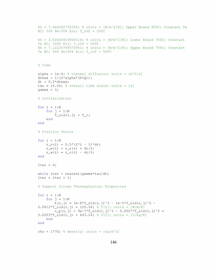
146

%h = 7.666060738358; % units = [W/m^2/K]; Upper Bound 850C; Constant Tw BC; 50% He/50% Air; T_inf = 500C %h = 3.53442419860516; % units = [W/m^2/K]; Lower Bound 750C; Constant Tw BC; 100% Air; T_inf = 500C %h = 7.12226789075961; % units = [W/m^2/K]; Upper Bound 750C; Constant Tw BC; 50% He/50% Air; T_inf = 500C % Time alpha = 1e-4; % thermal diffusion; units = [m^2/s] dtmax = 1/(2*alpha*(P+Q)); dt = 0.2*dtmax; tau = 16.06; % overall time scale; units = [s] gamma = 3; % Initialization for i = 1:N for j = 1:M T_old(i,j) = T_i; end end % Position Vector for i = 1:N r_o(i) = 0.5*(2*i - 1)*dr; r_e(i) = r_o(i) + dr/2; r_w(i) = r_o(i) - dr/2; end iter = 0; while iter < nearest(gamma*tau/dt) iter = iter + 1; % Support Column Thermophysical Properties for i = 1:N for j = 1:M k(i,j) = 3e-8*T_old(i,j)^3 - 1e-5*T_old(i,j)^2 - 0.0612*T_old(i,j) + 125.56; % T[C]; units = [W/m/K] c_p(i,j) = 9e-7*T_old(i,j)^3 - 0.0027*T_old(i,j)^2 + 3.0203*T_old(i,j) + 643.24; % T[C]; units = [J/kg/K] end end rho = 1770; % density; units = [kg/m^3]

147

% Interior Cells for i = 2:N-1 for j = 2:M-1 k_e = (k(i+1,j) + k(i,j))/2; k_w = (k(i-1,j) + k(i,j))/2; k_n = (k(i,j+1) + k(i,j))/2; k_s = (k(i,j-1) + k(i,j))/2; T(i,j) = dt/(rho*c_p(i,j))*(1/(r_o(i)*dr^2)*(k_w*r_w(i)*T_old(i-1,j)-... (k_w*r_w(i)+k_e*r_e(i))*T_old(i,j)+k_e*r_e(i)*T_old(i+1,j))+... 1/dz^2*(k_s*T_old(i,j-1)-(k_s+k_n)*T_old(i,j)+k_n*T_old(i,j+1)))+... T_old(i,j); end end % Top Boundary for i = 2:N-1 j = M; k_e = (k(i+1,j) + k(i,j))/2; k_w = (k(i-1,j) + k(i,j))/2; k_o = k(i,j); k_s = (k(i,j-1) + k(i,j))/2; T(i,j) = dt/(rho*c_p(i,j))*(1/(r_o(i)*dr^2)*(k_w*r_w(i)*T_old(i-1,j)-... (k_w*r_w(i)+k_e*r_e(i))*T_old(i,j)+k_e*r_e(i)*T_old(i+1,j))+... 1/dz^2*((k_o/3+k_s)*T_old(i,j-1)-(3*k_o+k_s)*T_old(i,j)+(8/3)*k_o*T_t))+... T_old(i,j); end % Bottom Boundary for i = 2:N-1 j = 1; k_e = (k(i+1,j) + k(i,j))/2; k_w = (k(i-1,j) + k(i,j))/2; k_n = (k(i,j+1) + k(i,j))/2; k_o = k(i,j); T(i,j) = dt/(rho*c_p(i,j))*(1/(r_o(i)*dr^2)*(k_w*r_w(i)*T_old(i-1,j)-... (k_e*r_e(i)+k_w*r_w(i))*T_old(i,j)+k_e*r_e(i)*T_old(i+1,j))+... 1/dz^2*((8/3)*k_o*T_b-(k_n+3*k_o)*T_old(i,j)+(k_n+k_o/3)*T_old(i,j+1)))+... T_old(i,j); end

148

% Right Boundary for j = 2:M-1 i = N; k_o = k(i,j); k_w = (k(i-1,j) + k(i,j))/2; k_n = (k(i,j+1) + k(i,j))/2; k_s = (k(i,j-1) + k(i,j))/2; T(i,j) = dt/(rho*c_p(i,j))*(1/(r_o(i)*dr)*(-1*h*r_e(i)*... ((3*T_old(i,j)-T_old(i-1,j))/2-T_inf)-k_w*r_w(i)/dr*(T_old(i,j)-T_old(i-1,j)))+... 1/dz^2*(k_s*T_old(i,j-1)-(k_n+k_s)*T_old(i,j)+k_n*T_old(i,j+1)))+T_old(i,j); end % Left Boundary for j = 2:M-1 i = 1; k_e = (k(i+1,j) + k(i,j))/2; k_o = k(i,j); k_n = (k(i,j+1) + k(i,j))/2; k_s = (k(i,j-1) + k(i,j))/2; T(i,j) = dt/(rho*c_p(i,j))*(1/(r_o(i)*dr^2)*(k_e*r_e(i)*T_old(i+1,j)-... k_e*r_e(i)*T_old(i,j))+1/dz^2*(k_s*T_old(i,j-1)-... (k_s+k_n)*T_old(i,j)+k_n*T_old(i,j+1)))+T_old(i,j); end % Top-Right Cell i = N; j = M; k_o = k(i,j); k_w = (k(i-1,j) + k(i,j))/2; k_s = (k(i,j-1) + k(i,j))/2; T(i,j) = dt/(rho*c_p(i,j))*(1/(r_o(i)*dr)*(-1*h*r_e(i)*... ((3*T_old(i,j)-T_old(i-1,j))/2-T_inf)-k_w*r_w(i)/dr*(T_old(i,j)-T_old(i-1,j)))+... (1/dz^2)*((8/3)*k_o*T_t-(3*k_o+k_s)*T_old(i,j)+(k_o/3+k_s)*T_old(i,j-1)))+T_old(i,j); % Bottom-Right Cell i = N; j = 1; k_o = k(i,j); k_w = (k(i-1,j) + k(i,j))/2; k_n = (k(i,j+1) + k(i,j))/2; T(i,j) = dt/(rho*c_p(i,j))*(1/(r_o(i)*dr)*(-1*h*r_e(i)*...

149

((3*T_old(i,j)-T_old(i-1,j))/2-T_inf)-k_w*r_w(i)/dr*(T_old(i,j)-T_old(i-1,j)))+... (1/dz^2)*((8/3)*k_o*T_b-(k_n+3*k_o)*T_old(i,j)+(k_n+k_o/3)*T_old(i,j+1)))+T_old(i,j+1); % Bottom-Left Corner i = 1; j = 1; k_o = k(i,j); k_e = (k(i+1,j) + k(i,j))/2; k_n = (k(i,j+1) + k(i,j))/2; T(i,j) = dt/(rho*c_p(i,j))*(1/(r_o(i)*dr^2)*(k_e*r_e(i)*T_old(i+1,j)-... k_e*r_e(i)*T_old(i,j))+(1/dz^2)*((8/3)*k_o*T_b-(3*k_o+k_n)*T_old(i,j)+... (k_n+k_o/3)*T_old(i,j+1)))+T_old(i,j); % Top-Left Corner i = 1; j = M; k_e = (k(i+1,j) + k(i,j))/2; k_s = (k(i,j-1) + k(i,j))/2; k_o = k(i,j); T(i,j) = dt/(rho*c_p(i,j))*(1/(r_o(i)*dr^2)*(k_e*r_e(i)*T_old(i+1,j)-... k_e*r_e(i)*T_old(i,j))+(1/dz^2)*((8/3)*k_o*T_t-(3*k_o+k_s)*T_old(i,j)+... (k_o/3+k_s)*T_old(i,j-1)))+T_old(i,j); for i = 1:N for j = 1:M T_old(i,j) = T(i,j); end end end contourf(R,Z,T',10)

150

MATLAB code for two-dimensional transient temperature distribution of support column in scaled-down test section

%%% 2-D (Cylindrical Coordinates) Transient Heat Equation for VHTR Support Column %%% Rod (IG-110 Graphite) Using Explicit Time-Marching Method; Finite Volume Discretization; %%% Uniform Mesh; Non-Constant Thermophysical Properties %%% Scaled-down Geometry %%% Dirichlet BCs for top and bottom clc; clear all; close all format long % Geometry Lr = 0.0275; % units = [m] Lz = 0.3556; % units = [m] N = 40; % Number of Cells in Horizontal (r) Direction M = 200; % Number of Cells in Vertical (z) Direction dr = Lr/N; % Cell Width - Horizontal Direction dz = Lz/M; % Cell Height - Vertical Direction P = 1/dr^2; Q = 1/dz^2; R = (dr/2)/Lr:dr/Lr:Lr/Lr; Z = (dz/2)/Lz:dz/Lz:Lz/Lz; % Temperatures T_t = 750; % units = [C]; Upper Boundary Condition T_b = 750; % units = [C]; Lower Boundary Condition T_inf = 25; % units = [C]; Far-field Temperature T_i = 750; % units = [C]; Initial Temperature Condition % Heat Transfer Coefficients %h = 7.9490104123302; % units = [W/m^2/K]; Lower Bound 750C; Constant Tw BC; 100% Air; T_inf = 25C h = 15.5713213816995; % units = [W/m^2/K]; Upper Bound 750C; Constant Tw BC; 100% He; T_inf = 25C %h = 5.52941690843639; %% units = [W/m^2/K]; Lower Bound 750C; Constant Tw BC; 100% Air; T_inf = 500C %h = 10.577265041911; % units = [W/m^2/K]; Upper Bound 750C; Constant Tw BC; 100% He; T_inf = 500C

151

% Time alpha = 1e-4; % thermal diffusion; units = [m^2/s] dtmax = 1/(2*alpha*(P+Q)); dt = 0.2*dtmax; tau = 5.67; % overall time scale; units = [s] gamma = 3; % Initialization for i = 1:N for j = 1:M T_old(i,j) = T_i; end end % Position Vector for i = 1:N r_o(i) = 0.5*(2*i - 1)*dr; r_e(i) = r_o(i) + dr/2; r_w(i) = r_o(i) - dr/2; end iter = 0; while iter < nearest(gamma*tau/dt) iter = iter + 1; % Support Column Thermophysical Properties for i = 1:N for j = 1:M k(i,j) = 3e-8*T_old(i,j)^3 - 1e-5*T_old(i,j)^2 - 0.0612*T_old(i,j) + 125.56; % T[C]; units = [W/m/K] c_p(i,j) = 9e-7*T_old(i,j)^3 - 0.0027*T_old(i,j)^2 + 3.0203*T_old(i,j) + 643.24; % T[C]; units = [J/kg/K] end end rho = 1770; % density; units = [kg/m^3] % Interior Cells for i = 2:N-1 for j = 2:M-1 k_e = (k(i+1,j) + k(i,j))/2; k_w = (k(i-1,j) + k(i,j))/2; k_n = (k(i,j+1) + k(i,j))/2; k_s = (k(i,j-1) + k(i,j))/2;

152

T(i,j) = dt/(rho*c_p(i,j))*(1/(r_o(i)*dr^2)*(k_w*r_w(i)*T_old(i-1,j)-... (k_w*r_w(i)+k_e*r_e(i))*T_old(i,j)+k_e*r_e(i)*T_old(i+1,j))+... 1/dz^2*(k_s*T_old(i,j-1)-(k_s+k_n)*T_old(i,j)+k_n*T_old(i,j+1)))+... T_old(i,j); end end % Top Boundary for i = 2:N-1 j = M; k_e = (k(i+1,j) + k(i,j))/2; k_w = (k(i-1,j) + k(i,j))/2; k_o = k(i,j); k_s = (k(i,j-1) + k(i,j))/2; T(i,j) = dt/(rho*c_p(i,j))*(1/(r_o(i)*dr^2)*(k_w*r_w(i)*T_old(i-1,j)-... (k_w*r_w(i)+k_e*r_e(i))*T_old(i,j)+k_e*r_e(i)*T_old(i+1,j))+... 1/dz^2*((k_o/3+k_s)*T_old(i,j-1)-(3*k_o+k_s)*T_old(i,j)+(8/3)*k_o*T_t))+... T_old(i,j); end % Bottom Boundary for i = 2:N-1 j = 1; k_e = (k(i+1,j) + k(i,j))/2; k_w = (k(i-1,j) + k(i,j))/2; k_n = (k(i,j+1) + k(i,j))/2; k_o = k(i,j); T(i,j) = dt/(rho*c_p(i,j))*(1/(r_o(i)*dr^2)*(k_w*r_w(i)*T_old(i-1,j)-... (k_e*r_e(i)+k_w*r_w(i))*T_old(i,j)+k_e*r_e(i)*T_old(i+1,j))+... 1/dz^2*((8/3)*k_o*T_b-(k_n+3*k_o)*T_old(i,j)+(k_n+k_o/3)*T_old(i,j+1)))+... T_old(i,j); end % Right Boundary for j = 2:M-1 i = N; k_o = k(i,j); k_w = (k(i-1,j) + k(i,j))/2; k_n = (k(i,j+1) + k(i,j))/2; k_s = (k(i,j-1) + k(i,j))/2;

153

T(i,j) = dt/(rho*c_p(i,j))*(1/(r_o(i)*dr)*(-1*h*r_e(i)*... ((3*T_old(i,j)-T_old(i-1,j))/2-T_inf)-k_w*r_w(i)/dr*(T_old(i,j)-T_old(i-1,j)))+... 1/dz^2*(k_s*T_old(i,j-1)-(k_n+k_s)*T_old(i,j)+k_n*T_old(i,j+1)))+T_old(i,j); end % Left Boundary for j = 2:M-1 i = 1; k_e = (k(i+1,j) + k(i,j))/2; k_o = k(i,j); k_n = (k(i,j+1) + k(i,j))/2; k_s = (k(i,j-1) + k(i,j))/2; T(i,j) = dt/(rho*c_p(i,j))*(1/(r_o(i)*dr^2)*(k_e*r_e(i)*T_old(i+1,j)-... k_e*r_e(i)*T_old(i,j))+1/dz^2*(k_s*T_old(i,j-1)-... (k_s+k_n)*T_old(i,j)+k_n*T_old(i,j+1)))+T_old(i,j); end % Top-Right Cell i = N; j = M; k_o = k(i,j); k_w = (k(i-1,j) + k(i,j))/2; k_s = (k(i,j-1) + k(i,j))/2; T(i,j) = dt/(rho*c_p(i,j))*(1/(r_o(i)*dr)*(-1*h*r_e(i)*... ((3*T_old(i,j)-T_old(i-1,j))/2-T_inf)-k_w*r_w(i)/dr*(T_old(i,j)-T_old(i-1,j)))+... (1/dz^2)*((8/3)*k_o*T_t-(3*k_o+k_s)*T_old(i,j)+(k_o/3+k_s)*T_old(i,j-1)))+T_old(i,j); % Bottom-Right Cell i = N; j = 1; k_o = k(i,j); k_w = (k(i-1,j) + k(i,j))/2; k_n = (k(i,j+1) + k(i,j))/2; T(i,j) = dt/(rho*c_p(i,j))*(1/(r_o(i)*dr)*(-1*h*r_e(i)*... ((3*T_old(i,j)-T_old(i-1,j))/2-T_inf)-k_w*r_w(i)/dr*(T_old(i,j)-T_old(i-1,j)))+... (1/dz^2)*((8/3)*k_o*T_b-(k_n+3*k_o)*T_old(i,j)+(k_n+k_o/3)*T_old(i,j+1)))+T_old(i,j+1); % Bottom-Left Corner i = 1; j = 1;

154

k_o = k(i,j); k_e = (k(i+1,j) + k(i,j))/2; k_n = (k(i,j+1) + k(i,j))/2; T(i,j) = dt/(rho*c_p(i,j))*(1/(r_o(i)*dr^2)*(k_e*r_e(i)*T_old(i+1,j)-... k_e*r_e(i)*T_old(i,j))+(1/dz^2)*((8/3)*k_o*T_b-(3*k_o+k_n)*T_old(i,j)+... (k_n+k_o/3)*T_old(i,j+1)))+T_old(i,j); % Top-Left Corner i = 1; j = M; k_e = (k(i+1,j) + k(i,j))/2; k_s = (k(i,j-1) + k(i,j))/2; k_o = k(i,j); T(i,j) = dt/(rho*c_p(i,j))*(1/(r_o(i)*dr^2)*(k_e*r_e(i)*T_old(i+1,j)-... k_e*r_e(i)*T_old(i,j))+(1/dz^2)*((8/3)*k_o*T_t-(3*k_o+k_s)*T_old(i,j)+... (k_o/3+k_s)*T_old(i,j-1)))+T_old(i,j); for i = 1:N for j = 1:M T_old(i,j) = T(i,j); end end end contourf(R,Z,T',10)

155

MATLAB code for two-dimensional transient temperature distribution of shell/heater system in scaled-down test section

%%% 2-D Transient Heat Equation for VHTR/Scaled-down Model Heater/Support Column %%% Rod (IG-110 Graphite) Using Explicit Time-Marching Method; Finite Volume %%%Discretization; Uniform Mesh; Non-Constant Thermophysical Properties %%% Dirichlet BCs for top and bottom clc; clear all; close all % Rod Shell Geometry Lr = 0.0148; % units = [m] Lz = 14*0.0254; % units = [m] N = 20; % Number of Cells in Horizontal (x) Direction M = 200; % Number of Cells in Vertical (y) Direction dr = Lr/N; % Cell Width - Horizontal Direction dz = Lz/M; % Cell Height - Vertical Direction P = 1/dr^2; Q = 1/dz^2; R = (0.0127+dr/2)/0.0275:dr/0.0275:0.0275/0.0275; Z = (dz/2)/Lz:dz/Lz:Lz/Lz; % Heater Geometry and Output Q_dot = 125; % units = [W] D = 0.935*2.54/100; % heater diameter; units = [m] H = 14*2.54/100; % heater length; units = [m] A_s = pi*D*H; % heater surface area; units = [m^2] q1 = Q_dot/A_s; % heater heat flux; units = [W/m^2] A2 = pi*0.0254*Lz; q = q1*A_s/A2; % Temperatures T_t = 750; % units = [C] T_b = 750; % units = [C] T_inf = 25; % units = [C] T_i = 750; % units = [C] % Heat Transfer Coefficients %h = 7.9490104123302; % units = [W/m^2/K]; Lower Bound 750C; Constant Tw BC; 100% Air; T_inf = 25C

156

h = 15.5713213816995; % units = [W/m^2/K]; Upper Bound 750C; Constant Tw BC; 100% He; T_inf = 25C %h = 5.52941690843639; %% units = [W/m^2/K]; Lower Bound 750C; Constant Tw BC; 100% Air; T_inf = 500C %h = 10.577265041911; % units = [W/m^2/K]; Upper Bound 750C; Constant Tw BC; 100% He; T_inf = 500C % Time alpha = 1e-4; % thermal diffusion; units = [m^2/s] dtmax = 1/(2*alpha*(P+Q)); dt = 0.2*dtmax; tau = 5.67; % overall time scale; units = [s] gamma = 3; % Initialization for i = 1:N for j = 1:M T_old(i,j) = T_i; end end % Position Vector for i = 1:N r_o(i) = 0.5*(2*i - 1)*dr + 0.0127; r_e(i) = r_o(i) + dr/2; r_w(i) = r_o(i) - dr/2; end iter = 0; while iter < nearest(gamma*tau/dt) iter = iter + 1; % Support Column Thermophysical Properties for i = 1:N for j = 1:M k(i,j) = 3e-8*T_old(i,j)^3 - 1e-5*T_old(i,j)^2 - 0.0612*T_old(i,j) + 125.56; % T[C]; units = [W/m/K] c_p(i,j) = 9e-7*T_old(i,j)^3 - 0.0027*T_old(i,j)^2 + 3.0203*T_old(i,j) + 643.24; % T[C]; units = [J/kg/K] end end rho = 1770; % density; units = [kg/m^3] % Interior Cells

157

for i = 2:N-1 for j = 2:M-1 k_e = (k(i+1,j) + k(i,j))/2; k_w = (k(i-1,j) + k(i,j))/2; k_n = (k(i,j+1) + k(i,j))/2; k_s = (k(i,j-1) + k(i,j))/2; T(i,j) = dt/(rho*c_p(i,j))*(1/(r_o(i)*dr^2)*(k_w*r_w(i)*T_old(i-1,j)-... (k_w*r_w(i)+k_e*r_e(i))*T_old(i,j)+k_e*r_e(i)*T_old(i+1,j))+... 1/dz^2*(k_s*T_old(i,j-1)-(k_s+k_n)*T_old(i,j)+k_n*T_old(i,j+1)))+... T_old(i,j); end end % Top Boundary for i = 2:N-1 j = M; k_e = (k(i+1,j) + k(i,j))/2; k_w = (k(i-1,j) + k(i,j))/2; k_o = k(i,j); k_s = (k(i,j-1) + k(i,j))/2; T(i,j) = dt/(rho*c_p(i,j))*(1/(r_o(i)*dr^2)*(k_w*r_w(i)*T_old(i-1,j)-... (k_w*r_w(i)+k_e*r_e(i))*T_old(i,j)+k_e*r_e(i)*T_old(i+1,j))+... 1/dz^2*((k_o/3+k_s)*T_old(i,j-1)-(3*k_o+k_s)*T_old(i,j)+(8/3)*k_o*T_t))+... T_old(i,j); end % Bottom Boundary for i = 2:N-1 j = 1; k_e = (k(i+1,j) + k(i,j))/2; k_w = (k(i-1,j) + k(i,j))/2; k_n = (k(i,j+1) + k(i,j))/2; k_o = k(i,j); T(i,j) = dt/(rho*c_p(i,j))*(1/(r_o(i)*dr^2)*(k_w*r_w(i)*T_old(i-1,j)-... (k_e*r_e(i)+k_w*r_w(i))*T_old(i,j)+k_e*r_e(i)*T_old(i+1,j))+... 1/dz^2*((8/3)*k_o*T_b-(k_n+3*k_o)*T_old(i,j)+(k_n+k_o/3)*T_old(i,j+1)))+... T_old(i,j); end

158

% Right Boundary for j = 2:M-1 i = N; k_o = k(i,j); k_w = (k(i-1,j) + k(i,j))/2; k_n = (k(i,j+1) + k(i,j))/2; k_s = (k(i,j-1) + k(i,j))/2; T(i,j) = dt/(rho*c_p(i,j))*(1/(r_o(i)*dr)*(-1*h*r_e(i)*... ((3*T_old(i,j)-T_old(i-1,j))/2-T_inf)-k_w*r_w(i)/dr*(T_old(i,j)-T_old(i-1,j)))+... 1/dz^2*(k_s*T_old(i,j-1)-(k_n+k_s)*T_old(i,j)+k_n*T_old(i,j+1)))+T_old(i,j); end % Left Boundary for j = 2:M-1 i = 1; k_e = (k(i+1,j) + k(i,j))/2; k_o = k(i,j); k_n = (k(i,j+1) + k(i,j))/2; k_s = (k(i,j-1) + k(i,j))/2; T(i,j) = dt/(rho*c_p(i,j))*(1/(r_o(i)*dr)*(k_e*r_e(i)/dr*(T_old(i+1,j)-T_old(i,j))+... q*r_w(i))+1/dz^2*(k_s*T_old(i,j-1)-(k_s+k_n)*T_old(i,j)+k_n*T_old(i,j+1)))+... T_old(i,j); end % Top-Right Cell i = N; j = M; k_o = k(i,j); k_w = (k(i-1,j) + k(i,j))/2; k_s = (k(i,j-1) + k(i,j))/2; T(i,j) = dt/(rho*c_p(i,j))*(1/(r_o(i)*dr)*(-1*h*r_e(i)*... ((3*T_old(i,j)-T_old(i-1,j))/2-T_inf)-k_w*r_w(i)/dr*(T_old(i,j)-T_old(i-1,j)))+... (1/dz^2)*((8/3)*k_o*T_t-(3*k_o+k_s)*T_old(i,j)+(k_o/3+k_s)*T_old(i,j-1)))+T_old(i,j); % Bottom-Right Cell i = N; j = 1; k_o = k(i,j); k_w = (k(i-1,j) + k(i,j))/2; k_n = (k(i,j+1) + k(i,j))/2; T(i,j) = dt/(rho*c_p(i,j))*(1/(r_o(i)*dr)*(-1*h*r_e(i)*...

159

((3*T_old(i,j)-T_old(i-1,j))/2-T_inf)-k_w*r_w(i)/dr*(T_old(i,j)-T_old(i-1,j)))+... (1/dz^2)*((8/3)*k_o*T_b-(k_n+3*k_o)*T_old(i,j)+(k_n+k_o/3)*T_old(i,j+1)))+T_old(i,j+1); % Bottom-Left Corner i = 1; j = 1; k_o = k(i,j); k_e = (k(i+1,j) + k(i,j))/2; k_n = (k(i,j+1) + k(i,j))/2; T(i,j) = dt/(rho*c_p(i,j))*(1/(r_o(i)*dr)*(k_e*r_e(i)/dr*T_old(i+1,j)-... k_e*r_e(i)/dr*T_old(i,j)+q*r_w(i))+(1/dz^2)*((8/3)*k_o*T_b-(3*k_o+k_n)*T_old(i,j)+... (k_n+k_o/3)*T_old(i,j+1)))+T_old(i,j); % Top-Left Corner i = 1; j = M; k_e = (k(i+1,j) + k(i,j))/2; k_s = (k(i,j-1) + k(i,j))/2; k_o = k(i,j); T(i,j) = dt/(rho*c_p(i,j))*(1/(r_o(i)*dr)*(k_e*r_e(i)/dr*T_old(i+1,j)-... k_e*r_e(i)/dr*T_old(i,j)+q*r_w(i))+(1/dz^2)*((8/3)*k_o*T_t-(3*k_o+k_s)*T_old(i,j)+... (k_o/3+k_s)*T_old(i,j-1)))+T_old(i,j); for i = 1:N for j = 1:M T_old(i,j) = T(i,j); end end end contourf(R,Z,T',10)

160

MATLAB code for mixed mean temperature in reactor/containment system without air mass reduction

%%% Mixed Mean Temperature After Depressurization clc; clear all; close all %%% Initial Conditions and Parameters Ph = 7e6; %% Absolute Pressure of Vessel; units = [Pa] Vh = 265.9; %% Volume of Pressure Vessel; units = [m^3] Th = 1123; %% Helium Temperature inside Vessel; units = [K] Pa = 101325; %% Absolute Pressure of Containment; units = [Pa] Va = 25000; %% Volume of Containment; units = [m^3] Ta = 298; %% Air Temperature in Containment; units = [K] %%% Constants and Thermo-physical properties R = 8.314462175; %% Universal Gas Constant; units = [J/mol/K] Mh = 0.004002602; %% Molar mass of helium; units = [kg/mol] Ma = 0.0289656; %% Molar mass of air; units = [kg/mol] nh = Ph*Vh/(R*Th); %% number of helium moles; units = [mol] nai = Pa*Va/(R*Ta); %% numbrt of air moles; units = [mol] mh = Mh*nh; %% mass of helium in the system; units = [kg] mai = Ma*nai; %% initial mass of air in the system; units = [kg] chi = 3116; %% specific heat capacity for helium; units = [J/kg/K] cni = (1000/0.239005736/28)*(1/1.4)*(9.3355-122.56*(Ta/100)^-1.5+... 256.38*(Ta/100)^-2 - 196.08*(Ta/100)^-3); %% specific heat for nitrogen; units = [J/kg/K] coi = (1000/0.239005736/32)*(1/1.4)*(8.9425 + 4.8044e-3*(Ta/100)^1.5 -... 42.679*(Ta/100)^-1.5 + 56.615*(Ta/100)^-2); %% specific heat for oxygen; units = [J/kg/K] cai = 0.8*cni + 0.2*coi; %% specific heat for air; units = [J/kg/K] iter = 0; tol = 1e-6; Pf = (Ph + Pa)/2; Tf = (Th + Ta)/2; Pf_new = 0; while abs(Pf_new - Pf) > tol Pf = Pf_new; cnf = (1000/0.239005736/28)*(1/1.4)*(9.3355-122.56*(Tf/100)^-1.5+...

161

256.38*(Tf/100)^-2 - 196.08*(Tf/100)^-3); cof = (1000/0.239005736/32)*(1/1.4)*(8.9425 + 4.8044e-3*(Tf/100)^1.5 -... 42.679*(Tf/100)^-1.5 + 56.615*(Tf/100)^-2); caf = 0.8*cnf + 0.2*cof; chf = 3116; Tf = (mh*chi*Th + mai*cai*Ta)/(mh*chf + mai*caf); Pf_new = (nh+nai)*R*Tf/(Va+Vh); iter = iter +1; end

162

MATLAB code for mixed mean temperature in reactor/containment system with air mass reduction

%%% Mixed Mean Temperature and Air-to-Helium Mole Ratio After Depressurization clc; clear all; close all %%% Initial Conditions and Parameters % Scaled-down Parameters for Vessel %Ph = 75*6894.759; %% Absolute Pressure of Pressure Vessel; units = [Pa] %Vh = 0.209835; %% Volume of Pressure Vessel; units = [m^3] %Th = 1023; %% Helium Temperature inside Vessel; units = [K] % Prototypic Parameters for Vessel Th = 1123; %% Helium Temperature inside Vessel; units = [K] Ph = 7e6; %% Absolute Pressure of Vessel; units = [Pa] Vh = 265.9; %% Volume of Pressure Vessel; units = [m^3] % Scaled-down Parameters for Containment %Pa = 101325; %% Absolute Pressure of Containment; units = [Pa] %Va = 1; %% Free Volume of Containment; units = [m^3] %Ta = 298; %% Air Temperature in Containment; units = [K] % Prototypic Parameters for Containment Pa = 101325; %% Absolute Pressure of Containment; units = [Pa] Va = 25000; %% Volume of Containment; units = [m^3] Ta = 298; %% Air Temperature in Containment; units = [K] %%% Constants and Thermo-physical properties R = 8.314462175; %% Universal Gas Constant; units = [J/mol/K] Mh = 0.004002602; %% Molar mass of helium; units = [kg/mol] nhi = Ph*Vh/(R*Th); %% number of helium moles; units = [mol] nhf = nhi; mhi = Mh*nhi; %% mass of helium in the system; units = [kg] mhf = Mh*nhi; %% mass of helium in the system; units = [kg] chi = 3116; %% specific heat capacity for helium; units = [J/kg/K]

163

Ma = 0.0289656; %% Molar mass of air; units = [kg/mol] nai = Pa*Va/(R*Ta); %% numbrt of air moles; units = [mol] naf = nai; mai = Ma*nai; %% initial mass of air in the system; units = [kg] maf = Ma*naf; %% initial mass of air in the system; units = [kg] cni = (1000/0.239005736/28)*(1/1.4)*(9.3355-122.56*(Ta/100)^-1.5+... 256.38*(Ta/100)^-2 - 196.08*(Ta/100)^-3); %% specific heat for nitrogen; units = [J/kg/K] coi = (1000/0.239005736/32)*(1/1.4)*(8.9425 + 4.8044e-3*(Ta/100)^1.5 -... 42.679*(Ta/100)^-1.5 + 56.615*(Ta/100)^-2); %% specific heat for oxygen; units = [J/kg/K] cai = 0.8*cni + 0.2*coi; %% specific heat for air; units = [J/kg/K] %%% Parameters for Outflow T_esc = Ta; cpn = (1000/0.239005736/28)*(9.3355-122.56*(T_esc/100)^-1.5+... 256.38*(T_esc/100)^-2 - 196.08*(T_esc/100)^-3); cpo = (1000/0.239005736/32)*(8.9425 + 4.8044e-3*(T_esc/100)^1.5 -... 42.679*(T_esc/100)^-1.5 + 56.615*(T_esc/100)^-2); cp_esc = 0.8*cpn + 0.2*cpo; %%% Iterative Loop iter = 0; tol = 1e-8; Pf = (Ph + Pa)/2; Tf = (Th + Ta)/2; ma_esc = mai - maf; while abs(Pf - Pa) > tol cnf = (1000/0.239005736/28)*(1/1.4)*(9.3355-122.56*(Tf/100)^-1.5+... 256.38*(Tf/100)^-2 - 196.08*(Tf/100)^-3); cof = (1000/0.239005736/32)*(1/1.4)*(8.9425 + 4.8044e-3*(Tf/100)^1.5 -... 42.679*(Tf/100)^-1.5 + 56.615*(Tf/100)^-2); caf = 0.8*cnf + 0.2*cof; chf = 3116; Tf = (-1*ma_esc*cp_esc*T_esc + mhi*chi*Th + mai*cai*Ta)/(mhf*chf + maf*caf); Pf_new = (nhf+naf)*R*Tf/(Va+Vh); if abs(Pf_new - Pa) > tol naf = Pa*(Va+Vh)/(R*Tf) - nhf; maf = naf*Ma; ma_esc = mai - maf; end

164

Pf = Pf_new; iter = iter + 1; end Tf naf/nhf ma_esc/mai*100

165

MATLAB code for blowdown transient analysis of prototypic GT-MHR

%%% Blowdown Transient Analysis for Prototypic GT-MHR clc; clear all; close all % Givens R = 2076.9; % helium gas constant; units = [J/kg/K] c_p = 5190.1; % specific heat capacity under constant pressure for helium; units = [J/kg/K] c_v = 3122; % specific heat capacity under constant volume for helium; units = [J/kg/K] c_w = 1071.71; % specific heat capacity for vessel and internals; units = [J/kg/K] V_w = 799.05; % volume of vessel structure and internals; units = [m^3] rho_w = 4307.79; % density of vessel structure and internals; units = [kg/m^3] As = 10432; % total surface area; units = [m^2] V = 265.9; % vessel free volume; units = [m^3] Po = 6e8; % steady-state reactor power; units = [W] gamma = 5/3; % ratio of specific heats for helium; unitless T_amb = 365; % ambient temperature (confinement temperature); units = [K] rho_amb = 0.13359; % ambient helium density; units = [kg/m^3] mu_amb = 2.2804e-5; % ambient helium viscosity; units = [kg/m/s] or [Pa*s] a = sqrt(gamma*R*T_amb); % speed of sound at exit of pipe; units = [m/s] p_amb = 101325; % ambient pressure; units = [Pa] mu_i = 5.0180e-5; % initial helium viscosity; units = [Pa*s] rho_i = 2.9796; % intial helium density; units = [kg/m^3] p_i = 7000000; % initial vessel pressure; units = [Pa] m_i = rho_i*V; % initial helium mass in vessel; units = [kg] Ti = 1123.15; % initial helium temperature; units = [K] To = 273.15; % abs. temperature; units = [K] Twi = 1123.15; % initial wall temperature; units = [K] h = 2; % heat transfer coefficient; units = [W/m^2/K] eps = 4.5e-5; % pipe equivalent roughness for a new commercial steel pipe % units = [m] L = 2.86; % length of pipe; units = [m] d1 = 1.4238; % inner diameter of hot duct; units = [m] d2 = 1.5; % outer diameter of hot duct; units = [m] d3 = 2.29; % inner diameter of cold duct; units = [m]

166

Ac = pi/4*(d3^2 - d2^2 + d1^2); % flow area of duct; units = [m^2] Pw = pi*(d3 + d2 + d1); % wetted perimeter of duct; units = [m] D = 4*Ac/Pw; % hydraulic diameter; units = [m] K_c = 0.5; % Loss coefficient for a sudden contraction; unitless f_g = .002; % friction factor guess; unitless alpha2 = 1; % kinetic energy coefficients; unitless tol = 1e-6; % tolerance t_max = 60; % duration of blowdown transient; units = [s] delta_t = .001; % temporal step; units = [s] n = floor(t_max/delta_t); % number of time steps; unitless err = 1; err1 = 1; T(1) = Ti; Tw(1) = Twi; p(1) = p_i; m(1) = m_i; rho(1) = rho_i; mu(1) = mu_i; for i = 1:n % i = 1; t(i) = (i-1)*delta_t; rho_avg(i) = (rho(i) + rho_amb)/2; mu_avg(i) = (mu(i) + mu_amb)/2; while abs(err) >= tol v_g(i) = sqrt((p(i)-p_amb)/(rho_avg(i)*(alpha2/2 + 1/2*(K_c + f_g*L/D)))); if v_g(i) >= a Re_g(i) = rho_avg(i)*a*D/mu_avg(i); else Re_g(i) = rho_avg(i)*v_g(i)*D/mu_avg(i); end if Re_g(i) >= 4000 f1(i) = 0.184*Re_g(i)^-0.2; while abs(err1) >= tol f(i) = (1/(-2*log10((eps/D)/3.7 + 2.51/(Re_g(i)*sqrt(f1(i))))))^2; % Colbrook Equation err1 = f1(i) - f(i); f1(i) = f(i); end else f(i) = 64/Re_g(i); end v(i) = sqrt((p(i)-p_amb)/(rho_avg(i)*(alpha2/2 + 1/2*(K_c + f(i)*L/D)))); err = v_g(i) - v(i); f_g = f(i); end if v(i) >= a

167

m_dot(i) = rho_avg(i)*Ac*a; Re(i) = rho_avg(i)*a*D/mu_avg(i); else m_dot(i) = rho_avg(i)*Ac*v(i); Re(i) = rho_avg(i)*v(i)*D/mu_avg(i); end T(i+1) = delta_t*h*As/(c_v*m(i))*Tw(i) + (1 - delta_t*(h*As + m_dot(i)*R)... /(c_v*m(i)))*T(i); Tw(i+1) = delta_t*0.066*Po*((i-1)*delta_t + (delta_t)^2)^-0.2/(rho_w*V_w*c_w)... + delta_t*h*As/(rho_w*V_w*c_w)*T(i) + (1 - delta_t*h*As/(rho_w*V_w*c_w))*Tw(i); t(i+1) = t(i) + delta_t; m(i+1) = m(i) - m_dot(i)*delta_t; mu(i+1) = 1.865e-5*(T(i+1)/To)^0.7; rho(i+1) = rho(i) - m_dot(i)*delta_t/V; p(i+1) = rho(i+1)*R*T(i+1); if p(i+1) <= p_amb break end err = err + 1; err1 = err1 + 1; end plot(t,p) grid on xlabel('Time (s)'); ylabel('Pressure (Pa)'); title('Prototype Geometry - Pressure v. Time'); figure plot(t,T) grid on xlabel('Time (s)'); ylabel('Helium Temperature (K)'); title('Prototype Geometry - Helium Temperature v. Time'); figure plot(t,Tw) grid on xlabel('Time (s)'); ylabel('Solid Temperature (K)'); title('Prototype Geometry - Solid Temperature v. Time');

168

MATLAB code for blowdown transient analysis of scaled-down test section

%%% Blowdown Transient Analysis for Scaled-down Test Section clc; clear all; close all % Givens R = 2076.9; % helium gas constant; units = [J/kg/K] c_p = 5190.1; % specific heat capacity under constant pressure for helium; units = [J/kg/K] c_v = 3122; % specific heat capacity under constant volume for helium; units = [J/kg/K] c_w = 1071.71; % specific heat capacity for vessel and internals; units = [J/kg/K] V_w = 1.56; % volume of vessel structure and internals; units = [m^3] rho_w = 4307.79; % density of vessel structure and internals; units = [kg/m^3] As = 5.316822; % total surface area; units = [m^2] V = 0.160848; % vessel free volume; units = [m^3] Po = 6*125; % steady-state reactor power; units = [W] gamma = 5/3; % ratio of specific heats for helium; unitless T_amb = 365; % ambient temperature (confinement temperature); units = [K] rho_amb = 0.13359; % ambient helium density; units = [kg/m^3] mu_amb = 2.2804e-5; % ambient helium viscosity; units = [kg/m/s] or [Pa*s] a = sqrt(gamma*R*T_amb); % speed of sound at exit of pipe; units = [m/s] p_amb = 101325; % ambient pressure; units = [Pa] mu_i = 4.6918e-5; % initial helium viscosity; units = [Pa*s] rho_i = 0.24317; % intial helium density; units = [kg/m^3] p_i = 517106; % initial vessel pressure; units = [Pa] m_i = rho_i*V; % initial helium mass in vessel; units = [kg] Ti = 1023.15; % initial helium temperature; units = [K] To = 273.15; % abs. temperature; units = [K] Twi = 1023.15; % initial wall temperature; units = [K] h = 2; % heat transfer coefficient; units = [W/m^2/K] eps = 4.5e-5; % pipe equivalent roughness for a new commercial steel pipe % units = [m] L = 8*.025; % length of pipe; units = [m] d1 = 7.5*0.025; % inner diameter of hot duct; units = [m] Ac = pi/4*d1^2; % flow area of duct; units = [m^2] Pw = pi*d1; % wetted perimeter of duct; units = [m]

169

D = 4*Ac/Pw; % hydraulic diameter; units = [m] K_c = 0.5; % Loss coefficient for a sudden contraction; unitless f_g = .002; % friction factor guess; unitless alpha2 = 1; % kinetic energy coefficients; unitless tol = 1e-6; % tolerance t_max = 60; % duration of blowdown transient; units = [s] delta_t = .00001; % temporal step; units = [s] n = floor(t_max/delta_t); % number of time steps; unitless err = 1; err1 = 1; T(1) = Ti; Tw(1) = Twi; p(1) = p_i; m(1) = m_i; rho(1) = rho_i; mu(1) = mu_i; for i = 1:n % i = 1; t(i) = (i-1)*delta_t; rho_avg(i) = (rho(i) + rho_amb)/2; mu_avg(i) = (mu(i) + mu_amb)/2; while abs(err) >= tol v_g(i) = sqrt((p(i)-p_amb)/(rho_avg(i)*(alpha2/2 + 1/2*(K_c + f_g*L/D)))); if v_g(i) >= a Re_g(i) = rho_avg(i)*a*D/mu_avg(i); else Re_g(i) = rho_avg(i)*v_g(i)*D/mu_avg(i); end if Re_g(i) >= 4000 f1(i) = 0.184*Re_g(i)^-0.2; while abs(err1) >= tol f(i) = (1/(-2*log10((eps/D)/3.7 + 2.51/(Re_g(i)*sqrt(f1(i))))))^2; % Colbrook Equation err1 = f1(i) - f(i); f1(i) = f(i); end else f(i) = 64/Re_g(i); end v(i) = sqrt((p(i)-p_amb)/(rho_avg(i)*(alpha2/2 + 1/2*(K_c + f(i)*L/D)))); err = v_g(i) - v(i); f_g = f(i); end if v(i) >= a m_dot(i) = rho_avg(i)*Ac*a; Re(i) = rho_avg(i)*a*D/mu_avg(i);

170

else m_dot(i) = rho_avg(i)*Ac*v(i); Re(i) = rho_avg(i)*v(i)*D/mu_avg(i); end T(i+1) = delta_t*h*As/(c_v*m(i))*Tw(i) + (1 - delta_t*(h*As + m_dot(i)*R)... /(c_v*m(i)))*T(i); Tw(i+1) = delta_t*0.066*Po*((i-1)*delta_t + (delta_t)^2)^-0.2/(rho_w*V_w*c_w)... + delta_t*h*As/(rho_w*V_w*c_w)*T(i) + (1 - delta_t*h*As/(rho_w*V_w*c_w))*Tw(i); t(i+1) = t(i) + delta_t; m(i+1) = m(i) - m_dot(i)*delta_t; mu(i+1) = 1.865e-5*(T(i+1)/To)^0.7; rho(i+1) = rho(i) - m_dot(i)*delta_t/V; p(i+1) = rho(i+1)*R*T(i+1); if p(i+1) <= p_amb break end err = err + 1; err1 = err1 + 1; end plot(t,p) grid on xlabel('Time (s)'); ylabel('Pressure (Pa)'); title('Scaled-down Test Section - Pressure v. Time'); figure plot(t,T) grid on xlabel('Time (s)'); ylabel('Helium Temperature (K)'); title('Scaled-down Test Section - Helium Temperature v. Time'); figure plot(t,Tw) grid on xlabel('Time (s)'); ylabel('Solid Temperature (K)'); title('Scaled-down Test Section - Solid Temperature v. Time');