Tuning and plateaux for the entropy of $\alpha$-continued fractions

$Page 1: Tuning and plateaux for the entropy of $\alpha$-continued fractions$
TUNING AND PLATEAUX FOR THE ENTROPY OF

α-CONTINUED FRACTIONS

CARLO CARMINATI, GIULIO TIOZZO

Abstract. The entropy h(Tα) of α-continued fraction transformations is knownto be locally monotone outside a closed, totally disconnected set E. We will

exploit the explicit description of the fractal structure of E to investigate the

self-similarities displayed by the graph of the function α 7→ h(Tα). Finally, wecompletely characterize the plateaux occurring in this graph, and classify the

local monotonic behaviour.

1. Introduction

It is a well-known fact that the continued fraction expansion of a real number canbe analyzed in terms of the dynamics of the interval map G(x) :=

{1x

}, known as

the Gauss map. A generalization of this map is given by the family of α-continuedfraction transformations Tα, which will be the object of study of the present paper.For each α ∈ [0, 1], the map Tα : [α− 1, α]→ [α− 1, α] is defined as Tα(0) = 0 and,for x 6= 0,

Tα(x) :=1

|x|− cα,x

where cα,x =⌊

1|x| + 1− α

⌋is a positive integer. Each of these maps is associated to

a different continued fraction expansion algorithm, and the family Tα interpolatesbetween maps associated to well-known expansions: T1 = G is the usual Gaussmap which generates regular continued fractions, while T1/2 is associated to thecontinued fraction to the nearest integer, and T0 generates the by-excess continuedfraction expansion. For more about α-continued fraction expansions, their metricproperties and their relations with other continued fraction expansions we refer to[Na], [Sc], [IK]. This family has also been studied in relation to the Brjuno function[MMY], [MCM].

Every Tα has infinitely many branches, and, for α > 0, all branches are expansiveand Tα admits an invariant probability measure absolutely continuous with respectto Lebesgue measure. Hence, each Tα has a well-defined metric entropy h(α): themetric entropy of the map Tα is proportional to the speed of convergence of thecorresponding expansion algorithm (known as α-euclidean algorithm) [BDV], andto the exponential growth rate of the partial quotients in the α-expansion of typicalvalues [NN].

Nakada [Na], who first investigated the properties of this family of continuedfraction algorithms, gave an explicit formula for h(α) for 1

2 ≤ α ≤ 1, from which itis evident that entropy displays a phase transition phenomenon when the parameter

equals the golden mean g :=√5−12 (see also Figure 1, left):

(1) h(α) =

π2

6 log(1+α) for√5−12 < α ≤ 1

π2

6 log√

5+12

for 12 ≤ α ≤

√5−12

Several authors have studied the behaviour of the metric entropy of Tα as a func-tion of the parameter α ([Ca], [LM], [NN], [KSS]); in particular Luzzi and Marmi

1

arX

iv:1

111.

2554

v2 [

mat

h.D

S] 3

1 M

ay 2

012

2 CARLO CARMINATI, GIULIO TIOZZO

[LM] first produced numerical evidence that the entropy is continuous, althoughit displays many more (even if less evident) phase transition points and it is notmonotone on the interval [0, 1/2]. Subsequently, Nakada and Natsui [NN] identi-fied a dynamical condition that forces the entropy to be, at least locally, monotone:indeed, they noted that for some parameters α, the orbits under Tα of α and α− 1collide after a number of steps, i.e. there exist N,M such that:

(2) TN+1α (α) = TM+1

α (α− 1)

and they proved that, whenever the matching condition (2) holds, h(α) is monotoneon a neighbourhood of α. They also showed that h has mixed monotonic behaviournear the origin: namely, for every δ > 0, in the interval (0, δ) there are intervals onwhich h(α) is monotone, others on which h(α) is increasing and others on whichh(α) is decreasing.

In [CT] it is proven that the set of parameters for which (2) holds actually hasfull measure in parameter space. Moreover, such a set is the union of countablymany open intervals, called maximal quadratic intervals. Each maximal quadraticinterval Ir is labeled by a rational number r and can be thought of as a stabilitydomain in parameter space: indeed, the number of steps M,N it takes for the orbitsto collide is the same for each α ∈ Ir, and even the symbolic orbit of α and α − 1up to the collision is fixed (compare to mode-locking phenomena in the theory ofcircle maps). For this reason, the complement of the union of all Ir is called thebifurcation set or exceptional set E .

Numerical experiments [LM], [CMPT] show the entropy function h(α) displaysself-similar features: the main goal of this paper is to prove such self-similar struc-ture by exploiting the self-similarity of the bifurcation set E .

The way to study the self-similar structure was suggested to us by the unex-pected isomorphism between E and the real slice of the boundary of the Mandel-brot set [BCIT]. In the family of quadratic polynomials, Douady and Hubbard[DH] described the small copies of the Mandelbrot set which appear inside thelarge Mandelbrot set as images of tuning operators: we define a similar family ofoperators using the dictionary of [BCIT]. (We refer the reader to the Appendix formore about this correspondence, even though knowledge of the complex-dynamicalpicture is strictly speaking not necessary in the rest of the paper.)

Our construction is the following: we associate, to each rational number r in-dexing a maximal interval, a tuning map τr from the whole parameter space ofα-continued fraction transformations to a subset Wr, called tuning window. Notethat τr also maps the bifurcation set E into itself. A tuning window Wr is calledneutral if the alternating sum of the partial quotients of r is zero. Let us definea plateau of a real-valued function as a maximal, connected open set where thefunction is constant.

Theorem 1. The function h is constant on every neutral tuning window Wr, andevery plateau of h is the interior of some neutral tuning window Wr.

Even more precisely, we will characterize the set of rational numbers r such thatthe interior of Wr is a plateau (see Theorem 37). A particular case of the theoremis the following recent result [KSS]:

h(α) =π2

6 log(1 + g)∀α ∈ [g2, g],

and (g2, g) is a plateau (i.e. h is not constant on [t, g] for any t < g2).On non-neutral tuning windows, instead, entropy is non-constant and h repro-

duces, on a smaller scale, its behaviour on the whole parameter space [0, 1].

TUNING AND PLATEAUX FOR THE ENTROPY OF α-CONTINUED FRACTIONS 3

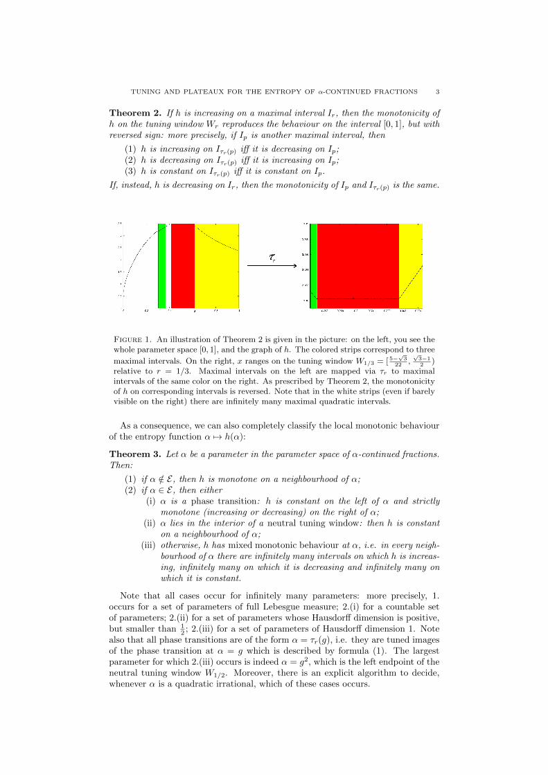
Theorem 2. If h is increasing on a maximal interval Ir, then the monotonicity ofh on the tuning window Wr reproduces the behaviour on the interval [0, 1], but withreversed sign: more precisely, if Ip is another maximal interval, then

(1) h is increasing on Iτr(p) iff it is decreasing on Ip;(2) h is decreasing on Iτr(p) iff it is increasing on Ip;(3) h is constant on Iτr(p) iff it is constant on Ip.

If, instead, h is decreasing on Ir, then the monotonicity of Ip and Iτr(p) is the same.

Figure 1. An illustration of Theorem 2 is given in the picture: on the left, you see thewhole parameter space [0, 1], and the graph of h. The colored strips correspond to three

maximal intervals. On the right, x ranges on the tuning window W1/3 = [ 5−√3

22,√3−12

)relative to r = 1/3. Maximal intervals on the left are mapped via τr to maximalintervals of the same color on the right. As prescribed by Theorem 2, the monotonicityof h on corresponding intervals is reversed. Note that in the white strips (even if barelyvisible on the right) there are infinitely many maximal quadratic intervals.

As a consequence, we can also completely classify the local monotonic behaviourof the entropy function α 7→ h(α):

Theorem 3. Let α be a parameter in the parameter space of α-continued fractions.Then:

(1) if α /∈ E, then h is monotone on a neighbourhood of α;(2) if α ∈ E, then either

(i) α is a phase transition: h is constant on the left of α and strictlymonotone (increasing or decreasing) on the right of α;

(ii) α lies in the interior of a neutral tuning window: then h is constanton a neighbourhood of α;

(iii) otherwise, h has mixed monotonic behaviour at α, i.e. in every neigh-bourhood of α there are infinitely many intervals on which h is increas-ing, infinitely many on which it is decreasing and infinitely many onwhich it is constant.

Note that all cases occur for infinitely many parameters: more precisely, 1.occurs for a set of parameters of full Lebesgue measure; 2.(i) for a countable setof parameters; 2.(ii) for a set of parameters whose Hausdorff dimension is positive,but smaller than 1

2 ; 2.(iii) for a set of parameters of Hausdorff dimension 1. Notealso that all phase transitions are of the form α = τr(g), i.e. they are tuned imagesof the phase transition at α = g which is described by formula (1). The largestparameter for which 2.(iii) occurs is indeed α = g2, which is the left endpoint of theneutral tuning window W1/2. Moreover, there is an explicit algorithm to decide,whenever α is a quadratic irrational, which of these cases occurs.


The structure of the paper is as follows. In section 2, we introduce basic notationand definitions about continued fractions, and in section 3 we recall the constructionand results from [CT] which are relevant in this paper. We then define the tuningoperators and establish their basic properties (section 4), and discuss the behaviourof tuning with respect to monotonicity of entropy, thus proving Theorem 2 (section5). In section 6 we discuss untuned and dominant parameters, and use them toprove the characterization of plateaux (Theorem 1 above, and Theorem 37). Finally,section 7 is devoted to the proof of Theorem 3.

2. Background and definitions

2.1. Continued fractions. The continued fraction expansion of a number

x =1

a1 + 1a2+...

will be denoted by x = [0; a1, a2, . . . ], and the nth convergent of x will be denotedby pn

qn:= [0; a1, ..., an]. Often we will also use the compact notation x = [0;S] where

S = (a1, a2, . . . ) is the (finite or infinite) string of partial quotients of x.If S is a finite string, its length will be denoted by |S|. A string A is a prefix of

S if there exists a (possibly empty) string B such that S = AB; A is a suffix of Sif there exists a (possibly empty) string B such that S = BA; A is a proper suffixof S if there exists a non-empty string B such that S = BA.

Definition 4. Let S = (s1, . . . , sn), T = (t1, . . . , tn) be two strings of positiveintegers of equal length. We say that S < T if there exists 0 ≤ k < n such that

si = ti ∀1 ≤ i ≤ k and

{sk+1 < tk+1 if k is oddsk+1 > tk+1 if k is even

This is a total order on the set of strings of given length, and it is defined sothat S < T iff [0;S] < [0;T ]. As an example, (2, 1) < (1, 1) < (1, 2). Moreover, thisorder can be extended to a partial order on the set of all finite strings of positiveintegers in the following way:

Definition 5. If S = (s1, . . . , sn), T = (t1, . . . , tm) are strings of finite (not neces-sarily equal) length, then we define S << T if there exists 0 ≤ k < min{n,m} suchthat

si = ti ∀1 ≤ i ≤ k and

{sk+1 < tk+1 if k is oddsk+1 > tk+1 if k is even

As an example, (2, 1) << (1), and (2, 1, 2) << (2, 2). This order has the followingproperties:

(1) if |S| = |T |, then S < T if and only if S << T ;(2) if X,Y are infinite strings and S << T , then [0;SX] < [0;TY ];(3) if A ≤ B and B << C, then A << C.

2.2. Fractal sets defined by continued fractions. We can define an action ofthe semigroup of finite strings (with the operation of concatenation) on the unitinterval. Indeed, for each S, we denote by S · x the number obtained by appendingthe string S at the beginning of the continued fraction expansion of x; by conventionthe empty string corresponds to the identity.

We shall also use the notation fS(x) := S · x; let us point out that the Gaussmap G(x) :=

{1x

}acts as a shift on continued fraction expansions, hence fS is a

right inverse of G|S| (G|S| ◦ fS(x) = x). It is easy to check that concatenation ofstrings corresponds to composition (ST ) · x = S · (T · x); moreover, the map fS is


increasing if |S| is even, decreasing if it is odd. It is not hard to see that fS is givenby the formula

(3) fS(x) =pn−1x+ pnqn−1x+ qn

where pnqn

= [0; a1, . . . , an] and pn−1

qn−1= [0; a1, . . . , an−1]. The map fS is a contraction

of the unit interval: indeed, by taking the derivative in the previous formula and

using the relation qnpn−1 − pnqn−1 = (−1)n (see [IK]), f ′S(x) = (−1)n(qn−1x+qn)2

, hence

(4)1

4q(S)2≤ |f ′S(x)| ≤ 1

q(S)2∀x ∈ [0, 1]

where q(S) = qn is the denominator of the rational number whose c.f. expansion isS.

A common way of defining Cantor sets via continued fraction expansions is thefollowing:

Definition 6. Given a finite set A of finite strings of positive integers, the regularCantor set defined by A is the set

K(A) := {x = [0;W1,W2, . . . ] : Wi ∈ A ∀i ≥ 1}

For instance, the case when the alphabet A consists of strings with a single digitgives rise to sets of continued fractions with restricted digits [He].

An important geometric invariant associated to a fractal subset K of the realline is its Hausdorff dimension H.dim K. In particular, a regular Cantor set isgenerated by an iterated function system, and its dimension can be estimated in astandard way (for basic properties about Hausdorff dimension we refer to Falconer’sbook [Fa], in particular Chapter 9).

Indeed, if the alphabet A = {S1, . . . , Sk} is not redundant (in the sense that noSi is prefix of any Sj with i 6= j), the dimension of K(A) is bounded in terms ofthe smallest and largest contraction factors of the maps fW ([Fa], Proposition 9.6):

(5)logN

− logm1≤ H.dim K(A) ≤ logN

− logm2

where m1 := inf W∈Ax∈[0,1]

|f ′W (x)|, m2 := sup W∈Ax∈[0,1]

|f ′W (x)|, and N is the cardinality

of A.

3. Matching intervals

Let us now briefly recall the main construction of [CT], which will be essentialin the following.

Each irrational number has a unique infinite continued fraction expansions, whileevery rational number has exactly two finite expansions. In this way, one canassociate to every rational r ∈ Q ∩ (0, 1) two finite strings of positive integers: letS0 be the string of even length, and S1 be the one of odd length. For instance, since3/10 = [0; 3, 3] = [0; 3, 2, 1], the two strings associated to 3/10 will be S0 = (3, 3)and S1 = (3, 2, 1). Let us remark that, if r = [0;S0] = [0;S1] then S0 >> S1.

Now, for each r ∈ Q ∩ (0, 1) we define the quadratic interval associated to r asthe open interval

Ir := (α1, α0)

whose endpoints are the two quadratic irrationals α0 = [0;S0] and α1 = [0;S1]. Itis easy to check that r always belongs to Ir, and it is the unique element of Q ∩ Irwhich is a convergent of both endpoints of Ir. In fact r is the rational with minimaldenominator in Ir, and it will be called the pseudocenter of Ir. Let us define thebifurcation set (or exceptional set in the terminology of [CT]) as


(6) E := [0, g] \⋃

r∈(0,1)∩Q

Ir

The intervals Ir will often overlap; however, by ([CT], Prop. 2.4 and Lemma2.6), the connected components of [0, g]\E are themselves quadratic intervals, calledmaximal quadratic intervals. That is to say, every quadratic interval is contained ina unique maximal quadratic interval, and two distinct maximal quadratic intervalsdo not intersect. This way, the set of pseudocenters of maximal quadratic intervalsis a canonically defined subset of Q ∩ (0, 1) and will be denoted by

QE := {r ∈ (0, 1) : Ir is maximal}We shall sometimes refer to QE as the set of extremal rational values; this is moti-vated by the following characterization of QE :

Proposition 7 ([CT], Proposition 4.5). A rational number r = [0;S] belongs toQE if and only if, for any splitting S = AB of S into two strings A, B of positivelength, either

AB < BA

or A = B with |A| odd.

Using this criterion, for instance, one can check that [0; 3, 2] belongs to QE(because (3, 2) < (2, 3)), and so does [0; 3, 3], while [0; 2, 2, 1, 1] does not (indeed,(2, 1, 1, 2) < (2, 2, 1, 1)). Related to the criterion is the following characterizationof E in terms of orbits of the Gauss map G:

Proposition 8 ([BCIT], Lemma 3.3).

E = {x ∈ [0, 1] : Gk(x) ≥ x ∀k ∈ N}.

For t ∈ (0, 1) fixed, let us also define the closed set

B(t) := {x ∈ [0, 1] : Gk(x) ≥ t ∀k ∈ N}.To get a rough idea of the meaning of the sets B(t) let us mention that for t =1/(N + 1) one gets the set of values whose continued fraction expansion is infiniteand contains only the digits {1, ..., N} as partial quotients. A simple relation followsfrom the definitions:

Remark 9. For each t ∈ [0, 1], E ∩ [t, 1] ⊆ B(t).

A thorough study of the sets B(t) and their interesting connection with E iscontained in [CT2]. Note that, from Remark 9 and ergodicity of the Gauss map, itfollows that the Lebesgue measure of E is zero.

3.1. Maximal intervals and matching. Let us now relate the previous construc-tion to the dynamics of α-continued fractions. The main result of [CT] is that forall parameters α belonging to a maximal quadratic interval Ir, the orbits of α andα−1 under the α-continued fraction transformation Tα coincide after a finite num-ber of steps, and this number of steps depends only on the usual continued fractionexpansion of the pseudocenter r:

Theorem 10 ([CT], Thm 3.1). Let Ir be a maximal quadratic interval, and r =[0; a1, . . . , an] with n even. Let

(7) N =∑i even

ai M =∑i odd

ai

Then for all α ∈ Ir,(8) TN+1

α (α) = TM+1α (α− 1)


Equation (8) is called matching condition. Notice that N and M are the samefor all α which belong to the open interval Ir. Indeed, even more is true, namely thesymbolic orbits of α and α− 1 up to steps respectively N and M are constant overall the interval Ir ([CT], Lemma 3.7). Thus we can regard each maximal quadraticinterval as a stability domain for the family of α-continued fraction transformations,and the complement E as the bifurcation locus.

One remarkable phenomenon, which was first discovered by Nakada and Natsui([NN], Thm. 2), is that the matching condition locally determines the monotonicbehaviour of h(α):

Proposition 11 ([CT], Proposition 3.8). Let Ir be a maximal quadratic interval,and let N,M be as in Theorem 10. Then:

(1) if N < M , the entropy h(α) is increasing for α ∈ Ir;(2) if N = M it is constant on Ir;(3) if N > M it is decreasing on Ir.

4. Tuning

Let us now define tuning operators acting on parameter space, inspired by thedictionary with complex dynamics (see the Appendix). We will then see how suchoperators are responsible for the self-similar structure of the entropy.

4.1. Tuning windows. Let r ∈ QE be the pseudocenter of the maximal intervalIr = (α1, α0); if r = [0;S0] = [0;S1] are the even and odd expansions of r, thenαi = [0;Si] (i = 0, 1). Let us also set ω := [0;S1S0] and define the tuning windowgenerated by r as the interval

Wr := [ω, α0).

The value α0 will be called the root of the tuning window. For instance, if r = 12 =

[0; 2] = [0; 1, 1], then ω = [0; 2, 1] = g2 and the root α0 = [0; 1] = g.The following proposition describes in more detail the structure of the tuning

windows: a value x belongs to B(ω)∩ [ω, α0] if and only if its continued fraction isan infinite concatenation of the strings S0, S1.

Proposition 12. Let r ∈ QE, and let Wr = [ω, α0). Then

B(ω) ∩ [ω, α0] = K(Σ)

where K(Σ) is the regular Cantor set on the alphabet Σ = {S0, S1}.

For instance, if r = 12 , then W 1

2= [g2, g), and B(g2) ∩ [g2, g] is the set of

numbers whose continued fraction expansion is an infinite concatenation of thestrings S0 = (1, 1) and S1 = (2).

4.2. Tuning operators. For each r ∈ QE we can define the tuning map τr :[0, 1]→ [0, r] as τr(0) = ω and

(9) τr([0; a1, a2, . . . ]) = [0;S1Sa1−10 S1S

a2−10 . . . ]

Note that this map is well defined even on rational values (where the continued frac-tion representation is not unique); for instance, τ1/3([0; 3, 1]) = [0; 3, 2, 1, 2, 1, 3] =[0; 3, 2, 1, 2, 1, 2, 1] = τ1/3([0; 4]).

It will be sometimes useful to consider the action that τr induces on finite stringsof positive integers: with a slight abuse of notation we shall denote this action bythe same symbol τr.

Lemma 13. For each r ∈ QE, the map τr is strictly increasing (hence injective).Moreover, τr is continuous at all irrational points, and discontinuous at every pos-itive rational number.


The first key feature of tuning operators is that they map the bifurcation setinto a small copy of itself:

Proposition 14. Let r ∈ QE. Then

(i) τr(E) = E ∩Wr, and τr is a homeomorphism of E onto E ∩Wr;(ii) τr(QE) = QE ∩Wr \ {r}.

Let us moreover notice that tuning windows are nested:

Lemma 15. Let r, s ∈ QE. Then the following are equivalent:

(i) Wr ∩Ws 6= ∅ with r < s;(ii) r = τs(p) for some p ∈ QE;(iii) Wr ⊆Ws.

4.3. Proofs.

Proof of lemma 13. Let us first prove that τr preserves the order between irrationalnumbers. Pick α, β ∈ (0, 1) \Q, α 6= β. Then

α := [0;P, a, a2, a3, ...], β := [0;P, b, b2, b3, ...]

where P is a finite string of positive integers (common prefix), and we may assumealso that a < b. Then

τr(α) := [0; τr(P ), S1, Sa−10 , S1, ...], τr(β) := [0; τr(P ), S1, S

b−10 , S1, ...].

Since |Sa−10 | is even and S1 << S0, we get Sa−10 S1 << Sb−10 S1, whence S1Sa−10 S1 >>

S1Sb−10 S1. Therefore, since |P | ≡ |τr(P )| mod 2, we get that either |P | is even,

α > β and τr(α) > τr(β), or |P | is odd , α < β and τr(α) < τr(β), so we are done.The continuity of τr at irrational points follows from the fact that if β ∈ (0, 1) \Qand x is close to β then the continued fraction expansions of x and β have a longcommon prefix, and, by definition of τr, then their images will also have a longprefix in common, and will therefore be close to each other. Finally, let us checkthat the function is increasing at each rational number c > 0. This follows fromthe property:

(10) supα∈R\Qα<c

τr(α) < τr(c) < infα∈R\Qα>c

τr(α)

Let us prove the left-hand side inequality of (10) (the right-hand side one hasessentially the same proof). Suppose c = [0;S], with |S| ≡ 1 mod 2. Then everyirrational α < c has an expansion of the form α = [0;S,A] with A an infinitestring. Hence τr(α) = [0; τr(S), τr(A)], and it is not hard to check that sup τr(α) =[0; τr(S), S1, S0] < [0; τr(S)] = τr(c). Discontinuity at positive rational points alsofollows from (10). �

To prove Propositions 12 and 14 we first need some lemmata.

Lemma 16. Let r = [0;S0] = [0;S1] ∈ QE and y be an irrational number with c.f.expansion y = [0;B,S∗, . . . ], where B is a proper suffix of either S0 or S1, and S∗equal to either S0 or S1. Then y > [0;S1].

Proof. If B = (1) then there is hardly anything to prove (by Prop. 7, the first digitof S1 is strictly greater than 1). If not, then one of the following is true:

(1) S0 = AB and A is a prefix of S1 as well;(2) S1 = AB and A is a prefix of S0 as well.

By Prop. 7, in the first case we get that BA ≥ AB = S0 >> S1, while in the latterBA >> AB = S1; so in both cases BA >> S1 and the claim follows. �


Lemma 17. Let r ∈ QE, and x, y ∈ [0, 1] \Q. Then

Gk(x) ≥ y ∀k ≥ 0

if and only ifGk(τr(x)) ≥ τr(y) ∀k ≥ 0

Proof. Since τr is increasing, Gk(x) ≥ y if and only if τr(Gk(x)) ≥ τr(y) if and only

if GNk(τr(x)) ≥ τr(y) for Nk = |S0|(a1 + · · ·+ ak) + (|S1| − |S0|)k.On the other hand, if h is not of the form Nk, Gh(τr(x)) = [0;B,S∗, . . . ] with B

a proper suffix of either S0 or S1, and S∗ equal to either S0 or S1. By Lemma 16it follows immediately that

Gh(τr(x)) > [0;S1] ≥ τr(y)

�

Proof of Proposition 12. Let us first prove that, if x ∈ B(ω)∩ [ω, α0] then x = S · ywith y ∈ B(ω) ∩ [ω, α0] and S ∈ {S0, S1}; then the inclusion

B(ω) ∩ [ω, α0] ⊂ K(Σ)

will follow by induction. If x ∈ B(ω) ∩ [ω, α0] then the following alternative holds

(x > r) x = S0 · y and S0 · y = x < α0 = S0 · α0, therefore y ≤ α0;(x < r) x = S1 · y and S1 · y = x > ω = S1 · α0, therefore y ≤ α0;

Note that, since the map y 7→ S · y preserves or reverses the order depending onthe parity of |S|, in both cases we get to the same conclusion. Moreover, sinceB(ω) is forward-invariant with respect to the Gauss map and x ∈ B(ω), theny = Gk(x) ∈ B(ω) as well, hence y ∈ B(ω) ∩ [ω, α0].

To prove the other inclusion, let us first remark that every x ∈ K(Σ) satisfiesω ≤ x ≤ α0. Now, let k ∈ N; either Gk(x) ∈ K(Σ), and hence Gk(x) ≥ ω, orGk(x) = [0;B,S∗, ...] satisfies the hypotheses of Lemma 16, and hence we get thaty > [0;S1] > ω. Since Gk(x) ≥ ω holds for any k, then x ∈ B(ω). �

Proof of Proposition 14. (i) Recall the notation Wr = [ω, α0), and let v ∈ E ∩Wr.By Remark 9, E ∩ Wr ⊆ B(ω) ∩ [ω, α0), hence, by Proposition 12, v ∈ K(Σ).Moreover, v < r because E ∩ [r, α0) = ∅. As a consequence, the c.f. expansion ofv is an infinite concatenation of strings in the alphabet {S0, S1} starting with S1.Now, if the expansion of v terminates with S0, then Gk(v) = ω for some k, hence vmust coincide with ω = [0;S1S0], so v = τr(0) and we are done. Otherwise, thereexists some x ∈ [0, 1) such that v = τr(x): then by Lemma 17 we get that

Gk(v) ≥ v ∀k ≥ 0⇒ Gk(x) ≥ x ∀k ≥ 0

which means x belongs to E .Viceversa, let us pick x := τr(v) with v ∈ E . By definition of τr, x ∈ Wr.

Moreover, since v belongs to E , Gn(v) ≥ v for any n, hence by Lemma 17 also τr(v)belongs to E . The fact that τr is a homeomorphism follows from bijectivity andcompactness.

(ii) Let p ∈ QE and Ip = (α1, α0) the maximal quadratic interval generated byp; by point (i) above also the values βi := τr(αi), (i = 0, 1) belong to E ∩ Wr.Since τr is strictly increasing, no other point of E lies between β1 and β0, hence(β1, β0) = Is for some s ∈ QE ∩ [ω, r). Since τr(p) is a convergent to both τr(α0)and τr(α1), then τr(p) = s.

To prove the converse, pick s ∈ QE ∩ [ω, r) and denote Is = (β1, β0). Againby point (i), βi := τr(αi) for some α0, α1 ∈ E , and (α1, α0) is a component ofthe complement of E , hence there exists p ∈ QE such that Ip = (α1, α0). As aconsequence, s = τr(p). �


Proof of lemma 15. Let us denote Ws = [ω(s), α0(s)), Wr = [ω(r), α0(r)), Wp =[ω(p), α0(p)). Suppose (i): then, since the closures of Wr and Ws are not disjoint,ω(s) ≤ α0(r). Moreover, ω(s) ∈ E and E ∩ (r, α0(r)] = {α0(r)}, hence ω(s) ≤ r be-cause ω(s) cannot coincide with α0(r), not having a purely periodic c.f. expansion.Hence r ∈Ws and, by Proposition 14, there exists p ∈ QE such that r = τs(p).

Suppose now (ii). Then, since r = τs(p), also α0(r) = τs(α0(p)) ≤ s < α0(s),and ω(r) = τs(ω(p)) ∈Ws, which implies (iii).

(iii) ⇒ (i) is clear. �

5. Tuning and monotonicity of entropy: proof of Theorem 2

Definition 18. Let A = (a1, ..., an) be a string of positive integers. Then itsmatching index JAK is the alternating sum of its digits:

(11) JAK :=

n∑j=1

(−1)j+1aj

Moreover, if r = [0;S0] is a rational number between 0 and 1 and S0 is its continuedfraction expansion of even length, we define the matching index of r to be

JrK := JS0K

The reason for this terminology is the following. Suppose r ∈ QE is the pseu-docenter of the maximal quadratic interval Ir: then by Theorem 10, a matchingcondition (8) holds, and by formula (7)

(12) JrK =

n∑j=1

(−1)j+1aj = M −N

where r = [0;S0] and S0 = (a1, . . . , an). This means, by Proposition (11), that theentropy function h(α) is increasing on Ir iff JrK > 0, decreasing on Ir iff JrK < 0,and constant on Ir iff JrK = 0.

Lemma 19. Let r, p ∈ QE. Then

(13) Jτr(p)K = −JrKJpK.

Proof. The double bracket notation behaves well under concatenation, namely:

JABK :=

{JAK + JBK if |A| evenJAK− JBK if |A| odd

Let p = [0; a1, ..., an] and r = [0;S0] be the continued fraction expansions of evenlength of p, r ∈ QE ; using the definition of τr we get

Jτr(p)K =

n∑j=1

(−1)j+1 (JS1K− (aj − 1)JS0K)

and, since n = |A| is even, the right-hand side becomes JS0K∑nj=1(−1)jaj , whence

the thesis. �

Definition 20. A quadratic interval Ir is called neutral if JrK = 0. Similarly, atuning window Wr is called neutral if JrK = 0.

As an example, the rational r = 12 = [0; 2] = [0; 1, 1] generates the neutral tuning

window W1/2 = [g2, g).

Proof of Theorem 2. Let Ir be a maximal quadratic interval over which theentropy is increasing. Then, by Theorem 10 and Proposition 11, for α ∈ Ir, amatching condition (8) holds, with M −N > 0. This implies by (12) that JrK > 0.


Let now Ip be another maximal quadratic interval. By Proposition 14 (ii), Iτr(p) isalso a maximal quadratic interval, and by Lemma 19

Jτr(p)K = −JrKJpK

Since JrK > 0, then Jτr(p)K and JpK have opposite sign. In terms of the monotonicityof entropy, this means the following:

(1) if the entropy is increasing on Ip, then by (12) JpK > 0, hence Jτr(p)K < 0,which implies (again by (12)) that the entropy is decreasing on Iτr (p);

(2) if the entropy is decreasing on Ip, then JpK < 0, hence Jτr(p)K > 0 and theentropy is increasing on Iτr (p);

(3) if the entropy is constant on Ip, then JpK = 0, hence Jτr(p)K = 0 and theentropy is constant on Iτr (p).

If, instead, the entropy is decreasing on Ir, then JrK > 0, hence Jτr(p)K and JpK havethe same sign, which similarly to the previous case implies that the monotonicityof entropy on Ip and Iτr(p) is the same. �

Remark 21. The same argument as in the proof of Theorem 2 shows that, ifr ∈ QE with JrK = 0, then the entropy on Iτr(p) is constant for each p ∈ QE (nomatter what the monotonicity is on Ip).

6. Plateaux: proof of Theorem 1

The goal of this section is to prove Theorem 37, which characterizes the plateauxof the entropy and has as a consequence Theorem 1 in the introduction. Meanwhile,we introduce the sets of untuned parameters (subsection 6.2) and dominant param-eters (subsection 6.3) which we will use in the proof of the Theorem (subsection6.4).

6.1. The importance of being Holder. The first step in the proof of Theorem1 is proving that the entropy function h(α) is indeed constant on neutral tuningwindows:

Proposition 22. Let r ∈ QE generate a neutral maximal interval, i.e. JrK = 0.Then the entropy function h(α) is constant on Wr.

By Remark 21, we already know that the entropy is locally constant on allconnected components of Wr \ E , which has full measure in Wr. However, sinceWr ∩ E has, in general, positive Hausdorff dimension, in order to prove that theentropy is actually constant on the whole Wr one needs to exclude a devil staircasebehaviour. We shall exploit the following criterion:

Lemma 23. Let f : I → R be a Holder-continuous function of exponent η ∈ (0, 1),and assume that there exists a closed set C ⊆ I such that f is locally constant atall x /∈ C. Suppose moreover H.dim C < η. Then f is constant on I.

Proof. Suppose f is not constant: then by continuity f(I) is an interval with non-empty interior, hence H.dim f(I) = 1. On the other hand, we know f is constanton the connected components of I \ C, so we get f(I) = f(C), whence

H.dim f(C) = H.dim f(I) = 1.

But, since f is η-Holder continuous, we also get (e.g. by [Fa], prop. 2.3)

H.dim f(C) ≤ H.dim C

η

and thus η ≤ H.dim C, contradiction. �

Let us know check the hypotheses of Lemma 23 are met in our case; the first oneis given by the following


Theorem 24 ([Ti]). For all fixed 0 < η < 1/2, the function α 7→ h(α) is locallyHolder-continuous of exponent η on (0, 1].

We are now left with checking that the Hausdorff dimension of E ∩Wr is smallenough:

Lemma 25. For all r ∈ QE,

H.dim E ∩Wr ≤log 2

log 5< 1/2.

Proof. Let r ∈ QE , r = [0;S0] = [0;S1] and Wr = [ω, α]. By Remark 9 andProposition 12,

E ∩Wr ⊂ B(ω) ∩ [ω, α] = K(Σ), with Σ = {S0, S1}.Note we also have K(Σ) = K(Σ2) with Σ2 = {S0S0, S1S0, S1S0, S1S1} and, byvirtue of (4) we have the estimate

|f ′SiSj (x)| ≤ 1

q(SiSj)2, i, j ∈ {0, 1}.

On the other hand, setting Z0 = (1, 1) and Z1 = (2) we can easily check that

q(SiSj) ≥ q(ZiZj) = 5 ∀i, j ∈ {0, 1};

whence |f ′SiSj (x)| ≤ 125 and, by formula (5), we get our claim. �

Proposition 22 now follows from Lemma 23, Theorem 24 and Lemma 25.

6.2. Untuned parameters. The set of untuned parameters is the complement ofall tuning windows:

UT := [0, g] \⋃

r∈Q∩(0,1)

Wr

Note that, since Ir ⊆ Wr, UT ⊆ E . Moreover, we say that a rational a ∈ QEis untuned if it cannot be written as a = τr(a0) for some r, a0 ∈ QE . We shalldenote by QUT the set of all a ∈ QE which are untuned. Let us start out byseeing that each pseudocenter of a maximal quadratic interval admits an “untunedfactorization”:

Lemma 26. Each r ∈ QE can be written as:

(14) r = τrm ◦ · · · ◦ τr1(r0), with ri ∈ QUT ∀i ∈ {0, 1, ...,m}.Note that m can very well be zero (when r is already untuned).

Proof. A straightforward check shows that the tuning operator has the followingassociativity property:

(15) ττp(r)(x) = τp ◦ τr(x) ∀p, r ∈ QE , x ∈ (0, 1)

For s = [0; a1, ..., am] ∈ QE we shall set ‖s‖1 :=∑m

1 ai; this definition does notdepend on the representation of s, moreover

‖τp(s)‖1 = ‖p‖1‖s‖1 ∀p, s ∈ QEThe proof of (14) follows then easily by induction on N = ‖r‖1, using the fact thatmax(‖p‖1, ‖s‖1) ≤ ‖τp(s)‖1/2. �

As a consequence of the following proposition, the connected components of thecomplement of UT are precisely the tuning windows generated by the elements ofQUT :

Proposition 27. The set UT is a Cantor set: indeed,


(i)

UT = [0, g] \⋃

r∈QUT

Wr;

(ii) if r, s ∈ QUT with r 6= s, then Wr and Ws are disjoint;(iii) if x ∈ UT \ UT , then there exists r ∈ QUT such that x = τr(0).

Proof. (i). It is enough to prove that every tuning window Wr is contained in atuning window Ws, with s ∈ QUT . Indeed, let r ∈ QE ; either r ∈ QUT or, byLemma 26, there exists p ∈ QE and s ∈ QUT such that r = τs(p), hence Wr ⊆Ws.

(ii). By Lemma 15, if the closures of Wr and Ws are not disjoint, then r = τs(p),which contradicts the fact r ∈ QUT .

(iii). By (i) and (ii), UT is a Cantor set, and each element x which belongs toUT \ UT is the left endpoint of some tuning window Wr with r ∈ QUT , which isequivalent to say x = τr(0). �

Lemma 28. The Hausdorff dimension of UT is full:

H.dim UT = 1

Proof. By the properties of Hausdorff dimension,

H.dim E = max{H.dim UT, supr∈QUT

H.dim E ∩Wr}

Now, by [CT], H.dim E = 1, and, by Lemma 25, H.dim E ∩Wr <12 , hence the

claim. �

6.3. Dominant parameters.

Definition 29. A finite string S of positive integers is dominant if it has evenlength and

S = AB << B

for any splitting S = AB of S into two non-empty strings A, B.

That is to say, dominant strings are smaller than all their proper suffixes. Arelated definition is the following:

Definition 30. A quadratic irrational α ∈ [0, 1] is a dominant parameter if its c.f.expansion is of the form α = [0;S] with S a dominant string.

For instance, (2, 1, 1, 1) is dominant, while (2, 1, 1, 2) is not (it is not true that(2, 1, 1, 2) << (2)). In general, all strings whose first digit is strictly greater thanthe others are dominant, but there are even more dominant strings (for instance(3, 1, 3, 2) is dominant).

Remark 31. By Proposition 7, if S is dominant then [0;S] ∈ QE.

A very useful feature of dominant strings is that they can be easily used toproduce other dominant strings:

Lemma 32. Let S0 be a dominant string, and B a proper suffix of S0 of evenlength. Then, for any m ≥ 1, Sm0 B is a dominant string.

Proof. Let Y be a proper suffix of Sm0 B. There are three possible cases:

(1) Y is a suffix of B, hence a proper suffix of S0. Hence, since S0 is dominant,S0 >> Y and Sm0 B >> Y .

(2) Y is of the form Sk0B, with 1 ≤ k < m. Then by dominance S0 >> B,

which implies Sm−k0 B >> B, hence Sm0 B >> Sk0B.(3) Y is of the form CSk0B, with 0 ≤ k < m and C a proper suffix of S0. Then

again the claim follows by the fact that S0 is dominant, hence S0 >> C.


�

Lemma 33. A dominant string S0 cannot begin with two equal digits.

Proof. By definition of dominance, S0 cannot consist of just k ≥ 2 equal digits.Suppose instead it has the form S0 = (a)kB with k ≥ 2 and B non empty andwhich does not begin with a. Then by dominance (a)kB << B, hence a << Bsince B does not begin with a. However, this implies aB << aa and hence aB <<(a)kB = S0, which contradicts the definition of dominance because aB is a propersuffix of S0. �

The reason why dominant parameters turn out to be so useful is that they canapproximate untuned parameters:

Proposition 34 ([CT2], Proposition 6). The set of dominant parameters is densein UT \ {g}. More precisely, every parameter in UT \ {g} is accumulated from theright by a dominant parameter.

Proposition 35. Every element β ∈ UT \{g} is accumulated by non-neutral max-imal quadratic intervals.

Proof. We shall prove that either β ∈ UT \ {g}, and β is accumulated from theright by non-neutral maximal quadratic intervals, or β = τs(0) for some s ∈ QUT ,and β is accumulated from the left by non-neutral maximal quadratic intervals.

If β ∈ UT then, by Proposition 34, β is the limit point from the right of asequence αn = [0;An] with An dominant. If JAnK 6= 0 for infinitely many n, theclaim is proven. Otherwise, it is sufficient to prove that every dominant parameterαn such that JAnK = 0 is accumulated from the right by non-neutral maximalintervals. Let S0 be a dominant string, with JS0K = 0, and let α := [0;S0]. Firstof all, the length of S0 is bigger than 2: indeed, if S0 had length 2, then conditionJS0K = 0 would force it to be of the form S0 = (a, a) for some a, which contradictsthe definition of dominant. Hence, we can write S0 = AB with A of length 2and B of positive, even length. Then, by Lemma 32, Sm0 B is also dominant,hence pm := [0;Sm0 B] ∈ QE by Remark 31. Moreover, α < pm since S0 << B.Furthermore, S0 cannot begin with two equal digits (Lemma 33), hence JAK 6= 0and JSm0 BK = JBK = JS0K − JAK 6= 0. Thus the sequence Ipm is a sequence ofnon-neutral maximal quadratic intervals which tends to β from the right, and theclaim is proven.

If β ∈ UT \ UT , then by Proposition 27 (iii) there exists s ∈ QUT such thatβ = τs(0). Since UT is a Cantor set and β lies on its boundary, β is the limit point(from the left) of a sequence of points of UT , hence the claim follows by the abovediscussion. �

6.4. Characterization of plateaux.

Definition 36. A parameter x ∈ E is finitely renormalizable if it belongs to finitelymany tuning windows. This is equivalent to say that x = τr(y), with y ∈ UT . Aparameter x ∈ E is infinitely renormalizable if it lies in infinitely many tuningwindows Wr, with r ∈ QE. Untuned parameters are also referred to as non renor-malizable.

We are finally ready to prove Theorem 1 stated in the introduction, and indeedthe following stronger version:

Theorem 37. An open interval U ⊆ [0, 1] of the parameter space of α-continuedfraction transformations is a plateau for the entropy function h(α) if and only if

it is the interior of a neutral tuning window U =◦Wr, with r of either one of the

following types:


(NR) r ∈ QUT , JrK = 0 (non-renormalizable case)

(FR) r = τr1(r0) with

{r0 ∈ QUT , Jr0K = 0r1 ∈ QE , Jr1K 6= 0

(finitely renormalizable case)

Proof. Let us pick r which satisfies (NR), and letWr = [ω, α0) be its tuning window.By Proposition 22, since JrK = 0, the entropy is constant on Wr. Let us prove thatit is not constant on any larger interval. Since r ∈ QUT , by Proposition 27, α0

belongs to UT . If α0 = g, then by the explicit formula (1) the entropy is decreasingto the right of α0. Otherwise, by Proposition 35, α0 is accumulated from theright by non-neutral maximal quadratic intervals, hence entropy is not constant tothe right of α0. Moreover, by Proposition 27, ω belongs to the boundary of UT ,hence, by Proposition 35, it is accumulated from the left by non-neutral intervals.This means that the interior of Wr is a maximal open interval of constance for theentropy h(α), i.e. a plateau.

Now, suppose that r satisfies condition (FR), with r = τr1(r0). By the (NR)case, the interior of Wr0 is a plateau, and Wr0 is accumulated from both sides bynon-neutral intervals. Since τr1 maps non-neutral intervals to non-neutral intervalsand is continuous on E , then Wr is accumulated from both sides by non-neutralintervals, hence its interior is a plateau.

Suppose now U is a plateau. Since E has no interior part (e.g. by formula (6)),there is r ∈ QE such that Ir intersects U , hence, by Proposition 11, JrK = 0 andactually Ir ⊆ U . Then, by Lemma 26 one has the factorization

r = τrn ◦ · · · ◦ τr1(r0)

with each ri ∈ QUT untuned (recall n can possibly be zero, in which case r = r0).Since the matching index is multiplicative (eq. (13)), there exists at least oneri with zero meatching index: let j ∈ {0, . . . , n} be the largest index such thatJrjK = 0. If j = n, let s := rn: by the first part of the proof, the interior of Ws is aplateau, and it intersects U because they both contain r (by lemma 15, r belongs

to the interior of Ws), hence U =◦Ws, and we are in case (NR).

If, otherwise, j < n, let s := τrn ◦ · · · ◦ τrj+1(rj). By associativity of tuning (eq.

(15)) we can write

s = τs1(s0)

with s0 := rj and s1 := τrn ◦ · · · ◦ τrj+2(rj+1). Moreover, by multiplicativity of the

matching index (eq. (13)) Js1K 6= 0, hence s falls into the case (FR) and by the firstpart of the proof the interior of Ws is a plateau. Also, by construction, r belongsto the image of τs, hence it belongs to the interior of Ws. As a consequence, U and◦Ws are intersecting plateaux, hence they must coincide. �

7. Classification of local monotonic behaviour

Lemma 38. Any non-neutral tuning window Wr contains infinitely many intervalson which the entropy h(α) is constant, infinitely many over which it is increasing,and infinitely many on which it is decreasing.

Proof. Let us consider the following sequences of rational numbers

sn := [0;n, 1]

tn := [0;n, n]

un := [0;n+ 1, n, 1, n]

It is not hard to check (e.g. using Proposition 7) that sn, tn, un belong to QE .Moreover, by computing the matching indices one finds that, for n > 2, the entropy


h(α) is increasing on Isn , constant on Itn and decreasing on Iun . Since Wr is non-neutral, by Theorem 2 τr either induces the same monotonicity or the opposite one,hence the sequences Iτr(sn), Iτr(tn) and Iτr(un) are sequences of maximal quadraticintervals which lie in Wr and display all three types of monotonic behaviour. �

Proof of Theorem 3. Let α ∈ [0, 1] be a parameter. If α /∈ E , then α belongs tosome maximal quadratic interval Ir, hence h(α) is monotone on Ir by Proposition11, and by formula (12) the monotonicity type depends on the sign of JrK.

If α ∈ E , there are the following cases:

(1) α = g. Then α is a phase transition as described by formula (1);(2) α ∈ UT \ {g}. Then, by Proposition 35, α is accumulated from the right

by non-neutral tuning windows, and by Lemma 38 each non-neutral tuningwindow contains infinitely many intervals where the entropy is constant,increasing or decreasing; the parameter α has therefore mixed monotonicbeahaviour.

(3) α is finitely renormalizable. Then one can write α = τr(y), with y ∈ UT .There are three subcases:(3a) JrK 6= 0, and y = g. Since τr maps neutral intervals to neutral intervals

and non-neutral intervals to non-neutral intervals, the phase transitionat y = g gets mapped to a phase transition at α.

(3b) JrK 6= 0, and y 6= g. Then, by case (2) y is accumulated from the rightby intervals with all types of monotonicity, hence so is α.

(3c) If JrK = 0, then by using the untuned factorization (Lemma 26) onecan write

α = τrm ◦ · · · ◦ τr0(y) ri ∈ QUT

Let now j ∈ {0, . . . ,m} be the largest index such that JrjK = 0. Ifj = m, then α belongs to the neutral tuning window Wrm : thus,either α belongs to the interior of Wrm (which means by Proposition22 that the entropy is locally constant at α), or α coincides with theleft endpoint of Wrm . In the latter case, α belongs to the boundary ofUT , hence by Proposition 35 and Lemma 38 it has mixed behaviour.If j < m, then by the same reasoning as above τrj ◦ · · · ◦ τr0(y) eitherlies inside a plateau or has mixed behaviour, and since the operatorτrm ◦ · · · ◦ τrj+1 either respects the monotonicity or reverses it, also αeither lies inside a plateau or has mixed behaviour.

(4) α is infinitely renormalizable, i.e. α lies in infinitely many tuning windows.If α lies in at least one neutral tuning window Wr = [ω, α0), then it mustlie in its interior, because ω is not infinitely renormalizable. This means, byProposition 22, that h must be constant on a neighbourhood of α. Other-wise, α lies inside infinitely many nested non-neutral tuning windows Wrn .Since the sequence the denominators of the rational numbers rn must beunbounded, the size of Wrn must be arbitrarily small. By Lemma 38, ineach Wrn there are infinitely many intervals with any monotonicity typeand α displays mixed behaviour.

�Note that, as a consequence of the previous proof, α is a phase transition if and

only if it is of the form α = τr(g), with r ∈ QE and JrK 6= 0, hence the set of phasetransitions is countable. Moreover, the set of points of E which lie in the interiorof a neutral tuning window has Hausdorff dimension less than 1/2 by Lemma 25.

Finally, the set of parameters for which there is mixed behaviour has zeroLebesgue measure because it is a subset of E . On the other hand, it has full


Hausdorff dimension because such a set contains UT \ {g}, and by Lemma 28 UThas full Hausdorff dimension.

Appendix: Tuning for quadratic polynomials

The definition of tuning operators given in section 4 arises from the dictionarybetween α-continued fractions and quadratic polynomials first discovered in [BCIT].In this appendix, we will recall a few facts about complex dynamics and show howour construction is related to the combinatorial structure of the Mandelbrot set.

Tuning for quadratic polynomials. Let fc(z) := z2 + c be the family of qua-dratic polynomials, with c ∈ C. Recall the Mandelbrot set M is the set of param-eters c ∈ C such that the orbit of the critical point 0 is bounded under the actionof fc.

The Mandelbrot set has the remarkable property that near every point of itsboundary there are infinitely many copies of the whole M, called baby Mandelbrotsets. A hyperbolic component W of the Mandelbrot set is an open, connected subsetof M such that all c ∈ W , the orbit of the critical point fn(0) is attracted to aperiodic cycle.

Douady and Hubbard [DH] related the presence of baby copies of M to renor-malization in the family of quadratic polynomials. More precisely, they associatedto any hyperbolic component W a tuning map ιW :M→M which maps the maincardioid of M to W , and such that the image of the whole M under ιW is a babycopy of M.

External rays. A coordinate system on the boundary of M is given by externalrays. Indeed, the exterior of the Mandelbrot set is biholomorphic to the exterior ofthe unit disk

Φ : {z ∈ C : |z| > 1} → C \M

The external ray at angle θ is the image of a ray in the complement of the unitdisk:

R(θ) := Φ({ρe2πiθ : ρ > 1})

The ray at angle θ is said to land at c ∈ ∂M if limρ→1 Φ(ρe2πiθ) = c. This wayangles in R/Z determine parameters on the boundary of the Mandelbrot set, andit turns out that the binary expansions of such angles are related to the dynamicsof the map fc.

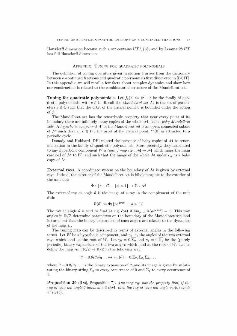
The tuning map can be described in terms of external angles in the followingterms. Let W be a hyperbolic component, and η0, η1 the angles of the two externalrays which land on the root of W . Let η0 = 0.Σ0 and η1 = 0.Σ1 be the (purelyperiodic) binary expansions of the two angles which land at the root of W . Let usdefine the map τW : R/Z→ R/Z in the following way:

θ = 0.θ1θ2θ3 . . . 7→ τW (θ) = 0.Σθ1Σθ2Σθ3 . . .

where θ = 0.θ1θ2 . . . is the binary expansion of θ, and its image is given by substi-tuting the binary string Σ0 to every occurrence of 0 and Σ1 to every occurrence of1.

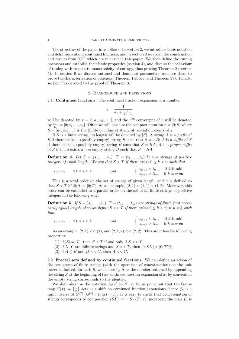
Proposition 39 ([Do], Proposition 7). The map τW has the property that, if theray of external angle θ lands at c ∈ ∂M, then the ray at external angle τW (θ) landsat ιW (c).


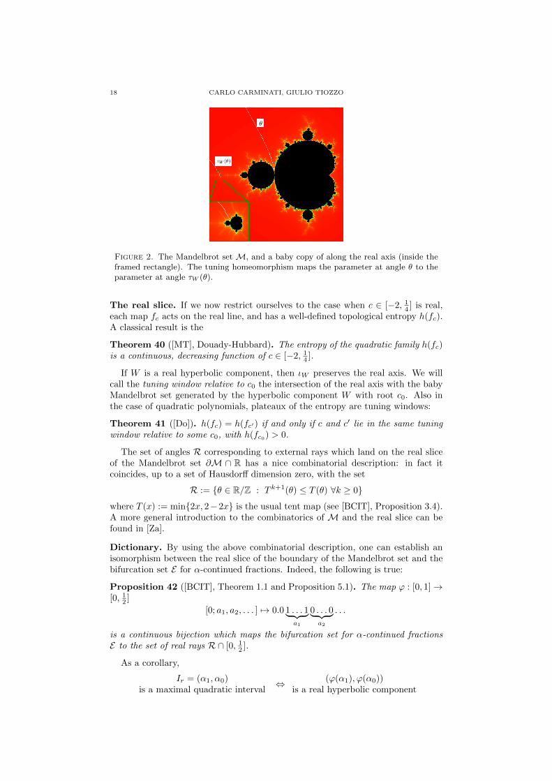
Figure 2. The Mandelbrot set M, and a baby copy of along the real axis (inside theframed rectangle). The tuning homeomorphism maps the parameter at angle θ to theparameter at angle τW (θ).

The real slice. If we now restrict ourselves to the case when c ∈ [−2, 14 ] is real,each map fc acts on the real line, and has a well-defined topological entropy h(fc).A classical result is the

Theorem 40 ([MT], Douady-Hubbard). The entropy of the quadratic family h(fc)is a continuous, decreasing function of c ∈ [−2, 14 ].

If W is a real hyperbolic component, then ιW preserves the real axis. We willcall the tuning window relative to c0 the intersection of the real axis with the babyMandelbrot set generated by the hyperbolic component W with root c0. Also inthe case of quadratic polynomials, plateaux of the entropy are tuning windows:

Theorem 41 ([Do]). h(fc) = h(fc′) if and only if c and c′ lie in the same tuningwindow relative to some c0, with h(fc0) > 0.

The set of angles R corresponding to external rays which land on the real sliceof the Mandelbrot set ∂M ∩ R has a nice combinatorial description: in fact itcoincides, up to a set of Hausdorff dimension zero, with the set

R := {θ ∈ R/Z : T k+1(θ) ≤ T (θ) ∀k ≥ 0}

where T (x) := min{2x, 2−2x} is the usual tent map (see [BCIT], Proposition 3.4).A more general introduction to the combinatorics of M and the real slice can befound in [Za].

Dictionary. By using the above combinatorial description, one can establish anisomorphism between the real slice of the boundary of the Mandelbrot set and thebifurcation set E for α-continued fractions. Indeed, the following is true:

Proposition 42 ([BCIT], Theorem 1.1 and Proposition 5.1). The map ϕ : [0, 1]→[0, 12 ]

[0; a1, a2, . . . ] 7→ 0.0 1 . . . 1︸︷︷︸a1

0 . . . 0︸︷︷︸a2

. . .

is a continuous bijection which maps the bifurcation set for α-continued fractionsE to the set of real rays R∩ [0, 12 ].

As a corollary,

Ir = (α1, α0)is a maximal quadratic interval

⇔ (ϕ(α1), ϕ(α0))is a real hyperbolic component


Let us now check that the definition of tuning operators given in section 4 andthe Douady-Hubbard tuning correspond to each other via the dictionary:

Proposition 43. Suppose W is a real hyperbolic component and let c ∈ ∂M∩ Rbe its root. Moreover, let η0 ∈ [0, 12 ] be the external angle of a ray which lands at c.Suppose η0 has binary expansion

η0 = 0.0 1 . . . 1︸︷︷︸b1

0 . . . 0︸︷︷︸b2

. . . 0 . . . 0︸︷︷︸bn−1

Then, for each x ∈ [0, 1],

τW (ϕ(x)) = ϕ(τr(x))

with r = [0; b1, . . . , bn].

Proof. Suppose x = [0; a1, a2, . . . ] so that τr(x) = [0;S1Sa1−10 S1S

a2−10 . . . ]. Then

by definition

ϕ(τr(x)) = 0.01b1 . . . 0bn−11(0b1 . . . 1bn

)a1−10b1 . . . 1bn−10

(1b1 . . . 0bn

)a2−1 · · · == 0.

(01b1 . . . 0bn−1

) (10b1 . . . 1bn−1

)a1 · · · = 0.Σ0Σa11 Σa20 Σa31 · · · = τW (θ)

where θ = 0.01a10a2 · · · = ϕ(x). �

Let us point out that thinking in terms of binary expansions often simplifies thecombinatorial picture: as an example, since the monotonicity of τW is straightfor-ward, the dictionary gives a simpler alternative proof of Lemma 13.

References

[BCIT] C. Bonanno, C. Carminati, S. Isola, G. Tiozzo, Dynamics of continued fractions andkneading sequences of unimodal maps, to appear in Discrete Contin. Dyn. Syst. (A), available

at arXiv:1012.2131 [math.DS].

[BDV] J Bourdon, B Daireaux, B Vallee, Dynamical analysis of α-Euclidean algorithms, J.Algorithms, 44 (2002), 1, 246–285.

[Ca] A. Cassa, Dinamiche caotiche e misure invarianti, Tesi di Laurea, University of Florence,

1995.[CMPT] C Carminati, S Marmi, A Profeti, G Tiozzo, The entropy of α-continued fractions:

numerical results, Nonlinearity 23 (2010) 2429-2456.[CT] C Carminati, G Tiozzo, A canonical thickening of Q and the entropy of α-continued

fractions, to appear in Ergodic Theory Dynam. Systems, available on CJO 2011

doi:10.1017/S0143385711000447.[CT2] C Carminati, G Tiozzo, The bifurcation locus for the set of bounded type numbers,

arXiv:1109.0516 [math.DS].

[Do] A Douady, Topological entropy of unimodal maps: monotonicity for quadratic polynomials,Real and complex dynamical systems (Hillerød, 1993), NATO Adv. Sci. Inst. Ser. C Math.

Phys. Sci., 464, 65–87, Kluwer Acad. Publ., Dordrecht, 1995.

[DH] A Douady, J H Hubbard, On the dynamics of polynomial-like mappings, Ann. Sci. Ecole

Norm. Sup. (4), 18 (1985), 2, 287–343.

[Fa] K Falconer, Fractal geometry: mathematical foundations and applications, Wiley, Chich-ester, 1990.

[He] D Hensley, A polynomial time algorithm for the Hausdorff dimension of continued fractionCantor sets, J. Number Theory, 58 (1996), 1, 9–45.

[IK] M Iosifescu, C Kraaikamp Metrical theory of continued fractions. Mathematics and its

Applications, 547. Kluwer Academic Publishers, Dordrecht, 2002.

[KSS] C. Kraaikamp, T. A. Schmidt, W. Steiner, Natural extensions and entropy of α-continued fractions, arXiv:1011.4283 [math.DS].

[LM] L Luzzi, S Marmi, On the entropy of Japanese continued fractions, Discrete Contin. Dyn.Syst. 20 (2008), 673–711.

[MCM] P Moussa, A Cassa, S Marmi, Continued fractions and Brjuno functions, Continued

fractions and geometric function theory (CONFUN) (Trondheim, 1997), J. Comput. Appl.Math. 105 (1999), 1-2, 403–415.

[MMY] S Marmi, P Moussa, J-C Yoccoz, The Brjuno functions and their regularity properties,

Comm. Math. Phys. 186 (1997), 2, 265–293.

http://arxiv.org/abs/1012.2131




[MT] J Milnor, W Thurston, On iterated maps of the interval, Dynamical systems (College

Park, MD, 1986–87), Lecture Notes in Math. 1342, 465–563, Springer, Berlin, 1988.

[Na] H Nakada, Metrical theory for a class of continued fraction transformations and theirnatural extensions, Tokyo J. Math. 4 (1981), 399–426.

[NN] H Nakada, R Natsui, The non-monotonicity of the entropy of α-continued fraction trans-formations, Nonlinearity 21 (2008), 1207–1225.

[Sc] F Schweiger, Ergodic theory of fibred systems and metric number theory, Oxford Science

Publications, The Clarendon Press Oxford University Press, New York, 1995.[Ti] G Tiozzo, The entropy of α-continued fractions: analytical results, arXiv:0912.2379

[math.DS].

[Za] S Zakeri, External rays and the real slice of the Mandelbrot set, Ergodic Theory Dynam.Systems 23 (2003), 2, 637–660.

(Carlo Carminati) Dipartimento di Matematica, Universita di Pisa, Largo Bruno Pon-

tecorvo 5, I-56127, ItalyE-mail address, Carlo Carminati: [email protected]

(Giulio Tiozzo) Department of Mathematics, Harvard University, One Oxford Street

Cambridge MA 02138 USAE-mail address, Giulio Tiozzo: [email protected]


Documents

Tuning and plateaux for the entropy of $\alpha$-continued fractions