Embed Size (px)
Citation preview
The entropy of α-continued fractions:
numerical results
Carlo Carminati, Stefano Marmi, Alessandro Profeti, Giulio Tiozzo
28 November, 2009
Abstract
We consider the one-parameter family of interval maps arising fromgeneralized continued fraction expansions known as α-continued fractions.For such maps, we perform a numerical study of the behaviour of metricentropy as a function of the parameter. The behaviour of entropy is knownto be quite regular for parameters for which a matching condition on theorbits of the endpoints holds. We give a detailed description of the setM where this condition is met: it consists of a countable union of openintervals, corresponding to different combinatorial data, which appear tobe arranged in a hierarchical structure. Our experimental data suggestthat the complement of M is a proper subset of the set of bounded-typenumbers, hence it has measure zero. Furthermore, we give evidence thatthe entropy on matching intervals is smooth; on the other hand, we canconstruct points outside of M on which it is not even locally monotone.
1 Introduction
Let α ∈ [0, 1]. We will study the one-parameter family of one-dimensional mapsof the interval
Tα : [α− 1, α]→ [α− 1, α]
Tα(x) =
{1|x| −
⌊1|x| + 1− α
⌋if x 6= 0
0 if x = 0
If we let xn,α = Tnα (x), an,α =⌊
1|xn−1,α| + 1− α
⌋, εn,α = Sign(xn−1,α), then
for every x ∈ [α− 1, α] we get the expansion
x =ε1,α
a1,α + ε2,αa2,α+ . . .
with ai,α ∈ N, εi,α ∈ {±1} which we call α-continued fraction. These sys-tems were introduced by Nakada ([11]) and are also known in the literature asJapanese continued fractions.
1
arX
iv:0
912.
2329
v1 [
mat
h.D
S] 1
1 D
ec 2
009
The algorithm, analogously to Gauss’ map in the classical case, providesrational approximations of real numbers. The convergents pn,α
qn,αare given by{
p−1,α = 1 p0,α = 0 pn+1,α = εn+1,αpn−1,α + an+1,αpn,αq−1,α = 0 q0,α = 1 qn+1,α = εn+1,αqn−1,α + an+1,αqn,α
It is known (see [9]) that for each α ∈ (0, 1] there exists a unique invariantmeasure µα(dx) = ρα(x)dx absolutely continuous w.r.t. Lebesgue measure.
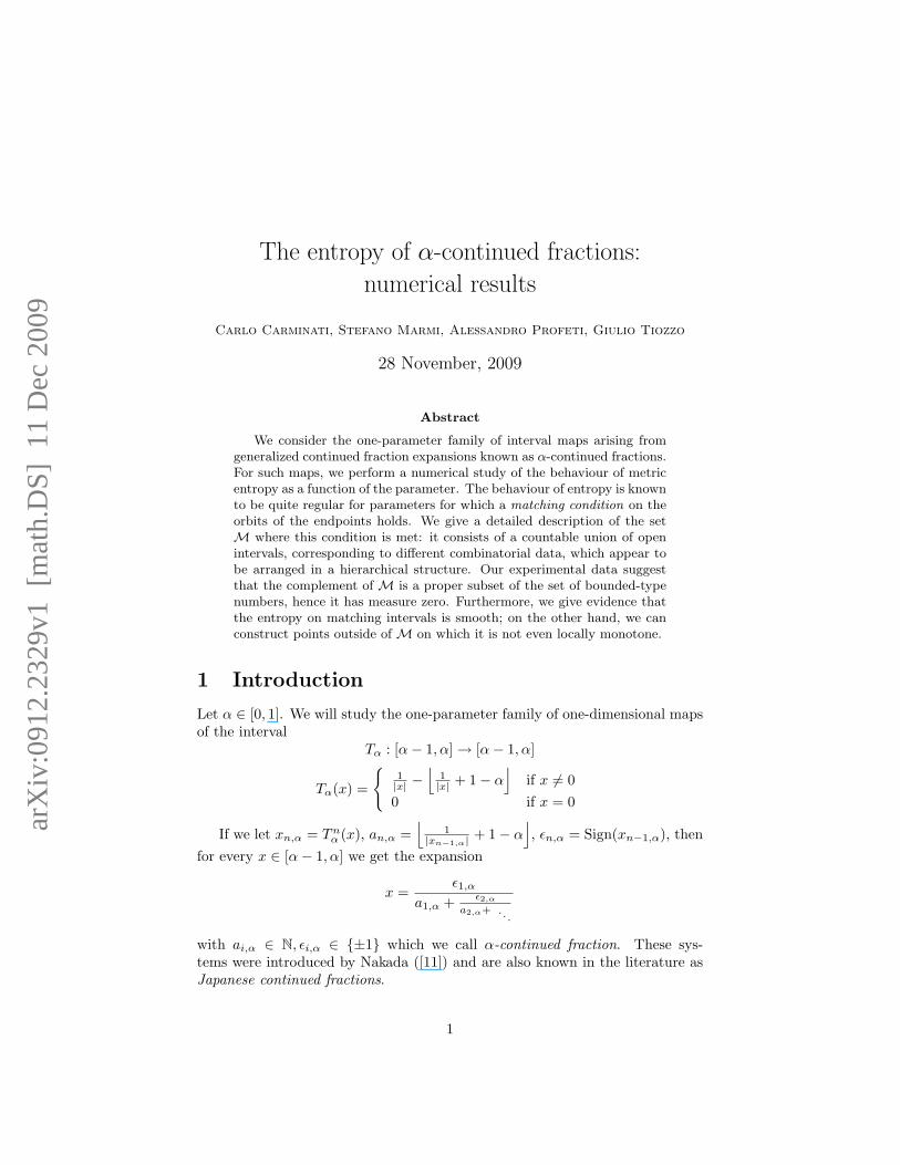
Figure 1: Graph of Tα
In this paper we will focus on the metric entropy of the Tα’s, which byRohlin’s formula ([13]) is given by
h(Tα) = −2∫ α
α−1
log |x|ρα(x)dx
Equivalently, entropy can be thought of as the average exponential growth rateof the denominators of convergents: for µα-a.e. x ∈ [α− 1, α],
h(Tα) = 2 limn→∞
1n
log qn,α(x)
The exact value of h(Tα) has been computed for α ≥ 12 by Nakada ([11])
and for√
2− 1 ≤ α ≤ 12 by Cassa, Marmi and Moussa ([10]).
In [9], Luzzi and Marmi computed numerically the entropy for α ≤√
2 − 1by approximating the integral in Rohlin’s formula with Birkhoff averages
h(α,N, x) = − 2N
N−1∑j=0
log |T jα(x)|
2
for a large number M of starting points x ∈ (α− 1, α) and then averaging overthe samples:
h(α,N,M) =1M
M∑k=1
h(α, n, xk)
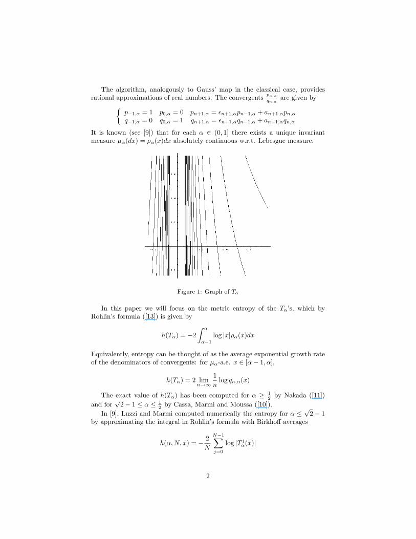
Their computations show a rich structure for the behaviour of the entropy asa function of α; it seems that the function α 7→ h(Tα) is piecewise regular andchanges monotonicity on different intervals of regularity.
These features have been confirmed by some results by Nakada and Natsui([12], thm. 2) which give a matching condition on the orbits of α and α− 1
T k1α (α) = T k2α (α− 1) for some k1, k2 ∈ N
which allows to find countable families of intervals where the entropy is in-creasing, decreasing or constant (see section 3). It is not difficult to check thatthe numerical data computed via Birkhoff theorem fit extremely well with thematching intervals of [12].
Figure 2: Numerical data vs. matching intervals
In this paper we will study the matching condition in great detail. First of all,we analyze the mechanism which produces it from a group-theoretical point ofview and find an algorithm to relate the α-continued fraction expansion of α andα− 1 when a matching occurs. This allows us to understand the combinatoricsbehind the matchings once and for all, without having to resort to specific matrixidentities. As an example, we will explicitly construct a family of matchingintervals which accumulate on a point different from 0. In fact we also havenumerical evidence that there exist positive values, such as [0, 3, 1], which arecluster point for intervals of all the three matching types: with k1 < k2, k1 = k2
and k1 > k2.
3
We then describe an algorithm to produce a huge quantity of matchingintervals, whose exact endpoints can be found computationally, and analyze thedata thus obtained. These data show matching intervals are organized in ahierarchical structure, and we will describe a recursive procedure which shouldproduce such structure.
Let now M be the union of all matching intervals. It has been conjectured([12], sect. 4, pg. 1213) thatM is an open, dense set of full Lebesgue measure.In fact, the correctness of our scheme would imply the following stronger
Conjecture 1.1. For any n, all elements of ( 1n+1 ,
1n ]\M have regular continued
fraction expansion bounded by n.
Since the set of numbers with bounded continued fraction expansion hasLebesgue measure zero, this clearly implies the previous conjecture.
We will then discuss some consequences of these matchings on the shapeof the entropy function, coming from a formula in [12]. This formula allowsus to recover the behaviour of entropy in a neighbourhood of points where amatching condition is present. First of all, we will use it to prove that entropyhas one-sided derivatives at every point belonging to some matching interval,and also to recover the exact value of h(Tα) for α ≥ 2/5. In general, though, toreconstruct the entropy one also has to know the invariant density at one point.
As an example, we shall examine the entropy on an interval J on which (byprevious experiments, see [9], sect. 3) it was thought to be linearly increasing:we numerically compute the invariant density for a single value of α ∈ J anduse it to predict the analytical form of the entropy on J , which in fact happensto be not linear. The data produced with this extrapolation method agree withhigh precision, and much better than any linear fit, with the values of h(Tα)computed via Birkhoff averages.
The paper is structured as follows: in section 2 we will discuss numericalsimulations of the entropy and provide some theoretical framework to justify theresults; in section 3 we shall analyze the mechanisms which produce the match-ing intervals and in section 4 we will numerically produce them and study theirhierarchical structure; in section 5 we will see how these matching conditionsaffect the entropy function.
Acknowledgements
This research was partially supported by the project “Dynamical Systems andApplications” of the Italian Ministry of University and Research1, and the Cen-tro di Ricerca Matematica “Ennio De Giorgi”.
1PRIN 2007B3RBEY.
4
2 Numerical computation of the entropy
Let us examine more closely the algorithm used in [9] to compute the entropy.A numerical problem in evaluating Birkhoff averages arises from the fact thatthe orbit of a point can fall very close to the origin: the computer will notdistinguish a very small value from zero. In this case we neglect this point, andcomplete the (pseudo)orbit restarting from a new random seed2. As a matterof fact this algorithm produces an approximate value of
hε(α) :=∫Iα
fε(x)dµα(x) with fε(x) :={
0 |x| ≤ ε−2 log |x| |x| > ε
where ε = 10−16; of course hε(α) is an excellent approximation of the entropyh(α), since the difference is of order ε log ε−1. To calculate hε(α) we use theBirkhoff sums
hε(α,N, x) :=1N
N−1∑j=0
fε(T jα(x))
and in [16] the fourth author proves that for large N the random variableh(ε,N, ·) is distributed around its mean hε(α) approximately with normal lawand standard deviation σε(α)/
√N where
σ2ε (α) := lim
n→+∞
∫Iα
(Snfε − n
∫fεdµα√
n
)2
dµα
which explains the aforementioned result by Luzzi and Marmi [9].One of our goals is to study the function α 7→ σ2
ε (α), in particular we askwhether it displays some regularity like continuity or semicontinuity. To thisaim we pushed the same scheme as in [9] to get higher precision:
1. We take a sample of values α chosen in a particular subinterval J ⊂ [0, 1];
2. For each value α we choose a random sample {x1, ..., xM} in Iα (the car-dinality M of this sample is usually 106 or 107);
3. For each xi ∈ Iα (i = 1, ...,M) we evaluate hε(α,N, xi) as described before(the number of iterates N will be 104);
4. Finally, we evaluate the (approximate) entropy and take record of standarddeviation as well:
hε(α,N,M) :=1M
M∑i=1
hε(α,N, xi)
σε(α) :=
√√√√ 1M
M∑i=1
[hε(α,N, xi)− hε(α,N,M)]2.
2Another choice is to throw away the whole orbit and restart; it seems there is not muchdifference on the final result
5
2.1 Central limit theorem
Let us restate more precisely the convergence result for Birkhoff sums proved in[16]. Let us denote by BV (Iα) the space of real-valued, µα-integrable, boundedvariation functions of the interval Iα. We will denote by Snf the Birkhoff sum
Snf =n−1∑j=0
f ◦ T jα
Lemma 2.1. Let α ∈ (0, 1] and f be an element of BV (Iα). Then the sequence
Mn =∫Iα
(Snf − n
∫fdµα√
n
)2
dµα
converges to a real nonnegative value, which will be denoted by σ2. Moreover,σ2 = 0 if and only if there exists u ∈ L2(µα) such that uρα ∈ BV (Iα) and
f −∫Iα
fdµα = u− u ◦ Tα (1)
The condition given by (1) is the same as in the proof of the central limittheorem for Gauss’ map, and it’s known as cohomological equation. The mainstatement of the theorem is the following:
Theorem 2.2. Let α ∈ (0, 1] and f be an element of BV (Iα) such that (1) hasno solutions. Then, for every v ∈ R we have
limn→∞
µα
(Snf − n
∫Ifdµα
σ√n
≤ v)
=1√2π
∫ v
−∞e−x
2/2dx
Since we know that the invariant density ρα is bounded from below by anonzero constant, we can show that
Proposition 2.3. For every real-valued nonconstant f ∈ BV (Iα), the equation(1) has no solutions. Hence, the central limit theorem holds.
Now, for every ε > 0 the function fε define in the previous section is ofbounded variation, hence the central limit theorem holds and the distributionof the approximate entropy hε(α,N, ·) approaches a Gaussian when N → ∞.As a corollary, for the standard deviation of Birkhoff averages
Std[Snfεn
]= E
[(Snfεn−∫Iα
fεdµα
)2]1/2
=σ√n
+ o
(1√n
)
2.2 Speed of convergence
In terms of numerical simulations it is of primary importance to estimate thedifference between the sum computed at the nth step and the asymptotic value:a semi-explicit bound is given by the following
6
Theorem 2.4. For every nonconstant real-valued f ∈ BV (Iα), there existsC > 0 such that
supv∈R
[µα
(Snf − n
∫Iαfdµα
σ√n
≤ v
)− 1√
2π
∫ v
−∞e−
x22 dx
]≤ C√
n
Proof. It follows from a Berry-Esseen type of inequality. For details see ([1],th.8.1).
2.3 Dependence of standard deviation on α
Given these convergence results for the entropy, it is natural to ask how thestandard deviation varies with α. In this case not a single exact value of σε(α)is known; by using the fact that natural extensions of Tα are conjugate ([7],[12]), it is straightforward to prove the
Lemma 2.5. The map α 7→ σ(α) is constant for α ∈ [√
2− 1,√
5−12 ].
Proof. See appendix.
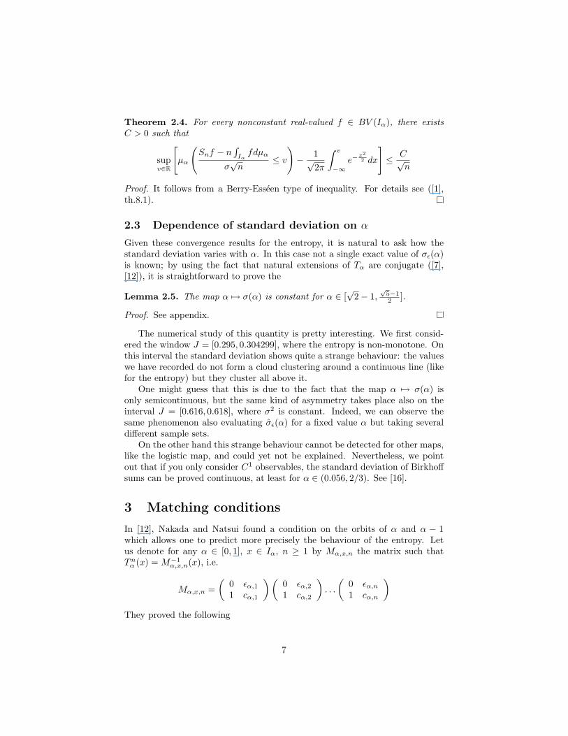
The numerical study of this quantity is pretty interesting. We first consid-ered the window J = [0.295, 0.304299], where the entropy is non-monotone. Onthis interval the standard deviation shows quite a strange behaviour: the valueswe have recorded do not form a cloud clustering around a continuous line (likefor the entropy) but they cluster all above it.
One might guess that this is due to the fact that the map α 7→ σ(α) isonly semicontinuous, but the same kind of asymmetry takes place also on theinterval J = [0.616, 0.618], where σ2 is constant. Indeed, we can observe thesame phenomenon also evaluating σε(α) for a fixed value α but taking severaldifferent sample sets.
On the other hand this strange behaviour cannot be detected for other maps,like the logistic map, and could yet not be explained. Nevertheless, we pointout that if you only consider C1 observables, the standard deviation of Birkhoffsums can be proved continuous, at least for α ∈ (0.056, 2/3). See [16].
3 Matching conditions
In [12], Nakada and Natsui found a condition on the orbits of α and α − 1which allows one to predict more precisely the behaviour of the entropy. Letus denote for any α ∈ [0, 1], x ∈ Iα, n ≥ 1 by Mα,x,n the matrix such thatTnα (x) = M−1
α,x,n(x), i.e.
Mα,x,n =(
0 εα,11 cα,1
)(0 εα,21 cα,2
). . .
(0 εα,n1 cα,n
)They proved the following
7
Figure 3: Variance on the interval J = [0.295, 0.304299].
Theorem 3.1. ([12], thm. 2) Let us suppose that there exist positive integersk1 and k2 such that
(I) {Tnα (α) : 0 ≤ n < k1} ∩ {Tmα (α− 1) : 0 ≤ m < k2} = ∅
(II) Mα,α,k1 =(
1 10 1
)Mα,α−1,k2 [ =⇒ T k1α (α) = T k2α (α− 1) ]
(III) T k1α (α)[
= T k2α (α− 1)]/∈ {α, α− 1}
Then there exists η > 0 such that, on (α− η, α+ η), h(Tα) is :
(i) strictly increasing if k1 < k2
(ii) constant if k1 = k2
(iii) strictly decreasing if k1 > k2
It turns out that conditions (I)-(II)-(III) define a collection of open intervals(called matching intervals); they also proved that each of the cases (i), (ii) and(iii) takes place at least on one infinite family of disjoint matching intervals clus-tering at the origin, thus proving the non-monotonicity of the entropy function.Moreover, they conjectured that the union of all matching intervals is a dense,open subset of [0, 1] with full Lebesgue measure.
8
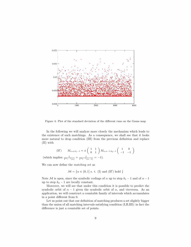
Figure 4: Plot of the standard deviation of the different runs on the Gauss map
In the following we will analyze more closely the mechanism which leads tothe existence of such matchings. As a consequence, we shall see that it looksmore natural to drop condition (III) from the previous definition and replace(II) with
(II′) Mα,α,k1−1 = ±„
1 10 1
«Mα,α−1,k2−1
„1 0−1 −1
«(which implies 1
Tk1−1(α)+ 1
Tk2−1(α−1)= −1).
We can now define the matching set as
M = {α ∈ (0, 1] s. t. (I) and (II′) hold }
NoteM is open, since the symbolic codings of α up to step k1 − 1 and of α− 1up to step k2 − 1 are locally constant.
Moreover, we will see that under this condition it is possible to predict thesymbolic orbit of α − 1 given the symbolic orbit of α, and viceversa. As anapplication, we will construct a countable family of intervals which accumulatesin a point different from 0.
Let us point out that our definition of matching produces a set slightly biggerthan the union of all matching intervals satisfying condition (I,II,III): in fact thedifference is just a countable set of points.
9
3.1 Structure of PGL(2, Z)
Let us define PGL(2,Z) := GL(2,Z)/{±I}, PSL(2,Z) := SL(2,Z)/{±I}. Wehave an exact sequence
1→ PSL(2,Z)→ PGL(2,Z)→ {±1} → 1
where the first arrow is the inclusion and the second the determinant; moreover,if we consider the group
C ={(±1 00 ±1
)}∼=
Z2Z× Z
2Z
and let C = C/{±I}, then
C ∩ PSL(2,Z) = {e}
therefore we have the semidirect product decomposition
PGL(2,Z) = PSL(2,Z) o C
Now, it is well known that PSL(2,Z) is the free product
PSL(2,Z) =< S > ? < U >
where
S =(
0 −11 0
)U =
(0 −11 1
)are such that S2 = I, U3 = I. Geometrically, S represents the function {z →− 1z}, and if we denote by T the element corresponding to the translation {z →
z + 1}, we have U = ST .
The matrix V =(−1 00 1
)projects to a generator of C and it satisfies
V 2 = I, V SV −1 = V SV = S and V TV −1 = T−1 in PGL(2,Z) so we get thepresentation
PGL(2,Z) = {S, T, V | S2 = I, (ST )3 = I, V 2 = I, V SV −1 = S, V TV −1 = T−1}
3.2 Encoding of matchings
Every step of the algorithm generating α-continued fractions consists of an op-eration of the type:
z 7→ ε
z− c ε ∈ {±1}, c ∈ N
which corresponds to the matrix T−cSV e(ε) with
e(ε) ={
0 if ε = −11 if ε = 1
10
so if x belongs to the cylinder ((c1, ε1), . . . , (ck, εk)) we can express
T kα(x) = T−ckSV e(εk) . . . T−c1SV e(ε1)(x)
Now, suppose we have a matching T k1α (α) = T k2α (α − 1) and let α be-long to the cylinder ((a1, ε1), . . . , (ak1 , εk1)) and α − 1 belong to the cylinder((b1, η1), . . . , (bk2 , ηk2)). One can rewrite the matching condition as
T−ak1SV e(εk1 ) . . . T−a1SV e(ε1)(α) = T−bk2SV e(ηk2 ) . . . T−b1SV e(η1)T−1(α)
hence it is sufficient to have an equality of the two Mobius transformations
T−ak1SV e(εk1 ) . . . T−a1SV e(ε1) = T−bk2SV e(ηk2 ) . . . T−b1SV e(η1)T−1
We call such a matching an algebraic matching. Now, numerical evidence showsthat, if a matching occurs, then
ε1 = +1εi = −1 for 2 ≤ i ≤ k1 − 1ηi = −1 for 1 ≤ i ≤ k2 − 1
If we make this assumption we can rewrite the matching condition as
V e(εk1 )+1T ak1 (−1)e(εk1
)
ST ak1−1S · · ·T a1S =
= V e(ηk2 )T bk2 (−1)[e(ηk2
)+1]
ST−bk2−1S · · ·T−b1ST−1
which implies e(εk1) = e(ηk2) + 1, i.e. εk1ηk2 = −1. If for instance e(εk1) = 1and e(ηk2) = 0, by substituting T = SU one has
(U2S)ak1U(SU)ak1−1−2SU2 . . . SU2(SU)a1−2SUS =
= (U2S)bk2−1US(U2S)bk2−1−2US . . . US(U2S)b1−2US
Since every element of PSL(2,Z) can be written as a product of S and U ina unique way, one can get a relation between the ar and br. Notice that, sincewe are interested in α ≤
√2− 1, ai ≥ 2 and bi ≥ 2 for every i, hence there is no
cancellation in the equation above. By counting the number of (U2S) blocks atthe beginning of the word, one has ak1 = bk2 − 1, and by semplifying,
(SU)ak1−1−2SU2 . . . SU2(SU)a1−2SUS == S(U2S)bk2−1−2US . . . US(U2S)b1−2US
(2)
If one has e(εk1) = 0 and e(ηk2) = 1 instead, the matching condition is
(SU)ak1−1SU2(SU)ak1−1−2SU2 . . . SU2(SU)a1−2SUS =
(SU)bk2SU2S(U2S)bk2−1−2US . . . US(U2S)b1−2US
which implies bk2 = ak1 − 1, and simplifying still yields equation (2).
11
Let us remark that (2) is equivalent to
T−1ST−ak1−1S . . . T−a1SV = V ST−bk2−1S . . . T−b1ST−1
which is precisely condition (II′): by evaluating both sides on α
1T k1−1(α)
+1
T k2−1(α− 1)= −1
Moreover, from (2) one has that to every ar bigger than 2 it correspondsexactly a sequence of bi = 2 of length precisely ar − 2, and viceversa. Moreformally, one can give the following algorithm to produce the coding of theorbit of α − 1 up to step k2 − 1 given the coding of the orbit of α up to stepk1− 1 (under the hypothesis that an algebraic matching occurs, and at least k1
is known).
1. Write down the coding of α from step 1 to k1−1, separated by a symbol ?
a1 ? a2 ? · · · ? ak1−1
2. Subtract 2 from every ar; if ar = 2, then leave the space empty instead ofwriting 0.
a1 − 2 ? a2 − 2 ? · · · ? ak1−1 − 2
3. Replace stars with numbers and viceversa (replace the number n with nconsecutive stars, and write the number n in place of n stars in a row)
4. Add 2 to every number you find and remove the stars: you’ll get thesequence (b1, . . . , bk2−1).
Example. Let us suppose there is a matching with k1 = n+ 3 and α has initialcoding ((3,+), (4,−)n, (2,−)). The steps of the algorithm are:
Step 13 ? 4 ? 4 ? · · · ? 4?︸ ︷︷ ︸
n times
2
Step 21 ? 2 ? 2 ? · · · ? 2?︸ ︷︷ ︸
n times
Step 3?1 ? ? 1 ? ?1 . . . 1 ? ?1︸ ︷︷ ︸
n times
Step 42 3 2 3 . . . 2 3︸ ︷︷ ︸
n times
so the coding of α− 1 is ((2,−)(3,−))n+1, and k2 = 2n+ 3.
12
3.3 Construction of matchings
Let us now use this knowledge to construct explicitly an infinite family of match-ing intervals which accumulates on a non-zero value of α. For every n, let us con-sider the values of α such that α belongs to the cylinder ((3,+), (4,−)n, (2,−))with the respect to Tα. Let us compute the endpoints of such a cylinder.
• The right endpoint is defined by(−4 −11 0
)n( −3 11 0
)(α) = α− 1
i.e. (1 10 1
)(−4 −11 0
)n( −3 11 0
)(α) = α
• The left endpoint is defined by(−4 −11 0
)n( −3 11 0
)(α) = − 1
α+ 2
i.e. (−2 −11 0
)(−4 −11 0
)n( −3 11 0
)(α) = α
By diagonalizing the matrices and computing the powers one can computethese value explicitly. In particular,
α1min =
√3− 12
+40√
3− 6913
(2 +√
3)−2n +O((2 +√
3)−4n)
α1max =
√3− 12
+10√
3− 1213
(2 +√
3)−2n +O((2 +√
3)−4n)
The αs such that α−1 belongs to the cylinder ((2,−), (3,−))n+1 are definedby the equations[(
−3 −11 0
)(−2 −11 0
)]n+1
(α− 1) = α− 1
for the left endpoint and[(−3 −11 0
)(−2 −11 0
)]n+1
(α− 1) = α
for the right endpoint, so the left endpoint corresponds to the periodic pointsuch that [(
−3 −11 0
)(−2 −11 0
)](α− 1) = α− 1
i.e.
α2min =
√3− 12
13
and
α2max =
√3− 12
+33− 19
√3
2(2 +
√3)−2n +O((2 +
√3)−4n)
By comparing the first order terms one gets asymptotically
α2min < α1
min < α2max < α1
max
hence the two intervals intersect for infinitely many n, producing infinitely manymatching intervals which accumulate at the point α0 =
√3−12 . The length of
such intervals is
α2max − α1
min =567− 327
√3
26(2 +
√3)−2n +O((2 +
√3)−4n)
4 Numerical production of matchings
In this section we will describe an algorithm to produce a lot of matching in-tervals (i.e. find out their endpoints exactly), as well as the results we obtainedthrough its implementation. Our first attempt to find matching intervals usedthe following scheme:
1. We generate a random seed of values αi belonging to [0, 1] (or some otherinterval of interest). When a high precision is needed (we manage todetect intervals of size 10−60) the random seed is composed by algebraicnumbers, in order to allow symbolic (i.e. non floating-point) computation.
2. We find numerically candidates for the values of k1 and k2 (if any) simplyby computing the orbits of α and of α−1 up to some finite number of steps,and numerically checking if T k1α (α) = T k2α (α− 1) holds approximately forsome k1 and k2 smaller than some bound.
3. Given any triplet (α, k1, k2) determined as above, we compute the symbolicorbit of α up to step k1 − 1 and the orbit of α− 1 up to step k2 − 1.
4. We check that the two Mobius transformations associated to these sym-bolic orbits satisfy condition (II′):
Mα,α,k1−1 = ±(
1 10 1
)Mα,α−1,k2−1
(1 0−1 −1
)5. We solve the system of quadratic equations which correspond to imposing
that α and α−1 have the same symbolic orbit as α and α−1, respectively.
Let us remark that this is the heaviest step of the whole procedure sincewe must solve k1 + k2 − 2 quadratic inequalities; for this reason the valuek = k1 + k2 may be thought of as a measure of the computational cost ofthe matching interval and will be referred to as order of matching.
14
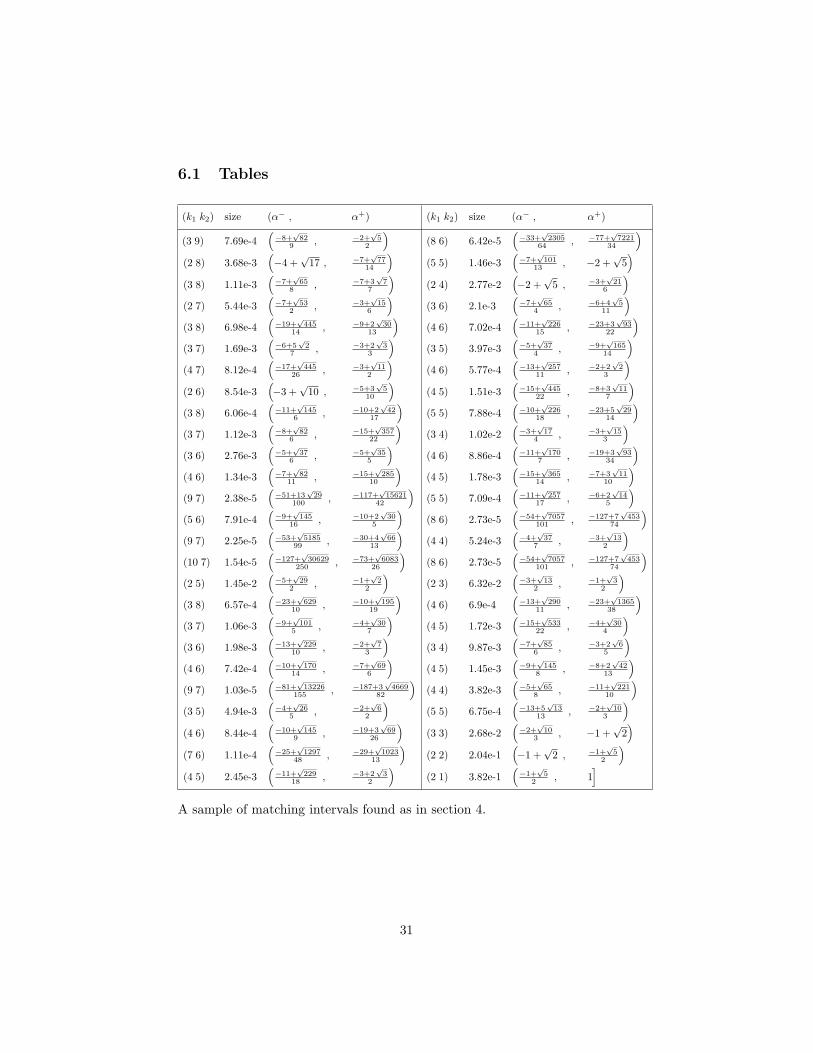
Following this scheme, we detected more than 107 matching intervals, whoseendpoints are quadratic surds; their union still leaves many gaps, each of whichsmaller than 6.6 · 10−6. A table with a sample of such data is contained in theappendix. 3
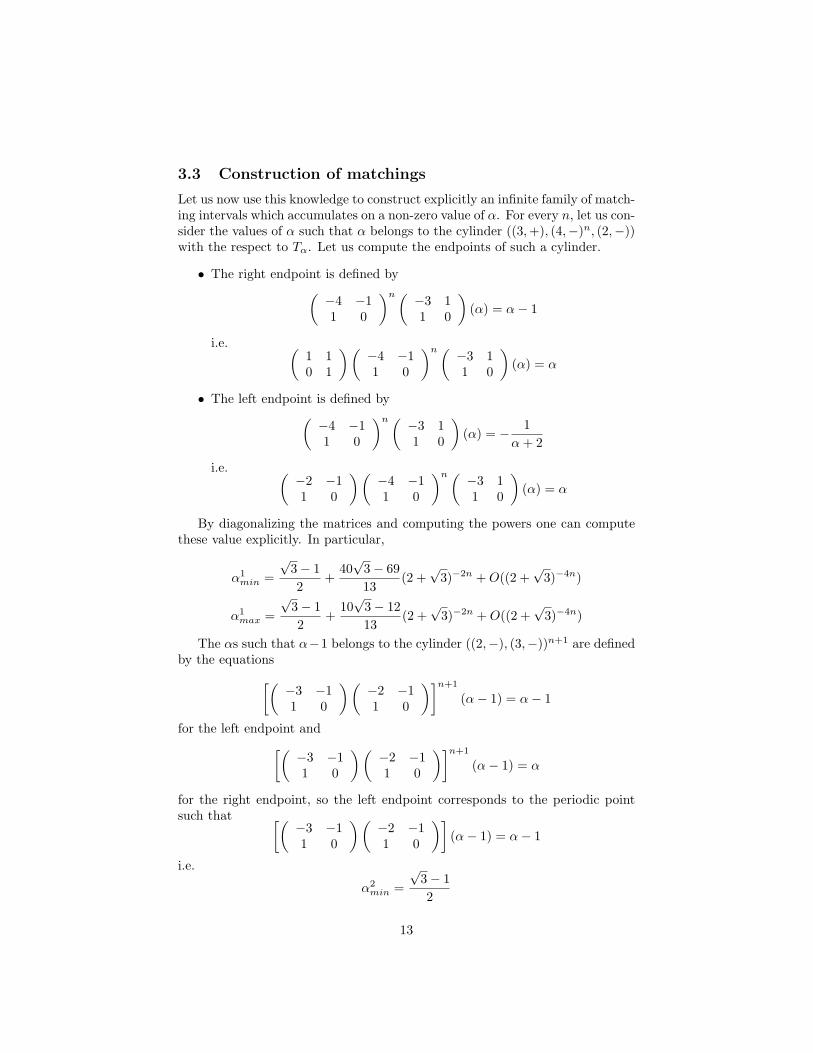
In order to detect some patterns in the data, let us plot the size of theseintervals (figure 5). For each matching interval ]α−, α+[, we drew the point ofcoordinates (α−, α+ − α−).
Figure 5: Size of matchings
It seems there is some self-similar pattern: in order to understand betterits structure it is useful to identify some “borderline” families of points. Themost evident family is the one that appears as the higher line of points inthe above figure (which we have highlighted in green): these points correspondto matching intervals which contain the values 1/n, and their endpoints areα−(n) = 1
2 [√n2 + 4 − n], α+(n) = 1
2n−2 [√n2 + 2n− 3 − n + 1]; this is the
family In already exhibited in [12]. Since α−(n) = 1/n − 1/n3 + o(1/n3) andα+(n) = 1/n + 1/n3 + o(1/n3), for n � 1 the points (α−(n), α+(n) − α−(n))are very close to ( 1
n ,1n3 ). This suggests that this family will “straighten” if we
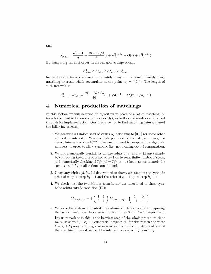
replot our data in log-log scale. This is indeed the case, and in fact it seemsthat there are also other families which get perfectly aligned along parallel linesof slope 3 (see figure 6).
If we consider the ordinary continued fraction expansion of the elements ofthese families we realize that they obey to some very simple empirical4 rules:
(i) the endpoints of any matching interval have a purely periodic continuedfraction expansion of the type [0, a1, a2, ..., am, 1] and [0, a1, a2, ..., am + 1];
3A more efficient algorithm, which avoids random sampling, will be discussed in subsec-tion 4.1.
4Unfortunately we are still not able to prove all these rules.
15
Figure 6: Same picture, in log-log scale.
this implies that the rational number corresponding to [0, a1, a2, ..., am+1]is a common convergent of both endpoints and is the rational with smallestdenominator which falls inside the matching interval;
(ii) any endpoint [0, a1, a2, ..., am] of a matching interval belongs to a family{[0, a, a2, ..., am] : a ≥ max2≤i≤m ai}; in particular this family has amember in each cylinder Bn := {α : 1/(n+ 1) < α < 1/n} for n ≥ a, sothat each family will cluster at the origin.
(ii’) other families can be detected in terms of the continued fraction expansion:for instance on each cylinder Bn (n ≥ 3) the largest matching interval onwhich h is decreasing has endpoints with expansion [0, n, 2, 1, n− 1, 1] and[0, n, 2, 1, n]
(iii) matching intervals seem to be organized in a binary tree structure, whichis related to the Stern-Brocot tree5: one can thus design a bisection al-gorithm to fill in the gaps between intervals, and what it’s left over is aclosed, nowhere dense set. This and the following points will be analyzedextensively in subsection 4.1;
(iv) if α ∈ Bn is the endpoint of some matching interval then α = [0; a1, a2, ..., am]with ai ≤ n ∀i ∈ {1, ...,m}; this would imply that the values α ∈ Bn whichdo not belong to any matching interval must be bounded-type numberswith partial quotients bounded above by n;
(v) it is possible to compute the exponent (k1, k2) of a matching from thecontinued fraction expansion of any one of its endpoints.
5Sometimes also known as Farey tree. See [3].
16
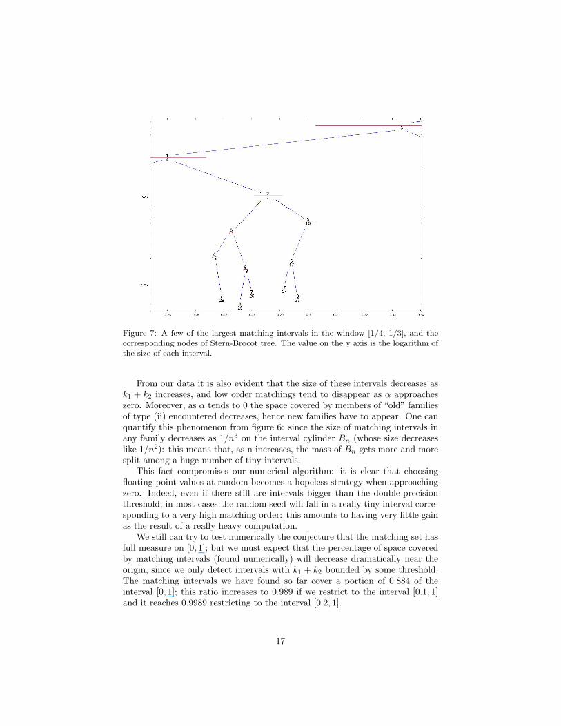
Figure 7: A few of the largest matching intervals in the window [1/4, 1/3], and thecorresponding nodes of Stern-Brocot tree. The value on the y axis is the logarithm ofthe size of each interval.
From our data it is also evident that the size of these intervals decreases ask1 + k2 increases, and low order matchings tend to disappear as α approacheszero. Moreover, as α tends to 0 the space covered by members of “old” familiesof type (ii) encountered decreases, hence new families have to appear. One canquantify this phenomenon from figure 6: since the size of matching intervals inany family decreases as 1/n3 on the interval cylinder Bn (whose size decreaseslike 1/n2): this means that, as n increases, the mass of Bn gets more and moresplit among a huge number of tiny intervals.
This fact compromises our numerical algorithm: it is clear that choosingfloating point values at random becomes a hopeless strategy when approachingzero. Indeed, even if there still are intervals bigger than the double-precisionthreshold, in most cases the random seed will fall in a really tiny interval corre-sponding to a very high matching order: this amounts to having very little gainas the result of a really heavy computation.
We still can try to test numerically the conjecture that the matching set hasfull measure on [0, 1]; but we must expect that the percentage of space coveredby matching intervals (found numerically) will decrease dramatically near theorigin, since we only detect intervals with k1 + k2 bounded by some threshold.The matching intervals we have found so far cover a portion of 0.884 of theinterval [0, 1]; this ratio increases to 0.989 if we restrict to the interval [0.1, 1]and it reaches 0.9989 restricting to the interval [0.2, 1].
17
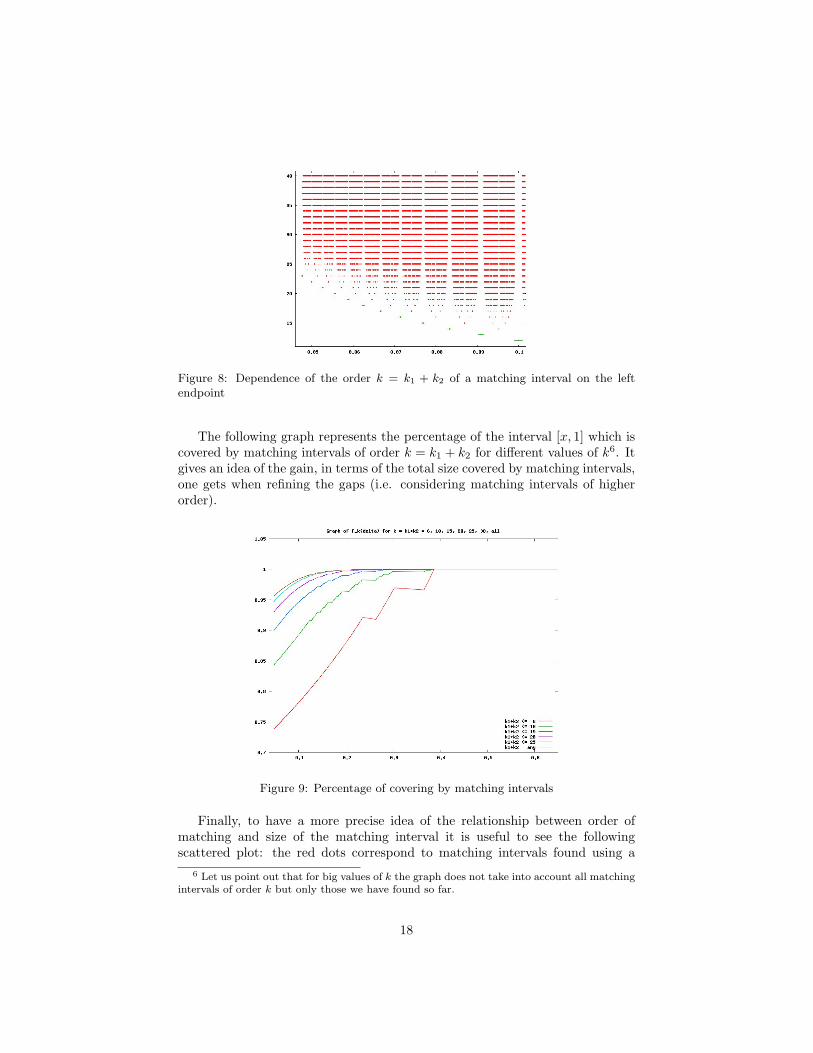
Figure 8: Dependence of the order k = k1 + k2 of a matching interval on the leftendpoint
The following graph represents the percentage of the interval [x, 1] which iscovered by matching intervals of order k = k1 + k2 for different values of k6. Itgives an idea of the gain, in terms of the total size covered by matching intervals,one gets when refining the gaps (i.e. considering matching intervals of higherorder).
Figure 9: Percentage of covering by matching intervals
Finally, to have a more precise idea of the relationship between order ofmatching and size of the matching interval it is useful to see the followingscattered plot: the red dots correspond to matching intervals found using a
6 Let us point out that for big values of k the graph does not take into account all matchingintervals of order k but only those we have found so far.
18
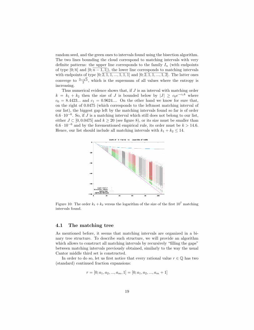
random seed, and the green ones to intervals found using the bisection algorithm.The two lines bounding the cloud correspond to matching intervals with verydefinite patterns: the upper line corresponds to the family In (with endpointsof type [0;n] and [0;n− 1, 1]), the lower line corresponds to matching intervalswith endpoints of type [0; 2, 1, 1, ..., 1, 1, 1] and [0; 2, 1, 1, ..., 1, 2]. The latter onesconverge to 3−
√5
2 , which is the supremum of all values where the entropy isincreasing.
Thus numerical evidence shows that, if J is an interval with matching orderk = k1 + k2 then the size of J is bounded below by |J | ≥ c0e
−c1k wherec0 = 8.4423... and c1 = 0.9624.... On the other hand we know for sure that,on the right of 0.0475 (which corresponds to the leftmost matching interval ofour list), the biggest gap left by the matching intervals found so far is of order6.6 · 10−6. So, if J is a matching interval which still does not belong to our list,either J ⊂ [0, 0.0475] and k ≥ 20 (see figure 8), or its size must be smaller than6.6 · 10−6 and by the forementioned empirical rule, its order must be k > 14.6.Hence, our list should include all matching intervals with k1 + k2 ≤ 14.
Figure 10: The order k1 + k2 versus the logarithm of the size of the first 107 matchingintervals found.
4.1 The matching tree
As mentioned before, it seems that matching intervals are organized in a bi-nary tree structure. To describe such structure, we will provide an algorithmwhich allows to construct all matching intervals by recursively “filling the gaps”between matching intervals previously obtained, similarly to the way the usualCantor middle third set is constructed.
In order to do so, let us first notice that every rational value r ∈ Q has two(standard) continued fraction expansions:
r = [0; a1, a2, ..., am, 1] = [0; a1, a2, ..., am + 1]
19
One can associate to r the interval whose endpoints are the two quadratic surdswith continued fraction obtained by endless repetition of the two expansions ofr:
Definition 4.1. Given r ∈ Q with continued fraction expansion as above, wedefine Ir to be the interval with endpoints
[0; a1, a2, ..., am, 1] and [0; a1, a2, ..., am + 1]
(in any order). The strings S1 := {a1, . . . , am, 1} and S2 := {a1, . . . , am + 1}will be said to be conjugate and we will write S2 = (S1)′.
Notice that r ∈ Ir. It looks like all matching intervals are of type Ir for somerational r. On the other hand,
Definition 4.2. Given an open interval I ⊇ [0, 1] one can define the pseudocen-ter of I as the rational number r ∈ I ∩Q which has the minimum denominatoramong all rational numbers contained in I.
It is straightforward to prove that the pseudocenter of an interval is unique, andthe pseudocenter of Ir is r itself.
We are now ready to describe the algorithm:
1. The rightmost matching interval is [√
5−12 , 1]; its complement is the gap
J = [0,√
5−12 ].
2. Suppose we are given a finite set of intervals, called gaps of level n, sothat their complement is a union of matching intervals. Given each gapJ = [α−, α+], we determine its pseudocenter r. Let α± = [0;S, a±, S±]be the continued fraction expansion of α±, where S is the finite stringcontaining the first common partial quotients, a+ 6= a− the first partialquotient on which the two values differ, and S± the rest of the expansion ofα±, respectively. The pseudocenter of [α−, α+] will be the rational numberr with expansions [0;S, a, 1] = p/q = [0;S, a+ 1] where a := min(a+, a−).
3. We remove from the gap J the matching interval Ir corresponding to thepseudocenter r: in this way the complement of Ir in J will consist of twointervals J1 and J2, which we will add to the list of gaps of level n+ 1. Itmight occur that one of these new intervals consists of only one point, i.e.two matching intervals are adjacent.
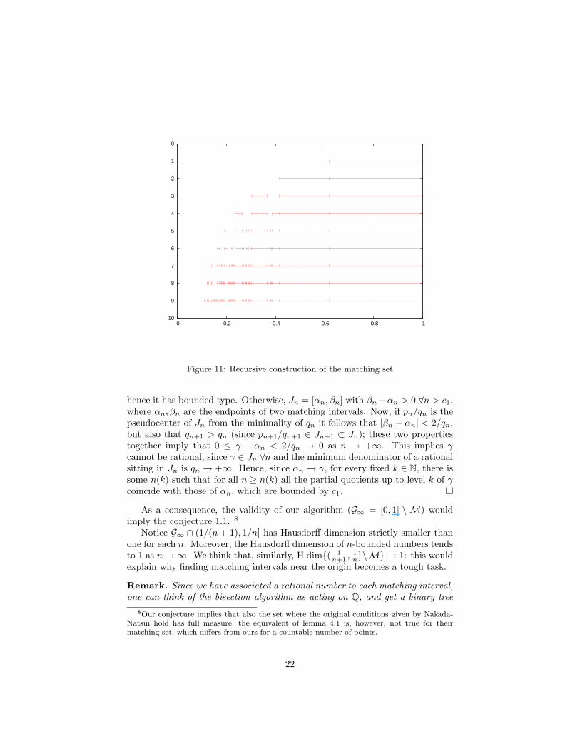
By iterating this procedure, after n steps we will get a finite set Gn of gaps,and clearly
⋃J∈Gn+1
J ⊆⋃J∈Gn J . We conjecture all intervals obtained by
taking pseudocenters of gaps are matching intervals, and that the set on whichmatching fails is the intersection
G∞ :=⋂n∈N
⋃J∈Gn
J,
20
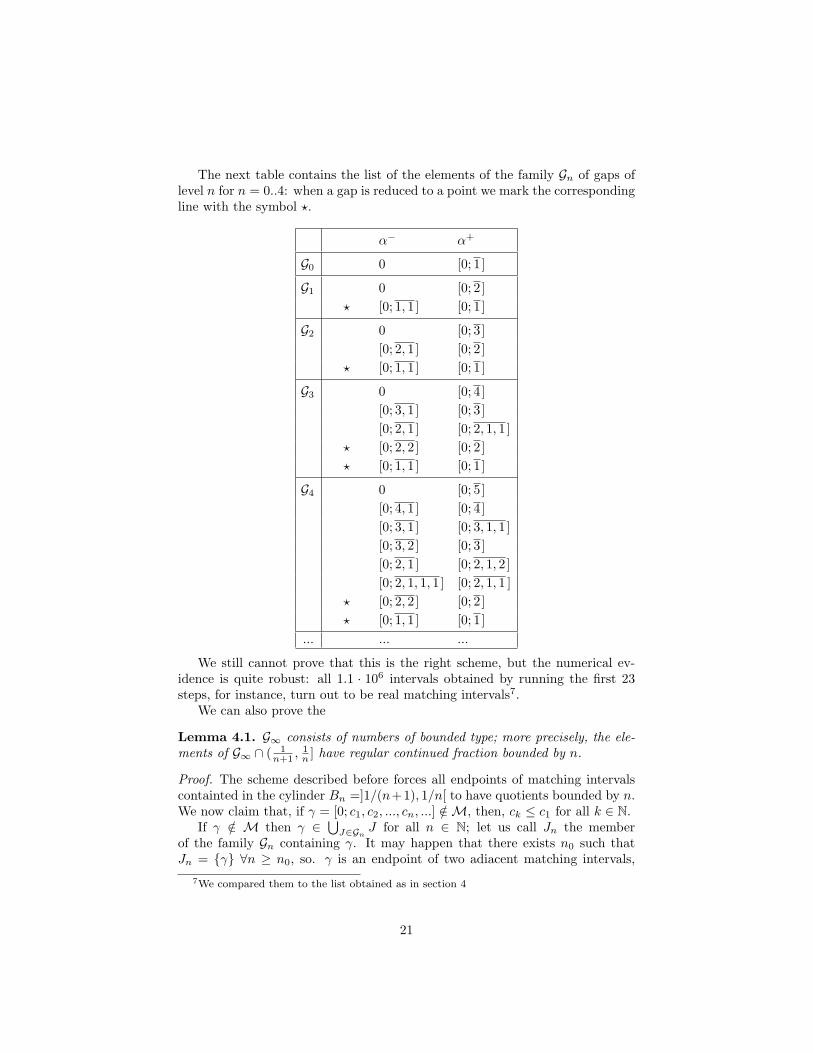
The next table contains the list of the elements of the family Gn of gaps oflevel n for n = 0..4: when a gap is reduced to a point we mark the correspondingline with the symbol ?.
α− α+
G0 0 [0; 1]
G1 0 [0; 2]? [0; 1, 1] [0; 1]
G2 0 [0; 3][0; 2, 1] [0; 2]
? [0; 1, 1] [0; 1]
G3 0 [0; 4][0; 3, 1] [0; 3][0; 2, 1] [0; 2, 1, 1]
? [0; 2, 2] [0; 2]? [0; 1, 1] [0; 1]
G4 0 [0; 5][0; 4, 1] [0; 4][0; 3, 1] [0; 3, 1, 1][0; 3, 2] [0; 3][0; 2, 1] [0; 2, 1, 2][0; 2, 1, 1, 1] [0; 2, 1, 1 ]
? [0; 2, 2] [0; 2]? [0; 1, 1] [0; 1]
... ... ...
We still cannot prove that this is the right scheme, but the numerical ev-idence is quite robust: all 1.1 · 106 intervals obtained by running the first 23steps, for instance, turn out to be real matching intervals7.
We can also prove the
Lemma 4.1. G∞ consists of numbers of bounded type; more precisely, the ele-ments of G∞ ∩ ( 1
n+1 ,1n ] have regular continued fraction bounded by n.
Proof. The scheme described before forces all endpoints of matching intervalscontainted in the cylinder Bn =]1/(n+1), 1/n[ to have quotients bounded by n.We now claim that, if γ = [0; c1, c2, ..., cn, ...] /∈M, then, ck ≤ c1 for all k ∈ N.
If γ /∈ M then γ ∈⋃J∈Gn J for all n ∈ N; let us call Jn the member
of the family Gn containing γ. It may happen that there exists n0 such thatJn = {γ} ∀n ≥ n0, so. γ is an endpoint of two adiacent matching intervals,
7We compared them to the list obtained as in section 4
21
0
1
2
3
4
5
6
7
8
9
10 0 0.2 0.4 0.6 0.8 1
Figure 11: Recursive construction of the matching set
hence it has bounded type. Otherwise, Jn = [αn, βn] with βn−αn > 0 ∀n > c1,where αn, βn are the endpoints of two matching intervals. Now, if pn/qn is thepseudocenter of Jn from the minimality of qn it follows that |βn − αn| < 2/qn,but also that qn+1 > qn (since pn+1/qn+1 ∈ Jn+1 ⊂ Jn); these two propertiestogether imply that 0 ≤ γ − αn < 2/qn → 0 as n → +∞. This implies γcannot be rational, since γ ∈ Jn ∀n and the minimum denominator of a rationalsitting in Jn is qn → +∞. Hence, since αn → γ, for every fixed k ∈ N, there issome n(k) such that for all n ≥ n(k) all the partial quotients up to level k of γcoincide with those of αn, which are bounded by c1.
As a consequence, the validity of our algorithm (G∞ = [0, 1] \ M) wouldimply the conjecture 1.1. 8
Notice G∞ ∩ (1/(n + 1), 1/n] has Hausdorff dimension strictly smaller thanone for each n. Moreover, the Hausdorff dimension of n-bounded numbers tendsto 1 as n→∞. We think that, similarly, H.dim{( 1
n+1 ,1n ]\M} → 1: this would
explain why finding matching intervals near the origin becomes a tough task.
Remark. Since we have associated a rational number to each matching interval,one can think of the bisection algorithm as acting on Q, and get a binary tree
8Our conjecture implies that also the set where the original conditions given by Nakada-Natsui hold has full measure; the equivalent of lemma 4.1 is, however, not true for theirmatching set, which differs from ours for a countable number of points.
22
whose nodes are rationals: this object is related to the well-known Stern-Brocottree. (For an introduction to it, see [3]).
Given that all matching intervals correspond to some rational number, onecan ask which subset of Q actually arises in that way.
Definition 4.3. An interval Ir, r ∈ Q is maximal if Ir ⊇ Ir′ ∀r′ ∈ Ir ∩Q.
We conjecture that the matching intervals are precisely the maximal inter-vals, so that the matching set is
M =⋃
r∈[0,1]∩Q
Ir =⋃
r∈[0,1]∩QIr maximal
Ir
As a matter of fact we can actually prove that the complement of the familyGn produced by the bisection algorithm consists of a family of maximal intervals:the proof of this fact is rather technical and will appear in a forthcoming paper.
We have also found an empirical rule to reconstruct the periods (k1, k2) of amatching interval from the labels of its enpoints. Let S = [a1, ..., a`] be a labelof the endpoint s of some matching interval:
1. If s is a left endpoint then
k1 = 2 +∑j even
aj , k2 =∑j odd
aj .
2. If s is a right endpoint then
k1 = 1 +∑j even
aj , k2 = 1 +∑j odd
aj .
Trusting this rule, we are able to prove that every neighbourhood of thepoint [0, 3, 1] contains intervals of matching of all types: with k1 < k2, k1 = k2
and k1 > k2. Indeed, it is not difficult to realize that [0, 3, 1] is contained in thefamily of gaps JP of endpoints [0, 3, P ] and [0, 3, P, 1] where P is a string of thetype 1, 1, ..., 1, 1 of even length; by our rule the left endpoint of JP is the rightendpoint of an interval of matching where k1 < k2. Nevertheless, performing afew steps of the algorithm, it is not difficult to check that the gap JP containsthe interval CP of enpoints [0, 3, P, 2, 1, 1] and [0, 3, P, 2, 1, 1] (on which k1 = k2)but also DP of enpoints [0, 3, P, 2, 1, 2, 1]and [0, 3, P, 2, 1, 3] (on which k1 > k2).
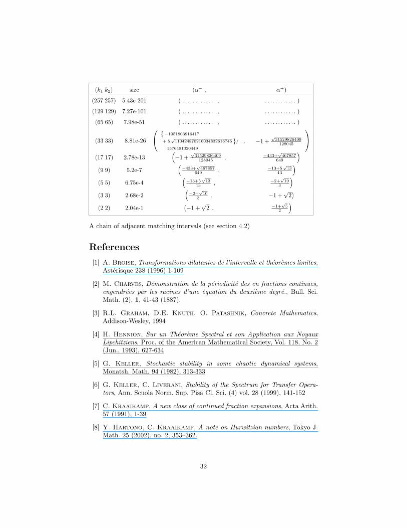
4.2 Adjacent intervals and period doubling
Let us now focus on pairs of adjacent intervals (corresponding to isolated pointsin [0, 1]\M): our data show they all come in infinite chains, and can be obtainedfrom some starting matching interval via a “period doubling” construction.
23
Let’s start with a matching interval ]α, β[ ; α = [0;S ] where S is a sequence ofpositive integer of odd length; define the sequence of strings{
S0 = SSn+1 = (SnSn)′ (3)
where S′ denotes the conjugate of S as in def. 4.1. Let an := [0;Sn] andbn := [0;S′n]; then the sequence In :=]an, bn[ is formed by a chain of adjacentintervals: clearly bn+1 = an, moreover an < bn because |Sn| is odd for all n.
Assuming this scheme, we can construct many cluster points of matchingintervals. For instance, let us look at the first (i.e. rightmost) one: we startwith the interval ](
√5− 1)/2, 1[ so that the first terms of the sequence Sn are
S0 = (1)S1 = (2)S3 = (2, 1, 1)S4 = (2, 1, 1, 2, 2)S5 = (2, 1, 1, 2, 2, 2, 1, 1, 2, 1, 1)
The corresponding sequence an converges to the first (i.e. rightmost) pointα where intervals of matching cluster. We can also determine the continuedfraction expansion of the value α, since it can be obtained just merging9 thestrings (Sn)n ∈ Nα = [0, 2, 1, 1, 2, 2, 2, 1, 1, 2, 1, 1, 2, 1, 1, 2, 2, 2, 1, 1, 2, 2, 2, 1, 1, 2, 2, 2, 1, 1, 2, 1, 1, 2, 1, 1, 2, 2, 2, ...]
Numerically10, α ∼= 0.386749970714300706171524803485580939661. . .It is evident from formula (3) that any such cluster point will be a bounded-
type number; one can indeed prove that no cluster point of this type is aquadratic surd.
5 Behaviour of entropy inside the matching set
In [12], the following formula is used to relate the change of entropy betweentwo sufficiently close values of α to the invariant measure corresponding to oneof these values: more precisely
Proposition 5.1. Let us suppose the hypotheses of prop. 3.1 hold for α: thenfor η > 0 small enough
h(Tα−η) =h(Tα)
1 + (k2 − k1)µα([α− η, α])(4)
and similarly
h(Tα) =h(Tα+η)
1 + (k2 − k1)µα+η([α, α+ η])(5)
By exploiting these formulas, we will get some results on the behaviour ofh(Tα).
9This can be done since, by (3), Sn is a substring of Sn+1.10This pattern has been checked up to level 10, which corresponds to a matching interval
of size smaller than 10−200; see also the second table in section 6.1.
24
5.1 One-sided differentiability of h(Tα)
Equation (4) has interesting consequences on the differentability of h: we canrewrite it as
h(Tα)− h(Tα−η) = h(Tα−η)(k2 − k1)µα([α− η, α])
and dividing by η
h(Tα)− h(Tα−η)η
= h(Tα−η)(k2 − k1)µα([α− η, α])
η
Since ρα has bounded variation, then there exists R(α) = limx→α− ρα(x), there-fore
limη→0
µα([α− η, α])η
= R(α)
and by the continuity of h (which is obvious in this case by equation (4))
limη→0
h(Tα)− h(Tα−η)η
= h(Tα)(k2 − k1) limx→α−
ρα(x)
hence the function α 7→ h(Tα) is left differentiable in α. On the other hand, onecan slightly modify the proof of (5) and realize it is equivalent to
h(Tα+η) =h(Tα)
1 + (k1 − k2)µα([α− 1, α− 1 + η])
which reduces to
h(Tα+η)− h(Tα)η
=µα([α− 1, α− 1 + η])
η
h(Tα)(k2 − k1)1 + (k1 − k2)µα([α− 1, α− 1 + η])
Since the limit
limη→0
µα([α− 1, α− 1 + η])η
= limx→(α−1)+
ρα(x)
also exists, then h(Tα) is also right differentiable in α, more precisely
limη→0
h(Tα+η)− h(Tα)η
= h(Tα)(k2 − k1) limx→(α−1)+
ρα(x)
We conjecture that in such points the left and right derivatives are equal.This is trivial for k1 = k2; for k1 6= k2 it is equivalent to say limx→α− ρα(x) =limx→(α−1)+ ρα(x).
25
5.2 The entropy for α ≥ 25
Corollary 5.2. For 25 ≤ α ≤
√2− 1, the entropy is
h(Tα) =π2
6 log(√
5+12
)Proof. Every α in the interval (0.4,
√2− 1) satisfies the hypotheses of the the-
orem with k1 = k2 = 3, hence h(Tα) is locally constant, and by continuityh(Tα) = h(T√2−1), whose value was already known.
Remark. By using our computer-generated matching intervals, we can analo-gously prove h(Tα) = h(T√2−1) for
√2− 1 ≥ α ≥ 0.386749970714300706171524...
5.3 Invariant densities
In the case α ≥√
2− 1 it is known that invariant densities are of the form
ρα(x) =r∑i=1
χIi(x)Ai
x+Bi
where the Ii are subintervals of [α− 1, α].For these values of α, a matching condition is present and the endpoints of
the Ii (i.e. the values where the density may “jump”) correspond exactly tothe first few iterates of α and α − 1 under the action of Tα. We present somenumerical evidence in order to support the
Conjecture 5.3. Let α ∈ [0, 1] be a value such that one has a matching of type(k1, k2) (i.e. with T k1α (α) = T k2α (α − 1)). Then the invariant density has theform
ρα(x) =r∑i=1
χIi(x)Ai
x+Bi(6)
where each Ii is an interval with endpoints contained in the set
S := {Tmα (α) : 0 ≤ m < k1} ∪ {Tnα (α− 1) : 0 ≤ n < k2}
Therefore, the number of branches is bounded above by k1 + k2 − 1.
In all known cases, moreover, there exists exactly one Ii which contains αand exactly one which contains α− 1; thus, on neighbourhoods of α and α− 1,the invariant density has the simple form ρα|Ii(x) = Ai
x+BiAs an example of such numerical evidence we report a numerical simulation
of the invariant density for some values of α in the interval [√
13−32 ,
√3−12 ] where
a matching of type (2, 3) occurs. We fit the invariant density with the functionA+/(x + B+) on the interval [max{S}, α] and with the function A−/(x + B−)on [α− 1,min{S}].
26
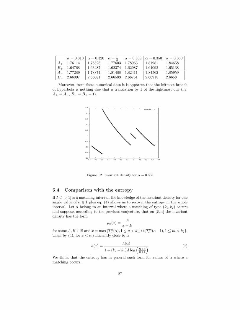
α = 0.310 α = 0.320 α = 13 α = 0.338 α = 0.350 α = 0.360
A+ 1.76114 1.76525 1.77603 1.78963 1.81981 1.84658B+ 1.64768 1.63487 1.62374 1.62987 1.64092 1.65138A− 1.77289 1.78874 1.81488 1.82411 1.84562 1.85959B− 2.66097 2.66081 2.66583 2.66751 2.66915 2.6658
Moreover, from these numerical data it is apparent that the leftmost branchof hyperbola is nothing else that a translation by 1 of the rightmost one (i.e.A+ = A−, B− = B+ + 1).
0.8
0.85
0.9
0.95
1
1.05
1.1
1.15
1.2
1.25
-0.7 -0.6 -0.5 -0.4 -0.3 -0.2 -0.1 0 0.1 0.2 0.3 0.4
inv density
Figure 12: Invariant density for α = 0.338
5.4 Comparison with the entropy
If I ⊂ [0, 1] is a matching interval, the knowledge of the invariant density for onesingle value of α ∈ I plus eq. (4) allows us to recover the entropy in the wholeinterval. Let α belong to an interval where a matching of type (k1, k2) occursand suppose, according to the previous conjecture, that on [x, α] the invariantdensity has the form
ρα(x) =A
x+B
for some A,B ∈ R and x = max{Tnα (α), 1 ≤ n < k1}∪{Tmα (α−1), 1 ≤ m < k2}.Then by (4), for x < α sufficiently close to α
h(x) =h(α)
1 + (k2 − k1)A log(B+αB+x
) (7)
We think that the entropy has in general such form for values of α where amatching occurs.
27
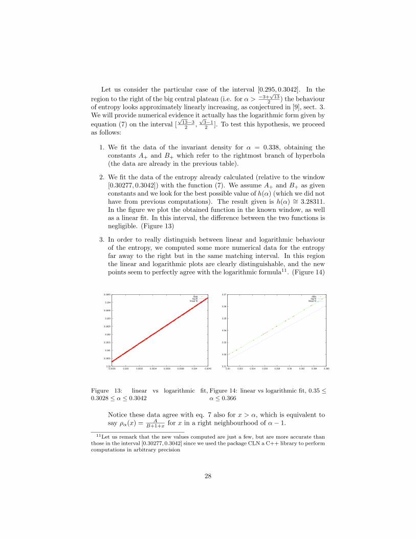
Let us consider the particular case of the interval [0.295, 0.3042]. In theregion to the right of the big central plateau (i.e. for α > −3+
√13
2 ) the behaviourof entropy looks approximately linearly increasing, as conjectured in [9], sect. 3.We will provide numerical evidence it actually has the logarithmic form given byequation (7) on the interval [
√13−32 ,
√3−12 ]. To test this hypothesis, we proceed
as follows:
1. We fit the data of the invariant density for α = 0.338, obtaining theconstants A+ and B+ which refer to the rightmost branch of hyperbola(the data are already in the previous table).
2. We fit the data of the entropy already calculated (relative to the window[0.30277, 0.3042]) with the function (7). We assume A+ and B+ as givenconstants and we look for the best possible value of h(α) (which we did nothave from previous computations). The result given is h(α) ∼= 3.28311.In the figure we plot the obtained function in the known window, as wellas a linear fit. In this interval, the difference between the two functions isnegligible. (Figure 13)
3. In order to really distinguish between linear and logarithmic behaviourof the entropy, we computed some more numerical data for the entropyfar away to the right but in the same matching interval. In this regionthe linear and logarithmic plots are clearly distinguishable, and the newpoints seem to perfectly agree with the logarithmic formula11. (Figure 14)
3.18
3.1805
3.181
3.1815
3.182
3.1825
3.183
3.1835
3.184
3.1845
0.3028 0.303 0.3032 0.3034 0.3036 0.3038 0.304 0.3042
datalog fit
linear fit
Figure 13: linear vs logarithmic fit,0.3028 ≤ α ≤ 0.3042
3.31
3.32
3.33
3.34
3.35
3.36
3.37
0.35 0.352 0.354 0.356 0.358 0.36 0.362 0.364 0.366
datalog fit
linear fit
Figure 14: linear vs logarithmic fit, 0.35 ≤α ≤ 0.366
Notice these data agree with eq. 7 also for x > α, which is equivalent tosay ρα(x) = A
B+1+x for x in a right neighbourhood of α− 1.
11Let us remark that the new values computed are just a few, but are more accurate thanthose in the interval [0.30277, 0.3042] since we used the package CLN a C++ library to performcomputations in arbitrary precision
28
6 Appendix
In this appendix we give the proof of two simple results which are of somerelevance for the issues discussed in this paper.
Proposition 6.1. If x0 is a quadratic surd then x0 is a preperiodic point forTα, α ∈ [0, 1].
For α = 1 this is the well known Lagrange Theorem, and this statement isknown to be true for α = 0 and α ∈ [1/2, 1] [8]. Since we did not find a referencecontaining a simple proof of this fact for all α ∈ [0, 1] we sketch it here, infew lines: this proof follows closely the classical proof of Lagrange Theorem forregular continued fractions given by [2] which relies on approximation propertiesof convergents, therefore it works for α > 0.
If x0 is a quadratic surd then F0(x0) = 0 for some F0(x) := A0x2 + B0x +
C0 quadratic polynomial with integer coefficients. On the other hand, since12
x0 = pn−1xn+pnqn−1xn+qn
, setting Fn(x) := F0(pn−1x+pnqn−1x+qn
)(qn−1x + qn)2, we get thatFn(xn) = F0(x0) = 0.
Moreover Fn(x) = Anx2 +Bnx+ Cn with
An = F0(pn−1/qn−1)q2n−1, Cn = F0(pn/qn)q2
n, B2n − 4AnCn = B2
0 − 4A0C0.(8)
Both An, Bn are bounded since: |F0(pn/qn)| = |F0(pn/qn) − F0(x0)| =|F ′0(ξ)||pnqn − x0| ≤ C
αq2n; moreover from the last equation in (8) it follows that
Bn are bounded as well.
Proposition 6.2. The variance σ2(α) is constant for α ∈ [√
2−1, (√
5−1)/2].
This result relies on the fact that for all α ∈ [√
2−1, (√
5−1)/2] the maps Tαhave natural extensions Tα which are all isomorphic to T1/2. In the followingwe shall prove the claim for α ∈ [
√2 − 1, 1/2] and we shall write T1 instead
of Tα and T2 instead of T1/2. So Tj : Ij → Ij , (j = 1, 2) are 1-dimensionalmap with invariant measure µj ; Tj : Ij → Ij , (j = 1, 2) are the corresponding2-dimensional representations of the natural extension with invariant measureµj , and Φ : I1 → I2 is the (measurable) isomorphism
Φ ◦ T1 = T2 ◦ Φ, Φ∗µ1 = µ2
First let us point out (see [12] pg 1222-1223) that Φ is almost everywhere dif-ferentiable and has a diagonal differential; moreover Tj are almost everywheredifferentiable as well and have triangular differential. Therefore
dΦ|T1(x,y)dT1|(x,y) = dT2|Φ(x,y)dΦ(x,y) (9)
and it ie easy to check that, setting T xj the first component of Tj , a scalaranalogue holds as well
∂Φx
∂x|T1(x,y)
∂T x1∂x|(x,y) =
∂T x2∂x|Φ(x,y)
∂Φx
∂x|(x,y) (10)
12To simplify notations we shall write pn, qn instead of pn,α, qn,α.
29
So we get that, for all k,
log
∣∣∣∣∣∂T x1∂x∣∣∣∣∣ = log
∣∣∣∣∣∂T x2∂x ◦ Φ
∣∣∣∣∣+ log∣∣∣∣∂Φx
∂x
∣∣∣∣− log∣∣∣∣∂Φx
∂x◦ T1
∣∣∣∣Since T x1 is µ1-measure preserving
∫I1
log∣∣∂Φx
∂x
∣∣− log∣∣∣∂Φx
∂x ◦ T1
∣∣∣ dµ1 = 0; so,taking into account that Φµ1 = µ2 we get
∫I1
log
∣∣∣∣∣∂T x1∂x∣∣∣∣∣ dµ1 =
∫I1
log
∣∣∣∣∣∂T x2∂x ◦ Φ
∣∣∣∣∣ dµ1 =∫I2
log
∣∣∣∣∣∂T x2∂x∣∣∣∣∣ dµ2 := m.
Let us define g1 := log∣∣∣∂Tx1∂x ∣∣∣ and g2 := log
∣∣∣∂Tx2∂x ∣∣∣ (so that∫I1g1dµ1 =∫
I2g2dµ2 = 0) and STNg :=
∑N−1k=0 g ◦ T k; we easily see that
ST1N g1 = ST2
N g1 ◦ Φ log∣∣∣∣∂Φx
∂x◦ T k1
∣∣∣∣− log∣∣∣∣∂Φx
∂x◦ T k+1
1
∣∣∣∣which means that ST1
N g1 and ST2N g2 ◦ Φ differ by a coboundary.
Lemma 6.3. Let u, v be two observables such that
1. limN→+∞∫
(SNv√N
)2dµ = l ∈ R;
2. u = v + (f − f ◦ T ) for some f ∈ L2.
Thenlim
N→+∞
∫(SNv√N
)2dµ = limN→+∞
∫(SNu√N
)2dµ.
The lemma implies
limN→+∞
ZI1
ST1N g1√N
!2
dµ1 = limN→+∞
ZI2
ST2N g2√N
!2
dµ2 (11)
This information can be translated back to the original systems: since ∂Tx1∂x |(x,y) =
T ′1(x), ∂Tx2∂x |(x,y) = T ′2(x) if we define
G1 := log |T ′1(x)| −∫I1
log |T ′1(x)|dµ1
G2 = log |T ′2(x)| −∫I2
log |T ′2(x)|dµ2
we get g1(x, y) = G1(x) and g2(x, y) = G2(x); therefore ST1N g1 = ST1
N G1 andST2N g2 = ST2
N G2. Finally, by equation (11), we get
limN→+∞
∫I1
(ST1N G1√N
)2
dµ1 = limN→+∞
∫I2
(ST2N G2√N
)2
dµ2
30
6.1 Tables
(k1 k2) size (α− , α+) (k1 k2) size (α− , α+)
(3 9) 7.69e-4(−8+
√82
9 , −2+√
52
)(8 6) 6.42e-5
(−33+
√2305
64 , −77+√
722134
)(2 8) 3.68e-3
(−4 +
√17 , −7+
√77
14
)(5 5) 1.46e-3
(−7+
√101
13 , −2 +√
5)
(3 8) 1.11e-3(−7+
√65
8 , −7+3√
77
)(2 4) 2.77e-2
(−2 +
√5 , −3+
√21
6
)(2 7) 5.44e-3
(−7+
√53
2 , −3+√
156
)(3 6) 2.1e-3
(−7+
√65
4 , −6+4√
511
)(3 8) 6.98e-4
(−19+
√445
14 , −9+2√
3013
)(4 6) 7.02e-4
(−11+
√226
15 , −23+3√
9322
)(3 7) 1.69e-3
(−6+5
√2
7 , −3+2√
33
)(3 5) 3.97e-3
(−5+
√37
4 , −9+√
16514
)(4 7) 8.12e-4
(−17+
√445
26 , −3+√
112
)(4 6) 5.77e-4
(−13+
√257
11 , −2+2√
23
)(2 6) 8.54e-3
(−3 +
√10 , −5+3
√5
10
)(4 5) 1.51e-3
(−15+
√445
22 , −8+3√
117
)(3 8) 6.06e-4
(−11+
√145
6 , −10+2√
4217
)(5 5) 7.88e-4
(−10+
√226
18 , −23+5√
2914
)(3 7) 1.12e-3
(−8+
√82
6 , −15+√
35722
)(3 4) 1.02e-2
(−3+
√17
4 , −3+√
153
)(3 6) 2.76e-3
(−5+
√37
6 , −5+√
355
)(4 6) 8.86e-4
(−11+
√170
7 , −19+3√
9334
)(4 6) 1.34e-3
(−7+
√82
11 , −15+√
28510
)(4 5) 1.78e-3
(−15+
√365
14 , −7+3√
1110
)(9 7) 2.38e-5
(−51+13
√29
100 , −117+√
1562142
)(5 5) 7.09e-4
(−11+
√257
17 , −6+2√
145
)(5 6) 7.91e-4
(−9+
√145
16 , −10+2√
305
)(8 6) 2.73e-5
(−54+
√7057
101 , −127+7√
45374
)(9 7) 2.25e-5
(−53+
√5185
99 , −30+4√
6613
)(4 4) 5.24e-3
(−4+
√37
7 , −3+√
132
)(10 7) 1.54e-5
(−127+
√30629
250 , −73+√
608326
)(8 6) 2.73e-5
(−54+
√7057
101 , −127+7√
45374
)(2 5) 1.45e-2
(−5+
√29
2 , −1+√
22
)(2 3) 6.32e-2
(−3+
√13
2 , −1+√
32
)(3 8) 6.57e-4
(−23+
√629
10 , −10+√
19519
)(4 6) 6.9e-4
(−13+
√290
11 , −23+√
136538
)(3 7) 1.06e-3
(−9+
√101
5 , −4+√
307
)(4 5) 1.72e-3
(−15+
√533
22 , −4+√
304
)(3 6) 1.98e-3
(−13+
√229
10 , −2+√
73
)(3 4) 9.87e-3
(−7+
√85
6 , −3+2√
65
)(4 6) 7.42e-4
(−10+
√170
14 , −7+√
696
)(4 5) 1.45e-3
(−9+
√145
8 , −8+2√
4213
)(9 7) 1.03e-5
(−81+
√13226
155 , −187+3√
466982
)(4 4) 3.82e-3
(−5+
√65
8 , −11+√
22110
)(3 5) 4.94e-3
(−4+
√26
5 , −2+√
62
)(5 5) 6.75e-4
(−13+5
√13
13 , −2+√
103
)(4 6) 8.44e-4
(−10+
√145
9 , −19+3√
6926
)(3 3) 2.68e-2
(−2+
√10
3 , −1 +√
2)
(7 6) 1.11e-4(−25+
√1297
48 , −29+√
102313
)(2 2) 2.04e-1
(−1 +
√2 , −1+
√5
2
)(4 5) 2.45e-3
(−11+
√229
18 , −3+2√
32
)(2 1) 3.82e-1
(−1+
√5
2 , 1]
A sample of matching intervals found as in section 4.
31
(k1 k2) size (α− , α+)
(257 257) 5.43e-201 ( . . . . . . . . . . . . , . . . . . . . . . . . . )
(129 129) 7.27e-101 ( . . . . . . . . . . . . , . . . . . . . . . . . . )
(65 65) 7.98e-51 ( . . . . . . . . . . . . , . . . . . . . . . . . . )
(33 33) 8.81e-26
{−1051803916417
+ 5√
110424870216034832616745 }/1576491320449
, −1 +√
31529826409128045
(17 17) 2.78e-13
(−1 +
√31529826409
128045 , −433+√
467857649
)(9 9) 5.2e-7
(−433+
√467857
649 , −13+5√
1313
)(5 5) 6.75e-4
(−13+5
√13
13 , −2+√
103
)(3 3) 2.68e-2
(−2+
√10
3 , −1 +√
2)
(2 2) 2.04e-1(−1 +
√2 , −1+
√5
2
)A chain of adjacent matching intervals (see section 4.2)
References
[1] A. Broise, Transformations dilatantes de l’intervalle et theoremes limites,Asterisque 238 (1996) 1-109
[2] M. Charves, Demonstration de la periodicite des en fractions continues,engendrees par les racines d’une equation du deuxieme degre., Bull. Sci.Math. (2), 1, 41-43 (1887).
[3] R.L. Graham, D.E. Knuth, O. Patashnik, Concrete Mathematics,Addison-Wesley, 1994
[4] H. Hennion, Sur un Theoreme Spectral et son Application aux NoyauxLipchitziens, Proc. of the American Mathematical Society, Vol. 118, No. 2(Jun., 1993), 627-634
[5] G. Keller, Stochastic stability in some chaotic dynamical systems,Monatsh. Math. 94 (1982), 313-333
[6] G. Keller, C. Liverani, Stability of the Spectrum for Transfer Opera-tors, Ann. Scuola Norm. Sup. Pisa Cl. Sci. (4) vol. 28 (1999), 141-152
[7] C. Kraaikamp, A new class of continued fraction expansions, Acta Arith.57 (1991), 1-39
[8] Y. Hartono, C. Kraaikamp, A note on Hurwitzian numbers, Tokyo J.Math. 25 (2002), no. 2, 353–362.
32
[9] L. Luzzi, S. Marmi, On the entropy of Japanese continued frac-tions, Discrete and continuous dynamical systems, 20 (2008), 673-711,arXiv:math.DS/0601576v2
[10] A. Cassa, P. Moussa, S. Marmi, Continued fractions and Brjuno func-tions, J. Comput. Appl. Math. 105 (1995), 403-415
[11] H. Nakada, Metrical theory for a class of continued fraction transforma-tions and their natural extensions, Tokyo J. Math. 4 (1981), 399-426
[12] H. Nakada, R. Natsui, The non-monotonicity of the entropy of α-continued fraction transformations, Nonlinearity 21 (2008), 1207-1225
[13] V.A. Rohlin, Exact endomorphisms of a Lebesgue space, Izv. Akad. NaukSSSR Ser. Mat. 25 (1961), 499-530; English translation: Amer. Math. Soc.Transl. (2) 39 (1964), 1-36
[14] M. Rychlik, Bounded variation and invariant measures, Studia Math. 76(1983), 69-80
[15] F. Schweiger, Ergodic theory of fibred systems and metric number theory,Oxford Sci. Publ. Clarendon Press, Oxford, 1995
[16] G.Tiozzo The entropy of α-continued fractions: analytical results, preprint
[17] M. Viana, Stochastic Dynamics of Deterministic Systems, Lecture NotesXXI. Braz. Math. Colloq. IMPA, Rio de Janeiro, 1997
[18] R. Zweimuller, Ergodic structure and invariant densities of non-Markovian interval maps with indifferent fixed points, Nonlinearity 11(1998), 1263-1276
Dipartimento di Matematica, Universita di Pisa, Largo Bruno Pon-tecorvo 5, 56127 Pisa, Italy. e-mail: [email protected] Normale Superiore, Piazza dei Cavalieri 7, 56123 Pisa, Italy. e-mail: [email protected] Normale Superiore, Piazza dei Cavalieri 7, 56123 Pisa, Italy. e-mail: [email protected] of Mathematics, Harvard University, 1 Oxford St, Cam-bridge MA 02138, U.S.A. e-mail: [email protected]
33


