Continued Fractions and the 4-Color Theorem

Richard Evan Schwartz ∗

October 26, 2022

Abstract

We study the geometry of some proper 4-colorings of the verticesof sphere triangulations with degree sequence 6, ..., 6, 2, 2, 2. Such tri-angulations are the simplest examples which have non-negative com-binatorial curvature. The examples we construct, which are roughlyextremal in some sense, are based on a novel geometric interpreta-tion of continued fractions. We will also present a conjectural sharp“isoperimetric inequality” for colorings of this kind of triangulation.

1 Introduction

1.1 Background

The Four Color Theorem, first proved (with the assistance of a computer)by Wolfgang Haken and Kenneth Appel in 1976, is one of the most famousresults in mathematics. See [W] for a thorough discussion. Here is oneformulation. If you have any triangulation of the 2-sphere, it is possible tocolor the vertices using 4 colors such that no two adjacent vertices have thesame coloring. This is called a proper vertex 4-coloring .

Certainly one can properly 4-color the vertices of a tetrahedron. A propervertex 4-coloring of a triangulation Z (with the same colors) canonicallydefines a simplicial map f from the sphere to the tetrahedron: Just mapeach vertex of Z to the like-colored vertex of the tetrahedron and then extendlinearly to the faces. The map f in turn defines a 2-coloring of the faces of

∗Supported by N.S.F. Grant DMS-2102802

1

Z. One colors a face of Z black if f is orientation preserving on that face,and otherwise white.

The associated face 2-coloring has the property that around each ver-tex the number of black faces is congruent mod 3 to the number of whitefaces. This derives from the property that 3 triangles of the tetrahedronmeet around each vertex. We call a face 2-coloring with this property a goodcoloring . Conversely, a good coloring for Z defines a simplicial map to thetetrahedron and thus a proper 4-coloring of the vertices of Z. So, an equiv-alent formulation of the 4-color theorem is that every triangulation of thesphere has a good coloring.

So far, the Four Color Theorem only has computer-assisted proofs. Per-haps one can get insight into the result by looking at examples of goodcolorings. The good coloring version has a geometric feel to it, and so per-haps some geometric insight might help. The purpose of this paper is to lookat the geometry of these good colorings in some special cases.

A triangulation of non-negative combinatorial curvature is one in whichthe maximum degree is 6. All the vertices have degree 6 except for a listv1, ..., vk which have degrees d1, ..., dk < 6. Euler’s Formula gives the condi-tion on the degrees:

k∑i=1

(6− di) = 12. (1)

In particular k ≤ 12. The quantity

π

3× (6− di)

is the combinatorial curvature at vi. Equation 1 translates into a discreteversion of the Gauss-Bonnet theorem, which says that the total combinatorialcurvature is 4π.

The triangulations of non-negative combinatorial curvature form an at-tractive family to study. In [T], William Thurston organized these triangu-lations into moduli spaces. To give some idea of how this works, a triangula-tion non-negative combinatorial curvature defines a flat cone structure on thesphere with non-negative curvature: we just make all the triangles unit equi-lateral triangles. The set of all triangulations with the same list d1, .., dk ofdefects includes in the moduli space of flat cone structures on spheres withappropriately prescribed singularities. So, even though the triangulationsdon’t exactly vary continuously, one can think of them as special points in-side moduli spaces consisting of structures which do vary continuously. Also,

2

if the triangulations are large and the defects are well spread out, one canimagine that the defects almost vary continuously.

Given the nice structure of the totality of such triangulations, it seemslike an interesting idea to study the space of good colorings as a kind ofpartially defined bundle over these moduli spaces. Perhaps the structureof such colorings is related somehow to the placement of the defects. Asthe defects vary around, perhaps the good colorings vary in a nice way tosome extent. I imagine that the total picture, seen all at once, would bespectacularly beautiful. All this is very speculative. In spite of making a lotof computer experiments over the years – every time I teach the graph theoryclass at Brown I play with this project – I don’t have much to report. Inthis very modest paper I will consider the simplest cases. The cases I havein mind are where k = 3 and d1 = d2 = d3 = 2.

1.2 The Continued Fraction Colorings

The 6, ..., 6, 2, 2, 2 trianglulations are indexed by the nonzero Eisenstein in-tegers. An Eisenstein integer is a number of the form

a+ bα, a, b ∈ Z, α =1 + i

√3

2.

(It is more common to use ω = α2 in place of α, but α is more convenient forus.) To see the connection, let E denote the ring of Eisenstein integers. Thepoints of E are naturally the vertices of an equilateral triangulation T of C.Given some nonzero β ∈ E , we let βT be the bigger equilateral triangulationobtained by multiplying the whole picture by β. We let Gβ denote the groupof symmetries generated by order 3 rotations in the vertices of βT . Thequotient

T (β) = T /Gβ

is the desired triangulation.Since all the vertices of T (β) have even degree, T (β) always has a good

coloring. One just colors the triangles alternately black and white in acheckerboard pattern. Indeed, this face coloring corresponds to a proper3-coloring of the vertices.

Figure 1 shows a different good coloring for β = 2 + 3α. We call thiscoloring C(2+3α). To get the triangulation of the sphere, cut out the speciallyoutlined central rhombus, fold it up like a taco, and glue the edges together

3

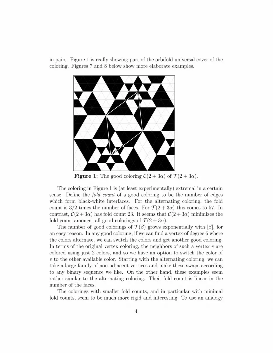
in pairs. Figure 1 is really showing part of the orbifold universal cover of thecoloring. Figures 7 and 8 below show more elaborate examples.

Figure 1: The good coloring C(2 + 3α) of T (2 + 3α).

The coloring in Figure 1 is (at least experimentally) extremal in a certainsense. Define the fold count of a good coloring to be the number of edgeswhich form black-white interfaces. For the alternating coloring, the foldcount is 3/2 times the number of faces. For T (2 + 3α) this comes to 57. Incontrast, C(2 + 3α) has fold count 23. It seems that C(2 + 3α) minimizes thefold count amongst all good colorings of T (2 + 3α).

The number of good colorings of T (β) grows exponentially with |β|, foran easy reason. In any good coloring, if we can find a vertex of degree 6 wherethe colors alternate, we can switch the colors and get another good coloring.In terms of the original vertex coloring, the neighbors of such a vertex v arecolored using just 2 colors, and so we have an option to switch the color ofv to the other available color. Starting with the alternating coloring, we cantake a large family of non-adjacent vertices and make these swaps accordingto any binary sequence we like. On the other hand, these examples seemrather similar to the alternating coloring. Their fold count is linear in thenumber of the faces.

The colorings with smaller fold counts, and in particular with minimalfold counts, seem to be much more rigid and interesting. To use an analogy

4

from statistical mechanics, the colorings with large fold count are sort of likea fluid or a gas, and the colorings with small fold count are more like solidcrystals. The example in Figure 1 is part of an infinite sequence of examples.We call these examples C(β), where β ranges over the primitive Eisensteinintegers. (An Eisenstein integer β = a + bα primitive if it is not an integermultiple of another one. Equivalently, a and b are relatively prime.) Wewill see that C(β) is a special good coloring of T (β) which geometricallyimplements the continued fraction expansion of a/b. We call these coloringscontinued fraction colorings .

1.3 Properties of the Continued Fraction Colorings

The main result of this paper is that these continued fraction colorings exist,but I will prove some additional results about them. One interesting propertyis that these colorings have the same number of black and white triangles.See §3.1 for the quick proof, which I learned from Kasra Rafi.

Our next result concerns the asymptotics of the fold count (and of anotherquantity) for the continued fraction colorings. Let an/bn ∈ (0, 1) be asequence of rationals. Let

T n = T (an + bnα), Cn = C(an + bnα).

Let fn denote the fold count of Cn and let Fn denote the number of faces inT n. Let Rn denote the radius of the largest monochrome disk contained inCn. When Rn is large, it means that Cn contains large totally solid chunks.

Theorem 1.1 The following is true about the continued fraction colorings.

1. If an/bn converges to an irrational limit then limn→∞ fn/Fn = 0.

2. If an/bn converges to an irrational limit then limn→∞Rn =∞.

3. If an/bn is the sequence of continued fraction approximants of aquadratic irrational, then limn→∞f 2

n/Fn exists and is finite.

Statement 3 of Theorem 1.1 motivates the following definitions.

Definition: Given a coloring C we define

η(C) =f 2

F, (2)

5

where f is the fold count for C and F is the number of triangles in the trian-gulation which C colors. We call η(C) the Eisenstein Isoperimetric Ratio of C.

Definition: Given a quadratic irrational η ∈ (0, 1) let

η(ζ) = limn→∞

η(pn + qnα),

where pn/qn is the sequence of continued fraction approximants of ζ. Wecall η(ζ) the Eisenstein Isoperimetric Ratio of ζ.

In §3.3 we will show, among other calculations, that

η(φ−1) = φ6, φ =

√5 + 1

2. (3)

Here φ is the golden ratio. Our proof of Statement 3 of Theorem 1.1 willshow more generally that η(ζ) ∈ Q(ζ), the quadratic field containing ζ. See§3.3 for some examples.

For comparison we prove the following easy result.

Theorem 1.2 Let C be any good coloring of any triangulation with degreesequence 6, ..., 6, 2, 2, 2. Then η(C) ≥ 3.

Theorem 1.2 indicates that some of the continued fraction colorings roughlyminimize the fold count. Here is a strong conjecture along these lines.

Conjecture 1.3 Suppose Gn is any infinite sequence of distinct coloringsof primitive sphere triangulations with degree sequence 6, ..., 6, 2, 2, 2. Thenlim infn→∞ η(Gn) ≥ φ6.

Here primitive means that the triangulation has the form T (β) for a primitiveEisenstein integer β. Equation 3 says that this conjecture is sharp. Sinceφ6 = 17.944... < 18, Theorem 1.2 says that the conjecture is true up to afactor of 6.

Sometimes there are good colorings which have lower fold count then thecorresponding continued fraction coloring. See Figure 9 in §3 for an example.Here is one last conjecture about the general situation.

Conjecture 1.4 There is a constant Ω with the following property. For anytriangulation T with degree sequence 6, ...., 6, 2, 2, 2 there is a good coloringC of T with η(C) < Ω.

6

1.4 Organization

In §2, after a discussion of the slow Gauss map and its connection to con-tinued fractions, I will launch into the construction of the continued fractioncolorings. The building blocks are what I call capped flowers , and these inturn are made in layers from cyclically arranged patterns of trapezoids whichI call trapezoid necklaces . (Look again at Figure 1.) I will explain how theset of trapezoid necklaces is naturally the vertex set of the infinite rootedbinary tree (modified to have an extra vertex at the bottom). Taking a pathin this tree defines the capped flower. In §3 I will prove Theorems ?? and1.1, establish Equation 3, and give some evidence for Conjecture 1.3. In §4I will prove Theorem 1.2.

1.5 Acknowledgements

I’d like to thank Ethan Bove, Peter Doyle, Jeremy Kahn, Rick Kenyon,Curtis McMullen, Kasra Rafi, and Peter Smillie for various conversations(sometimes going back some years) on topics related to the material here.

7

2 The Main Construction

2.1 The Slow Gauss Map

Let S denote the set of rational numbers in the interval (0, 1]. The slowGauss map is the following map from S − 1 into S:

γ

(a

a+ b

)= γ

(b

a+ b

)=a

b. (4)

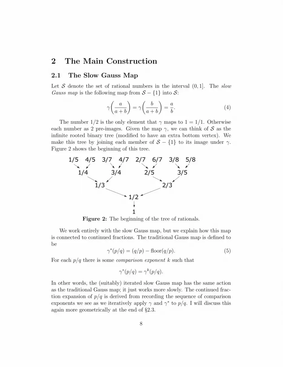
The number 1/2 is the only element that γ maps to 1 = 1/1. Otherwiseeach number as 2 pre-images. Given the map γ, we can think of S as theinfinite rooted binary tree (modified to have an extra bottom vertex). Wemake this tree by joining each member of S − 1 to its image under γ.Figure 2 shows the beginning of this tree.

1

1/2

1/3 2/3

1/4 3/4 2/5 3/5

1/5 4/5 3/8 5/83/7 4/7 2/7 6/7

Figure 2: The beginning of the tree of rationals.

We work entirely with the slow Gauss map, but we explain how this mapis connected to continued fractions. The traditional Gauss map is defined tobe

γ∗(p/q) = (q/p)− floor(q/p). (5)

For each p/q there is some comparison exponent k such that

γ∗(p/q) = γk(p/q).

In other words, the (suitably) iterated slow Gauss map has the same actionas the traditional Gauss map; it just works more slowly. The continued frac-tion expansion of p/q is derived from recording the sequence of comparisonexponents we see as we iteratively apply γ and γ∗ to p/q. I will discuss thisagain more geometrically at the end of §2.3.

8

2.2 Trapezoid Necklaces

An isosceles trapezoid is a quadrilateral with two parallel sides such thatthe other two sides are non-parallel but have the same length. We call thelonger parallel side the top, the shorter parallel side the bottom, and the othertwo sides the diagonal sides . We allow the degenerate case of an isoscelestriangle. In this case the bottom has length 0. An Eisenstein trapezoidis an isosceles trapezoid whose edges lie in the 1-skeleton of T , the planarequilateral triangulation whose vertices are the Eisenstein integers. Figure 1above and Figure 3 below feature some Eisenstein trapezoids.

Up to symmetries of T , an Eisenstein trapezoid X is characterized bythe pair (a, b) where a is the length of a diagonal side of X and b is thelength of the top. We call X primitive if a, b are relatively prime. When X isprimitive, we define the aspect ratio to be a/b. The aspect ratio determinesthe primitive Eisenstein trapezoid up to symmetries of T . Thus, modulosymmetry the primitive Eisenstein trapezoids are naturally in bijection withthe set S of rationals considered above. The Eisenstein trapezoids in Figure1 are all primitive, and their aspect ratios are variously 1/1 and 1/2 and 2/3.The Eisenstein trapezoids in Figure 3 have aspect ratio 3/5.

3+53+5-2+5

3+21+2

Figure 3: A trapezoid necklace of aspect ratio 3/5.

9

Figure 3 illustrates what we mean by a trapezoid necklace. This is aunion of 6 primitive Eisenstein trapezoids X1, ..., X6 which has the followingproperties:

• The trapezoids have pairwise disjoint interiors.

• Xi ∩Xi+1 is a single point, a common vertex, for all i.

• An order 6 rotation ρ of T has the action ρ(Xi) = Xi+1 for all i.

In this description the indices are taken mod 6. We define the center of thenecklace to be the fixed point of ρ. When the center is 0, the map ρ (orperhaps its inverse) is multiplication by α. We define the aspect ratio of thenecklace to be the common aspect ratio of the 6 individual trapezoids.

Up to symmetry of T , there exists a unique Eisenstein necklace of aspectratio a/b ∈ S. If we normalize the picture so that 0 is the center, then oneof the trapezoids X1 has vertices

a+ bα, (a− b) + bα, (2a− b) + (b− a)α, a+ (b− a)α.

The intersection of X1 and X2 = ρ(X1) is the point (a− b) + bα because

α×(a+ (a− b)α) = (a− b) + bα.

This little calculation uses the fact that α2 = α− 1.

2.3 Empty Trapezoid Flowers

Each trapezoid necklace X defines a smaller trapezoid necklace Y = γ(X)having the same center. The defining property is that the top side of eachtrapezoid Yi in Y is a side of a trapezoid Xj of X, and one of the diagonalsides of Yi is a side of one of the trapezoids of X adjacent to Xj. Thisawkward definition is very much like a written description of how to drink aglass of water. A demonstration says a thousand words. Figure 4 shows thetrapezoid necklaces

X → γ(X)→ γ2(X)→ γ3(X)

alternately colored black and white. Here X is as in Figure 3. The respectiveaspect ratios are given by 3/5 → 2/3 → 1/2 → 1/1. We call the union ofthese necklaces the empty 3/5-flower .

10

Figure 4: The empty 3/5-flower.

As is suggested by our notation, the action of γ here mirrors the actionof the slow Gauss map γ from the previous section. That is, if r is the aspectratio of X then γ(r) is the aspect ratio of γ(X). Our construction mirrorsthe action of the slow Gauss map.

We discussed above how the slow Gauss map is related to continued frac-tions. Here we continue the discussion. As we now illustrate, our constructionalso precisely implements the continued fraction expansion.

11

Figure 5: The empty 3/7-flower.

Figure 5 shows the empty 3/7-flower, corresponding to the tree path3/7 → 3/4 → 1/3 → 1/2 → 1/1. The specially-outlined trapezoids (andtheir rotated images) are the maximal trapezoids in the flower. They haverespectively 2 and 3 “stripes”. For comparison, 3/7 has continued fraction0 : 2 : 3. That is

3

7= 0 +

1

2 + 13

.

In general, the empty p/q-flower starts with a p/q-necklace and then fillsin the full γ orbit, alternately coloring the necklaces black and white. Theinnermost necklace always has aspect ratio 1/1. Up to symmetries of T ,the empty p/q-flower is unique. One can read off the continued fractionexpansion of p/q by counting the stripes of the maximal trapezoids.

12

2.4 Filling and Capping the Flowers

We fill an empty flower by coloring the remaining 6 triangles black and whitein an alternating pattern. Figure 6 shows this for the 3/5-flower. Up tosymmetries of T (and swapping the colors) there is a unique p/q-flower. Theempty flowers have 6-fold rotational symmetry but the (filled) flowers have3-fold rotational symmetry. We break a symmetry to define the filling.

Figure 6: The filled and capped 3/5-flower

Figure 6 also shows what we mean by capping a flower. We take theconvex hull of the flower and color the complementary triangles the coloropposite the color of the outer necklace. The capped flowers, which are reg-ular hexagons with Eisenstein integer vertices, are the building blocks of ourcolorings. When two translation-equivalent capped flowers meet along a com-mon boundary edge, the triangular regions merge to become an Eisensteinparallelogram – i.e., one whose boundary lies in the 1-skeleton of T .

13

2.5 Defining the Colorings

Consider the hexagonal tiling of the plane by translates of the capped a/b-flower. Because the capped flowers have 3-fold rotational symmetry, theresulting planar coloring is invariant under the group Gβ generated by order3 reflections in the vertices and centers of the hexagons. The quotient of thisplanar coloring by Gβ is C(β). By construction, C(β) is good.

Figure 7: The universal cover of C(3 + 5α).

Figure 7 shows the construction for β = 3 + 5α. The region boundedby the big central rhombus is a fundamental domain for the action of Gβ.The colorings exhibit a lot of variety. Figure 8 below shows C(a + 13b) fora = 1, 3, 5, 7, 9, 11. It is worth noting that for parameters like 1/13 the foldcount is linear in the number of triangles.

14

Figure 8: The covers of C(a+ 13α) for a = 1, 3, 5, 7, 9, 11..

15

3 Properties of the Colorings

3.1 Zero Degree

Let T denote the regular tetrahedron. Call a triangulation of the sphere evenif it has all even degrees. In this section we prove that any good coloring of aneven triangulation Σ has the same total number of black and white triangles.This is equivalent to the statement that the associated map f : Σ → T hastopological degree 0. I learned this proof from Kasra Rafi.

We equip R2 with the unit equilateral triangulation. Let π : R2 → T bethe branched covering which maps triangles to triangles in an affine way. Agood triangulation has the property that, around each vertex, the number ofblack triangles is congruent mod 3 to the number of white triangles. In thecase of an even triangulation, a good coloring has the stronger property thataround each vertex the number of black triangles is congruent mod 6 to thenumber of white triangles. But this means that the map f : Σ → T lifts toa map f : Σ→ R2 such that f = π f . The map f is homotopic to a pointand hence so is f . But then f has topological degree 0.

3.2 Asymptotic Properties

In this section we prove Theorem 1.1.Now suppose that pn/qn is an infinite sequence of elements of S having

an irrational limit ψ. The continued fraction expansions of these numbersconverge to the continued fraction expansion of ψ. This means that for anyD there are constants M,N such that if n > N then all but the first Mterms of pn/qn have pn > D. In terms of the flowers, all but the first M innertrapezoid necklaces Q have the property that

p(Q)

A(Q)<

100

D.

Here p(Q) denotes the perimeter of Q and, as above, A(Q) denotes thenumber of equilateral triangles comprising Q. We picked an unrealisticallylarge constant of 100 here to avoid having to think about the fine points oftrapezoids.

Our analysis shows that, within the nth flower, the average ratio of theperimeter of a trapezoid to the area of the trapezoid tends to 0 as n → ∞.

16

This immediately implies that the ratio fn/Fn converges to 0. This is thefirst property.

The second property is immediate. The big and fat trapezoids in ourflowers will contain big monochrome disks.

Now we turn to the third property. Recall that the quadratic irrationallimit ζ = lim pn/qn has an eventually periodic continued fraction approxima-tion. The fact that the continued fraction expansion is eventually periodictranslates to the fact that our colorings are asymptotically self-similar.

To make this precise, we think of T (pn + qnα) as a coloring of a doubledequilateral triangle. We then scale the metric by a factor of q−1n . The cor-responding sequence of doubled equilateral triangles converges (say, in theGromov-Hausdorff topology) to another doubled equilateral triangle, namely

C/Gβ, β = ζ + α.

Again, Gβ is the group generated by order 3 rotations in the points of theideal E(ζ + α).

The rescaled colorings also converge. The limiting coloring is made from“infinite flowers” and parallelograms. The infinite flowers are limits of therescaled flowers associated to the Eisenstein integers rationals an + bnα. Oneof the trapezoids in the outermost trapezoid necklace in one of these infiniteflowers (with viewed in the plane) has top right vertex β and horizontal topand bottom. The top has length 1 and diagonal sides have length ζ. Theremaining trapezoids also converge. The flower consists of an infinite unionof nested trapezoid necklaces converging to a single point, the origin. Let Fdenote the infinite flower.

Let F [k] denote the infinite flower obtained by trimming off the outermostk trapezoid necklaces of F . The pre-periodicity of the continued fractionexpansion is equivalent to the pre-periodicity of the Gauss map. This meansthat there are integers m,n and some λ ∈ (0, 1) such that

λF [m] = F [m+ n]. (6)

In other words, if we strip off the outer m layers of F , then the resultinginfinite flower is self-similar.

The area of a unit equilateral triangle is√

3/4 and the side length is 1.Let us redefine the Eisenstein isoperimetric ratio to be the quantity

perimeter2

area× 4√

3. (7)

17

This new definition coincides with the old definition for colorings based onunit equilateral triangulations. Also, the new definition is scale invariant.Thus, to prove the third statement of Theorem 1.1 we just need to show thatthis quantity is finite and well-defined for our limiting coloring. This sufficesbecause the invariant then varies continuously.

We first compute the area. This is given by

area = C1 + C2

∞∑k=1

λ2k = C1 +C2

λ2 − 1.

Here C1 is a constant that depends on the m outer layers of the infinite flowerand on the triangular regions defining the cap of the flower F . The constantC2 is determined by the outer n layers of F [m].

Now we compute the perimeter. This is given by

perimeter = C3 + C4

∞∑k=1

λk = C3C4

λ− 1

The constants C3, C4 have a similar dependence as C1, C2. So, the quantityin Equation 7 exists and is finite. This completes the proof of Statement 3of Theorem 1.1.

Remarks:(1) The quantities C1

√3 and C2

√3 both belong to Q(ζ). Likewise C3, C4, λ

also all belong to Q(ζ). Therefore, the limiting value η(ζ) lies in Q(ζ). I willgive some calculations below.(2) Our insistence that pn/qn be the sequence of continued fraction approx-imants of ζ is more restrictive than need be. The limiting argument worksas long as pn/qn limits to ζ and the corresponding continued fraction ex-pansions are uniformly bounded. Thus, the Eisenstein isoperimetric ratiois well-defined for any irrational in (0, 1) with bounded continued fractionapproximation.

3.3 Some Calculations

Let us first establish Equation 3. Rather than take the general approachfrom the last section we work more concretely with the sequence an/an+1 ofcontinued fraction approximants. Here (a1, a2, a3, a4, a5, ...) = (1, 1, 2, 3, 5, ...)

18

is the sequence of Fibonacci numbers. We will use the well-known asymptoticformula

an ∼φn√

5. (8)

Let fn denote the fold bound of C(an/an+1) and let Fn denote the numberof triangles. We have

fn = −1 + 2n+2∑k=1

ak, Fn = 2 + 4n∑k=1

akak+1. (9)

These formulas give the same answers as the lists above for n = 1, 2, 3, 4, 5,and the same kind of inductive proof as the one given in §?? establishesthem.

Using the approxiation in Equation 8, and the familiar formula for thepartial sums of a geometric series, and the fact that 1 +φ = φ2, we find that

f 2n ≈

4

5× φ2n+8, Fn ≈

4

5× φ2n+2.

Here ≈ means equal up to a uniformly bounded error. Dividing the oneequation by the other gives Equation 3.

Now we describe some additional (nonrigorous) calculations we did inMathematica [Wo]. Starting with a quadratic irrational ζ we do the follow-ing.

1. We take a close continued fraction approximation p/q to ζ. For ourcalculations we used the command Rationalize[ζ,Power[10,-1000]].This gives us a continued fraction approximant which agrees with ζ upto 1000 decimal places. (We needed roughly this much accuracy in afew cases.)

2. We compute the continued fraction expansion of η(p+ qα).

3. We extract what appears to be the start of a preperiodic continuedfraction expansion for a quadratic irrational and we then reconstructthis quadratic irrational from the (implied) preperiodic continued frac-tion expansion. (In all cases, the fractional part of the expression wasstrictly periodic.)

19

4. After finding what appears to be the period of the continued fractionexpansion, we reconstruct the quadratic irrational which has this con-tinued fraction expansion. We guess that this is probably η(ζ).

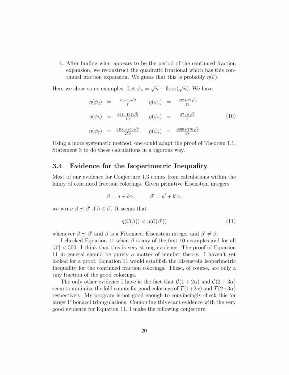
Here we show some examples. Let ψn =√n− floor(

√n). We have

η(ψ2) = 75+53√2

7η(ψ3) = 132+72

√3

13

η(ψ5) = 321+137√5

19η(ψ6) = 27+9

√6

2

η(ψ7) = 3100+856√7

259η(ψ8) = 1569+370

√8

98

(10)

Using a more systematic method, one could adapt the proof of Theorem 1.1,Statement 3 to do these calculations in a rigorous way.

3.4 Evidence for the Isoperimetric Inequality

Most of our evidence for Conjecture 1.3 comes from calculations within thefamiy of continued fraction colorings. Given primitive Eisenstein integers

β = a+ bα, β′ = a′ + b′α,

we write β β′ if b ≤ b′. It seems that

η(C(β)) < η(C(β′)) (11)

whenever β β′ and β is a Fibonacci Eisenstein integer and β′ 6= β.I checked Equation 11 when β is any of the first 10 examples and for all

|β′| < 500. I think that this is very strong evidence. The proof of Equation11 in general should be purely a matter of number theory. I haven’t yetlooked for a proof. Equation 11 would establish the Eisenstein IsoperimetricInequality for the continued fraction colorings. These, of course, are only atiny fraction of the good colorings.

The only other evidence I have is the fact that C(1 + 2α) and C(2 + 3α)seem to minimize the fold counts for good colorings of T (1+2α) and T (2+3α)respectively. My program is not good enough to convincingly check this forlarger Fibonacci triangulations. Combining this scant evidence with the verygood evidence for Equation 11, I make the following conjecture.

20

Conjecture 3.1 Suppose that β is a Fibonacci Eisenstein integer β β′.Let C = C(β). Let C ′ be an arbitrary good coloring of T (β′). Then we haveη(C) < η(C ′), with equality if and only if β′ = β and C ′ is equivalent to C upto symmetry and color-reversing.

This conjecture would combine with Equation 3 to prove Conjecture 1.3.It is worth pointing out that that the continued fraction colorings are

far from the best in many cases. Figure 9 compares the continued fractionC(1 + 5α) (left) with another coloring of T (1 + 5α) (right) which seems tobe the one which minimizes the fold count.

Figure 9: Two good colorings of T (1 + 5α).

The continued fraction coloring has fold count 43 and E.I.R. 29.822... Thepretty coloring on the right has fold count 35 and E.I.R. 19.758. What we aresaying is that the continued fraction colorings can often be improved, but the“Fibonacci colorings” are so good that they beat any of these improvements.

21

4 A Bound on the Isoperimetric Ratio

In this chapter we prove Theorem 1.2. We first establish an isoperimetricinequality for a special kind of polygon and then we give the main argument.

4.1 Special Hexagons

Say that a special hexagon is a convex hexagon whose interior angles are all2π/3. The regular hexagon is an example, and all other special hexagonsare obtained from the regular one by pushing the sides in and out parallelto themselves. Our first result is a version of the isoperimetric inequality forspecial polygons. This result is undoubtedly well-known.

Lemma 4.1 The length and area of a special hexagon satisfy the inequality

length2

area≥ 8√

3. (12)

Proof: it is an elementary exercise, and it is also discussed at length in [T],that the area of such a hexagon is a quadratic function of the side lengths`1, ..., `6. By symmetry, the desired function is symmetric in the arguments.Therefore, we have

area = a(`1 + ...+ `6)2 + b(`21 + ...+ `26).

Considering the unit regular hexagon and the unit equilateral triangle, whichis a limiting case, we get the relations

36a+ 6b =3√

3

2, 9a+ 3b =

√3

4.

Solving these equations leads to the formula

area =1

6√

3(`1 + ...+ `6)

2 − 1

4√

3(`21 + ...+ `26). (13)

If we hold the perimiter fixed, we maximize the area by minimizing the sumof the squares of the lengths. This happens when all lengths are equal, andthe ratio of interest is scale-invariant. Plugging in `1 = ... = `6 = 1 andcalculating, we get the advertised inequality. ♠

22

4.2 Eisenstein Polygons

We define an Eisenstein polygon to be a convex polygon whose sides are con-tained in the 1-skeleton of the unit equilateral triangulation. We consideredEisenstein trapezoids at length in §2. Such polygons have at most 6 sides,and up to scaling they are all limits of the special polygons just considered.Let f(P ) denote the perimeter of an Eisenstein polygon and let F (p) denotethe number of triangles it contains. As an immediate consequence of Lemma4.1, we have

f 2(P )

F (P )≥ 6. (14)

Now we relate Eisenstein polygons to good colorings. Let C be a goodcoloring of some triangulation T with degree sequence 6, ..., 6, 2, 2, 2. Ourgoal is to show that η(C) ≥ 3. Let f denote the fold count and let F be thenumber of faces.

Since T has some vertices where the degree is not divisible by 3, thecoloring C must use both black and white. Note that C partitions T into afinite number of monochrome regions with connected interior.

Lemma 4.2 Each monochrome region is isometric to an Eisenstein polygon.

Proof: To make the argument clearer, we shave off the outer ε of P , sothat its boundary is does not self-intersect. Let Pε be this slightly smallerpolygon. Since both colors occur at the triangles touching each degree 2vertex, we see that Pε does not contain any degree 2 vertices. Hence Pε islocally Eucidean. We study the boundary ∂Pε.

Each vertex vε of ∂Pε is eithin ε of a unique vertex v of P . Because Pcomes from a good coloring, v has at most 3 white triangles around it. Henceeach boundary component of Pε is locally convex: It always turns in the samedirection. This situation rules out the possibility that some component of∂Pε bounds P on one side and some othe (smaller) polygon on the other side.Such a boundary component would necessarily have a point which was notlocally convex. Informally, we say that Pε has no holes.

Since Pε is locally Euclidean and has no holes, Pε is either isometric to aconvex polygon or else Pε is not simply connected in the orbifold sense. Thisis to say that one of two things is true:

• The lift Pε of Pε to C contains an unbounded bi-infinite curve.

23

• The lift Pε contains a closed loop which surrounds a finite number oforder 3 symmetry points.

The first case combines with local convexity to show that there are 2 bound-ary components of Pε, both straight lines. But then Pε is a flat annulusbounded by geodesics. Such an annulus does not exist in the doubled equi-lateral triangle.

The second case directly contradicts local convexity. Pε would have aboundary component that was a closed loop bounding a polygon not con-tained in Pε. This gives the same contradiction as the “no holes” argument.

These contradictions show that in fact Pε is a convex polygon. Lettingε→ 0 we see that P is also a convex polygon. But then P is also an Eisen-stein polygon. ♠

4.3 The Main Argument

Let C be a good coloring as above. We can choose the colors so that thereare at least FW ≥ F/2 white triangles. Let P1, ..., Pk be the white connectedregions regions. We proved above that each Pj is an Eisenstein polygon. Letfj = f(Pj) and Fj = F (Pj). We have

minj

f 2j

Fj≥ 6. (15)

We also observe that each black-white interface in particular lies in theboundary of some Pj. Furthermore, the two boundaries ∂Pi and ∂Pj aredisjoint except perhaps for vertex intersections when i 6= j. These two ob-servations imply that f = f1 + ...+ fk. Hence

2f 2

F=

f 2

F/2≥ f 2

FW≥ f 2

1 + ...+ f 2k

FW=f 21

F1

⊕ ...⊕ f 2k

Fk≥ 6. (16)

Here ⊕ denotes the Farey sum: We add the numerators and we add thedenominators. As is well known, the Farey sum of some fractions lies betweenthe minimum and the maximum of the fractions. Stringing together theinequalities, we get f 2/F ≥ 3, as claimed. This completes the proof ofTheorem 1.2.

24

5 References

[T], W. P. Thurston, Shapes of Polyhedra, arXiv:math/9801088 (1998)

[W], D. B. West, Introduction to Graph Theory, 2nd Ed., Prentice-Hall(2000)

[Wo] S. Wolfram, Mathematica (2020) wolfram.com/mathematica.

25