Towards a numerical modeling of the couplingbetween RTM process and induced mechanicalproperties for rigid particle-�lled compositesAhmed El Moumen abdelghani saouab  ( abdelghani.saouab@univ-lehavre.fr )

Universite le Havre: Universite du HavreAbdellatif Imad Tou�k Kanit 

Research Article

Keywords: Resin Transfer Molding, Particle-�lled composite, Process/Properties coupling, Computationalhomogenization

Posted Date: September 9th, 2022

DOI: https://doi.org/10.21203/rs.3.rs-2007582/v1

License: This work is licensed under a Creative Commons Attribution 4.0 International License.  Read Full License

1

Towards a numerical modeling of the coupling between RTM process and

induced mechanical properties for rigid particle-filled composites

Ahmed El Moumen (a), Abdelghani Saouab (a)*, Abdellatif Imad (b), Toufik Kanit (b)

(a) Normandie Univ, UNIHAVRE, CNRS, LOMC, 76600 Le Havre, France

(b) Unite de Mecanique de Lille, Universite de Lille, Lille, France.

* abdelghani.saouab@univ-lehavre.fr

Abstract:

In this work, a method is proposed for modeling RTM process and the associated

mechanical behavior of composites filled with mono-sized spherical Alumina particles. This

method combines (i) a numerical model (RTM model) that allows the simulation of the RTM

process during the injection of particle filled resins, and (ii) a computational strategy of

mechanical properties based on the homogenization methods. These proposed models have

already been validated with experimental results. The RTM model is based on 3 sub-models:

the first one to describe the suspension flow, the second one to simulate the advance of the flow

front, and the last one to model the particles filtration by the fibrous medium. The distribution

result of the concentration of particles in the fibrous medium obtained at the end of the

simulation of the injection is used as input data for mechanical models of homogenization. The

homogenization numerical model was constructed from a representative volume element of the

microstructures using the Poisson process. The idea here is to couple these two steps (RTM

simulation + mechanical properties computation) in a complete model which allows at the same

time and in a single operation: to simulate the process of the manufactured composites loaded

with particles and to deduce their induced mechanical properties. The pertinence of the

proposed method is confirmed by the simulation of nine elastic properties of composites with

the finite element method. The influence of post-filling on the induced mechanical properties

has been studied.

Keywords: Resin Transfer Molding, Particle-filled composite, Process/Properties coupling,

Computational homogenization.

2

1. Introduction

Composite materials undergo continuous development in many industrial domains,

especially in the transport sector. Compared to other conventional materials, composite

materials have remarkable characteristics such as high specific strength, specific modulus and

lightness. These many features can be extended by adding new specific functionalities to the

composite materials by incorporating fillers (particles) into the material. These so-called

functional composites can achieve a wide range of new properties, such as thermal [1] and

electrical conductivity/insulation, magnetic or optical functionalities, and specific properties [2-

3] such as fire resistance, abrasion resistance, electromagnetic shielding and self-healing [4-5].

Their advantages also include the improvement of existing properties, such as weight savings

and amelioration of mechanical properties [6-7]. Tailored properties of composites are thus

obtained by adding fillers to the composite material during fabrication [8]. These properties

result from the physical characteristics of the particles, their volume ratio and their distribution

in the composite.

The incorporation of particles into composite materials can be achieved by two methods

[9-10], either by depositing inclusions on the surface of the preform (preform functionalization),

or by adding particles to the liquid resin and injecting the suspension obtained into the fibrous

medium (resin functionalization). In the last method, the liquid composite molding (LCM)

processes, are common techniques used for the fabrication of particle loaded composites. For

example, resin transfer molding (RTM) or vacuum assisted resin transfer molding (VARTM)

was used with a suspension to achieve certain properties in the composite, such as electrical

[11-12] and thermal conductivity [13-14] flame retardancy [15-18] self-healing properties [19],

enhancement of mechanical properties [20-21] and weight-saving [22-24]. However, in LCM

processes, the resin functionalization becomes more challenging as it affects the impregnation

of the fibrous medium by the suspension and induces three main issues: an increase in the

suspension viscosity, a filtration of particles by the fibrous medium and a non-homogeneous

particle distribution within the finished part [25-28]. This crucial issue of the elaboration of

functional composites by LCM processes comes from the complexity of particle addition to

their fibrous structures. Indeed, the filtration of particles is a complex phenomenon that depends

on several parameters related to the process and the different materials used. Therefore, the

control of particle infiltration necessarily requires a good understanding of the physics of the

3

process and the influence of these parameters on the final properties of the structure. Numerical

modeling of the process/properties coupling is an undeniable tool to help overcome this

difficulty. Indeed, the desired properties result from the final distribution of the particles within

the fibrous medium and this distribution is controlled by the process parameters involved.

Given the interest of the subject, and despite the complexity of studying suspension flow

through fibrous media, a number of modeling efforts have been conducted; such as the work of

Erdal et al [29], Lefevre et al [30], Qian et al [31], Abliz et al; [32] and da Costa [33], in which

macroscopic models governing the filtration problems have been introduced to model the

suspension flow in textile preforms. These models take into account the coupling between

filtration and flow and allow the prediction of the evolution of the particle concentration during

the impregnation of the fibrous medium. However, to our knowledge, apart from our study [1]

dedicated to the coupling between RTM process and electrical properties of a particle-

reinforced carbon-epoxy composite laminate, no numerical study on the process/properties

coupling during the elaboration of particle-filled composites has yet been presented.

The objective of this paper is to develop a global modeling approach, which simulates

both the fabrication of a particle-filled composite by RTM process and the prediction of its

induced mechanical properties. The method proposed combines (i) a numerical model (RTM

model) that allows the simulation of the RTM process during the injection of particle filled

resins, and (ii) computational homogenization methods of the mechanical properties of

composites using the out-put results of (i)-step. The RTM model [34-36] is proposed to describe

the coupling between the suspension flow and the particle filtration by the fibrous medium

during the RTM process. Then, the prediction of the mechanical properties is obtained by a

computational homogenization method based on RVE and finite element method (FEM) as

given in [37-40]. The idea here is to couple and assemble these two steps (RTM modeling +

computational homogenization) in a complete model, to simulate the final distribution of

particles in the fibrous medium at the process end, and to compute the induced mechanical

properties of the composite, especially: Young’s moduli E11, E22 and E33, shear moduli G12,

G13 and G23, and Poisson ratio Nu12, Nu13 and Nu23. In the following, a detailed presentation

with various validations of the RTM model and the methods used for the homogenization of

the mechanical properties is given. Then, different applications of the global modeling approach

which couples the process simulation and the mechanical calculation are proposed.

4

2. The strategy of coupling RTM model / mechanical properties

computation

During the RTM process, the injection of resins loaded with certain fillers such as

Alumina particles, leads to an improvement of the mechanical properties of the manufactured

composite. These induced properties are directly dependent on the final distribution of particle

concentrations in the fibrous medium, which in turn is linked to the process parameters used.

To describe this link between process and properties, we propose a coupling strategy between

the RTM model and the computation of mechanical properties. This approach also shows how

the process parameters can be used to control the mechanical properties of the composite.

Figure 1 presents a description of the general principle of this strategy. This figure was divided

into two parts: (i) the first part describing the RTM model (flow and filtration) coupled with a

second part (ii) representing the computational of mechanical properties of composites. The

coupling is formulated by introducing the simulation results of the process (i.e. the final

concentration distribution of the particles in the fibrous medium) as input data for the second

step of the mechanical properties homogenization.

In the study of process/property coupling, reducing the cost of computational time is an

important issue. It is essential to optimize the proposed models to simulate the process and

property computation.

In a previous work [26], we proposed an approach to model the RTM process with a particle

filled fluid. This approach uses a stokes-Darcy coupling to describe the suspension flow at the

mesoscopic scale and a "solid" model to model the mass dynamics of the particles and their

retention, based on the equations of motion of each particle. Considering the large number of

particles involved in the suspension during the injection, the use of this model in the framework

of this work of coupling Process/Properties will generate rather long calculation times. For this

reason, a modeling approach at the macroscopic scale much less greedy in calculation time will

be used.

5

Figure 1: Illustration of the coupling strategy between the RTM model and the

computation of mechanical properties.

6

3. Modeling of the RTM process

3.1. Governing Equations

On a macroscopic scale, the flow of a suspension (particles filled-resin) through a

fibrous medium can be described using Darcy's law, as follows [1] [34]: 𝑈 = − 𝑲µ

∇𝑃 (1)

Where 𝑈, 𝑲,µ and 𝑃 are the flow velocity, the permeability of the medium, the

suspension viscosity and the pressure, respectively. The mass conservation equation can be

expressed by the continuity equation given as: 𝑑𝑖𝑣 (𝑈) = 0 (2)

The combination of equations (1) and (2) leads to the governing equation of the pressure

field which drives the flow: 𝑑𝑖𝑣 (𝑲µ

∇𝑃) = 0 (3)

The particles presence in the fluid causes an increase in the suspension viscosity and the

suspension flow through the fibrous medium leads to particle filtration and consequently to a

reduction in the porosity and the permeability of the fibrous medium. During the impregnation,

two types of particles are distinguished: the trapped particles (or retained particles), with a

volume fraction, noted 𝜎hereafter, and the moving particles with a volume fraction noted 𝜀𝐶,

where 𝜀 is the porosity of the filter medium and 𝐶 is the concentration of particles. The volume

fractions of trapped and moving particles vary in the impregnated fibrous medium as a function

of time and space. Retention 𝜎 and porosity ε of the fibrous medium can be related by the

equation (4) [30]: 𝜀 = 𝜀0 − 𝜎 (4)

Where 𝜀0 is the initial filter porosity, corresponding to the fibrous medium porosity.

To model the dispersion of particles in the laminar flow through the fibrous media, an

approach based on the calculation of the concentration of particles 𝐶 is used. This approach is

based on the advection transport equation, which results from the mass equation for the particles

[10]. This model was expressed as follows: ∂(εC + 𝜎)∂t + ∇. (UC) = 0 (5)

7

Where the terms (𝛛(𝛆𝐂)𝛛𝐭 ) represent the variation rate of the concentration of the moving

particles, (𝛁. (𝐔𝐂)) the advection effect and (𝝏𝝈𝝏𝒕) the deposit effect.

During the impregnation of a fibrous medium, the retention phenomenon is modeled by

the following constitutive law [10]: 𝜕(𝜎)𝜕𝑡 = 𝑈𝐶𝛼(1 − 𝜎𝜎𝑢) (6)

Where 𝜎𝑢 is the maximum possible deposit of particles that can be filtered by the fibrous

medium, and 𝛼 is the filtration coefficient variable as a function of the permeability 𝐾 and the

porosity 𝜀. This equation describes the kinetics of the retention with a possible re-suspension

of the particles. It relates the variation of the particles retained and filtered to the volume flow

of the entering particles by the filtration coefficient α. In its second limb, the first term

corresponds to the particle retention which is proportional to the flow of suspended particles 𝑈𝐶 and the second term represents the rate of re-suspension of the particles.

According to Erdal [29], the filtration coefficient 𝛼 varies during the impregnation of

the fibrous medium. It can be modeled as a function of permeability 𝐾 and the porosity 𝜀, as

follows:

11

0

2/3

0

2/1

0

01

1a

K

K

(7)

Where 𝑎1 is the model constant and 𝛼0 is the initial filtration coefficient.

The permeability evolution of the filter medium (fibrous medium + particles) can be

modeled using the model presented in [28]. This relationship predicts the filter permeability as

a function of the changing porosity as: 𝐾 = 𝐾0 [( 𝜀𝜀0) ( 1 − 𝜀1 − 𝜀0)−2] (8)

During the injection of the suspension, the porosity ε was affected by the local deposit

particles via Eq. (4), which in turn affects the filter permeability via Eq. (8) and the filtration

coefficient via Eq. (7). The spatio-temporal variation of the suspension viscosity is directly

related to the concentration evolution of the particles. It can be predicted according to the

relation (9) [28]:

8

𝜇 = 𝜇0 (1 − 𝐶𝐴)−2

(9)

Where µ0is the viscosity of the neat resin and 𝐴 is an empirical constant obtained via

experimental data.

3.2. Flow front advancement

During impregnation, the fibrous medium saturation by the suspension can be described by

a function ∅ (Level set function). We can distinguish two zones: a completely saturated region

where∅ = 1 and a dry region where ∅ = 0. The interface between these two sub-domains is

defined by 0 < ∅ < 1.The computational domain corresponds to the region of the fibrous

medium saturated with the suspension. It has a mobile border, which varies during the

impregnation: the flow front. To determine its position during the injection, the level set method

is used [13]. The principle of this method consists in determining a “level set function” ∅ by

solving the transport equation (10) based on the advection of this function by the flow velocity

and the interface thickness: 𝜕∅𝜕𝑡 + 𝑈∇∅ = 𝛾∇(𝜐∇∅ − ∅(1 − ∅) ∇∅|∇∅|) (10)

Where γ is the reinitialization parameter used to control the instability of the flow and 𝜐 the

adjustable thickness of the interface. The position of the flow front is determined by tracking

the “level set function” with a value of 0.5 (see Figure 2).

Figure 2: Illustration of the level set function variation during RTM process.

3.3. RTM numerical computation

The presented model is used to simulate the injection of suspension in the RTM process.

At the initial time t=0, we impose at any point x of the fibrous medium, the particles

concentration 𝐶(𝑥, 0) = 0, the retention 𝜎(𝑥, 0) = 0, the pressure 𝑃(𝑥, 0) = 0 and the porosity 𝜀(𝑥, 0) = 𝜀0.

Impregnated zone ∅ = 1

1 1 0.1 0 0 0

dry zone ∅ = 0

1 1 0.4 0 0 0

1 1 0.6 0 0 0

1 1 0.3 0 0 0

1 1 0.2 0 0 0

Inje

ctio

n

Ven

t

9

As boundary conditions, we imposed at the inlet (𝑥 = 𝑥0) during the injection: 𝐶(𝑥0, 𝑡) = 𝐶𝑖, 𝑄(𝑥0, 𝑡) = 𝑄𝑖𝑛𝑗(𝑡) or 𝑃(𝑥0, 𝑡) = 𝑃𝑖𝑛𝑗(𝑡)and at the vent(𝑥 = 𝑥𝑒): 𝑃(𝑥𝑒 , 𝑡) = 0.

For the wall boundary, we applied a Dirichlet condition (impermeable wall). 𝐶𝑖 is the

concentration of initial fillers in the suspension, 𝑃𝑖𝑛𝑗is the injection pressure and 𝑄𝑖𝑛𝑗 is the

injection flow rate.

The various equations of the model were implemented in the commercial software

COMSOL Multiphysics 5.4, via the partial differential equations (PDE’s) package. The

equation system composed of Darcy’s law (1), governing equation of the pressure field (3), the

continuity equation for particles (5), and the filtration kinetic equation (6), is solved in order to

determine the flow unknowns: pressure 𝑃, velocity 𝑈, particle concentration 𝐶 and the retention 𝜎.

3.4. Validation of the RTM numerical model

The numerical model proposed in this study was validated by a comparison with

experimental results and the analytical model, during a linear injection, which induces a

unidirectional flow of the suspension through the fibrous medium. In the experimental case, the

injection is carried out at imposed pressure and in the analytical case; the injection is conducted

at imposed velocity. In the last case, if 𝑉0 denotes the injection velocity of the used suspension,

the front velocity is can be determined by: 𝑈𝑓 = 𝑉0𝜀0 (11)

Indeed; at the flow front the retention can be considered null [28], therefore; according

to equation (4), the front porosity is equal to the initial porosity 𝜀0 of the medium. Since 𝜀0 is

constant, the integration of the equation (11) makes it possible to determine the front position 𝑋𝑓 as a function of time: 𝑋𝑓 = 𝑉0𝜀0 𝑡 (12)

The used velocities for analytical modeling are 𝑉1=0.85 mm/s, 𝑉2=2𝑉1and 𝑉3=3𝑉1.Table 1 presents the properties of the materials used and the conditions of the two tests

considered in the experiment. In the first test, the suspension is constituted of epoxy resin and

spherical boehmite nano-particles with an average diameter of 104 µm and the reinforcement

is a quasi-unidirectional carbon- fiber textile. The injection experiments are carried out on a

permeability test rig, which allows the extraction of fluid samples during impregnation and the

observation of flow fronts. The injections are conducted at constant pressure of up to 3 bar. The

10

injected suspension is extracted at five locations between the inlet and the outlet every 5 cm.

Then, the concentration of particles in the extracted samples is measured by thermo-gravimetric

analysis on a TA Instrument TGA Q5000. In the second test, the suspension is prepared based

on polyester resin and spherical micro-beads having a diameter of 12 µm and synthetic PET

fibers felt is used as reinforcement. The experimental setup is composed of a rigid tooling (steel

half mold and thick PMMA top plate). The mold is fed at constant pressure using a pressure

bucket, equipped with a motorized mixer so as to maintain a homogeneous blend of the

suspension. The flow is monitored through the PMMA mold top plate that allows observations

and to record the front kinetics. After polymerization, samples are cut out from the composite

part at known locations. Samples are weighed, measured and burnt at high temperature (500

°C) so that filler content can be evaluated at any distance from the inlet.

Parameters Test 1 [32] Test 2 [30] 𝐶𝑖 : Initial fillers concentration (%𝑣𝑜𝑙) 5.0 40.5

µ0: Viscosity of neat resin (Pa. s) 0.04 0.20 𝐾0: Fiber permeability (*10-10) (m2) 0.85 4.92 𝑉𝑓: Fiber volume fraction (%) 50.0 18.7 𝛼 : Filtration coefficient (m-1) 0.2703 0.27 𝑎1: Model constant 1.0 1.0 𝑃𝑖𝑛𝑗 : Injection pressure (Pa) 1.105 2.105

Table 1: Parameters used in the simulation.

Figure 3 presents the comparison of the numerical results of the proposed model with

the experimental and analytical results. Figure 3 (a) describes the numerical and analytical

kinetics of the flow front in the case of the injection velocities 𝑉1, 𝑉2 and 𝑉3, while Figure 3 (b)

and Figure 3 (c) describe the front kinetic and the final distribution of the particle concentration

along the preform, respectively in the case of test 1 and test 2.

This comparison shows that the numerical results of the model are in good agreement

with the analytical and experimental results. These results show very similar trends and profiles,

especially in the analytical case, and a low relative error occurs in the experimental case: 4%

(test 1, front advancement), 2% (test 1, concentration prediction), 6 % (test 2, front

advancement), and 5% (test 2, concentration prediction).

11

(a) Front kinetic for different injection velocities (V1=0.85 mm/s, V2=2 V1, V3= 3V1)

(b) Validation with experimental data of [32]

(c) Validation with experimental data of [30]

Figure 3: Comparison and validation of the numerical model with: (a) analytical and (b,

c) experimental results.

3.5. Numerical results of RTM model

In this section, the numerical results of the RTM process simulation were presented and

discussed. For that, a linear injection of a suspension (resin epoxy + particles), through a

preform (UD glass fibers) of rectangular geometry, at imposed injection velocity 𝑉𝑖 was

12

considered. The injection threshold is placed on the entire left edge of the preform and the vent

is placed on the right one (see Figure 2). The preform has a rectangular geometry of length 𝐿 =

0.2 m and height ℎ = 0.01 m. The features of materials, parameters of the numerical model and

injection conditions considered are detailed in Table 2.

µ0: Viscosity of neat resin (Pa. s) 0.1 𝛼0 : Initial filtration coefficient (1/m) 1 𝐾0: Fiber permeability (m2) 2.10-10 𝜎𝑢 ∶ Ultimate specific deposit 0.5 𝑉𝑓 : Volume fraction of fiber (%) 50 𝑎1 ∶ Parameter model 1 𝑉𝑖 ∶ Injection velocity (mm/s) 1.7 𝐶𝑖 ∶ Initial fillers concentration (%vol). 20

Table 2: Physical properties of materials and parameters used for the numerical

simulation.

The injection of the suspension was controlled at different times. Figure 4 shows the

filling state at different times (10s, 20s, 30s and 58s). The fibrous medium saturation is

described by the level set function ∅. The completely saturated region where ∅ = 1 is

represented by the red color, and the dry region where ∅ = 0 is in blue. This figure shows also

an enlargement at the interface level between these two sub-domains where 0 <∅<1.It reveals

the capacity of the Level set method to describe this fine interface.

(a) t=10s

(b) t=20s

(c) t=30s

(d) t=58s

Figure 4: Fibrous medium saturation during suspension injection for different times:

(a) t=10s, (b) t=20s, (c) t=30s, (d) t=58s.

13

The kinetics of the flow front obtained during this simulation is discussed. As

expected, a linear profile is obtained and it is noted that the complete filling of the mold is

reached after 58.5s. Figure 5 describes the evolution of the pressure field, the concentration and

the retention of the particles during the impregnation.

(a) Pressure evolution

(b) Concentration and retention evolution

Figure 5: Evolution of the pressure, concentration and retention during injection:(a)

Pressure evolution and (b) concentration and retention evolution.

It is noted that the pressure curves (Figure 5 a) have a decreasing linear profile and the

slopes which increase continuously during the injection. This is due to the increase in the

pressure at the injection threshold, which from the value 0.1 bar at t=1s, reaches 3.6 bar at the

end of the injection. Figure 5b shows the curves of particle distribution and retention in the

saturated area of the preform, during the injection. These curves have a descending profile and

show a non-homogeneous distribution of moving or captured particles. At the end of the

impregnation, a high particle concentration, greater than 15%, was distributed along ¾ of the

preform length, followed by a sudden and high decrease in the distribution of the particles on

14

the rest of the preform. While a small quantity of particles is retained by the fibrous medium

and accumulates in the vicinity of the injection threshold (𝜎 = 1.5%).

Figure 6 shows the spatial variation of the viscosity, permeability and particle

concentration at the end of the impregnation. The concentration and the viscosity present a

similar decreasing profile and the permeability a rather increasing profile. These curves reflect

the influence of the particles on the modification of the behavior of the viscosity and the

permeability and therefore on the flow.

Figure 6: Concentration, viscosity and permeability profiles at the end of the

impregnation (at time 𝑇f =58𝑠) From the results of the simulation, it appears that the distribution of particles is non-

uniform through the medium when the mold was completely filled at t=58s. To improve the

distribution of particles, the impregnation will be continued after the mold filling and the

suspension was evacuated from the outside of the mold through its vent. Figure 7 shows the

effect of the injection time on the distribution of the particles. From this figure, it appears that

a clear amelioration is obtained in the particle distribution at t=70s, and a quasi-constant profile

was obtained for 80, 90 and 100s. The final concentration at the vent was 17.22% for t=90s

instead of 4.26% at t=58s. Figure 8 illustrates this amelioration for different injection times.

15

Figure 7: Evolution of the concentration after the total mold filling.

𝑇𝑓 = 58𝑠

𝑇𝑓 = 70𝑠

𝑇𝑓 = 80𝑠

𝑇𝑓 = 100𝑠

Figure 8: Evolution of the concentration for different injection times.

4. Computational homogenization of the mechanical properties

4.1. Description of the homogenization method

The multi-scale architecture of the studied composites is more complex. It consists of

three different phases: resin, mono-sized spheres and the unidirectional (UD) fibers. Actually,

there is no FE code can directly model such three phase’s architecture. The proposed method

16

in this section consists of using two-step homogenization methods. This method is depicted in

Figure 9.

Firstly, the mechanical behavior of the suspension (resin + mono-sized particles) is

homogenized as a separate composite phase (composite 1), and then the obtained results are

used as input data of the second step homogenization of composite 2 (composite 1 + UD fibers).

The first step of homogenization was performed with the help of the numerical and the

analytical models validated with experimental data and the second step of the homogenization

was performed with the analytical models.

Figure 9: Two step homogenization method used in this study.

Suppose that the composite (suspension + UD fibers) is subjected to a macroscopic

stress Σ and a macroscopic strain Ε. The objective of the homogenization is to determine the

effective stiffness tensor 𝐶 of the composite and the effective compliance tensor 𝑆 such that:

Σ = C: E and 𝐸 = 𝑆: Σ (13)

For these tensors, the macroscopic fields are related to the averaged value of the local

microscopic fields via the following equations:

17

σ(x) = B(x): Σ and 𝜀(x) = A(x): E (14)

Where σ(x) and ε(x) are the local stress and strain fields and A(x) and B(x) are the

strain and the stress localization tensor. The macroscopic fields are related to the local

microscopic fields as:

Σ = ⟨σ(x)⟩ and E = ⟨ε(x)⟩ (15)

For the case of two-phase composite (resin and particles), the localization tensors of

composites (A and B) are obtained as: ⟨A(x)⟩ = C1A1 + C2A2 and ⟨B(x)⟩ = C1B1 + C2B2 (16)

Where “j=1,2” denote the matrix and particles phase and Cj the concentration rate of

phases.

4.2. Generation of RVE composite 1

The first step of the homogenization method consists of identifying and generating the

numerical representative volume element (RVE) of the suspension. In principle, at each

concentration of the particles in the composite, a VER will be associated. This RVE will then

be discretized into cubic volume.

The technique used for generating the RVE for numerical homogenization computations

is described in this section. Generally, the random sequential adsorption (RSA) algorithm [41]

is the most used algorithm for generating random packing’s. An improved version of the RSA

algorithm was proposed in [42]. In this study, we will instead use the Poisson process. The

associated algorithm was proposed in detail in our previous works [43-44], and it can be used

for particles with ellipsoidal or cylindrical shapes.

At the beginning of the computation in this algorithm, the position of the first particle

in the suspension is randomly selected. Then, the position of the second particle is drawn and

the repulsion distance is checked between two neighboring particles. If there is overlapping

between the particles’ positions, the position of the second particle is drawn again until the

repulsion distance was respected. This process is repeated until the desired volume fraction of

particles. Table 4 present the used algorithm.

The particles are characterized by an orientation distribution function (ODF) that

provides the probability of a particle to be oriented along with the defined tensor. In a global

18

coordinate system OXYZ, the particle orientation is defined by its two Euler angles, 𝜃 and 𝛽 (Figure 10). For the particles, each one is characterized by its own unit orientation vector q,

defined by 𝜃 and 𝛽 as: q1 = cosθ q2 = sinθsinβ q3 = sinθcosβ

(17)

Figure 10: Two Euler angles θ∈ [0, π] and 𝛽 ∈[0,2π] of particles with respect to the global Cartesian coordinate system (O, X, Y, Z) and the local Cartesian coordinate system (O′, x1, x2, x3).

Main Algorithm

Input data: N, R1, R2, C0

Output: (a, b, c), r and q of all particles

1: define a RVE matrix with dimension LxLxL. Set a corner as the origin

Set one of the matrix corners as the origin

2: for i=1→ N do

For each generated particles I

3: Assign a random position vector 𝑟0𝑖 4: Assign a random quaternion vector 𝑞0𝑖

5: end for

6: initialize the actual volume fraction C(t=0) =0.

7: while C(t=0) < C0 do

8: Verify tc: Collision time between two ellipsoids

9: Verify ts: Collision time between particles and the cube faces

10: Compute ∆t = min (tc, ts) 11: for i=1 → N do

12: change de position: move the particle i from t to (t+∆t) 13: end for

14: if ∆t <= tc then

15: update the position and the vector

16: else if ∆t = ts then

19

17: create a periodic image of the concerned particle

18: end if

19: Compute the new volume fraction of particles: C(t+∆t) = 𝟏𝑳𝟑 ∑ 𝟒𝟑 𝝅(𝒂𝒕+∆𝐭𝒊 𝒃𝒕+∆𝐭𝒊 𝒄𝒕+∆𝐭𝒊 )𝑵𝒊=𝟏

20: end while

21: continue the computations by adding the particles and changing the position until 𝐶(𝑡+∆t) = 𝐶0

N: Number of particles, Ri: radius of particles, (a, b, c) output dimension data of particles,

Table 4: Pseudo-code for generating particles in the suspension.

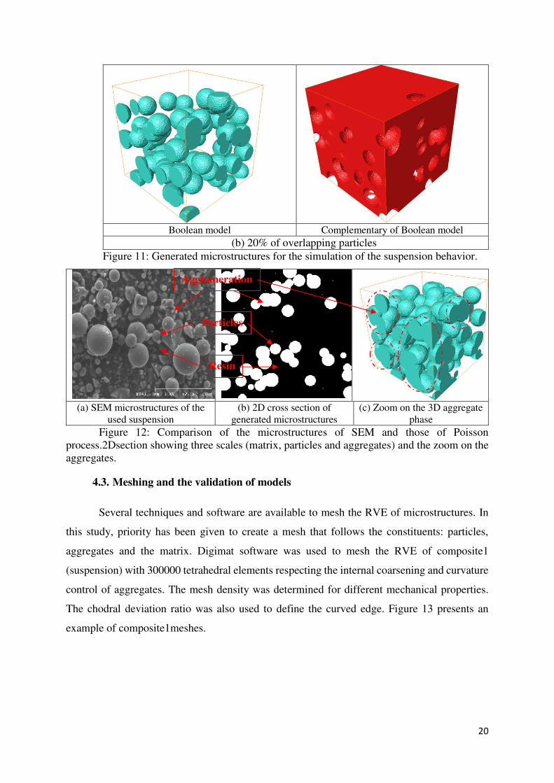
Figure 11 shows an example of random microstructures, generated using the Poisson

process, containing 200 spherical particles (radius R=100 µm) with a particle volume fraction

C0 of 20%. The hard model, presented in Figure 11a, was generated with a repulsion distance>

2R, and the Boolean model of Figure 11b was generated with the possibility of particles

overlapping. This last microstructure was considered in the calculations of the mechanical

properties of the suspension (resin + mono-sized particles) to model the agglomeration phase.

The complementary model of the hard and Boolean models, presented in Figure 11, corresponds

to the resin part in the VER.

The microstructure of the suspension was analyzed with the help of SEM microscopy.

Figure 12 shows the microscopic morphology of the suspension observed with SEM.

Qualitatively, this morphology illustrates that the microstructure contains three scales: the scale

of the resin, the scale of the aggregates and the scale of the particles. Looking at the

microstructure of Figures 12b and 12c, generated with the Poisson process, it seems that the

morphology contains the three scales as observed by SEM. A zoom-out in the aggregate phase,

obtained by overlapping particles, is presented in Figure 12c. The contact between particles and

the matrix was considered perfect without inter-phase.

Hard model Complementary of hard model

(a) 20% of non-overlapping particles

20

Boolean model Complementary of Boolean model

(b) 20% of overlapping particles

Figure 11: Generated microstructures for the simulation of the suspension behavior.

(a) SEM microstructures of the

used suspension

(b) 2D cross section of

generated microstructures

(c) Zoom on the 3D aggregate

phase

Figure 12: Comparison of the microstructures of SEM and those of Poisson

process.2Dsection showing three scales (matrix, particles and aggregates) and the zoom on the

aggregates.

4.3. Meshing and the validation of models

Several techniques and software are available to mesh the RVE of microstructures. In

this study, priority has been given to create a mesh that follows the constituents: particles,

aggregates and the matrix. Digimat software was used to mesh the RVE of composite1

(suspension) with 300000 tetrahedral elements respecting the internal coarsening and curvature

control of aggregates. The mesh density was determined for different mechanical properties.

The chodral deviation ratio was also used to define the curved edge. Figure 13 presents an

example of composite1meshes.

Agglomeration

Particles

Resin

21

Mesh of alumina particles Mesh of the composite 1

Figure 13: Example of meshes used in the simulation model.

For the computation of mechanical properties of composites, various analytical models

can be found in the literature. A list of these models adapted for the used suspension reinforced

with particles was presented by Al Habis et al. [45]. The popular existing approaches are: Mori

and Tanaka model [46] (MT), Hashin and Shtrikman bounds [47] (HS) and the generalized self-

consistent model [48] (GSC). These models allow to estimate the elastic properties of the

suspension.

The mathematical expressions for HS bounds are given as:

mmmi

m

HS

Gk

p

kk

pkk

43

)1(31

, and

iiim

i

HS

Gk

p

kk

pkk

43

31

1

(18)

)43(5

)2)(1(61

mmm

mm

mi

m

HS

GkG

Gkp

GG

pGG

, and

)43(5

)2(61

1

iii

ii

im

i

HS

GkG

Gkp

GG

pGG

(19)

Where ik , iG , mk and mG are the bulk and shear moduli for the particles i and matrix m

respectively and p the concentration of particles. The symbols + and – indicates the upper and

lower bounds of Hashin.

22

The expression of the MT model is given as:

)))(1(

)(1(

mim

mi

m

MT

kkpak

kkpkk

, wheremm

m

Gk

ka

43

3

)))(1(

)(1(

mim

mim

MT

GGpbG

GGpGG

, where )43(5

)2(6

mm

mm

Gk

Gkb

(20)

For the case of GCS, the expressions were proposed for shear and bulk moduli of the

suspension. For the suspension shear modulus, the estimated property is the solution of this

equation:

0)( 2 CG

GB

G

GA

m

GSC

m

GSC

(21)

Where the expressions of the coefficients A, B and C are specified in appendix A.

For the bulk modulus, the expression is:

mm

mi

mim

GSC

Gk

kkp

kkpkk

3

4)1(1

)(

(22)

The Young’s modulus of the suspension was computed using this equation:

Gk

kE

3

9

(23)

For the numerical model case, the simulation of a simple uni-axial test applied on the

suspension RVE is used to compute the Young’s modulus. The numerical results obtained are

presented in Table 4 and compared with experimental data and analytical results. From these

results, it appears that the experimental data and the numerical results are systematically

between the HS bounds (HS+ and HS-) and close to the MT model. The numerical model and

the analytical approaches were validated with the experimental data of [49].

HS- MT Numerical GSC Experimental

[49]

HS+

Young’s modulus (GPa) 1.412 1.9106 1.88 1.9368 2.48 ± 0.5 12.52

Table 4: Comparison of different results: numerical and analytical results vs

experimental data [49] of suspension with 20% of alumina particles.

Table 4 gives a comparison between mechanical properties obtained with different analytical,

experimental and numerical results for a suspension reinforced with a random distribution of

23

alumina particles. The detail of the experiment part and the mechanical properties of each

constituent were presented in [49].

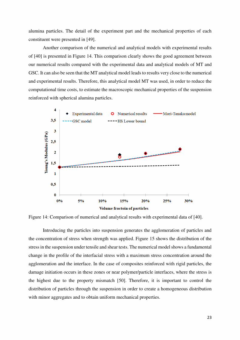
Another comparison of the numerical and analytical models with experimental results

of [40] is presented in Figure 14. This comparison clearly shows the good agreement between

our numerical results compared with the experimental data and analytical models of MT and

GSC. It can also be seen that the MT analytical model leads to results very close to the numerical

and experimental results. Therefore, this analytical model MT was used, in order to reduce the

computational time costs, to estimate the macroscopic mechanical properties of the suspension

reinforced with spherical alumina particles.

Figure 14: Comparison of numerical and analytical results with experimental data of [40].

Introducing the particles into suspension generates the agglomeration of particles and

the concentration of stress when strength was applied. Figure 15 shows the distribution of the

stress in the suspension under tensile and shear tests. The numerical model shows a fundamental

change in the profile of the interfacial stress with a maximum stress concentration around the

agglomeration and the interface. In the case of composites reinforced with rigid particles, the

damage initiation occurs in these zones or near polymer/particle interfaces, where the stress is

the highest due to the property mismatch [50]. Therefore, it is important to control the

distribution of particles through the suspension in order to create a homogeneous distribution

with minor aggregates and to obtain uniform mechanical properties.

24

Tensile deformation numerical test

Suspension Resin Particles

Shear deformation numerical test

Suspension Resin Particles

Figure 15: Stress concentration in the suspension reinforced with rigid particles under

tensile and shear tests. The red color shows the maximum stress

4.4. Mechanical behavior of UD fibrous media reinforced with rigid spheres

In this section, we focus on the modeling of the mechanical behavior of the suspension

and the composite in order to demonstrate the ability of the proposed approach to couple the

process parameters and the composite mechanical properties. For the computation of the

mechanical properties of the suspension, we recall that the epoxy resin and the alumina particles

used in this study have Young's modulus of 5 GPa and 500 GPa, respectively.

The simulations presented hereafter aim at evidencing the importance of taking into

account the effect of RTM process parameters on the mechanical properties of the composite.

To do this, a numerical study was conducted to analyze the effect of the addition of particles in

the composite and especially their distribution on the mechanical properties. The suspension

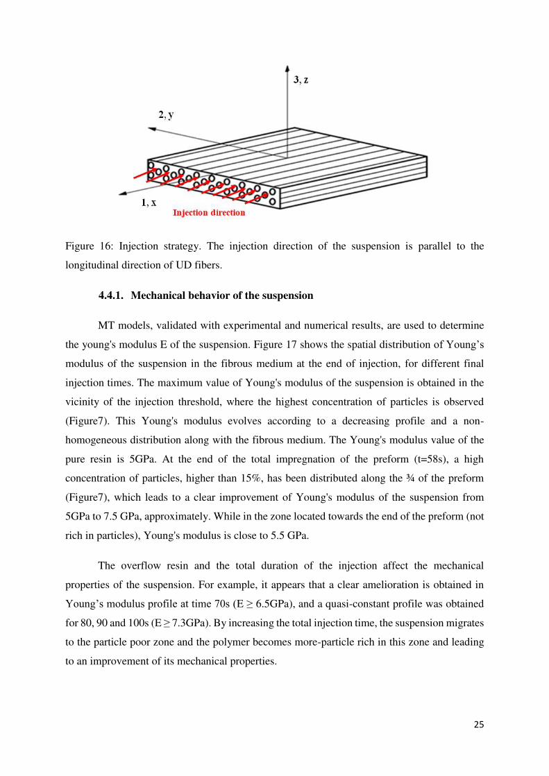
was injected in the direction of the longitudinal fibers, as presented in Figure 16.

25

Figure 16: Injection strategy. The injection direction of the suspension is parallel to the

longitudinal direction of UD fibers.

4.4.1. Mechanical behavior of the suspension

MT models, validated with experimental and numerical results, are used to determine

the young's modulus E of the suspension. Figure 17 shows the spatial distribution of Young’s

modulus of the suspension in the fibrous medium at the end of injection, for different final

injection times. The maximum value of Young's modulus of the suspension is obtained in the

vicinity of the injection threshold, where the highest concentration of particles is observed

(Figure7). This Young's modulus evolves according to a decreasing profile and a non-

homogeneous distribution along with the fibrous medium. The Young's modulus value of the

pure resin is 5GPa. At the end of the total impregnation of the preform (t=58s), a high

concentration of particles, higher than 15%, has been distributed along the ¾ of the preform

(Figure7), which leads to a clear improvement of Young's modulus of the suspension from

5GPa to 7.5 GPa, approximately. While in the zone located towards the end of the preform (not

rich in particles), Young's modulus is close to 5.5 GPa.

The overflow resin and the total duration of the injection affect the mechanical

properties of the suspension. For example, it appears that a clear amelioration is obtained in

Young’s modulus profile at time 70s (E ≥ 6.5GPa), and a quasi-constant profile was obtained

for 80, 90 and 100s (E ≥ 7.3GPa). By increasing the total injection time, the suspension migrates

to the particle poor zone and the polymer becomes more-particle rich in this zone and leading

to an improvement of its mechanical properties.

26

Figure 17: Spatial distribution of Young’s modulus of the suspension in the fibrous

media for different final injection times.

4.4.2. Mechanical behavior of the composite (UD fibers and the suspension)

In this second step of the homogenization, we are interested in the prediction of the

mechanical properties of the composite (UD + suspension), induced according to the different

total injection duration. These properties of the composite will be identified using the epoxy

Poisson ratio of 0.3 and Young's modulus of the suspension (calculated previously, see Figure

17), and those of the fibrous medium which are E=75 GPa for the Young’s modulus and 0.2 for

the Poisson ratio.

It should be noted that for the case of UD fibers reinforced with spherical particles,

Hashin and Rosen model [51] is considered as the most used approach to estimate the

mechanical properties of UD composites, namely the nine elastic moduli of the composite (three

principal Young’s moduli E11, E22, E33, three principal shear moduli G12, G13, G23 and

Poisson ratio Nu12, Nu13 and Nu23). In the first instance, this model was initially validated in

this study, with experimental data of Mbacke et al. [52] and the comparison was presented in

Table 5. A good estimation of the mechanical properties was obtained using this model.

Therefore, Hashin and Rosen model was subsequently used in this study.

E11 E22 G12 G23 Nu12 Nu23

Experimental data

[52]

45.0 12.0 4.5 - 0.3 -

Hashinand Rosen

model [51]

45.11 12.24 4.06 4.26 0.26 -

Table 5: Mechanical properties of 60% UD glass fibers composites: validation of the

analytical model with the experimental data.

27

The variation of the mechanical properties of glass fibers reinforced with the suspension

is determined as a function of the process parameters and presented in Figure 18. From this

figure, it appears that an important improvement of the transversal Young’s modulus (E22 and

E33) and the shear moduli (G12 and G23) was obtained compared with the case of C0=0%

(non-reinforcement). Results prove that the injection of particles through fibrous media leads

to improvement of the out-of-plane mechanical properties (E33 and G23 associated with Z-

direction) because the particle behavior is dominant compared with the X-direction where the

glass fibers behavior is dominant.

Longitudinal Young’s modulus E11 Transversal Young’s modulus E22=E33

Shear modulus G12=G13 Shear modulus G23

28

Poisson ration

Figure18: Mechanical behavior of UD composites initially reinforced with 20% of

rigid spheres for different total duration injections.

The evolution of mechanical properties of UD-composites was shown in Figure 18 for different

total duration injections. For example, the transversal Young’s moduli E22 and E33 of neat

composites are 10.5 GPa, and with the injection of particle for t=58 s, these moduli become

14.5 GPa. If the filtration continues for several times [58s, 100s], the particles migrate to the

other mold side (vent) which improves the mechanical properties of composites and keeps out

air. A direct correlation between mechanical properties and injection time was observed.

Therefore, a quasi-constant profile of mechanical properties was obtained for t=80, 90 and 100s.

No important modification in terms of the Poisson ratio and E11 was observed by injecting the

rigid particles through the UD fibers.

5. Conclusion

In this study, a complete model, which simulates the manufacturing of a particle-filled

composite by RTM process and the prediction of its induced mechanical properties has been

proposed. This global modeling approach combines (i) a numerical model which simulates the

injection of particle-filled resins during the RTM process and (ii) computational

homogenization methods of the mechanical properties of composites using the out-put results

of (i)-step. In this approach, the main idea is to take into account the process influence on the

induced mechanical properties of particle-filled composites. It has been formulated by a

process/properties coupling and obtained by the simultaneous simulation of the process and the

calculation of the mechanical properties induced by this process.

29

The numerical and analytical models proposed in this modeling approach have been

compared and validated with experimental results. Some obtained results have then been

presented to illustrate the capability of the proposed model. The pertinence of the proposed

method is confirmed by predicting the nine elastic moduli of the composite (E11, E22, E33,

G12, G13, G23, Nu12, Nu13, and Nu23) as a function of the particle concentration distribution

obtained at the injection end. More importantly, to describe the evolution of these moduli as a

function of the total injection duration. This last parameter proved to be crucial in the RTM

process, as it allows to better control of the final particle distribution and consequently, to

optimize the mechanical properties of the composite. The obtained results show that the

injection of the rigid particle through UD fibers by RTM process improves the out-of-plane

mechanical properties E22, E33, G12 and G23. For the case of the longitudinal Young’s

modulus E11, no important amelioration was observed.

Appendix A: constant for analytical model

3

5

23

7

3123

10

1 )1(252)2)1(63(2)54)(1(8 pG

Gp

G

Gp

G

GA

m

i

m

i

m

m

i

322

2 )107(4)8121)(1(50 mmm

m

i pG

G

3

5

23

7

3123

10

1 )1(504)2)1(63(4)51)(1(4 pG

Gp

G

Gp

G

GB

m

i

m

i

m

m

i

322 )715(3)3)(1(150 mmm

m

i pG

G

3

10

13

7

3123

10

1 )15)(1(252)2)1(63(2)75)(1(4 pG

Gp

G

Gp

G

GC m

m

i

m

i

m

m

i

322

2 )57()7)(1(25 mm

m

i pG

G

)2(35)2(35)5049)(1(1 mimi

m

imi

m

i

G

G

G

G

)107(4)57(2 ii

m

i

G

G

mm

m

i

G

G 57)108(3

Declaration

Funding

The authors declare that no funds, grants, or other support were received during the preparation of this

manuscript.

Conflict of interest/ Competing Interests

30

The authors declare no competing interests/ The authors have no relevant financial or non-financial

interests to disclose.

Code availability

Not applicable.

Availability of data and materials

The authors declare that the data and the materials of this study are available within the article.

Ethical approval

All procedures performed in studies involving human participants were in accordance with the ethical

standards of the institutional and/or national research committee and with the 1964 Helsinki

declaration and its later amendments or comparable ethical standards.

Consent to participate

Informed consent was obtained from all individual participants included in the study.

Consent to publish

The participants have consented to the submission of the case report to the journal.

Authors’ contributions A. El Moumen and A. Saouab: construct the idea. A. El Moumen: developed numerical model and

performed numerical simulation, analyzed data, draft manuscript preparation, and wrote the paper. A.

Saouab: analyzed results, analyzed numerical model, and co-wrote the paper. A. Imad and T. Kanit

discuss the results, correct the English and the paper format. All authors reviewed the results, prepared

the response to reviewer comments, and approved the final version of the manuscript.

References

[1] Djebara Y, Imad A, Saouab A, Kanit T. A numerical modelling for resin transfer molding

(RTM) process and effective thermal conductivity prediction of a particle–filled composite carbon–epoxy. J Compos Mater (2020); 55:3–15.

[2] Chohra M, Advani SG, Yarlagadda S. Filtration of particles through a single layer of dual

scale porous media. Adv Compos Lett (2007) 16:205–221

[3] Steggall-Murphy C, Simacek P, Advani SG, Yariagadda S, Walsh S. A model for

thermoplastic melt impregnation of fiber bundles during consolidation of powder- impregnated

continuous fiber composites. Composites Part A (2010) 41:93–100

[4] Nordlund M, Fernberg SP, Lundstrom TS. Particle deposition mechanisms during processing

of advanced composite mate rials. Compos Part A (2007) 38:2182–2193

[5] Tarfaoui M, El Moumen A, Boehle M, Shah O, Lafdi K. Self-heating and deicing epoxy/glass

fiber based carbon nanotubes buckypaper composite. J Mater Sci (2019) 54:1351–1362

[6] Shaker K, Nawab Y, Saouab A. Influence of silica fillers on failure modes of glass/vinyl ester

composites under different mechanical loadings. EngFract Mech (2019) 218:106605.

[7] Shaker K, Nawab Y, Saouab A. Experimental and numerical investigation of reduction in

shape distortion for angled composite parts. Int J Mater Form (2019) 11.https://doi.org/10.1007/s12289-

019- 01510-6

[8] Xie F, Pollet E, Halley PJ, Averous L. Starch-based nano-biocomposites. Prog Polym Sci

(2013) 38:1590–1628

31

[9] Manfredi E, Michaud V. Packing and permeability properties of E-glass fibre reinforcements

functionalised with capsules for self-healing applications. Compos. Part A Appl. Sci. Manuf. (2014) 66:

94-102.

[10] Louis BM, Maldonado J, Klunker F, Ermanni P. Particle distribution from in-plane resin

flow in a resin transfer molding process. Polym. Eng. Sci. (2019) 59: 22-34.

[11] Sandler JKW, Kirk JE, Kinloch IA, ShafferMSP, Windle AH. Ultra-Low Electrical

Percolation Threshold in Carbon-Nanotube-Epoxy Composites. Polymer (Guildf). (2003) 44: 5893–5899

[12] Andrianov IV,Danishevs'Kyy VV, Kalamkarov AL. Analysis of the effective conductivity

of composite materials in the entire range of volume fractions of inclusions up to the percolation

threshold. Compos. Part B Eng. (2010) 41: 503-507.

[13] Lee GW, Park M, Kim J, Lee JI, Yoon HG. Enhanced thermal conductivity of polymer

composites filled with hybrid filler. Compos. Part A Appl. Sci. Manuf. (2006) 37: 727-734.

[14] Qian L, Pang X, Zhou J, Yang J, Lin S, Hui D. Theoretical model and finite element

simulation on the effective thermal conductivity of particulate composite materials. Compos. Part B

Eng. (2017) 116 : 291-297.

[15] Guan FL, Gui CX, Zhang HB, Jiang ZG, Jiang Y, Yu ZZ. Enhanced thermal conductivity

and satisfactory flame retardancy of epoxy/alumina composites by combination with graphene

nanoplatelets and magnesium hydroxide. Compos. Part B Eng. (2016) 98: 134-140.

[16] Fernberg SP, Sandlund EJ, Lundstrom T. Mechanisms Controlling Particle Distribution in

Infusion Molded Composites. Journal of Reinforced Plastics and Composites. (2006) 25: 59-70.

[17] Wang YH, et al. Activated carbon spheres@NiCo2(CO3)1.5(OH)3 hybrid material modified

by ionic liquids and its effects on flame retardant and mechanical properties of PVC. Compos. Part B

Eng. (2019) 179: 107543.

[18] Kashiwagi T, Du F, Douglas JF, Winey KI, Harris RH, Shields JR. Nanoparticle networks

reduce the flammability of polymer nanocomposites. Nat. Mater. (2005) 4: 928-933.

[19] Mirzaei AH, Shokrieh MM. Simulation and measurement of the self-heating phenomenon

of carbon/epoxy laminated composites under fatigue loading. Composites Part B: Engineering (2021)

223: 109097

[20] Benyahia H, Tarfaoui M, Datsyuk V, El Moumen A, Trotsenko S, Reich S.Dynamic

properties of hybrid composite structures based multiwalled carbon nanotubes. Composites Science and

Technology (2017) 148: 70-79.

[21] Tarfaoui M, El Moumen A, Lafdi K, Hassoon OH, Nachtane M. Inter laminar failure

behavior in laminate carbon nanotubes-based polymer composites. Journal of Composite Materials

(2018) 52: 3655-3667.

[22] Tagliavia G, Porfiri M, Gupta N. Analysis of flexural properties of hollow-particle filled

composites. Compos. Part B Eng. (2010) 41: 86-93.

[23] Zhang X, et al. The effect of strain rate and filler volume fraction on the mechanical

properties of hollow glass microsphere modified polymer. Compos. Part B Eng. (2016) 101: 5363.

[24] Porfiri M, Gupta N. Effect of volume fraction and wall thickness on the elastic properties of

hollow particle filled composites. Compos. Part B Eng. (2009) 40: 166-173.

[25] Lefevre D, Comas-Cardona S, Binetruy C, Krawczak P. Modelling the flow of particle-filled

resin through a fibrous preform in liquid composite molding technologies. Compos. Part A Appl. Sci.

Manuf. (2007) 38: 2154-2163.

[26] Haji H, Saouab A, Nawab Y. Simulation of coupling filtration and flow in a dual scale

fibrous media. Compos. Part A Appl. Sci. Manuf. (2015) 76: 272-280.

[27] Nordlund M, Fernberg SP, Lundstrom ST. Particle deposition mechanisms during

processing of advanced composite materials. Compos. Part A Appl. Sci. Manuf. (2007) 38: 2182-2193.

[28] Sas HS, Erdal M. Modeling of particle–resin suspension impregnation in compression resin

transfer molding of particle-filled, continuous fiber reinforced composites. Heat Mass Transfer (2014)

50: 397-414.

[29] Erdal M, Guceri SI, Danforth SC. Impregnation molding of Particle-Filled preceramic

polymers: process modeling. J Am Ceram Soc (1999) 82: 2017–2028

32

[30] Lefevre D, Comas-Cardona S, Binetruy C, Krawczak P. Coupling filtration and flow during

liquid composite molding: Experimental investigation and simulation. Compos Sci Technol (2009) 69:

2127–2134.

[31] Qian E, Huang N, Lu J, Han Y. CFD–DEM simulation of the filtration performance for

fibrous media based on the mimic structure. Computers and Chemical Engineering (2014) 71: 478–488.

[32] Abliz D, Berg DC, Ziegmann G. Flow of quasi-spherical nanoparticles in liquid composite

molding processes. Part II: Modeling and simulation. Composites Part A (2019) 125: 105562.

[33] Reia da Costa EF, Skordos AA. Modelling flow and filtration in liquid composite moulding

of nanoparticle loaded thermosets, Composites Sciences and Technology (2012) 72: 799-805.

[34] El Moumen A, Saouab A, Siddig NA, Bizet L, Imad A. Numerical study to control the filler

distribution in fibrous media during the particle-filled resin transfer molding process. Int J Adv Manuf

Technol (2021) 114: 1669.

[35] Haji H, Saouab A, Park C H. Particles Deposit Formation and Filtering: Numerical

Simulation in the Suspension Flow Through a Dual Scale Fibrous Media.

MacromolecularSymposiaVolume (2014) 340: 44-51.

[36] Kang S, Lee H, Kim S, Chen D, Pui D. Modeling of fibrous filter media for ultrafine particle

filtration. Separation and Purification Technology (2019) 209: 461-469.

[37] El Moumen A, Kanit T, Imad A. Numerical evaluation of the representative volume element

for random composites. European Journal of Mechanics - A/Solids (2021) 86: 104181

[38] Sukiman MH, Kanit T, N'Guyen F, Imad A, El Moumen A, Erchiqui F. Effective thermal

and mechanical properties of randomly oriented short and long fiber composites.Mechanics of Materials

(2017) 107 : 56-70.

[39] El Moumen A, Tarfaoui M, Lafdi K. Computational Homogenization of Mechanical

Properties for Laminate Composites Reinforced with Thin Film Made of Carbon Nanotubes. Applied

Composite Materials volume (2018) 25: 569–588.

[40] El Moumen A, N'Guyen F, Kanit T, Imad A. Mechanical properties of poly–propylene

reinforced with Argan nut shell aggregates: Computational strategy based microstructures. Mechanics

of Materials (2020) 145: 103348.

[41] Rintoul MD, Torquato S. Reconstruction of the structure of dispersions, Journal of Colloid

and Interface Science (1997) 186: 467–476.

[42] Segurado J, Llorca J. A numerical approximation to the elastic properties of sphere-

reinforced composites, Journal of the Mechanics and Physics of Solids (2002) 50: 2107–2121.

[43] El Moumen A, Kanit T, Imad A, El Minor H. Effect of reinforcement shape on physical

properties and representative volume element of particles-reinforced composites: statistical and

numerical approaches. Mechanics of Materials (2015) 83: 1-16.

[44] El Moumen A, Kanit T, Imad A, El Minor H. Computational thermal conductivity in porous

materials using homogenization techniques: numerical and statistical approaches. Computational

Materials Science (2015) 97: 148-158.

[45] Al Habis N, El Moumen N, Tarfaoui M, Lafdi K. Mechanical properties of carbon

black/poly(e-caprolactone)-based tissue scaffolds. Arabian Journal of Chemistry (2020) 13: 3210-3217.

[46] Mori T, Tanaka K. Average stress in matrix and average elastic energy of materials with

misfitting inclusions. Acta Metall. (1973) 21: 571-574.

[47] Hashin Z, Shtrikman S. A variational approach to the theory of the elastic behaviour of

multiphase materials. J. Mech. Phys. Solids (1963) 11: 127-140.

[48] Christensen RM, Lo KH. Solutions for effective shear properties in three phase sphere and

cylinder models. J. Mech. Phys. Solids (1979) 27: 315-330.

[49] Al-Namie I, Ibrahim A, Hassan MF. Study the Mechanical Properties of Epoxy Resin

Reinforced With silica (quartz) and Alumina Particles. The Iraqi Journal For Mechanical And Material

Engineering (2011) 11: 486-506.

[50] Saoudi T, El Moumen A, Kanit T, Belouchrani MA, Benseddiq N, Imad A. Numerical

Evaluation of the Thermal Properties of UD-Fibers Reinforced Composites for Different Morphologies.

International Journal of Applied Mechanics (2020) 12: 2050032.

[51] Hashin Z, Rosen W. The elastic moduli of fiber reinforced materials. Journal

of applied mechanics (1964) 31: 223–232.

33

[52] M. Mbacke. Characterization and modeling of mechanical behavior of 3D braided

composites: Application to design of NGV tanks. (2014) HAL Id: pastel-00960667.

https://pastel.archives-ouvertes.fr/pastel-00960667