General rights Copyright and moral rights for the publications made accessible in the public portal are retained by the authors and/or other copyright owners and it is a condition of accessing publications that users recognise and abide by the legal requirements associated with these rights.

Users may download and print one copy of any publication from the public portal for the purpose of private study or research.

You may not further distribute the material or use it for any profit-making activity or commercial gain

You may freely distribute the URL identifying the publication in the public portal If you believe that this document breaches copyright please contact us providing details, and we will remove access to the work immediately and investigate your claim.

Downloaded from orbit.dtu.dk on: Jul 17, 2022

Toward Intelligent Inertial Frequency Participation of Wind Farms for the GridFrequency Control

Kheshti, Mostafa; Ding, Lei; Bao, Weiyu; Yin, Minghui; Wu, Qiuwei; Terzija, Vladimir

Published in:IEEE Transactions on Industrial Informatics

Link to article, DOI:10.1109/TII.2019.2924662

Publication date:2020

Document VersionPeer reviewed version

Link back to DTU Orbit

Citation (APA):Kheshti, M., Ding, L., Bao, W., Yin, M., Wu, Q., & Terzija, V. (2020). Toward Intelligent Inertial FrequencyParticipation of Wind Farms for the Grid Frequency Control. IEEE Transactions on Industrial Informatics, 16(11),6772 - 6786. https://doi.org/10.1109/TII.2019.2924662

1

Abstract—Evolving dynamics of modern power systems caused by high penetration of renewable energy sources increased the risk of failures and outages due to declining power system inertia. Large-scale wind farms must participate in frequency control that respond optimally in due time and adaptively in case of detecting power imbalance in the grid. Existing research studies have shown interest on stepwise inertial control (SIC) on wind turbines (WTs). However, the adequate power increment and time duration of WTs using SIC are the key questions that have not yet been fully addressed. This paper proposes an intelligent learning-based control system for wind turbines participation in frequency control, as well as for mitigating negative effects of the SIC. Firstly, an appropriate optimization model for grid frequency control is defined. Then, the model is solved using lightning flash algorithm (LFA), imperialist competitive algorithm and particle swarm optimization to control the WTs in a wind farm. The obtained dataset by LFA are applied to an artificial neural network that is trained with Levenberg-Marquardt algorithm and LFA. The proposed control system optimally adjusts the power increment and duration time of participation for each WT in the farm. Analyses on a 100 MW wind farm integrated into the IEEE 9-bus system and experimental tests proved the efficacy of the proposed approach.

Index Terms—Artificial neural networks, optimal frequency control, intelligent control, stepwise inertial control, wind farm.

I. INTRODUCTION

NTEGRATION of renewable energy sources into the power system gradually phases out the traditional power plants

M. Kheshti, L. Ding and W. Bao are with the Key Laboratory of Power

System Intelligent Dispatch and Control (Shandong University), Ministry of Education, Jinan, China (Emails: kheshti@ieee.org; dinglei@sdu.edu.cn).

V. Terzija is with the School of Electrical and Electronic Engineering, The University of Manchester, Manchester M139PL, UK.

Y. Hui is with the Nanjing University of Science and Technology, China. Qiuwei Wu is with the Center for Electric and Energy, Department of

Electrical Engineering, Technical University of Denmark, Lyngby 2800, Denmark, and the School of Electrical Engineering, Shandong University, Jinan 250061, China (Email: qw@elektro.dtu.dk).

This work was supported in part by the Project of Science and Technology of SGCC: Research on Coordinated Frequency Control for Power Grid with High Penetration of Renewable Energy. In part by the National Natural Science Foundation of China (51850410505), in part by the China Postdoctoral Science Foundation through grant (195346).

[1-4]. However, high penetration of intermittent renewable resources with limited storage capabilities decreases the system inertia and jeopardizes the grid frequency stability [5]. A grid with large scale of non-synchronous generation penetration and low inertia is very vulnerable to the faults and disturbances that may cause under frequency trips, cascade failures and outages.

Variable speed wind turbines (WTs), classified in type-3 and 4, e.g., doubly fed induction generators (DFIGs) and fully rated converter-based WTs are asynchronously connected to the grid via fast control power electronic converters. DFIGs as type-3 WT generators are the most common types and they are more efficient in power extraction than other types. They generally operate in the maximum power point tracking modes (MPPT) [6]. MPPT operation causes decoupling between the WTs and grid frequency so that they do not react to the frequency excursions. Early research showed that the WTs are capable of frequency participation using inertial control strategies [7-9].

The research on frequency participation of WTs is still in its early stages, since their inertial response is different from conventional power plants with more complicated control mechanism. The new grid codes request that wind farms must contribute to power system frequency control [10]. Upon occurring an active power imbalance in the grid, they can participate in grid frequency control using stepwise inertial control (SIC), in which WTs quickly increase their output powers and remain at over-production stage for a period of time [11-14]. The two very important questions arise therefore: i. How much active power do the spinning WTs need to

participate in frequency control? ii. For how long each WT needs to participate in frequency

control? Although the transmission system operators have stipulated

new grid codes, these two key questions have not been addressed for SIC schemes. In the SIC scheme, when a large frequency deviation occurs, output power of a WT should instantly increase which is followed by decrease of its rotor speed. To recover the rotor speed, the WT output power should only operate in the over-production mode within a limited time. The SIC over-production should then terminate to boost the rotor speed recovery. This termination event will cause a secondary frequency drop in the grid that may even worsen the system frequency excursion if adequate active power within a suitable time period has not been properly considered.

A proper control method needs to be developed to determine

Toward Intelligent Inertial Frequency Participation of Wind Farms for the Grid

Frequency Control Mostafa Kheshti, Member, IEEE, Lei Ding, Member, IEEE, Weiyu Bao, Minghui Yin, Qiuwei Wu,

Senior Member, IEEE, Vladimir Terzija, Fellow, IEEE

I

2

how much power increment a WT should produce in a wind farm and for how long it should operate in different situations. The current research studies in the literature have not explicitly addressed these problems. Also, the majority of these studies are only on one single WT, while very few studies consider wind farm frequency control [15-18].

Performance of classical control methods on power and frequency control is limited by the highly non-linear characteristics of WTs [19,20] and the grid [21,22]. Instead, evolutionary computation methods can be developed to solve such complex problems [23,24]. Application of such methods on several power system problems have been studied [25-28].

Motivated by the above mentioned problems and research potentials, this paper is dealing with optimum frequency participation of wind farms using an intelligent-based control method. The main contributions of the paper are as follows:

1) Using the system frequency response analysis, power system frequency control is modeled as a function of WTs frequency participation. The proposed model incorporates power increment and duration time of a WT as an optimization function subject to the practical constraints.

2) The proposed model is solved using metaheuristic methods, e.g., Lightning Flash Algorithm (LFA) [29, 30], particle swarm optimization (PSO) [31] and Imperialist Competitive Algorithm (ICA) [32]. LFA shows a robust performance against different scenarios as it has the advantages of both swarm-based and evolutionary-based algorithms and the results confirm its desired functionality to handle the complex dynamical problems. As the practical implementation of LFA or other evolutionary methods may require longer computation time in presence of disturbances, the obtained accurate data package from LFA is sent to an artificial neural network (ANN) for training.

(3) The SIC process is transformed into a Levenberg-Marquardt based and LFA based neural network to control the frequency participation of the wind farms in different uncertain conditions. The ANN is trained using the obtained data from LFA. The proposed control is tested and validated on the Western System Coordinating Council 9-bus test system and the experimental tests. The results demonstrate the effectiveness of the proposed method for wind farm frequency participation and provide important conclusions.

A brief outline of the paper is as follows. Section II presents the wind farm and SIC scheme. Frequency control from optimization perspective is presented in section III. Section IV contains the development of LFA and ANN on solving wind farm frequency control. Section V contains the simulation results on IEEE 9-bus system with a large-scale integrated wind farm and also the experimental tests on a wind integrated grid. The conclusion is drawn in section VI.

II. INERTIAL CONTROL CONCEPT

A. Wind farm principles

A wind farm is a group of inverter connected WTs to generate electricity from the wind. The total generated electric power of the wind farm is sum of the operating WTs,

,1

n

e i WFi

P P

(1)

where Pe,i and PWF are the output power of the i-th WT and the total output power of the wind farm, respectively; n is the total number of WTs in the wind farm. The electric power output of each WT generator is converted from the extracted mechanical power,

2 3, , ,(

1),

2m i i p i i i w iCP r v (2)

where ρ is the air density; i is the index number of WT, ri is the radius of i-th WT blades; vw,i is the wind speed flowing to the i-th WT. The blowing wind in the wind farm is considered as a vector containing different actual wind speeds on the site, hitting the WTs blades as v=[vw,1,…, vw,n]. The aerodynamic performance Cp,i of a WT is presented as follows [37]:

1 5

,

2.116

, 0.22 0.4 5 wii i i

wip iC e

(3)

where it depends on the tip-peed ratio λi and the pitch angle βi.

1

3

1 0.035

0.08 1wii i i

(4)

,

,

i r ii

w i

r

v

(5)

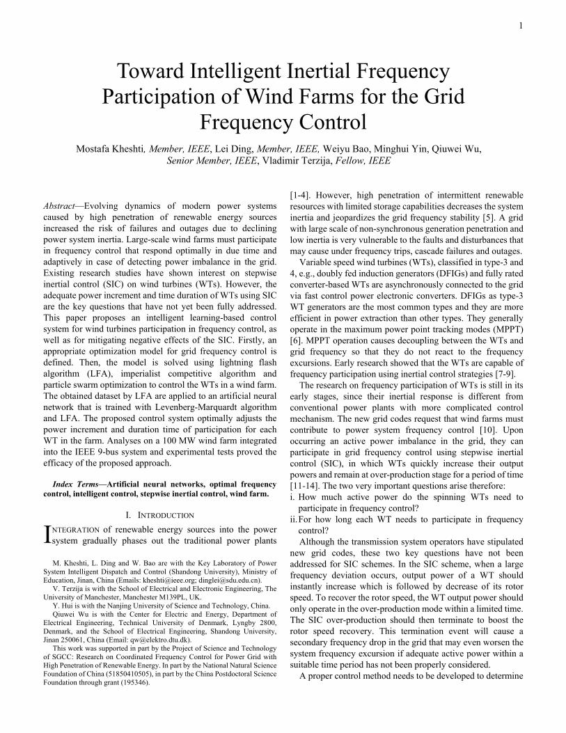
where ωr,i is the rotor speed of the i-th WT. The maximum aerodynamic performance Cp,i(λi,βi) of the WT appears when βi=0 as shown in Fig. 1. At an operative pitch angle, there exists an optimal value of rotor speed under a given wind speed.

(a) (b)

Fig. 1. Aerodynamic performance of a WT (a) as a function of λi and βi (b) as a function of vw,i and ωr,i when βi=0.

Under normal operations, the spinning WTs operate with maximum performance on MPPT mode with the output power:

,3

,( )r i optMP rPT iP k (6)

where kopt is the coefficient of MPPT curve of the turbine.

B. SIC principles

Upon occurrence of a power imbalance such as abrupt load demand or loss of generation, the power system frequency drops. A renewable connected grid has low inertia in which severe frequency drop may cause trip of under frequency relays, cascade failures or even blackouts if not controlled immediately. The frequency excursion can be arrested if the connected wind farms participate in frequency control. To do that, the wind farm should step up its output power and remain in over-production stage for a limited time to compensate the power imbalance in the grid. Then, it should terminate to initiate recovery process of the rotor speed. The inertia response of WTs is naturally energy neutral. It means that the period of over-production is followed by a power decay and lastly a recovery process to return back to its equilibrium. These

3

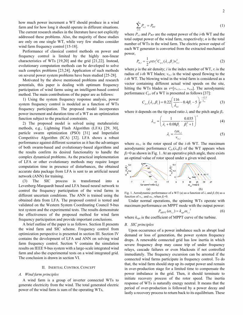
stages are shown in Fig. 2 and expressed as follows: A-B: the WT is working with its nominal rotor speed (ω0) and electric power output P0. Upon observing a power imbalance in the grid, its output power increases with a step-up power increment value of ΔPf. B-C: the WT remains in over-production stage with output of P0+ΔPf to compensate the power imbalance. However, as the output power is larger than the mechanical input, the rotor speed decreases. The process must terminate before over-deceleration to avoid the consequent rotor stall event. The SIC terminates at the termination time of toff. The rotor speed at this time is off. C-D: output power falls with the magnitude of ΔPoff and it is switched to the MPPT mode. This termination causes an adverse power imbalance in the system that imposes a secondary frequency drop in the grid. This secondary frequency drop may even have a larger frequency nadir if proper precautions on power increment (ΔPf) and an adequate termination time (toff) of SIC have not been applied. D-A: The rotor speed recovers along the MPPT trajectory to accelerate from off to the normal working point 0 in a time range of toff to tend.

(a)

Timetoff

Over-production stage Recovery stage

t0

ΔPoff

output power of WT

A

B C

D

(b)

ΔPf

P0

ωoff ω0 ω0

Pr(t)

A

PMPPT

ANN

SIC

Pe RSCcontroller

(c) Fig. 2. SIC process of a WT in the wind farm.

C. SIC formulation Proper inertial control of a wind farm requires understanding

of properties of each wind turbine parameters such as rotor speed, power increment contribution and duration of their participations. The following equations can describe the inertial control properties of i-th WT in a wind farm when a power imbalance occurs at t0=0.

The step-up power increment (A-B) can be defined using swing equation,

, ,, ,

d

d2 r

i i em iw r iPHt

P

(7)

where Hw,i refers to the wind turbine inertial constant.

, ,,m i e iP P are the mechanical input and the electric power

output of the WT, respectively. Integration of the swing equation during over-production stage (B-C) determines the termination time and the rotor speed, where the electric power output is 0, ,i f iP P .

,

0

,

,

, ,

, 0,0

, ,(

2 d d

)

off i

i

off iw i r ir

m i i f

t

off ii

Ht

P PPt

(8)

Solving this complex nonlinear integration can be achieved using Riemann Sum:

,, 0, ,0

1 , ,,

,

,

0

lim [ , ]2

;( ) ( )k

Nr i k

k r i k i off ik m r i k i f i

w ioff iP

Ht

P P

(9)

Obtaining the rotor speed off,i at the termination time leads to obtaining the power drop of WT at the termination (C-D):

0, ,

0, ,

, ,

3,

( )off i ofi f i MPPT

i f

f i

opt offi i

P P P P

P P k

(10)

The recovery stage (D-A) of the turbine follows the MPPT trajectory in which we have:

, ,3

, ( ) ( )MPPTr i r i opt r iP t P k (11)

Instead of dealing with the cubic recovery function shown in (D-A), a rather piecewise function can be used as shown in Fig. 2(b). This simplification effectively mitigates the computation time when considering numerous WTs in a wind farm. Also, it has a negligible effect on the amplitude of secondary frequency nadir and the termination time. Another advantage is that by using the real cubic function (D-A), when the rotor speed approaches the working point A, the denominator in (8) will be very small and the integration goes to a very high value. Therefore, the Riemann Sum with the piecewise function avoids such miscalculation.

0, , ,

,

, , , ,

,

0,

( ),( ) offi f i off i r i off ii end i

end i

r i

i

P P P k t t t t tP t

P t t

(12)

where kr,i is the slope of the piecewise function at offt t . At

this time, the WT rotor speed is ,off i and it is working in the

MPPT mode,

2, ,3

t toffoff

MPPT MPPT r rr i opt off i

r t t

P P d dk k

t dt dt

(13)

Using (7) we have,

, , ,

, ,

( )

2off

m i off i off ir

t t w i off i

d

d

P P

Ht

(14)

Substituting (14) into (13), kr,i is obtained,

,,

,, , ,( )

32

m i ofr i opt

f i off ioff i

w i

P Pk k

H

(15)

The rotor speed of turbine i, ,off i at the termination time is

calculated as follows:

0, ,

3, 0,

, ,3

,,

3

( ) 2opt

off i ioff i off i w i

off iop t

i

o

i

t p

fk Pt P

P t H

k k

(16)

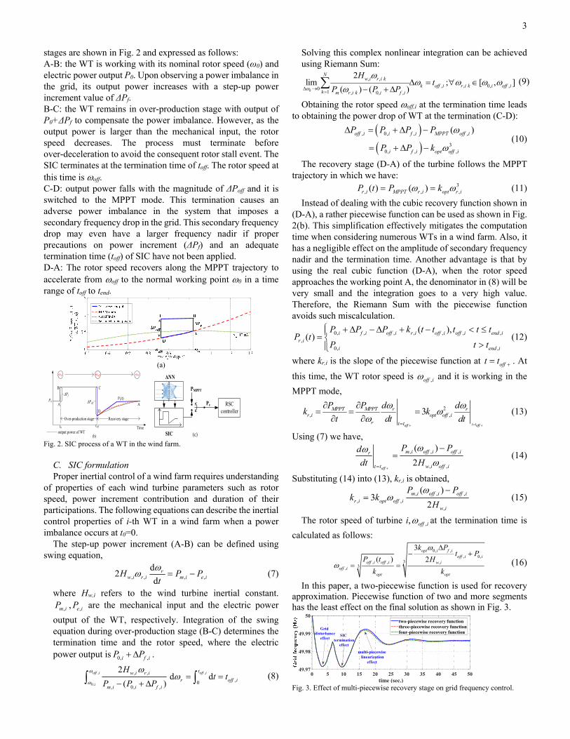
In this paper, a two-piecewise function is used for recovery approximation. Piecewise function of two and more segments has the least effect on the final solution as shown in Fig. 3.

0 5 10 15 20 25 30 35 40 45 50time (sec.)

49.97

49.98

49.99

50two-piecewise recovery functionthree-piecewise recovery functionfour-piecewise recovery function

Griddisturbance

effectSIC

terminationeffect

multi-piecewiselinearization

effect

Fig. 3. Effect of multi-piecewise recovery stage on grid frequency control.

4

III. OPTIMIZATION MODELING

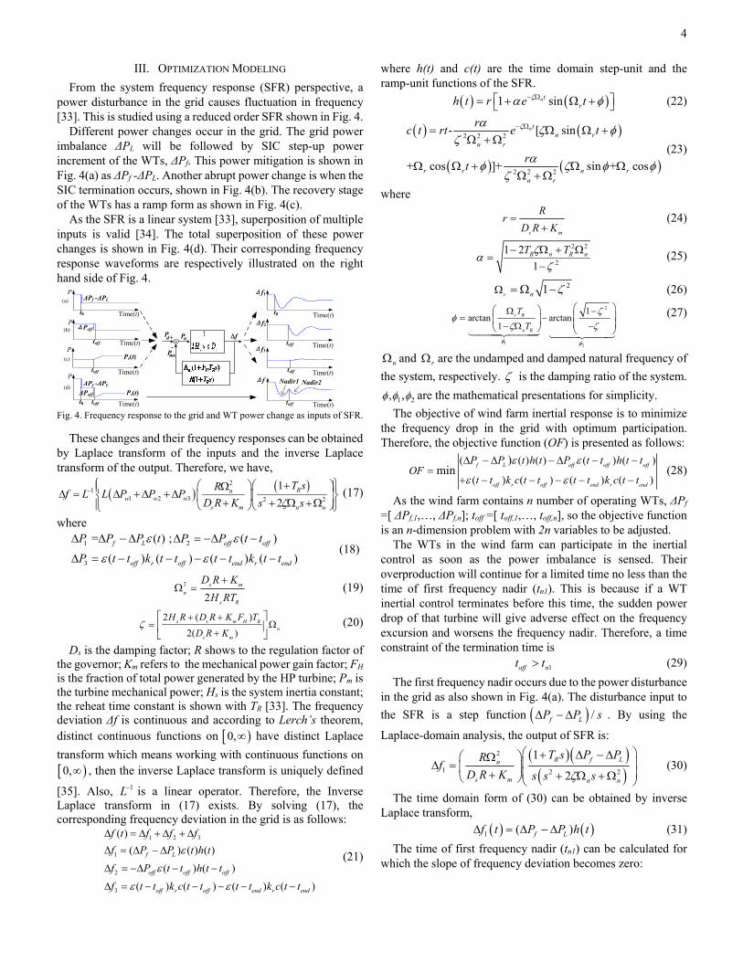
From the system frequency response (SFR) perspective, a power disturbance in the grid causes fluctuation in frequency [33]. This is studied using a reduced order SFR shown in Fig. 4.

Different power changes occur in the grid. The grid power imbalance ΔPL will be followed by SIC step-up power increment of the WTs, ΔPf. This power mitigation is shown in Fig. 4(a) as ΔPf -ΔPL. Another abrupt power change is when the SIC termination occurs, shown in Fig. 4(b). The recovery stage of the WTs has a ramp form as shown in Fig. 4(c).

As the SFR is a linear system [33], superposition of multiple inputs is valid [34]. The total superposition of these power changes is shown in Fig. 4(d). Their corresponding frequency response waveforms are respectively illustrated on the right hand side of Fig. 4.

+

-

dP aP

msP

f

P Δf1

Δf2

Δf3

Δf

(a)

(b)

(c)

(d)

t0

toff toff

toff toff

toff

t0

ΔPf -ΔPL

ΔPoff

Nadir1 Nadir2

t0 toff

ΔPf -ΔPL

ΔPoff Pr(t)

Time(t)

Pr(t)

P

P

P

Time(t)

Time(t)

Time(t)

Time(t)

Time(t)

Time(t)

Time(t) Fig. 4. Frequency response to the grid and WT power change as inputs of SFR.

These changes and their frequency responses can be obtained by Laplace transform of the inputs and the inverse Laplace transform of the output. Therefore, we have,

21

1 2 3 2 2

1

2Rn

w w ws m n n

T sRf L L P P P

D R K s s

(17)

where

2

3

1 = ( ) ; ( )

( ) ( ) ( ) ( )

f off off

off

L

r off end r end

t t t

t t k t t t t k t

P P P

P t

P P

(18)

2

2 s

n

s m

R

D R K

H RT

(19)

2 ( )

2( )s s m H R

m

n

s

H R D R K T

D R

F

K

(20)

Ds is the damping factor; R shows to the regulation factor of the governor; Km refers to the mechanical power gain factor; FH is the fraction of total power generated by the HP turbine; Pm is the turbine mechanical power; Hs is the system inertia constant; the reheat time constant is shown with TR [33]. The frequency deviation Δf is continuous and according to Lerch’s theorem, distinct continuous functions on 0, have distinct Laplace

transform which means working with continuous functions on

0, , then the inverse Laplace transform is uniquely defined

[35]. Also, 1L is a linear operator. Therefore, the Inverse Laplace transform in (17) exists. By solving (17), the corresponding frequency deviation in the grid is as follows:

1 2 3

1

2

3

( )

) ( ) ( )

( ) ( )

( ) ( (

(

) ( ) )

off off

off r off end r end

f L

off

t

t h t

P t t h t t

f f f

t t k c t t t t k

f

f P P

c t t

f

f

(21)

where h(t) and c(t) are the time domain step-unit and the ramp-unit functions of the SFR.

1 sinntrh t r e t (22)

2 2

2 2

2

2

- [ sin

+ cos ]+ sin + cos

ntr

r

r

n

r nn r

n

r

rc t rt e t

rt

(23)

where

s m

Rr

D R K

(24)

2 2

2

1 2

1R n R nT T

(25)

21r n (26)

1 2

21arctan arctan

1r R

n R

T

T

(27)

n and r are the undamped and damped natural frequency of

the system, respectively. is the damping ratio of the system.

1 2, , are the mathematical presentations for simplicity.

The objective of wind farm inertial response is to minimize the frequency drop in the grid with optimum participation. Therefore, the objective function (OF) is presented as follows:

( ) ( ) ( ) ( )

( ) (

(

) ( ) ( )

)min

L off off

off r off end r en

f off

d

t h t P t t h t tOF

t t k c t t t t t t

P

k c

P

(28)

As the wind farm contains n number of operating WTs, ΔPf =[ ΔPf,1,…, ΔPf,n]; toff =[ toff,1,…, toff,n], so the objective function is an n-dimension problem with 2n variables to be adjusted.

The WTs in the wind farm can participate in the inertial control as soon as the power imbalance is sensed. Their overproduction will continue for a limited time no less than the time of first frequency nadir (tn1). This is because if a WT inertial control terminates before this time, the sudden power drop of that turbine will give adverse effect on the frequency excursion and worsens the frequency nadir. Therefore, a time constraint of the termination time is

1off nt t (29)

The first frequency nadir occurs due to the power disturbance in the grid as also shown in Fig. 4(a). The disturbance input to

the SFR is a step function /f LP P s . By using the

Laplace-domain analysis, the output of SFR is:

2

2 21

1

2

R f Ln

s m n n

T s P Pf

R

D R K s s s

(30)

The time domain form of (30) can be obtained by inverse Laplace transform,

1 ( )f Lf t P P h t (31)

The time of first frequency nadir (tn1) can be calculated for which the slope of frequency deviation becomes zero:

5

11sin 0n

n f L tr

s m

R P Pe t

D Rt K

d f

d

(32)

To satisfy (32), 1rt n . Substituting 1 from (27)

into (32), the time when tn1 occurs is as follows:

11

1tan

1r R

nn

r R

T Rt

T R

(33)

The time of first frequency nadir is only a function of power system parameters and it occurs at the same time for all disturbances. tn1 is independent of magnitude of disturbances.

Also, the rotor speed decelerates during frequency participation. When the rotor speed goes less than its threshold, the mechanical turbine stalling occurs and it is disconnected from the grid. The sudden stall is a power loss with serious frequency deviation. To avoid mechanical rotor stall, the SIC should terminate before speed drops less than the threshold. The operating rotor speed range for DIFG WTs is usually between 0.7 and 1.2 pu.

min( , )foff offtP (34)

Mandatory frequency response in grid codes like that of U.K. is needed to maintain the frequency within statutory (49.5Hz - 50.5Hz) and operational limits (49.8Hz-50.2Hz) [10,13,38-39]. The magnitude of frequency drop should not be larger than an acceptable margin, otherwise the under-frequency load shading operates. Therefore, the SIC process must result in a better frequency response than the cases without WTs participations.

min( ) max( , 0.5), ,f offf Pt ft (35)

The formulated practical constraints in (29), (34) and (35) are applied on the objective function (28).

IV. CONTROL METHOD

Considering different locations, geographic of the wind farm, types of turbines and wind direction, each WT may have a different wind speed, hence producing different powers. The objective is to adjust the best magnitudes of power increments and the duration of the inertial control action on each WT to minimize the frequency drop in the grid.

Due to the large curse of dimensionality and complexity of the problems, application of classical methods may not be feasible. Instead, evolutionary computation is required to analyze the collected data of the farm and set the best adjustments on each WT to arrest the frequency deviation.

The question is that when a power imbalance occurs, how much power each turbine should overproduce and for how long they should operate to minimize the frequency drop, all subject to the practical intermittencies and constraints. This paper uses an intelligent learning-based system to solve this problem and ensure high efficiency of large-scale wind farm participation in the grid frequency control.

ANNs are very efficient in solving the nonlinear and complex problems which are difficult to solve by conventional methods. ANNs require abundant and reliable input-output data to be trained and provide an intelligent learning-based control. LFA is applied on the modeled objective function for different scenarios subject to the practical constraints. The solution of

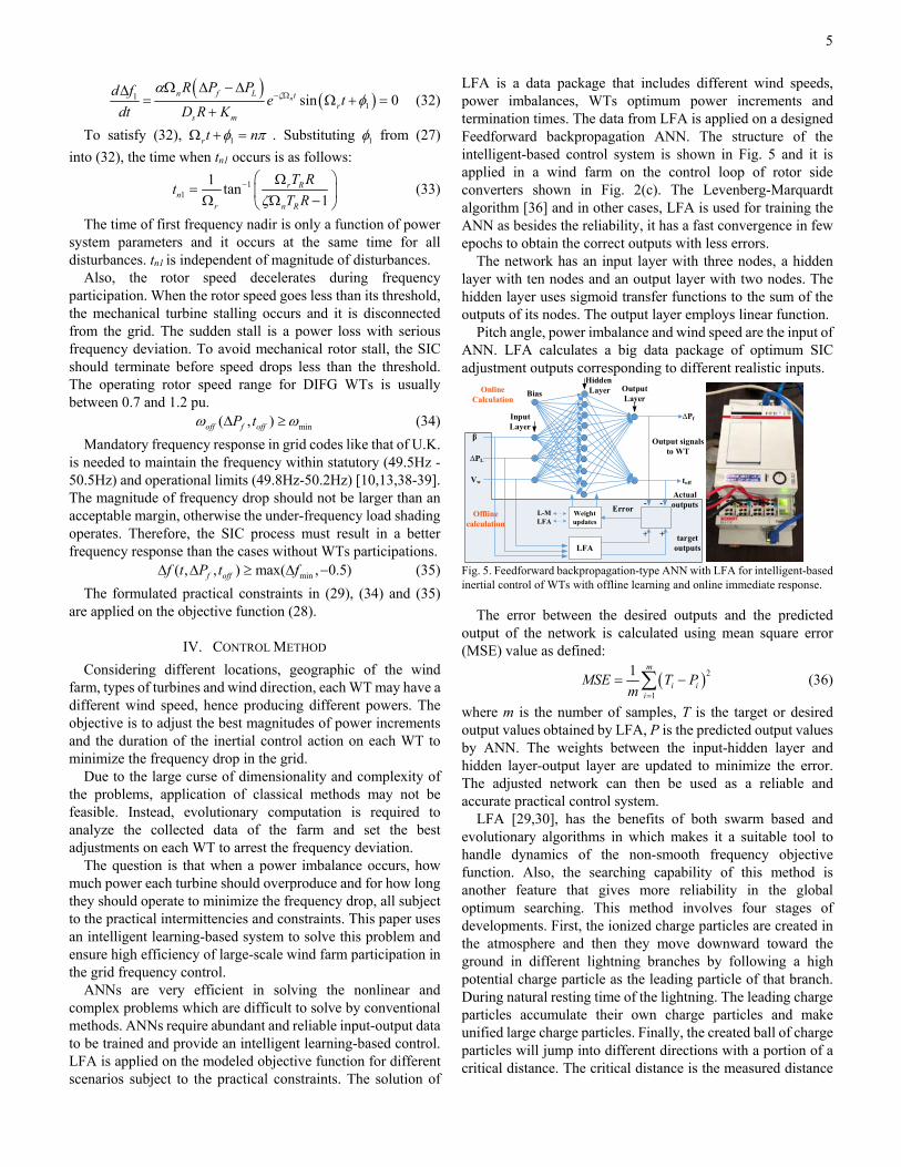
LFA is a data package that includes different wind speeds, power imbalances, WTs optimum power increments and termination times. The data from LFA is applied on a designed Feedforward backpropagation ANN. The structure of the intelligent-based control system is shown in Fig. 5 and it is applied in a wind farm on the control loop of rotor side converters shown in Fig. 2(c). The Levenberg-Marquardt algorithm [36] and in other cases, LFA is used for training the ANN as besides the reliability, it has a fast convergence in few epochs to obtain the correct outputs with less errors.

The network has an input layer with three nodes, a hidden layer with ten nodes and an output layer with two nodes. The hidden layer uses sigmoid transfer functions to the sum of the outputs of its nodes. The output layer employs linear function.

Pitch angle, power imbalance and wind speed are the input of ANN. LFA calculates a big data package of optimum SIC adjustment outputs corresponding to different realistic inputs.

Weight updates

LFA

Error

∆PL

Vw toff

β

Bias

Input Layer

Hidden Layer Output

Layer

Actual outputs

target outputs

Output signals to WT

∆Pf

--

++

L-MLFA

Offline calculation

Online Calculation

Fig. 5. Feedforward backpropagation-type ANN with LFA for intelligent-based inertial control of WTs with offline learning and online immediate response.

The error between the desired outputs and the predicted output of the network is calculated using mean square error (MSE) value as defined:

2

1

1 m

i ii

MSE T Pm

(36)

where m is the number of samples, T is the target or desired output values obtained by LFA, P is the predicted output values by ANN. The weights between the input-hidden layer and hidden layer-output layer are updated to minimize the error. The adjusted network can then be used as a reliable and accurate practical control system.

LFA [29,30], has the benefits of both swarm based and evolutionary algorithms in which makes it a suitable tool to handle dynamics of the non-smooth frequency objective function. Also, the searching capability of this method is another feature that gives more reliability in the global optimum searching. This method involves four stages of developments. First, the ionized charge particles are created in the atmosphere and then they move downward toward the ground in different lightning branches by following a high potential charge particle as the leading particle of that branch. During natural resting time of the lightning. The leading charge particles accumulate their own charge particles and make unified large charge particles. Finally, the created ball of charge particles will jump into different directions with a portion of a critical distance. The critical distance is the measured distance

6

between the leading charge particle and the worst charge particle of a branch. These steps are formulated in (37)-(42).

min max minX X u X X (37)

11 1 1ij ij i ijJ t w J t C u X t X t (38)

1ij ij ijX t J t X t (39)

1 1i i iwD X t X t (40)

i ijX t X t (41)

1ij ij i iX t X t u D (42)

where Xmin and Xmax are the minimum and maximum limits on the objective variables, i.e., toff and ΔPf ; u is the random creation of the agents of the LFA. ijJ refers to the jumping

value of j-th charge particle of the i-th leader; w shows the inertia of the charge particles flowing in the atmosphere; C1 shows that all the charges of a lightning branch can follow the stepped leader of that branch. ijX and iX are the variable of

charge j of leader i, and the stepped leader of the branch i, respectively. The critical distance Di is the measured distance between the worst charge and the stepped leader in the lightning branch i where iwX refers to worst charge in that

channel; αi is the speed of the lightning branch. The algorithm collects the data in the control room and sends

the output signals to the corresponding WTs in the farm. The data analyses and control commands of the wind farm under supervision of LFA can either operate in centralized or the decentralized control systems. Pseudo-code of LFA for SIC of the wind farm is shown in Algorithm 1. Two important parameters of SIC are ΔPf and toff. Obtaining these two parameters lead to inertial control of WTs.

Therefore, the output layer of a neural network can include two neurons. The amount of hidden layer may depend on the dimension of a problem, amount of data, required accuracy, etc. To make a reliable yet simple approximation, seven to ten neurons are considered in this paper.

Algorithm 1 Frequency participation of wind farm using LFA Input: WT, system and LFA parameters Output: [toff ∆Pf] begin For n=1:N % number of WTs in the farm set initial toff,n and ∆Pf,n=0

1. initialize the population at K=0 while ωoff(toff,n, ∆Pf,n) < ωmin or toff,n < tn1

for i=1:Nbranch

toff,n[0]~u(tn1 : toff max,n] ∆Pf,n [0]~u[∆Pf min,n : ∆Pf max,n] X[0]=[toff,n[0] ∆Pf,n [0]]

xp [0]= xp (min F(toff,n[0] ∆Pf,n [0])) & xij,n [0] xi [0] jp[0]=0 end for end while

2. while K≤Kmax a. for i=1:Nbranch & j=1:end b. update Jij[K] , j=1,2,…,end using Eq. (38) c. update position xij,n[K], j=1,2,…,end using Eq. (39) d. while ωoff(toff,n, ∆Pf,n) <ωmin or toff,n<tn1 or |∆f|>0.5

update Xij,n[K] using Eq. (38) and Eq. (39) end while

e. calculate Di using Eq. (40) f. accumulate all charge particles with the branch leader using (41)

Xij,n[K]= Xi,n[K] g. perform jump step using Eq. (42)

h. update the best positions: if F(xij,n[K]) < F(xi,n [K]) xi,n[K+1] ← xij,n[K] else xi,n [K+1] ← xp,n

best[K] end if end for

i. set K=K+1 end while

3. print xi,n[Kmax] end end For Kmax: maximum number of iterations Nbranch: number of lightning branches or lightning leaders F(xij,n[K]): calculated objective function for the n-th WT, i.e., absolute of frequency

drop for value of xij,n[K]=[toff,n[K] ∆Pf,n[K]]. xi,n[K]: the leader of branch i in iteration K for the n-th WT. xi,n[Kmax]: is the best leader with minimum fitness value among the Nbranch leaders in the

last iteration for the n-th WT.

The input layer receives the important dynamic variables, pitch angle β, power imbalance disturbance ΔPL, and the wind speed at the WT vw. By applying the inputs, the weighted sum of the hidden layer is:

(1) (1)(1) (1) (1)1 111 12 13 1

(1) (1)2

(1) (1) (1)(1) (1)71 72 73 37 7

v bw w w x

x W x B

w w w xv b

(43)

where (1)iv is the weighted sum of output node i in the first

layer after the input layer. wij is the weight between the input node j and hidden layer node i. (1)

ib is the bias value of node i of

the hidden layer. The input data of the ANN is presented by x. The output of the nodes at hidden layer is calculated by an

activation function (.) which determines behavior of the

node.

(1 )(1 )11

(1 ) (1 )7 1

vy

y v

(44)

where (1)iy is the output from the corresponding node i of the

hidden layer. In a similar manner the weighted sum of the next layer which is the output layer is calculated:

(1)1(2) (2) (2) (2) (2) (2) (2)(2) (2)

(2) (1) (2)11 12 13 14 15 16 171 1(2) (2) (2) (2) (2) (2) (2)(2) (2)21 22 23 24 25 26 272 2(1)

7

yw w w w w w wv b

W Y Bw w w w w w wv b

y

(45)

(2)(2)11

(2) (2)2 2

vy

y v

(46)

where (2)iv is the weighted sum of output node i in the output

layer. (2)ijw is the weight between the node j of hidden layer and

node i of output layer. (2)ib is the bias value of node i of the

output layer. (2) (2)1 2,y y are the output of the ANN that represent

increment power ΔPf, and the termination time toff. The set of input-output data is applied to the ANN for the

purpose of training and testing. The difference between the actual output data, T and the approximated output of ANN, P (i.e., (2)

iy ) defines an error that can be used as an optimization

function shown in (36). The problem of WT inertial control can be transformed into

the problem of finding the desired set of ANN weight parameters (1) (2),W W and bias values (1) (2),B B . The adequate

adjustment of these parameters leads to a proper approximation

7

of SIC. Optimal weight adjustment of the ANN can be achieved using either Levenberg-Marquardt algorithm or LFA method. Both approaches are used and presented in the paper.

V. SIMULATION AND EXPERIMENTAL VALIDATIONS

A large-scale 100 MW wind farm is integrated into the IEEE 9-bus test system. This test system is particularly suitable for testing novel concepts of power system monitoring, protection and control and has been used since it has been firstly published in [48], Chapter 2.10. Parameters of this test system are today online available, for example using the link [49].

Detailed models of synchronous generators can be also found in [48], Chapters 4 (full-scale detailed model) and 6 (linearized model). Models of the excitation system and governor control are given in Chapters 7 and 10, respectively. Models of synchronous generators can be also found in [50].

As shown in Fig. 6, the wind farm considered in our paper has 20 units of 5 MW DFIG WTs. It was connected to the grid at the bus in which Load 2 (L2) is connected. In the Appendix, some parameters and information about the state of the generators and DFIG are given. A more comprehensive information about the system parameters can be found in [49]. DFIGs were modelled using their full and detailed models [51]. The entire dynamic simulation of the IEEE 9-bus test system was undertaken using DIgSILENT PowerFactory software package [52].

To draw a realistic analysis, the wind farm is operating below rated power while different scenarios are investigated. Different stochastic wind speeds and severe power disturbances are applied to the system to evaluate the performance of the wind farm under the learning-based LFA supervision and ANN prediction. The wind farm is connected to the grid as P-V node to control the active power and voltage at the connection node.

G1 G2

G3

wind farm

L3L1 L2

Fig. 6. Large-scale grid connected wind farm in IEEE 9-bus system.

A. Case one

In this case, the wind farm is considered as an aggregated model with one equivalent WT. The average wind speed value is 10m/s and L3 increases by 35% (35MW) at t0=0s. SIC is

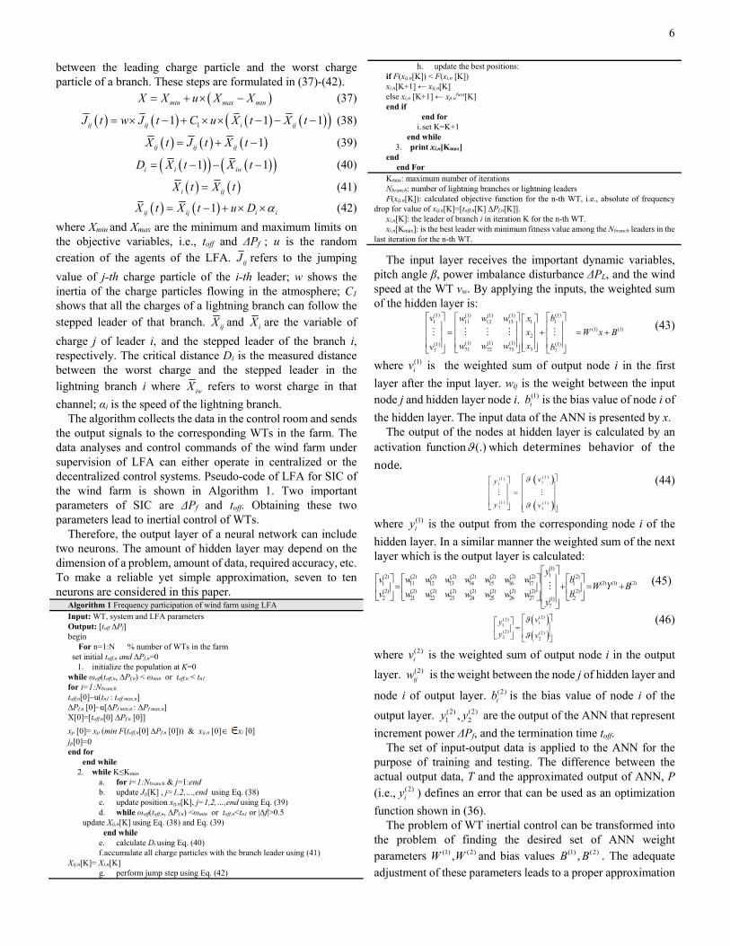
triggered at the same time. Fig. 7 shows the successful frequency control with the provided solutions using LFA in 100 trails. The results of proposed method are compared with the existing SIC scheme explained in literature [40], [41], the modified SIC [42] and SIC temporary over-production (TOP) method [43] shown in Fig. 8. The grid frequency using the proposed control method is better and safer than other quoted methods in literature. Adequate value of ∆Pf has boosted the system’s critical frequency nadir to an optimum and much safer operational value as shown in Fig. 8 (a). Finding the best value of power increment ∆Pf alone is not enough to operate the frequency control of a wind turbine. With the obtained value of power increment, different termination times would result in different frequency excursions in which some may lead to system failure. The best termination time has been obtained as the final frequency control is optimum, shown in Fig. 8 (b).

Fig. 7. Successful frequency response in 100 different trials using LFA.

(a) Grid frequency response using proposed control method.

syst

em f

requ

ency

dro

p (H

z)

(b) Effect of different toff and fixed ∆Pf and the successful performance of LFA with optimum frequency response. Fig. 8. Accurate performance of LFA with optimum frequency response in the power grid; vw=10m/s, ∆PL=0.35 pu

It can be seen that the inertial control power increment and the termination time must be obtained simultaneously to ensure a safe, feasible and optimum power system frequency control using wind power, otherwise, the system without inertial

TABLE I. OPTIMUM TERMINATION TIME AND POWER INCREMENT OF SIC IN DIFFERENT SCENARIOS USING LFA AS SUPERVISED DATA ΔPL(pu)

vw(m/s) 0.1 pu 0.35 pu 0.65 pu 1 pu LFA PSO ICA LFA PSO ICA LFA PSO ICA LFA PSO ICA

8 m/s toff 6.6515 6.8192 6.6511 6.6566 6.658 6.6546 6.6126 4.9197 6.6223 6.559 4.2827 6.5914 ΔPf 0.037543 0.037226 0.037545 0.1315 0.11282 0.13152 0.24221 0.20754 0.24236 0.367 0.23841 0.29978 Δfmax 0.27607 0.2775 0.27607 0.27594 0.2364 0.27591 0.2773 0.3009 0.2772 0.27979 0.3366 0.3095

9 m/s toff 6.6906 6.7126 6.6751 6.6921 6.7027 6.6951 6.673 6.6717 6.6731 6.6044 5.6046 6.6311 ΔPf 0.03659 0.036446 0.036624 0.12883 0.12869 0.12886 0.23799 0.23794 0.23797 0.36172 0.34545 0.36209 Δfmax 0.28028 0.2809 0.28012 0.27931 0.2795 0.27928 0.2802 0.2802 0.28018 0.28212 0.2893 0.28196

10 m/s

toff 6.6931 6.4269 6.6929 6.7334 6.0924 6.7349 6.719 6.7188 6.7201 6.6895 6.6889 6.6886 ΔPf 0.03572 0.03535 0.035718 0.12635 0.12471 0.12637 0.23376 0.23378 0.23379 0.35677 0.35678 0.35679 Δfmax 0.28413 0.2867 0.28413 0.2824 0.28449 0.28242 0.2830 0.2830 0.28303 0.2843 0.2843 0.2843

11 m/s

toff 6.7044 6.6313 6.7025 6.7728 6.7554 6.773 6.767 6.7206 6.7651 6.7425 6.741 6.741 ΔPf 0.034781 0.0348 0.034785 0.12402 0.12342 0.12399 0.2298 0.22883 0.22982 0.35135 0.35138 0.35136 Δfmax 0.2882 0.2901 0.2882 0.28546 0.2861 0.28541 0.28574 0.2864 0.28572 0.2867 0.2867 0.2867

8

control or with improper control adjustments may lead to undesired transients.

Fig. 9. Rotor speed during grid frequency control.

Fig. 10. Stable voltage profile of the system.

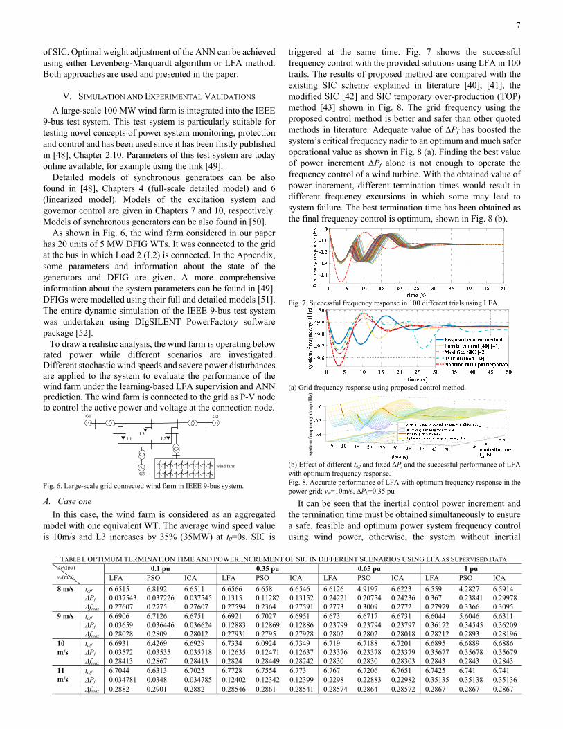
The results of LFA are also compared with finely tuned PSO and ICA as shown in Table I. The parameter settings of these methods can be found in the Appendix. Also, the maximum available power tracking is sufficient to suppress the resonance in a two-mass WT [47]. Once the machine operates in transient grid frequency control, it recovers back to its nominal MPPT mode, faster than other methods that indicates having less stress duration on WT. The mechanical rotor speed recovery is shown in Fig. 9. Besides stable grid frequency, the voltage of the entire system also remains stable as depicted in Fig. 10.

B. Case two

In this case, it is assumed that the wind field in front of the aggregated WT is turbulent and the wind speed could be different after several seconds during SIC process. The wind could be either constant, increasing or decreasing during inertial control. Fixed wind speed was studied in case study A.

Wind speed increases: WT is working at 10m/s where a large disturbance of 0.35 p.u. occurs at t=100s. The SIC is triggered. However, during inertial control process, the wind speed suddenly changes from 10 to 11m/s at t=103s. The performance of SIC scheme and effect of the wind increase is shown in Fig. 11. Generally, wind speed increase during SIC inherently boosts the second frequency nadir because larger wind speed means boosted mechanical power and MPPT curve toward more available kinetic energy. This effect is shown in green color in the figure. Hence, wind speed increase during SIC is beneficial to the process. An intelligent-based controller such as what has been discussed in this paper, can utilize this phenomenon and readjust the WT with the change. Readjustment occurs by adjusting new power increment and/or termination time against the change. This action has been presented by solid blue line.

100 110 120 130 140 150Time (sec.)

49.6

49.8

50

SIC with wind speed=10m/sSIC with wind speed from 10 to 11m/sUpdated SIC with wind speed from 10 to 11m/sNo SIC participation

Fig. 11. Effect of sudden change in wind speed during inertial control.

Fig. 12. Effect of sudden decrease in wind speed during inertial control.

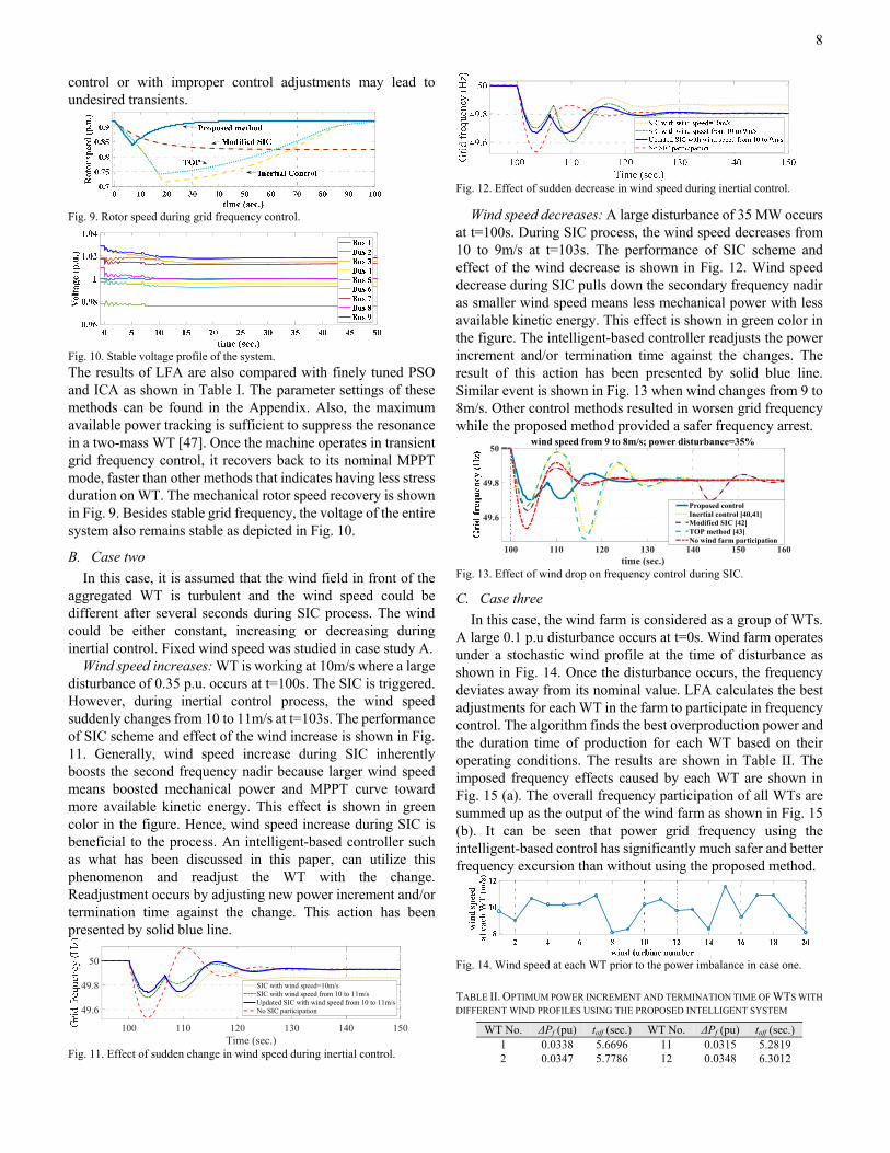
Wind speed decreases: A large disturbance of 35 MW occurs at t=100s. During SIC process, the wind speed decreases from 10 to 9m/s at t=103s. The performance of SIC scheme and effect of the wind decrease is shown in Fig. 12. Wind speed decrease during SIC pulls down the secondary frequency nadir as smaller wind speed means less mechanical power with less available kinetic energy. This effect is shown in green color in the figure. The intelligent-based controller readjusts the power increment and/or termination time against the changes. The result of this action has been presented by solid blue line. Similar event is shown in Fig. 13 when wind changes from 9 to 8m/s. Other control methods resulted in worsen grid frequency while the proposed method provided a safer frequency arrest.

100 110 120 130 140 150 160time (sec.)

49.6

49.8

50wind speed from 9 to 8m/s; power disturbance=35%

Proposed controlInertial control [40,41]Modified SIC [42]TOP method [43]No wind farm participation

Fig. 13. Effect of wind drop on frequency control during SIC.

C. Case three

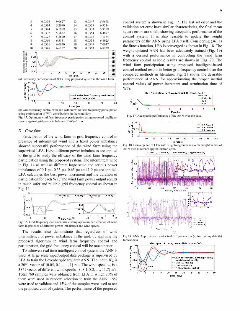
In this case, the wind farm is considered as a group of WTs. A large 0.1 p.u disturbance occurs at t=0s. Wind farm operates under a stochastic wind profile at the time of disturbance as shown in Fig. 14. Once the disturbance occurs, the frequency deviates away from its nominal value. LFA calculates the best adjustments for each WT in the farm to participate in frequency control. The algorithm finds the best overproduction power and the duration time of production for each WT based on their operating conditions. The results are shown in Table II. The imposed frequency effects caused by each WT are shown in Fig. 15 (a). The overall frequency participation of all WTs are summed up as the output of the wind farm as shown in Fig. 15 (b). It can be seen that power grid frequency using the intelligent-based control has significantly much safer and better frequency excursion than without using the proposed method.

Fig. 14. Wind speed at each WT prior to the power imbalance in case one.

TABLE II. OPTIMUM POWER INCREMENT AND TERMINATION TIME OF WTS WITH

DIFFERENT WIND PROFILES USING THE PROPOSED INTELLIGENT SYSTEM

WT No. ΔPf (pu) toff (sec.) WT No. ΔPf (pu) toff (sec.) 1 0.0338 5.6696 11 0.0315 5.2819 2 0.0347 5.7786 12 0.0348 6.3012

9

3 0.0308 9.0627 13 0.0347 5.9698 4 0.0314 5.2090 14 0.0359 6.9214 5 0.0344 6.1959 15 0.0333 5.9709 6 0.0332 5.5652 16 0.0354 6.4877 7 0.0327 5.5670 17 0.0336 7.1184 8 0.0366 6.5131 18 0.0338 6.8925 9 0.0361 6.0870 19 0.0349 7.0037 10 0.0348 6.6157 20 0.0363 6.8229

Fre

qu

ency

dev

iati

on o

f W

Ts

du

rin

g S

IC (

Hz)

(a) Frequency participation of WTs using proposed system in the wind farm

(b) Grid frequency control with and without wind farm frequency participation using optimization of WTs contributions in the wind farm Fig. 15. Optimum wind farm frequency participation using proposed intelligent system against grid power imbalance of ∆PL=0.1pu.

D. Case four

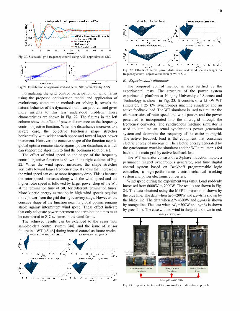
Participation of the wind farm in grid frequency control in presence of intermittent wind and a fixed power imbalance showed successful performance of the wind farm using the supervised LFA. Here, different power imbalances are applied to the grid to study the efficacy of the wind farm frequency participation using the proposed system. The intermittent wind in Fig. 14 as well as different large scale and serious power imbalances of 0.1 pu, 0.35 pu, 0.65 pu and 1.0 pu are applied. LFA calculates the best power increment and the duration of participation for each WT. The wind farm power output results in much safer and reliable grid frequency control as shown in Fig. 16.

Gri

d f

req

uen

cy (

Hz)

Fig. 16. Grid frequency excursion arrest using optimum participation of wind farm in presence of different power imbalances and wind speeds.

The results also demonstrate that regardless of wind intermittency or power imbalance in the grid, by applying the proposed algorithm in wind farm frequency control and participation, the grid frequency control will be much better.

To achieve a real time intelligent control system, the ANN is used. A large scale input/output data package is supervised by LFA to train the Levenberg-Marquardt ANN. The input ΔPL is a 20*1 vector of 0.05, 0.1, … , 1 p.u. The wind speed vw is a 38*1 vector of different wind speeds 8, 8.1, 8.2, …, 11.7m/s. Total 760 samples were obtained from LFA in which 70% of them were used in random selection to train the ANN, 15% were used to validate and 15% of the samples were used to test the proposed control system. The performance of the proposed

control system is shown in Fig. 17. The test set error and the validation set error have similar characteristics, the final mean square errors are small, showing acceptable performance of the control system. It is also feasible to update the weight parameters of the ANN using LFA itself. Considering (36) as the fitness function, LFA is converged as shown in Fig. 18. The weight updated ANN has been adequately trained (Fig. 19) with a desired performance in controlling the wind farm frequency control as some results are shown in Figs. 20. The wind farm participation using proposed intelligent-based control method results in better grid frequency control than the compared methods in literature. Fig. 21 shows the desirable performance of ANN for approximating the proper inertial control values of power increment and termination time of WTs.

Fig. 17. Acceptable performance of the ANN over the data.

Fig. 18. Convergence of LFA with 3 lightning branches to the weight values of ANN with minimum approximation error.

(b)

Fig 19. ANN Approximated and actual SIC parameters (a) for training data (b) for test data

10

Fig. 20. Successful grid frequency control using ANN approximated SIC.

Fig 21. Distribution of approximated and actual SIC parameters by ANN.

Formulating the grid control participation of wind farms using the proposed optimization model and application of evolutionary computation methods on solving it, reveals the natural behavior of the dynamical nonlinear problem and gives more insights to this less understood problem. These characteristics are shown in Fig. 22. The figures in the left column show the effect of power disturbance on the frequency control objective function. When the disturbance increases to a severe case, the objective function’s shape stretches horizontally with wider search space and toward larger power increment. However, the concave shape of the function near its global optima remains stable against power disturbances which can support the algorithm to find the optimum solution set.

The effect of wind speed on the shape of the frequency control objective function is shown in the right column of Fig. 22. When the wind speed increases, the shape stretches vertically toward larger frequency dip. It shows that increase in the wind speed can cause more frequency drop. This is because the rotor speed increases along with the wind speed and the higher rotor speed is followed by larger power drop of the WT at the termination time of SIC for different termination times. More kinetic energy extraction in high wind speeds requires more power from the grid during recovery stage. However, the concave shape of the function near its global optima remains stable against intermittent wind speed. These effect indicate that only adequate power increment and termination times must be considered in SIC schemes in the wind farms.

The achieved results can be extended to the cases with sampled-data control system [44], and the issue of sensor failure in a WT [45,46] during inertial control as future works.

Fig. 22. Effects of active power disturbance and wind speed changes on frequency control objective function of WT’s SIC.

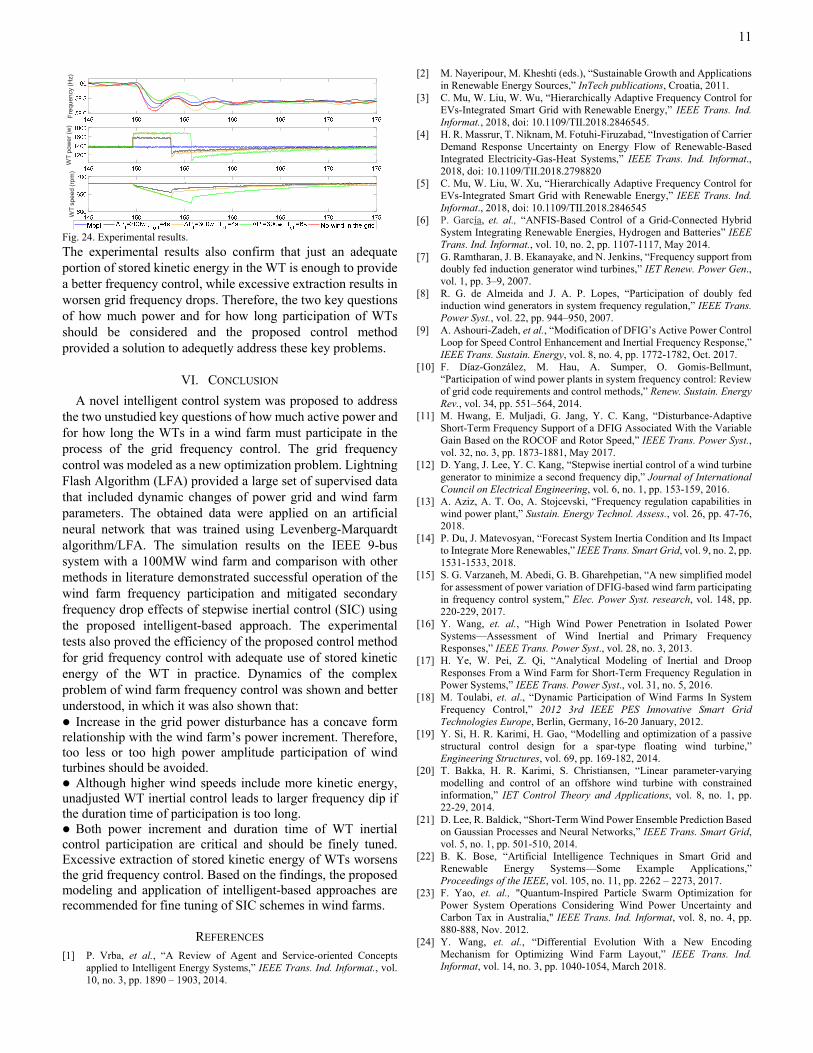
E. Experimental validations

The proposed control method is also verified by the experimental tests. The structure of the power system experimental platform at Nanjing University of Science and Technology is shown in Fig. 23. It consists of a 15 kW WT simulator, a 25 kW synchronous machine simulator and an active feedback load. The WT simulator is used to simulate the characteristics of rotor speed and wind power, and the power generated is incorporated into the microgrid through the frequency converter. The synchronous machine simulator is used to simulate an actual synchronous power generation system and determine the frequency of the entire microgrid. The active feedback load is the equipment that consumes electric energy of microgrid. The electric energy generated by the synchronous machine simulator and the WT simulator is fed back to the main grid by active feedback load.

The WT simulator consists of a 3-phase induction motor, a permanent magnet synchronous generator, real time digital control system based on Beckhoff programmable logic controller, a high-performance electromechanical tracking system and power electronic converters.

Wind speed during the experiment was 6m/s. Load suddenly increased from 6000W to 7000W. The results are shown in Fig. 24. The data obtained using the MPPT operation is shown by the blue line. The data when ∆Pf =200W and toff=4s is shown by the black line. The data when ∆Pf =300W and toff=4s is shown by orange line. The data when ∆Pf =300W and toff=6s is shown by green line. The case with no wind in the grid is shown in red.

Main grid: 400V, 50Hz

Microgrid: 400V, 60Hz

Active Feedback Load

Wind Turbine Simulator

Inverter

Rectifier

Motor Drive

Rectifier

Inverter

ACMotor

PMSG

Synchronous Machine Simulator

ACMotor

SynchronousGenerator

Fig. 23. Experimental tests of the proposed inertial control approach

11

Fre

que

ncy

(H

z)W

T p

ow

er

(w)

WT

sp

ee

d (

rpm

)

Fig. 24. Experimental results.

The experimental results also confirm that just an adequate portion of stored kinetic energy in the WT is enough to provide a better frequency control, while excessive extraction results in worsen grid frequency drops. Therefore, the two key questions of how much power and for how long participation of WTs should be considered and the proposed control method provided a solution to adequetly address these key problems.

VI. CONCLUSION

A novel intelligent control system was proposed to address the two unstudied key questions of how much active power and for how long the WTs in a wind farm must participate in the process of the grid frequency control. The grid frequency control was modeled as a new optimization problem. Lightning Flash Algorithm (LFA) provided a large set of supervised data that included dynamic changes of power grid and wind farm parameters. The obtained data were applied on an artificial neural network that was trained using Levenberg-Marquardt algorithm/LFA. The simulation results on the IEEE 9-bus system with a 100MW wind farm and comparison with other methods in literature demonstrated successful operation of the wind farm frequency participation and mitigated secondary frequency drop effects of stepwise inertial control (SIC) using the proposed intelligent-based approach. The experimental tests also proved the efficiency of the proposed control method for grid frequency control with adequate use of stored kinetic energy of the WT in practice. Dynamics of the complex problem of wind farm frequency control was shown and better understood, in which it was also shown that: Increase in the grid power disturbance has a concave form relationship with the wind farm’s power increment. Therefore, too less or too high power amplitude participation of wind turbines should be avoided. Although higher wind speeds include more kinetic energy, unadjusted WT inertial control leads to larger frequency dip if the duration time of participation is too long. Both power increment and duration time of WT inertial control participation are critical and should be finely tuned. Excessive extraction of stored kinetic energy of WTs worsens the grid frequency control. Based on the findings, the proposed modeling and application of intelligent-based approaches are recommended for fine tuning of SIC schemes in wind farms.

REFERENCES [1] P. Vrba, et al., “A Review of Agent and Service-oriented Concepts

applied to Intelligent Energy Systems,” IEEE Trans. Ind. Informat., vol. 10, no. 3, pp. 1890 – 1903, 2014.

[2] M. Nayeripour, M. Kheshti (eds.), “Sustainable Growth and Applications in Renewable Energy Sources,” InTech publications, Croatia, 2011.

[3] C. Mu, W. Liu, W. Wu, “Hierarchically Adaptive Frequency Control for EVs-Integrated Smart Grid with Renewable Energy,” IEEE Trans. Ind. Informat., 2018, doi: 10.1109/TII.2018.2846545.

[4] H. R. Massrur, T. Niknam, M. Fotuhi-Firuzabad, “Investigation of Carrier Demand Response Uncertainty on Energy Flow of Renewable-Based Integrated Electricity-Gas-Heat Systems,” IEEE Trans. Ind. Informat., 2018, doi: 10.1109/TII.2018.2798820

[5] C. Mu, W. Liu, W. Xu, “Hierarchically Adaptive Frequency Control for EVs-Integrated Smart Grid with Renewable Energy,” IEEE Trans. Ind. Informat., 2018, doi: 10.1109/TII.2018.2846545

[6] P. García, et. al., “ANFIS-Based Control of a Grid-Connected Hybrid System Integrating Renewable Energies, Hydrogen and Batteries” IEEE Trans. Ind. Informat., vol. 10, no. 2, pp. 1107-1117, May 2014.

[7] G. Ramtharan, J. B. Ekanayake, and N. Jenkins, “Frequency support from doubly fed induction generator wind turbines,” IET Renew. Power Gen., vol. 1, pp. 3–9, 2007.

[8] R. G. de Almeida and J. A. P. Lopes, “Participation of doubly fed induction wind generators in system frequency regulation,” IEEE Trans. Power Syst., vol. 22, pp. 944–950, 2007.

[9] A. Ashouri-Zadeh, et al., “Modification of DFIG’s Active Power Control Loop for Speed Control Enhancement and Inertial Frequency Response,” IEEE Trans. Sustain. Energy, vol. 8, no. 4, pp. 1772-1782, Oct. 2017.

[10] F. Díaz-González, M. Hau, A. Sumper, O. Gomis-Bellmunt, “Participation of wind power plants in system frequency control: Review of grid code requirements and control methods,” Renew. Sustain. Energy Rev., vol. 34, pp. 551–564, 2014.

[11] M. Hwang, E. Muljadi, G. Jang, Y. C. Kang, “Disturbance-Adaptive Short-Term Frequency Support of a DFIG Associated With the Variable Gain Based on the ROCOF and Rotor Speed,” IEEE Trans. Power Syst., vol. 32, no. 3, pp. 1873-1881, May 2017.

[12] D. Yang, J. Lee, Y. C. Kang, “Stepwise inertial control of a wind turbine generator to minimize a second frequency dip,” Journal of International Council on Electrical Engineering, vol. 6, no. 1, pp. 153-159, 2016.

[13] A. Aziz, A. T. Oo, A. Stojcevski, “Frequency regulation capabilities in wind power plant,” Sustain. Energy Technol. Assess., vol. 26, pp. 47-76, 2018.

[14] P. Du, J. Matevosyan, “Forecast System Inertia Condition and Its Impact to Integrate More Renewables,” IEEE Trans. Smart Grid, vol. 9, no. 2, pp. 1531-1533, 2018.

[15] S. G. Varzaneh, M. Abedi, G. B. Gharehpetian, “A new simplified model for assessment of power variation of DFIG-based wind farm participating in frequency control system,” Elec. Power Syst. research, vol. 148, pp. 220-229, 2017.

[16] Y. Wang, et. al., “High Wind Power Penetration in Isolated Power Systems—Assessment of Wind Inertial and Primary Frequency Responses,” IEEE Trans. Power Syst., vol. 28, no. 3, 2013.

[17] H. Ye, W. Pei, Z. Qi, “Analytical Modeling of Inertial and Droop Responses From a Wind Farm for Short-Term Frequency Regulation in Power Systems,” IEEE Trans. Power Syst., vol. 31, no. 5, 2016.

[18] M. Toulabi, et. al., “Dynamic Participation of Wind Farms In System Frequency Control,” 2012 3rd IEEE PES Innovative Smart Grid Technologies Europe, Berlin, Germany, 16-20 January, 2012.

[19] Y. Si, H. R. Karimi, H. Gao, “Modelling and optimization of a passive structural control design for a spar-type floating wind turbine,” Engineering Structures, vol. 69, pp. 169-182, 2014.

[20] T. Bakka, H. R. Karimi, S. Christiansen, “Linear parameter-varying modelling and control of an offshore wind turbine with constrained information,” IET Control Theory and Applications, vol. 8, no. 1, pp. 22-29, 2014.

[21] D. Lee, R. Baldick, “Short-Term Wind Power Ensemble Prediction Based on Gaussian Processes and Neural Networks,” IEEE Trans. Smart Grid, vol. 5, no. 1, pp. 501-510, 2014.

[22] B. K. Bose, “Artificial Intelligence Techniques in Smart Grid and Renewable Energy Systems—Some Example Applications,” Proceedings of the IEEE, vol. 105, no. 11, pp. 2262 – 2273, 2017.

[23] F. Yao, et. al., "Quantum-Inspired Particle Swarm Optimization for Power System Operations Considering Wind Power Uncertainty and Carbon Tax in Australia," IEEE Trans. Ind. Informat, vol. 8, no. 4, pp. 880-888, Nov. 2012.

[24] Y. Wang, et. al., “Differential Evolution With a New Encoding Mechanism for Optimizing Wind Farm Layout,” IEEE Trans. Ind. Informat, vol. 14, no. 3, pp. 1040-1054, March 2018.

12

[25] L. Wang, "Wind Turbine Gearbox Failure Identification With Deep Neural Networks," IEEE Trans. Ind. Informat, vol. 13, no. 3, pp. 1360-1368, June 2017.

[26] E. Alizadeh, N. Meskin, K. Khorasani, “A Dendritic Cell Immune System Inspired Scheme for Sensor Fault Detection and Isolation of Wind Turbines,” IEEE Trans. Ind. Informat, vol. 14, no. 2, pp. 545-555, 2018.

[27] B. Yang, R. Liu, X. Chen, “Fault Diagnosis for a Wind Turbine Generator Bearing via Sparse Representation and Shift-Invariant K-SVD” IEEE Trans. Ind. Informat., vol. 13, no. 3, pp. 1321-1331, 2017.

[28] R. Wang, et. al,, “A Graph Theory Based Energy Routing Algorithm in Energy Local Area Network,” IEEE Trans. Ind. Informat., vol. 13, no. 6, pp. 3275-3285, Dec. 2017.

[29] M. Kheshti, et al., “An effective Lightning Flash Algorithm solution to large scale non-convex economic dispatch with valve-point and multiple fuel options on generation units,” Energy, vol. 129, pp. 1-15, 2017.

[30] M. Kheshti, et al., “Lightning Flash Algorithm for Solving Nonconvex Combined Emission Economic Dispatch with Generator Constraints,” IET Gener. Transm. Distrib., vol. 12, no. 1, pp. 104-116, 2018

[31] J. Kennedy, R. C. Eberhart, “particle swarm optimization,” in: 4th IEEE International Conference on Neural Networks (ICNN), Perth, Australia, 27 November-01 December 1995, pp. 1942-1948.

[32] E. Atashpaz-Gargari, C. Lucas, “Imperialist competitive algorithm: an algorithm for optimization inspired by imperialistic competition,” In: IEEE congress on evolutionary computation, Singapore, 2007, pp. 4661-4667.

[33] P. M. Anderson, M. Mirheydar, “A Low-Order System Frequency Response Model,” IEEE Trans. Power Syst., vol. 5, pp. 720–729, 1990.

[34] K. Ogata, “Modern Control Engineering” 4th ed., Prentice-Hall, 2002, USA.

[35] J. L. Schiff, “The Laplace Transform: Theory and Applications,” 1st ed., Springer, 1999, USA.

[36] D. W. Marquardt. “An algorithm for least-squares estimation of nonlinear parameters,” J. Soc. Indust. Appl. Math., 11(2):431-441, 1963.

[37] A. De Paola, D. Angeli, G. Strbac, “Scheduling of Wind Farms for Optimal Frequency Response and Energy Recovery,” IEEE Trans. Control Syst., vol. 24, no. 5, pp. 1764-1778, 2016.

[38] National Grid. Mandatory Frequency Response | National Grid; 2016. [online] Available at: http://www.nationalgrid.com.

[39] National Grid. Guidance notes-Power park module; 2012. Available at: www.nationalgrid.com/uk.

[40] N. R. Ullah, T. Thiringer, D. Karlsson, “Temporary Primary Frequency Control Support by Variable Speed Wind Turbines—Potential and Applications” IEEE Trans. Power Syst., vol. 23, no. 2, pp. 601-612, 2008.

[41] M. Kang, E. Muljadi, K. Hur, Y. C. Kang, “Stable Adaptive Inertial Control of a Doubly-Fed Induction Generator,” IEEE Trans. Smart Grid, vol. 7, no. 6, pp. 2971-2979, November 2016.

[42] M. Kang, J. Lee, Y. C. Kang, “Modified stepwise inertial control using the mechanical input and electrical output curves of a doubly fed induction generator,” 9th International Conference on Power Electronics-ECCE Asia, June 1-5, 2015, Seoul, Korea.

[43] G. C. Tarnowski, P. C. Kjær, P. Sørensen, J. Østergaard, “Variable Speed Wind Turbines Capability for Temporary Over- Production”, 2009 IEEE Power & Energy Society General Meeting, 2 Oct. 2009, Calgary, Canada.

[44] J. Cheng, J. H. Park, H. R. Karimi, H. Shen, “A Flexible Terminal Approach to Sampled-Data Exponentially Synchronization of Markovian Neural Networks With Time-Varying Delayed Signals,” IEEE Trans. Cybern., vol. 48, no. 8, pp. 2232-2244, August 2018.

[45] S. K. Kommuri, M. Defoort, H. R. Karimi, K. C. Veluvolu, “A Robust Observer-Based Sensor Fault-Tolerant Control for PMSM in Electric Vehicles” IEEE Trans. Ind. Electron.,vol.63, no.12, pp. 7671-7681, 2016.

[46] Y. Li, H. R. Karimi, Q. Zhang, D. Zhao, Y. Li, “Fault Detection for Linear Discrete Time-Varying Systems Subject to Random Sensor Delay: A Riccati Equation Approach,” IEEE Trans. Circuits Syst. I, Reg. Papers, vol. 65, no. 5, pp. 1707-1716, May 2018.

[47] M.F.M. Arani, Y. A. R. I. Mohamed, “Analysis and Mitigation of Undesirable Impacts of Implementing Frequency Support Controllers in Wind Power Generation” IEEE Trans. Energy Convers., vol. 31, no. 1, pp. 174-186, 2016.

[48] P. M. Anderson, A. A. Fouad, “Power System Control and Stability” 2nd ed., IEEE Press, 2003, USA.

[49] “Dynamic IEEE test system” [Online]. Available: http://www.kios.ucy.ac.cy/testsystems/

[50] P. Kundur, “Power System Stability and Control” McGraw-Hill, New York, 1994.

[51] D. Xu, F. Blaabjerg, W. Chen, N. Zhu, “Advanced Control of Doubly Fed Induction Generator for Wind Power Systems” Wiley-IEEE Press, 2018.

[52] Digsilent PowerFactory 15.1, DIgSILENT GmbH, 2015.

APPENDIX TABLE A.1. PARAMETERS OF THE DFIG

Parameters Units Value Rated Apparent Power kVA 5556 Rated Mechanical Power kW 4869.553 Number of Pole Pairs - 2 Rated Voltage kV 0.69 Nominal Speed rpm 1485.153 Stator Resistance p.u. 0.01 Stator Reactance p.u. 0.1 Magnetizing Reactance p.u. 3.5 Rotor Resistance p.u. 0.056 Rotor Reactance p.u. 0.031 Coefficient of MPPT control (Kopt) - 0.4993

TABLE A.2. TERMINAL CONDITIONS OF IEEE 9-BUS SYSTEM

Bus V [kV] nominal power [MW] P [MW] Q [Mvar] 1 16.5 247.5 50 27 2 18.0 212.5 163 10 3 13.8 170 85 0

TABLE A.3. LOAD CHARACTERISTICS OF IEEE 9-BUS SYSTEM

Bus P [MW] Q [Mvar] 5 125 40 6 90 30 8 100 35

TABLE A.4. TRANSMISSION LINE CHARACTERISTICS OF IEEE 9-BUS SYSTEM

Line R [Ω/km] X [Ω/km]

From Bus To Bus 4 5 5.29 44.965 4 6 8.993 48.668 5 7 16.928 85.169 6 9 20.631 89.93 7 8 4.4965 38.088 8 9 6.2951 53.3232

TABLE A.5. SFR PARAMETERS

Hs Ds Km FH TR R

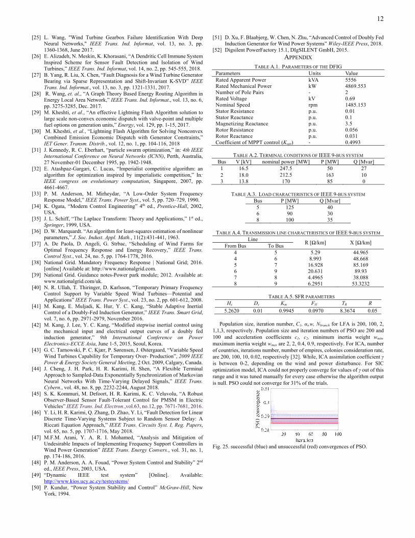
5.2620 0.01 0.9945 0.0970 8.3674 0.05 Population size, iteration number, C1, αi,w, Nbranch for LFA is 200, 100, 2,

1,1,3, respectively. Population size and iteration numbers of PSO are 200 and 100 and acceleration coefficients c1, c2, minimum inertia weight wmin, maximum inertia weight wmax are 2, 2, 0.4, 0.9, respectively. For ICA, number of countries, iterations number, number of empires, colonies consideration rate, are 200, 100, 10, 0.02, respectively [32]. While, ICA assimilation coefficient γ is between 0-2, depending on the wind and power disturbance. For SIC optimization model, ICA could not properly converge for values of γ out of this range and it was tuned manually for every case otherwise the algorithm output is null. PSO could not converge for 31% of the trials.

Fig. 25. successful (blue) and unsuccessful (red) convergences of PSO.