Embed Size (px)
Citation preview
Topics on Modelling and Simulation of Wireless Networking Protocols
A Thesis
Submitted to the Faculty
of
Drexel University
by
Jeffrey W. Wildman II
in partial fulfillment of the
requirements for the degree
of
Master of Science in Electrical and Computer Engineering
April 2009

c© Copyright April 2009Jeffrey W. Wildman II. All Rights Reserved.

Dedications
To my grandmother, Joycelyn S. Wildman

Acknowledgements
Many thanks to:
Dr. Moshe Kam and Dr. Steven Weber, my advisors, for all of their guidance and advice
Dr. Siamak Dastangoo, for the opportunity to learn and work at MIT Lincoln Lab,
Dr. Glenn Carl, for his emulation testbed work and constructive criticism,
past and current labmates at the Data Fusion Lab and ACIN,
my friends for putting up with my frequent aloofness,
my family for the two-day getaways called weekends,
and
Becky, for her patience, love, and support.
i
Table of Contents
List of Figures . . . . . . . . . . . . . . . . . . . . . . . . . . . . . . . . . . . . . . . . . . . . . . . . . . . . . . . . . . . . . . . . . . . . . . . . . . . . . . . . . . . . . . . . . iv
List of Tables . . . . . . . . . . . . . . . . . . . . . . . . . . . . . . . . . . . . . . . . . . . . . . . . . . . . . . . . . . . . . . . . . . . . . . . . . . . . . . . . . . . . . . . . . . vi
List of Acronyms . . . . . . . . . . . . . . . . . . . . . . . . . . . . . . . . . . . . . . . . . . . . . . . . . . . . . . . . . . . . . . . . . . . . . . . . . . . . . . . . . . . . . . vii
Abstract . . . . . . . . . . . . . . . . . . . . . . . . . . . . . . . . . . . . . . . . . . . . . . . . . . . . . . . . . . . . . . . . . . . . . . . . . . . . . . . . . . . . . . . . . . . . . . . . x
1. Introduction . . . . . . . . . . . . . . . . . . . . . . . . . . . . . . . . . . . . . . . . . . . . . . . . . . . . . . . . . . . . . . . . . . . . . . . . . . . . . . . . . . . . . . . . 1
2. RTS-CTS Abstractions . . . . . . . . . . . . . . . . . . . . . . . . . . . . . . . . . . . . . . . . . . . . . . . . . . . . . . . . . . . . . . . . . . . . . . . . . . . . 3
2.1 Introduction. . . . . . . . . . . . . . . . . . . . . . . . . . . . . . . . . . . . . . . . . . . . . . . . . . . . . . . . . . . . . . . . . . . . . . . . . . . . . . . . . . . . . . . 3
2.2 Survey of Literature on Simulation Performance . . . . . . . . . . . . . . . . . . . . . . . . . . . . . . . . . . . . . . . . . . . . . . 4
2.3 Custom-built Simulator Models . . . . . . . . . . . . . . . . . . . . . . . . . . . . . . . . . . . . . . . . . . . . . . . . . . . . . . . . . . . . . . . . . 5
2.3.1 Mobility . . . . . . . . . . . . . . . . . . . . . . . . . . . . . . . . . . . . . . . . . . . . . . . . . . . . . . . . . . . . . . . . . . . . . . . . . . . . . . . . . . . . . . . . . 5
2.3.2 Traffic . . . . . . . . . . . . . . . . . . . . . . . . . . . . . . . . . . . . . . . . . . . . . . . . . . . . . . . . . . . . . . . . . . . . . . . . . . . . . . . . . . . . . . . . . . . 5
2.3.3 Transmission. . . . . . . . . . . . . . . . . . . . . . . . . . . . . . . . . . . . . . . . . . . . . . . . . . . . . . . . . . . . . . . . . . . . . . . . . . . . . . . . . . . . 5
2.4 IEEE 802.11 Model Abstractions . . . . . . . . . . . . . . . . . . . . . . . . . . . . . . . . . . . . . . . . . . . . . . . . . . . . . . . . . . . . . . . 7
2.4.1 Event-Compression Model . . . . . . . . . . . . . . . . . . . . . . . . . . . . . . . . . . . . . . . . . . . . . . . . . . . . . . . . . . . . . . . . . . . . . 7
2.4.2 Neighbor List Model . . . . . . . . . . . . . . . . . . . . . . . . . . . . . . . . . . . . . . . . . . . . . . . . . . . . . . . . . . . . . . . . . . . . . . . . . . . 9
2.4.3 Simplified Neighbor List . . . . . . . . . . . . . . . . . . . . . . . . . . . . . . . . . . . . . . . . . . . . . . . . . . . . . . . . . . . . . . . . . . . . . . . 10
2.5 OPNET Validation Model . . . . . . . . . . . . . . . . . . . . . . . . . . . . . . . . . . . . . . . . . . . . . . . . . . . . . . . . . . . . . . . . . . . . . . . 11
2.6 Simulation Results . . . . . . . . . . . . . . . . . . . . . . . . . . . . . . . . . . . . . . . . . . . . . . . . . . . . . . . . . . . . . . . . . . . . . . . . . . . . . . . 12
2.7 Conclusion . . . . . . . . . . . . . . . . . . . . . . . . . . . . . . . . . . . . . . . . . . . . . . . . . . . . . . . . . . . . . . . . . . . . . . . . . . . . . . . . . . . . . . . . 16
3. IPv6 Address Autoconfiguration . . . . . . . . . . . . . . . . . . . . . . . . . . . . . . . . . . . . . . . . . . . . . . . . . . . . . . . . . . . . . . . . . 18
3.1 Introduction. . . . . . . . . . . . . . . . . . . . . . . . . . . . . . . . . . . . . . . . . . . . . . . . . . . . . . . . . . . . . . . . . . . . . . . . . . . . . . . . . . . . . . . 18
3.2 Autoconfiguration Approaches and Related Work . . . . . . . . . . . . . . . . . . . . . . . . . . . . . . . . . . . . . . . . . . . . . 19
3.2.1 Stateful Autoconfiguration . . . . . . . . . . . . . . . . . . . . . . . . . . . . . . . . . . . . . . . . . . . . . . . . . . . . . . . . . . . . . . . . . . . . 19
3.2.2 Stateless Autoconfiguration . . . . . . . . . . . . . . . . . . . . . . . . . . . . . . . . . . . . . . . . . . . . . . . . . . . . . . . . . . . . . . . . . . . 19
3.2.3 Hybrid Autoconfiguration . . . . . . . . . . . . . . . . . . . . . . . . . . . . . . . . . . . . . . . . . . . . . . . . . . . . . . . . . . . . . . . . . . . . . 20
3.2.4 Duplicate Address Detection . . . . . . . . . . . . . . . . . . . . . . . . . . . . . . . . . . . . . . . . . . . . . . . . . . . . . . . . . . . . . . . . . . 20
3.2.5 MANET Autoconfiguration . . . . . . . . . . . . . . . . . . . . . . . . . . . . . . . . . . . . . . . . . . . . . . . . . . . . . . . . . . . . . . . . . . . 21
3.2.6 Military Networks and Mobility Models. . . . . . . . . . . . . . . . . . . . . . . . . . . . . . . . . . . . . . . . . . . . . . . . . . . . . . 22
3.3 Prefix Continuity . . . . . . . . . . . . . . . . . . . . . . . . . . . . . . . . . . . . . . . . . . . . . . . . . . . . . . . . . . . . . . . . . . . . . . . . . . . . . . . . . 23
3.4 Network Environment . . . . . . . . . . . . . . . . . . . . . . . . . . . . . . . . . . . . . . . . . . . . . . . . . . . . . . . . . . . . . . . . . . . . . . . . . . . . 24
ii
3.5 General Simulation Details . . . . . . . . . . . . . . . . . . . . . . . . . . . . . . . . . . . . . . . . . . . . . . . . . . . . . . . . . . . . . . . . . . . . . . 26
3.5.1 Prefix Continuity Model . . . . . . . . . . . . . . . . . . . . . . . . . . . . . . . . . . . . . . . . . . . . . . . . . . . . . . . . . . . . . . . . . . . . . . . 27
3.5.2 Mobility Models . . . . . . . . . . . . . . . . . . . . . . . . . . . . . . . . . . . . . . . . . . . . . . . . . . . . . . . . . . . . . . . . . . . . . . . . . . . . . . . . 27
3.5.3 Performance Metrics . . . . . . . . . . . . . . . . . . . . . . . . . . . . . . . . . . . . . . . . . . . . . . . . . . . . . . . . . . . . . . . . . . . . . . . . . . . 28
3.6 Simulation Scenarios . . . . . . . . . . . . . . . . . . . . . . . . . . . . . . . . . . . . . . . . . . . . . . . . . . . . . . . . . . . . . . . . . . . . . . . . . . . . . 29
3.6.1 Validation Scenario . . . . . . . . . . . . . . . . . . . . . . . . . . . . . . . . . . . . . . . . . . . . . . . . . . . . . . . . . . . . . . . . . . . . . . . . . . . . 29
3.6.2 Scenario I: Single, Stationary Gateway . . . . . . . . . . . . . . . . . . . . . . . . . . . . . . . . . . . . . . . . . . . . . . . . . . . . . . . 29
3.6.3 Scenario II: Single, Mobile Gateway . . . . . . . . . . . . . . . . . . . . . . . . . . . . . . . . . . . . . . . . . . . . . . . . . . . . . . . . . . 30
3.6.4 Scenario III: Multiple, Mobile Gateways . . . . . . . . . . . . . . . . . . . . . . . . . . . . . . . . . . . . . . . . . . . . . . . . . . . . . 30
3.7 Simulation Results . . . . . . . . . . . . . . . . . . . . . . . . . . . . . . . . . . . . . . . . . . . . . . . . . . . . . . . . . . . . . . . . . . . . . . . . . . . . . . . 30
3.7.1 Scenario I: Single, Stationary Gateway . . . . . . . . . . . . . . . . . . . . . . . . . . . . . . . . . . . . . . . . . . . . . . . . . . . . . . . 31
3.7.2 Scenario II: Single, Mobile Gateway . . . . . . . . . . . . . . . . . . . . . . . . . . . . . . . . . . . . . . . . . . . . . . . . . . . . . . . . . . 32
3.7.3 Scenario III: Multiple, Mobile Gateways . . . . . . . . . . . . . . . . . . . . . . . . . . . . . . . . . . . . . . . . . . . . . . . . . . . . . 36
3.8 Conclusions . . . . . . . . . . . . . . . . . . . . . . . . . . . . . . . . . . . . . . . . . . . . . . . . . . . . . . . . . . . . . . . . . . . . . . . . . . . . . . . . . . . . . . . 37
3.9 Future Work . . . . . . . . . . . . . . . . . . . . . . . . . . . . . . . . . . . . . . . . . . . . . . . . . . . . . . . . . . . . . . . . . . . . . . . . . . . . . . . . . . . . . . 38
4. Simulation Cross-Validation of Emulation Testbed . . . . . . . . . . . . . . . . . . . . . . . . . . . . . . . . . . . . . . . . . . . . . 40
4.1 Introduction. . . . . . . . . . . . . . . . . . . . . . . . . . . . . . . . . . . . . . . . . . . . . . . . . . . . . . . . . . . . . . . . . . . . . . . . . . . . . . . . . . . . . . . 40
4.2 Background on Open Shortest Path First (OSPF) . . . . . . . . . . . . . . . . . . . . . . . . . . . . . . . . . . . . . . . . . . . . 41
4.2.1 Overview of OSPFv3 . . . . . . . . . . . . . . . . . . . . . . . . . . . . . . . . . . . . . . . . . . . . . . . . . . . . . . . . . . . . . . . . . . . . . . . . . . 42
4.2.2 Overview of MDR .. . . . . . . . . . . . . . . . . . . . . . . . . . . . . . . . . . . . . . . . . . . . . . . . . . . . . . . . . . . . . . . . . . . . . . . . . . . . . 46
4.3 OSPFv3 Implementation Differences . . . . . . . . . . . . . . . . . . . . . . . . . . . . . . . . . . . . . . . . . . . . . . . . . . . . . . . . . . . 47
4.3.1 OSPFv3 in Emulation Testbed. . . . . . . . . . . . . . . . . . . . . . . . . . . . . . . . . . . . . . . . . . . . . . . . . . . . . . . . . . . . . . . . 47
4.3.2 OSPFv3 in OPNET.. . . . . . . . . . . . . . . . . . . . . . . . . . . . . . . . . . . . . . . . . . . . . . . . . . . . . . . . . . . . . . . . . . . . . . . . . . . 48
4.4 Creating Equivalent Scenarios . . . . . . . . . . . . . . . . . . . . . . . . . . . . . . . . . . . . . . . . . . . . . . . . . . . . . . . . . . . . . . . . . . . 51
4.4.1 Mobility Matching . . . . . . . . . . . . . . . . . . . . . . . . . . . . . . . . . . . . . . . . . . . . . . . . . . . . . . . . . . . . . . . . . . . . . . . . . . . . . 51
4.4.2 Channel Model Matching . . . . . . . . . . . . . . . . . . . . . . . . . . . . . . . . . . . . . . . . . . . . . . . . . . . . . . . . . . . . . . . . . . . . . . 52
4.4.3 Network Layer Matching . . . . . . . . . . . . . . . . . . . . . . . . . . . . . . . . . . . . . . . . . . . . . . . . . . . . . . . . . . . . . . . . . . . . . . 53
4.5 Simulation/Emulation Results Comparison . . . . . . . . . . . . . . . . . . . . . . . . . . . . . . . . . . . . . . . . . . . . . . . . . . . . 54
4.5.1 PTMP vs PTP interfaces in OPNET.. . . . . . . . . . . . . . . . . . . . . . . . . . . . . . . . . . . . . . . . . . . . . . . . . . . . . . . . 54
4.5.2 Radio Pipeline Stages . . . . . . . . . . . . . . . . . . . . . . . . . . . . . . . . . . . . . . . . . . . . . . . . . . . . . . . . . . . . . . . . . . . . . . . . . . 55
4.5.3 Results Summary . . . . . . . . . . . . . . . . . . . . . . . . . . . . . . . . . . . . . . . . . . . . . . . . . . . . . . . . . . . . . . . . . . . . . . . . . . . . . . 56
4.6 Conclusions . . . . . . . . . . . . . . . . . . . . . . . . . . . . . . . . . . . . . . . . . . . . . . . . . . . . . . . . . . . . . . . . . . . . . . . . . . . . . . . . . . . . . . . 61

iii
4.7 Future Work . . . . . . . . . . . . . . . . . . . . . . . . . . . . . . . . . . . . . . . . . . . . . . . . . . . . . . . . . . . . . . . . . . . . . . . . . . . . . . . . . . . . . . 61
5. Conclusions . . . . . . . . . . . . . . . . . . . . . . . . . . . . . . . . . . . . . . . . . . . . . . . . . . . . . . . . . . . . . . . . . . . . . . . . . . . . . . . . . . . . . . . . 63
Bibliography . . . . . . . . . . . . . . . . . . . . . . . . . . . . . . . . . . . . . . . . . . . . . . . . . . . . . . . . . . . . . . . . . . . . . . . . . . . . . . . . . . . . . . . . . . . 66
Appendix A. RTS/CTS Sequence Pseudocode . . . . . . . . . . . . . . . . . . . . . . . . . . . . . . . . . . . . . . . . . . . . . . . . . . . . . 71
A.1 Event Compression . . . . . . . . . . . . . . . . . . . . . . . . . . . . . . . . . . . . . . . . . . . . . . . . . . . . . . . . . . . . . . . . . . . . . . . . . . . . . . . 71
A.2 Neighbor List . . . . . . . . . . . . . . . . . . . . . . . . . . . . . . . . . . . . . . . . . . . . . . . . . . . . . . . . . . . . . . . . . . . . . . . . . . . . . . . . . . . . . 72
A.3 Simplified Neighbor List . . . . . . . . . . . . . . . . . . . . . . . . . . . . . . . . . . . . . . . . . . . . . . . . . . . . . . . . . . . . . . . . . . . . . . . . . 73
iv
List of Figures
2.1 Example timing chart of packet transmissions. . . . . . . . . . . . . . . . . . . . . . . . . . . . . . . . . . . . . . . . . . . . . . . . . 7
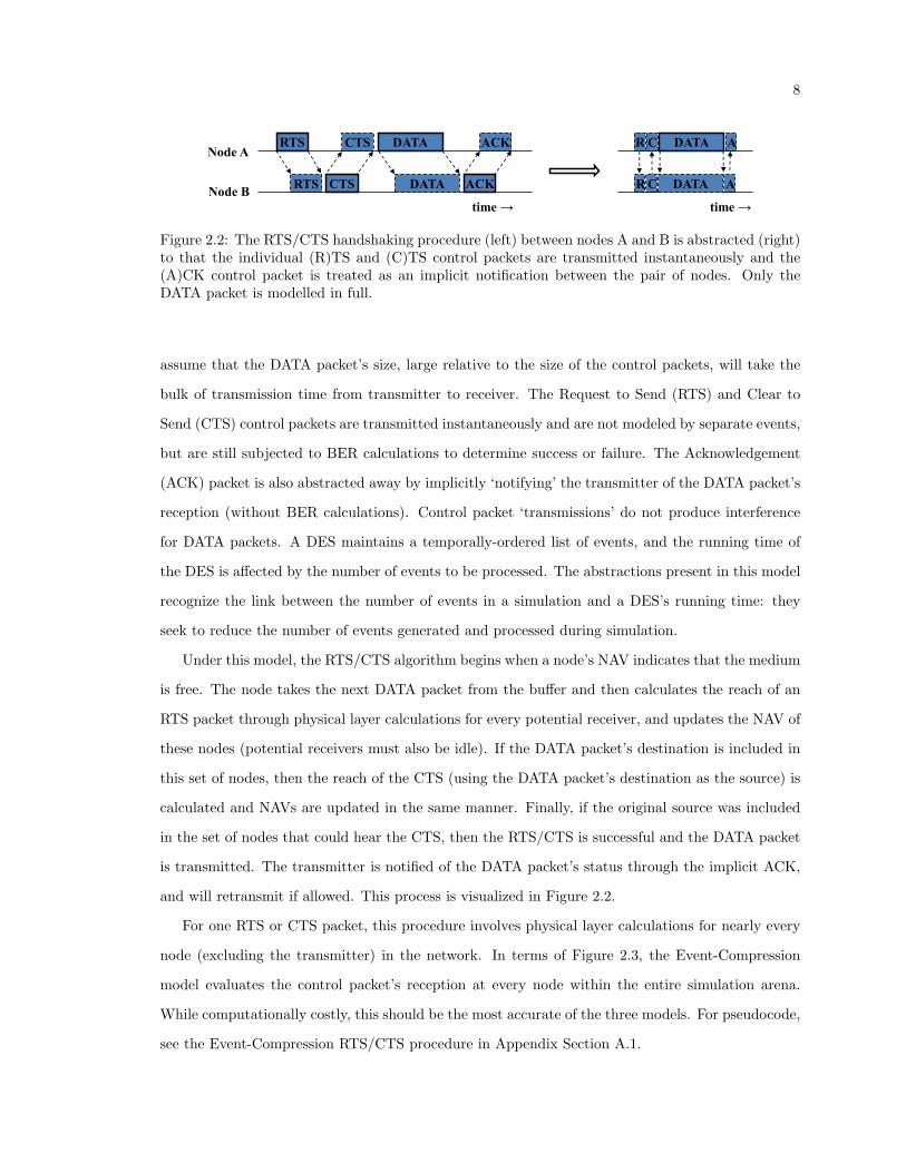
2.2 The abstracted RTS/CTS handshaking procedure between two nodes. . . . . . . . . . . . . . . . . . . . . . . 8
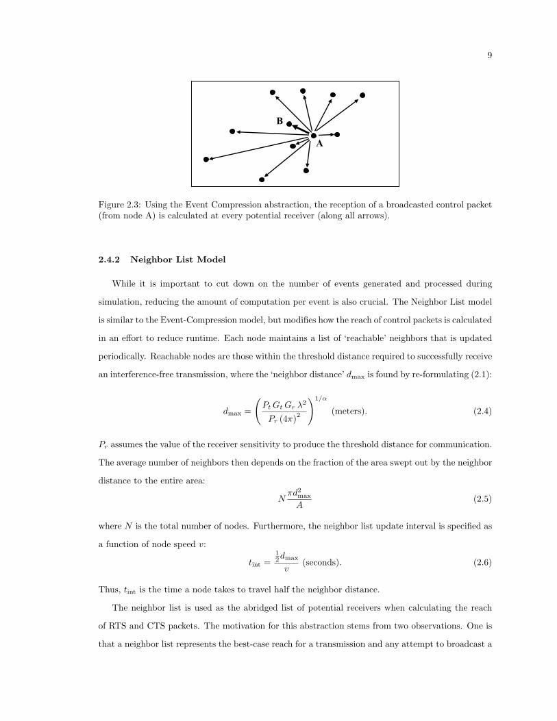
2.3 Using the Event Compression abstraction, the reception of a broadcasted control packet(from node A) is calculated at every potential receiver (along all arrows). . . . . . . . . . . . . . . . . . . 9
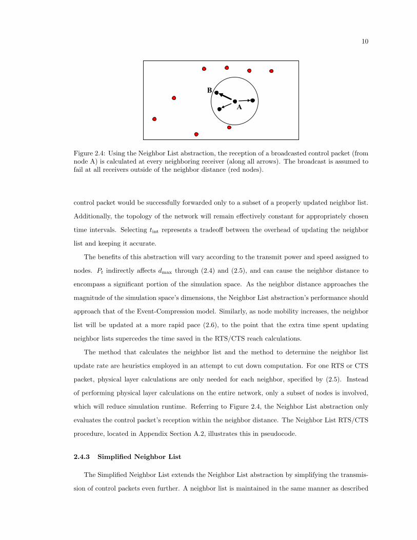
2.4 Using the Neighbor List abstraction, the reception of a broadcasted control packet (fromnode A) is calculated at every neighboring receiver (along all arrows). The broadcast isassumed to fail at all receivers outside of the neighbor distance (red nodes). . . . . . . . . . . . . . . . 10
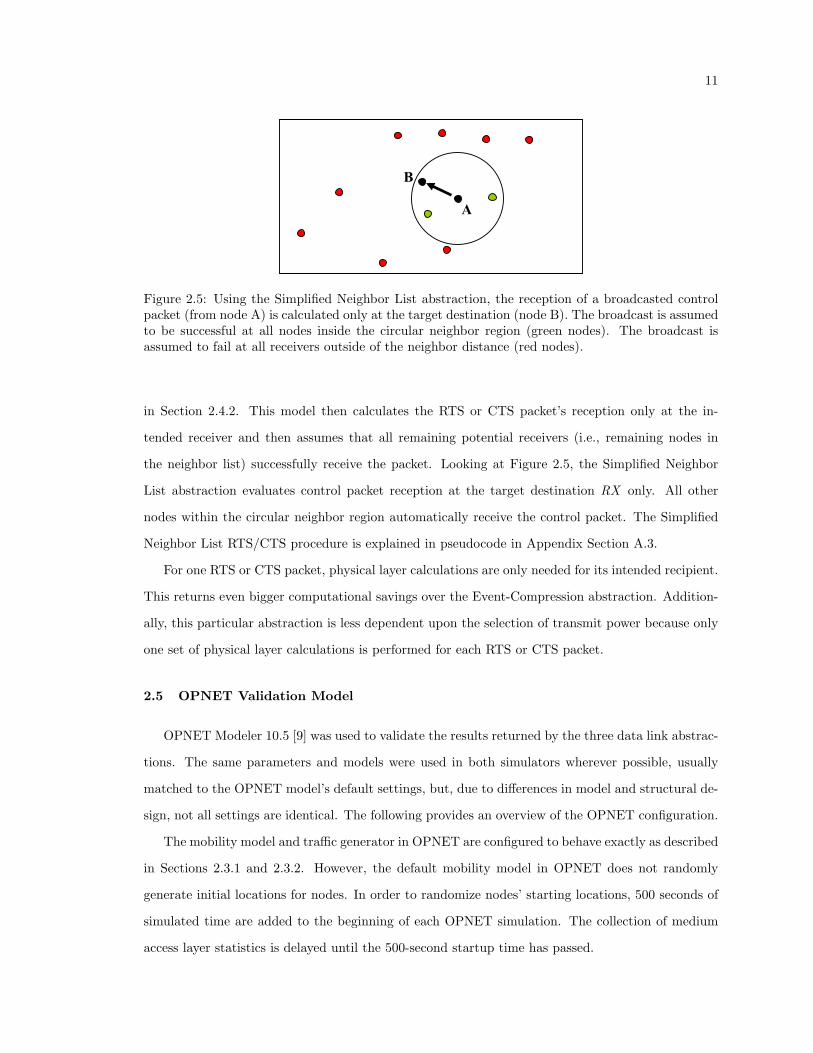
2.5 Using the Simplified Neighbor List abstraction, the reception of a broadcasted controlpacket (from node A) is calculated only at the target destination (node B). The broadcastis assumed to be successful at all nodes inside the circular neighbor region (green nodes).The broadcast is assumed to fail at all receivers outside of the neighbor distance (rednodes). . . . . . . . . . . . . . . . . . . . . . . . . . . . . . . . . . . . . . . . . . . . . . . . . . . . . . . . . . . . . . . . . . . . . . . . . . . . . . . . . . . . . . . . . . . . . 11
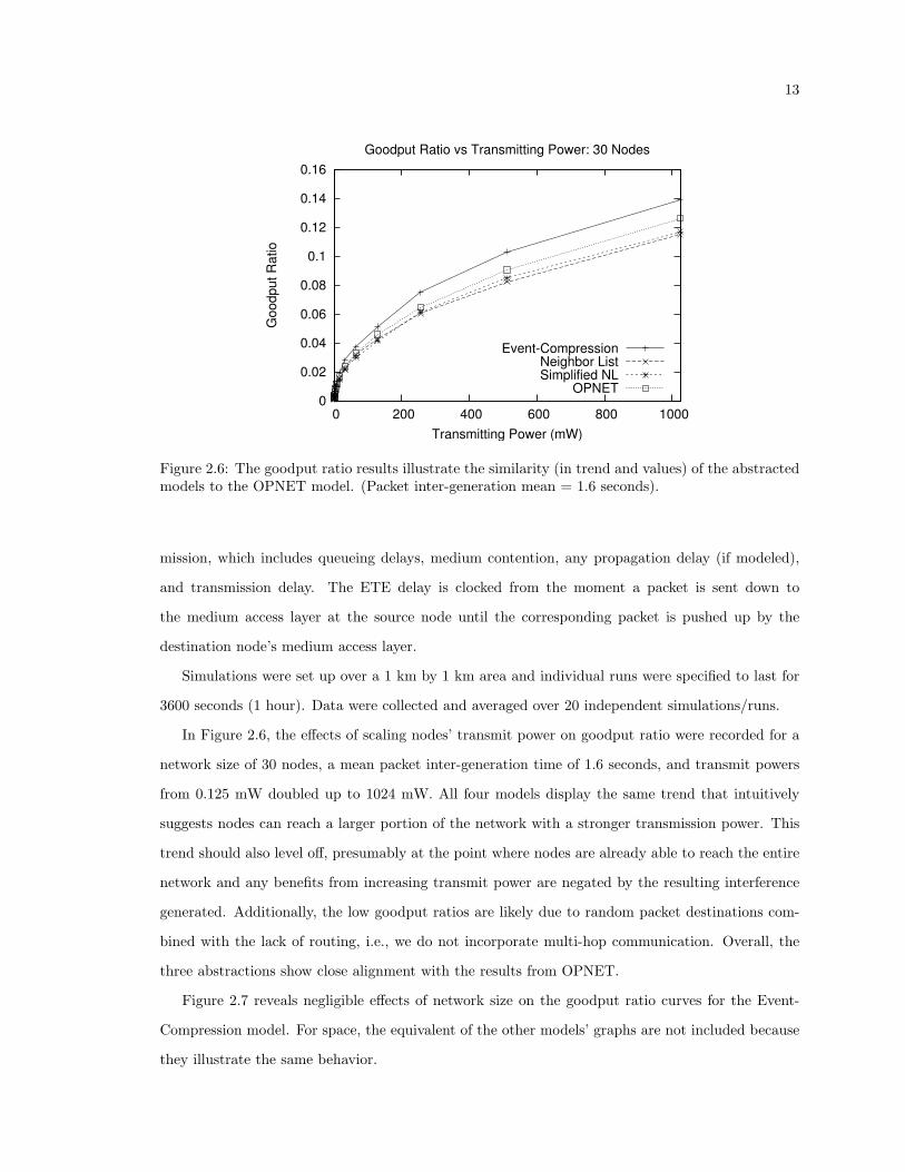
2.6 The goodput ratio results illustrate the similarity (in trend and values) of the abstractedmodels to the OPNET model. (Packet inter-generation mean = 1.6 seconds).. . . . . . . . . . . . . . 13
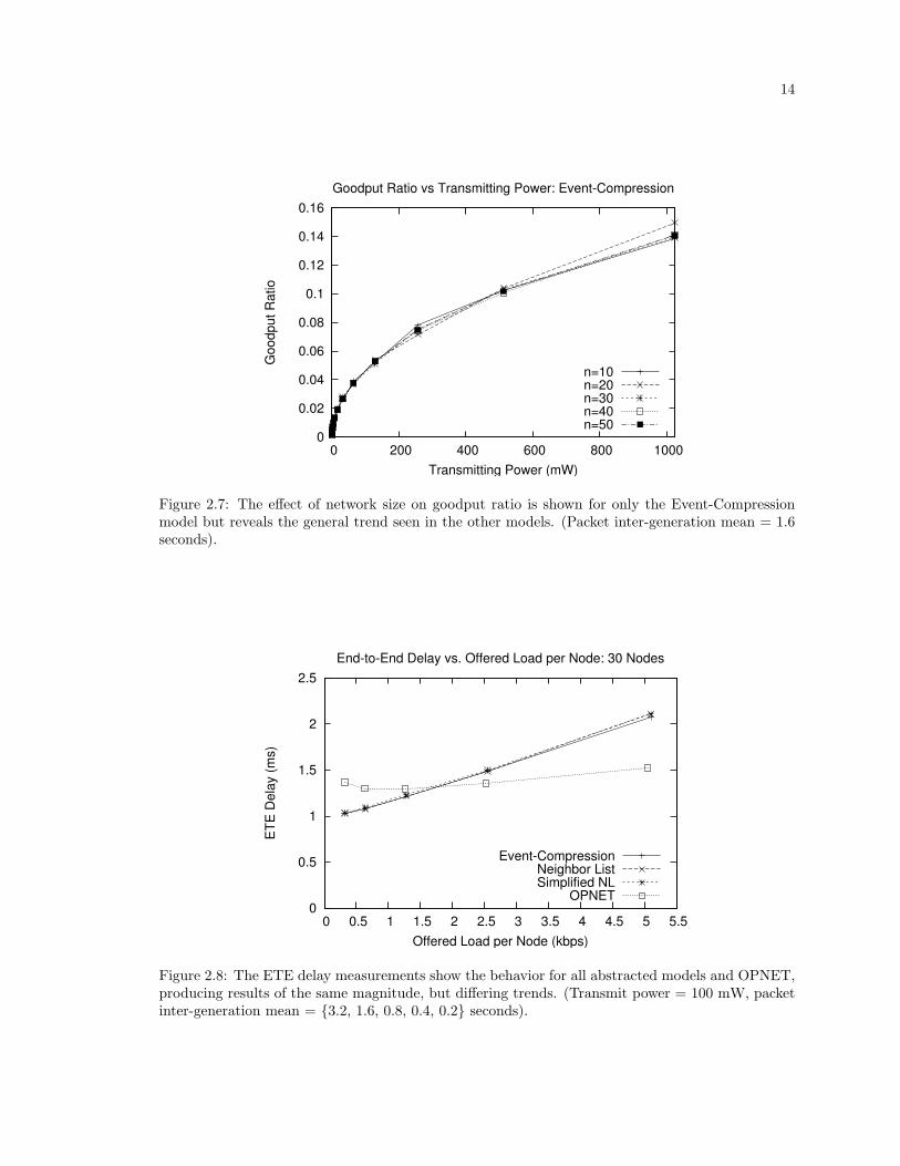
2.7 The effect of network size on goodput ratio is shown for only the Event-Compressionmodel but reveals the general trend seen in the other models. (Packet inter-generationmean = 1.6 seconds).. . . . . . . . . . . . . . . . . . . . . . . . . . . . . . . . . . . . . . . . . . . . . . . . . . . . . . . . . . . . . . . . . . . . . . . . . . . . . 14
2.8 The ETE delay measurements show the behavior for all abstracted models and OPNET,producing results of the same magnitude, but differing trends. (Transmit power = 100mW, packet inter-generation mean = {3.2, 1.6, 0.8, 0.4, 0.2} seconds). . . . . . . . . . . . . . . . . . . . . . 14
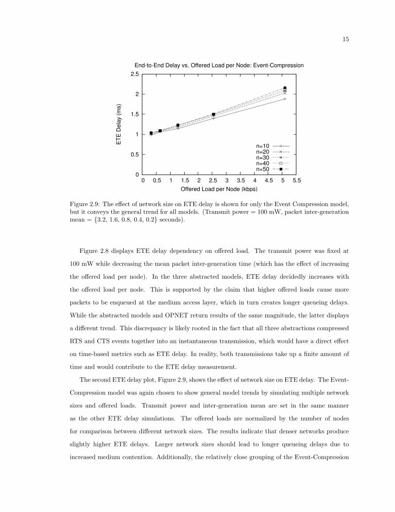
2.9 The effect of network size on ETE delay is shown for only the Event Compression model,but it conveys the general trend for all models. (Transmit power = 100 mW, packetinter-generation mean = {3.2, 1.6, 0.8, 0.4, 0.2} seconds). . . . . . . . . . . . . . . . . . . . . . . . . . . . . . . . . . . . . 15
2.10 The run-time scaling of each model is illustrated. Runtimes are normalized by theirrespective 10-node simulation runtime. (Packet inter-generation mean = 3.2 seconds). . . . . 16
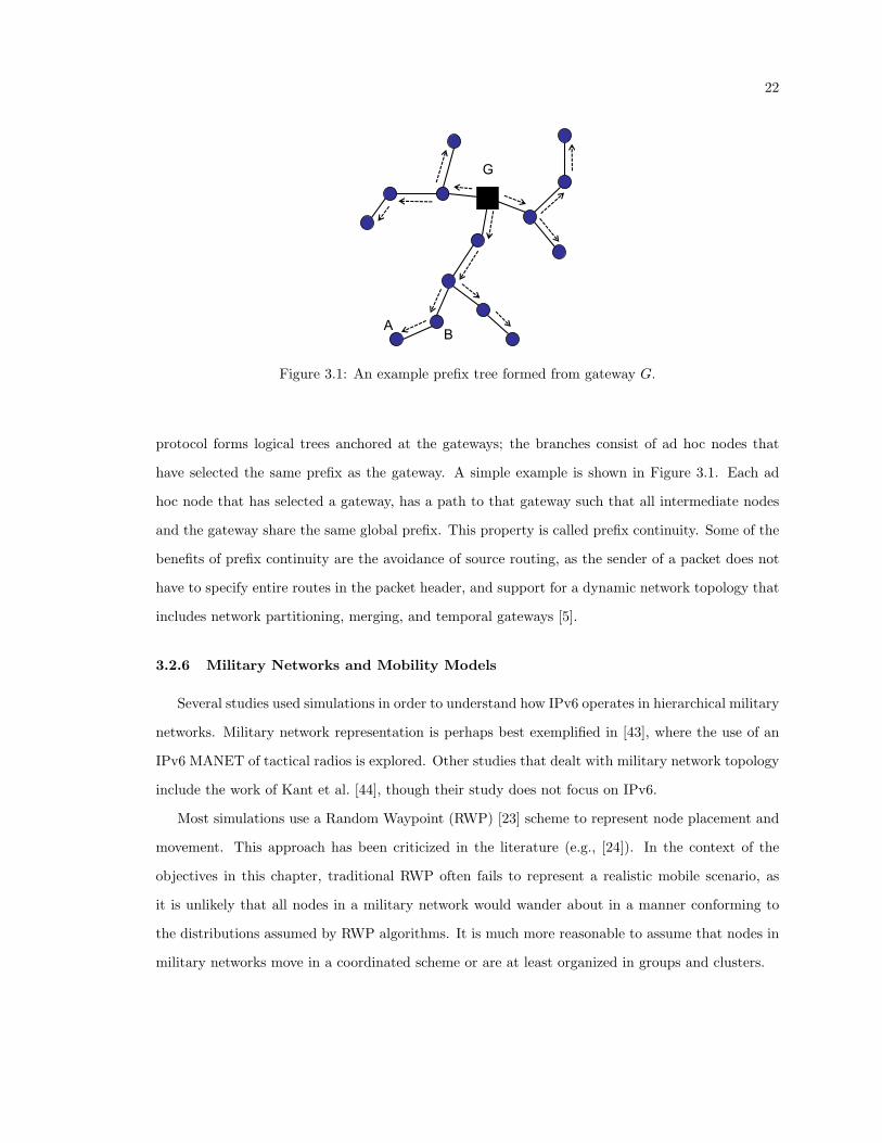
3.1 An example prefix tree formed from gateway G.. . . . . . . . . . . . . . . . . . . . . . . . . . . . . . . . . . . . . . . . . . . . . . . 22
3.2 An example network with two advertising gateways, G1 and G2. . . . . . . . . . . . . . . . . . . . . . . . . . . . . 24
3.3 The logical network topology under consideration. Leaders, denoted by squares, formthe backbone and serve as attachment points for the subordinates, represented as dots. . . 26
3.4 Ad hoc nodes (blue circles) are restricted to choosing waypoints within the vicinity oftheir leader (black square). . . . . . . . . . . . . . . . . . . . . . . . . . . . . . . . . . . . . . . . . . . . . . . . . . . . . . . . . . . . . . . . . . . . . . . 28
3.5 Scenarios I-III are shown from left to right. . . . . . . . . . . . . . . . . . . . . . . . . . . . . . . . . . . . . . . . . . . . . . . . . . . . . 30
3.6 Total autoconfiguration time plotted against the number of ad hoc nodes for varyinggroup mobility parameter values. At the plotted scale, the curve for xy var = 250 liesvery close to the horizontal axis and is not visible. . . . . . . . . . . . . . . . . . . . . . . . . . . . . . . . . . . . . . . . . . . . . 32

v
3.7 Autoconfiguration overhead shown versus the number of ad hoc nodes for varying groupmobility parameter values. . . . . . . . . . . . . . . . . . . . . . . . . . . . . . . . . . . . . . . . . . . . . . . . . . . . . . . . . . . . . . . . . . . . . . . . 33
3.8 Average prefix hold time per node plotted against the number of ad hoc nodes for varyinggroup mobility parameter values. . . . . . . . . . . . . . . . . . . . . . . . . . . . . . . . . . . . . . . . . . . . . . . . . . . . . . . . . . . . . . . . 33
3.9 For a fixed cluster area size (xy var), adding more ad hoc nodes (Nah, circles) promoteslonger logical prefix branches. . . . . . . . . . . . . . . . . . . . . . . . . . . . . . . . . . . . . . . . . . . . . . . . . . . . . . . . . . . . . . . . . . . . 34
3.10 For a fixed number of ad hoc nodes (Nah, circles), increasing the cluster area size (xy var,dashed box) promotes longer logical prefix branches until the network becomes too sparse. 35
3.11 Percentage of time without a prefix per node plotted against various node densities. . . . . . . 36
3.12 Number of prefix updates (left axis) and prefix changes (right axis) versus the number ofmobile gateways. . . . . . . . . . . . . . . . . . . . . . . . . . . . . . . . . . . . . . . . . . . . . . . . . . . . . . . . . . . . . . . . . . . . . . . . . . . . . . . . . . 37
4.1 Traditional Point-to-Point network consisting of two routers. . . . . . . . . . . . . . . . . . . . . . . . . . . . . . . . . 44
4.2 Example Broadcast network with four routers and one Ethernet switch. . . . . . . . . . . . . . . . . . . . . 44
4.3 Example Non-Broadcast Multiple-Access network showing only logical connections. . . . . . . . 45
4.4 Example Point-to-MultiPoint network showing only logical connections. . . . . . . . . . . . . . . . . . . . . 45
4.5 Example network topology using MANET Designated Routers . . . . . . . . . . . . . . . . . . . . . . . . . . . . . . 47
4.6 Link LSA suppression in emulation testbed, generated from Wireshark packet trace. . . . . . . 50
4.7 Overhead differences between OPNET PTP and PTMP interfaces. . . . . . . . . . . . . . . . . . . . . . . . . . 55
4.8 Overhead differences between OPNET radio pipeline stage configurations. . . . . . . . . . . . . . . . . . 56
4.9 Packet generation rate differences between OPNET radio pipeline stage configurations.. . . 57
4.10 Overhead differences between OPNET and emulation testbed MANET (MDR) interface. 58
4.11 Packet generation rate differences between OPNET and emulation testbed MANET(MDR) interface. . . . . . . . . . . . . . . . . . . . . . . . . . . . . . . . . . . . . . . . . . . . . . . . . . . . . . . . . . . . . . . . . . . . . . . . . . . . . . . . . . 58
4.12 OSPFv3 overhead reported for several simulation and emulation environment configura-tions. . . . . . . . . . . . . . . . . . . . . . . . . . . . . . . . . . . . . . . . . . . . . . . . . . . . . . . . . . . . . . . . . . . . . . . . . . . . . . . . . . . . . . . . . . . . . . . 59
4.13 Scaling to larger networks with simulation. . . . . . . . . . . . . . . . . . . . . . . . . . . . . . . . . . . . . . . . . . . . . . . . . . . . . 60

vi
List of Tables
4.1 OSPFv3 Routing Parameters . . . . . . . . . . . . . . . . . . . . . . . . . . . . . . . . . . . . . . . . . . . . . . . . . . . . . . . . . . . . . . . . . . . . 54
4.2 OPNET Percent Error Relative to Emulation Testbed Measurements . . . . . . . . . . . . . . . . . . . . . . . 60
vii
List of Acronyms
AA Addressing Agent.
ACK Acknowledgement.
AODV Ad hoc On-Demand Distance Vector.
ATM Asynchronous Transfer Mode.
BDR Backup Designated Router.
BER Bit Error Rate.
BIDIR Bi-directional.
BMDR Backup MANET Designated Router.
CTS Clear to Send.
DAD Duplicate Address Detection.
DbDesc Database Description.
DCF Distributed Coordination Function.
DES Discrete Event Simulator.
DPSK Differential Phase Shift Keying.
DR Designated Router.
DSDV Destination-Sequenced Distance Vector.
DSSS Direct-Sequence Spread Spectrum.
ETE End-to-End.
FTP File Transfer Protocol.
GW INFO Gateway Information.
HCQA Hybrid Centralized Query-based Autoconfiguration.
IEEE Institute of Electrical and Electronics Engineers.
viii
IETF Internet Engineering Task Force.
IP Internet Protocol.
IPv6 Internet Protocol version 6.
J&N Jelger & Noel.
LSA Link State Advertisement.
LSAck Link State Acknowledgement.
LSReq Link State Request.
LSU Link State Update.
MAC Medium Access Control.
MANET Mobile Ad hoc Network.
MDR MANET Designated Router.
MPR Multipoint Relay.
NAV Network Allocation Vector.
NBMA Non-Broadcast Multiple Access.
OLSR Optimized Link State Routing.
OR Overlapping Relays.
OSPF Open Shortest Path First.
OSPFv3 Open Shortest Path First version 3.
PACMAN Passive AutoConfiguration for Mobile Ad hoc Networks.
PDAD Passive DAD.
PTMP Point-to-Multipoint.
PTP Point-to-Point.
QDAD Query-based DAD.
ix
R-OSPF Radio-OSPF.
RFC Request for Comments.
RTS Request to Send.
RTS/CTS Request to Send/Clear to Send.
RWP Random Waypoint.
SI-CDS Source Independent Connected Dominating Set.
SINR Signal to Interference and Noise Ratio.
UDP User Datagram Protocol.
VLAN Virtual Local Area Network.
WDAD Weak DAD.
WLAN Wireless Local Area Network.
x
Abstract
Topics on Modelling and Simulation of Wireless Networking Protocols
Jeffrey W. Wildman IIAdvisors:
Steven Weber, Ph.D.Moshe Kam, Ph.D., P.E.
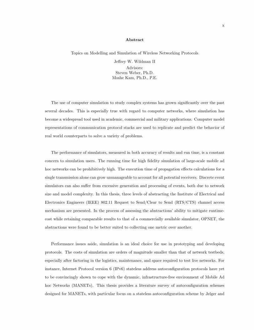
The use of computer simulation to study complex systems has grown significantly over the past
several decades. This is especially true with regard to computer networks, where simulation has
become a widespread tool used in academic, commercial and military applications. Computer model
representations of communication protocol stacks are used to replicate and predict the behavior of
real world counterparts to solve a variety of problems.
The performance of simulators, measured in both accuracy of results and run time, is a constant
concern to simulation users. The running time for high fidelity simulation of large-scale mobile ad
hoc networks can be prohibitively high. The execution time of propagation effects calculations for a
single transmission alone can grow unmanageable to account for all potential receivers. Discrete event
simulators can also suffer from excessive generation and processing of events, both due to network
size and model complexity. In this thesis, three levels of abstracting the Institute of Electrical and
Electronics Engineers (IEEE) 802.11 Request to Send/Clear to Send (RTS/CTS) channel access
mechanism are presented. In the process of assessing the abstractions’ ability to mitigate runtime-
cost while retaining comparable results to that of a commercially available simulator, OPNET, the
abstractions were found to be better suited to collecting one metric over another.
Performance issues aside, simulation is an ideal choice for use in prototyping and developing
protocols. The costs of simulation are orders of magnitude smaller than that of network testbeds,
especially after factoring in the logistics, maintenance, and space required to test live networks. For
instance, Internet Protocol version 6 (IPv6) stateless address autoconfiguration protocols have yet
to be convincingly shown to cope with the dynamic, infrastructure-free environment of Mobile Ad
hoc Networks (MANETs). This thesis provides a literature survey of autoconfiguration schemes
designed for MANETs, with particular focus on a stateless autoconfiguration scheme by Jelger and
xi
Noel (SECON 2005). The selected scheme provides globally routable IPv6 prefixes to a MANET
attached to the Internet via gateways. Using OPNET simulation, the Jelger-Noel scheme is examined
with new cluster mobility models, added gateway mobility, and varied network sizes. Performance of
the Jelger-Noel scheme, derived from overhead, autoconfiguration time and prefix stability metrics,
was found to be highly dependent on network density, and suggested further refinement before
deployment.
Finally, in cases where a network testbed is used to test protocols, it is still advantageous to
run simulations in parallel. While testbeds can help expose design flaws due to code or hardware
differences, discrete event simulation environments can offer extensive debugging capabilities and
event control. The two tools provide independent methods of validating the performance of protocols,
as well as providing useful feedback on correct protocol implementation and configuration. This
thesis presents the Open Shortest Path First (OSPF) routing protocol and its MANET extensions
as candidate protocols to test in simulated and emulated MANETs. The measured OSPF overhead
from both environments was used as a benchmark to construct equivalent MANET representations
and protocol configuration, made particularly challenging due to the wired nature of the emulation
testbed. While attempting to duplicate and validate results of a previous OSPF study, limitations
of the simulated implementation of OSPF were revealed.

1
1. Introduction
The use of computer simulation to study complex systems has grown significantly over the past
several decades. This is especially true with regard to computer networks, where simulation has
become a widespread tool used in academic, commercial and military applications. Computer model
representations of communication protocol stacks are used to replicate and predict the behavior of
real world counterparts to solve a variety of problems.
The popularity of simulation stems from the fact that computing power continually becomes
faster and cheaper. The cost of simulation hardware and software has become orders of magnitude
smaller than that of network testbeds, especially for large networks. Simulation also avoids the
logistics, maintenance, and space required to test live networks, such as mobile ad hoc networks with
complex, coordinated movement patterns [1]. Often, simulation is used to answer queries about the
performance of a network prior to making investments in hardware and bandwidth. Simulations
can advise on the minimal set of hardware required to provide a desired quality of service; examples
include expanding commercial networks to support additional offices, overprovisioning by Internet
Service Providers, and determining buffer sizes for streaming media over the Internet.
Several features of computer simulation prove to be extremely beneficial for research and devel-
opment of new and existing network protocols. Discrete event simulation environments can offer
extensive debugging capabilities and event control, such as the ability of stopping time and stepping
through events to examine the states and interaction of model internals. Reproducible simulation
runs, controlled by a random seed, allow the re-creation of particular events of interest in proto-
col operation. Students can also take advantage of all of these characteristics of simulation in the
classroom to learn more about computer networking.
However, the performance of simulations, both in accuracy of results and run time, are a constant
concern of the users of such software. Simulators are not bound to a 1:1 ‘real-time’ run time, which
can result in wildly varying speedup or slowdown factors. The run time is largely dependent on the
fidelity of the models and the number of devices being simulated [2]. In cases where estimates of
network performance are time-critical, such as military deployments or natural disaster responses,
the simulated networks are likely to be very large and the simulation results must be extremely
accurate. Additionally, simulation of a network may not provide certain vital information about the
‘production model’. Differences in protocol stack implementation and hardware may hide software
2
bugs from view until testbeds are employed [1, 3].
The combined benefits and drawbacks of computer network simulation provide a large variety of
research problems to the research community, both to employ simulation to solve problems and to
resolve problems with the simulation process itself. This thesis is comprised of three case studies that
a) highlight issues affecting the use of simulation, as well as b) detail ways of applying simulation
to the study of wireless networking protocols.
Chapter 2 examines the tradeoff between running time and model fidelity for large-scale Mo-
bile Ad hoc Network (MANET) simulations. Three levels of abstracting the Institute of Electrical
and Electronics Engineers (IEEE) 802.11 Request to Send/Clear to Send (RTS/CTS) channel ac-
cess mechanism are presented and simulated against a commercially available network simulator,
OPNET. The abstractions are assessed by their ability to mitigate runtime cost while retaining
comparable results to the commercial simulator. The abstractions are found to be better suited to
collecting some metrics than others. This work was presented at MILCOM 2006 [4].
Chapter 3 examines the feasibility of a new protocol via simulation. A literature survey of
autoconfiguration schemes designed for MANETs is provided, with particular focus on a stateless
autoconfiguration scheme by Jelger and Noel (SECON 2005) [5]. The selected scheme provides
globally routable Internet Protocol version 6 (IPv6) prefixes to a MANET attached to the Internet
via gateways. Using OPNET simulation, the Jelger-Noel scheme is examined with new cluster
mobility models, gateway mobility, and varied network sizes. Performance of the Jelger-Noel scheme,
measured from overhead, autoconfiguration time and prefix stability metrics, is found to be highly
dependent on network density, and suggests further refinement before deployment. This work was
presented at MILCOM 2007 [6].
In Chapter 4, simulations are used to cross-validate an emulation testbed running the Open
Shortest Path First (OSPF) routing protocol and its MANET Designated Router (MDR) exten-
sion. The measured OSPF overhead from both environments is used as a benchmark to construct
equivalent MANET representations and protocol configuration, made particularly challenging due
to the wired nature of the emulation testbed. Compromises are struck between the emulation and
simulation environments to bring routing overhead and packet rate measurements within acceptable
levels between the environments. While attempting to duplicate and validate results of a previous
OSPF study, limitations of the simulated implementation of OSPF are revealed. Specifics on the
emulation testbed configuration were presented at MILCOM 2008 [7].
Finally, Chapter 5 summarizes each of the three studies and highlights important findings.
3
2. RTS-CTS Abstractions
2.1 Introduction
Meaningful simulation of ad hoc wireless networks is a time-intensive task and reducing the
execution time is important, particularly when planning networks for use in military operations.
For such simulations, the desired scale can range from hundreds to thousands of radios and the
results are often needed within hours or days. For large ad hoc networks, the most computation-
intensive tasks in simulation are computing interference and determining which receivers are in range
of a transmitter. In both cases, O(N2) physical layer calculations are required for a wireless system
of N nodes, which scales poorly.
There are several proposals to improve the running time necessary to calculate the inter-nodal
interference. Naoumov and Gross [8] introduce a 3-dimensional array of pointers to nodes ordered by
x- and y-coordinates, which they use to reduce the amount of space searched for nodes within range
of the transmitter. A similar approach is employed in this study but, while [8] focuses on reducing the
number of potential interferers, we focus instead on reducing the number of calculations necessary
to determine the set of potential receivers. Several techniques, or abstractions, are presented to
improve scalability and decrease running time of an Institute of Electrical and Electronics Engineers
(IEEE) 802.11 wireless model while achieving equivalent simulation results to that of a commercially
available simulator, OPNET. In the process of assessing the abstractions’ ability to mitigate runtime
cost, the abstractions were found to be better suited to collecting some metrics over others.
The rest of this chapter is organized as follows. Section 2.2 contains a survey of related research.
Section 2.3 presents models and the parameters of the custom-built simulator running abstractions
of the IEEE 802.11 protocol. Section 2.4 describes the proposed abstraction models. Section 2.5
introduces the validation method used and highlights the differences between the custom simulator
and OPNET Modeler [9]. In Section 2.6, results gathered from both simulators are compared and
discussed. Section 2.7 concludes the chapter and suggests possible avenues of future work on this
topic.
4
2.2 Survey of Literature on Simulation Performance
Previous studies of mobile network simulation suggest two primary methods for improving simu-
lation performance: parallel programming (assuming multiple processors are available) [10–12] and
model abstraction [1,13]. Each of these methods involves certain trade-offs. A parallelized approach
may scale well without losing accuracy but at a high cost in computing resources, while abstraction
improves execution time but may sacrifice some degree of accuracy. Additionally, these methods are
not mutually exclusive and may be employed together.
The physics of radio transmission introduce challenges to simulation not present with wired
networks [14]. The one-to-many broadcast nature of wireless transmissions is fundamentally different
than one-to-one communication in wired networks. In a radio-connected network, the distances at
which a transmission can be successfully received and at which a transmission may cause interference
may be different [8]. Takai, et al. [15] provide a good description of several approaches to modeling
the physical layer and the consequences of choosing one model over another. A simulation is a
simplification of a real-world system [16] and careful consideration must be given to the details
omitted. A good summary of the issues involved is given by Heidemann, et al. [14]. Cavin, et al. [17]
discuss issues relating to the accuracy of mobile ad hoc network simulators and ways of analyzing
the results.
A highly detailed network model often greatly reduces scalability, meaning the model is infeasible
for simulating large networks. However, less detailed models can reduce the reliability of the results.
Blum, et al. [2] introduce a ‘dual mode’ approach that dynamically switches between detailed sim-
ulation models and abstractions depending on network conditions. Naoumov and Gross [8] reduce
execution time by exploiting the probability that nodes will be spread throughout the modeled space.
Perrone and Nicol [18] use the Barnes-Hut (N-body) algorithm based on the observation that the
gravitational pull between objects in astrophysical models is similar to signal attenuation models
of wireless models in that both decay polynomially with distance. The amount of detail that can
safely be abstracted out depends on what network behavior is being studied, as discussed by Liu,
et al. [19] and by Zhong and Rabaey [20]. Golmie, et al. [21] and Heindl and German [22] present
approaches to modeling the IEEE 802.11 protocol.
5
2.3 Custom-built Simulator Models
A packet-based, Discrete Event Simulator (DES) was developed for the purposes of this study.
The simulator includes models at the physical, medium access, and application layers in addition to
mobility models. Nodes are all modeled homogeneously and are described by their mobility, traffic
generation, and transmission protocol.
2.3.1 Mobility
A Random Waypoint (RWP) [23] model captures the network’s dynamic topology. Initial node
positions are chosen independently and uniformly at random from the entire 1 km by 1 km simulation
space. Nodes travel at a constant speed of 1 m/s, and choose destinations (waypoints) uniformly
from the arena without a ‘pause time’ between waypoints. This movement model was selected both
for simplicity and to avoid the transient behavior inherent in certain RWP models in which nodes
experience a ‘slowdown’ over time [24].
2.3.2 Traffic
The application layer consists of a basic source and sink. Nodes generate packets for the dura-
tion of the simulation. Each node’s packet generation times form an independent and identically
distributed Poisson point process. Packet sizes are chosen from an exponential distribution with a
mean of 128 bytes. The destination of each packet is picked uniformly from the full set of nodes.
2.3.3 Transmission
At the physical layer, the Friis transmission equation governs signal attenuation:
P i,jr (t) =P it (t)GtGr λ
2
(4π)2 dαi,j(t)(mW) (2.1)
where P i,jr (t) is the received power at node j from transmitting node i at time t, P it (t) is the
transmitted power at node i, and di,j(t) is the distance between transmitter i and receiver j (in
meters). Transmitter and receiver antenna gains, Gt and Gr, are assumed to be isotropic and are
set to 2. The wavelength λ (in meters) is derived from the first IEEE 802.11b Direct-Sequence
Spread Spectrum (DSSS) channel’s center-frequency of 2.412 GHz. The pathloss constant α is set
to 4 to model stronger signal attenuation than free space [25].
6
Interference power measured at node j at time t, given a desired transmission from node i, is
given by:
Ij(t) =∑
k∈T (t)\i
P k,jr (t) (mW) (2.2)
where T (t) is the set of all transmitting nodes at time t.
A Bit Error Rate (BER) model is used in addition to (2.1) and (2.2) to evaluate a signal’s
likelihood for success. It maps received power and interference levels to a BER assuming a Differential
Phase Shift Keying (DPSK) modulation scheme:
BER = 0.5 exp(
−EbNo + I/R
). (2.3)
Here, R is the data rate, Eb is the received energy per bit (Pr/R), I/R is the interference energy per
bit, and No accounts for noise from the environment and the receiver’s electronics. No is derived from
an achievable BER at a given receiver sensitivity and data rate. At 11 Mbps, nodes were assumed
to experience a BER of 10−4 at a receiver sensitivity of Pr = −95 dBm. These parameters assume
zero interference (I = 0 mW) which allows (2.3) to be rearranged to solve for No = 3.38 × 10⁻¹⁸
mW. Use of (2.3) during simulation is then carried out for a calculated received power Pr, aggregate
interference power I, and the pre-solved No.
Transmission success is determined by modeling the number of bit errors nerror incurred during
packet transmission as a binomial random variable nerror ∼ B(n, p) with n total bits and a BER
of p. Since error correction is not modeled, a single error will result in a dropped packet. The
probability of packet success equates to generating nerror = 0 bit errors and assuming each bit in a
packet is in error independently, the packet success rate is (1− p)n.
The simulator maintains a network-wide list of transmitting packets. The list is updated dynam-
ically as packets start and finish transmitting. Whenever a packet is added, the BER is recalculated
for every packet on the list to reflect new interference conditions. Each packet’s new BER is then
used to predict the number of errors over the entire length of the packet. If any errors are predicted,
the transmission attempt corresponding to the packet is marked as failed. Once a packet is marked
as failed, it remains as such. Figure 2.1 shows a sample trace of packet transmissions that begin at
times t1, t2, and t4. Over the course of the sample packet timing chart, physical layer calculations
are performed at times t1 and t2 for packet 1, times t2, t3, and t4 for packet 2, and times t4 and t5
for packet 3. Additionally, transmission times do not include propagation delay.

7
t i m e
packet 1
packet 2
packet 3
t 1 t 2 t 3 t 4 t 5 t 6
Figure 2.1: Example timing chart of packet transmissions.
2.4 IEEE 802.11 Model Abstractions
The custom-built simulator’s medium access layer contains three abstractions of the IEEE 802.11
Standard. Sources used in implementation include [25] and [26]. Given the infrastructureless nature
of ad hoc networks, all abstractions use the Distributed Coordination Function (DCF) to handle
media access control. A Network Allocation Vector (NAV) is used in conjunction with binary expo-
nential back-off to determine medium access. Physical carrier sensing (via beaconing) is not simu-
lated, but virtual carrier sensing is accomplished by the Request to Send/Clear to Send (RTS/CTS)
mechanism. Every packet initiates an RTS/CTS sequence, regardless of its size. Packets are not
fragmented, and large packets are dropped immediately upon reaching the datalink layer. Packets’
sizes are increased by 292 bytes at the medium access layer to account for headers and physical
layer overhead (to match OPNET), which results in an overall mean packet size of 128 + 292 bytes.
Packet queues are maintained at each node with a maximum size of 32 KB of simulated data, and
packets are dropped after four transmission attempts. The exact implementation of RTS/CTS for
each model differs, as each model adds an additional degree of abstraction to the previous one. Note
that nodes use only one of the abstractions during any given simulation to maintain homogeneity.
The remainder of this section discusses the three developed abstractions, the Event-Compression,
Neighbor List, and Simplified Neighbor List models.
2.4.1 Event-Compression Model
Of the three abstractions to be presented, the Event-Compression model strays the least from
the validation model (discussed in Section 2.5) in terms of implementation. Specifically, its most
significant abstractions are the use of a collapsed-RTS/CTS and implicit acknowledgement. Both
8
RTS
RTS
Node A
Node BCTS
CTS
ACK
ACKDATA
DATA
R
R C
C
A
ADATA
DATA
time → time →
Figure 2.2: The RTS/CTS handshaking procedure (left) between nodes A and B is abstracted (right)to that the individual (R)TS and (C)TS control packets are transmitted instantaneously and the(A)CK control packet is treated as an implicit notification between the pair of nodes. Only theDATA packet is modelled in full.
assume that the DATA packet’s size, large relative to the size of the control packets, will take the
bulk of transmission time from transmitter to receiver. The Request to Send (RTS) and Clear to
Send (CTS) control packets are transmitted instantaneously and are not modeled by separate events,
but are still subjected to BER calculations to determine success or failure. The Acknowledgement
(ACK) packet is also abstracted away by implicitly ‘notifying’ the transmitter of the DATA packet’s
reception (without BER calculations). Control packet ‘transmissions’ do not produce interference
for DATA packets. A DES maintains a temporally-ordered list of events, and the running time of
the DES is affected by the number of events to be processed. The abstractions present in this model
recognize the link between the number of events in a simulation and a DES’s running time: they
seek to reduce the number of events generated and processed during simulation.
Under this model, the RTS/CTS algorithm begins when a node’s NAV indicates that the medium
is free. The node takes the next DATA packet from the buffer and then calculates the reach of an
RTS packet through physical layer calculations for every potential receiver, and updates the NAV of
these nodes (potential receivers must also be idle). If the DATA packet’s destination is included in
this set of nodes, then the reach of the CTS (using the DATA packet’s destination as the source) is
calculated and NAVs are updated in the same manner. Finally, if the original source was included
in the set of nodes that could hear the CTS, then the RTS/CTS is successful and the DATA packet
is transmitted. The transmitter is notified of the DATA packet’s status through the implicit ACK,
and will retransmit if allowed. This process is visualized in Figure 2.2.
For one RTS or CTS packet, this procedure involves physical layer calculations for nearly every
node (excluding the transmitter) in the network. In terms of Figure 2.3, the Event-Compression
model evaluates the control packet’s reception at every node within the entire simulation arena.
While computationally costly, this should be the most accurate of the three models. For pseudocode,
see the Event-Compression RTS/CTS procedure in Appendix Section A.1.
9
A
B
Figure 2.3: Using the Event Compression abstraction, the reception of a broadcasted control packet(from node A) is calculated at every potential receiver (along all arrows).
2.4.2 Neighbor List Model
While it is important to cut down on the number of events generated and processed during
simulation, reducing the amount of computation per event is also crucial. The Neighbor List model
is similar to the Event-Compression model, but modifies how the reach of control packets is calculated
in an effort to reduce runtime. Each node maintains a list of ‘reachable’ neighbors that is updated
periodically. Reachable nodes are those within the threshold distance required to successfully receive
an interference-free transmission, where the ‘neighbor distance’ dmax is found by re-formulating (2.1):
dmax =
(PtGtGr λ
2
Pr (4π)2
)1/α
(meters). (2.4)
Pr assumes the value of the receiver sensitivity to produce the threshold distance for communication.
The average number of neighbors then depends on the fraction of the area swept out by the neighbor
distance to the entire area:
Nπd2
max
A(2.5)
where N is the total number of nodes. Furthermore, the neighbor list update interval is specified as
a function of node speed v:
tint =12dmax
v(seconds). (2.6)
Thus, tint is the time a node takes to travel half the neighbor distance.
The neighbor list is used as the abridged list of potential receivers when calculating the reach
of RTS and CTS packets. The motivation for this abstraction stems from two observations. One is
that a neighbor list represents the best-case reach for a transmission and any attempt to broadcast a
10
A
B
Figure 2.4: Using the Neighbor List abstraction, the reception of a broadcasted control packet (fromnode A) is calculated at every neighboring receiver (along all arrows). The broadcast is assumed tofail at all receivers outside of the neighbor distance (red nodes).
control packet would be successfully forwarded only to a subset of a properly updated neighbor list.
Additionally, the topology of the network will remain effectively constant for appropriately chosen
time intervals. Selecting tint represents a tradeoff between the overhead of updating the neighbor
list and keeping it accurate.
The benefits of this abstraction will vary according to the transmit power and speed assigned to
nodes. Pt indirectly affects dmax through (2.4) and (2.5), and can cause the neighbor distance to
encompass a significant portion of the simulation space. As the neighbor distance approaches the
magnitude of the simulation space’s dimensions, the Neighbor List abstraction’s performance should
approach that of the Event-Compression model. Similarly, as node mobility increases, the neighbor
list will be updated at a more rapid pace (2.6), to the point that the extra time spent updating
neighbor lists supercedes the time saved in the RTS/CTS reach calculations.
The method that calculates the neighbor list and the method to determine the neighbor list
update rate are heuristics employed in an attempt to cut down computation. For one RTS or CTS
packet, physical layer calculations are only needed for each neighbor, specified by (2.5). Instead
of performing physical layer calculations on the entire network, only a subset of nodes is involved,
which will reduce simulation runtime. Referring to Figure 2.4, the Neighbor List abstraction only
evaluates the control packet’s reception within the neighbor distance. The Neighbor List RTS/CTS
procedure, located in Appendix Section A.2, illustrates this in pseudocode.
2.4.3 Simplified Neighbor List
The Simplified Neighbor List extends the Neighbor List abstraction by simplifying the transmis-
sion of control packets even further. A neighbor list is maintained in the same manner as described
11
A
B
Figure 2.5: Using the Simplified Neighbor List abstraction, the reception of a broadcasted controlpacket (from node A) is calculated only at the target destination (node B). The broadcast is assumedto be successful at all nodes inside the circular neighbor region (green nodes). The broadcast isassumed to fail at all receivers outside of the neighbor distance (red nodes).
in Section 2.4.2. This model then calculates the RTS or CTS packet’s reception only at the in-
tended receiver and then assumes that all remaining potential receivers (i.e., remaining nodes in
the neighbor list) successfully receive the packet. Looking at Figure 2.5, the Simplified Neighbor
List abstraction evaluates control packet reception at the target destination RX only. All other
nodes within the circular neighbor region automatically receive the control packet. The Simplified
Neighbor List RTS/CTS procedure is explained in pseudocode in Appendix Section A.3.
For one RTS or CTS packet, physical layer calculations are only needed for its intended recipient.
This returns even bigger computational savings over the Event-Compression abstraction. Addition-
ally, this particular abstraction is less dependent upon the selection of transmit power because only
one set of physical layer calculations is performed for each RTS or CTS packet.
2.5 OPNET Validation Model
OPNET Modeler 10.5 [9] was used to validate the results returned by the three data link abstrac-
tions. The same parameters and models were used in both simulators wherever possible, usually
matched to the OPNET model’s default settings, but, due to differences in model and structural de-
sign, not all settings are identical. The following provides an overview of the OPNET configuration.
The mobility model and traffic generator in OPNET are configured to behave exactly as described
in Sections 2.3.1 and 2.3.2. However, the default mobility model in OPNET does not randomly
generate initial locations for nodes. In order to randomize nodes’ starting locations, 500 seconds of
simulated time are added to the beginning of each OPNET simulation. The collection of medium
access layer statistics is delayed until the 500-second startup time has passed.
12
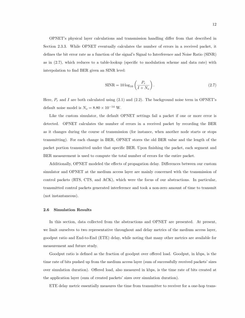
OPNET’s physical layer calculations and transmission handling differ from that described in
Section 2.3.3. While OPNET eventually calculates the number of errors in a received packet, it
defines the bit error rate as a function of the signal’s Signal to Interference and Noise Ratio (SINR)
as in (2.7), which reduces to a table-lookup (specific to modulation scheme and data rate) with
interpolation to find BER given an SINR level:
SINR = 10 log10
(Pr
I +No
). (2.7)
Here, Pr and I are both calculated using (2.1) and (2.2). The background noise term in OPNET’s
default noise model is No = 8.80× 10⁻¹⁴ W.
Like the custom simulator, the default OPNET settings fail a packet if one or more error is
detected. OPNET calculates the number of errors in a received packet by recording the BER
as it changes during the course of transmission (for instance, when another node starts or stops
transmitting). For each change in BER, OPNET stores the old BER value and the length of the
packet portion transmitted under that specific BER. Upon finishing the packet, each segment and
BER measurement is used to compute the total number of errors for the entire packet.
Additionally, OPNET modeled the effects of propagation delay. Differences between our custom
simulator and OPNET at the medium access layer are mainly concerned with the transmission of
control packets (RTS, CTS, and ACK), which were the focus of our abstractions. In particular,
transmitted control packets generated interference and took a non-zero amount of time to transmit
(not instantaneous).
2.6 Simulation Results
In this section, data collected from the abstractions and OPNET are presented. At present,
we limit ourselves to two representative throughout and delay metrics of the medium access layer,
goodput ratio and End-to-End (ETE) delay, while noting that many other metrics are available for
measurement and future study.
Goodput ratio is defined as the fraction of goodput over offered load. Goodput, in kbps, is the
time rate of bits pushed up from the medium access layer (sum of successfully received packets’ sizes
over simulation duration). Offered load, also measured in kbps, is the time rate of bits created at
the application layer (sum of created packets’ sizes over simulation duration).
ETE delay metric essentially measures the time from transmitter to receiver for a one-hop trans-
13
0
0.02
0.04
0.06
0.08
0.1
0.12
0.14
0.16
0 200 400 600 800 1000
Goo
dput
Rat
io
Transmitting Power (mW)
Goodput Ratio vs Transmitting Power: 30 Nodes
Event-CompressionNeighbor ListSimplified NL
OPNET
Figure 2.6: The goodput ratio results illustrate the similarity (in trend and values) of the abstractedmodels to the OPNET model. (Packet inter-generation mean = 1.6 seconds).
mission, which includes queueing delays, medium contention, any propagation delay (if modeled),
and transmission delay. The ETE delay is clocked from the moment a packet is sent down to
the medium access layer at the source node until the corresponding packet is pushed up by the
destination node’s medium access layer.
Simulations were set up over a 1 km by 1 km area and individual runs were specified to last for
3600 seconds (1 hour). Data were collected and averaged over 20 independent simulations/runs.
In Figure 2.6, the effects of scaling nodes’ transmit power on goodput ratio were recorded for a
network size of 30 nodes, a mean packet inter-generation time of 1.6 seconds, and transmit powers
from 0.125 mW doubled up to 1024 mW. All four models display the same trend that intuitively
suggests nodes can reach a larger portion of the network with a stronger transmission power. This
trend should also level off, presumably at the point where nodes are already able to reach the entire
network and any benefits from increasing transmit power are negated by the resulting interference
generated. Additionally, the low goodput ratios are likely due to random packet destinations com-
bined with the lack of routing, i.e., we do not incorporate multi-hop communication. Overall, the
three abstractions show close alignment with the results from OPNET.
Figure 2.7 reveals negligible effects of network size on the goodput ratio curves for the Event-
Compression model. For space, the equivalent of the other models’ graphs are not included because
they illustrate the same behavior.
14
0
0.02
0.04
0.06
0.08
0.1
0.12
0.14
0.16
0 200 400 600 800 1000
Goo
dput
Rat
io
Transmitting Power (mW)
Goodput Ratio vs Transmitting Power: Event-Compression
n=10n=20n=30n=40n=50
Figure 2.7: The effect of network size on goodput ratio is shown for only the Event-Compressionmodel but reveals the general trend seen in the other models. (Packet inter-generation mean = 1.6seconds).
0
0.5
1
1.5
2
2.5
0 0.5 1 1.5 2 2.5 3 3.5 4 4.5 5 5.5
ETE
Dela
y (m
s)
Offered Load per Node (kbps)
End-to-End Delay vs. Offered Load per Node: 30 Nodes
Event-CompressionNeighbor ListSimplified NL
OPNET
Figure 2.8: The ETE delay measurements show the behavior for all abstracted models and OPNET,producing results of the same magnitude, but differing trends. (Transmit power = 100 mW, packetinter-generation mean = {3.2, 1.6, 0.8, 0.4, 0.2} seconds).
15
0
0.5
1
1.5
2
2.5
0 0.5 1 1.5 2 2.5 3 3.5 4 4.5 5 5.5
ETE
Dela
y (m
s)
Offered Load per Node (kbps)
End-to-End Delay vs. Offered Load per Node: Event-Compression
n=10n=20n=30n=40n=50
Figure 2.9: The effect of network size on ETE delay is shown for only the Event Compression model,but it conveys the general trend for all models. (Transmit power = 100 mW, packet inter-generationmean = {3.2, 1.6, 0.8, 0.4, 0.2} seconds).
Figure 2.8 displays ETE delay dependency on offered load. The transmit power was fixed at
100 mW while decreasing the mean packet inter-generation time (which has the effect of increasing
the offered load per node). In the three abstracted models, ETE delay decidedly increases with
the offered load per node. This is supported by the claim that higher offered loads cause more
packets to be enqueued at the medium access layer, which in turn creates longer queueing delays.
While the abstracted models and OPNET return results of the same magnitude, the latter displays
a different trend. This discrepancy is likely rooted in the fact that all three abstractions compressed
RTS and CTS events together into an instantaneous transmission, which would have a direct effect
on time-based metrics such as ETE delay. In reality, both transmissions take up a finite amount of
time and would contribute to the ETE delay measurement.
The second ETE delay plot, Figure 2.9, shows the effect of network size on ETE delay. The Event-
Compression model was again chosen to show general model trends by simulating multiple network
sizes and offered loads. Transmit power and inter-generation mean are set in the same manner
as the other ETE delay simulations. The offered loads are normalized by the number of nodes
for comparison between different network sizes. The results indicate that denser networks produce
slightly higher ETE delays. Larger network sizes should lead to longer queueing delays due to
increased medium contention. Additionally, the relatively close grouping of the Event-Compression

16
0
5
10
15
20
25
30
0 10 20 30 40 50 60
Fact
or
Number of Nodes
Model Scaling vs Number of Nodes
Event-CompressionNeighbor ListSimplified NL
OPNET
Figure 2.10: The run-time scaling of each model is illustrated. Runtimes are normalized by theirrespective 10-node simulation runtime. (Packet inter-generation mean = 3.2 seconds).
model’s results are indicative of what is seen from the other three models.
Figure 2.10 displays the runtime properties of each model as the number of nodes is increased.
Transmit power was set to 100 mW and the inter-generation mean was set to 3.2 seconds. Each
model’s runtimes are reported as a factor of their respective 10-node runtimes. Thus, for example,
Figure 2.10 shows that running a 50-node simulation in OPNET takes approximately 20 times as long
as a 10-node simulation in OPNET. Even though the OPNET model scaled better than the Event-
Compression model, its absolute runtime was roughly twice as high throughout. Lastly, progression
from Event-Compression to Neighbor List to Simplified Neighbor List yields better scaling and
roughly translates into a drop from quadratic to linear scaling with network size.
2.7 Conclusion
In this chapter, three abstractions of the IEEE 802.11 RTS/CTS mechanism were detailed. The
design of the abstractions sought to decrease scaling of simulation runtime with network size by
combining events and reducing the number of receivers considered at the physical layer for control
packets. In particular, the ‘best’ abstraction was the Simplified Neighbor List which achieved near-
linear scaling. It was found that all three abstractions yielded goodput ratio results very comparable
to the OPNET validation model but contained some discrepancy in the data trends for ETE delay

17
measurements. This discrepancy is likely rooted in the fact that all three abstractions compressed
RTS and CTS events together into an instantaneous transmission, which would have a direct effect
on time-based metrics such as ETE delay. Future work in this area includes studying additional
protocol abstraction methods as well as further developing the notion that different forms of protocol
abstraction are best suited for collecting particular data. Such a study would attempt to yield
guidelines in choosing the best method given a desired metric.
18
3. IPv6 Address Autoconfiguration
3.1 Introduction
It has been recognized for several years that address configuration must be streamlined in order
to provide rapidly deployable networks for military operations. In particular, it is desired to reduce
the level of human intervention - the manual configuration of hundreds (and in some networks, thou-
sands) of devices - which is tedious, time consuming, and expensive. Against this background, the
autoconfiguration features in Internet Protocol version 6 (IPv6) appear to have significant potential
to simplify the planning and managing of large-scale networks [27–35]. These features were designed
so that manual configuration of hosts’ addresses before connecting them to the network is no longer
needed. Military Mobile Ad hoc Networks (MANETs) can benefit significantly from autoconfig-
uration features, especially stateless autoconfiguration. However, IPv6 stateless autoconfiguration
schemes for MANETs still have to be refined, and be accompanied by a convincing demonstration.
In this chapter, we provide a literature survey of autoconfiguration schemes that could be applied
to MANETs. One such proposed stateless autoconfiguration scheme, by Jelger & Noel (J&N) [5],
provides globally routable IPv6 prefixes to a MANET that is attached to the Internet via gateways.
The J&N scheme is examined here through OPNET [9] simulations, taking into account several
extensions beyond what was studied in [5]. First, gateways, which provide connectivity to the
Internet or a remote network, are permitted to become mobile. Second, new mobility models are
introduced to the nodes so that squad-like clusters are formed around the gateways. Third, the
number of ad hoc nodes and the number of gateways are scaled independently. Primary goals of
these simulations are to quantify the following trends: (1) the performance of the protocol as the
ratio of the number of ad hoc nodes to gateways changes; (2) the scaling of the protocol’s overhead
and initial autoconfiguration time versus network size; and (3) the protocol’s performance under a
group mobility regime with various cluster densities.
The developed J&N implementation in OPNET was validated against previous results [5] and
also tested in three unique scenarios incorporating the above design considerations. Validation
of the J&N protocol produced discrepancies in some performance metrics. Communication with
the authors of [5] revealed some simulation configuration differences as potential sources for the
discrepancies. In all three of the scenarios, performance of the J&N scheme was found to be highly
19
dependent on network density, and also suggested further protocol refinement before deployment.
The rest of this chapter is organized as follows. Section 3.2 contains an overview of autoconfig-
uration schemes for MANETs and other related research. Section 3.3 describes the J&N protocol.
Section 3.4 presents the motivation for choosing the J&N autoconfiguration protocol and the general
networking environment wherein it is applied. Section 3.5 describes the general modeling setup in
OPNET - including description of protocols, their parameters, implementation of the J&N protocol,
and performance metrics of interest. Section 3.6 explains each of the simulation scenarios. Section
3.7 contains a discussion of trends observed in the simulations. Lastly, Sections 3.8 and 3.9 present
conclusions and suggestions for future work respectively.
3.2 Autoconfiguration Approaches and Related Work
Several proposals have been made concerning address autoconfiguration. These proposals can
be divided into three main categories: stateful, stateless, and hybrid.
3.2.1 Stateful Autoconfiguration
Stateful autoconfiguration uses address allocation tables to maintain control over assignment
of addresses. This method ensures uniqueness of addresses and eliminates the need for Duplicate
Address Detection (DAD). However, in order to maintain the allocation table this approach requires
either a centralized controller or a synchronized distributed system. Neither centralized control nor
synchronized distributed systems are suitable for MANETs. In a centralized scheme [36], the desig-
nated Addressing Agent (AA) often incurs large overhead associated with handling and maintaining
all addresses for the network. Moreover, a single point of failure is apparent - the entire network
depends on a single node which is not guaranteed to be reachable. This lack of robustness can be
overcome by using a distributed system, such as MANETconf [37], wherein allocation tables are
synchronized across multiple nodes. Some form of reliability assessment must be employed in this
case, to ensure that the tables remain synchronized.
3.2.2 Stateless Autoconfiguration
Stateless autoconfiguration allows nodes to self-assign an Internet Protocol (IP) address randomly
or based on a hardware identification number. To guard against duplicate addresses, the central
element of a stateless proposal is some form of DAD, either active or passive. In Query-based DAD
20
(QDAD) [27], a node chooses two addresses on startup, a temporary address and a tentative address.
The node attempts to establish communication with the tentative address from the temporary
address, and then waits a specified period of time. If no response is received, the node assumes that
the address is available and adopts it. Unlike QDAD, the alternative methods, Weak DAD (WDAD)
and Passive DAD (PDAD), must rely on a routing protocol. In WDAD [28], an initialization key is
generated for each node and distributed with all routing packets. The keys are stored in the routing
table which is used for comparison with the keys included in subsequent routing packets received.
If different keys are received from the same address, then that address is assumed to have been
duplicated. In PDAD, proposed by Weniger [29], received routing packets are analyzed to detect
any conflicts based on events that would not occur with unique addresses. By using information
that is already available in the network, the amount of overhead introduced by this protocol is
significantly reduced.
3.2.3 Hybrid Autoconfiguration
Several hybrid approaches have been proposed that use elements from both stateful and stateless
autoconfiguration methods. These often provide more robust protocols but also increase complexity
and overhead. The Hybrid Centralized Query-based Autoconfiguration (HCQA) [30] protocol uses
both QDAD and a centralized allocation table on a dynamically assigned AA. The AA can then
prevent duplication even if the original node is offline and not able to respond to the query. The
Passive AutoConfiguration for Mobile Ad hoc Networks (PACMAN) [31] protocol employs both
PDAD and a distributed allocation table. This protocol does not synchronize the allocation tables
actively but allows the nodes to collect the information needed for disambiguation by monitoring
routing traffic passively. Additional descriptions of autoconfiguration schemes can be found in
[32,33].
3.2.4 Duplicate Address Detection
Several methods were proposed to prevent duplicate addresses. Most approaches used in cen-
tralized stateful autoconfiguration appear to lack the robustness necessary to compensate for the
dynamic nature of MANETs and have high network flooding overhead. Approaches used in syn-
chronized distributed stateful autoconfiguration often incur high overhead and falter in the face of
high packet loss. QDAD stateless autoconfiguration methods often have high overhead and do not
guarantee address uniqueness [27]. They often exhibit difficulties in accounting for network merg-
21
ing and partitioning. Both WDAD and PDAD have to rely on the routing protocol used by the
network [28,29].
It is not clear whether the effort to prevent duplicate addresses preemptively is necessary in
many scenarios, since in most reasonable schemes address duplication has a very low probability of
occurring. Given a 128-bit address, 64-bit subnet prefix, and random address assignment, there is
only a 1 in 264 chance that any two nodes will adopt duplicate addresses. Using a formulation for
an upper bound on the probability of address collision in [38], it can be seen that the likelihood
of a 10000 node subnet suffering duplicate addresses is less than 5.420 × 10⁻¹². It appears that in
most MANET networks any implemented preemptive DAD mechanism would incur a cost both in
complexity and risk of network failure well exceeding the expected benefit of detecting a duplicate
address.
3.2.5 MANET Autoconfiguration
The increased interest in using MANETs raises questions about their integration with the Inter-
net. Lamont, et al. [34] discuss an approach to integrate MANETs with the Internet which stresses
minimizing handoff latency between Wireless Local Area Networks (WLANs) and MANETs. In [35],
“a self-organizing, self-addressing, self-routing IPv6-based MANET which supports global connec-
tivity and IPv6 mobility” is proposed. It uses a global prefix in combination with a logical prefix
to form the IP address of mobile nodes. King and Smith [39] discuss the emerging possibility of
using an ad hoc network to provide the military with access to distant networks through gateways.
They formulate an architecture that includes DAD, two gateway selection schemes (centralized and
distributed), and MANET routing protocols. In [40], Ammari and El-Rewini present a method to
integrate Internet connectivity to MANETs using mobile gateways. Their work is based on a three-
layer approach using Mobile IP and dynamic Destination-Sequenced Distance Vector (DSDV). Denko
and Wei [41] present an architecture comprised of multiple mobile gateways in order to connect the
Internet to MANETs using an extended Ad hoc On-Demand Distance Vector (AODV) routing pro-
tocol. Gateway discovery is presented for both a reactive scheme (for small networks) and a hybrid
scheme (for larger networks). In [42], Mo, et al. present new algorithms for connecting MANET
nodes to the Internet; these algorithms are independent of routing protocols.
A MANET-Internet autoconfiguration scheme of particular interest is that of J&N [5]. Their
focus is on the autoconfiguration of globally routable IPv6 addresses in an ad hoc network that
is connected to the Internet via one or more gateways (i.e., a hybrid ad hoc network). The J&N
22
G
AB
Figure 3.1: An example prefix tree formed from gateway G.
protocol forms logical trees anchored at the gateways; the branches consist of ad hoc nodes that
have selected the same prefix as the gateway. A simple example is shown in Figure 3.1. Each ad
hoc node that has selected a gateway, has a path to that gateway such that all intermediate nodes
and the gateway share the same global prefix. This property is called prefix continuity. Some of the
benefits of prefix continuity are the avoidance of source routing, as the sender of a packet does not
have to specify entire routes in the packet header, and support for a dynamic network topology that
includes network partitioning, merging, and temporal gateways [5].
3.2.6 Military Networks and Mobility Models
Several studies used simulations in order to understand how IPv6 operates in hierarchical military
networks. Military network representation is perhaps best exemplified in [43], where the use of an
IPv6 MANET of tactical radios is explored. Other studies that dealt with military network topology
include the work of Kant et al. [44], though their study does not focus on IPv6.
Most simulations use a Random Waypoint (RWP) [23] scheme to represent node placement and
movement. This approach has been criticized in the literature (e.g., [24]). In the context of the
objectives in this chapter, traditional RWP often fails to represent a realistic mobile scenario, as
it is unlikely that all nodes in a military network would wander about in a manner conforming to
the distributions assumed by RWP algorithms. It is much more reasonable to assume that nodes in
military networks move in a coordinated scheme or are at least organized in groups and clusters.
23
3.3 Prefix Continuity
The J&N protocol is dependent on one major mechanism and a second, optional mechanism. The
protocol’s major mechanism controls how globally routable prefixes are advertised and selected, in
order to ensure prefix continuity. Gateways periodically advertise their global prefixes in messages
known as Gateway Information (GW INFO) messages. These advertisements are sent out at an
interval measured in seconds specified by the variable gw info refresh period. GW INFO messages
contain such fields as the gateway (global) prefix advertised and distance to the gateway measured
in hops.
If a node receives a GW INFO message and decides to accept the advertised gateway’s prefix,
the sending node becomes the upstream neighbor of the receiving node. Nodes will only forward
GW INFO messages containing an advertised prefix that matches their selected gateway. By trav-
eling along the path of upstream neighbors recursively, one will eventually reach the gateway that
advertised the prefix that all the traversed nodes adopted. This forwarding process is key to produc-
ing prefix continuity. In Figure 3.1, node A has chosen node B as its upstream neighbor. Lines in
the figure indicate wireless connectivity and the arrows show the paths of the forwarded GW INFO
message from gateway G.
Over the course of time, ad hoc nodes in the network may receive advertisements originating from
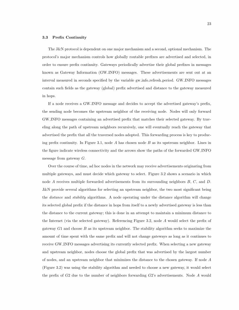
multiple gateways, and must decide which gateway to select. Figure 3.2 shows a scenario in which
node A receives multiple forwarded advertisements from its surrounding neighbors B, C, and D.
J&N provide several algorithms for selecting an upstream neighbor, the two most significant being
the distance and stability algorithms. A node operating under the distance algorithm will change
its selected global prefix if the distance in hops from itself to a newly advertised gateway is less than
the distance to the current gateway; this is done in an attempt to maintain a minimum distance to
the Internet (via the selected gateway). Referencing Figure 3.2, node A would select the prefix of
gateway G1 and choose B as its upstream neighbor. The stability algorithm seeks to maximize the
amount of time spent with the same prefix and will not change gateways as long as it continues to
receive GW INFO messages advertising its currently selected prefix. When selecting a new gateway
and upstream neighbor, nodes choose the global prefix that was advertised by the largest number
of nodes, and an upstream neighbor that minimizes the distance to the chosen gateway. If node A
(Figure 3.2) was using the stability algorithm and needed to choose a new gateway, it would select
the prefix of G2 due to the number of neighbors forwarding G2’s advertisements. Node A would
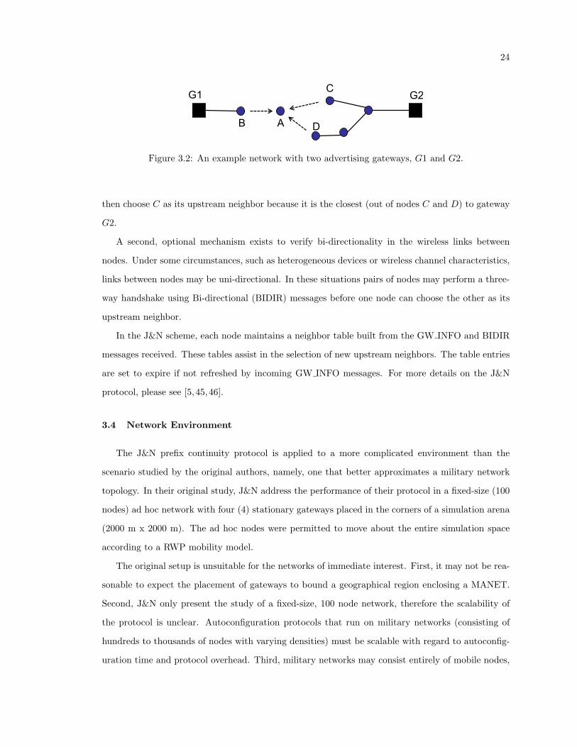
24
G1
A
G2
B
C
D
Figure 3.2: An example network with two advertising gateways, G1 and G2.
then choose C as its upstream neighbor because it is the closest (out of nodes C and D) to gateway
G2.
A second, optional mechanism exists to verify bi-directionality in the wireless links between
nodes. Under some circumstances, such as heterogeneous devices or wireless channel characteristics,
links between nodes may be uni-directional. In these situations pairs of nodes may perform a three-
way handshake using Bi-directional (BIDIR) messages before one node can choose the other as its
upstream neighbor.
In the J&N scheme, each node maintains a neighbor table built from the GW INFO and BIDIR
messages received. These tables assist in the selection of new upstream neighbors. The table entries
are set to expire if not refreshed by incoming GW INFO messages. For more details on the J&N
protocol, please see [5, 45,46].
3.4 Network Environment
The J&N prefix continuity protocol is applied to a more complicated environment than the
scenario studied by the original authors, namely, one that better approximates a military network
topology. In their original study, J&N address the performance of their protocol in a fixed-size (100
nodes) ad hoc network with four (4) stationary gateways placed in the corners of a simulation arena
(2000 m x 2000 m). The ad hoc nodes were permitted to move about the entire simulation space
according to a RWP mobility model.
The original setup is unsuitable for the networks of immediate interest. First, it may not be rea-
sonable to expect the placement of gateways to bound a geographical region enclosing a MANET.
Second, J&N only present the study of a fixed-size, 100 node network, therefore the scalability of
the protocol is unclear. Autoconfiguration protocols that run on military networks (consisting of
hundreds to thousands of nodes with varying densities) must be scalable with regard to autoconfig-
uration time and protocol overhead. Third, military networks may consist entirely of mobile nodes,
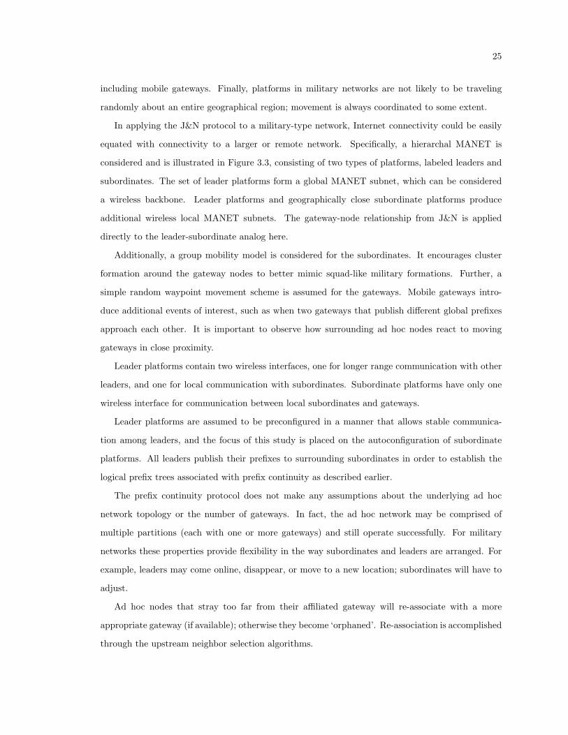
25
including mobile gateways. Finally, platforms in military networks are not likely to be traveling
randomly about an entire geographical region; movement is always coordinated to some extent.
In applying the J&N protocol to a military-type network, Internet connectivity could be easily
equated with connectivity to a larger or remote network. Specifically, a hierarchal MANET is
considered and is illustrated in Figure 3.3, consisting of two types of platforms, labeled leaders and
subordinates. The set of leader platforms form a global MANET subnet, which can be considered
a wireless backbone. Leader platforms and geographically close subordinate platforms produce
additional wireless local MANET subnets. The gateway-node relationship from J&N is applied
directly to the leader-subordinate analog here.
Additionally, a group mobility model is considered for the subordinates. It encourages cluster
formation around the gateway nodes to better mimic squad-like military formations. Further, a
simple random waypoint movement scheme is assumed for the gateways. Mobile gateways intro-
duce additional events of interest, such as when two gateways that publish different global prefixes
approach each other. It is important to observe how surrounding ad hoc nodes react to moving
gateways in close proximity.
Leader platforms contain two wireless interfaces, one for longer range communication with other
leaders, and one for local communication with subordinates. Subordinate platforms have only one
wireless interface for communication between local subordinates and gateways.
Leader platforms are assumed to be preconfigured in a manner that allows stable communica-
tion among leaders, and the focus of this study is placed on the autoconfiguration of subordinate
platforms. All leaders publish their prefixes to surrounding subordinates in order to establish the
logical prefix trees associated with prefix continuity as described earlier.
The prefix continuity protocol does not make any assumptions about the underlying ad hoc
network topology or the number of gateways. In fact, the ad hoc network may be comprised of
multiple partitions (each with one or more gateways) and still operate successfully. For military
networks these properties provide flexibility in the way subordinates and leaders are arranged. For
example, leaders may come online, disappear, or move to a new location; subordinates will have to
adjust.
Ad hoc nodes that stray too far from their affiliated gateway will re-associate with a more
appropriate gateway (if available); otherwise they become ‘orphaned’. Re-association is accomplished
through the upstream neighbor selection algorithms.
26
Local
Subnets
Global Subnet
Figure 3.3: The logical network topology under consideration. Leaders, denoted by squares, formthe backbone and serve as attachment points for the subordinates, represented as dots.
3.5 General Simulation Details
This section details the general scenario representation in OPNET Modeler version 12.0 [9].
Parameter values specific to a particular scenario, as well any exceptions to the general model setup
described are detailed later. Where possible, simulation parameters were set to values equal to those
used in the J&N study [5].
The simulation arena was a flat 2000 m by 2000 m square. Nah is used to designate the total
number of ad hoc nodes in the simulation arena, while Ngw represents the number of gateways.
Gateway and ad hoc nodes were built from the standard OPNET ‘manet station adv’ node model.
Since the wireless backbone formed by all leaders was not the focus of this particular study (and
therefore not actively simulated), gateways and ad hoc nodes each had only one Institute of Electrical
and Electronics Engineers (IEEE) 802.11 interface.
The default wireless propagation model in OPNET used the Friis transmission equation (2.1) as
shown in Section 2.3.3. The equation parameters were set such that a transmission had a maximum
range of 250 m under interference-free conditions. The transmitter and receiver antenna gains were
assumed to be isotropic and were both set to 0 dB. The pathloss exponent was set to 2 to reflect
free-space propagation, and the default OPNET noise figure of No = 8.80 × 10⁻¹⁴ W was used. A
transmission power of 0.2 mW and receiver sensitivity of −95 dBm was used to force the 250 m
distance limit on transmissions - if the received signal power was less than the receiver sensitivity,
the transmission was immediately considered unsuccessful. Transmissions were also subjected to

27
Signal to Interference and Noise Ratio (SINR) calculations using equations (2.2) and (2.7). Finally,
as discussed in Section 2.5, OPNET maps the SINR to a Bit Error Rate (BER) depending on the
modulation scheme in use by IEEE 802.11, and is configured to fail a transmission if any bit errors
are detected.
Application traffic was not modeled in the network. A ‘warm-up’ time of 3000 seconds was applied
to the mobility models so that the spatial distribution of nodes approached steady-state [24], after
which the J&N protocol was started and statistics began to be recorded.
3.5.1 Prefix Continuity Model
A model of the J&N prefix continuity protocol was constructed in OPNET based on [5,45,46]. It
was implemented as a stand-alone process model (i.e., not integrated with a specific routing protocol)
and interfaced with the User Datagram Protocol (UDP) transport layer protocol. BIDIR messages
were disabled, as all nodes used the same transmission power. Both the stability and distance
algorithms for upstream neighbor selection were studied. Prefix continuity protocol parameters,
which controlled timers and neighbor table entry timeout values, were set in accordance with [45].
3.5.2 Mobility Models
Mobile gateways were permitted to move about the entire simulation space according to a RWP
model [23] with a constant speed of 2.5 m/s and a pause time of 25 seconds.
Ad hoc nodes were assigned a group mobility model that consisted of a restricted RWP model.
At the beginning of the simulation, each node chose a random gateway uniformly from the set of all
gateways. The restricted RWP selection algorithm would choose waypoints within a specified region
of the chosen gateway. The destination selection was controlled by the parameter xy var, which
specified the maximum coordinate deviation in meters in both the horizontal and vertical directions
from the chosen leader. Ad hoc nodes moved at a constant speed of 5 m/s and had a pause time of
10 seconds. See Figure 3.4 for a visualization of this setup.
Under this mobility model, orphaned nodes may be caused if xy var is too large, permitting
the ad hoc nodes to stray too far away from available upstream neighbors, or if Nah is too small,
limiting the number of potential upstream neighbors.
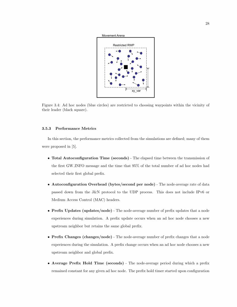
28
xy_var
Movement Arena
Restricted RWP
Figure 3.4: Ad hoc nodes (blue circles) are restricted to choosing waypoints within the vicinity oftheir leader (black square).
3.5.3 Performance Metrics
In this section, the performance metrics collected from the simulations are defined; many of them
were proposed in [5].
• Total Autoconfiguration Time (seconds) - The elapsed time between the transmission of
the first GW INFO message and the time that 95% of the total number of ad hoc nodes had
selected their first global prefix.
• Autoconfiguration Overhead (bytes/second per node) - The node-average rate of data
passed down from the J&N protocol to the UDP process. This does not include IPv6 or
Medium Access Control (MAC) headers.
• Prefix Updates (updates/node) - The node-average number of prefix updates that a node
experiences during simulation. A prefix update occurs when an ad hoc node chooses a new
upstream neighbor but retains the same global prefix.
• Prefix Changes (changes/node) - The node-average number of prefix changes that a node
experiences during the simulation. A prefix change occurs when an ad hoc node chooses a new
upstream neighbor and global prefix.
• Average Prefix Hold Time (seconds) - The node-average period during which a prefix
remained constant for any given ad hoc node. The prefix hold timer started upon configuration
29
of a new prefix and stopped for only the following events: a prefix change occurred, or the
upstream neighbor entry timed out.
• Percentage of Time Without a Prefix (%) - The node-average percentage of time a node
spent without a prefix, starting from the transmission of the first GW INFO message until the
end of the simulation.
3.6 Simulation Scenarios
In this section, we describe a validation scenario as well as three new scenarios (shown in Figure
3.5) used to capture the performance of the prefix continuity protocol. The primary goals of these
new scenarios are to quantify the following trends: (1) the performance of the protocol as the ratio
of the number of ad hoc nodes to gateways changes; (2) the scaling of the protocol’s overhead and
initial autoconfiguration time versus network size; and (3) the protocol’s performance under a group
mobility regime with various cluster densities. Each scenario combination was run ten (10) times.
All data presented is averaged over the 10 runs.
3.6.1 Validation Scenario
We first validated our OPNET implementation with J&N’s data. To this end, the scenario
presented in their original paper [5] was replicated. J&N’s simulation arena consisted of a flat 2000
m by 2000 m area with a stationary gateway placed in each corner, 250 m away from each edge.
Each gateway advertised a unique prefix. One hundred nodes moved about the simulation space
according to random waypoint with speeds chosen uniformly from the range [0.5, 1.5] m/s and pause
times of 150 seconds. Simulations of this scenario were run for both upstream neighbor algorithms.
Each simulation run lasted 65 simulated minutes (50 minutes for mobility model ‘warm-up’ time
plus 15 minutes of protocol operation).
3.6.2 Scenario I: Single, Stationary Gateway
The first new scenario examined the effect of scaling the number of ad hoc nodes, Nah, for
a single stationary gateway (Ngw = 1) located at the center of the (square) simulation arena.
This scenario helps shed light on how the prefix continuity protocol behaves in the presence of
larger and more dense networks. Nah was varied from 25 to 400 nodes. For each ad hoc network
size, the group mobility parameter xy var was varied from 250 to 1000 meters so that the ad hoc

30
2000m
2*(xy_var)
2*(xy_var)
1 2 3
2000m
Figure 3.5: Scenarios I-III are shown from left to right.
nodes movement became less dependent on the chosen leader. Only the distance upstream neighbor
selection algorithm was studied under this scenario (the stability algorithm simplifies to the distance
algorithm in the presence of only one advertised prefix). Each simulation run lasted 65 simulated
minutes (using the same warm-up/operation division as in the validation section).
3.6.3 Scenario II: Single, Mobile Gateway
The second scenario studied the effect of gateway mobility for a single gateway (Ngw = 1). Nah
and xy var were varied as in Scenario I. The gateway node was configured to move around the
simulation arena under the unrestricted random waypoint model described in Section 3.5. Again,
only the distance algorithm was simulated in this scenario. Each simulation run lasted 75 simulated
minutes (adding 10 extra minutes to the protocol operation).
3.6.4 Scenario III: Multiple, Mobile Gateways
Finally, multiple gateways were permitted to move without restriction in the simulation space
for the third scenario. The number of gateways, Ngw, was varied from 1 to 4. Each gateway was set
to advertise a unique global prefix. For each selection of Ngw, several values for the ad hoc network
size, Nah, were tested while xy var was fixed at 500 m. Each simulation run lasted 75 minutes, as
in the previous scenario.
3.7 Simulation Results
In general, the OPNET implementation of the J&N protocol performed as expected and was
comparable to the data presented in [5], including autoconfiguration time, prefix updates, prefix
31
changes, and prefix hold time. For data relating to the autoconfiguration time (‘convergence’ in [5]),
prefix changes per node, and prefix updates per node, similar trends were found for both upstream
neighbor selection algorithms. However, there was a difference in the reported average prefix hold
time. Our OPNET simulations reported an average prefix hold time on the order of ten (10) seconds
for both upstream neighbor algorithms, while J&N reported average prefix hold times on the order
of one hundred (100) seconds for the stability algorithm.
After discussion with the original authors, it was found that our OPNET validation scenario
did not include stationary relay nodes that were used to increase the effective transmission range of
the gateways in [47]. These nodes served to counteract the RWP steady-state distribution of node
positions, located around the center of the simulation arena. The lack of relay nodes made it easier for
the gateways to become disconnected from the MANET, potentially driving the OPNET-measured
prefix hold times lower.
Other potential sources for these differences include inherent differences in the simulators [15]
(J&N used the network simulator, ns-2, in [5]) and differences in the interpretation of how the metric
should be measured.
3.7.1 Scenario I: Single, Stationary Gateway
Figures 3.6 and 3.7 address the scaling of the total autoconfiguration time and the prefix conti-
nuity protocol overhead, as the number of nodes in the ad hoc network increases around a single,
stationary gateway for various cluster sizes (controlled by xy var).
Figure 3.6 shows the total autoconfiguration time (in seconds) versus the number of ad hoc
nodes in the network, while the cluster size variable, xy var, serves as a parameter. The measured
autoconfiguration times show a strong dependence on the density of the cluster around the gateway.
The density of the network can be increased in two ways: by adding more ad hoc nodes (Nah) to
the network, or by making the cluster area smaller, via xy var. In both cases, the autoconfiguration
times decrease for more dense networks. This is largely attributed to nodes already being within
range of a potential upstream neighbor in order to autoconfigure for the first time. In less dense
networks, more time is spent waiting for nodes to move within range of potential upstream neighbors,
and a larger total autoconfiguration time is recorded.
Figure 3.7 shows the overhead per node (in bytes/second) versus the number of nodes, Nah, in
the ad hoc network, while xy var serves as a parameter controlling the cluster area. Increasing the
density of the cluster around the gateway, either by increasing Nah or by decreasing xy var, tends to
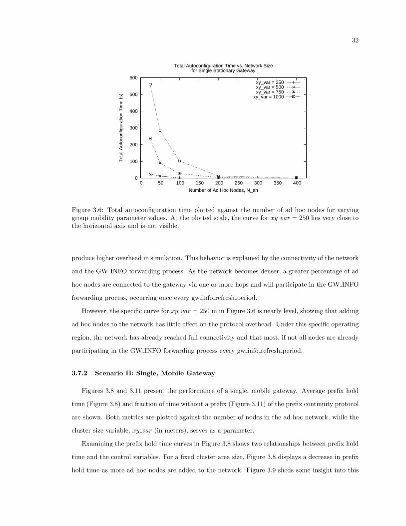
32
0
100
200
300
400
500
600
0 50 100 150 200 250 300 350 400
Tot
al A
utoc
onfig
urat
ion
Tim
e (s
)
Number of Ad Hoc Nodes, N_ah
Total Autoconfiguration Time vs. Network Sizefor Single Stationary Gateway
xy_var = 250xy_var = 500xy_var = 750
xy_var = 1000
Figure 3.6: Total autoconfiguration time plotted against the number of ad hoc nodes for varyinggroup mobility parameter values. At the plotted scale, the curve for xy var = 250 lies very close tothe horizontal axis and is not visible.
produce higher overhead in simulation. This behavior is explained by the connectivity of the network
and the GW INFO forwarding process. As the network becomes denser, a greater percentage of ad
hoc nodes are connected to the gateway via one or more hops and will participate in the GW INFO
forwarding process, occurring once every gw info refresh period.
However, the specific curve for xy var = 250 m in Figure 3.6 is nearly level, showing that adding
ad hoc nodes to the network has little effect on the protocol overhead. Under this specific operating
region, the network has already reached full connectivity and that most, if not all nodes are already
participating in the GW INFO forwarding process every gw info refresh period.
3.7.2 Scenario II: Single, Mobile Gateway
Figures 3.8 and 3.11 present the performance of a single, mobile gateway. Average prefix hold
time (Figure 3.8) and fraction of time without a prefix (Figure 3.11) of the prefix continuity protocol
are shown. Both metrics are plotted against the number of nodes in the ad hoc network, while the
cluster size variable, xy var (in meters), serves as a parameter.
Examining the prefix hold time curves in Figure 3.8 shows two relationships between prefix hold
time and the control variables. For a fixed cluster area size, Figure 3.8 displays a decrease in prefix
hold time as more ad hoc nodes are added to the network. Figure 3.9 sheds some insight into this
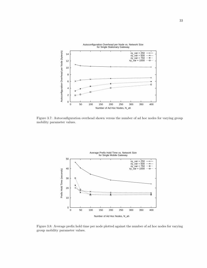
33
0
2
4
6
8
10
12
14
0 50 100 150 200 250 300 350 400
Aut
ocon
figur
atio
n O
verh
ead
per
Nod
e (b
ytes
/s)
Number of Ad Hoc Nodes, N_ah
Autoconfiguration Overhead per Node vs. Network Sizefor Single Stationary Gateway
xy_var = 250xy_var = 500xy_var = 750
xy_var = 1000
Figure 3.7: Autoconfiguration overhead shown versus the number of ad hoc nodes for varying groupmobility parameter values.
0
10
20
30
40
50
0 50 100 150 200 250 300 350 400
Pre
fix H
old
Tim
e (s
econ
ds)
Number of Ad Hoc Nodes, N_ah
Average Prefix Hold Time vs. Network Sizefor Single Mobile Gateway
xy_var = 250xy_var = 500xy_var = 750
xy_var = 1000
Figure 3.8: Average prefix hold time per node plotted against the number of ad hoc nodes for varyinggroup mobility parameter values.
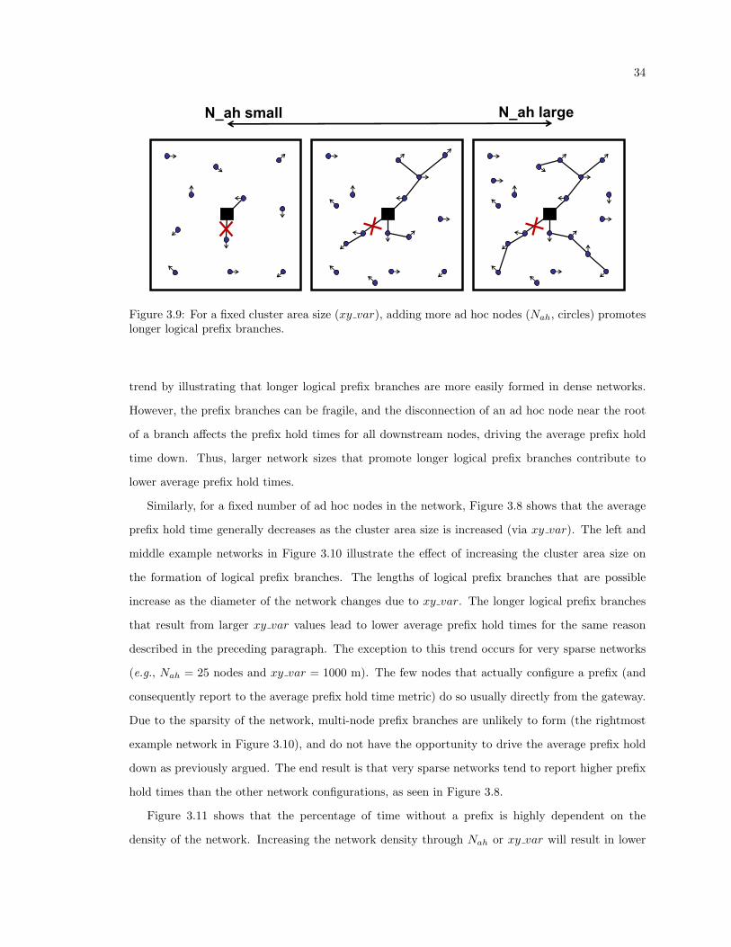
34
N_ah small N_ah large
Figure 3.9: For a fixed cluster area size (xy var), adding more ad hoc nodes (Nah, circles) promoteslonger logical prefix branches.
trend by illustrating that longer logical prefix branches are more easily formed in dense networks.
However, the prefix branches can be fragile, and the disconnection of an ad hoc node near the root
of a branch affects the prefix hold times for all downstream nodes, driving the average prefix hold
time down. Thus, larger network sizes that promote longer logical prefix branches contribute to
lower average prefix hold times.
Similarly, for a fixed number of ad hoc nodes in the network, Figure 3.8 shows that the average
prefix hold time generally decreases as the cluster area size is increased (via xy var). The left and
middle example networks in Figure 3.10 illustrate the effect of increasing the cluster area size on
the formation of logical prefix branches. The lengths of logical prefix branches that are possible
increase as the diameter of the network changes due to xy var. The longer logical prefix branches
that result from larger xy var values lead to lower average prefix hold times for the same reason
described in the preceding paragraph. The exception to this trend occurs for very sparse networks
(e.g., Nah = 25 nodes and xy var = 1000 m). The few nodes that actually configure a prefix (and
consequently report to the average prefix hold time metric) do so usually directly from the gateway.
Due to the sparsity of the network, multi-node prefix branches are unlikely to form (the rightmost
example network in Figure 3.10), and do not have the opportunity to drive the average prefix hold
down as previously argued. The end result is that very sparse networks tend to report higher prefix
hold times than the other network configurations, as seen in Figure 3.8.
Figure 3.11 shows that the percentage of time without a prefix is highly dependent on the
density of the network. Increasing the network density through Nah or xy var will result in lower
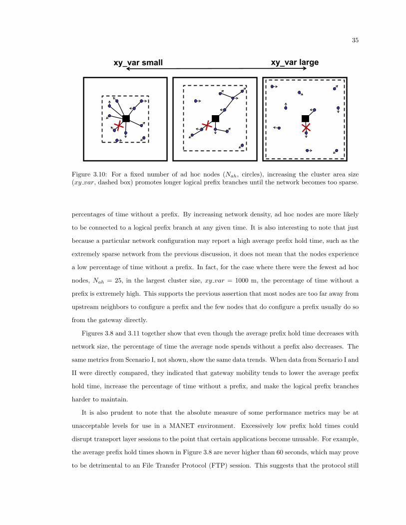
35
xy_var small xy_var large
Figure 3.10: For a fixed number of ad hoc nodes (Nah, circles), increasing the cluster area size(xy var, dashed box) promotes longer logical prefix branches until the network becomes too sparse.
percentages of time without a prefix. By increasing network density, ad hoc nodes are more likely
to be connected to a logical prefix branch at any given time. It is also interesting to note that just
because a particular network configuration may report a high average prefix hold time, such as the
extremely sparse network from the previous discussion, it does not mean that the nodes experience
a low percentage of time without a prefix. In fact, for the case where there were the fewest ad hoc
nodes, Nah = 25, in the largest cluster size, xy var = 1000 m, the percentage of time without a
prefix is extremely high. This supports the previous assertion that most nodes are too far away from
upstream neighbors to configure a prefix and the few nodes that do configure a prefix usually do so
from the gateway directly.
Figures 3.8 and 3.11 together show that even though the average prefix hold time decreases with
network size, the percentage of time the average node spends without a prefix also decreases. The
same metrics from Scenario I, not shown, show the same data trends. When data from Scenario I and
II were directly compared, they indicated that gateway mobility tends to lower the average prefix
hold time, increase the percentage of time without a prefix, and make the logical prefix branches
harder to maintain.
It is also prudent to note that the absolute measure of some performance metrics may be at
unacceptable levels for use in a MANET environment. Excessively low prefix hold times could
disrupt transport layer sessions to the point that certain applications become unusable. For example,
the average prefix hold times shown in Figure 3.8 are never higher than 60 seconds, which may prove
to be detrimental to an File Transfer Protocol (FTP) session. This suggests that the protocol still
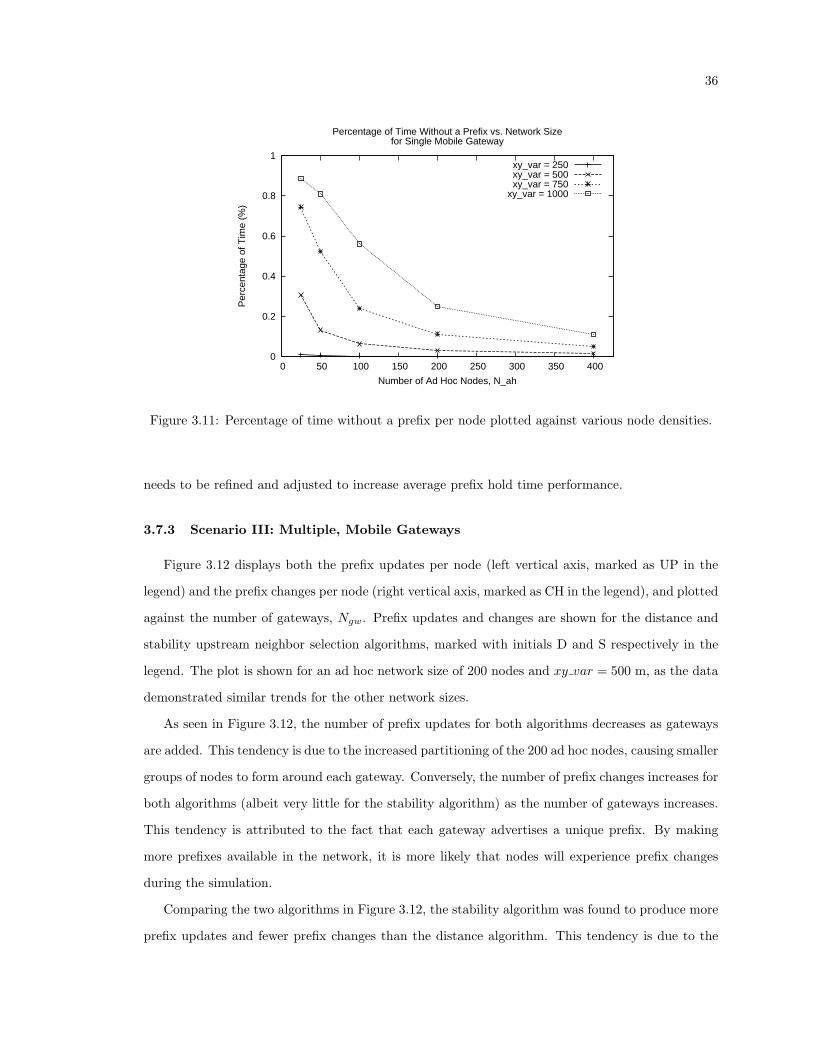
36
0
0.2
0.4
0.6
0.8
1
0 50 100 150 200 250 300 350 400
Per
cent
age
of T
ime
(%)
Number of Ad Hoc Nodes, N_ah
Percentage of Time Without a Prefix vs. Network Sizefor Single Mobile Gateway
xy_var = 250xy_var = 500xy_var = 750
xy_var = 1000
Figure 3.11: Percentage of time without a prefix per node plotted against various node densities.
needs to be refined and adjusted to increase average prefix hold time performance.
3.7.3 Scenario III: Multiple, Mobile Gateways
Figure 3.12 displays both the prefix updates per node (left vertical axis, marked as UP in the
legend) and the prefix changes per node (right vertical axis, marked as CH in the legend), and plotted
against the number of gateways, Ngw. Prefix updates and changes are shown for the distance and
stability upstream neighbor selection algorithms, marked with initials D and S respectively in the
legend. The plot is shown for an ad hoc network size of 200 nodes and xy var = 500 m, as the data
demonstrated similar trends for the other network sizes.
As seen in Figure 3.12, the number of prefix updates for both algorithms decreases as gateways
are added. This tendency is due to the increased partitioning of the 200 ad hoc nodes, causing smaller
groups of nodes to form around each gateway. Conversely, the number of prefix changes increases for
both algorithms (albeit very little for the stability algorithm) as the number of gateways increases.
This tendency is attributed to the fact that each gateway advertises a unique prefix. By making
more prefixes available in the network, it is more likely that nodes will experience prefix changes
during the simulation.
Comparing the two algorithms in Figure 3.12, the stability algorithm was found to produce more
prefix updates and fewer prefix changes than the distance algorithm. This tendency is due to the
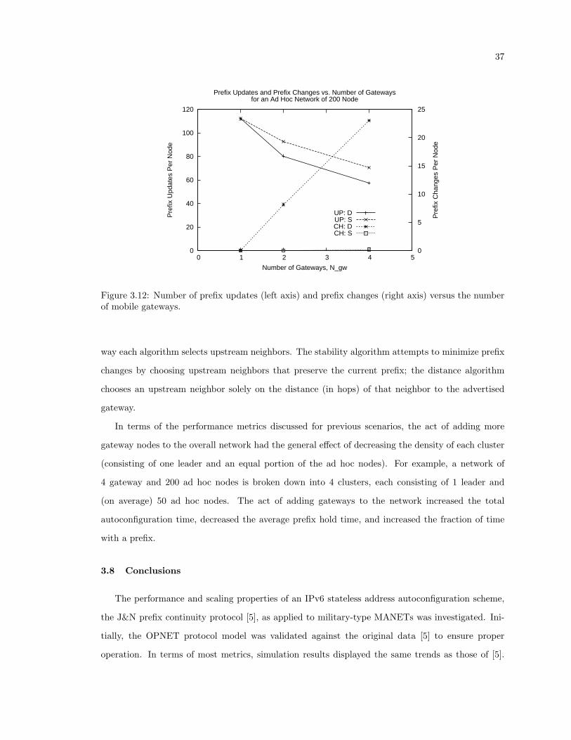
37
0
20
40
60
80
100
120
0 1 2 3 4 5 0
5
10
15
20
25
Pre
fix U
pdat
es P
er N
ode
Pre
fix C
hang
es P
er N
ode
Number of Gateways, N_gw
Prefix Updates and Prefix Changes vs. Number of Gatewaysfor an Ad Hoc Network of 200 Node
UP: DUP: SCH: DCH: S
Figure 3.12: Number of prefix updates (left axis) and prefix changes (right axis) versus the numberof mobile gateways.
way each algorithm selects upstream neighbors. The stability algorithm attempts to minimize prefix
changes by choosing upstream neighbors that preserve the current prefix; the distance algorithm
chooses an upstream neighbor solely on the distance (in hops) of that neighbor to the advertised
gateway.
In terms of the performance metrics discussed for previous scenarios, the act of adding more
gateway nodes to the overall network had the general effect of decreasing the density of each cluster
(consisting of one leader and an equal portion of the ad hoc nodes). For example, a network of
4 gateway and 200 ad hoc nodes is broken down into 4 clusters, each consisting of 1 leader and
(on average) 50 ad hoc nodes. The act of adding gateways to the network increased the total
autoconfiguration time, decreased the average prefix hold time, and increased the fraction of time
with a prefix.
3.8 Conclusions
The performance and scaling properties of an IPv6 stateless address autoconfiguration scheme,
the J&N prefix continuity protocol [5], as applied to military-type MANETs was investigated. Ini-
tially, the OPNET protocol model was validated against the original data [5] to ensure proper
operation. In terms of most metrics, simulation results displayed the same trends as those of [5].

38
However, there were noted differences in prefix hold times with several potential sources for such
differences. Next, the scalability of a single, stationary gateway was examined. Subsequently, focus
was placed on protocol performance under a single, mobile gateway. Finally, general performance
characteristics were gathered when multiple mobile gateways were present in the network.
In the single stationary gateway scenario (Scenario I), large network densities achieved rapid
autoconfiguration times. Although the autoconfiguration overhead was higher for dense clusters,
the overhead in general was very low when BIDIR messages are disabled. Hence the protocol shows
potential for military networks where bandwidth availability is a concern and routing protocols can
validate bi-directionality in links.
By permitting gateways to move in a simple random waypoint scheme in Scenario II, the pro-
tocol’s performance was impacted. Gateway mobility increased the percentage of time without a
prefix and decreased the prefix hold time. It was found that adding more ad hoc nodes to the
network tended to decrease the percentage of time without a prefix as well as the prefix hold time,
suggesting a tradeoff to be investigated further. The low prefix hold time measurements in general
suggested that ad hoc nodes may experience difficulties in maintaining higher layer sessions. The
J&N protocol may need be revised further to improve performance in this area.
Allowing multiple clusters to move around freely in the arena enabled the observation of how
the two neighbor selection algorithms handled gateway mobility. The stability algorithm resulted in
a multitude of prefix updates and very few prefix changes, as it was designed to maximize average
prefix hold time. The distance algorithm registered more prefix changes per node as a result of its
focus on minimizing distance (in hops) to the chosen gateway. Additionally, it was observed that
adding more gateways effectively lowered the network density for each cluster, yielding changes in
performance that conformed to results from the previous scenarios.
3.9 Future Work
Future studies should address the feasibility of a hierarchical layering of the prefix continuity
protocol, such that mobile gateways would first autoconfigure their prefixes from one or more status-
elevated gateways. Autoconfiguration of the ad hoc nodes underneath would then take place after
a gateway completed its own autoconfiguration.
Allowing multiple gateways in the same mobile group to advertise the same prefix is another
scenario of interest. This capability could provide faster autoconfiguration time while possibly also

39
increasing prefix stability.
Third, it is worthwhile to investigate the performance of the prefix continuity protocol in light of
the ‘parking lot’ problem. A network may specifically autoconfigure in a static topology, or ‘parked’
state, and mobilize afterward.
Attention should also be given to the notion of an optimal gateway-to-ad hoc node ratio. Such
a study should seek to find a threshold where the selected number of gateways balance metrics such
as percentage of time without a prefix and prefix hold time.
40
4. Simulation Cross-Validation of Emulation Testbed∗
4.1 Introduction
Accurate performance prediction and testing of communications devices and protocols before
deployment and standardization is a necessity. Implementation bugs and poor designs that are
passed on to consumers discourage adoption and success in the marketplace. Certain scenarios,
such as tactical military deployments and rescue operations, are far less forgiving when it comes
to operational errors of communications technology. Network simulation and emulation are two
common tools used during development to catch and fix such flaws in design and implementation.
These tools provide independent methods of validating the performance of new protocols, as well as
provide feedback on correct protocol implementation and configuration.
While simulation and emulation are in and of themselves very useful, each offers advantages that
cover shortcomings of the other. Discrete event simulations can offer extensive debugging and event
control capabilities as well as reproducible sequences of events. Emulation testbeds, which typically
run live implementations at the network layer and above on top of emulated links (substituted
medium access and physical layers), cannot so easily stop and step through time. Furthermore,
emulations are locked into a 1:1 ‘real-time’ run time, which is not the case for simulations. Depending
on the complexity of simulation models, faster than real-time results can be collected and analyzed,
which is important for long duration experiments. Additionally, scaling simulations to study large
networks is much more cost effective than using an emulation testbed. However, it has been argued
that emulation testbeds offer more realistic network behavior than simulations [3] due to the fact
that actual implementation code is run on network devices. Relying on simulation alone may in
fact hide design flaws in the protocols due to code or hardware differences, that would otherwise
be revealed when emulating the same network [1]. Instead, using both methods together to study
network protocols builds confidence that the protocols in question are configured and operating
correctly.
Recent work in the Internet Engineering Task Force (IETF) has produced three proposed exten-
sions to the Open Shortest Path First version 3 (OSPFv3) routing protocol that are better suited for
∗This work was done while J. Wildman was an intern at MIT Lincoln Lab over the summer of 2007. Constructiveand helpful guidance was provided by both supervisor, Dr. Siamak Dastangoo, and fellow intern, Dr. Glenn Carl.Duties included development and management of simulations in support of Dr. Carl’s emulation testbed experiments.
41
the lower data rate and dynamic topology of Mobile Ad hoc Networks (MANETs) [48–50]. These
extensions are prime candidates for comparative studies using simulation and emulation methods as
they are new and still in development. This chapter details an effort to study and compare different
operating modes of one of the OSPFv3 extensions, called MANET Designated Router (MDR), in
both a simulation and emulation environment. The measured Open Shortest Path First (OSPF)
overhead from both environments was used as a benchmark to construct equivalent MANET repre-
sentations and protocol configuration, made particularly challenging due to the wired nature of the
emulation testbed. During the process of results matching, limitations of the simulated implemen-
tation of OSPF were revealed.
Within this chapter, particular attention is given to the simulation environment, as extensive
details on the setup and experimentation process of the emulation testbed setup are provided in [7].
Section 4.2 provides background on the OSPFv3 protocol and its proposed MDR extension. Sec-
tion 4.3 introduces the different environments and OSPF implementations (OPNET simulation and
emulation testbed) being cross-validated. Section 4.4 details the efforts involved in the construction
of equivalent simulation and emulation environments. Section 4.5 compares the simulation perfor-
mance results to the emulated testbed. Sections 4.6 and 4.7 present the conclusions and provide
future directions of work, respectively.
4.2 Background on Open Shortest Path First (OSPF)
OSPF is a widely used link-state driven routing protocol. Development and standardization of
the protocol has spanned roughly two decades and has generated three versions, starting with the
formation of the IETF OSPF working group in 1987 and continuing with OSPFv3 and its numerous
extensions as of the time of this writing.
OSPFv1, which quickly evolved to OSPFv2, was designed for Internet Protocol (IP)v4 networks.
The last Request for Comments (RFC) released for OSPFv2 was RFC 2328 in 1998 [51]. OSPFv2
was then extended in RFC 2740 to support Internet Protocol version 6 (IPv6) in 1999 as OSPFv3
(or OSPF for IPv6) [52]. Numerous small revisions to the initial RFC have been compiled in an
updated version of OSPFv3, RFC 5340 [53].
There have been numerous efforts to develop extensions to OSPF(v2 and v3) that are better
suited to wireless environments. These include Radio-OSPF (R-OSPF), a proprietary extension
to OSPFv2 developed by BBN Technologies cited in [54], and Wireless OSPF, a proposal made by
42
Boeing Phantom Works that defines a new type of OSPFv2 interface to limit the number of adjacen-
cies formed between wireless nodes in an attempt to cut down on excessive protocol overhead [55].
Additionally, two competing ‘wireless’ extensions to OSPFv3, Cisco Systems-developed Overlapping
Relays (OR) [56] and the proposal MDR [57] by Richard Ogier, were thoroughly compared through
simulation in [58]. The latest revisions of the OR and MDR drafts are [48] and [49] respectively. A
third proposal, called the OSPF Multipoint Relay (MPR) extension [50], incorporates the concept
of multipoint relaying from the Optimized Link State Routing (OLSR) protocol into the OSPFv3
protocol framework.
The remaining part of this section provides a general overview of OSPFv3 routing protocol
operation. Since the simulation and emulation work described in later sections concerns only OSPFv3
and the MDR extension, discussion involving other wireless adaptations of OSPF is omitted. Major
literature references for OSPF, excluding RFCs and Internet Drafts, are [59–61].
4.2.1 Overview of OSPFv3
OSPFv3 is a proactive, link-state routing protocol. Routers actively maintain link-state informa-
tion between all routers in the network and store this information in a link-state database. Changes
to one router’s link-state database trigger the flooding of an update to the rest of the network along
existing links between routers.
Messages
In an OSPFv3 network, routers distribute and collect information to and from each other in
order to build routing tables. There are several types of messages that OSPFv3 routers exchange:
• Hello - Routers transmit periodic Hello messages in order to inform nearby routers of available
links. Routers that exchange Hello messages become neighbors.
• Database Description (DbDesc) - Once a pair of routers become neighbors, they exchange
lists of stored routing information (the routers’ databases) through DbDesc messages.
• Link State Request (LSReq) - While exchanging DbDesc messages, one of the routers may
discover that it does not have the same information as its neighbor. A router can request
particular information from its neighbors with LSReq messages.
• Link State Update (LSU) - As routers learn new information from or about neighbors,
they flood this information out over the network in the form of LSUs. LSUs are comprised of

43
one or more Link State Advertisements (LSAs), containing information on neighboring routers,
network address prefixes, protocol configuration values, etc. Several types of LSAs have been
defined for OSPFv3 including Router, Network, Inter-Area Prefix, Intra-Area Prefix, Intra-Area
Router, AS-External, and Link LSAs.
• Link State Acknowledgement (LSAck) - LSAck messages acknowledge the receipt of LSUs
and help ensure that flooded information reaches the entire network.
Neighbors
As routers discover each other and synchronize databases, each router will associate specific
neighbor states to the other connected routers to describe the relationship between them. A few of
the important states follow, using the example of two routers, A and B:
• Down - Router A is unable to communicate with router B. Router B is considered to be
unreachable, or Down, to router A.
• Two-Way - Hello messages have been exchanged between routers A and B, meaning bi-
directional communication is possible between them. Routers A and B are considered to be
Two-Way neighbors of each other. However, neither router participates in the flooding of an
LSU sent by the other router.
• Full - If routers A and B are Two-Way neighbors, they may synchronize databases with each
other, to become Full neighbors, or adjacent to one another. LSUs are flooded over adjacencies
(links connecting the router to a Full neighbor) only. The procedure to determine whether
or not Two-Way neighbors form adjacencies is controlled by the routers’ configured interface
type.
Interface/Network Types
The interfaces of an OSPFv3 router are assigned specific interface types during router config-
uration. An interface type controls the decision process for forming adjacencies with neighboring
routers, as well as the LSU flooding procedure. There are several interface types defined in OSPFv3,
which were designed with wired networks in mind. The notion of network type comes from the
fact that routers on a common link are configured with the same interface type. The relevant
interface/network types in OSPFv3 include:
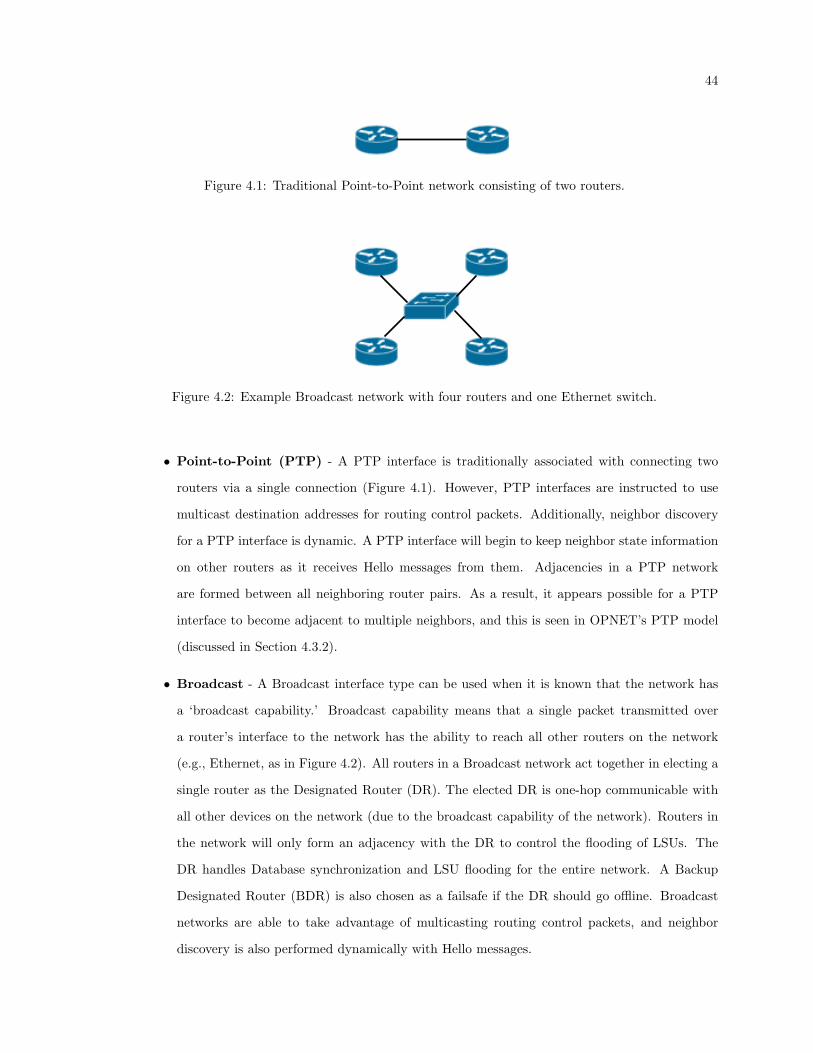
44
Figure 4.1: Traditional Point-to-Point network consisting of two routers.
Figure 4.2: Example Broadcast network with four routers and one Ethernet switch.
• Point-to-Point (PTP) - A PTP interface is traditionally associated with connecting two
routers via a single connection (Figure 4.1). However, PTP interfaces are instructed to use
multicast destination addresses for routing control packets. Additionally, neighbor discovery
for a PTP interface is dynamic. A PTP interface will begin to keep neighbor state information
on other routers as it receives Hello messages from them. Adjacencies in a PTP network
are formed between all neighboring router pairs. As a result, it appears possible for a PTP
interface to become adjacent to multiple neighbors, and this is seen in OPNET’s PTP model
(discussed in Section 4.3.2).
• Broadcast - A Broadcast interface type can be used when it is known that the network has
a ‘broadcast capability.’ Broadcast capability means that a single packet transmitted over
a router’s interface to the network has the ability to reach all other routers on the network
(e.g., Ethernet, as in Figure 4.2). All routers in a Broadcast network act together in electing a
single router as the Designated Router (DR). The elected DR is one-hop communicable with
all other devices on the network (due to the broadcast capability of the network). Routers in
the network will only form an adjacency with the DR to control the flooding of LSUs. The
DR handles Database synchronization and LSU flooding for the entire network. A Backup
Designated Router (BDR) is also chosen as a failsafe if the DR should go offline. Broadcast
networks are able to take advantage of multicasting routing control packets, and neighbor
discovery is also performed dynamically with Hello messages.
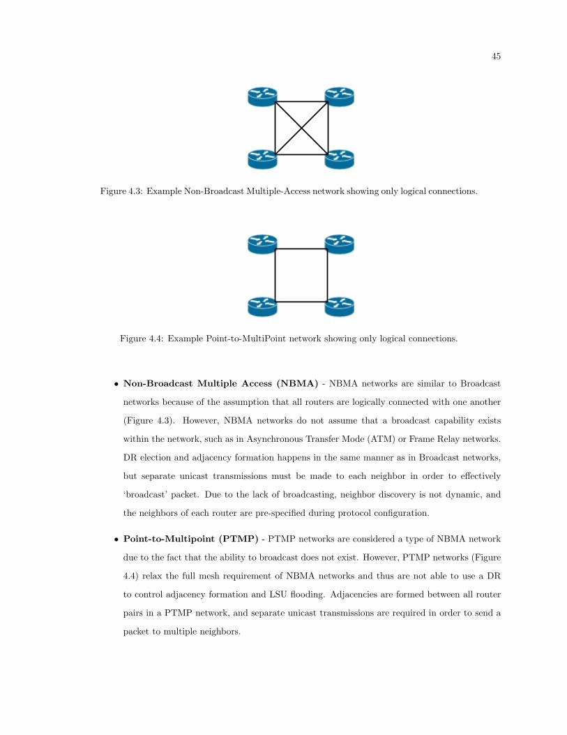
45
Figure 4.3: Example Non-Broadcast Multiple-Access network showing only logical connections.
Figure 4.4: Example Point-to-MultiPoint network showing only logical connections.
• Non-Broadcast Multiple Access (NBMA) - NBMA networks are similar to Broadcast
networks because of the assumption that all routers are logically connected with one another
(Figure 4.3). However, NBMA networks do not assume that a broadcast capability exists
within the network, such as in Asynchronous Transfer Mode (ATM) or Frame Relay networks.
DR election and adjacency formation happens in the same manner as in Broadcast networks,
but separate unicast transmissions must be made to each neighbor in order to effectively
‘broadcast’ packet. Due to the lack of broadcasting, neighbor discovery is not dynamic, and
the neighbors of each router are pre-specified during protocol configuration.
• Point-to-Multipoint (PTMP) - PTMP networks are considered a type of NBMA network
due to the fact that the ability to broadcast does not exist. However, PTMP networks (Figure
4.4) relax the full mesh requirement of NBMA networks and thus are not able to use a DR
to control adjacency formation and LSU flooding. Adjacencies are formed between all router
pairs in a PTMP network, and separate unicast transmissions are required in order to send a
packet to multiple neighbors.
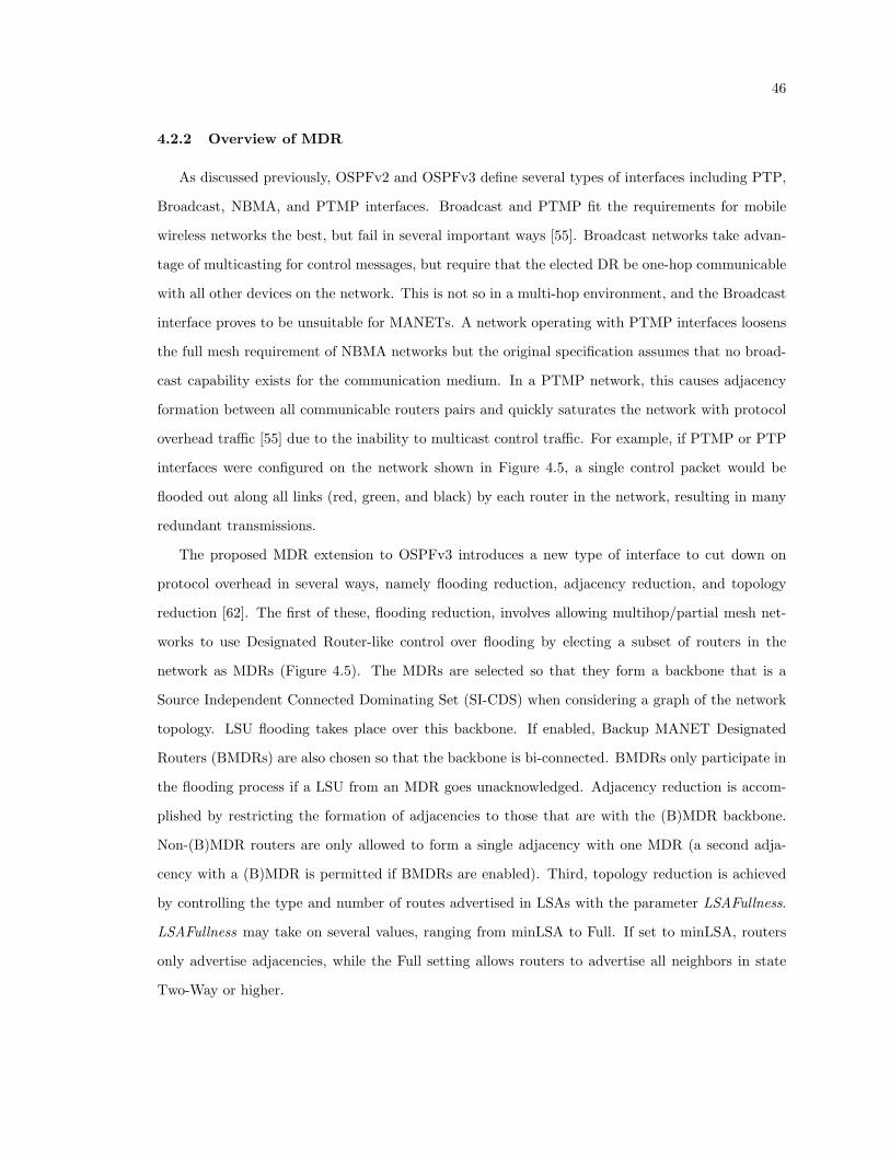
46
4.2.2 Overview of MDR
As discussed previously, OSPFv2 and OSPFv3 define several types of interfaces including PTP,
Broadcast, NBMA, and PTMP interfaces. Broadcast and PTMP fit the requirements for mobile
wireless networks the best, but fail in several important ways [55]. Broadcast networks take advan-
tage of multicasting for control messages, but require that the elected DR be one-hop communicable
with all other devices on the network. This is not so in a multi-hop environment, and the Broadcast
interface proves to be unsuitable for MANETs. A network operating with PTMP interfaces loosens
the full mesh requirement of NBMA networks but the original specification assumes that no broad-
cast capability exists for the communication medium. In a PTMP network, this causes adjacency
formation between all communicable routers pairs and quickly saturates the network with protocol
overhead traffic [55] due to the inability to multicast control traffic. For example, if PTMP or PTP
interfaces were configured on the network shown in Figure 4.5, a single control packet would be
flooded out along all links (red, green, and black) by each router in the network, resulting in many
redundant transmissions.
The proposed MDR extension to OSPFv3 introduces a new type of interface to cut down on
protocol overhead in several ways, namely flooding reduction, adjacency reduction, and topology
reduction [62]. The first of these, flooding reduction, involves allowing multihop/partial mesh net-
works to use Designated Router-like control over flooding by electing a subset of routers in the
network as MDRs (Figure 4.5). The MDRs are selected so that they form a backbone that is a
Source Independent Connected Dominating Set (SI-CDS) when considering a graph of the network
topology. LSU flooding takes place over this backbone. If enabled, Backup MANET Designated
Routers (BMDRs) are also chosen so that the backbone is bi-connected. BMDRs only participate in
the flooding process if a LSU from an MDR goes unacknowledged. Adjacency reduction is accom-
plished by restricting the formation of adjacencies to those that are with the (B)MDR backbone.
Non-(B)MDR routers are only allowed to form a single adjacency with one MDR (a second adja-
cency with a (B)MDR is permitted if BMDRs are enabled). Third, topology reduction is achieved
by controlling the type and number of routes advertised in LSAs with the parameter LSAFullness.
LSAFullness may take on several values, ranging from minLSA to Full. If set to minLSA, routers
only advertise adjacencies, while the Full setting allows routers to advertise all neighbors in state
Two-Way or higher.
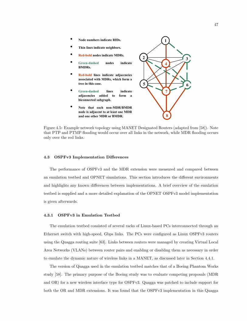
47
1
7
8
4
3
6 5
2
• Node numbers indicate RIDs.
• Thin lines indicate neighbors.
• Red-bold nodes indicate MDRs.
• Green-dashed nodes indicate
BMDRs.
• Red-bold lines indicate adjacencies
associated with MDRs, which form a
tree in this case.
• Green-dashed lines indicate
adjacencies added to form a
biconnected subgraph.
• Note that each non-MDR/BMDR
node is adjacent to at least one MDR
and one other MDR or BMDR.
Figure 4.5: Example network topology using MANET Designated Routers (adapted from [58]). Notethat PTP and PTMP flooding would occur over all links in the network, while MDR flooding occursonly over the red links.
4.3 OSPFv3 Implementation Differences
The performance of OSPFv3 and the MDR extension were measured and compared between
an emulation testbed and OPNET simulations. This section introduces the different environments
and highlights any known differences between implementations. A brief overview of the emulation
testbed is supplied and a more detailed explanation of the OPNET OSPFv3 model implementation
is given afterwards.
4.3.1 OSPFv3 in Emulation Testbed
The emulation testbed consisted of several racks of Linux-based PCs interconnected through an
Ethernet switch with high-speed, Gbps links. The PCs were configured as Linux OSPFv3 routers
using the Quagga routing suite [63]. Links between routers were managed by creating Virtual Local
Area Networks (VLANs) between router pairs and enabling or disabling them as necessary in order
to emulate the dynamic nature of wireless links in a MANET, as discussed later in Section 4.4.1.
The version of Quagga used in the emulation testbed matches that of a Boeing Phantom Works
study [58]. The primary purpose of the Boeing study was to evaluate competing proposals (MDR
and OR) for a new wireless interface type for OSPFv3. Quagga was patched to include support for
both the OR and MDR extensions. It was found that the OSPFv3 implementation in this Quagga
48
package (including the Boeing patches) included multicast support for PTMP interfaces. The MDR
extension implementation was cited by [58] to be generally consistent with the 4th version of the
Internet Draft [57]. More information can be found in [55,58,62]. For a thorough explanation of the
emulation testbed setup and management, refer to [7].
4.3.2 OSPFv3 in OPNET
Simulations were performed using OPNET Modeler 12.0 PL5 on a Linux platform running the
Redhat Enterprise Linux WS release 4 (Nahant Update 5) operating system. For reasons explained
later in this section, a custom patch was needed for OPNET’s OSPFv3 PTP interface. There
were many resources that were used to become more familiar with the OPNET implementation
of OSPFv2, OSPFv3, and the MDR extension, including OPNET Documentation, FAQ’s, and
[51,52,59–61,64]
Interface/Network Types
The standard interface types in OPNET generally operate in the manner described in Section
4.2.1. However, OPNET’s MANET interface for OSPFv3 is a partial implementation of Ogier and
Spagnolo’s MDR proposal [64]. The following are specifics on the behavior and usage of the standard
OPNET OSPFv3 interface types and the differences between the OPNET MANET interface and
the MDR specification that were found.
• OPNET PTMP Interface - According to the RFCs [51,52], OPNET’s OSPFv3 PTMP inter-
face sends all routing protocol messages (including Hello, Link-State Update, and Link-State
Acknowledgements) as unicast transmissions over each router-to-router adjacency. Further-
more, neighbor discovery is not dynamic, and neighboring routers must be supplied during
configuration of each router in the PTMP network. This has two major implications for sim-
ulations using this type of OSPFv3 interface.
First, an OSPFv3 router will not discover its neighbors dynamically. Each neighbor’s global
IPv6 address must be specified prior to simulation. Each router will use its list of neighbors
when sending Hello messages over its PTMP interface. A copy of the message is unicast to
each neighbor in the list.
Furthermore, simulation of a mobile wireless network requires that each router’s neighbor
list contain the set of all other routers it will form adjacencies with over the course of the

49
simulation, not just the routers that are initially within communication range. If the mobility
patterns are not known ahead of time, these sets of neighbors cannot be predicted, and it
becomes necessary to assign each router’s neighbor list to the set of all other routers in the
network. However, this will cause a unicast Hello message to be sent to every other router in
the network, even though a small fraction of them may actually be neighbors at a given time
instant. LSUs and LSAcks are also sent as unicast transmissions along each adjacency.
• OPNET PTP Interface - According to the RFCs, [51,52], OPNET’s OSPFv3 PTP interface
sends the majority of routing protocol messages as multicast packets. The OPNET interface
type also supports dynamic neighbor discovery, meaning pre-specification of neighbors is not
necessary. If OPNET is used as a validation tool for the PTMP results obtained with the
patched Quagga package from the Boeing Phantom Works study, it is recommended that the
OPNET OSPFv3 PTP interface be directly compared to the Boeing-enhanced Quagga OSPFv3
PTMP interface.
• OPNET MANET/MDR Interface - The OPNET OSPFv3 MANET interface implemen-
tation was designed according to the 6th version of the MDR Internet Draft [64]. However,
as mentioned in the OPNET Model Documentation (for Modeler 12.1 PL0) there are certain
features of the Internet Draft that are not implemented in OPNET. It is possible to enable the
selection of BMDRs in OPNET, which should strengthen the LSU flooding backbone, but the
ability of BMDRs to retransmit unacknowledged LSUs is not present in the standard OPNET
OSPFv3 model. The LSAFullness parameter has several values specified in the Internet Draft
to control the number of routers advertised in LSUs. These include minLSA, mincostLSA,
and MDRFullLSA. The OPNET implementation currently supports the minLSA option only.
When validating the emulation testbed using OPNET, it is important to make sure that the
emulation testbed OSPFv3 settings are configured so that an equivalent environment in OP-
NET can be set up.
LSA Origination & Generation
During experimentation and simulation (described more fully in Section 4.4), it was discovered
that OPNET’s implementation of OSPFv3 was generating more overhead than the patched Quagga
routing package running on the emulation testbed. Discussion with OPNET Tech Support led to
the determination that Link LSAs and Intra-Area Prefix LSAs were being advertised in LSUs every
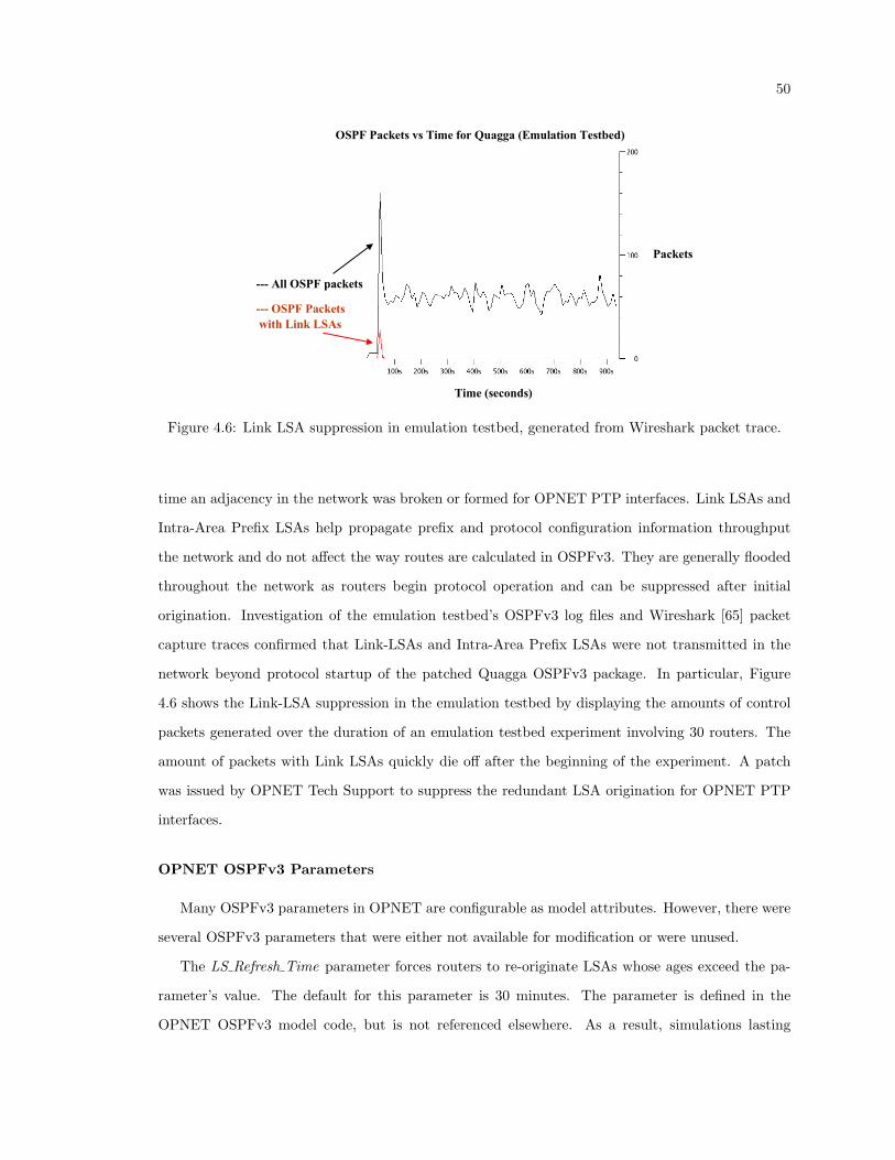
50
Time (seconds)
--- All OSPF packets
--- OSPF Packets
with Link LSAs
Packets
OSPF Packets vs Time for Quagga (Emulation Testbed)
Figure 4.6: Link LSA suppression in emulation testbed, generated from Wireshark packet trace.
time an adjacency in the network was broken or formed for OPNET PTP interfaces. Link LSAs and
Intra-Area Prefix LSAs help propagate prefix and protocol configuration information throughput
the network and do not affect the way routes are calculated in OSPFv3. They are generally flooded
throughout the network as routers begin protocol operation and can be suppressed after initial
origination. Investigation of the emulation testbed’s OSPFv3 log files and Wireshark [65] packet
capture traces confirmed that Link-LSAs and Intra-Area Prefix LSAs were not transmitted in the
network beyond protocol startup of the patched Quagga OSPFv3 package. In particular, Figure
4.6 shows the Link-LSA suppression in the emulation testbed by displaying the amounts of control
packets generated over the duration of an emulation testbed experiment involving 30 routers. The
amount of packets with Link LSAs quickly die off after the beginning of the experiment. A patch
was issued by OPNET Tech Support to suppress the redundant LSA origination for OPNET PTP
interfaces.
OPNET OSPFv3 Parameters
Many OSPFv3 parameters in OPNET are configurable as model attributes. However, there were
several OSPFv3 parameters that were either not available for modification or were unused.
The LS Refresh Time parameter forces routers to re-originate LSAs whose ages exceed the pa-
rameter’s value. The default for this parameter is 30 minutes. The parameter is defined in the
OPNET OSPFv3 model code, but is not referenced elsewhere. As a result, simulations lasting

51
longer than 30 minutes would not include the LSU flooding associated with refreshing older LSAs
(according to the parameter LS Refresh Time).
The MinLSArrival parameter is the maximum rate that routers accept updates for any particular
LSA [59]. In OPNET, this value is fixed to once every 1 second. The MinLSInterval parameter is
the maximum rate that routers will update any particular LSA [59]. OPNET set this value to once
every 5 seconds. These parameters attempt to reduce overhead during turbulent network conditions
that cause frequent LSA changes.
The ability to delay the flooding of LSAs is present in the OPNET MANET interface and was
enabled for the PTP interface by the OPNET Modeler patch (mentioned in Section 4.3.2). This is
known as coalescing of LSAs and is a measure taken to save overhead, by holding back the initial
flooding of LSAs until more LSAs can be packaged into an LSU and sent out together. However,
the method does introduce some amount of delay into the affected packets. Both the MANET and
PTP interfaces in OPNET delay the generation of Router LSAs by 1 second. Finally, the ability to
delay and coalesce LSAck messages is present in both the PTP and MANET interfaces in OPNET.
For MANET interfaces, LSAck messages can be delayed by at most 1 second, while PTP interfaces
can delay acknowledgements up to 1/2 the value of the retransmission interval. A typical value for
the retransmission timer is 5 seconds.
4.4 Creating Equivalent Scenarios
The OPNET scenarios used to validate the emulation testbed were constructed iteratively as
both the simulation and emulation environments were changed and tweaked to match each other.
Experiments on the emulation testbed were conducted for 10 through 30 routers in increments of
5. Overall, scenario construction in OPNET was performed in the same manner for each network
size tested. The issues and challenges involved in establishing equivalent simulation environments
for both tasks are detailed here.
4.4.1 Mobility Matching
Since the emulation testbed consisted of wired routers, a method of emulating node movement
needed to be devised. Devices in a MANET are primarily aware of node mobility only through
changes to the network topology. As nodes move toward and away from each other, the ‘links’
between them go up or down correspondingly. To achieve realistic topology changes in the emulation
52
testbed, traces of node mobility patterns were recorded in OPNET and fed into the emulation
testbed. The information in the traces included node positions and link changes, which listed time,
node pair, and link status change (up, down) at a granularity of 1 second intervals. The link between
nodes was considered ‘up’ if the distance separating them was less than or equal to 250 meters. Note
that the link information passed to the emulation testbed did not include interference levels, as the
emulation testbed did not yet contain functionality for modeling interference.
Each constructed simulation scenario had dimensions of 500 meters by 500 meters. OPNET
mobile nodes of type wlan ethernet router adv were placed in the scenario in the required amounts
(10, 15, 20, 25, 30 routers). Furthermore, nodes were configured to move according to a Random
Waypoint (RWP) mobility model [23] with a constant speed of 20 m/s and pause times of 40 seconds.
Snapshots of network connectivity were withheld until 1800 seconds into the simulation so that the
RWP model could approach steady-state [66] before mobility traces were provided to the emulation
testbed.
4.4.2 Channel Model Matching
The emulation testbed required some compromise from the simulation environment concerning
the physical channel. Routers in the emulation testbed were connected to an Ethernet switch with
1 Gbps links. Transmission delay, propagation delay, and collisions were effectively negligible in
the emulation environment. However, the MANET in the OPNET scenarios consisted of wireless
Institute of Electrical and Electronics Engineers (IEEE) 802.11b routers. As a result, propagation
and transmission delays as well as collisions and retransmissions became significant factors in the
operation of higher layer functions like routing. Functionality to emulate these lower layer effects
was not yet implemented in the emulation testbed, so a second, simpler channel model was used
in the simulation testbed in addition to the standard channel model associated with IEEE 802.11b
radio.
• Standard OPNET Radio Pipeline - The standard OPNET radio pipeline stages compute
received power, interference, Signal to Interference and Noise Ratio (SINR), Bit Error Rate
(BER), bit errors, and error correction. Only a few physical layer parameters were changed
from the defaults set in the wlan ethernet router adv node model. Using the Friis transmission
equation [67] present in the standard radio pipeline stage wlan power.ps.c, it was determined
that, in freespace conditions, a signal transmitted at ∼ 0.25 Watts would be received with a
53
signal strength of −64 dBm at a distance of 250 meters away from the source. Antenna gains
were assumed to be at a default of 0 dB and the transmitted wavelength was calculated from
the center frequency of the first IEEE 802.11b channel. As a result, the transmit power was
changed to 0.25 Watts and the receiver threshold was set to -64 dBm, so that nodes could still
communicate at up to a maximum of 250 meters away from each other.
• Distance-based Radio Pipeline - The distance-based channel model set all of the standard
radio pipeline stages to NONE except for the power, rxgroup, closure, and chanmatch stages.
Packet reception was effectively evaluated using the distance separating the transmitter and
receiver (using the Friis transmission equation [67]), and packet deliveries were performed with-
out delay. Later stages, such as interference, SINR, and BER were ignored. These changes to
the channel model amounted to another step towards more equivalent scenario representation
between the simulation and emulation environments. While simplifying the OPNET channel
model to match the emulation testbed is admittedly worse from a model fidelity point of view,
the procedure was carried out because it is considerably easier to change OPNET models than
to modify the emulation testbed medium access and physical layers. The modifications of the
channel model in OPNET were a sufficient first pass at closing the differences between the
simulation and emulation data link layers, until more advanced emulation features could be
introduced to the testbed.
4.4.3 Network Layer Matching
Experiments on the emulation testbed were conducted for both the modified PTMP and MANET/MDR
interfaces of the patched Quagga OSPFv3. Separate OPNET simulations were conducted with PTP
and PTMP interfaces, both for comparison with the patched Quagga PTMP. Additionally, simu-
lations with OPNET’s MANET interface were compared directly with the patched Quagga MDR
implementation. Most configuration details remained the same regardless of the interface type in
OPNET. OPNET parameters that differ from their default values are listed in Table 4.1.
Additionally, when configuring a PTMP interface in OPNET, each router must be supplied with
a list of neighboring routers, as discussed in Section 4.3.2. Regarding the MANET parameters,
differential Hello messaging and BMDRs were disabled (BMDR flooding is not implemented as
mentioned previously).
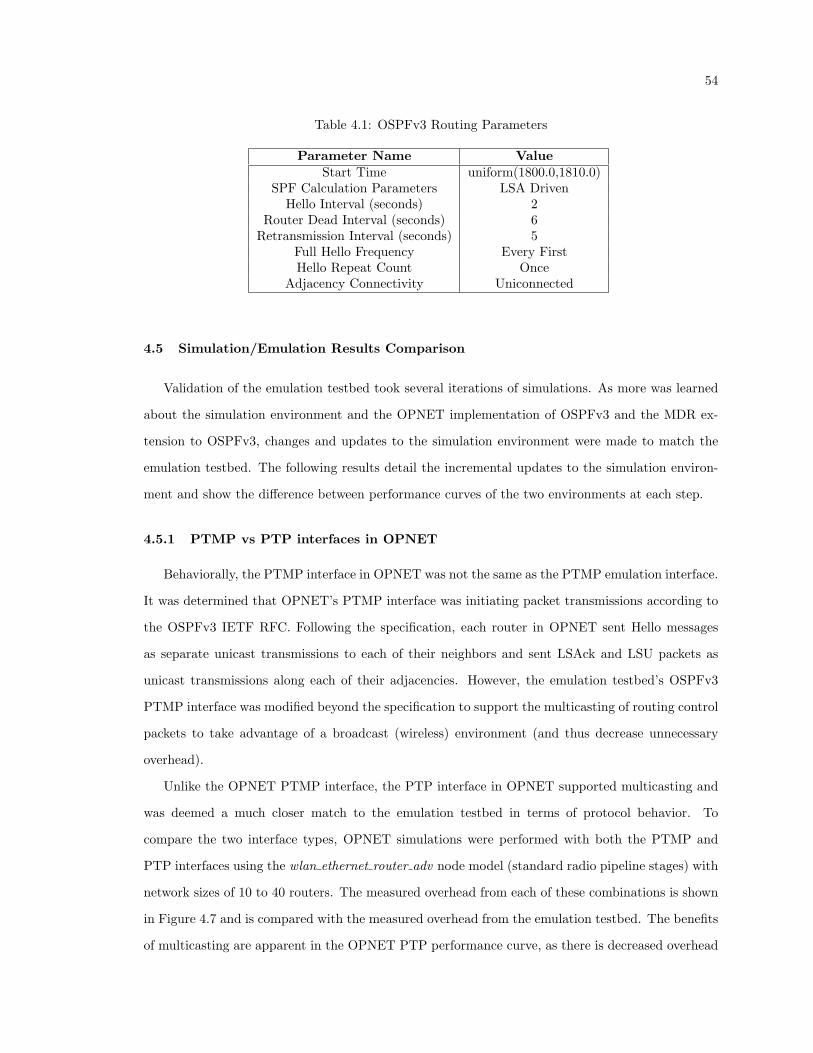
54
Table 4.1: OSPFv3 Routing Parameters
Parameter Name ValueStart Time uniform(1800.0,1810.0)
SPF Calculation Parameters LSA DrivenHello Interval (seconds) 2
Router Dead Interval (seconds) 6Retransmission Interval (seconds) 5
Full Hello Frequency Every FirstHello Repeat Count Once
Adjacency Connectivity Uniconnected
4.5 Simulation/Emulation Results Comparison
Validation of the emulation testbed took several iterations of simulations. As more was learned
about the simulation environment and the OPNET implementation of OSPFv3 and the MDR ex-
tension to OSPFv3, changes and updates to the simulation environment were made to match the
emulation testbed. The following results detail the incremental updates to the simulation environ-
ment and show the difference between performance curves of the two environments at each step.
4.5.1 PTMP vs PTP interfaces in OPNET
Behaviorally, the PTMP interface in OPNET was not the same as the PTMP emulation interface.
It was determined that OPNET’s PTMP interface was initiating packet transmissions according to
the OSPFv3 IETF RFC. Following the specification, each router in OPNET sent Hello messages
as separate unicast transmissions to each of their neighbors and sent LSAck and LSU packets as
unicast transmissions along each of their adjacencies. However, the emulation testbed’s OSPFv3
PTMP interface was modified beyond the specification to support the multicasting of routing control
packets to take advantage of a broadcast (wireless) environment (and thus decrease unnecessary
overhead).
Unlike the OPNET PTMP interface, the PTP interface in OPNET supported multicasting and
was deemed a much closer match to the emulation testbed in terms of protocol behavior. To
compare the two interface types, OPNET simulations were performed with both the PTMP and
PTP interfaces using the wlan ethernet router adv node model (standard radio pipeline stages) with
network sizes of 10 to 40 routers. The measured overhead from each of these combinations is shown
in Figure 4.7 and is compared with the measured overhead from the emulation testbed. The benefits
of multicasting are apparent in the OPNET PTP performance curve, as there is decreased overhead
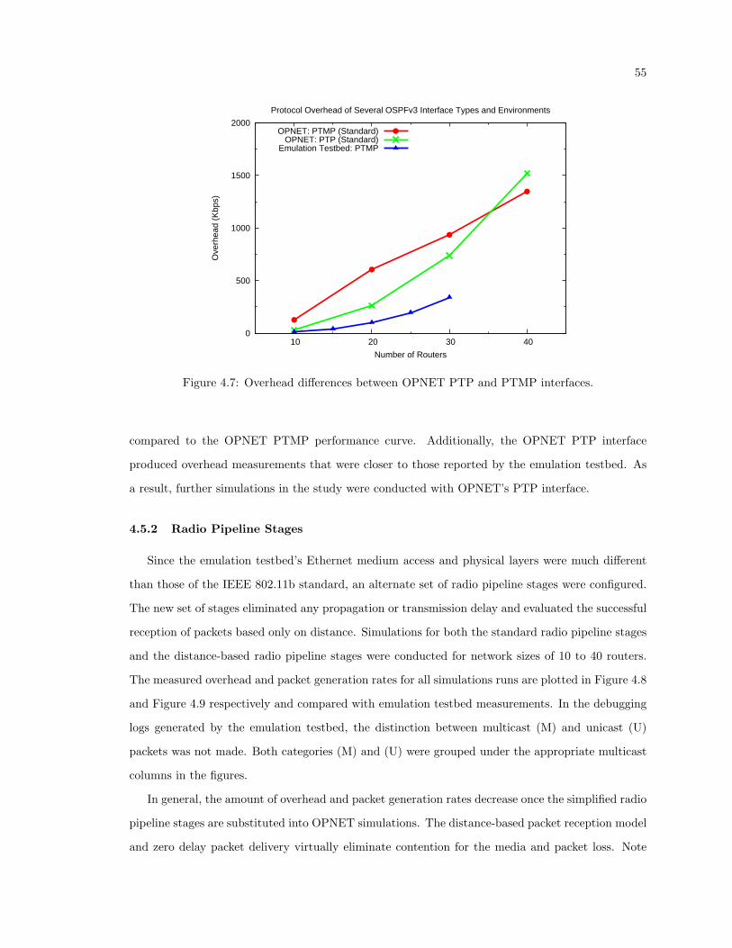
55
0
500
1000
1500
2000
10 20 30 40
Ove
rhea
d (K
bps)
Number of Routers
Protocol Overhead of Several OSPFv3 Interface Types and Environments
OPNET: PTMP (Standard)OPNET: PTP (Standard)
Emulation Testbed: PTMP
Figure 4.7: Overhead differences between OPNET PTP and PTMP interfaces.
compared to the OPNET PTMP performance curve. Additionally, the OPNET PTP interface
produced overhead measurements that were closer to those reported by the emulation testbed. As
a result, further simulations in the study were conducted with OPNET’s PTP interface.
4.5.2 Radio Pipeline Stages
Since the emulation testbed’s Ethernet medium access and physical layers were much different
than those of the IEEE 802.11b standard, an alternate set of radio pipeline stages were configured.
The new set of stages eliminated any propagation or transmission delay and evaluated the successful
reception of packets based only on distance. Simulations for both the standard radio pipeline stages
and the distance-based radio pipeline stages were conducted for network sizes of 10 to 40 routers.
The measured overhead and packet generation rates for all simulations runs are plotted in Figure 4.8
and Figure 4.9 respectively and compared with emulation testbed measurements. In the debugging
logs generated by the emulation testbed, the distinction between multicast (M) and unicast (U)
packets was not made. Both categories (M) and (U) were grouped under the appropriate multicast
columns in the figures.
In general, the amount of overhead and packet generation rates decrease once the simplified radio
pipeline stages are substituted into OPNET simulations. The distance-based packet reception model
and zero delay packet delivery virtually eliminate contention for the media and packet loss. Note
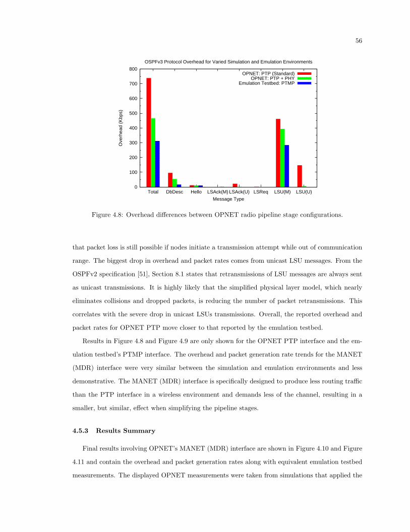
56
0
100
200
300
400
500
600
700
800
LSU(U)LSU(M)LSReqLSAck(U)LSAck(M)HelloDbDescTotal
Ove
rhea
d (K
bps)
Message Type
OSPFv3 Protocol Overhead for Varied Simulation and Emulation Environments
OPNET: PTP (Standard)OPNET: PTP + PHY
Emulation Testbed: PTMP
Figure 4.8: Overhead differences between OPNET radio pipeline stage configurations.
that packet loss is still possible if nodes initiate a transmission attempt while out of communication
range. The biggest drop in overhead and packet rates comes from unicast LSU messages. From the
OSPFv2 specification [51], Section 8.1 states that retransmissions of LSU messages are always sent
as unicast transmissions. It is highly likely that the simplified physical layer model, which nearly
eliminates collisions and dropped packets, is reducing the number of packet retransmissions. This
correlates with the severe drop in unicast LSUs transmissions. Overall, the reported overhead and
packet rates for OPNET PTP move closer to that reported by the emulation testbed.
Results in Figure 4.8 and Figure 4.9 are only shown for the OPNET PTP interface and the em-
ulation testbed’s PTMP interface. The overhead and packet generation rate trends for the MANET
(MDR) interface were very similar between the simulation and emulation environments and less
demonstrative. The MANET (MDR) interface is specifically designed to produce less routing traffic
than the PTP interface in a wireless environment and demands less of the channel, resulting in a
smaller, but similar, effect when simplifying the pipeline stages.
4.5.3 Results Summary
Final results involving OPNET’s MANET (MDR) interface are shown in Figure 4.10 and Figure
4.11 and contain the overhead and packet generation rates along with equivalent emulation testbed
measurements. The displayed OPNET measurements were taken from simulations that applied the
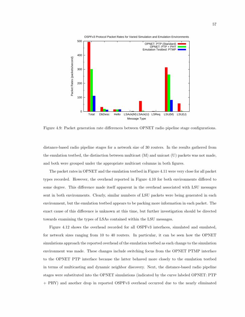
57
0
100
200
300
400
500
LSU(U)LSU(M)LSReqLSAck(U)LSAck(M)HelloDbDescTotal
Pac
ket R
ates
(pa
cket
s/se
cond
)
Message Type
OSPFv3 Protocol Packet Rates for Varied Simulation and Emulation Environments
OPNET: PTP (Standard)OPNET: PTP + PHY
Emulation Testbed: PTMP
Figure 4.9: Packet generation rate differences between OPNET radio pipeline stage configurations.
distance-based radio pipeline stages for a network size of 30 routers. In the results gathered from
the emulation testbed, the distinction between multicast (M) and unicast (U) packets was not made,
and both were grouped under the appropriate multicast columns in both figures.
The packet rates in OPNET and the emulation testbed in Figure 4.11 were very close for all packet
types recorded. However, the overhead reported in Figure 4.10 for both environments differed to
some degree. This difference made itself apparent in the overhead associated with LSU messages
sent in both environments. Clearly, similar numbers of LSU packets were being generated in each
environment, but the emulation testbed appears to be packing more information in each packet. The
exact cause of this difference is unknown at this time, but further investigation should be directed
towards examining the types of LSAs contained within the LSU messages.
Figure 4.12 shows the overhead recorded for all OSPFv3 interfaces, simulated and emulated,
for network sizes ranging from 10 to 40 routers. In particular, it can be seen how the OPNET
simulations approach the reported overhead of the emulation testbed as each change to the simulation
environment was made. These changes include switching focus from the OPNET PTMP interface
to the OPNET PTP interface because the latter behaved more closely to the emulation testbed
in terms of multicasting and dynamic neighbor discovery. Next, the distance-based radio pipeline
stages were substituted into the OPNET simulations (indicated by the curve labeled OPNET: PTP
+ PHY) and another drop in reported OSPFv3 overhead occurred due to the nearly eliminated
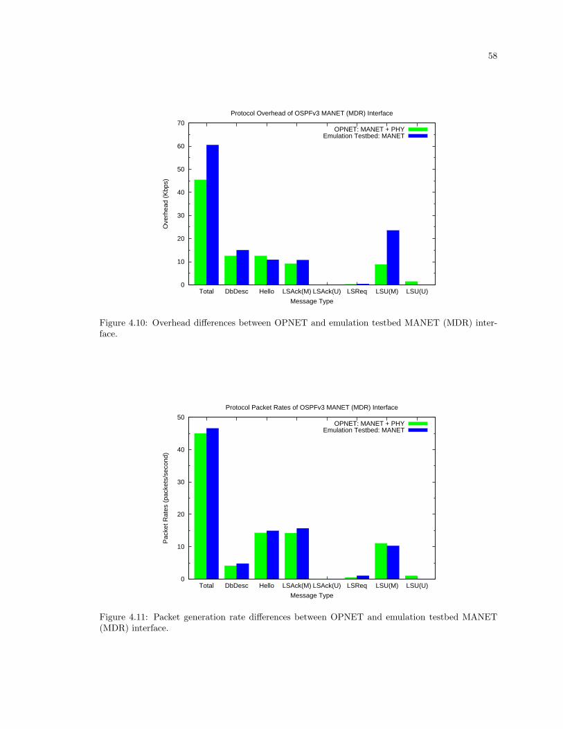
58
0
10
20
30
40
50
60
70
LSU(U)LSU(M)LSReqLSAck(U)LSAck(M)HelloDbDescTotal
Ove
rhea
d (K
bps)
Message Type
Protocol Overhead of OSPFv3 MANET (MDR) Interface
OPNET: MANET + PHYEmulation Testbed: MANET
Figure 4.10: Overhead differences between OPNET and emulation testbed MANET (MDR) inter-face.
0
10
20
30
40
50
LSU(U)LSU(M)LSReqLSAck(U)LSAck(M)HelloDbDescTotal
Pac
ket R
ates
(pa
cket
s/se
cond
)
Message Type
Protocol Packet Rates of OSPFv3 MANET (MDR) Interface
OPNET: MANET + PHYEmulation Testbed: MANET
Figure 4.11: Packet generation rate differences between OPNET and emulation testbed MANET(MDR) interface.
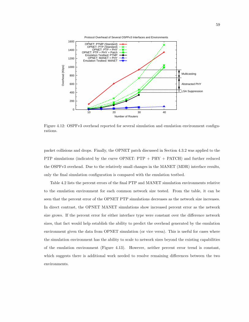
59
0
200
400
600
800
1000
1200
1400
1600
10 20 30 40
Ove
rhea
d (K
bps)
Number of Routers
Protocol Overhead of Several OSPFv3 Interfaces and Environments
Multicasting
Abstracted PHY
LSA Suppression
OPNET: PTMP (Standard)OPNET: PTP (Standard)
OPNET: PTP + PHYOPNET: PTP + PHY + Patch
Emulation Testbed: PTMPOPNET: MANET + PHY
Emulation Testbed: MANET
Figure 4.12: OSPFv3 overhead reported for several simulation and emulation environment configu-rations.
packet collisions and drops. Finally, the OPNET patch discussed in Section 4.3.2 was applied to the
PTP simulations (indicated by the curve OPNET: PTP + PHY + PATCH) and further reduced
the OSPFv3 overhead. Due to the relatively small changes in the MANET (MDR) interface results,
only the final simulation configuration is compared with the emulation testbed.
Table 4.2 lists the percent errors of the final PTP and MANET simulation environments relative
to the emulation environment for each common network size tested. From the table, it can be
seen that the percent error of the OPNET PTP simulations decreases as the network size increases.
In direct contrast, the OPNET MANET simulations show increased percent error as the network
size grows. If the percent error for either interface type were constant over the difference network
sizes, that fact would help establish the ability to predict the overhead generated by the emulation
environment given the data from OPNET simulation (or vice versa). This is useful for cases where
the simulation environment has the ability to scale to network sizes beyond the existing capabilities
of the emulation environment (Figure 4.13). However, neither percent error trend is constant,
which suggests there is additional work needed to resolve remaining differences between the two
environments.
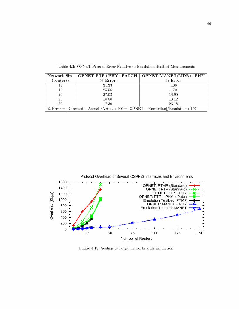
60
Table 4.2: OPNET Percent Error Relative to Emulation Testbed Measurements
Network Size OPNET PTP+PHY+PATCH OPNET MANET(MDR)+PHY(routers) % Error % Error
10 31.33 4.8015 25.56 1.7020 27.02 18.9025 18.80 18.1230 17.30 26.18
% Error = |Observed−Actual|/Actual ∗ 100 = |OPNET− Emulation|/Emulation ∗ 100
0
200
400
600
800
1000
1200
1400
1600
25 50 75 100 125 150
Ove
rhea
d (K
bps)
Number of Routers
Protocol Overhead of Several OSPFv3 Interfaces and Environments
OPNET: PTMP (Standard)OPNET: PTP (Standard)
OPNET: PTP + PHYOPNET: PTP + PHY + Patch
Emulation Testbed: PTMPOPNET: MANET + PHY
Emulation Testbed: MANET
Figure 4.13: Scaling to larger networks with simulation.
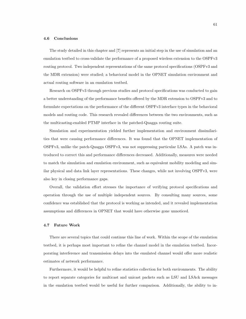
61
4.6 Conclusions
The study detailed in this chapter and [7] represents an initial step in the use of simulation and an
emulation testbed to cross-validate the performance of a proposed wireless extension to the OSPFv3
routing protocol. Two independent representations of the same protocol specifications (OSPFv3 and
the MDR extension) were studied; a behavioral model in the OPNET simulation environment and
actual routing software in an emulation testbed.
Research on OSPFv3 through previous studies and protocol specifications was conducted to gain
a better understanding of the performance benefits offered by the MDR extension to OSPFv3 and to
formulate expectations on the performance of the different OSPFv3 interface types in the behavioral
models and routing code. This research revealed differences between the two environments, such as
the multicasting-enabled PTMP interface in the patched-Quagga routing suite.
Simulation and experimentation yielded further implementation and environment dissimilari-
ties that were causing performance differences. It was found that the OPNET implementation of
OSPFv3, unlike the patch-Quagga OSPFv3, was not suppressing particular LSAs. A patch was in-
troduced to correct this and performance differences decreased. Additionally, measures were needed
to match the simulation and emulation environment, such as equivalent mobility modeling and sim-
ilar physical and data link layer representations. These changes, while not involving OSPFv3, were
also key in closing performance gaps.
Overall, the validation effort stresses the importance of verifying protocol specifications and
operation through the use of multiple independent sources. By consulting many sources, some
confidence was established that the protocol is working as intended, and it revealed implementation
assumptions and differences in OPNET that would have otherwise gone unnoticed.
4.7 Future Work
There are several topics that could continue this line of work. Within the scope of the emulation
testbed, it is perhaps most important to refine the channel model in the emulation testbed. Incor-
porating interference and transmission delays into the emulated channel would offer more realistic
estimates of network performance.
Furthermore, it would be helpful to refine statistics collection for both environments. The ability
to report separate categories for multicast and unicast packets such as LSU and LSAck messages
in the emulation testbed would be useful for further comparison. Additionally, the ability to in-
62
vestigate the type and amount of specific types of LSAs being packaged into LSUs would be very
helpful in continuing the investigation of remaining differences between the emulation and simulation
environments.
If the MANET (MDR) extension of OSPFv3 is to be studied further, it would be useful to have
more LSAFullness options and BMDR flooding built into the OPNET implementation. In this
study, testing of the MANET interface was rather limited due to the lack of options in OPNET’s
implementation.
Finally, ways to extend this study include modeling application traffic on top of the routing pro-
tocol. This would open the ability to study performance metrics such as packet delivery percentage
and packet latency among others. Another important branch from this study includes modeling and
emulating the other proposed OSPFv3 wireless extensions.
63
5. Conclusions
This body of work presented three case studies that a.) highlight issues affecting the use of
simulation as well as b) detail ways of applying simulation to the study of wireless networking
protocols.
The performance of simulators, measured in both accuracy of results and run time, is a constant
concern to simulation users. Chapter 2 developed three abstractions of the IEEE 802.11 RTS/CTS
channel access mechanism in order to combat prohibitively high running times in simulations of
large scale mobile ad hoc networks. The design of the abstractions sought to decrease scaling of
simulation runtime with network size by combining events and reducing the number of receivers
considered for physical layer calculations for control frames. Each level of abstraction did manage
to improve on the run time required to complete a simulation. In particular, the ‘best’ abstraction
was the Simplified Neighbor List which achieved near-linear scaling.
Simulations of the abstracted models yielded goodput results that were very comparable to those
of the OPNET validation model, but contained some discrepancy in the data trends for ETE delay
measurements. This discrepancy is likely rooted in the fact that all three abstractions compressed
RTS and CTS events together into an instantaneous transmission, which would have a direct effect
on time-based metrics such as ETE delay. Future work with RTS/CTS abstraction includes studying
additional abstraction methods to developing the notion that different forms of protocol abstraction
are best suited for collecting particular data. Such a study would attempt to yield guidelines in
choosing the best abstraction model given a desired metric.
Chapter 3 examined the feasibility of a new protocol via simulation, before involving the costs
of any testbed hardware. A literature survey of autoconfiguration schemes designed for MANETs
was provided, with particular focus on a stateless autoconfiguration scheme by Jelger and Noel
(SECON 2005). The selected scheme provides globally routable IPv6 prefixes to a MANET at-
tached to the Internet via gateways. Initially, the OPNET protocol model was validated against
the original authors’ data to ensure proper operation. Discussion with the J&N protocol authors
revealed simulation setup differences as potential sources for differences in prefix hold times in the
validation scenario.
The Jelger-Noel scheme was also examined with new cluster mobility models, added gateway
mobility, and varied network sizes. Performance of the Jelger-Noel scheme, derived from overhead,
64
autoconfiguration time and prefix stability metrics, was found to be highly dependent on network
density. Low prefix hold time measurements were noted, and it was suggested that ad hoc nodes may
experience difficulties in maintaining higher layer sessions. The J&N protocol may need be revised
further to improve performance in this area. Areas of future work include investigating potential
tradeoffs between prefix hold times and percentage of time without a prefix, controlled by network
density.
Finally, in Chapter 4, simulations cross-validated an emulation testbed running the Open Shortest
Path First (OSPF) routing protocol and its MANET Designated Router (MDR) extension. Proto-
col specifications and previous OSPF studies were researched to gain a better understanding of the
performance benefits offered by the MDR extension to OSPFv3, and to develop performance expec-
tations in both the simulator’s behavioral code and the emulation testbed’s protocol implementation.
This research revealed differences between the two environments, such as the multicasting-enabled
PTMP interface in the patched-Quagga routing suite. The measured OSPF overhead and packet
rates from both environments was used as a benchmark to construct equivalent MANET represen-
tations and protocol configuration, made particularly challenging due to the wired nature of the
emulation testbed.
During the process of performance matching, simulation and experimentation yielded further
implementation and environment dissimilarities that were causing performance differences. It was
found that the OPNET implementation of OSPFv3, unlike the patch-Quagga OSPFv3, was not
suppressing particular LSAs. A patch was introduced to OPNET to correct this and performance
differences decreased. Additionally, measures were needed to match the simulation and emulation
environment, such as equivalent mobility modeling and similar physical and data link layer repre-
sentations. These changes, while not involving OSPFv3, were also key in closing performance gaps.
Overall, both validation efforts in the study stressed the importance of verifying protocol specifica-
tions and operation through the use of multiple independent sources. By cross-validating simulation
and emulation data, the simulation’s OSPF model limitations were revealed, and confidence was
established that the protocol is configured and working as intended in the emulation testbed.

66
Bibliography
[1] L. Breslau, D. Estrin, K. Fall, S. Floyd, J. Heidemann, A. Helmy, P. Huang, S. McCanne,K. Varadhan, Y. Xu, and H. Yu, “Advances in network simulation,” IEEE Computer, vol. 33,pp. 59–67, May 2000.
[2] B. Blum, T. He, and Y. Pointurier, “MAC layer abstraction for simulation scalability improve-ments.” Computer Science Department, University of Virginia, December 2001.
[3] P. Zheng and L. M. Ni, “Empower: A scalable framework for network emulation,” in Proceedingsof the 31th Annual IEEE International Conference on Parallel Processing (ICPP ’02), pp. 185–192, August 2002. Vancouver, British Columbia, Canada.
[4] J. Wildman, B. Willman, M. Kirkpatrick, and S. Weber, “RTS/CTS data link abstractions formobile ad hoc networks,” in Proceedings of the 25th Annual IEEE Military CommunicationsConference (MILCOM ’06), October 2006. Washington, DC, USA.
[5] C. Jelger and T. Noel, “Proactive address autoconfiguration and prefix continuity in IPv6 hybridad hoc networks,” in Proceedings of the 2nd Annual IEEE Sensor and Ad Hoc Communicationsand Networks Conference (SECON ’05), pp. 107–117, September 2005. Santa Clara, CA, USA.
[6] J. Wildman, D. Hamel, R. Measel, D. Oakum, S. Weber, and M. Kam, “Performance andscaling of wireless ad hoc IPv6 stateless address autoconfiguration under mobile gateways,” inProceedings of the 26th Annual IEEE Military Communications Conference (MILCOM ’07),October 2007. Orlando, FL, USA.
[7] G. Carl, S. Dastangoo, and J. Wildman, “Using an emulation testbed to measure OSPF routingoverhead due to mobility in wireless ad hoc networks,” in Proceedings of the 27th Annual IEEEMilitary Communications Conference (MILCOM ’08), November 2008. San Diego, CA, USA.
[8] V. Naoumov and T. Gross, “Simulation of large ad hoc networks,” in Proceedings of the 6thAnnual ACM International Workshop on Modeling Analysis and Simulation of Wireless andMobile Systems (MSWiM ’03), pp. 50–57, September 2003. San Diego, CA, USA.
[9] “OPNET modeler.” Online: http://www.opnet.com/.
[10] X. J. Liu, Improvements in Conservative Parallel Simulation of Large-scale Models. PhD thesis,Dartmouth College, Hanover, NH, USA, February 2003.
[11] C. Liu, M. A. Orgun, and K. Zhang, “A parallel execution model for Chronolog,” InternationalJournal of Computer Systems Science and Engineering, vol. 16, no. 4, 2001.
[12] M. Takai, R. Bagrodia, A. Lee, and M. Gerla, “Impact of channel models on simulation of largescale wireless networks,” in Proceedings of the 2nd Annual ACM International Workshop onModeling Analysis and Simulation of Wireless and Mobile Systems (MSWiM ’99), pp. 7–14,1999.
[13] T. He, B. Blum, Y. Pointurier, C. Lu, J. A. Stankovic, and S. Son, “MAC layer abstractionfor simulation scalability improvements in large-scale sensor networks,” in Proceedings of the3rd Annual International Conference on Networked Sensing Systems (INSS ’06), TransducerResearch Foundation (TRF), May 2006. Chicago, IL, USA.
[14] J. Heidemann, N. Bulusu, J. Elson, C. Intanagonwiwat, K. Lan, Y. Xu, W. Ye, D. Estrin,and R. Govindan, “Effects of detail in wireless network simulation,” in Proceedings of the SCSMulticonference on Distributed Simulation, pp. 3–11, Society for Computer Simulation (SCS),January 2001.
67
[15] M. Takai, J. Martin, and R. Bagrodia, “Effects of wireless physical layer modeling in mobilead hoc networks,” in Proceedings of the 2nd Annual ACM International Symposium on MobileAd Hoc Networking and Computing (MobiHoc ’01), pp. 87–94, October 2001. Long Beach, CA,USA.
[16] M. Pidd, “Five simple principles of modelling,” in Proceedings of the 1996 Winter SimulationConference (WSC ’96), pp. 721–728, December 1996. Coronado, CA, USA.
[17] D. D. Cavin, Y. Sasson, and A. Schiper, “On the accuracy of MANET simulators,” in Pro-ceedings of the 2nd Annual ACM Workshop on Principles of Mobile Computing (POMC’02),pp. 38–43, October 2002. Toulouse, France.
[18] L. F. Perrone and D. M. Nicol, “Using n-body algorithms for interference computation in wire-less cellular simulations,” in Proceedings of the 8th Annual IEEE International Symposium onModeling, Analysis and Simulation of Computer and Telecommunication Systems (MASCOTS’00), pp. 49–56, August 2000. San Francisco, CA, USA.
[19] J. Liu, D. M. Nicol, L. F. Perrone, and M. Liljenstam, “Towards high performance modeling ofthe 802.11 wireless protocol,” in Proceedings of the 2001 Winter Simulation Conference (WSC’01), vol. 2, pp. 1315–1320, December 2001. Arlington, VA, USA.
[20] L. C. Zhong and J. M. Rabaey, “Modeling and analysis of the data link layer in wireless sensornetworks.” Berkeley Wireless Research Center, Department of EECS, University of Califor-nia at Berkeley. Online: http://bwrc.eecs.berkeley.edu/People/Grad_Students/czhong/restricted/ICC2003.pdf.
[21] N. Golmie, R. E. Van Dyck, and A. Soltanian, “Interference of Bluetooth and IEEE 802.11:Simulation modeling and performance evaluation,” in Proceedings of the 4th Annual ACM In-ternational Workshop on Modeling, Analysis and Simulation of Wireless and Mobile Systems(MSWiM ’01), pp. 11–18, July 2001. Rome, Italy.
[22] A. Heindl and R. German, “Performance modeling of IEEE 802.11 wireless LANs with stochasticPetri nets,” Performance Evaluation, vol. 44, pp. 139–164, April 2001.
[23] T. Camp, J. Boleng, and V. Davies, “A survey of mobility models for ad hoc network research,”Wireless Communications and Mobile Computing, vol. 2, no. 5, pp. 483–502, 2002.
[24] J. Yoon, M. Liu, and B. Noble, “Random waypoint considered harmful,” in Proceedings ofthe 22nd Annual IEEE Conference on Computer Communications (INFOCOM ’03), vol. 2,pp. 1312–1321, March 2003. San Francisco, CA, USA.
[25] C. S. R. Murthy and B. S. Manoj, Ad Hoc Wireless Networks: Architectures and Protocols.Prentice Hall Professional Technical Reference, 2004.
[26] “Part 11: Wireless (LAN) medium access control (MAC) and physical layer (PHY) specifica-tions,” ANSI/IEEE Std 802.11, 1999 Edition (R2003), 2003.
[27] C. E. Perkins, J. T. Malinen, R. Wakikawa, E. M. Belding-Royer, and Y. Sun, “IP addressautoconfiguration for ad hoc networks.” Internet Draft (work in progress) draft-perkins-manet-autoconf-01.txt, IETF, November 2001.
[28] N. H. Vaidya, “Weak duplicate address detection in mobile ad hoc networks,” in Proceedings ofthe 3rd Annual ACM International Symposium on Mobile Ad Hoc Networking and Computing(MobiHoc ’02), pp. 206–216, June 2002. Lausanne, Switzerland.
[29] K. Weniger, “Passive duplicate address detection in mobile ad hoc networks,” in Proceedings ofthe Annual IEEE Wireless Communications and Networking Conference (WCNC ’03), vol. 3,pp. 1504–1509, March 2003. New Orleans, LA, USA.
68
[30] Y. Sun and E. M. Belding-Royer, “A study of dynamic addressing techniques in mobile ad hocnetworks,” Wireless Communications and Mobile Computing, vol. 4, pp. 315–329, April 2004.
[31] K. Weniger, “PACMAN: Passive autoconfiguration for mobile ad-hoc networks,” IEEE Journalon Selected Areas in Communications, vol. 23, pp. 507–519, March 2005.
[32] B. Wehbi, “Address autoconfiguration in ad hoc networks.” Internal Report, Departement Logi-ciels Reseaux, Institute National des Telecommunications. Online: http://www.bachwehbi.net/autoconf_report.pdf, May 2005.
[33] K. Weniger and M. Zitterbart, “Address autoconfiguration in mobile ad hoc networks: Currentapproaches and future directions,” IEEE Network, vol. 18, pp. 6–11, August 2004.
[34] L. Lamont, M. Wang, L. Villasenor, T. Randhawa, and S. Hardy, “Integrating WLANs andMANETs to the IPv6 based Internet,” in Proceedings of the 38th Annual IEEE InternationalConference on Communications (ICC ’03), vol. 2, pp. 1090–1095, May 2003. Anchorage, AK,USA.
[35] C.-Y. Wang, C.-Y. Li, R.-H. Hwang, and Y.-S. Chen, “Global connectivity for mobile IPv6-based ad hoc networks,” in Proceedings of the 19th Annual IEEE International Conference onAdvanced Information Networking and Applications (AINA ’05), vol. 2, pp. 807–812, March2005. Taipei, Taiwan.
[36] M. Gunes and J. Reibel, “An IP address configuration algorithm for zeroconf mobile multihopad hoc networks,” in Proceedings of the International Workshop on Broadband Wireless Ad HocNetworks and Services, September 2002. Sophia Antipolis, France.
[37] S. Nesargi and R. Prakash, “MANETconf: Configuration of hosts in a mobile ad hoc network,”in Proceedings of the 21st Annual IEEE Conference on Computer Communications (INFOCOM’02), vol. 2, pp. 1059–1068, June 2002. New York, NY, USA.
[38] M. Bagnulo, I. Soto, A. Garcia-Martinez, and A. Azcorra, “Random generation of interface iden-tifiers.” Internet Draft (work in progress) draft-soto-mobileip-randim-iids-00.txt, IETF, January2002.
[39] K. S. King and N. Smith, “Dynamic addressing and mobility in tactical hybrid ad hoc networks,”in Proceedings of the 24th Annual IEEE Military Communications Conference (MILCOM ’05),vol. 5, pp. 2930–2935, October 2005. Atlantic City, NJ, USA.
[40] H. Ammari and H. El-Rewini, “Integration of mobile ad hoc networks and the Internet using mo-bile gateways,” in Proceedings of the 18th Annual IEEE International Parallel and DistributedProcessing Symposium (IPDPS ’04), pp. 218–225, April 2004. Santa Fe, NM, USA.
[41] M. K. Denko and C. Wei, “An architecture for integrating mobile ad hoc networks with theInternet using multiple mobile gateways,” in Proceedings of the 18th Annual IEEE CanadianConference on Electrical and Computer Engineering (CCECE ’05), pp. 1097–1102, May 2005.Saskatchewan, Canada.
[42] Y. Mo, J. Huang, and B. Huang, “MANET node based mobile gateway with unspecific MANETrouting protocol,” in Proceedings of the 6th Annual IEEE International Symposium on Com-munications and Information Technologies (ISCIT ’06), pp. 886–889, October 2006. Bangkok,Thailand.
[43] D. B. Green, “Stryker brigade combat team IPv6 transition modeling and simulation study,”in Proceedings of the 24th Annual IEEE Military Communications Conference (MILCOM ’05),vol. 4, pp. 2275–2281, October 2005. Atlantic City, NJ, USA.
69
[44] L. Kant, F. Anjum, and K. Young, “Design and analysis of scalable network centric warfaremechanisms,” in Proceedings of the 25th Army Science Conference (ASC ’06), November 2006.
[45] C. Jelger, T. Noel, and A. Frey, “Gateway and address autoconfiguration for IPv6 ad hoc net-works.” Internet Draft (work in progress) draft-jelger-manet-gateway-autoconf-v6-02.txt, IETF,April 2004.
[46] A. Frey, “Autoconfiguration in IPv6 wireless ad hoc networks - stand alone daemon,” Oc-tober 2004. Online: http://www-r2.u-strasbg.fr/~frey/safari/autoconf.html, accessedAugust 23, 2008.
[47] C. Jelger, Gestion des equipments mobiles et communications de group dans l’Internet NouvelleGeneration. PhD thesis, Universite Louis Pasteur, Strasbourg, France, October 2004. (inFrench).
[48] M. Chandra and A. Roy (eds.), “Extensions to ospf to support mobile ad hoc networking.”Internet Draft (work in progress) draft-ietf-ospf-manet-or-00.txt, IETF, February 2008.
[49] R. Ogier and P. Spagnolo, “MANET extension of OSPF using CDS flooding.” Internet Draft(work in progress) draft-ietf-ospf-manet-mdr-02.txt, IETF, June 2008.
[50] E. Bacelli, P. Jacquet, D. Nguyen, and T. Clausen, “OSPF MPR extension for ad hoc networks.”Internet Draft (work in progress) draft-ietf-ospf-manet-mpr-01.txt, IETF, July 2008.
[51] J. Moy, “OSPF version 2,” April 1998. Request for Comments 2328, IETF.
[52] R. Coltun, D. Ferguson, and J. Moy, “OSPF for IPv6,” December 1999. Request for Comments2740, IETF.
[53] R. Coltun, D. Ferguson, J. Moy, and A. Lindem (ed.), “OSPF for IPv6,” July 2008. Requestfor Comments 5340, IETF.
[54] Z. J. Haas, “Panel report on ad hoc networks - MILCOM ’97,” ACM SIGMOBILE MobileComputing and Communications Review, vol. 2, pp. 15–18, January 1998.
[55] T. R. Henderson, P. A. Spagnolo, and J. H. Kim, “A wireless interface type for OSPF,” inProceedings of the 22nd Annual IEEE Military Communications Conference (MILCOM ’03),vol. 2, pp. 1256–1261, October 2003. Boston, MA, USA.
[56] M. Chandra (ed.), “Extensions to OSPF to support mobile ad hoc networking.” Internet Draft(work in progress) draft-chandra-ospf-manet-ext-03.txt, IETF, April 2005.
[57] R. Ogier and P. Spagnolo, “MANET extension of OSPF using CDS flooding.” Internet Draft(work in progress) draft-ogier-manet-ospf-extension-04.txt, IETF, July 2005.
[58] T. R. Henderson, P. A. Spagnolo, and G. Pei, “Evaluation of OSPF MANET extensions,” Tech.Rep. D950-10987-1, Boeing, July 2005. Online: http://hipserver.mct.phantomworks.org/ietf/ospf.
[59] J. T. Moy, OSPF: Anatomy of an Internet Routing Protocol. Reading, MA, USA: Addison-Wesley, 1998.
[60] J. T. Moy, OSPF: Complete Implementation. Reading, MA, USA: Addison-Wesley, 2001.
[61] J. Doyle and J. Carroll, Routing TCP/IP, vol. 1 of CCIE Professional Development. Indianapo-lis, IN, USA: Cisco Press, 2nd ed., 2006.
[62] P. A. Spagnolo and T. R. Henderson, “Comparison of proposed OSPF MANET extensions,”in Proceedings of the 25th Annual IEEE Military Communications Conference (MILCOM ’06),October 2006. Washington, DC, USA.

70
[63] “Quagga software routing suite.” Online: http://www.quagga.net/.
[64] R. Ogier and P. Spagnolo, “MANET extension of OSPF using CDS flooding.” Internet Draft(work in progress) draft-ogier-manet-ospf-extension-06.txt, IETF, December 2005.
[65] “Wireshark: Network protocol analyzer.” Online: http://www.wireshark.org/.
[66] C. Bettstetter, G. Resta, and P. Santi, “The node distribution of the random waypoint mobilitymodel for wireless ad hoc networks,” IEEE Transactions on Mobile Computing, vol. 2, pp. 257–269, July-September 2003.
[67] W. Ye, Radio Propagation Models. in ns Manual, Online: http://www.isi.edu/~weiye/pub/propagation_ns.pdf.

71
Appendix A. RTS/CTS Sequence Pseudocode
A.1 Event Compression
Procedure 1 Event-Compression RTS/CTS1: upon node s is IDLE and has frame to send to node d2: set rts flag = false3: set cts flag = false4: retrieve entire set of nodes, L5: for every node i in L such that i 6= s do6: compute transmission attempt from s to i7: if attempt == valid then8: if i == d then9: set rts flag = true
10: else11: NAV/backoff timer of i adjusted12: if rts flag == true then13: for every node i in L such that i 6= d do14: compute transmission attempt from d to i15: if attempt == valid then16: if i == s then17: set cts flag = true18: else19: NAV/backoff timer of i adjusted20: if (rts flag == true)&(cts flag == true) then21: proceed to original frame transmission22: else23: backoff and attempt later

72
A.2 Neighbor List
Procedure 2 Neighbor List RTS/CTS1: upon node s is IDLE and has frame to send to node d2: set rts flag = false3: set cts flag = false4: retrieve neighbor list, nls, of node s5: for every node i in nls such that i 6= s do6: compute transmission attempt from s to i7: if attempt == valid then8: if i == d then9: set rts flag = true
10: else11: NAV/backoff timer of i adjusted12: if rts flag == true then13: retrieve neighbor list, nld, of node d14: for every node i in nld such that i 6= d do15: compute transmission attempt from d to i16: if attempt == valid then17: if i == s then18: set cts flag = true19: else20: NAV/backoff timer of i adjusted21: if (rts flag == true)&(cts flag == true) then22: proceed to original frame transmission23: else24: backoff and attempt later

73
A.3 Simplified Neighbor List
Procedure 3 Simplified Neighbor List RTS/CTS1: upon node s is IDLE and has frame to send to node d2: set rts flag = false3: set cts flag = false4: retrieve neighbor list, nls, of node s5: for every node i in nls such that i 6= s do6: if i == d then7: compute transmission attempt from s to d8: if attempt == valid then9: set rts flag = true
10: else11: NAV/backoff timer of i adjusted12: if rts flag == true then13: retrieve neighbor list, nld, of node d14: for every node i in nld such that i 6= d do15: if i == s then16: compute transmission attempt from d to s17: if attempt == valid then18: set cts flag = true
19: else20: NAV/backoff timer of i adjusted21: if (rts flag == true)&(cts flag == true) then22: proceed to original frame transmission23: else24: backoff and attempt later


