Embed Size (px)
Citation preview

arX
iv:0
708.
4022
v1 [
q-fin
.ST
] 29
Aug
200
7
Time reversal invariance in finance
Gilles Zumbach
RiskMetrics, Av des Morgines 12, 1213 Petit-Lancy, Switzerland.
e-mail: [email protected]
and
Consulting in Financial Research, Ch. Charles Baudouin 8,
1228 Saconnex d’Arve, Switzerland.
e-mail: [email protected]
January 2007
Abstract
Time reversal invariance can be summarised as follows: no difference can be measured if a
sequence of events is run forward or backward in time. Because price time series are domi-
nated by a randomness that hides possible structures and orders, the existence of time reversal
invariance requires care to be investigated. Different statistics are constructed with the property
to be zero for time series which are time reversal invariant;they all show that high-frequency
empirical foreign exchange prices are not invariant. The same statistics are applied to math-
ematical processes that should mimic empirical prices. Monte Carlo simulations show that
only some ARCH processes with a multi-timescales structurecan reproduce the empirical find-
ings. A GARCH(1,1) process can only reproduce some asymmetry. On the other hand, all the
stochastic volatility type processes are time reversal invariant. This clear difference related to
the process structures gives some strong selection criterion for processes.
Keyword: Time reversal symmetry, ARCH processes, stochastic volatility processes.
JEL: C10, C22, C15, C51, C52

1 Introduction
Time reversal invariance (TRI) is a very important concept in science. The idea can be sum-
marised as follows: when a sequence of events is viewed starting from the end, namely with
the arrow of time reversed, is it possible to measure a difference compared to the normal time
ordering? A rigorous formulation of time reversal invariance is that the transformationt →−t
is an exact symmetry of the system under consideration. The basic laws of physics are time
reversal invariant (Newton equation for mechanic, Maxwellequations for electromagnetism,
Einstein equation for general relativity, Dirac equation for quantum mechanics, etc...), but the
macroscopic world is clearly not time reversal invariant. This paradox was solved by thermo-
dynamics and the increase of entropy. The same question can be asked about finance, namely
if a time series of prices originating in the financial marketis time reversed, can we “see” the
difference? Contrarily to a Buster Keaton movie, at the level of prices or returns, it is indeed
very difficult to notice a difference because financial time series are dominated by a randomness
that hides possible structures and orders. Therefore, the appropriate formulation of the question
is whether statistics can show the presence, or absence, of time reversal invariance.
[Ramsey and Rothman, 1988, Ramsey and Rothman, 1996] have already addressed this ques-
tion in an economic framework. Their idea is to search for differences between up and down
moves over long time horizons, using yearly economic indicators. This behaviour is typically
related to business cycles, for example with long slow risesfollowed by abrupt decreases. The
estimator that is used is given byE[
r2(t) r(t +kδt)]
whereδt is the time increment of the
time series,r the return andk 6= 0 an integer index. As the amount of long term economic
data is fairly small, such studies need to rely on a carefull analysis of the statistical prop-
erties of the indicators [Ramsey and Rothman, 1996]. Other indicators have been proposed
[Chen et al., 2000, Fong, 2003]. The salient results is that most of the economic time series are
not time reversal invariant, but for a small fraction of them, the null hypothesis of time reversal
invariance cannot be rejected.
This paper takes a different angle to study TRI in empirical data by using high-frequency for-
eign exchange time series. The focus is to study various statistics related to the volatility, for
time horizons ranging from 3 minutes to 3 months. For foreignexchange rates, a symmetry
1

between the exchanged and expressed currencies is plausible (at least for major free floating
currencies). This symmetry occurs because a FX rate is a conversion factor between two nu-
meraires, and not the price of a security expressed in a numeraire (like for an equity price or
of a bond price). Under the exchange of the currencies, an exchange rate is transformed by
price→ 1/price, and the logarithmic returns byr →−r. Notice that reversing the time induces
the same transformationr → −r and the reverse ordering of the time series. Therefore, if the
exchange of currencies is an exact symmetry, then all statistics that are odd1 in the returns are
zero, like for exampleE[
r2(t) r(t+kδt)]
. The same argument implies that the return proba-
bility distribution in even, that is,p(r) = p(−r). We have checked below the empirical validity
of this argument forp(r), and found that it is likely incorrect. Even if ultimately incorrect, the
argument points to a small asymmetry for such term. In order to have a better signature of time
irreversibility, a better track for foreign exchange data is to search for estimators that are even
in the returns, but sensitive to time reversal.
A general definition of TRI is given for example in [Chen et al., 2000]. In particular, they show
that the distribution of the returns must be symmetric for a TRI series, and they construct a test
based on this property using the characteristic function ofthe pdf. A more general construction
along this line is as follow. Take a quantityσ such thatσ → σ under the time reversal trans-
formation. For exampleσ can be the logarithmic price; in this paperσ is a volatility estimator
computed from the returns. Then, the quantity∆σ(t) = σ(t +δt)−σ(t) is odd under the time
reversal transformation:∆σ →−∆σ. If the series is TRI, then the distribution of∆σ must be
even. Another idea for testing TRI is based on covariance or correlation between two quanti-
tiesx andy. Essentially, the quantityE [ x(t) y(t +δt) ] should be equal toE [ x(t +δt) y(t) ] if
the series is TRI, and a test can be constructed on the difference between these two quantities.
Because of the symmetry between the arguments of the covariance or the correlation, the two
quantities must be different in order to have a non trivial test. [Ramsey and Rothman, 1988] use
r andr2; this paper uses volatilitiesσ with different parameters.
This paper presents three different statistical estimators sensitive to TRI. These statistics are
based on various estimator of the volatility (i.e. even in the returns), and are essentially measur-
ing time reversal for volatilities computed with information beforet and aftert. They all show
1An even function is such thatf (−r) = f (r), an odd function such thatf (−r) =− f (r)
2

that empirical data are clearly not time reversal invariant.
Using the same statistical tool, various processes that should mimic empirical data are inves-
tigated. For example, a simple Gaussian random walk is time reversal invariant, and the three
statistics are zero. Much more interesting are the processes from the ARCH family and from
the stochastic volatility family. Some of the ARCH type processes can reproduce the empirical
figures, but all the simulated stochastic volatility processes are time reversal invariant. These
results demonstrate that the last family of processes cannot describe some stylized facts of fi-
nancial time series. It is an important results as TRI statistics allow us to select between models
that are structurally very different. The usual method for model selection is to nest the pro-
cesses and to show that the corresponding parameter is significantly different from zero. But
this method is not generally possible for processes that areso widely different as ARCH and
stochastic volatility. Besides, the systematic comparison of the results between empirical data
and processes allow us to glimpse the origin of time asymmetry. This discussion is presented
just before the conclusion.
2 Data and notations
The empirical data used in the empirical study originate from the foreign exchange market.
The high-frequency tick-by-tick quotes are used to computea continuous “business time scale”
[Breymann et al., 2000] in order to deseasonalize the strongdaily and weekly patterns present
in such data. The prices are sampled each 3 minutes in business time in order to obtain de-
seasonalized homogeneous time series. An efficient deaseasonalisation procedure is crucial for
the presented computations, as the use of a 3 minutes regularsampling in physical time (after
the week-ends have been removed) would mainly show the strong daily pattern related to the
opening and closing of the various market around the world. Such strong seasonality would
hide other interesting stylized facts. The author is gratefull to Olsen & Associates in Zurich for
providing the deseasonalized data. The in-sample used in this study starts January 1, 1990 and
ends July 1, 2001. The year 1989 is used to build-up the computations.
Our notations are as follows:r denotes a time series andr(t) the value of the time series at time
3

t. The parameters are denoted between bracket, like for the time seriesr[δtr ] or for the value
r[δtr ](t) at timet. The subscript are used to denote different estimators, forexampleσh andσr .
The raw data are given by the logarithmic price time seriesx(t) defined between a start time
ts and an end timete. The time reversal transformation corresponds to changingx(ts+∆T) by
x(te−∆T), which is denoted informaly asx(t)→ x(−t).. The returnr over a time intervalδtr
is defined byr[δtr ](t) = x(t)−x(t−δtr).
The historical volatilityσh is
σ2h[δtσ,δtr ](t) =
1yearδtr
1n ∑
t−δtσ+δtr≤t ′≤t
r2[δtr ](t′).
Essentially,σh(t) measures the fluctuation of the prices at the scaleδtr , in the time interval[t−δtσ, t]. This definition includes information only in the past oft. The ratio 1year/δtr annualises
the volatility, andn is the number of terms in the sum overt ′. In the actual evaluation, the sum
overt ′ is carried over each point on the 3 minutes time grid.
The realized volatilityσr is essentially the same definition, but using information only in the
future oft
σr [δtσ,δtr ](t) =1year
δtr
1n ∑
t+δtr≤t ′≤t+δtσ
r2[δtr ](t′) = σh[δtσ,δtr ](t+δtσ).
Notice that a definition of volatility depends on two time intervals, namely the time interval
δtr over which the returns are computed (also called the granularity) and the time intervalδtσ
over which the returns variance is computed. In order to havea good volatility estimator, the
ratio δtσ/δtr should be large enough, sayδtσ/δtr > 10. Except for the third time asymmetry
estimator, this ratio is fixed toδtσ/δtr = 24.
3 Empirical time reversal statistics
The changes of the volatility are measured by the volatilityincrement
∆σ = σr −σh.
4

With a time reversal transformation, the volatility increment changes by∆σ(t) → −∆σ(t).The probability densityp(∆σ) of the volatility increment can be estimated and its asymme-
try ap(∆σ) = p(∆σ)− p(−∆σ) gives a measure of the time irreversibility. This asymmetryis
a quantitative measure of the following intuitive perception of the price dynamics. A shock on
the market (for example due to the arrival of an important piece of news) produces a sudden
increase of volatility, followed by a slow relaxation toward a normal level of volatility. For
the time reversed series, this corresponds to a slow volatility increase followed by a sudden
return to the normal and the distribution of volatility increments isp(−∆σ). The asymmetry
ap(∆σ) measures the asymmetry in the dynamics between the originaland time reversed series.
Figure 1 shows the probability distributionp(∆σ). The probability is estimated by binning the
empirical data using a linear interpolation in a non uniformgrid. The points on the sampling
grid are chosen so that a roughly equal number of values fall into each bins.
The pdf appears to be symmetric at first glance. It shows that our intuitive perception as de-
scribed above is exaggerated. Yet, a detailed examination of p(∆σ) reveals the expected asym-
metry around∆σ ≃ 0.02. Figure 2 displays the asymmetryap(∆σ), and a fairly consistent
symmetry breaking pattern for various empirical time series is observed. The negative values
for ∆σ . 0.05 corresponds to the “return to the normal” or to a larger probability for small
negative volatility increments. There is a corresponding larger probability for large volatility
increments∆σ (that is the arrival of news or shocks), that translate into positive values forap.
Because the volatility is stationary, a simple empirical first moment like〈∆σ〉 converges toward
zero with the inverse of the sample size. This shows that morecomplex statistics should be used
to reveal this asymmetry.
The second statistics involves the correlation of volatilities at various time horizons. The fol-
lowing correlation is investigated in [Zumbach and Lynch, 2001, Lynch and Zumbach, 2003]:
ρσ(δtσ,δt ′σ) = ρ(
σh[δtσ,δtσ/24](t),σr[δt ′σ,δt ′σ/24](t))
where on the right hand sideρ(x,y) is the usual linear correlation between two time seriesx
andy. Essentially, this quantity measures the dependency between past and future volatilities,
at the respective time horizonsδtσ andδt ′σ. This correlation proves to be a very powerful tool
to investigate the structure of the underlying market; in particular, it shows that the markets are
heterogeneous as structures can be observed at the natural human time horizons (intra-day, day,
5

-0.2 -0.1 0 0.1 0.20
2
4
6
8
10
12
14 CHF/USDDKK/USDJPY/USDUSD/GBPXAU/USD
PSfrag replacements
∆σ
p(∆σ
)
Figure 1: Probability density for the volatility increment∆σ, for the foreign exchanges
CHF/USD, DKK/USD, JPY/USD, USD/GBP and for gold XAU/USD. The time horizons are
δtσ =1 day,δtr = δtσ/24. Similar figures are obtained for other time horizons.
6

0 0.05 0.1 0.15 0.2
-2
-1.5
-1
-0.5
0
0.5
CHF/USDDKK/USDJPY/USDUSD/GBPXAU/USD
PSfrag replacements
∆σ
ap(
∆σ)
Figure 2:Asymmetry of the probability density for the volatility increment∆σ. The parameters
and time series are as for fig. 1
week and month). Overall, this correlation is asymmetric with respect to the exchange ofδtσ
andδt ′σ. As this exchange is directly related to the time reversal symmetry, ahistorical versus
realized volatility correlation asymmetryis defined by
aσ(δtσ,δt ′σ) = ρσ(δtσ,δt ′σ)−ρσ(δt ′σ,δtσ).
andaσ ≃ 0 indicates time reversal invariance. The computation ofaσ for the above empirical
time series reveals a fairly consistent pattern, with a maximum of order 6 to 12% forδtσ ≃ 1
week andδt ′σ ≃ 6 hours. The natural representation foraσ(δtσ,δt ′σ) is in a two dimensional
plane, but the main behaviour can be capture in a 1 dimensional cut, as given in fig. 3. The
empirical data show a distinct and fairly consistent pattern indicating a clear asymmetry with
respect to time reversal.
The third statistics involves correlations of past and future volatilities at the same time hori-
zon δtσ, but different granularitiesδtr andδt ′r respectively. For a givenδtσ, the “granularity”
dependency is defined by
ρgr(δtr ,δt ′r) = ρ(σh[δtσ,δtr ](t),σr[δtσ,δt ′r ](t))
7

volatility time horizon
corre
latio
nas
ymm
etry
[%]
02:24 03:36 08:24 15:36 1d 08:24 2d 16:48 5d 09:36 10.75d 21.55d
-15
-10
-5
0
5
10
15 CHF/USDDKK/USDJPY/USDUSD/GBPXAU/USDGARCH(1,1)LM_Aff_Agg_ARCHMkt_Aff_Agg_ARCHHestonexpon.Stoch.Volregime switching
Figure 3:The measure of asymmetry aσ(δtσ,δt ′σ). The parameterδt ′σ is given on the horizontal
axis, the value ofδtσ is the symmetric through the vertical axis (for example forδt ′σ = 8h24
correspondsδtσ = 5 day 9h36).
8

volatility time horizon
corre
latio
nas
ymm
etry
[%]
00:03 00:06 00:12 00:24 00:48 01:36 03:12 06:24 12:48
-15
-10
-5
0
5
10
15 CHF/USDDKK/USDJPY/USDUSD/GBPXAU/USDGARCH(1,1)LM_Aff_Agg_ARCHMkt_Aff_Agg_ARCHHestonexpon.Stoch.Volregime switching
Figure 4:The measure of asymmetry agr(δtr ,δt ′r). The parameters are:δtσ = 29 ·3 minutes =
1 days 1h36;δt ′r = 2n ·3 minutes is given on the horizontal axis;δtr = 28−n ·3 minutes is the
symmetric value through the middle point (for example toδt ′r = 24 minutes correspondsδtr =
1h36).
9

with δtr ≤ δtσ, δt ′r ≤ δtσ. In [Dacorogna et al., 1998, Dacorogna et al., 2001] a similar statistics
was introduced, showing the asymmetry between fine and coarse volatilities. As for the second
statistics, the exchange ofδtr andδt ′r is related to the time reversal symmetry, and a similar
measure ofgranularity asymmetryis defined byagr(δtr ,δt ′r) = ρgr(δtr ,δt ′r)−ρgr(δt ′r ,δtr). The
computation ofagr for empirical time series atδtσ ≃ 2 days shows a consistent and systematic
asymmetry, with values in the range of 12 to 18%. The natural representation is in the two
dimensional space(δtr ,δt ′r), and a one dimensional cut is displayed on figure 4. The asymmetry
pattern is clear and consistent between the empirical data.Therefore, the three measures of
asymmetry deliver a consistent message, namely foreign exchange time series are not time
reversal invariant, and the asymmetry is quantatively small.
4 TRI in theoretical processes
A similar study can be conducted for theoretical processes,using Monte Carlo simulations.
The simplest process is a Gaussian random walk, that is exactly time reversal invariant (the
proof follows from the independence of the increments that allows to reorder terms under the
expectations). The more interesting processes include heteroscedasticity, either with an ARCH
form or with a stochastic volatility term (see e.g. [Poon, 2005] for a recent general reference).
In an ARCH process, volatility is a function of previous returns. This function can be fairly
general and include for example multiple time horizons, or various powers of the returns (r2,
|r|, ln(|r|), ...). An investigation among several ARCH processes showsthat they are not
time reversal invariant. The simplest GARCH(1,1) process [Engle, 1982, Bollerslev, 1986,
Engle and Bollerslev, 1986] exhibits an asymmetry according to the measures 1 and 2, but the
last measure displays no asymmetry (see figs. 2, 3 and 4). The multiple time horizon processes
introduced in [Zumbach and Lynch, 2001, Lynch and Zumbach, 2003, Zumbach, 2004] can re-
produce quantitatively the above three measures of time irreversibility. A key ingredient to put
in these multiscale processes is that the return time horizonsδtr must increase with the volatility
time horizonδtσ. This corresponds to the intuition that short term intra-day traders use tick-by-
tick data, whereas long term fund managers use daily data. Whenδtr is kept at the process time
increment, the time reversal asymmetry is too small, or evenzero for the third measure. Taking
10

a volatility granularity of orderδtσ = 24·δtr gives roughly the correct quantitative time reversal
asymmetry in these multiple components processes. On the other extreme, takingδtσ = δtr
produces too much asymmetry. Clearly, the process parameters can be chosen in order to reach
a better numerical agreement with the empirical values (no such optimisation has been done for
this work).
In a stochastic volatility (SV) process, the volatility is an independent process with its own
source of randomness (see e.g. [Shephard, 2003] for a general reference). The return is a
“slave” process dependent on the volatility, and there is nofeed-back from the return to the
volatility. The volatility process can be fairly simple, asin an exponential SV process or as
in the Heston process. In the exponential SV process, the logarithm of the volatility follows
an Ornstein-Uhlenbeck process. In the Heston process, the volatility follow a random walk
with mean revertion, but the stochastic term is multiplied by√
σ so thatσ stays positive. Both
processes can also be extended to include multiple time horizons in order to induce a volatility
cascade over multiple time scales. Two such models with a long memory volatility cascade are
label in the graphs and tables as “LM stoch.vol.” and “LM Heston”. Yet, all these SV processes
show time reversal invariance (up to the statistical errorsof the numerical simulation, see figs. 2,
3 and 4).
A family of models with a similar structure is the regime switching processes. In this case,
the volatility is given by another independent process withan integer value that gives the “state
of the world” (like quiet, excited, shocked, etc...). To each index value corresponds a volatil-
ity, and the return follows a simple random walk with the corresponding volatility. The state
of the world is an independent process, without feed-back from the return, and follows a sim-
ple Markov process with probability Pr(i → j) to jump from statei to state j. The transition
probabilities Pr(i → j) are strongly constrained to give realistic distribution for the volatility.
With asymmetric transition probabilities Pr(i → j) 6= Pr( j → i), the process is not time reversal
invariant according to the measuresap andaσ, as is visible on fig. 5. Yet, the asymmetry is
much smaller than the empirical observed values, and it is not possible to modify the transition
probabilities to get simultaneously large asymmetry and realistic pdf. Finally, the coarse/fine
graining measure of asymmetryagr for the regime switching process is compatible with zero,
up to Monte Carlo statistical fluctuations. Because of the lack of feed-back of the return on the
11

0 0.05 0.1 0.15 0.2
-2
-1.5
-1
-0.5
0
0.5
GARCH(1,1)LM-Aff-Agg-ARCHMkt-Aff-Agg-ARCH with MAHeston (with Gaussian residue)Exponential stochastic volatilityRegime switching (3 states)
PSfrag replacements
∆σ
ap(
∆σ)
Figure 5: Asymmetry of the probability density for the volatility increment∆σ for a few pro-
cesses.
volatility, one can understand intuitively that the stochastic volatility and regime switching can-
not include an asymmetry in the third measure of invarianceagr using the volatility granularity.
5 Test statististics
So far, the focus was to construct statistics sensitive to time reversal invariance, to understand
what they are measuring, and to show the differences betweenempirical time series and various
processes. Yet, definitive conclusions require to use rigorous test statistics. Essentially three
methods can be followed in order to obtain distribution information on a statistics: analytical,
bootstrap and Monte Carlo simulations. In order to select the most appropriate method for the
asymmetry statistics, one should keep in mind that our statistics are based on volatilities and
that volatilities have slowly decaying correlations (likea power law). The bootstrap method
is appropriate only when the data are independent, or possibly when the dependencies decay
12

exponentially fast. Clearly, the slow decay of the correlations rules out a bootstrap approach.
Similarly, the analytical approaches are using a convergence toward a limit law, like a Gaussian.
The convergence needs to be sufficiently fast, and similar conditions are imposed on the data as
for the bootstrap method. Moreover, the asymmetry statistics are not based on simple moments,
but on probability distributions and correlations. Both problems makes the analytical approach
fairly difficult. Therefore, we have used Monte Carlo simulations to compute numerically the
distributions for the asymmetry statistics and the relatedp-values. The computedp-values are
the probability that the statistics is lower or equal to zero. For a symmetic distribution, we
expect ap-value around 0.5.
In order to obtain the distribution of the asymmetry statistics for a given process, 200 Monte
Carlo simulations are performed. For each simulation, the process is simulated with a time
increment of 3 minutes and for a time length identical to the available empirical data, namely
11.5 years. At the end of the simulation, asymmetry statistics are computed. This is repeated
200 times, and the empirical distributions for the asymmetry statistics are computed. The cu-
mulative probability that a statistic is smaller or equal tozero can be easily estimated, and gives
the desiredp value. This approach is simple and gives finite sample information, but relies on
the process that should reproduce sufficiently well the empirical data.
The distribution statistics can be obtained for given values of the arguments, say for example
ap(∆σ) for a given∆σ. Yet, the sensitivity of the TRI test can be enhanced by simple integration
of the above statistics (similarly to a portmanteau statistics for the correlation). Thevolatility
increment asymmetryis defined by
Ap(∆σ) =1n ∑
0<∆σk<∆σap(∆σk) (1)
where∆σk are the points on the histogram sampling grid and wheren is the number of terms in
the sum. In the computations below, the upper bound is∆σ = 0.06. For the historical-realized
volatility correlation asymmetry, two possibilities are
Aσ,tot =
Z δtmax
δtmin
dδtσ
Z δtmax
δtmin
dδt ′σ aσ(δtσ,δt ′σ) (2)
Aσ,cut =Z δtmax
δtmin
dδtσ aσ(δtσ, f (δtσ)). (3)
13
mean stdDev p-value
CHF/USD 0.64
DKK/USD 0.39
JPY/USD 0.65
USD/GBP 0.95
XAU/USD 0.63
GARCH(1,1) 0.19 0.083 0.014
LM-Aff-Agg-ARCH 0.26 0.082 0.015
Mkt-Aff-Agg-ARCH 0.39 0.1 0.0
exp stoch.vol. 0.062 0.12 0.35
exp LM stoch.vol. -0.02 0.09 0.48
Heston 0.008 0.075 0.36
LM Heston 0.02 0.1 0.50
Regime Switching 0.23 0.11 0.015
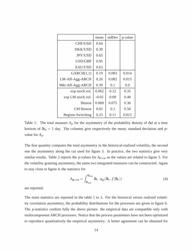
Table 1: The total measureAp for the asymmetry of the probability density of∆σ at a time
horizon ofδtσ = 1 day. The columns give respectively the mean, standard deviation andp-
value forAp.
The first quantity computes the total asymmetry in the historical-realized volatility, the second
one the asymmetry along the cut used for figure 3. In practice,the two statistics give very
similar results. Table 2 reports thep-values forAσ,cut as the values are related to figure 3. For
the volatility graining asymmetry, the same two integratedmeasures can be constructed. Again
to stay close to figure 4, the statistics for
Agr,cut =
Z δtmax
δtmin
δtr agr(δtr , f (δtr)) (4)
are reported.
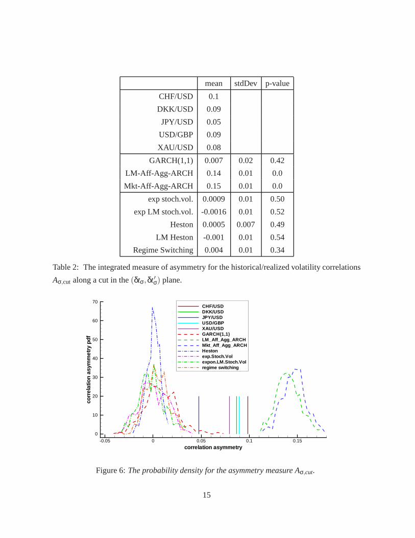
The main statistics are reported in the table 1 to 3. For the historical versus realized volatil-
ity correlation asymmetry, the probability distributionsfor the processes are given in figure 6.
The p-statistics confirm fully the above picture: the empirical data are compatible only with
multicomponent ARCH processes. Notice that the process parameters have not been optimized
to reproduce quantitatively the empirical asymmetry. A better agreement can be obtained for
14
mean stdDev p-value
CHF/USD 0.1
DKK/USD 0.09
JPY/USD 0.05
USD/GBP 0.09
XAU/USD 0.08
GARCH(1,1) 0.007 0.02 0.42
LM-Aff-Agg-ARCH 0.14 0.01 0.0
Mkt-Aff-Agg-ARCH 0.15 0.01 0.0
exp stoch.vol. 0.0009 0.01 0.50
exp LM stoch.vol. -0.0016 0.01 0.52
Heston 0.0005 0.007 0.49
LM Heston -0.001 0.01 0.54
Regime Switching 0.004 0.01 0.34
Table 2: The integrated measure of asymmetry for the historical/realized volatility correlations
Aσ,cut along a cut in the(δtσ,δt ′σ) plane.
correlation asymmetry
corre
latio
nas
ymm
etry
-0.05 0 0.05 0.1 0.15
0
10
20
30
40
50
60
70CHF/USDDKK/USDJPY/USDUSD/GBPXAU/USDGARCH(1,1)LM_Aff_Agg_ARCHMkt_Aff_Agg_ARCHHestonexp.Stoch.Volexpon.LM.Stoch.Volregime switching
Figure 6:The probability density for the asymmetry measure Aσ,cut.
15

mean stdDev p-value
CHF/USD 0.13
DKK/USD 0.1
JPY/USD 0.095
USD/GBP 0.1
XAU/USD 0.08
GARCH(1,1) 0.0008 0.007 0.48
LM-Aff-Agg-ARCH 0.1 0.01 0.0
Mkt-Aff-Agg-ARCH 0.11 0.01 0.0
exp stoch.vol. -0.00007 0.008 0.58
exp LM stoch.vol. -0.0007 0.006 0.54
Heston 0.00007 0.01 0.52
LM Heston 0.0003 0.007 0.59
Regime Switching 0.0002 0.01 0.46
Table 3: The integrated measure of asymmetry for the volatility graining correlationAgr,cut
along a cut in the(δtr ,δt ′r) plane.
16

mean stdDev p-value
CHF/USD -0.21
DKK/USD -0.23
JPY/USD -0.11
USD/GBP -0.08
XAU/USD 0.21
GARCH(1,1) -0.009 0.07 0.54
LM-Aff-Agg-ARCH -0.005 0.07 0.45
Mkt-Aff-Agg-ARCH -0.0009 0.09 0.44
exp stoch.vol. -0.002 0.08 0.42
exp LM stoch.vol. 0.0015 0.08 0.54
Heston -0.002 0.075 0.50
LM Heston 0.002 0.08 0.55
Regime Switching -0.005 0.08 0.59
Table 4: The total measure of the asymmetry of the probability density ofr at a time horizon
of 1 day. The columns give respectively the mean, standard deviation andp-value.
the multicomponent ARCH processes as they contain parameters that control the asymmetry.
This is not possible for other stochastic volatility processes, say for example with respect to
the volatility graining asymmetry: regardless of the parameter values, thep-values stay close to
1/2. Notice also that a simple GARCH(1,1) process can reproduce the asymmetry forap, but
the asymmetry foraσ is too small and the asymmetry foragr is not reproduced at all.
6 Possible origins of time irreversibility
With the help of both the empirical analysis and the process structures, we can speculate on
the origin of the time asymmetry. The systematic study on theprocesses indicates that the
time direction is set by the feed-back loop of the price changes on themselves through the
intermediary of the price volatility, as captured by an ARCHprocess. Moreover, to obtain the
measures of asymmetry with the right magnitudes, multiple time scales must be used in an
17

ARCH structure. This indicates that the interplay between the different time horizons as well
as the feed back loop through the price are enough to create the observed time asymmetry. This
argument emphasises the role of the prices as the only vectorof information between market
participants. By contrast, other “hidden” variables such as an independent stochastic volatility
or other market states are irrelevant with respect to TRI. The picture that emerges is of markets
segmented along the time horizons of the market participants. A more detailed analysis of the
historical versus realized volatilities points in the samedirection, with a cascade from short time
horizons to long horizons [Zumbach and Lynch, 2001, Lynch and Zumbach, 2003].
Another relevant topic with respect to TRI is the connectionbetween news and market be-
haviour. Clearly, financial markets are open systems, driven by various external sources of
information, like exchange of goods, politics, central banks, etc... Even if intuitively clear, the
connection between “news” and financial markets is very difficult to establish from a purely
empirical point. The two fundamental problems are the economic quantification of a “string
of text”, and the discounting by market participants of the “expected” portion of a news. With
respect to TRI, the important question is whether the irreversibly is of external origin (i.e. from
the news) or endogenous (i.e. created by the market participants or the trading rules). As such,
this question is very difficult to investigate empirically,but the present study offers some indi-
rect evidence. In the equations for a process, there is at least one source of randomness, for
example in the return equationr(t) = σ(t) ε(t). Possibly, a process can include several sources
of randomness, like in a stochastic volatility process. Essentially, the random variablesε(t) cap-
ture two different phenomenon: the trades of the market participants (for example through an
order queue), and the influence of the external world (i.e. the news). The canonical hypothesis
for the random processesε is to assume an iid distribution (and independence at a giventime
with the other process variables like price, return, volatility, etc ...). A debatable assumption
is that of time series independence: it is plausible that thenews are serially correlated, as an
important piece of information is likely to be followed by more information. But this is dif-
ficult to establish directly, again because news are given bytexts and not by numbers. In the
investigation of processes, we follow the canonical hypothesis of source of randomness that are
iid. Within this hypothesis, two processes are particularly interesting with respect to TRI. In a
regime switching process, the “state of the world”i(t) exhibits irreversibility, as controlled by
the transition probabilities Pr(i → j), andi(t) has non trivial serial correlations. For this pro-
18

cess, a parallel can be established with the serial correlation of the news. Yet, it is not possible
with a regime switching process to reproduce the observed time asymmetry. On the other hand,
within the framework of iid source of randomness, the multiscale GARCH processes can pro-
vide a quantitatively correct description of the time irreversibility observed in the empirical time
series. Together, both arguments indicate that the time irreversibility is mostly of endogenous
origin, namely created by the interactions between market participants, and not from external
origin.
In a physical system, a common origin of time irreversibility is in friction or dissipation, and
in the increase of entropy. A direct analogy of these quantities in a financial system should be
taken with care. For example, the equivalent of friction canbe thought as the bid-ask spread,
namely the cost for buying, followed by selling directly afterward. However, in a liquid markets,
and particularly in modern electronic trading exchanges, the market orders and limit orders
play a very symmetric role. Using an argument based on the optimal choice of the market
agents between both kind of orders, the authors in [Wyart et al., 2006] show that the profit of a
systematic market making trading strategy should be close to zero. Indirectly, this shows that
the raw cost of trading represents a very small dissipation in the system. In the same direction,
all the simulated processes do not include the cost of transactions, yet all the ARCH processes
are not TRI. Both arguments show that the observed asymmetryin time does not originate in
the bid-ask spread.
Notice that the above discussion on the origin of time irreversibility presents only indirect ar-
guments, as only an investigation of the market microstructure and of the market participant
decision processes can give direct evidence. Yet, such studies are clearly very difficult, and
even more on large decentralised markets as foreign exchanges.
All the measures of asymmetry used so far are even in the returns, and essentially related to
volatilities. The asymmetry in the return distribution is another measure of time asymmetry,
which is odd in the returns. As discussed in the introduction, this symmetry is also related
to the exchange of currencies for the foreign exchange time series. The empirical results for
the return distribution asymmetry are reported in table 4. All the processes have rigorously
symmetric return distributions (because the returns are proportional to the residuals, which
have a symmetric distributions). The results for the processes are in clear agreement with this
19

symmetry, with p-values close to 1/2. Interestingly, the asymmetry for the empirical data is
much larger than for any processes (roughly at 1σ to 2.5 σ from 0). This indicates that the
argument on the exchange of currencies in a FX rate, as given in the introduction, is likely not
correct. Clearly, more extensive investigations are needed to clarify the empirical facts and to
develop processes that can reproduce the observed return asymmetry in the data.
7 Conclusions
To conclude, the systematic study of the time reversal invariance in finance proves to be a very
powerful investigation tool. The empirical time series areclearly not time reversal invariant,
according to three different measures. Although this fact is not obvious at the level of the price
time series, this is not completely surprising as markets are driven by humans, who are clearly
not time reversal invariant. In particular, the market participants remember the past, and this
memory creates an asymmetry in the time direction. More interesting is the fact that different
FX rates show a clear and consistent quantitative pattern. On the modelling side, the ARCH
processes can accommodate the empirical finding, using multiscale processes with increasing
return time horizonsδtr for increasing volatility time horizonsδtσ. The simplest GARCH(1,1)
process can only reproduce some asymmetry, because it contains only one time scale. On
the other hand, all the stochastic volatility and regime switching processes are essentially time
reversal invariant, at odds with the empirical data. This deficiency is related to the structure
of these processes, and is therefore a key shortcoming of this class of models. Eventhough the
various theoretical processes have very different structures, and in particular are not nested, TRI
provides us with a strong selection criterion: a large number of processes cannot reproduce the
stylized facts related to the time irreversibility observed in empirical time series.
8 Acknowledgements
The author thanks Jean-Philippe Bouchaud and Pascal deRougemont for their questions and
discussions on time reversal in finance that initiated this paper.
20

References
[Bollerslev, 1986] Bollerslev, T. (1986). Generalized autoregressive conditional heteroskedas-
ticity. Journal of Econometrics, 31:307–327.
[Breymann et al., 2000] Breymann, W., Zumbach, G., Dacorogna, M. M., and Muller, U. A.
(2000). Dynamical deseasonalization in otc and localized exchange-traded markets. Internal
document WAB.2000-01-31, Olsen & Associates, Seefeldstrasse 233, 8008 Zurich, Switzer-
land.
[Chen et al., 2000] Chen, Y., Chou, R., and Kuan, C. (2000). Testing time irreversibility with-
out moment restrictions.Journal of Econometrics, 95:199–218.
[Dacorogna et al., 2001] Dacorogna, M. M., Gencay, R., Muller, U. A., Olsen, R. B., and
Pictet, O. V. (2001). An Introduction to High-Frequency Finance. Academic Press, San
Diego, CA.
[Dacorogna et al., 1998] Dacorogna, M. M., Muller, U. A., Olsen, R. B., and Pictet, O. V.
(1998). Modelling short-term volatility with GARCH and HARCH models. published in
“Nonlinear Modelling of High Frequency Financial Time Series” edited by Christian Dunis
and Bin Zhou, John Wiley, Chichester, pages 161–176.
[Engle, 1982] Engle, R. F. (1982). Autoregressive conditional heteroskedasticity with estimates
of the variance of U. K. inflation.Econometrica, 50:987–1008.
[Engle and Bollerslev, 1986] Engle, R. F. and Bollerslev, T.(1986). Modelling the persistence
of conditional variances.Econometric Reviews, 5:1–50.
[Fong, 2003] Fong, W. M. (2003). Time irreversibility testsof volume-volatility dynamics for
stock returns.Economics Letters, 81:39–45.
[Lynch and Zumbach, 2003] Lynch, P. and Zumbach, G. (2003). Market heterogeneities and
the causal structure of volatility.Quantitative Finance, 3:320–331.
[Poon, 2005] Poon, S.-H. (2005).A practical Guide to Forecasting Financial Market Volatility.
John Wiley & sons, England.
21

[Ramsey and Rothman, 1988] Ramsey, J. B. and Rothman, P. (1988). Characterization of the
time irreversibility of economic time series: Estimators and test statistics. Working paper
#88-39, C. V. Starr Center for Applied Economics, NYU.
[Ramsey and Rothman, 1996] Ramsey, J. B. and Rothman, P. (1996). Time irreversibility and
business cycle asymmetry.Journal of Money, Credit and Banking, 28(1):1–21.
[Shephard, 2003] Shephard, N. (2003).Stochastic Volatility. Oxford University Press, Oxford.
[Wyart et al., 2006] Wyart, M., Bouchaud, J.-P., Kockelkoren, J., Potters, M., and Vettorazzo,
M. (2006). Relation between bid-ask spread, impact and volatility in double auction markets.
Preprint, arXiv:physics/0603084.
[Zumbach, 2004] Zumbach, G. (2004). Volatility processes and volatility forecast with long
memory.Quantitative Finance, 4:70–86.
[Zumbach and Lynch, 2001] Zumbach, G. and Lynch, P. (2001). Heterogeneous volatility cas-
cade in financial markets.Physica A, 298(3-4):521–529.
22