Embed Size (px)
Citation preview
This is the author’s version of a work that was submitted/accepted for pub-lication in the following source:
Liu, Fawang, Anh, Vo, Turner, Ian, & Zhuang, Pinghui (2003) Time frac-tional advection-dispersion equation. Journal of Applied Mathematics andComputing, 13(1-2), pp. 233-245.
This file was downloaded from: http://eprints.qut.edu.au/22919/
Notice: Changes introduced as a result of publishing processes such ascopy-editing and formatting may not be reflected in this document. For adefinitive version of this work, please refer to the published source:
http://dx.doi.org/10.1007/BF02936089
J. Appl. Math. & Computing Vol. x (200y), No. z, pp.
TIME FRACTIONAL ADVECTION-DISPERSION EQUATION
F.LIU, V.V.ANH, I.TURNER AND P.ZHUANG
Abstract. A time fractional advection-dispersion equation is obtained
from the standard advection-dispersion equation by replacing the first-order derivative in time by a fractional derivative in time of order α(0 <α ≤ 1) . Using variable transformation, Mellin and Laplace transforms,
and properties of H-functions, we derive the complete solution of this timefractional advection-dispersion equation.
AMS Mathematics Subject Classification: 26A33, 49K20, 44A10.Key words and phrases: time fractional advection-dispersion equation,Mellin transform, Laplace transform.
1. Introduction
A space-time fractional partial differential equation, obtained from the stan-dard partial differential equation by replacing the second order space-derivativeby a fractional derivative of order β > 0 and the first order time-derivativeby a fractional derivative of order α > 0 has been recently treated by a num-ber of authors. Wyss (1986) considered the time fractional diffusion equationand the solution was given in closed form in terms of H-functions. Schneiderand Wyss (1989) considered the time fractional diffusion and wave equations.The corresponding Green functions were obtained in closed form for arbitraryspace dimensions in terms of H-functions and their properties were exhibited.Gorenflo, Iskenderov, and Luchko (2000) used the similarity method and theLaplace transform method to obtain the scale-invariant solution of the time-fractional diffusion-wave equation in terms of the Wright function. Benson,Whearcraft and Meerschaert (2000a,b) considered space fractional advection-dispersion equation. They gave an analytical solution featuring the α-stable er-ror function. Liu, Anh and Turner (2002) presented a numerical solution of thespace fractional advection-dispersion equation. Mainardi, Luchko and Pagnini(2001) considered the space-time fractional diffusion equation and provided a
Received , . Revised , .
c⃝ 200x Korean Society for Computational & Applied Mathematics and Korean SIGCAM.
1
2 F. Liu, V. Anh and I. Turner
general representation of the Green functions in the terms of Mellin-Barnes inte-grals in the complex plane. Anh and Leonenko (2000) proposed scaling laws forfractional diffusion-wave equations with singular data. Angulo, Ruiz-Medina,Anh and Grecksch (2000) introduced a fractional heat equation, where the dif-fusion operator is the composition of the Bessel and Riesz potentials. Wyss(2000) considered a fractional Black-Scholes equation and gave a complete solu-tion of this equation. Some partial differential equations of space-time fractionalorder were successfully used for modelling relevant physical processes (Gionaand Roman, 1992; Mainardi, 1994; Hilfer, 1995; Caputo, 1996; Benson, 2000a,b;El-Sayed and Aly, 2002; Basu and Acharya, 2002).
In this paper, we consider the time fractional advection-dispersion equation.This equation is obtained by replacing the time-derivative in the advection dis-persion equation by a generalized derivative of order α with 0 < α ≤ 1. Weconsider
∂αC(x, t)
∂tα= −ν ∂C(x, t)
∂x+D
∂2C(x, t)
∂x2,
x > 0, t > 0, 0 < α ≤ 1 (1)
with the initial condition
C(x, 0) = C0(x), x ≥ 0 (2)
where ν ≥ 0, D > 0 and ∂αC(x,t)∂tα is a fractional derivative.
Properties and more details about the fractional derivatives can be found inSamko, Kilbas and Marichev (1993). Using variable transformation, the timefractional advection-dispersion equation is reduced to a more familiar form. Us-ing Schneider and Wyss’s (1989) and Wyss’s (2000) techniques we derive in thispaper the complete solution of this time fractional advection-dispersion equation(TFADE).
2. The reduced time fractional advection dispersion equation
Eq. (1) can be expressed by the following integral equation (Wyss, 2000;Schneider and Wyss, 1989):
C(x, t) = C(x, 0) +1
Γ(α)
∫ t
0
(t− τ)α−1[−ν ∂C(x, τ)
∂x+D
∂2C(x, τ)
∂x2]dτ
(3)
with n− 1 < α ≤ n ,n = 1. To reduce (3.1) to a more familiar form, let
C(x, t) = u(ξ, t)exp(νξ
2√D), x =
ξ√D
(4)
Time fractional advection-dispersio 3
with the initial condition:
C(x, 0) = C0(x) = u(ξ, 0)exp(− νξ
2√D), ξ > 0. (5)
Let µ2 = ν2
4D , this leads to the equation
u(ξ, t) = u(ξ, 0) +1
Γ(α)
∫ t
0
(t− τ)α−1[∂2u(ξ, τ)
∂ξ2− µ2u(ξ, τ)]dτ (6)
and
u(ξ, 0) = C0(ξ√D)exp(− νξ
2√D). (7)
3. The Green function for the reduced TFADE
According to the properties of the Laplace transform and (49), the Laplacetransform of (6) with respect to t gives for p > 0
u(ξ, p) = p−1u(ξ, 0) + p−α[∂2u(ξ, p)
∂ξ2− µ2u(ξ, p)] (8)
or
∂2u(ξ, p)
∂ξ2− [µ2 + pα]u(ξ, p) = −p−1+αu(ξ, 0). (9)
Letting w2 = µ2 + pα , we have the equation
∂2u(ξ, p)
∂ξ2− w2u(ξ, p) = −p−1+αu(ξ, 0). (10)
According to Schneider and Wyss (1989), Eq. (10) has the solution
u(ξ, p) =
∫ ∞
0
Gαµ(|ξ − y|, p)u(y, 0)dy, (11)
where
Gαµ(r, p) = pα−1κ(r, w) = pα−1κ(r,
√µ2 + pα) (12)
and
κ(r, w) = (r
2πw)
12K 1
2(wr). (13)
A direct transition to the time domain (i.e., inverting the Laplace transform)does not seem to be feasible. This difficulty is circumvented by passing throughthe intermediate step of the Mellin transform (33), connected with the Laplacetransform by (50). Thus, to invert the Laplace transform of Eq. (12) to find
4 F. Liu, V. Anh and I. Turner
Green’s function Gαµ(r, t), we first compute its Mellin transform according to Eq.
(50):
G∗αµ(r, s) =
1
Γ(1− s)
∫ ∞
0
p−sGαµ(r, p)dp (14)
or
G∗αµ(r, s) = (
r
2π)
12
1
Γ(1− s)
∫ ∞
0
p−s+α−1[µ2 + pα]−14K 1
2(r√
µ2 + pα)dp.(15)
Letting q = pα2 , we obtain
G∗αµ(r, s) =
2
α(r
2π)
12
1
Γ(1− s)
∫ ∞
0
q[2−2sα ]−1[µ2 + q2]−
14K 1
2(rõ2 + q2)dq. (16)
Using formula (42) with b = µ, ν = 12 , a = r , we have
G∗αµ(r, s) =
1
α√π(2µ
r)
12 (
2µ
r)−
sαΓ(1− s
α )
Γ(1− s)K s
α− 12(µr). (17)
From the H-function representation (52), we have
H∗1,01,1(−s) = H∗1,0
1,1
(z
∣∣∣∣ (1, 1)(1, 1
α )
)(−s) =
Γ(1− sα )
Γ(1− s). (18)
Let φ(p) = 12exp[−
12µr(p
α+ p−α)] and ϕ(p) = p−α2 φ(p). From the properties
of the Mellin transform and Eqs. (38) and (41), we have
φ∗(s) =1
αK s
α(µr), ϕ∗(s) =
1
αK s
α− 12(µr). (19)
Thus the Mellin transform G∗αµ(r, s) can be written as
G∗αµ(r, s) =
1√π(2µ
r)
12 (
2µ
r)−
sαϕ∗(s)H∗1,0
1,1(−s). (20)
From (38), (40) and (43), we have∫ ∞
0
ϕ((2µ
r)
1αt
z)H1,0
1,1 (z−1)
dz
z
M←→ [(2µ
r)
1α ]−sϕ∗(s)H∗1,0
1,1(−s). (21)
Letting ζ = 1z , we have∫ ∞
0
ϕ((2µ
r)
1αt
z)H1,0
1,1 (z−1)
dz
z=
∫ ∞
0
ϕ((2µ
r)
1α ζt)H1,0
1,1 (ζ)dζ
ζ. (22)
Therefore, the inverse Mellin transform leads to
Gαµ(r, s) =
1√π(2µ
r)
12
∫ ∞
0
ϕ((2µ
r)
1α ζt)H1,0
1,1 (ζ)dζ
ζ(23)
Time fractional advection-dispersio 5
or
Gαµ(r, s) = 1√
π( 2µr )
12
∫∞0
((2µr )1α ζt)−
α2 φ(( 2µr )
1α ζt)H1,0
1,1 (ζ)dζζ
= 12√π√tα
∫∞0
1√ζα
exp[−µ2tαζα − r2
4 t−αζ−α]H1,0
1,1 (ζ)dζζ . (24)
Letting σ = ζα and using the properties (61) and (62) of the H-function, weobtain
Gαµ(r, t)
= 12α
√π√tα
∫∞0
σ− 32 exp[−µ2tασ − r2
4 t−ασ−1]H1,0
1,1
(σ
1α
∣∣∣∣ (1, 1)(1, 1
α )
)dσ
= 12√π√tα
∫∞0
σ− 32 exp[−µ2tασ − r2
4 t−ασ−1]H1,0
1,1
(σ
∣∣∣∣ (1, α)(1, 1)
)dσ
= 12√π√tα
∫∞0
exp[−µ2tασ − r2
4 t−ασ−1]H1,0
1,1
(σ
∣∣∣∣ (1− 3α2 , α)
(− 12 , 1)
)dσ.
(25)
Hence, the inverse Laplace transform of Eq. (11) leads to
u(ξ, t) =
∫ ∞
0
Gαµ(|ξ − y|, t)u(y, 0)dy (26)
4. The complete solution of TFADE
In this section, we find the exact solution of the initial problem (1), (2) withC0(x) = C0. Using the Green function (25) and the initial condition (7), wehave
u(ξ, t) = C0
∫∞0
Gαµ(|ξ − y|, t)exp(−µy)dy
= C0
2√πtα
∫∞0
exp(−µy)dy
×∫∞0
exp(−µ2tασ − 14 (ξ − y)2t−ασ−1)H1,0
1,1
(σ
∣∣∣∣ (1− 3α2 , α)
(−12 , 1)
)dσ
= C0
2√πtα
exp(−µξ)∫∞0
H1,01,1
(σ
∣∣∣∣ (1− 3α2 , α)
(−12 , 1)
)dσ
×∫∞0
exp{−[ ξ−y−2µtασ
2√tασ
]2}dy.
(27)
6 F. Liu, V. Anh and I. Turner
Letting η = 2µtασ−ξ+y
2√tασ
, we get
u(ξ, t) =
C0
2exp(−µξ)
∫ ∞
0
√σH1,0
1,0
(σ
∣∣∣∣ (1− 3α2 , α)
(− 12 , 1)
)dσ
[2√π
∫ ∞
η1
exp{−η2}dη](28)
where η1 = 2µtασ−ξ
2√tασ
.
Using the property (61) of the H-function, we obtain
u(ξ, t) =C0
2exp(−µξ)
∫ ∞
0
H1,01,1
(σ
∣∣∣∣ (1− α, α)(0, 1)
)[erfc(η1)]dσ (29)
where the complementary error function, erfc(x) , is defined as
erfc(x) =2√π
∫ ∞
x
exp(−x2)dx. (30)
Using Eq. (4), we obtain the complete solution for time fractional advectiondispersion equation with 0 < α ≤ 1:
C(x, t) =C0
2
∫ ∞
0
H0,11,1
(σ
∣∣∣∣ (1− α, α)(0, 1)
)[erfc(η1)]dσ. (31)
The function
H1,01,1
(z
∣∣∣∣ (1− α, α)(0, 1)
)is a probability density. From Eqs (59), (60) and (56), we have
H1,01,1
(z
∣∣∣∣ (1− α, α)(0, 1)
)=
∞∑k=0
(−1)k
Γ(1− α− αk)
zk
k!, 0 < α ≤ 1.
(32)
5. Conclusions
The time fractional advection-dispersion equation is obtained from the clas-sical advection-dispersion equation by replacing the first-order time derivativeby a fractional derivative of order α(0 < α ≤ 1).Using variable transformation,the intermediate steps of Mellin and Laplace transforms, we derive the completesolution of this time fractional advection-dispersion equation. Its Green functionincludes a probability density function and a complementary error function.
Acknowledgements
This research has been supported by the ARC SPIRT grant C10024101 andthe National Natural Science Foundation of China 10271098.
Time fractional advection-dispersio 7
Appendix: Preliminaries
For the reader’s convenience we present here certain ideas and the essentialnotions and notations concerning the Mellin and Laplace transforms, which areused in the paper.
Appendix A: The Mellin transform
The Mellin transform of a sufficiently well-behaved function φ onR+ is definedas follows (Samko, Kilbas and Marichev, 1993):
φ∗(s) = M{φ(t); s} =∫ ∞
0
ts−1φ(t)dt (33)
and its inverse is given by the formula
φ∗(t) = M−1{φ(t)∗(s); t} = 1
2πi
∫ γ+i∞
γ−i∞φ∗(s)t−sds, γ = Re(s).
(34)
The Mellin convolution relation is defined as
(h ◦ φ)(t) =∫ ∞
0
h(t
z)φ(z)
dz
z. (35)
The Mellin convolution theorem with respect to (35) takes the form
(h ◦ φ)∗(s) = h∗(s)φ∗(s). (36)
Substituting the expression (36) instead of φ∗(s) in (34) and taking (35) intoaccount we obtain the Parseval relation∫ ∞
0
h(t
z)φ(z)
dz
z=
1
2πi
∫ γ+i∞
γ−i∞h∗(s)φ∗(s)t−sds. (37)
If we denote byM←→ the correspondence between a function and its Mellin
transform, then the following relations of the general types hold:
φ(at)M←→ a−sφ∗(s), a > 0, (38)
taφ(t)M←→ φ∗(s+ a), (39)
φ(tm)M←→ 1
|m|φ∗(
s
m), m = 0, (40)
exp(−ath − bt−h)M←→ 2
h(b
a)
s2hK s
h(2√ab),
Re(a) > 0,Re(b) > 0, h > 0, (41)
(t2 + b2)−12νKν [a(t
2 + b2)12 ]
M←→ a−s2 2
s2−1b
s2−νΓ(
s
2)Kν− s
2(ab),
8 F. Liu, V. Anh and I. Turner
Re(a) > 0,Re(b) > 0,Re(s) > 0, (42)∫ ∞
0
h(t
z)φ(z)
dz
z
M←→ h∗(s)φ∗(s), (43)
where Kν(z) denotes the modified Bessel function of the second kind (Erde’lyi etal., 1954). The Mellin transform formulae of some functions and the propertiesof the Mellin transform can be found in Erde’lyi et al. (1954), Samko, Kilbasand Marichev (1993).
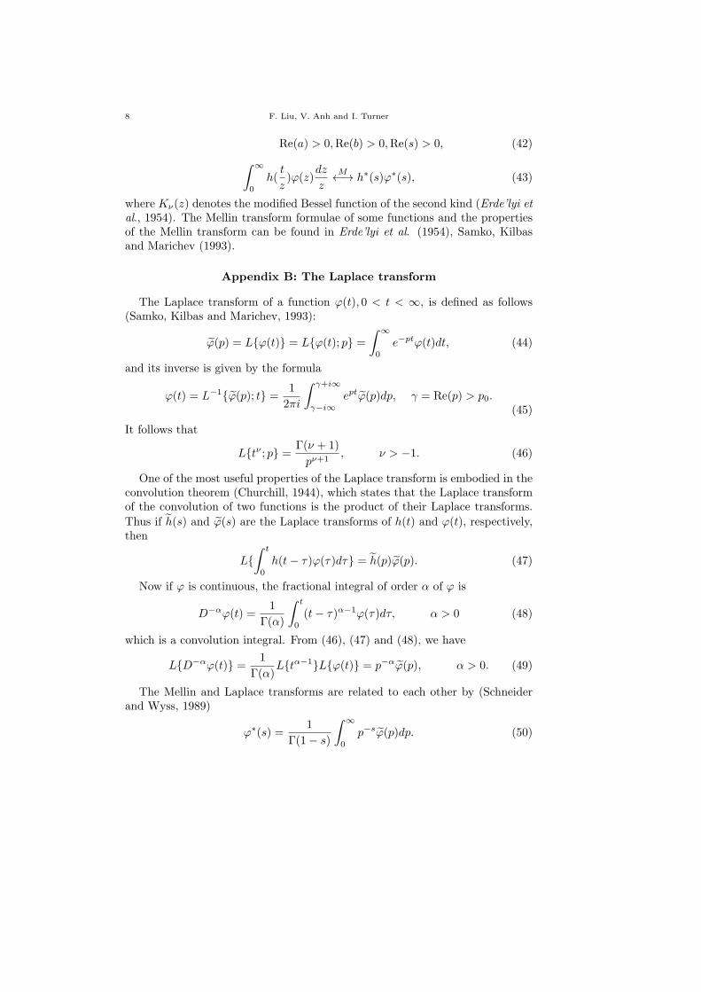
Appendix B: The Laplace transform
The Laplace transform of a function φ(t), 0 < t < ∞, is defined as follows(Samko, Kilbas and Marichev, 1993):
φ(p) = L{φ(t)} = L{φ(t); p} =∫ ∞
0
e−ptφ(t)dt, (44)
and its inverse is given by the formula
φ(t) = L−1{φ(p); t} = 1
2πi
∫ γ+i∞
γ−i∞eptφ(p)dp, γ = Re(p) > p0.
(45)
It follows that
L{tν ; p} = Γ(ν + 1)
pν+1, ν > −1. (46)
One of the most useful properties of the Laplace transform is embodied in theconvolution theorem (Churchill, 1944), which states that the Laplace transformof the convolution of two functions is the product of their Laplace transforms.
Thus if h(s) and φ(s) are the Laplace transforms of h(t) and φ(t), respectively,then
L{∫ t
0
h(t− τ)φ(τ)dτ} = h(p)φ(p). (47)
Now if φ is continuous, the fractional integral of order α of φ is
D−αφ(t) =1
Γ(α)
∫ t
0
(t− τ)α−1φ(τ)dτ, α > 0 (48)
which is a convolution integral. From (46), (47) and (48), we have
L{D−αφ(t)} = 1
Γ(α)L{tα−1}L{φ(t)} = p−αφ(p), α > 0. (49)
The Mellin and Laplace transforms are related to each other by (Schneiderand Wyss, 1989)
φ∗(s) =1
Γ(1− s)
∫ ∞
0
p−sφ(p)dp. (50)
Time fractional advection-dispersio 9
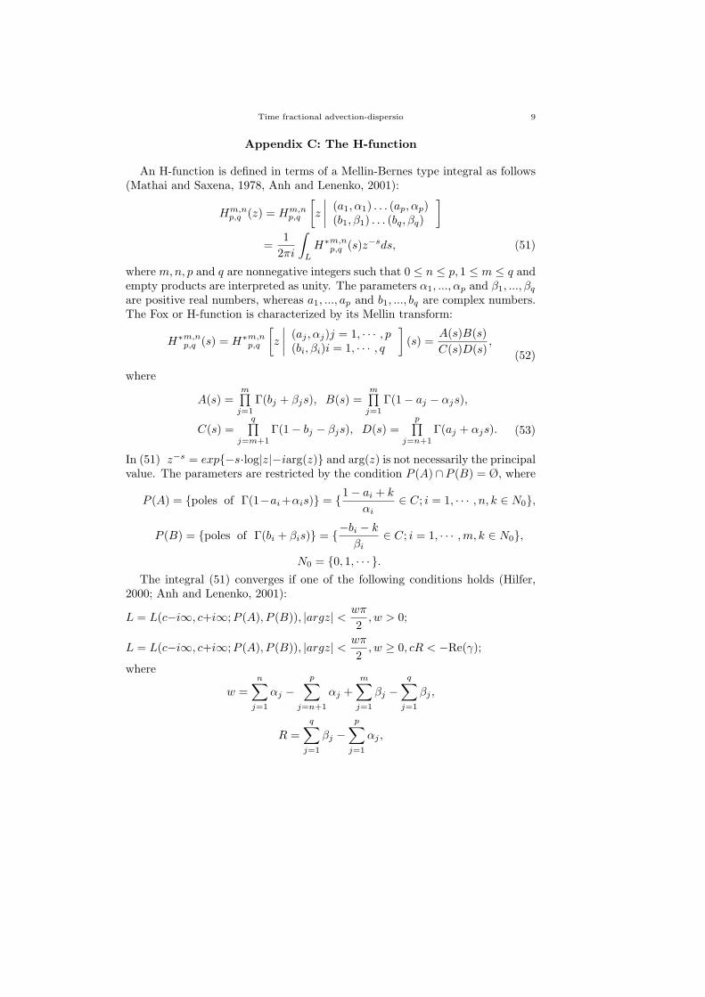
Appendix C: The H-function
An H-function is defined in terms of a Mellin-Bernes type integral as follows(Mathai and Saxena, 1978, Anh and Lenenko, 2001):
Hm,np,q (z) = Hm,n
p,q
[z
∣∣∣∣ (a1, α1) . . . (ap, αp)(b1, β1) . . . (bq, βq)
]=
1
2πi
∫L
H∗m,np,q (s)z−sds, (51)
where m,n, p and q are nonnegative integers such that 0 ≤ n ≤ p, 1 ≤ m ≤ q andempty products are interpreted as unity. The parameters α1, ..., αp and β1, ..., βq
are positive real numbers, whereas a1, ..., ap and b1, ..., bq are complex numbers.The Fox or H-function is characterized by its Mellin transform:
H∗m,np,q (s) = H∗m,n
p,q
[z
∣∣∣∣ (aj , αj)j = 1, · · · , p(bi, βi)i = 1, · · · , q
](s) =
A(s)B(s)
C(s)D(s),
(52)
where
A(s) =m∏j=1
Γ(bj + βjs), B(s) =m∏j=1
Γ(1− aj − αjs),
C(s) =q∏
j=m+1
Γ(1− bj − βjs), D(s) =p∏
j=n+1
Γ(aj + αjs). (53)
In (51) z−s = exp{−s·log|z|−iarg(z)} and arg(z) is not necessarily the principalvalue. The parameters are restricted by the condition P (A)∩P (B) = Ø, where
P (A) = {poles of Γ(1−ai+αis)} = {1− ai + k
αi∈ C; i = 1, · · · , n, k ∈ N0},
P (B) = {poles of Γ(bi + βis)} = {−bi − k
βi∈ C; i = 1, · · · ,m, k ∈ N0},
N0 = {0, 1, · · · }.The integral (51) converges if one of the following conditions holds (Hilfer,
2000; Anh and Lenenko, 2001):
L = L(c−i∞, c+i∞;P (A), P (B)), |argz| < wπ
2, w > 0;
L = L(c−i∞, c+i∞;P (A), P (B)), |argz| < wπ
2, w ≥ 0, cR < −Re(γ);
where
w =
n∑j=1
αj −p∑
j=n+1
αj +
m∑j=1
βj −q∑
j=1
βj ,
R =
q∑j=1
βj −p∑
j=1
αj ,
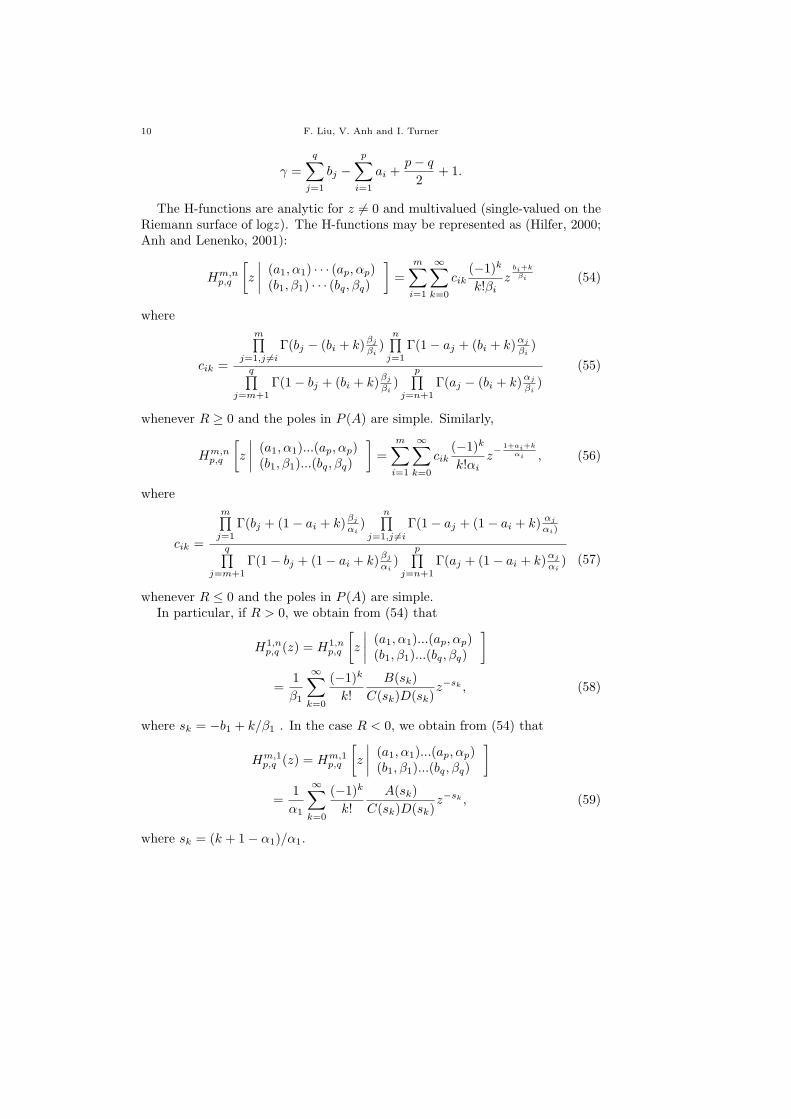
10 F. Liu, V. Anh and I. Turner
γ =
q∑j=1
bj −p∑
i=1
ai +p− q
2+ 1.
The H-functions are analytic for z = 0 and multivalued (single-valued on theRiemann surface of logz). The H-functions may be represented as (Hilfer, 2000;Anh and Lenenko, 2001):
Hm,np,q
[z
∣∣∣∣ (a1, α1) · · · (ap, αp)(b1, β1) · · · (bq, βq)
]=
m∑i=1
∞∑k=0
cik(−1)k
k!βiz
bi+k
βi (54)
where
cik =
m∏j=1,j =i
Γ(bj − (bi + k)βj
βi)
n∏j=1
Γ(1− aj + (bi + k)αj
βi)
q∏j=m+1
Γ(1− bj + (bi + k)βj
βi)
p∏j=n+1
Γ(aj − (bi + k)αj
βi)
(55)
whenever R ≥ 0 and the poles in P (A) are simple. Similarly,
Hm,np,q
[z
∣∣∣∣ (a1, α1)...(ap, αp)(b1, β1)...(bq, βq)
]=
m∑i=1
∞∑k=0
cik(−1)k
k!αiz− 1+ai+k
αi , (56)
where
cik =
m∏j=1
Γ(bj + (1− ai + k)βj
αi)
n∏j=1,j =i
Γ(1− aj + (1− ai + k)αj
αi)
q∏j=m+1
Γ(1− bj + (1− ai + k)βj
αi)
p∏j=n+1
Γ(aj + (1− ai + k)αj
αi) (57)
whenever R ≤ 0 and the poles in P (A) are simple.In particular, if R > 0, we obtain from (54) that
H1,np,q (z) = H1,n
p,q
[z
∣∣∣∣ (a1, α1)...(ap, αp)(b1, β1)...(bq, βq)
]=
1
β1
∞∑k=0
(−1)k
k!
B(sk)
C(sk)D(sk)z−sk , (58)
where sk = −b1 + k/β1 . In the case R < 0, we obtain from (54) that
Hm,1p,q (z) = Hm,1
p,q
[z
∣∣∣∣ (a1, α1)...(ap, αp)(b1, β1)...(bq, βq)
]=
1
α1
∞∑k=0
(−1)k
k!
A(sk)
C(sk)D(sk)z−sk , (59)
where sk = (k + 1− α1)/α1.
Time fractional advection-dispersio 11
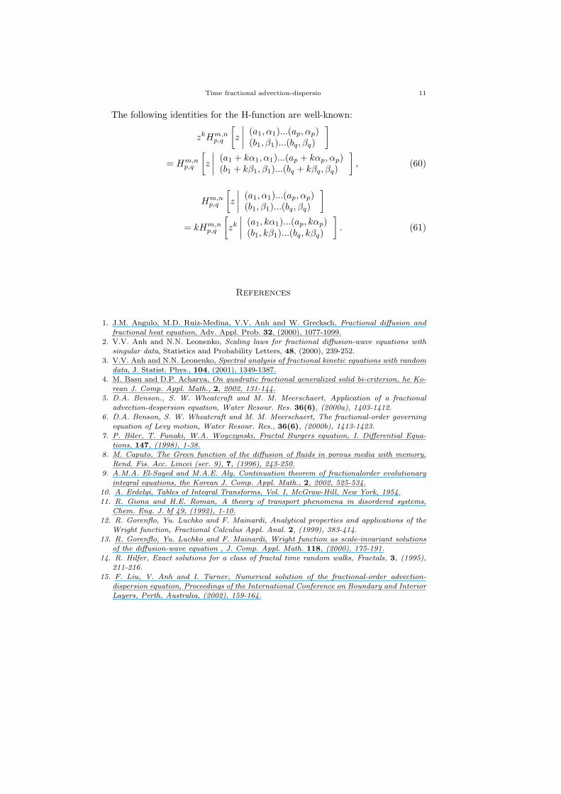
The following identities for the H-function are well-known:
zkHm,np,q
[z
∣∣∣∣ (a1, α1)...(ap, αp)(b1, β1)...(bq, βq)
]= Hm,n
p,q
[z
∣∣∣∣ (a1 + kα1, α1)...(ap + kαp, αp)(b1 + kβ1, β1)...(bq + kβq, βq)
], (60)
Hm,np,q
[z
∣∣∣∣ (a1, α1)...(ap, αp)(b1, β1)...(bq, βq)
]= kHm,n
p,q
[zk
∣∣∣∣ (a1, kα1)...(ap, kαp)(b1, kβ1)...(bq, kβq)
]. (61)
References
1. J.M. Angulo, M.D. Ruiz-Medina, V.V. Anh and W. Grecksch, Fractional diffusion and
fractional heat equation, Adv. Appl. Prob. 32, (2000), 1077-1099.2. V.V. Anh and N.N. Leonenko, Scaling laws for fractional diffusion-wave equations with
singular data, Statistics and Probability Letters, 48, (2000), 239-252.3. V.V. Anh and N.N. Leonenko, Spectral analysis of fractional kinetic equations with random
data, J. Statist. Phys., 104, (2001), 1349-1387.4. M. Basu and D.P. Acharya, On quadratic fractional generalized solid bi-criterion, he Ko-
rean J. Comp. Appl. Math., 2, 2002, 131-144.5. D.A. Benson., S. W. Wheatcraft and M. M. Meerschaert, Application of a fractional
advection-despersion equation, Water Resour. Res. 36(6), (2000a), 1403-1412.6. D.A. Benson, S. W. Wheatcraft and M. M. Meerschaert, The fractional-order governing
equation of Levy motion, Water Resour. Res., 36(6), (2000b), 1413-1423.
7. P. Biler, T. Funaki, W.A. Woyczynski, Fractal Burgers equation, I. Differential Equa-tions, 147, (1998), 1-38.
8. M. Caputo, The Green function of the diffusion of fluids in porous media with memory,Rend. Fis. Acc. Lincei (ser. 9), 7, (1996), 243-250.
9. A.M.A. El-Sayed and M.A.E. Aly, Continuation theorem of fractionalorder evolutionaryintegral equations, the Korean J. Comp. Appl. Math., 2, 2002, 525-534.
10. A. Erdelyi, Tables of Integral Transforms, Vol. I, McGraw-Hill, New York, 1954.11. R. Giona and H.E. Roman, A theory of transport phenomena in disordered systems,
Chem. Eng. J. bf 49, (1992), 1-10.12. R. Gorenflo, Yu. Luchko and F. Mainardi, Analytical properties and applications of the
Wright function, Fractional Calculus Appl. Anal. 2, (1999), 383-414.13. R. Gorenflo, Yu. Luchko and F. Mainardi, Wright function as scale-invariant solutions
of the diffusion-wave equation , J. Comp. Appl. Math. 118, (2000), 175-191.14. R. Hilfer, Exact solutions for a class of fractal time random walks, Fractals, 3, (1995),
211-216.15. F. Liu, V. Anh and I. Turner, Numerical solution of the fractional-order advection-
dispersion equation, Proceedings of the International Conference on Boundary and InteriorLayers, Perth, Australia, (2002), 159-164.
12 F. Liu, V. Anh and I. Turner
16. F. Mainardi, On the initial value problem for the fractional diffusion-wave equation, in :
S. Rionero, T. Ruggeri (Eds.) , Waves and Stability in Continuous Media, World Scien-tific, Singapore, (1994), 246-251.
17. F. Mainardi, Fractional diffusive waves in viscoelastic solids in: J.L. Wagner and F.R.Norwood (Eds.), IUTAM Symposium - Nonlinear Waves in Solids, ASME/AMR, Fairfield
NJ, (1995), 93-97.18. F. Mainardi, Yu. Luchko and G. Pagnini, The fundamental solution of the space-time
fractional diffusion equation, Fractional Calculus Appl. Anal., 4, (2001).19. K.S. Miller and B. Ross, An Introduction to the Fractional Calculus and Fractional Dif-
ferential Equations, John Wiley, New York, 1993.20. K.B. Oldham and J. Spanier, The Fractional Calculus, Academic Press, 1974.21. I. Podlubny, Fractional Differential Equations, Academic Press, 1999.22. A. Saichev and G. Zaslavsky, Fractional kinetic equations: solutions and applications,
Chaos, 7, (1997), 753-764.23. S.G. Samko, A. A. Kilbas, and O. I. Marichev, Fractional Integrals and Derivatives:
Theory and Applications, Gordon and Breach, Newark, N J, 1993.24. W.R. Schneider and W. Wyss, Fractional diffusion and wave equations, J. Math. Phys.
30, (1989), 134-144.25. W. Wyss, The fractional diffusion equation, J. Math. Phys., 27, (1986), 2782-2785.26. W. Wyss, The fractional Black-Scholes equation, Fractional Calculus Appl. Anal. 3,
(2000), 51-61.
Fawang Liu received his MSc from Fuzhou University in 1982 and PhD from Trinity Col-lege, Dublin, in 1991. Since graduation, he has been working in computational and applied
mathematics at Fuzhou University, Trinity College Dublin and University College Dublin,University of Queensland, Queensland University of Technology and Xiamen University.Now he is a Professor at Xiamen University. His research interest is numerical analysisand techniques for solving a wide variety of problems in applicable mathematics, including
semiconductor device equations, microwave heating problems, gas-solid reactions, singularperturbation problem, saltwater intrusion into aquifer systems and fractional differentialequations.
(1) Department of Mathematics, Xiamen University, Xiamen 361005, China (2) Schoolof Mathematical Sciences, Queensland University of Technology, Qld. 4001, Australia.
e-mail: [email protected]
Vo Anh received his PhD degree from the University of Tasmania, Australia, in 1978. He
has been with Queensland University of Technology since 1984. His research interests in-clude stochastic processes and random fields, fractional diffusion, environmental modellingfinancial modelling.
School of Mathematical Sciences, Queensland University of Technology, Qld. 4001, Aus-tralia.
e-mail: [email protected]
Ian Turner is a senior lecturer at the School of Mathematical Science, QUT. He has
extensive experience in the solution of systems of non-linear partial differential equationsusing the finite volume discretisation process and has written numerous journal publica-tions in the field. He has been awarded outstanding paper awards from two internationaljournals for his modelling work, with the most significantcontribution being the use of
mathematical models for furthering the understanding of how microwaves interact withlossy materials during heating and drying processes. He also has considerable expertise in
Time fractional advection-dispersio 13
solving large sparse non-linear and linear systems via preconditioned Krylov based meth-
ods.
School of Mathematical Sciences, Queensland University of Technology, Qld. 4001, Aus-tralia.
e-mail: [email protected]
Zhuang Pinghui received his BSc and MSc from Fuzhou University in 1982 and 1988respectively. Since graduation, he has been working in computational and applied mathe-matics at Xiamen University. Now he is an associate professor. His research interest is
numerical analysis and techniques for solving singular perturbation problem and fractionaldifferential equations, numerical simulation for saltwater intrusion into aquifer systemsand computing.
Department of Mathematics, Xiamen University, Xiamen 361005, China.e-mail: [email protected]


