Fractional-Order Viscoelasticity (FOV): Constitutive Development Using the Fractional Calculus: First Annual Report

NASA/TM--2002-211914

Fractional-Order Viscoelasticity (FOV):

Constitutive Development Using the

Fractional Calculus: First Annual Report

Alan Freed

Glenn Research Center, Cleveland, Ohio

Kai Diethehn

Technisch.e Un.:i.versit_it Braunschweig, Braunschweig, Germany

Yury Luchko

Europe University Via drina, Frankfurt, Germany

December 2002

The NASA STI Program Office... in Profile

Since its founding, NASA has been dedicated to

the advancement of aeronautics and spacescience. Tile NASA Scientific and Technical

Information (STI) Program Office plays a key part

in helping NASA maintain this important role.

Tile NASA STI Program Office is operated by

Langley Research Center, the Lead Center forNASA's scientific and technical information. The

NASA STI Program Office provides access to the

NASA STI Database, the largest collection of

aeronautical and space science STI in file world.

The Program Office is also NASA's institutional

medlanism for disseminating the results of its

researd3 and development acti vities. These results

are published by NASA in the NASA STI Report

Series, which includes the following report types:

TECHNICAL PUBHCATION. Reports of

completed :research or a major significant

phase of research that present the results of

NASA programs and include extensive data

or theoretical analysis. Includes compilations

of significant scientific and technical data and

information deemed to be of continuing

reference value. NASA's counterpart of peer-

reviewed formal professional papers but

has less stringent limitations on manuscript

lengfl3 and extent of graphic presentations.

TECHNICAL MEMORANDUM. Scientific

and tedmical findings that are pre, liminary or

of specialized interest, e.g., quick release

reports, working papers, and bibliographiesthat contain minimal annotation. Does not

contain extensive analysis.

CONTRACTOR REPORT. Scientific and

technical findings by NASA-sponsored

contractors and grantees.

CONFERENCE PUBLICATION. Collected

papers from scientific and technical

conferences, symposia, seminars, or other

meetings sponsored or cosponsored byNASA.

SPECIAL PUBLICATION. Scientific,

technical, or historical information from

NASA programs, projects, and missions,

often concerned with subjects having

substantial public interest.

TECHNICAL TRANSLATION. English-

language translations of foreign scientific

and technical material pertinent to NASA'smission.

Specialized services that complement the STI

Program Office's diverse offerings include

creating custom thesauri, building customized

databases, organizing and publishing research

results.., even providing videos.

For more information about the NASA STI

Program Office, see the following:

® Access the NASASTI Program Home Page

at http:lhuww.sti.nasa.gov

® E-mail your question via the Intemet to

[email protected]

* Fax your question to the NASA Access

Help Desk at 301-621-0134

* Telephone the NASA Access Help Desk at301-621-0390

Write to:

NASA Access Help Desk

NASA Center for AeroSpace Information7121 Standard Drive

Hanover, MD 21076

NASA/TM--2002-211914

Fractional-Order Viscoelasticity (FOV):

Constitutive Development Using the


Alan Freed

Glenn Research Ce:nter, CleveI.and, Ohio

Kai Diethehn

Technisch.e Un.iversit_it Braunschweig, Braunschweig, Germany

Yury Luchko

Europe University Via drina, Frankfurt, Germany

National Aeronautics and

Spa ce Administration

Glelm Research Center

December 2002

Acknowledgments

Alan Freed would like to thank Prof. Ronald Bagley, University of Texas-San Antonio (then Col. Bagley, USAF), for

encouraging him to study the fractional calculus and to use FOV in his research on polymers and soft tissues. Thiswork was supported in part by the U.S. Army Medical Research and Material Command to the Cleveland Clinic

Foundation with NASA Glenn Research Center being a subcontractor through Space Act Agreement SAA 3---445.Numerous discussions with the PI, Dr. Ivan Vesle?, and two of his research associates, Dr. Evelyn Carew and

Dr. Todd Doehring, are gratefully acknowledged. Additional support was supplied by the UltraSafe Project at theNASA Glenn Research Center. Alan Freed also gratefully acknowledges the encouragement and support of: project

manager, Mr. Dale Hopkins, and supervisor, Dr. Michael Meador, at the NASA Glenn Research Center.

This report contains preliminary

findings, subject to revision asanalysis proceeds.

The Aerospace Propulsion and Power Program atNASA Glenn Research Center sponsored this work.

NASA Center for Aerospace Information71121Standard Drive

Hanover, MD 211076

Available from

National Technical Information Service

5285 Port Royal RoadSpringfield, VA 22100

Available electronically at http://gltrs.grcnasa.gov

Contents

1 Fractional Calculus 1

1.1 Riemann-Liouville Fractional Integral .................. 1

1.2 Caputo-Type Fractional Derivative ................... 2

1.2.1 Integral Expressions ....................... 3

1.3 Caputo-Type FDE's ........................... 4

1.4 Numerical Approximations ........................ 5

1.4.1 Caputo-type Fractional Derivatives ............... 5

1.4.2 Riemann-Liouville Fractional Integrals ............. 8

1.4.3 Caputo-Type FDE's ....................... l0

1.5 Mittag-Leffier Function .......................... 13

1.5.1 Analytical Properties ....................... 13

1.5.2 Numerical Algorithms ...................... 15

2 1D FOV 17

2.1 Material Functions ............................ 19

2.1.1 Static Experiments ........................ 20

2.1.2 Dynamic Experiments ...................... 24

3 Continuum Mechanics 29

3.1 Metric Fields ............................... 29

3.1.1 Dual ................................ 30

3.1.2 Rates ............................... 31

3.2 Strain Fields ................................ 32

3.2.1 Covariant ............................. 32

3.2.2 Contravariant ........................... 33

3.2.3 Dilatation ............................. 34

3.3 Stress Fields ................................ 35

3.3.1 Rates ............................... 36

4 Field Transfer 37

4.1 Kinematics ................................ 37

4.2 Deformation Fields ............................ 39

4.2.1 Duals ............................... 39

4.2.2 Rates ............................... 40

4.3 Field Transfer of Fractional Operators ................. 44

NASA/T_2002-211914 iii

4.3.1 Derivatives ............................ 45

4.3.2 Integrals .............................. 47

4.4 Strain Fields ................................ 48

4.4.1 Covariant-Like .......................... 49

4.4.2 Contravariant-Like ........................ 50

4.4.3 Dilational ............................. 51

4.5 Stress Fields ................................ 52

4.5.1 Conservation Laws ........................ 52

4.5.2 Rates ............................... 53

5 Constitutive Theories 55

5.1 Integrity Bases .............................. 55

5.2 Elasticity ................................. 56

5.3 Viscoelasticity ............................... 57

5.4 Tangent Operator ............................. 59

5.4.1 Stability .............................. 60

5.5 Isotropic Elasticity ............................ 61

5.5.1 Field transfer ........................... 65

5.6 Isotropic Viscoelasticity ......................... 68

5.6.1 Field transfer ........................... 69

5.7 Transversely Isotropic Elasticity ..................... 70

5.7.1 Field transfer ........................... 72

5.8 Transversely Isotropic Viscoelasticity .................. 75

5.8.1 Field transfer ........................... 76

6 Finite-Strain Experiments 79

6.1 Shear-Free Extensions .......................... 79

6.1.1 Kinematics ............................ 79

6.1.2 Deformation Fields ........................ 81

6.1.3 Strain Fields ............................ 82

6.1.4 Stress Fields ............................ 84

6.1.5 Special Cases ........................... 85

6.2 Simple Shear ............................... 86

6.2.1 Kinematics ............................ 86

6.2.2 Deformation Fields ........................ 88

6.2.3 Strain Fields ............................ 89

6.2.4 Stress Fields ............................ 92

7 Bulk Material Models 93

7.1 Elastic Response ............................. 93

7.1.1 Theory for pressure ........................ 96

7.2 Viscoelastic Response ........................... 97

7.2.1 Voigt solid ............................. 98

7.2.2 Kelvin solid ............................ 98

7.2.3 Fractional-order models ..................... 99

NASA/T_2002-211914 iv

7.3 Bridgman'sExperiment ......................... 73

A Table of Caputo Derivatives 105

B Automatic Integration 107B.1 The FundamentalStrategy ........................ 107B.2 Approximation of the Integral ...................... 108B.3 Approximation of Error Estiamtes.................... 108

C Table of Pad_ Approximates for Mittag-Leffler Function 111

NASA/T_2002-211914 v

Nomenclature

Numbers

N

N0R

C

natural numbers, N := {1, 2, 3,...}

counting numbers, No := {0, 1, 2,...}

real numbers

positive real numbers, R+ := {a E R • a > 0}

complex numbers, C := {x + i y • x, y E 11(;i := v/-_}

Functions

n

E.(x)E.,,(x)1Fl(a; b; x)

2Fl(a, b; c; x)

U(x - zo)5(x)

r(x)

set of all continuous n-differentiable functions

Mittag-Leffler function in one parameter, (_

Mittag-Lemer function in two parameters, a &: f_

Kummer confluent hypergeometric function

Gauss hypergeometric function

unit step function

Dirac delta distribution (the generalized function usually characterized

by the property that f_oo 5(x).f(x)dx := 5If] := f(O) whenever f is

continuous at 0)

Euler's continuous gamma function

digamma function

Differential and Integral Operators

n

D o

D."J_

J_

differential operator, n E N

Riemann-Liouville fractional differential operator, c_ E ]i¢+

Caputo fractional differential operator, c_ E R+

Cauchy n-fold integral operator, n E N

Riemann-Liouville fractional integral operator, (_ E

Scalar Fields

Ai

dA

dC

dH

dS

surface area whose normal points in the ith coordinate direction

differential element for area-of-surface

reference distance separating neighboring planes

differential element for height-of-separation between planes

differential element for distance-of-separation between points

NASA/T_2002-211914 vii

dV

C

f

fi

G

G' & G"

J

g

_o

P

P

8

S

T

Vs

W

OL, Oq

7

6

C

A

#

P, Pi

Q

O"

oi

differential element for volume-of-mass

dilatation

force in 1D

force in the ith coordinate direction

force in the ith coordinate direction acting on a surface whose unit

normal is in the jth coordinate direction

viscoelastic (or relaxation) modulus

viscoelastic storage and loss (dynamic) moduli

ith relaxation function

n th invariant of an integrity basis

viscoelastic compliance

current length of gauge section

gauge length

ith memory function

hydrostatic pressure

Lagrange multiplier forcing an isotropic constraint

Laplace transform variable

magnitude of shear

time

absolute temperature

speed of sound

work

potential function representing work

fractal order of evolution

fractal order of evolution in bulk response

viscoelastic material constant

engineering shear strain

dilatation, classic definition

dilatation, Hencky's definition

strain in I-D

viscosity

bulk modulus

principal stretch ratio

stretch along fiber direction

ith principal stretch ratio

elastic shear modulus

characteristic retardation time

characteristic bulk retardation time

mass density

stress in I-D

ith principal stress

reaction stress

NASA/T_2002-211914 viii

7"

T, T{

91

92

co

shear stress

characteristic relaxation time

characteristic bulk relaxation time

first normal-stress difference

second normal-stress difference

angular frequency (rad/sec)

Outer Products

a®b

A®B_

A_Nb

vector outer product with components aibj where i, j = 1, 2, 3

tensor outer product with components AijBkt where i, j, k, _, = 1, 2, 3

1 (AikBjl + AffBjk)symmetric tensor outer product with componentswhere i, j, k, e = 1, 2, 3

Body

B

q3

manifold, _ E N 3

coordinate system

particle (a material point)

coordinates, { = (_1, _2, _3)

Body Vector and Tensor Fields

A

d_ & d_

dq5

c_0

6

9,-1

E

¢

r/

0

A

v

7r

71"

FI

fourth-order, contravariant, tangent operator

coordinate differences between neighboring particles

contact force acting on differential area

contravariant unit vector in preferred material direction

contravariant areal strain tensor

mixed idem tensor

covariant metric tensor

contravariant metric tensor

covariant strain tensor (strain between material points)

contravariant strain tensor (strain between material planes)

arbitrary contravariant tensor

tensor of arbitrary weight, kind and rank

mixed stretch tensor

arbitrary covariant tensor

covariant unit normal vector

contravariant stress tensor

contravariant deviatoric stress tensor

contravariant extra-stress tensor

Body Tensor Rates

NASA/TM--2002-211914 ix

D

D.J_

partial derivative

Caputo fractional derivative

Riemann-Liouville fractional integral

Field Transfer

t

' to

Eulerian transfer of field: body into Cartesian space

Lagrangian transfer of field: body into Cartesian space

Cartesian Space

S

C

Xo

X

X

X

I

manifold, S E N 3

(rectangular) Cartesian coordinate system

place containing particle _3 in initial state to

reference (Lagrangian) position vector to 3¢0 with coordinates X =

(X1, X2, Xa) in C

place containing particle _ in current state t

current (Eulerian) position vector to :_ with coordinates x = (xl, x2, xa)in C

unit tensor

Kinematic Fields

a

v

F

L

R

acceleration vector

velocity vector

deformation gradient tensor

velocity gradient tensor

orthogonal rotation tensor

Eulerian Vector and Tensor Fields

a

fn

A

A (n)

B

C

C a

C e

C ea

C"

unit vector in preferred material direction

coordinate differences between neighboring places

body-force vector

unit-normal vector

Almansi strain tensor (strain between material points)

generalized anisotropic strain tensor of order n

Finger deformation tensor

fourth-order tangent operator

anisotropic part of elastic tangent operator

isotropic elastic part of viscoelastic tangent operator

anisotropic elastic part of viscoelastic tangent operator

isotropic viscous part of viscoelastic tangent operator

NASA/T_2002-211914 x

m

E (")

G

G

J

M

M

T

V

Z

anisotropic viscous part of viscoelastic tangent operator

generalized strain tensor of order n

arbitrary contravariant-like tensor

fourth-order relaxation modulus

arbitrary tensor

arbitrary covariant-like tensor

fourth-order memory function

Cauchy stress tensor

deviatoric Cauchy stress tensor

left stretch tensor

Signorini strain tensor (strain between material planes)

spatial-gradient operator, 0/0x

Eulerian Tensor Rates

a_0

D, O/Ot

D

c,rD

D

}W

M

lOtMW

unit vector in preferred material direction

partial derivative

material derivative

rate-of-deformation tensor

upper-fractal rate-of-deformation tensor of order a

lower-fractal rate-of-deformation tensor of order a

upper-convected (Oldroyd) derivative of a contravariant-like tensor G

upper-fractal derivative of order a of a contravariant-like tensor _G

upper-fractal integral of order a of a contravariant-like tensor G

corotational (Zaremba-Jaumann) derivative of an arbitrary tensor Y_

lower-convected (Oldroyd) derivative of a covariant-like tensor M

lower-fractal derivative of order c_ of a covariant-like tensor M

lower-fractal integral of order a of a covariant-like tensor M

vorticity tensor

Lagrangian Vector and Tensor Fields

A

dX & dX

N

C

C

E

H

N

coordinate differences between neighboring places

unit-normal vector

Green deformation tensor

fourth-order tangent operator

Green strain tensor (strain between material points)

arbitrary contravariant-like tensor

arbitrary covariant-like tensor

NASA/T_2002-211914 xi

P

p*

U

Y

Div

second Piola-Kirchhoff stress tensor

deviatoric part of second Piola-Kirchhoff stress tensor

Lagrangian stress tensor

right stretch tensor

Lagrangian strain tensor (strain between material planes)

spatial-gradient operator, O/OX

Lagrangian Tensor Rates

D

J_

partial derivative

Caputo fractional derivative

Riemann-Liouville fractional integral

NASA/T_2002-211914 xii

Preface

This is the first annual report to the U.S. Army Medical Research and Material

Command for the three year project "Advanced Soft Tissue Modeling for Telemedicine

and Surgical Simulation" supported by grant No. DAMDI7-01-1-0673 to The Cleve-

land Clinic Foundation, to which the NASA Glenn Research Center is a subcontractor

through Space Act Agreement SAA 3-445.

The objective of this report is to extend popular one-dimensional (ID) fractional-

order viscoelastic (FOV) material models into their three-dimensional (3D) equiva-

lents for finitely deforming continua, and to provide numerical algorithms for their

solution. The present report is organized into seven chapters and three appendices.

The first chapter serves as an introduction to the fractional calculus. Algorithms

for computing fractional derivatives, fractional integrals, fractional-order differential

equations (FDE's), and the Mittag-Lemer function (which apprears in analytic solu-

tions of FDE's) are provided.

One of the oldest applications of the fractional calculus is viscoelasticity. Chapter

two presents an overview of ID FOV. Definitions for the standard FOV fluid and

the standard FOV solid are put forth along with formulae that are useful in their

characterization, assuming infinitesimal strains and rotations.

The third chapter provides an overview of continuum mechanics using body (i.e.,

convected) tensor fields. Three strain fields are introduced that are measures of

strain based on changes in: length of line, separation of non-intersecting surfaces,

and volmne of mass. Introduced here for the first time are fractal rates of arbitrary

tensor fields. Body fields are useful when deriving contitutive equations.

In the fourth chapter, the body fields defined in the previous chapter are mapped

into objective, Cartesian, space fields. A useful by-product of field transfer is that

those spatial fields created by field transfer are frame invariant. Spatial fields are

useful when solving boundary-value problems.

The fifth chapter derives isotropic and transverse-isotropic theories for elastic and

viscoelastic materials by applying a work potential to an integrity basis. Both com-

pressible and incompressible materials are considered. These theories are derived

in the body and then transferred into Cartesian space in both the Eulerian and La-

grangian frames. The tangent modulus is derived for the general theoretical structuresof elastic and viscoelastic solids.

A suite of homogeneous experiments used to characterize material models is pre-

sented in the sixth chapter. The suite includes the homogeneous deformations of:

shear-free extension (e.g., uniaxial elongation, biaxial extension, pure shear, and di-

lational compression) and simple shear. The deformation, stress and strain fields

NASA/T_2002-211914 xiii

definedin the prior chapter,alongwith their variousrates,areall quantifiedfor thissuiteof experiments.

Chaptersseventhrough nine provideelastic and viscoelasticconstitutivemodelsappropriatefor 3D analysis. Chapter sevenprovidesmaterial modelsfor bulk re-sponse.Chaptereight will introducematerial modelsfor isotropic elastomers,whilechapterninewill introducematerial modelsfor soft biologicaltissues,which aregen-erally transverseisotropic;they will becompletedfor the secondannualreport. Bothclassicalandfractional-orderviscoelasticmodelsarepresented.Includedaresolutionsfor the characterizationexperimentsof chaptersix.

Therearethreeappendices.The first appendixtabulatesCaputofractionalderiva-tives for a few of the more commonmathematicalfunctions. The secondappendixoutlinesanautomaticprocedurefor numericalintegrationthat is requiredby thealgo-rithm whichcomputesthe Mittag-Leffier function. And the third appendixprovidesan efficientschemefor approximatinga specificform of the Mittag-Lemer functionthat arisesin FOV.

NASA/T_2002-211914 xiv

Chapter 1

Fractional Calculus:

numerical methods

1.1 Riemann-Liouville Fractional Integral

In the classical calculus of Newton and Leibniz, Cauchy reduced the calculation of an

n-fold integration of the function y(x) into a single convolution integral possessing

an Abel (power law) kernel,

Jny(x) := "'" y(x0) dxo.., dx,_-2 dx,_-i

1 _ 1 (1.1)

-(n-1)!f, noN, xe ,

where J'_ is the n-fold integral operator with d_y(x) = y(x), N is the set of positive

integers, and N+ is the set of positive reals. Liouville and Riemann* analytically

continued Cauchy's result by replacing the discrete factorial (n - 1)! with Euler's

continuous gamma function F(n), noting that (n-1)Y = F(n), thereby producing [67,

Eqn. AI

JaY(X) := (x - x') 1-a y(x') dx', a,x e 1[¢+, (1.2)

where ja is the Riemann-Liouville integral operator of order a, which commutes (i.e.,

JaJ_y(x) = Jf_J'_y(x) -- Ja+_y(x) V a, _ _ ][_+). Equation (1.2) is the cornerstone of

the fractional calculus, although it may vary in its assignment of limits of integration.

In this report we take the lower limit to be zero and the upper limit to be some

positive finite real. Actually, a can be complex [102], but for our purposes we only

need it to be real.

A brief history of the development of fractional calculus can be found in Ross

[100] and Miller and Ross [78, Chp. 1]. A survey of many emerging applications of

the fractional calculus in areas of science and engineering can be found in the recent

text by Podtubny [86, Chp. 10].

*Riemann's pioneering work in the field of fractional calculus was done during his student years,but published posthumous--forty-four years after Liouville first published in the field [100].

NASA/TM 2002-211914 1

1.2 Caputo-Type Fractional Derivative

From this single definition for fractional integration one can construct several def-

initions for fractional differentiation (cf. e.g., [86, 102]). The special operator D_

that we choose to use, which requires the dependent variable y to be continuous and

I(_]-times differentiable in the independent variable x, is defined by

D,ay(x) := yFal-aD[Cdy(x), (1.3)

such that

lim n,_y(x)---- Day(x) for n E N, (1.4)_--+n-

with D°y(x) -- y(x), where ral is the ceiling function giving the smallest integer

greater than (or equal to) a, and where a -+ n_ means c_ goes to n from below.

The operator D n, n E N, is the classical differential operator. It is accepted practice

to call D,_ the Caputo differential operator of order a, after Caputo [12] who was

the amoung the first to use this operator in applications and to study some of its

properties, t Appendix A presents a table of Caputo derivatives for some of the morecommon mathematical functions.

The Caputo differential operator is a linear operator

D,_(y + z)(x) = D_y(x) + D,_z(x) (1.5a)

that commutes

D_D_,y(x) = D_,D_y(x)= D_+Zy(x) V c_,/_ E R+ (1.5b)

if y(x) is sufficiently smooth, and it possesses the desirable property that

D_c = 0 for any constant c. (1.5c)

The more common Riemann-Liouville fractional derivative D R, although linear, need

not commute [86, pg. 74]; furthermore, D'_c = D [_] J['_l-'_c = cx-'_/F(1 - o0, which

is a function of x! Ross [100] attributes this startling fact as the main reason why

the fractional calculus has historically had a difficult time being embraced by the

mathematics and physics communities.

factually, Liouville introduced the operator in his historic first paper on the topic [67, ¶6, Eqn. B].Still, nothing in Liouville's works suggests that he ever saw any difference between D,_ = J[_]-aD [_]and D _ -- D [_] j[al-a, D _ being his accepted definition [67, first formula on pg. 10]--the Riemann-Liouville differential operator of order a. Liouville freely interchanged the order of integration anddifferentiation, because the class of problems that he was interested in happened to be a class wheresuch an interchange is legal, and he made only a few terse remarks about the general requirementson the class of functions for which his fractional calculus works [74]. The accepted naming of theoperator D,a after Caputo therefore seems warrented.

Rabotnov [90, pg. 129] introduced this same differential operator into the Russian viscoelasticliterature a year before Caputo's paper was published. Regardless of this fact, operator D,_ iscommonly named after Caputo in the current liturature.

NASA/T_2002-211914 2

The Riemann-Liouvilleintegral operator J_ and the Caputo differential operator

D.a are inverse operators in the sense that

L_J xk

D'_J'_y(x) = y(x) and J"D_.y(x) = y(x) - E _/Y_k+)' c_ C R+, (1.6)k=O

with y_k+) := Dky(O+) ' where L_J is the floor function giving the largest integer less

than c_. The classic n-fold integral and differential operators of integer order satisfy• . n n n n n--1 x k (k)

like formulae, vm.. D J y(x) = y(x) and J D y(x) = y(x) - _--]k--0 _ Yo+, n E N.

A word of caution• Fractional derivatives do not satisfy the Leibniz product rule

of classical calculus• For example, whenever the Caputo derivative is restricted so

that 0 < c_ < 1, the Leibniz product rule is given by

y(0 +) z(x) - z(0 +)

D,_(y × z)(x)- F(1-a) × x"

+ (J'-°yl(x)k=l

(1•7)

where, unlike the Leibniz product rule for integer-order derivatives, the binomial

coefficients (k) = _(o-1)(a-2)...(a-k+l)k, (with (o) = 1, a E _ and k E N) do not

become zero whenever k > a because a _ N (i.e., the binomial sum is now of infinite

extent). A similar infinite sum exists for the Leibniz product rule of the Riemann-

Liouville fractional derivative (cf. Podlubny [86, pp. 91-97]).

1.2.1 Integral Expressions

The Caputo derivative (1.3) can be expressed in more explicit notation as the integral

1 f0 1D,_y(x)-F([a]_a) (x_x,)O,_L_,j(Dr"ly)(x')dx ', _,xER,,_, (1.8a)

where the weak singularity caused by the Abel kernel of the integral operator is readily

observed. This singularity can be removed through an integration by parts

1 ( fox )D_y(x) = F(I+ raq -_) xrOl-o,,(rol) (x x')r°'l-a(D:t+r':"ly)(x')dx 'JO+ -t- --

(1.8b)

provided that the dependent variable y is continuous and (l+[c_])-times differentiable

in the independent variable x over the interval of differentiation (integration) [0, x]. In

(1.8b) the power-law kernel is bounded over the entire interval of integration; whereas,

in (1.8a) the kernel is singular at the upper limit of integration.

The two representations of (1.8a) and (1.85) are quite useful for pen-and-paper

calculations, but in order to obtain a numerical scheme for the approximation of

such fractional derivatives, we found it even more helpful to look at yet another

NASA/T_2002-211914 3

representation that seems to have been introduced into this context by Elliott [30];

namely,

1 fo x 1D*_y(x) - F(-a) (x- x') a+l y(x')dx', a,x E N+. (1.8c)

This representation can also be obtained from (1.8a) using the method of integration

by parts, but with the roles of the two factors interchanged. The advantage here

is that the function y itself appears in the integrand instead of its derivative. The

disadvantage is that the singularity of the kernel is now strong rather than weak, and

thus we have to interpret this integral as a Hadamard-type finite-part integral. This

is cumbersome in pen-and-paper calculations but, as we shall see below, it is not a

problem to devise an algorithm that makes the computer do this job. We provide a

brief description of such an algorithm in the following pages. For more details, the

interested reader is referred to [20, 30[ and the references cited therein.

1.3 Caputo-Type FDE's

Fractional material models, the subject of this report, are systems of fractional-order

differential equations (FDE's) that need to be solved in accordance with appropriate

initial and boundary conditions. A FDE of the Caputo type has the form

D._y(x) = f(x,y(x)), c_,x E R+, (1.9a)

satisfying the (possibly inhomogeneous) initial conditions

y_k+)= Dky(O+), k = 0, 1,..., [aJ, (1.9b)

and whose solution is sought over an interval [0, X], say, where X E N+. It turns

out that under some very weak conditions placed on the function f of the right-hand

side, a unique solution to (1.9) does exist [21].

A typical feature of differential equations (both classical and fractional) is the

need to specify additional conditions in order to produce a unique solution. For the

case of Caputo FDE's, these additional conditions are just the static initial condi-

tions listed in (1.9b), which are akin to those of classical ODE's, and are therefore

familiar to us. In contrast, for Riemann-Liouville FDE's, these additional conditions

constitute certain fractional derivatives (and/or integrals) of the unknown solution

at the initial point x = 0 [57], which are functions of x! These initial conditions are

not physical; furthermore, it is not clear how such quantities are to be measured from

experiment, say, so that they can be appropriately assigned in an analysis, t If for no

*We explicitly note, however, the very recent paper of Podlubny [87] who attempts to givehighly interesting geometrical and physical interpretations for fractional derivatives of both theRiemann-Liouville and Caputo types. These interpretations are deeply related to the questions:What precisely is time? Is it absolute or not? And can it be measured correctly and accurately, andif so, how? Thus, we are still a long way from a full understanding of the geometric and physicalnature of a fractional derivative, let alone from an idea of how we can measure it in an experiment,but our mental picture of what fractional derivatives and integrals 'look like' continues to improve.

NASA/T_2002-211914 4

other reason,the needto solveFDE's is justification enoughfor choosingCaputo'sdefinition (i.e., D, _ -- Jr_I-_D[_I) for fractional differentiation over the more com-

monly used (at least in mathematical analysis) definition of Liouville and Riemann

(viz., D _ : DF_Ijr_I-_).

1.4 Numerical Approximations

1.4.1 Caputo-type Fractional Derivatives

Unlike ordinary derivatives, which are point functionals, fractional derivatives are

hereditary functionals possessing a total memory of past states. A numerical algo-

rithm for computing Caputo derivatives has been derived by Diethelm [20] l and is

listed in Alg. 1.1. Validity of its Richardson extrapolation scheme for 1 < c_ < 2,

or one similar to it, has to date not been proven, or disproven. Here Yn denotes

y(xn), while YN represents y(X) where [0, X] is the interval of integration (fractional

differentiation) with 0 < xn < X. This algorithm was arrived at by approximating

the integral (1.8c) with a trapezoidal product method, thereby restricting 0 < c_ < 2.

Similar algorithms applicable to larger ranges of c_ can be constructed by using the

general procedure derived in Ref. [20], if they become needed.

The Grfinwald-Letnikov algorithm is often used to numerically approximate the

Riemann-Liouville fractional derivative (cf., e.g., with Oldham and Spanier [82, §8.2]

and Podlubny [86, Chp. 7]) and it was the first algorithm to appear for approximating

fractional derivatives (and integrals).

The extent of rememberance of past states exhibited by the hereditary nature

of a fractional derivative is manifest, for example, in its weights of quadrature, as

illustrated in Fig. 1.1. This operator exhibits a fading memory: 0.001 < las,sl < 0.01

for the six cases plotted in this figure. If Dy(X) were to be approximated by a

backward difference with h = X/8, then the effective weights of quadrature would

be a0,s = 1 and al,s = -1 with all remaining weights being zero, as represented

by the line segments in this figure. Similarly, if D2y(X) were to be approximated

by a like backward-difference scheme, then a0,s = 1, al,s = -2 and a2,s = 1 with all

remaining weights being zero. It is evident from the data presented in Fig. 1.1 that the

weights of quadrature an,s for approximating D_y(X) are compatible with those for

the first- and second-order backward differences, and that fractional quadratures have

additional contributions that monotonically diminish with increasing nodal number

from node n -- 2 fading all the way back to the origin at node n : N. This suggests

that a truncation scheme may be able to be used to enhance algorithmic efficiency

for some classes of functions, but not all.

§Apparently this algorithm first appeared in the PhD thesis of Chern [15], unbeknownst to us(KD) at the time of writing Ref. [20]. Chern used this algorithm to differentiate a Kelvin-Voigt,fractional-order, viscoelastic, material model in a finite element code. He did not address stabilityor uniqueness of solution issues; he did not compute error estimates; and he did not utilize anextrapolation scheme to enhance solution accuracy.

NASA/T_2002-211914 5

Algorithm 1.1 Computation of a Caputo fractional derivative (0 < a < 2, a _ 1).

For interval [0, X] with grid {x_, = nh: n = 0, 1,2,...,N} where h = X/N, compute

(h_r(2-a) _n=0 an,y YN-n -- 0 k! Y '

D,_y(Z) = D_, yg(h) + O(h2-_),

using the quadrature weights (derived from a trapezoidal product rule)

1,

21-_ - 2,

an,N ---- (n + 1) 1-_ -- 2n 1-_ + (n- 1) l-a,

(1 - a)N -_ - N 1-_ + (N - 1) 1-_,

Refine, if desired, using Richardson extrapolation

D*Yv = \_*:Y_-I - a u-1

D,_y(X) = D,_y_ + O(hr"),

such that if 0 < a < 1 then r,-1 is assigned as

r0=2-a,

rl = 2, r2 = 3 - a, r3 = 4 - a,

r4=4, r5=5-a, r6=6-a,

r7 = 6, ...

ifn = 0,

if n= 1,

if2_n<N-1,ifn -- N.

0.5

-0.5

Diethelm's Quadrature Weights for Fractional Differentiationx/X, 0<x<X

0 0.125 0.25 0.375 0.5 0.625 0.75 0.875 a1 I I I "

-1

I I I I

V×

X zx

O

0 a=l/4 I+ _= 1/2[ +[] _=314 IA a=5141 []× a = 3/2_7 a=7/4

A

X

[ I I I Y3 2 1

I I-1"58 7 6 5 4 0

n

Figure 1.1: Weights of quadrature an,N for approximating Caputo's fractional deriva-

tive (1.8) over interval [0, X] using Diethelm's [20] Alg. 1.1, plotted here for variousvalues of a with N -- 8.

NASA/T_2002-211914 6

Richardson extrapolation

Richardson extrapolation is a technique that can often be used to increase the accu-

racy of results [24]. As we utilize it, this technique follows a triangular scheme--a

Romberg tableau--that has the form

0D. Yo

o_ 0 a 1D. Yl D, Yl

a 0 ct 1D. Ye D. Y2

o_ 0 a 1D. Y3 D. Y3

:

ot 2D, Y2

o_ 2 ct 3D, Y3 D, Y3

:

(1.10)

Constructing the first column of the tableau constitutes the bulk of the computational

0 Da.yN(h) denotes the value of D._y evaluated numerically at Xeffort. Here D. Yo :=

over [0, X] using an initial stepsize of h (-- X/N), D._y ° := Da.yN(h/2) is computed

using the refined stepsize of ½h (= X/2N), D.aY2° := Da.yN(h/4) is computed using thea 0 D amore refined stepsize of lh (= X/4g), while D,y 3 := ,yy(h/s) is computed using

the further refined stepsize of _h (= X/SN), etc. The remaining columns are quickly

evaluated using the recursive formula listed in Alg. 1.1. The advantage of constructing

D _° _/X_ in the U th column converge for fixed u andthis tableau is that the elements ,_,t )

increasing v towards the true value of the Caputo derivative as O(h""). Hence, the

further one moves to the right in the tableau the faster the column converges, and

this level of convergence requires less computational effort to achieve than a direct

computation of D_,yg (X; Tt) when computed to a similar accuracy of O (/t _°) _ O(h r" ).

Step-size choice

The error analysis mentioned above is only a truncation error analysis. It assumes

that the calculations are done in exact arithmetic, and it does not take into account

effects like roundoff. When one needs to look at these effects too, it is possible to

ask for a step size h = X/N whose combined effect arising from both error sources is

minimized. As we have seen above, it is likely that the truncation error decreases with

the step size h, whereas roundoff tends to have the opposite behavior, so we should be

looking for a sort of compromise. The considerations in this context are very similar

to those for integer-order derivatives [89, §5.7]. Roughly speaking, it turns out that

the roundoff error behaves as h-'_%f(rl), where % is the relative accuracy with which

one can compute y, and where r/designates some number within the interval [0, X].

Moreover, the truncation error is close to c_h2-_f"(_), where c_ is some constant

independent of f, and _ is some other number also contained in the interval [0, X].

Consequently, an optimum step size would be of order h _ (%f(_l)/f"(_)) 1/2 when

minimizing with respect to both trucation and roundoff errors.

Unless specific information indicating the contrary is available, one may assume

that f and f" are not too irregularly behaved. Under these conditions f(U) .._ f(X)

and f"(_/) _ f"(Z), and one can then follow the suggestion of Press et al. [89, p. 187]

by setting f(X)/f"(X) _ Z (except near X = 0 where some other estimate for this

NASA/T_2002-211914 7

quantity shouldbeused). This schemeprovidessomeadviceon the choiceof stepsizeif roundoffeffectsareconsideredproblematicin somespecificapplicationat hand.

1.4.2 Riemann-Liouville Fractional Integrals

In the course of our work we shall not only have to approximate fractional derivatives,

but also fractional integrals. As indicated above, the natural concept for the fractional

integral to be used in connection with Caputo derivatives is the Riemann-Liouville

integral described in (1.2). We therefore present a numerical scheme for the solution

of this problem, too. The underlying idea of the algorithm, stated in a formal way

in Alg. 1.2 below, is completely identical to the idea presented above for the Caputo

derivative; that is, we use a product integration technique based on the trapezoidal

quadrature rule. Said differently, we replace the given function f on the right-hand

side of (1.2) by a piecewise linear interpolant, and then we calculate the resulting

integral exactly. As a matter of fact, this algorithm will also be part of the scheme

introduced in Alg. 1.3 in the pages that follow for the numerical solution of certain

Caputo-type differential equations.

It is easily seen that the error of this algorithm is of the order O(h 2) where, as

above, h denotes the step size. Once again, we can improve the accuracy by adding a

Richardson extrapolation procedure to the plain algorithm. The required exponents

are known (cf. [52, §4]) and the resulting scheme is detailed in Alg. 1.2. Both the

fundamental algorithm itself, and the Richardson extrapolation procedure, may be

used for any positive value of a; there is no need to impose an upper bound on the legal

range for (_. This is due to the fact that the Abel (power law) kernel in the definition

(1.2) of the Riemann-Liouville integral is regular, or at worst, weakly singular, and

hence, integrable (at least in the improper sense) for any c_ > 0. In contrast, the

corresponding kernel in the definition (1.8c) of the Caputo derivative is not integrable.

This kernel requires special regularization methods that are compatible with our

approximation method, and as such, our scheme for approximating Caputo derivatives

is only valid for 0 < c_ < 2, whereas, our corresponding scheme for approximating

Riemann-Liouville integrals is valid for all _ > 0.

Notice the formal correspondence between Alg. 1.2 (for fractional integration of

order a) and Alg. I.I (for fractional differentiation of order a). Except for the

initial conditions that have to be taken into account additionally, the latter is simply

obtained from the former by replacing the parameter a by -aft This relates to

the intuitive (but not mathematically strictly correct) interpretation of fractional

differentiation and integration being inverse operations. Also notice that the index

ordering is inverted between these two algorithms, which is in keeping with accepted

indexing conventions. Algorithm I.I indexes from x0 = X to XN = 0, while Alg. 1.2

indexes from x0 = 0 to XN = X.

A visualization of quadrature weight versus nodal index for several values of c_

pertaining to Alg. 1.2 is presented in Fig. 1.2. What is striking about this figure is the

¶Similarly, the Grfinwald-Letnikov algorithm for approximating Riemann-Liouville fractionalderivatives of order a also applies for approximating Riemann-Liouville fractional integrals by re-placing their algorithmic parameter a with -a [82, §8.2].

NASA/T_2002-211914 8

Algorithm 1.2 Computation of a Riemann-Liouvillefractional integral (c_> 0).For interval [0,X] with grid {x, = nh: n = 0,1,2,...,N} where h= X/N, compute

h a NJaYN(h) -- r(2+a) _--_n=0Cn,N yn,

Jay(X) = J_yN(h) + O(h2),


(l+a)g a-N l+a+(N-1) l+a, if n=0,C,,N= (g-n+l)l+a-2(N-n)l+_+(Y-n-1) a+", if0<n<N,

1, ifn = N.


j__,y, = _[j__,-xxv_l _ 2_._l j__,-l_yv ]/ (1-2r"-'),

Jay(X) = J_v_, + O(hru),

such that if 0 < a < 1 then ru-1 is assigned as

ro=2, rl = 2-4- a,

r2=3, r3=3+a,

r4 = 4, r5 = 4 + a,

r 6 = 5, ---

Note: Whenever a > 1, the same values appear in the sequence ro, rl,r2,..., but

they now have to be ordered in a different way to keep the sequence monotonic. (For

example, ifl <a<2thenwehaver0=2, rl=3, r2=2+a, r3=4, r4=3+a,.--)-

obvious difference between domains 0 < a < 1 and 1 < a < 2. Whenever a = 1, the

algorithm reduces to classic trapezoidal integration. Whenever 0 < a < 1, the earlier

states will contribute less to the overall solution than will the more recent states, but

they do not entirely fade out. Fractional integration exhibits long-term memory loss

when 0 < a < 1 but, unlike fractional differentiation, fractional integration does not

experience a total loss (or fading away) of past memories. Also, the smaller the value

of a (i.e., the closer it is to zero) the greater the degree of long-term memory loss

will be. In contrast, whenever 1 < a < 2, the earlier states will contribute more to

the overall solution than will the more recent states. Fractional integration therefore

exhibits short-term memory loss when 1 < a < 2. This is like an elderly person who

remembers in vivid detail what happened years ago, but who cannot recall what took

place yesterday. Furthermore, the greater the value of a (i.e., the closer it is to two)

the more pronounced the short-term memory loss will be.

The line segments displayed in Fig. 1.2 represent averaged and normalized weights

of quadrature over each subinterval. The actual nodal weights, C_,N, are often ob-

served to be non-monotonic at either of the two nodal endpoints. In this integration

scheme there are N + 1 nodal weights that apply to N subintervals, but there should

be exactly one weight per subinterval. So how the algorithm works (internally, and

roughly speaking) is to average these weights in a trapezoidal fashion, as outlined in

Table 1.1. In other words, the inner weights are divided into two equal halves with

each half going to one of the two adjoining subintervals. In addition to averaging, the

displayed line segments have been normalized to the interval [0, 1]. Normalizing allows

NASA/T_2002-211914 9

%0.75

¢..)V

A

c.}V

Diethelm's Quadrature Weights for Fractional Integrationx/X, O<x<X

0 0.125 0.25 0.375 0.5 0.625 '0.75 0.875

0.25

I I I I I I I

I ........ i

k2122122121'........ , l

[! _=="_/1/4] ......... '........ ' ........ '

1/2] L i i Ii ..................... I

_=_,_, , : ,i : i 4

a=l , : '

= 5/4 I i _.......a=3/2] ..............a=7/4] ............... ,i....... [....................:

0.5...........................,.............' i..............!................ ] .................... [

I

II

i............... l 1L .........

:............... i ........... J

i............... i ................

i I....................... ii

I I I I I I I00 1 2 3 4 5 6 7 8

n

Figure 1.2: Effective weights of quadrature (C_,N) for approximating the Riemann-

Liouville fractional integral (1.2) over interval [0, X] using Alg. 1.2, plotted here forvarious values of a with N = 8.

Subinterval Averaged Quadrature Weight (Cn,N>

1

[O,X/N] <cO,N) = Co,u + "_C1,N

1 (n 1, 2, N 2)[nX/N, (n + 1)X/N] (C_,N} = 5(C.,N + Cn+l,N , .... , --

1[(N- 1)X/N,X] <CN_I,N> = _CN_I, N _- CN, N

Table 1.1: Averaging procedure used to compute effective weights of quadrature for

approximating Riemann-Liouville integration as they relate to Alg. 1.2.

one to discern the influence of a on quadrature in a meaningful way. The outcome is an

averaged and normalized quadrature weighting that is monotonic in the nodal index

number, as demonstrated by the line segments in Fig. 1.2, where there is a monotonic

increase (decrease) in the effective weight of quadrature, (Cn,y)/maxm(Cm,N), with

increasing nodal index number for 0 < a < 1 (1 < a < 2).

1.4.3 Caputo-Type FDE's

A numerical algorithm that solves Caputo-type FDE's has been derived by Diethelm

et al. [23] and is listed in Alg. 1.3. A thorough analysis of its algorithmic error is given

in [22]. This algorithm is of the PECE (Predict-Evaluate-Correct-Evaluate) type.

Other numerical algorithms exist that solve FDE's (e.g., Gorenflo [44] and Podlubny

NASA/T_2002-211914 10

Algorithm 1.3 Computation of a Caputo FDE (0 < a < 2, a _ 1).

For interval [0, X] with grid {xn -- nh n = 0, 1,2,...,N" h -- X/N}, predict with

yP(h) = E_a_]o Xk y_k+)+ h= N-1 f(xn,y_),k--V r(l+_) _=0 b,,N

using the quadrature weights (derived from a rectangular product rule)

bn,y = (N - n) a - (N- n - 1) _,

and evaluate f(X, yP), then correct with

7 _ En:o C_,Nf(xn,Y_)+CN,Nf(X'yP) '

y(X) : yN(h) + O(hmin(1Ta'2)),


l+a)N _-N I+_+(N-1) 1+_, if n=0,C_,g= (N_n+I)I+_-2(N-n)I+_+(N-n-1) 1+_, if0<n<g,

1, if n = N,

and finally re-evaluate f(X, YN) saving it as f(xN, YN).


)/-Y.= Y.-1 y_-i (1 2r'-'),

y(X) = y_ + O(hr_),

such that whenever 0 < a < 1 the exponent ru-1 is assigned as

r0 = 1_- ol,

h=2, r2=2+_, r3=3+(_,

ra=4, rs=4+a, r6=5+_,

r7=6, "" ,or whenever 1 < a < 2 it is assigned as

ro=2, rl=l+c_, r2=2+a,

r3=4, r4=3+c_, rs=4+a,

r6 = 6, ..-

[86, Chp. 8]), but they focus on solving Riemann-Liouville FDE's and usually restrictthe class of FDE's to be linear with homogeneous initial conditions. Algorithm 1.3

solves non-linear Caputo FDE's with inhomogeneous initial conditions, if required.

The restriction that a ¢ 1 in this algorithm is purely for formal reasons. If

c_ = 1, then we can still implement the algorithm exactly in the indicated way. It

must be noted, however, that it then is the limit case of an algorithm for ]ractional

differential equations, and these equations involve non-local differential operators.

Thus, the resulting scheme is non-local, too. In contrast, a method constructed for a

first-order equation will, in practice, always make explicit use of the local structure of

such an equation to save memory and computing time. Therefore, the case a = 1 of

our algorithm will never be a competitive alternative to the usual methods for first-

order equations. In particular, our algorithm is distinct from the algorithm known as

the second-order Adams-Bashforth-Moulton technique for first-order problems when

NASA/T_2002-211914 11

oo0.75,._E

0.5

0.25

0o

Diethelm's Quadrature Weights for Fractional Integrationx/X, O<x<X

0.125 0.25 0.375 0.5 0.625 0.75 0.875I I I I I I

........ 1

i.......... i I_ .......

I i : t

a= 1/21 ' : - .......I .......... i t

o_= 14 _..................... ' ........

a= ia = 5/41 .............................. i z==-==--==l

I

a = 3/2 i..............ot = 7/4 .'..-.:.-_-.:.--_-.::-_-i....................

i.............. ]J /

............. i .......... ....................

o.............

ti ............... !

................ iJ

i [................. rI

i :n............ I ..........

I I 1 I I I I1 2 3 4 5 6 7

n

Figure 1.3: Normalized weights of quadrature bn,N for the predictor that approximates

Caputo FDE's (1.9) over interval [0, X] when using Diethelm et al.'s [23] Alg. 1.3,

plotted here for various values of c_ with N = 8.

Illustrations of quadrature weight versus nodal index for several values of c_, as

they pertain to the PECE method of Alg. 1.3, are presented in Figs. 1.2 & 1.3 with the

former figure pertaining to the corrector and the latter pertaining to the predictor.

FDE's, like fractional integrals, exhibit long-term memory loss when 0 < c_ < I, no

memory loss when c_ = I, and short-term memory loss when 1 < c_ < 2.

Unlike the (Cn,N) in Fig. 1.2, where the N + 1 quadrature weights are averaged

at the beginning and end of each subinterval in order to get N effective weights

for N subintervals, the b_,N in Fig. 1.3 are fixed to the beginning of each of the N

subintervals, and as such, do not require any 'effective averaging' to take place. This

is a consequence of the bn,N quadrature weights belonging to an explicit integrator,

while the Cn,g weights belong to an implicit integrator. Contrasting Figs. 1.2 & 1.3,

there is little difference between the bn,N and (C,,N) curves, indicating that there is a

much stronger influence of c_ on the weights of quadrature than there is on the order

of accuracy (e.g., O (h min(2'l+_))) that a particular integration scheme provides.

Differential equations of fractional order have found recent applications in a variety

of fields in science and engineering (e.g., see references in [57, 86]): chemical kinetics

theory, electromagnetic theory, transport (diffusion) theory, fractal theory, control

theory, electronic circuit theory, porous media, etc. One of the first applications of

the fractional calculus was viscoelasticity, which is the primary focus of this work.

NASA/T_2002-211914 12

Efficient approximations

Ford and Simpson [35] have extended Alg. 1.3, which possesses O(n) operation counts

at each stage and O(n 2) overall, to a more efficient scheme with O(nlogn) counts

overall, while retaining the accuracy of the method.

1.5 Mittag-Leffler Function

The (generalized) Mittag-Leffier function Ea,_(z) is an entire function (in z E C) of

order 1/<_that is defined by the power series [31, §18.11

Z k

E,_,_(z)=EF(/7+ak), her +, _e]R, zeC, (1.11)k=0

with E,_(x) = E<_,l(x) being the original function studied by Mittag-Leffier [79]. This

function plays the same role in differential equations of fractional order as the expo-

nential function ez plays in ordinary differential equations; in fact, El,l(z) = e_.

A special form of the Mittag-Leffier function,

G(t-t'):=E_,l(-((t-t')/_r)_), 0<a<l, 0<% O<_t'<_t,\.-/

and its derivative,

M(t - t') .- Oa(t - t')Ot'

-1

appear in FOV, which is the subject of much of this report.

We now present some important properties of the Mittag-Leffler function, and a

numerical algorithm for its rigorous solution, both of which are useful when consid-

ering differential equations of fractional order.

1.5.1 Analytical Properties

In spite of the fact that in applications to differential equations of fractional order

where the Mittag-Leffler function is typically restricted to the real line, we still need

to give some of its properties in the complex plane. The main reason for this is that

the numerical algorithm we present in the next sub-section consists of two parts: the

first part gives a numerical value for the Mittag-Leffier function with a _< 1, while the

second one uses, for a > 1, some special formulae that reduce this case to the previous

one. These special formulm are defined over the complex plane and are given by

m1

- 2m+ 1 m = 0,1,2,., (1.12a)h-----m

and1 m--1

E<_,n(z) = m _ E'_lm'n(zll"e2'=hl'=)' m = 1,2,...,h=O

(1.12b)

NASA/T_2002-211914 13

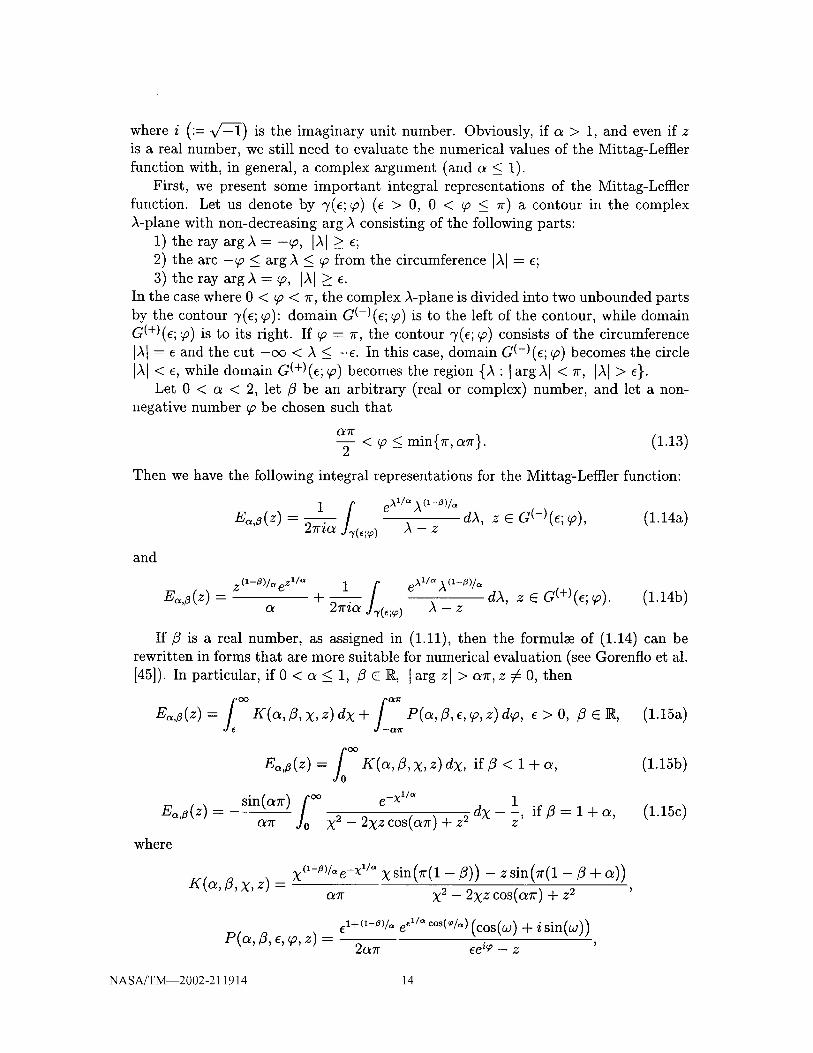
where i (:= v/-Z-1) is the imaginary unit number. Obviously, if a > 1, and even if z

is a real number, we still need to evaluate the numerical values of the Mittag-Leffier

function with, in general, a complex argument (and a _< 1).

First, we present some important integral representations of the Mittag-Leffier

function. Let us denote by 7(e; _) (e > 0, 0 < _ _< _r) a contour in the complex

A-plane with non-decreasing arg A consisting of the following parts:

1) the ray arg A = -T, IAI>_ e;

2) the arc -_o <_ arg A _< _o from the circumference IA[ = e;

3) the ray arg A = _, IAI_>e.

In the case where 0 < _o < % the complex A-plane is divided into two unbounded parts

by the contour 7(e; _o): domain G(-)(e; _) is to the left of the contour, while domain

G(+)(e; _o) is to its right. If _ = 7c, the contour 7(e; _) consists of the circumference

]AI = e and the cut -cx_ < A _< -e. In this case, domain a(-)(e; becomes the circle

IAI< while domain G(+)(e; _o) becomes the region {A largAI < IAI> 4,Let 0 < a < 2, let fl be an arbitrary (real or complex) number, and let a non-

negative number _o be chosen such that

o/Tr

-_- < _o _< min{% alr}. (1.13)

Then we have the following integral representations for the Mittag-Leffler function:

and

Ec_,_(z)- 27ria (e;_)

e)% 1/a A (1--/3)/t,

A--Z

dA, z E G(-)(e; _), (1.14a)

Ec,,Z(z) - z('-_)/_e_/"a + _I f_(,;_,) e:¢/_'A(_-z)/'_A-z dA, z E GC+)(e; _o). (1.14b)

If _ is a real number, as assigned in (1.11), then the formulm of (1.14) can be

rewritten in forms that are more suitable for numerical evaluation (see Gorenflo et al.

[45]). In particular, if 0 < a _< 1, _ E R, [arg z] > a_r,z ¢ 0, then

FE,_,Z(z) = K(a, j3, X.,z)dx +otqr

P(a,_,e,_,z)d_, e>0, /_eN, (1.15a)

f0 °E,_,_(z) = K(a,/3, X,z)dx, if/_ < 1 + a,

E,_,_(z)- sin(alr) f0 °° e -x_/_" 1O/.'lr )_2 __ 2XZ cos(azr) + z 2 dX - -'z if _ = 1 + a, (1.15c)

where

(1.15b)

K(a, _3, X, z) = X('-_)A' e-X'/_' X sin(_r(1 -/_)) - z sin(zr(1 - _ + a))a_ X2 - 2,z cos(a_-) + z 2

(cos( ) + i sin( ))P(a, _, e, _, z) = 2aTr ee i_ - z

NASA/T_2002-211914 14

= 1/osin( /o) + +The representations in (1.15), and similar formulae for the cases l arg z I = c_r and

f arg z I < a_r presented in Gorenflo et al. I45], are an essential part of the numerical

algorithm listed in the next sub-section.

Using the integral representations in (1.14), it is not too difficult to get asymptotic

expansions for the Mittag-Leffler function in the complex plane. Let a < 2, _ be an

arbitrary number, and _o be choosen to satisfy the condition (1.13). Then we have,

for any p E N and [z[ --+ oo:

1) Whenever [argz I _< _,

Z (1-/3)/° ezl/°

E_,_ (z) - (1.16a)C_

P z-k

r(A: + °(Izl-l-P)k=I

2) Whenever _ ___[argz I _< _-,

P z-k

Ea,_(z) = - E F(5---ak) + O([z[-1-P)" (1.16b)k=l

These formulae are also used in our numerical algorithm.

Thorough discussions of properties of the Mittag-Leffier function can be found,

for example, in Refs. [31, 76, 86].

1.5.2 Numerical Algorithms

Robust

The numerical scheme listed in Alg. 1.4 for computing the general Mittag-Leffier func-

tion E,_,_(z) is taken from an obscure paper written by Gorenflo et al. [45]. Their

algorithm uses the defining series (Eqn. 1.11) for arguments of small magnitude, its

asymptotic representation (Eqn. 1.16) for arguments of large magnitude, and special

integral representations (the formulae in (1.15) for the case where l arg z I > a_, and

similar representations for the cases l arg z I = c_ and l arg z I < a_) for intermediate

values of the argument that include a monotonic part f K(c_, _, X, z) dx and an os-

cillatory part f P(c_,/_, e, ¢, z) de, which can themselves be evaluated using standard

techniques (cf. App. B).

Efficient

Algorithm 1.4 can produce a numerical result to any desired level of accuracy, but

these computations are expensive and therefore their use in a finite element setting, for

example, is prohibative. To meet this need, we have constructed a table of Pad_ ap-

proximates for E_(-x a) in App. C for x __ 0 and c_ E {0.01, 0.02, 0.03,..., 0.98, 0.99}.

As we shall see in the next chapter, this form of the Mittag-Leffier function arises in

many fractional-order, viscoelastic, material models, including those of interest to us.

Another algorithm for solving the Mittag-Leffler function E,_(x) (0.02 < c_ < 0.98

with a reported relative error that is less than 1.6 x 10 -5) has been published by

Welch et al. [109].

NASA/T_2002-211914 15

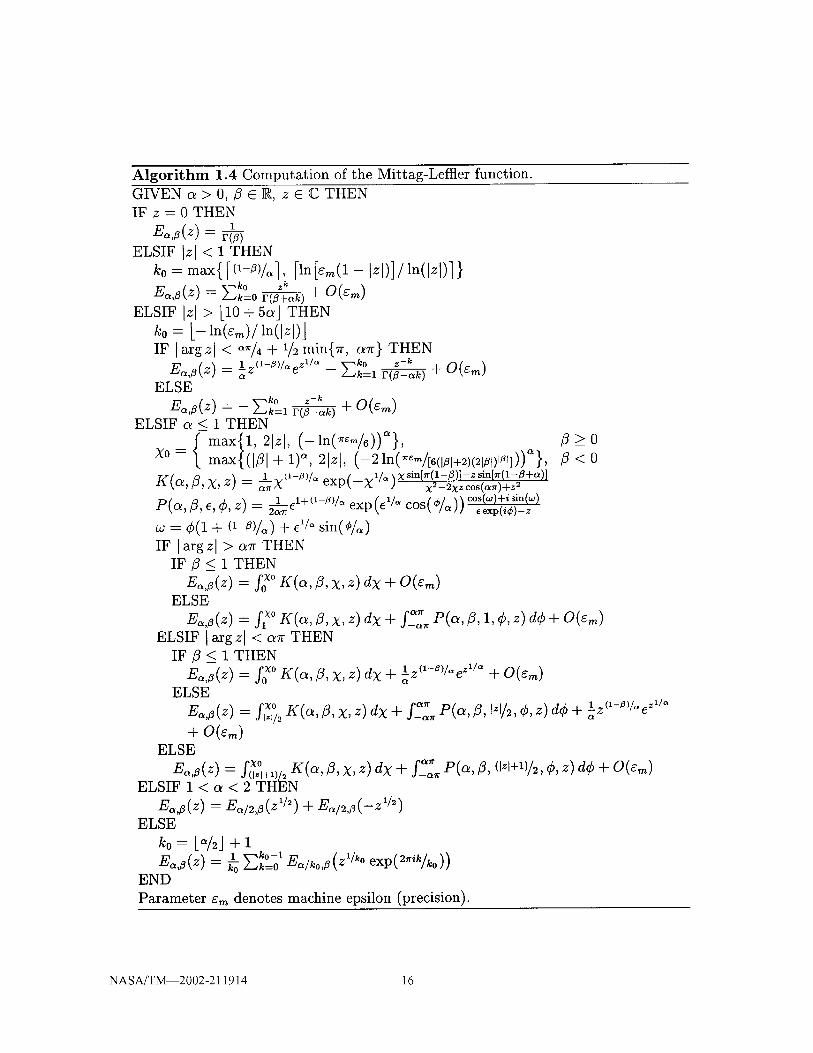
Algorithm 1.4 Computation of the Mittag-Leffler function.

GIVEN a > 0, /3 E R, zECTHENIF z = 0 THEN

E_,z(z) = 1r(_)ELSIE Iz[ < 1 THEN

ko -- max{[(1-zGl, [ln[_m(1- Izl)]/ln(Izl)l}ko z k

G,_(z) = Ek=0 r(_+ok)+ O(_m)ELSIE Iz[ > L10 + 5a] THEN

k0 = L-ln(_m)/ln(]zl)]IF larg z[ < _ff4 + 1/2 min{_, a_} THEN

E_,,n(z) !z(1-')/_'e z'° ko _-_= a -- Ek=l F(fl--ak) -t- O(Cm)

ELSEko z -k

E_,,(z) = - E_=I _(_-_,_1+ O(c.,)ELSIE a < 1 THEN

max{l, 21zl,(-ln(_m/6))_}, -_,x0 = max{(lfll + 1) _, 21zl, (-21n(_"/[_(lPl+2)(21Zl)'_l])) },

K'(_, ]3, X, z) = a-_X O-_>/_ exp(--X 1/_' "1x sin[w(1-_)]-z sin[_r(1-fl+a)]J X _-2xz cos(a_r)+z 2

P(a, Z, e, ¢,z) = 2--_el+(1-n)/'=' exp(e 1/_ cos(¢//a))c°s(w)+isin(w)

= ¢(1 + (_-,)/o) + _'/osin(G )IF [arg z[ > a_r THEN

IF/3 _< 1 THEN

G,_(z) : fo_°K(_,9,_,z)d_ + 0(_.,)ELSE

fl_>o

fl<o

E,_,n(z) = fl_°K(a,_,X,z)dx + f2_ P(a,_,l,¢,z) d¢+O(em)

ELSIE [arg z I < a_ THEN

IF _ < 1 THEN

E,_,n(z) = f_o K(a, fl, X,z)dx + lz('-_)l"e y_' + O(er,,)ELSE

E,_,n(z) =/i,xi}_ K(a, _, X, z)dx + f___,,_P(a, _, 1:1/2, ¢, z)de + -}z(_-')l:e y°

+o(_m)ELSE

fair P(aE,_,_(z) = f(_+_)/_ K(a, fl, X, z) dx + J-a,_ _ , fl, (Izl+l)/2, ¢, z) de + O(¢m)ELSIF 1 < a < 2 THEN

Ea,_(z) = E_12,f_(z 11') + E,_12,_(-z 112)ELSE

ko= L_/_J+ 11 _-_ko-1 E,_/_o3(ZV_ o exp(_.,_ik/_o) )Ea,z(z) = Vo z--.,k:O

END

Parameter sm denotes machine epsilon (precision).

NASA/T_2002-211914 16

Chapter 2

1D FOV

In the 1940's, Scott Blair [8] and Gerasimov [42] independently proposed a material

model bounded between a Hookean solid (c_ = 0) and a Newtonian fluid (c_ = 1).

Their relationship--a fractional Newton model--can be written as a(t) = #_-aD_e(t),

where a and e denote stress and strain, respectively, which are considered here to be

causal functions of time t. The coefficient #_- (> 0) represents a single material

constant (a generalized viscosity: # has units of stress, while _- has units of time),

and exponent c_ (0 < c_ _< 1) can be considered as a second material constant.

Experimental results motivated Scott Blair's model development. Mathematics, on

the other hand, motivated Gerasimov who was the first to consider an Abel kernel

for the relaxation modulus in Boltzmann's general theory of viscoelasticity.

Bagley and Torvik [4] demonstrated that the molecular theory of Rouse (for dilute

solutions of non-crosslinked polymer molecules residing in Newtonian solvents) has

a polymer contribution to stress that corresponds to a fractional Newton element

whose order of evolution is a half (i.e., a = 1/2). They also state (without proof) that

the molecular theory of Zimm (for dilute solutions of crosslinked polymer molecules

residing in Newtonian solvents) has a polymer contribution to stress that corresponds

to a fractional Newton element whose order of evolution is two thirds (i.e., c_ = 2/3).

Gemant [38] was the first to propose a fractional viscoelastic model. He extended

the notion of a Maxwell fluid by replacing its first-order derivative on stress with the

semi-derivative, and in doing so, he proposed that [1 + v/_D_/2]a(t) = riDe(t),

where # (> 0) and rl (> 0) are material constants. The fractional Maxwell fluid,

which is a spring in series with a fractional Newton element, actually has the form

77 (2.1)[1 + r=D_]a(t)=rITa-lD_e(t), cro+ = -eo+,T

where r1 (> 0) is the viscosity, r (> 0) is the characteristic relaxation time, and

exponent c_ (0 < c_ < 1) is the fractal order of evolution, which is taken to be the

same for both stress and strain, while (r0+ and e0+ are the initial states of stress

and strain at time t = 0 +, thereby allowing for an inhomogeneous initial state of

finite stress--a characteristic that Gemant's model does not possess. The fractional

Maxwell fluid was first discussed in the manuscript of Caputo and Mainardi [13] as

a special case to their material model (Eqn. 2.2 below). We refer to (2.1) as the

standard FO V fluid in 1D.

NASA/T_2002-211914 17

Caputo [12] introduced a fractional Voigt solid a(t) = #[1 + paDa,]s(t) to model

the nearly rate-insensitive dynamic response of Earth's crust over large ranges in

frequency when excited by earthquakes. Here # (> 0), p (> 0) and a (0 < a < 1)

are the material constants. As a mechanical model, this is a spring in parallel with

a fractional Newton element. A more appropriate representation of solid behavior is

the fractional Kelvin model, which is a spring in parallel with a fractional Maxwell

element. This material model was introduced by Caputo and Mainardi [13] and hasthe form

[1 + _-_D_,]a(t) = #[1 + p_D_]e(t), a0+ = # ¢0+, (2.2)

where # (> 0) is the rubbery modulus, #(p/7-) _ (> tt) is the glassy modulus, _- (> 0)

is the characteristic relaxation time, p (> _-) is the characteristic retardation time,

and exponent a (0 < a <_ 1) is the fractal order of evolution. This model, unlike

Caputo's original model, allows for an inhomogeneous initial state of finite stress.

Bagley and Torvik [5] have shown that the fractal orders of evolution in stress and

strain must be the same, as written in (2.2), and as originally proposed by Caputo and

Mainardi, in order for this constitutive realationship to be compatible with the second

law of thermodynamics; specifically, in order to guarantee a non-negative dissipation

whenever a cyclic loading history is imposed on the material. We refer to (2.2) as the

standard FOV solid in 1D, in the spirit of Zener [111, pg. 43] referring to Kelvin's

model [1 + TD]a(t) = #[1 + pD]s(t) as the "standard linear solid".

The initial conditions present in (2.1 & 2.2) come about by taking the Laplacetransform* of these constitutive formulae. What one learns from these transformations

is that if the material model is to be physically admissible, in the sense that it

propagates a wave front at finite speed, then that part of the transformation which

pertains to the initial state must be independent of the Laplace transform variable s in

the frequency domain, or it must have like dependencies on both sides of the equation

*The Laplace transform ](s) of function f(t) is given by the mapping procedure f(t) + if(s) =fo exp(-s_-) f(T) d_', where .'- denotes the juxtaposition of function f(t) with its Laplace transform](s). In fractionM-order viscoelasticity, the Laplace transform pairs

L_J tn-1D_f(t)--saf(s)- _ ._a-k-1_(k) 1 Sa-:_

A._- Jo+, r(n) -s n and t/_-l Ea,/3(:Eat a) " sa T ak----0

have particular significance, where ce,a,n, t 6 _-, _ E _ and Ea,/_(t) = _=o tk/F(_ + ak) is thegeneral Mittag-Leffier function, which plays a role in FDE's like that which the exponential functionplays in ODE's; in fact, El,l(t) = e t.

The above formulae are analytic continuations of the well known Laplace transform pairs

m--i tin_ 1

Dmf(t) + s'_i(s) - E :_-k-1 ,(k) 1 1]0+' (m-1)! " s m and e ±at - ,

k=0 S =F a

where m E N and a, t E ]l_+. In contrast to the Laplace transform of Caputo's deriviative, whichcontains a sum of integer-order derivatives of the initial state, the Laplace transform of the Riemann-Liouville derivative contains a sum of fractional-order derivatives of the initial state, making theinitialization of Riemann-Liouville based differential equations a difficult task, but not an impossibleone [73].

NASA/T_2002-211914 18

that thencancelout in the initial state. Havingderivativesof equalorderonboth sidesof the equation,as in the standardFOV fluid and solidmaterial models,is onewayto ensurethat this physicalconstraint is adheredto. In the aerodynamicsliterature,this processof addressingthe initial state for consistencyof initial condition in thefrequencydomain is knownasthe method of shocks,which wasintroduced into theFOV literature by Bagleyand Calico [3]. Another very important reasonto restrictthe classof admissiblematerial modelsto only includethose that propagatewavesat finite speedshas to do with stability. Material modelsthat predict infinite wavespeedswill becomemathematicallyunstableat somecritical finite velocity [65].

Oneobjectiveof this paper is to derive3D versionsof the standard, FOV, fluidandsolid, material modelswithout imposingany constraintsasto the magnitudeofdeformation.To the best of our knowledge,Drozdov[27]is the only personto haveextendedlinear, fractional-order,viscoelasticformulationsinto 3D formulmapplicableto non-linearmechanicswherefinite strains are present. Specifically,he extendedthe following ID models: [I + (71/#)_Da,]a(t)= r]D_(t), which is a generalization

of Gemant's [38] fractional Maxwell model, and a(t) = #[1 + p_D_]e(t), which is

Caputo's [12] fractional Voigt model. In Chps. 7-??, we introduce 3D versions for

the standard FOV fluid and the standard FOV solid, which are presented here in 1D

in Eqns. (2.1 & 2.2).

2.1 Material Functions

The parameterization procedures that follow assume infinitesimal strains in homoge-

neous ID deformations.

Boltzmann's [9] linear theory of viscoelasticity, which includes the standard FOV

models of (2.1 & 2.2), can be expressed as an integral equation with a hereditary

kernel that convolves with a change in the independent state variable according to

the convolution rules of either Stieltjes or Riemann. Whenever stress responds to

strain, this theory can be expressed in terms of a (relaxation) modulus G(t) where

[16, pp. 3-9]

I' /oo(t) = a(t - t') de(t') = eo+a(t)+ a(t - t') Os(t') at', (2.3a)+

or conversely, whenever strain responds to stress, Boltzmann's theory can be re-

expressed in terms of a (creep) compliance J(t) where

f0 /:e(t)= J(t-t')da(t')=ao+J(t)+ J(t-t')Dcr(t')dt'. (2.3b)+

These two convolution integrals can be solved analytically using Laplace transform

techniques, provided that the loading histories are simple enough.

The standard FOV fluid (2.1) has a modulus a(t) and a compliance J(t) of [131

a(t)= T G(--(t/T) °)

( (,/T)_ _ , (2.4)J(t) = _ 1 + I'(1 + c_)]

NASA/T_2002-211914 19

whereas,the standardFOV solid (2.2)has the material functions [13]

((;)oa(t) =, + Eo(--('/T)°

where E_(x)= E,_,l(x)is the Mittag-Leffier function (see §1.5).

(2.5)

2.1.1 Static Experiments

Stress relaxation experiments are often executed for the purpose of materials charac-

terization, where

for standard FOV fluids,

for standard FOV solids.(2.6)

Figure 2.1 presents a normalized plot of stress relaxation curves for the standard

FOV fluid, with a = 1 designating the response of a classic Maxwell fluid. The

stress relaxes to zero monotonically in a FOV fluid for all a E (0, 1]. Figure 2.2

presents a normalized plot of stress relaxation curves for the standard FOV solid,

with a = 1 designating the response of a classic Kelvin solid. For all a C (0, 1], the

stress monotonically relaxes to a unique non-zero value in a FOV solid as t --+ c_,

which distinguishes solid behavior from fluid behavior. Here, and in the following

figures of this chapter, the relaxation _- and retardation p times are assumed to scale

as (@)_ = 5 for purposes of illustration. These figures show that the fractal order of

evolution controls the shape of the relaxation curve.

Relaxation, as described above, exhibits an exponential decay as t -+ c_ when-

ever a = 1, and an algebraic decay to infinity whenever 0 < a < 1. This corresponds

to a regular rate process leading to strong mixing (exponential decay) versus an in-

termittent rate process causing weak mixing (algebraic decay), as quantified by a

probabilistic fluctuation of recurrent events (molecular collisions) governing the ve-

locity relaxation process in polymer chain physics. Douglas [25] has shown, through

probabilistic reasoning using Feller's renewal theory, that the autocorretation function

describing relaxation phenomena is governed by a fractional-order differential equa-

tion whose solution is given in terms of the Mittag-Leffier function, and whose order

of evolution correlates with the degree of intermittency in the relaxation process.

Douglas [25] also states that the stretched exponential, e.g., exp(-(t/T)'_), often

used to empirically fit relaxation data in the literature, does not arise from probabilis-

tic considerations in polymer chain physics. Popularity of the stretched exponential

over the Mittag-Leffier function has two likely sources: many researchers are not fa-

miliar with, or have even heard of, the Mittag-Leffler function, and if they are familiar

with it, they do not likely know how to compute its value. With respect to the latter,

see Alg. 1.4 and App. C.

NASA/T_2002-211914 20

E._9t-a

O

O

Z

0.8

0.6

0.4

0.2

00

Relaxation Modulus: Standard FOV Fluid[1 + _D,_]_(t) t_

=_x D,e(t)

' I ' I ' I ' I '

..... (x = 0.25

.... ix = 0.5

--- ot = 0.75

I-- a=l

_._\_

2 4 6 8 10

Normalized Time, t / x

Figure 2.1: Normalized diagram for stress relaxation of a fractional Maxwell fluid.

eJ

Q.

O

o

0.8

0.6

o

"_ 0.4

(x/p) _ = 0.2

Z

Relaxation Modulus: Standard FOV Solid[1 + xaD,_]er(t) = Ix[1 + paDa,]e(t)

' I ' I ' I ' I '

..... _X= 0.25 [

.... _=o.5 I, --- c_ = 0.75 I

I

71 i_UL2?7;

0 , I , I , I , I ,0 2 4 6 8 10


Figure 2.2: Normalized diagram for stress relaxation of a fractional Kelvin solid.

NASA/T_2002-211914 21

10

Creep Compliance: Standard FOV Fluid[1 + _D._lcr(t) = t_-Ifix D, e(t)

O

e_

r,.)

"N

.eO

Z2

1

00

' I ' I ' I ' I J'J

--a=l-

--- c_= 0.75 _

.... _=0.5 _"

..... U* _ U.LJ

.......... i

, I , l , I , I ,

2 4 6 8 10


Figure 2.3: Normalized diagram for creep of a fractional Maxwell fluid.

Creep experiments are also performed for purposes of materials characterization,

where

e(t) + r(-(7-4_)(t/T)'_ for standard FOV fluids,- .° To, (2.7)

e0+ + _[1 - E_(-(%) _) for standard FOV solids.

Figure 2.3 shows a normalized plot of creep curves for the standard FOV fluid. A

specimen will creep without bound in a FOV fluid for all a E (0, 1]. However, only

in the case of a Maxwell fluid where c_ = 1 is the 'effective' viscosity (i.e., the slope)

a constant. Conversely, FOV fluids will eventually (at infinite time) stop creeping

altogether (see Eqn. 2.9). Figure 2.4 shows a normalized plot of creep curves for the

standard FOV solid. Here creep stops at a unique threshold level in strain for all

a E (0, 1]. Steady-state creep behavior cannot be predicted by this class of material

models. The fractal orders of evolution influence the shape of these curves, too, and

in the case of a solid, they also influence the time required to attain saturation.

It is difficult to parameterize an FOV solid with only relaxation data, or with only

creep data. This is because it is difficult to acquire sufficient sensitivity in the data

to the parameter p in the case of relaxation, or to the paramter T in the case of creep.

But whenever relaxation and creep data are used together during estimation, ample

sensitivty will exist for all material constants and good data fits can be expected.

Although Figs. 2.1-2.4 are informative, they are not as practical as one would like

in the sense that one cannot directly extract the order of evolution, a, from them via

some graphical technique. However, if one were to measure stress rates in a relaxation

experiment, or strain rates in a creep experiment, then the order of evolution could,

NASA/T_2002-211914 22

Q.

::k

g

o

Z

Creep Compliance: Standard FOV Solidc_ c_ t 9_D,a]e(t)[l+x D.lo()=g[l+

1t .....0.8

s _... ....j- .._.....

0.6 .._._.//

;1!

; ;/;//

0.4 .!/

.... o_ = 0.5

i -- o_=1

--- _ = 0.75

(_:o7= o.z t I..... _ = °-251

01 , I , I , I , I0 2 4 6 8 10

Normalized Time, t / 13

Figure 2.4: Normalized diagram for creep of a fractional Kelvin solid.

in theory, be extracted as a slope in an appropriate log-log plot of the data. In a

stress relaxation experiment

Da(t) _ _ DE,_(-(t/-_) _) for standard FOV fluids, (2.8)

ao+ [e£-S_DE,_(-(t/,)'_ ) for standard FOV solids,

whereas, in a creep experiment

De(t) ( _ r_/ _1-_

eo+ l_ DE,_(-(%) _')

for standard FOV fluids,

for standard FOV solids.(2.9)

Figure 2.5 presents a graphical representation of OE,_(-x_)/Ox, t which appears in

three of the four descriptions above, with the exception being creep rate in a standard

FOV fluid, which has a power-law response. Cureously, what is observed in Fig. 2.5 is

that OE,_(-x'_)/Ox approximates power-law behavior whenever x < 0.1. The scheme

depicted in this figure for extracting a is accurate (to two significant figures) over

the range of 1 <_ c_ <_ 1/2, but it looses accuracy as a approaches zero; for example,

this graphical scheme yielded a value for a of 0.27 when it was actually 1/4. Even so,

tFrom Podlubny [86, pp. 21-22], one finds that

OE_,_(-(_/y) _) = Eo,0(-(%)_)OX X

for0 < a < 1, x > 0 and y > 0.

NASA/T_2002-211914 23

Derivative of the Mittag-Leffier Functionx

0-6 10 .5 10-4 10 -3 0.01 0.1 1,4

-....' I ' L ' I ' I ' I ' I '

L ............. .r-..- g= 0.25

I-. "........ I--- a=0.5/ .......... "........ I--- a=o.75

2_- .... " ..... '"". I---- a= 1

-2 1 - a

1

-4 , I , I , I , I , I , I ,-6 -5 -4 -3 -2 -1 0

Log(x)

lOo4

10 2

-?

10-2

10 "4

Figure 2.5: Diagram of the derivative of the Mittag-Leffier function, OE_,I (-x_)/Ox =

this is likely to be accurate enough for material characterization purposes given the

uncertainty of experiemental error. Because the time constant for creep is typically

many orders of magnitude greater than the time constant for stress relaxation, it will

be easier to satisfy a boundary of x < 0.I in a creep experiment than it would be to

satisfy it in a relaxation experiment; nevertheless, the experimental challenge remains

great.

2.1.2 Dynamic Experiments

Also useful for the purpose of materials characterization are dynamic experiments

where strain is controlled at a constant amplitude s0 and angular frequency w ac-

cording to e(t) = e0 exp(iwt), to which stress responds with a dynamic modulus of

G*(w) = G'(w)+iG"(w) such that a(t) = soG*(w)exp(iwt). The real G'(w) and imag-

inary G"(w) parts of the dynamic modulus are called the storage and loss moduli,

respectively, whose ratio, tan 5(w) = G"(_)/C,(_), is often reported in the literature.

Figure 2.6 illustrates how these properties are extracted from experimental data ob-

tained under steady, oscillatory, loading conditions, where the stress-strain curve is an

ellipse with control 6(t) = e0 sinwt and response a(t) = ao sin(wt + 5). A material is

non-linear if the hysteresis is something other than an ellipse under sinusoidal loading

conditions. A thorough discussion of dynamic experiments, as they relate to linear

viscoelastic materials characterization, can be found in the recent text by Lakes [62,

Chp. 3].

NASA/T_2002-211914 24

C o

G' Eo ............

E

Figure 2.6: Extracting dynamic properties from linear viscoelastic materials.

For the standard FOV fluid (2.1), the dynamic modulus is given by

a*(w) = _- (iw_)°_- 1 + (iwT) _'

whose real and imaginary parts are

a'(_) _ (_)o +_s(o_l_) }= ; (_) ¥_£q-_+2_(°%)

sin(_h) 'a"(_) = 7 (_)o + (_)-o + 2cos(_/2)

and that ratio as sin(_/2)

tan _(_) = (_)_ + cos(o%)

For the standard FOV solid (2.2), the dynamic modulus is given by

G*(_)= _ 1+ (i_-)o'

whose real and imaginary parts are

(p)a (wg-) _ + (wp) -_ + (1 + ('@)a)cos(_/2)la'(_) = _ .,. (_)_ + (_)-o + 2cos(_12)

(p)a (1-(r/°)a)sin(a'/2) IG"(_) =. (_)o + (_)-_ + 2cos(_%)

NASA/T_2002-211914 25

(2.10a)

(2.lOb)

(2.10c)

(2.11a)

(2.11b)

0.6

-_ 0.5

(9 0.4

8 0.3

O..A

-o 0.2

._

O7 0.1

Cole-Cole Plot: Standard FOV Fluid[1 + "_D.a]o(t) = _-1q_ D.e(t)

' I ' I ' I ' I ' I '

00

--- c_= 0.75.... (x = 0.5

= 0.25 I

1iI I" .. • "_

.,..,.. -.. x. % I

0.2 0.4 0.6 0.8 1

t1.2

Normalized Storage Modulus, -c G'('_co;o_) / q

Figure 2.7: Normalized Cole-Cole diagram for a fractional Maxwell fluid.

and that ratio as

(1- (_/p)_) sin(_/2)

tan6(w) = (w__)_ + (wp)__ + (1 + (_/p)_) cos(_/2)'(2.11c)

thereby requiring _- < p if G" > 0--a well-known requirement of thermodynamics--

given that#>0,_->0, and0<a_l.

A Cole-Cole [17] diagram--a plot of G'(c_) versus G'(a_)--is a very sensitive way to

view anomalous relaxation phenomena. Figure 2.7 presents the normalized Cole-Cole

diagram for the standard FOV fluid, with the a = 1 curve designating the response of

a Maxwell fluid. Figure 2.8 presents a normalized Cole-Cole diagram for the standard

FOV solid, which in this case translates the storage modulus of the FOV fluid by an

amount (_/p)_ = 0.2, with the a = 1 curve designating the response of a Kelvin solid.

The influence that the fractal order of evolution has on material response is readily

apparent in a Cole-Cole diagram. Fractal order affects the extent of dissipation.

Cole-Cole-type relaxations are naturally produced by random-walk models done

on fractal lattices brought about by studying the motion of a particle in restricted

geometries [37]. They also result from random-walk models done in fractal time on

regular lattices, where the probability distribution is now a decaying power-law in

time instead of the more common decaying exponential [43]. Random walks are used

to establish the mean-square end-to-end distance of polymer chains in the various

statistical theories of polymer physics, both for fluids and solids (e.g., cf. Douglas

1251).

NASA/T_2002-211914 26

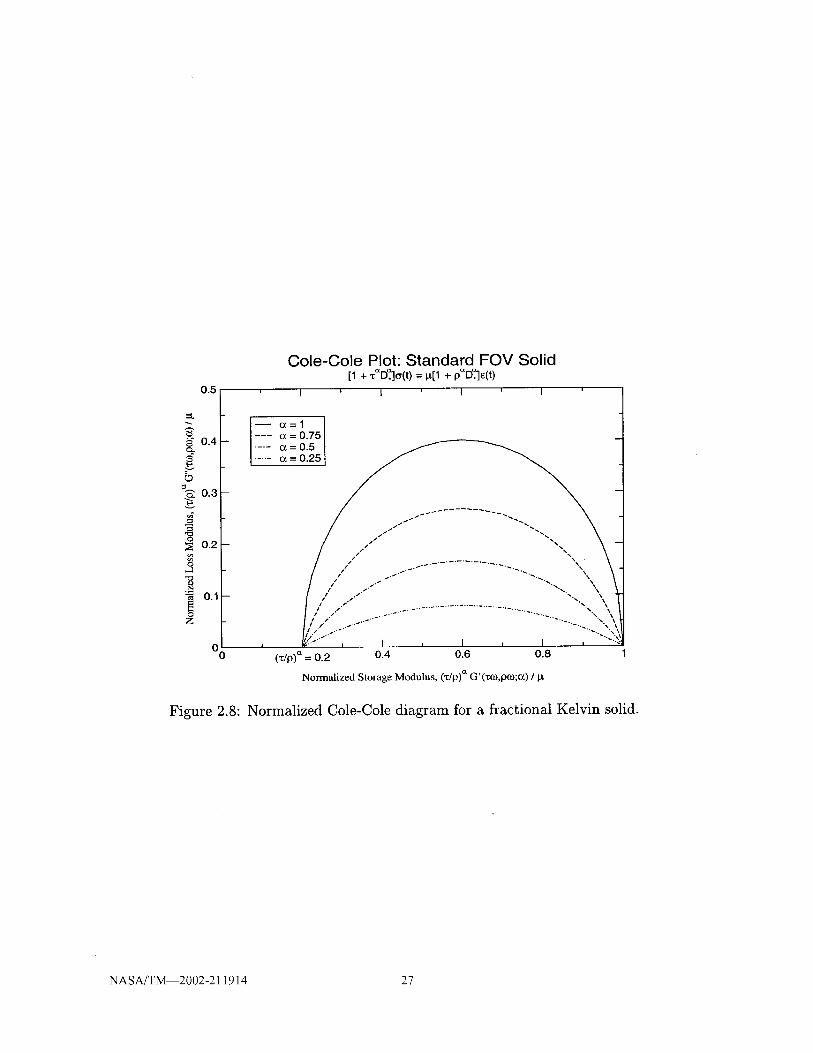
0.5

=:L

£" 0.4

b0.3

o

0.2

.9

o.1

QZ

0 o

Cole-Cole Plot: Standard FOV Solid[1 + "_D_.]a(t) = g[1 + p_D_e(t)

I ' I ' I ' I

[_ (z=l

(z = 0.75c_= 0.5

0_----

i / .....

I

('dp) '_ = 0.2 0.4 0.6 0.8

Normalized Storage Modulus, (_/p)_ G'(xto,po};(_) / Ix

Figure 2.8: Normalized Cole-Cole diagram for a fractional Kelvin solid.

NASA/T_2002-211914 27

Chapter 3

Continuum Mechanics:

body-tensor fields

In this report we use body-tensor fields (as defined by Lodge [68, 69, 70]) for deriving

constitutive formula_, and we use Cartesian space-tensor fields (as commonly used

throughout the literature) to solve boundary-value problems. In this regard we are

free to select the tensor analysis scheme best suited for a particular task at hand,

since one can readily map body-tensor fields into space-tensor fields, and vice versa.

In this chapter we present the basic fields used in body-tensor analysis. In the next

chapter we map these fields into Cartesian space, thereby producing tensor fields that

are likely to be more familiar to the reader.

Consider a continuum consisting of an infinite set of point particles, {_3}, also

referred to as mass elements, that fills a domain, B, in 3-space (B C JR3). We call

this set the body B. In any admissible body-coordinate system, B, defined over B,

each particle _ in B is assigned a unique set of body coordinates, _ : (_1, _2,_3),

_ C N, that are independent of time (i.e., B: _3 -+ [, cf. Lodge [69]). In this sense,

body-coordinate systems have been construed as being convected coordinate systems.

3.1 Metric Fields

The distance dS separating any two neighboring particles--say, _ and _--in B can

be quantified by using the covariant body-metric tensor, _, of Lodge [68, 70] that he

assigned to a Riemannian manifold with geometric measurement

(dSo) 2 = d_ " _o" d__ and (dS) 2 = d_ "l " d_, (3.1)

where __(_; t) is symmetric positive-definite and, most notibly, a function of time t

with __0 := _(_; to), wherein to is usually taken to be zero (0). This tensor field has

a matrix representation of _ (= I7_cl; r, c = 1, 2, 3) in the coordinate system B with

components 7_j = Yj_ = 7_j([; t). Scalar dS(gt3; t) is the infinitesimal length-of-line of

the contravariant vector d__(_) := _, with dSo := dS(_;to) designating its gauge

length.

NASA/T_2002-211914 29

A singledot placedbetweentwo tensor fields representsa contractionoveronearray index. Likewise,adoubledot (colon)will representa contractionovertwoarrayindices.

3.1.1 Dual

Becausethe metric tensor3' is symmetricpostitive-definite,it hasa dual--the con-

travariant (inverse)body-metric tensor,_-1(q3;t)--whose matrix representation _3-1

(= lTrcl) has components 7 ij = 7 ji = 7iJ(_;t) in B such that _-1..y = _, where

_(q3) is the mixed idem tensor with a matrix representation of $ (= I5_) possessing

components 5} that equal 1 whenever i = j, or that equal 0 whenever i 7_ j, in everybody-coordinate system.

This dual body-metric tensor, ,),-1 has two possible geometric interpretations.

In the first interpretation, provided by Lodge [68, pg. 318], the distance dH(q3;t)

measuring the height-of-separation between any two, neighboring, material surfaces--

say, a(__) = C and a(__ + d_) = C + dC, where C and dC are constants--belongingto the same one-parameter family of non-intersecting surfaces, a, in _ is quantified

via the contravariant body-metric tensor, _,-1, according to

dC _ 2 Oa 0odgo ] = _ " 7=°1" _ dC) 2 Oct . _-1.00 &r . d_, (3.2)and _ = _ = _-_, dC= O---_ -

where (Ocr/O__)(q3) is a covariant vector, independent of time t, that is normal to

this material suraface, with contravariant vector d_ originating on one surface and

terminating on the other. Scalar dHo := dH(_; to) is the gauge length for this height-

of-separation, while __o1 := 7_-1(q3; to).

A second geometric interpretation for the dual metric, provided by Truesdell [108]

in an analysis done using general space-tensor fields, has a description of

____-_1_ _..__--1

• (d__×__) and (dA)2=(d_x_)det_,_l-(d__×__),(dAo) 2 = (d_ × _--) "det 7__o1

(3.3)

where det _, denotes the determinant of % which is a scalar field with a tensorial weight

of two (2), and therefore the areal metric tensor, (det _) _,-1, is a relative field of like

weight. Scalar dA(_; t) is an infinitesimal area-of-surface, with dAo := dA(_;to)

designating its gauge area. This material surface contains neighboring particles 9,

_, and _". The normal to this surface lies in the direction of a covariant vector fieldA

given by the cross product d_ × d_, which has a tensorial weight of minus one (-1),

wherein d__(_):= q3_ and __(q3)-= q3_ _.

The unit normal u__(q3;t) to element dA is given by u_dA := dv/-d--_3, d_ × d_'_. This is

an 'absolute' (without tensorial weight) covariant vector that, in bod_ tensor analysis,

is a function of time t through the presence of _,(q3; t), because Ilzl? ==z.7-1.z = 1.

NASA/T_2002-211914 30

3.1.2 Rates

The various descriptions for strain rate that are found in the literature can all be

expressed in terms of derivatives of the metric tensor, _, its inverse, "7-1, and its

determinant, det _'. The time rate-of-change of the body-metric tensor, D'7, is defined

classically through the limiting process

-_(_;t) - __(_;t')D-)'(_3; t) = lim = t' (3.4)tl -+ t t -- '

while the time rate-of-change of the determinant of the body metric, D(det'),)(_; t),

is given by

D(det _) = (det "Y)(tr D__), (3.5)

wherein the trace, tr D'y, is computed as "7-1" D'),, consistent with the precepts of

general tensor analysis.

The first-order body-metric rates D_(_; t) and D_-1(_3; t) are not independent.

Instead, they are related through the expression

O0,-1 = _.y-1. (D'7)- _-1. (3.6a)

Likewise, the second-order rates D2"7(_; t) and D2"7 -1 (9; t) are related through

D2_,-I =.y-I. (2 (D_) .V-I. (D._) - (D2.),) ) .'y -1. (3.6b)

These identities are easily derived by applying the Leibniz product rule for differen-

tiation to the expression "7-1. _ = 5, noting that D_ = 0=. Higher-order relationships

can be acquired in like manner, but they are not needed in this work.

Fractional order

From the definition of Caputo differentiation (1.8a), one can compute fractal rates

for metric evolution via the formulm*

lfi }D_*2(_;t°'t) = r(1- a) (t Z-t,)_ (D2(_;t')dt'

- , (3.7)

D o -1 1 ftl 1 (p.y_l)(9_;t,)dt,,_ (_;t0, t)- F(1-a) (t--t') _ =

*Because (_) _ 0 whenever k > a given that k E N and a E 1R+with a ¢ N, the Leibniz productD, "y thanrule (1.7) applicible to the Caputo derivative (1.3) leads to a more complex identity for _ -1

otherwise exists in the integer case (3.6a); specifically, for 0 < a < 1,

(to- t)-_ _ (_ (j__o __)D_-_=- Y(i-:_ (__o__-__--_)- Z \k/ = •(D%)._-1,

k=l

where __o+z := .y-1 (_3; to+). Consequently, there is no direct relationship between D,a'y and D a- -1

These r-ate fiel-ds are independent of one another. This result follows from D.a("t -1. _) - D_6 = O.

NASA/T_2002-211914 31

where the fractal order of differentiation is restricted to the range 0 < a < I. Un-

like integer-order derivatives of the body metric (i.e., D_(_:_;t) and D_-1(_;t)),

which are one-state fields in time t, fractal-order derivatives of the body metrics (viz.,

D,__(_; to, t) and D,__-I(_3; to, t)) depend on all states traversed along the time in-

terval [to, t], where we shall typically take to to be zero in this work.

3.2 Strain Fields

Strain tensors are the preferred measures for describing deformations in solids, because

solids have a quantifyible reference state. On the other hand, metric tensors are the

preferred measures for describing deformations in fluids, becuase fluids have no uniquestate of reference.

Strains are two-state fields that ideally possess four characteristic properties. The

first property is: strain is a relative measure of deformation in that it vanishes when-

ever its two dependent states are coincident. The second property is: strain is addi-

tive and anti-symmetric in its dependency upon state. The third property is: strain

exhibits tension/compression asymmetry; for example, axial extensions of A and A-I

correspond to strains that are equal in magnitude but opposite in sign. And the fourth

property is: strain is an absolute field (i.e., without tensorial weight) although, for

the most part, this is really a requirement of convience. The second and third criteria

actually quite restrictive. Only Hencky strain is known to satisfy all four of thesecriteria.

The classic strain measures are defined below. The first two are tensor fields that

relate to two distinct changes in length-of-line; the first tensor relates to a separation

between neighboring particles, while the second tensor relates to a separation between

neighboring material surfaces. The third strain measure is a scalar field that relates

to the volume change of a mass element.

3.2.1 Covariant

The metric geometry of (3.1) can be rearranged in such a manner that (cf. Lodge [68,

pp. 24-261)

1,),(dS)2-(dSo)2= 2d_.e_.d_, e_:: i(_-_o), (3.8)

where __e(_; to, t) is an absolute, symmetric, covariant, strain tensor. It has properties:

i) tensor e__vanishes in the reference state, =e(_; to, to) = O; ii) it is additive and anti-

symmetric in its time agruments, e__(_; to, t) -- _e(_3; to, t') +__e(_; t', t) for all t' E [to, t],regardless of the extent of deformation; and iii)it has no tensorial weight; however, it

does not possess tension/compression asymmetry. Typically one sets to to zero, but

for the time being, we shall leave it as to for clarity of discussion.

The factor of 2 that appears in (3.8) is for historical reasons. Specifically, engi-

neering strain is given by (_-Q)/Q for the infinitesimal extension of a rod with length

_(t) whose gauge length is _0 := _(to). A normalized representation of the left-hand

NASA/T_2002-211914 32

sidein (3.8)producesthe relative strain measure

(as)2- (as0)2 (as + as0) (as - as0)2 (dSo) 2 2 dSo dSo

dS - dSo_ whenever

dSodS ,.., dSo,

(3.9)

demonstrating a consistency with the classic definition for engineering strain underconditions of infinitesimal deformation.

Rates

The covariant strain-rate tensor, D__e(_; t), is a one-state tensor field given by

De = 1 (3.10)= _ D__,

because D_'0 = O.

The covariant, fractal, strain-rate tensor, D___e(_; t0,t), depends on the path of

straining incurred over the interval [to, t] of integration, and is given by

D_,e = 1 _ (3.11)= 5 D*2,

(the Caputo derivative of a constant is zero).because D,_0 = O

3.2.2 Contravariant

In similar fashion to (3.8), the metric geometry of (3.2) can be rearranged in such a

manner that (cf. Lodge [68, pp. 26-32])

ffio/-1

__:= _("7o 1 - _-J), (3.12)

where _(_; to, t) is an absolute, symmetric, contravariant, strain tensor t, which pro-

vides another acceptable representation for strain. Like _e, the strain _ is: i) a relative

?From (3.3), one can likewise define an alternative, symmetric, contravariant, strain measure as

which is a relative measure of deformation in that 13(gl; to, to) = 0, and it is also additive and

anti-symmetric in its time agruments because/3(g1; to, t) =/3(_3; to, t') +/3(g1; t', t) for all t' E [to, t],

regardless of the magnitude of deformation; however, it has a tensorial weight of two (2). It canbe converted into an absolute field (i.e., without tensorial weight), but the outcome will violate thesecond desirable property of a strain field (viz., additive and anti-symmetric in state dependence).

Because tensorial weights must equal amongst all additive terms in a tensor equation, and becauseall of the other tensor fields that we happen to use in constitutive development are absolute fields, itis therefore not practical to use/3 as a strain measure, even though it has the desirable interpretation

of relating to changes in area-of-surface.

NASA/T_2002-211914 33

measureof deformationin that _(_; to, to) = O; ii) it is additive and anti-symmetric

in its time agruments because _(_;t0,t) = _(_;t0,t') + _(_;t',t) for all t' • [t0,t],

regardless of the extent of deformation, and iii) it has no tensorial weight; however,

it does not possess tension/compression asymmetry.

Rates

The contravariant strain-rate tensor, D_(_; t), is a one-state tensor field given by

1 (3.13)D__ = -_ D"y -1 -- _ _ ._

because D_o 1 = O.

The contravariant, fractal, strain-rate tensor, D_(_; to, t), depends on the path

of straining incurred over the interval [to, t] of integration, and is given by

1 a --1 (3.14)D_ = -b D,_ ,

a -1because D,__o = 0 (the Caputo derivative of a constant is zero). Unlike the integer-

order strain rates D_e and D4, there is no identity relating the fractal strain rate D,__e

to D._¢.

3.2.3 Dilatation

To acquire a volumetric strain measure that is additive and anti-symmetric in its

time dependency and exhibits tension/compression asymmetry, too, requires taking

a different tact. Using the conservation of mass as our guide (viz., integrating D In 0 =

I tr Dr) leads to Hencky's [50] definition for dilatation, A(_; to, t), which is a scalar2

field given by (cf. Oldroyd [83])

1 ln(det(zol" 2) = ln(00/Q) --=ln(dV/dVo).A=5 (3.15)

This is our third classic strain measure. Like the prior strain measures, dilatation: i)

vanishes in the reference state, A(_; to, to) = 0; ii) it is additive and anti-symmetric

in its time dependence, A(_; to, t) = A(_; to, t') + A(_; t', t) for all t' • [to, t], in-

dependent of the magnitude of deformation; and iii) it is without tensorial weight.

Unlike the two prior strain measures, it iv) possesses tension/compression symmetry

in that ln(dV1/dV2) = -ln(dV2/dV1).

Scalar Q(_; t) denotes the density of mass element 9, with _0 := Q(_I; to) being its

gauge density. Scalar dV(_3; t) is the infinitesimal volume of mass element _ at time

t, with dVo := dV(_3; to) denoting its gauge volume. Because det _o 1 has a tensorial

weight of minus two (-2), while det _ has a weight of plus two (2), it follows that

det(_o 1- V) has no tensorial weight, and therefore A is an absolute scalar field.

NASA/T_2002-211914 34

Rates

Dilatation A is actually defined via its rate, DA(_; t), according to the expression

1DA := _trD_ = -Dln_--DlndV, (3.16)

which arises from the conservation of mass. It has a fractal rate of D_A(_3;to, t),

where

1 ftl 1D_*A- r(1- c_) (t --t') _ (DA)(t')dt', (3.17)

which is precisely the definition of a Caputo derivative (1.8a), assuming 0 < c_ < 1.

3.3 Stress Fields

Stress is a linear mapping function defined by

ddp = 7r • v dA, and is constrained so that 7r = __T, (3.18)

where _(_3; t) is the contravariant body-stress tensor introduced by Lodge [68, 70],

which is taken to be symmetric (i.e., _ ---- __T where superscript 'T' denotes the

transpose). Its matrix representation • (= I_rc]) in the body-coordinate system B

has components _ij __ _ji_ _ij(_;t). The resulting contravariant vector d_b(_;t) is

a differential force of contact acting on a material surface of infinitesimal area dA

belonging to the mass element _ whose unit normal is given by _ at time t.

The differential area dA is assumed to be small enough (on a macroscale) that

the differential traction vector de_IdA (which ratios force to area) is independent of

its area, yet it must be large enough (on the microscale) that the contact force d¢

exerted on area dA represents a statistical average taken over numerous inter-atomic

and/or -molecular forces that comprise the mass element, thus granting us with a

perspective, albeit vague, as to the (physical) size of a (mathematical) point in a

continuum.

There are times when it is preferrable to decompose stress into a sum of hydrostatic

and deviatoric (i.e., traceless) contributions, which can always be done. Here the

contravariant, deviatoric, stress tensor, _(_; t), is defined as

:= 7r+p_ ,-1, and is constrained so that tr_ -- 0, (3.19a)

where the trace, trY_, is computed as _ " % From this expression follows the definition

for hydrostatic pressure, p(_; t), which is a scalar field given by

i tr It, (3.19b)p := --g ____

wherein tr 7r is determined as _-" %

There are other times when it is preferrable to express stress as a contravariant

extra-stress tensor, II(_; t), defined by

II := K+ go_'-1, (3.20a)

NASA/T_2002-211914 35

with the scalar p(_3;t) being a Lagrange multiplier that is subject to an isotropic

constraint of material incompressiblity; namely,

det 3" -- det 3"0, or equivalently, tr D3" = 0, (3.20b)

recalling that trD3" = 3"-1. D3". The extra stress is not, in general, a deviatoric

tensor; that is, trII = 3(_0- p) need not be zero.

3.3.1 Rates

Like the metric-rate tensor, it is a straightforward matter to establish the stress-rate

tensor, D__, via

Dzr(_;t) = lim _(_;t)- _(_; t')= , (3.21a)

so that the rate of deviatoric stress, D_, becomes

D_= = D E + (Dp)__ -1 + p(D__-I), (3.21b)

which itself is not deviatoric because D(_ 3') -- D(0) = 0 implies that

tr D_ = (D_____):_ = -_ - (D__), (3.21c)

and where hydrostatic pressure evolves according to

Dp = -½((D_):_+ zr "(D_=)). (3.21d)

To compute the fractal stress-rate tensor, D,_, one must solve the integral equation

D_(_;to't)- F(1- a) (t_t,) _ (D__)(_;t')dt',(3.22)

where 0 < c_ < 1, with like expressions applying for D,_ and D_p.Derivatives of the extra stress II are handled differently, because the isotropic

constraint _93"-1 is actually a Lagrange multiplier and therefore it can be pulled

outside the derivative.

NASA/T_2002-211914 36

Chapter 4

Field Transfer:

Cartesian space-tensor fields

Body-tensor fields, space-tensor fields, Cartesian space-tensor fields, and the map-

pings between them, have all been carefully documented by Lodge in [68, 69, 70].

In Chp. 3 we presented the basic fields of body-tensor analysis. In this chapter we

present an overview of Lodge's mappings from the body into Cartesian space. These

results are stated without proof. An useful artifact of any such transfer of field (i.e.,

mapping from the body into Cartesian space) is that the resulting spatial fields are

objective (viz., frame invariant). We also present a section containing new results for

the field transfer of fractionM-order derivatives and integrals.

The operation of field transfer makes it very plain as to whether a particular spatial

field is Eulerian or Lagrangian. This characteristic of space tensors is affiliated with

the time of field transfer. Eulerian fields result from a transfer of field at currentt

time t, with this mapping being denoted by: body field _ space field; whereas,

Lagrangian fields result from a transfer of field at some reference time--say, to (whichto

we arbitrarily take to be zero)--as denoted by: body field _ space field. Without a

knowledge of these field transfers, it is often difficult to ascertain whether a particulart

space field is Eulerian or Lagrangian. Detailing the underlying mathematics of _:_

and _ is beyond the scope of this report. The interested reader is referred to either

of the two texts by Lodge [68, 70].

4.1 Kinematics

In contrast with the constructs of the prior chapter, continuum B can also constitute

an infinite set of point places, {_o}, occupying a connected region in space, S, at

some arbitrary time to denoting its reference state. Each place 9_o relates to a unique

particle _ in B and is given a label of X, which corresponds to the spatial position

of X0 (and therefore of 9) in this reference configuration. Given an admissible,

rectangular-Cartesian, coordinate system, g, defined over S, each place 9_o in S is

thereby assigned a unique set of spatial coordinates, X = (Xl, X2, X3), Xi C N, such

that C: :_o --+ X.

NASA/T_2002-211914 37

Later, at current time t (t > to), continuum _ coincides with another infinite set

of point places, {_}, that now occupies a different region in space, g. Each place

relates to a unique particle _ in ]_ and is given a label of x_ with coordinates

x = (Xl, x2, xa), which corresponds to the spatial position of :_ (and therefore of 9) in

this current configuration. Consequently, g: 9_ --+ x where g is the same coordinate

system used in the mapping g" _0 -+ X.

Particle _3 moves through space S with a velocity, v(t), of

0x

_v:= _-_, (4.1)

whose matrix representation is given by v = [vr], with components, vi = Ox_/Ot, that

are quantified in the Cartesian coordinate system C.

The fundamental hypothesis of Cartesian continuum mechanics is that the motion

at any location in the body is assumed to be sufficiently smooth in the sense thatboth

OF OF_ = _ = =-F -1- 5x_: L. 5x (4.2)5x F. 6X and 5v = Ot " hX = Ot =

exist, where F(t0, t) := Ox/OX defines the deformation-gradient tensor, and where

L(t) := 0v_/0x defines the velocity-gradient tensor, neither of which is symmetric.

They have matrix representations of F = IOxr/0Xc] and L = IOv_/0xc] in the coor-

dinate system C. The deformation gradient _F_is positive definite because, from the

conservation of mass,

00 (4.3)0 < -ff = det (_F_)< oo,

and consequently, F-l(to, t) = OX/Ox_ always exists. In contrast, L is not positive

definite, and as such, L -1 does not exist, in general. A subtle yet important fact is

that _F and F -1 anchor to different locations; _F anchors to X, while _F-1 anchors to x.

Particle _3 changes its motion through space S with an acceleration, a(t), of

0v

a_:= _--_+ L • v, (4.4)

whose matrix representation is given by a -- la_l, with components a_ in coordinate

system g quantified through the chain rule by a_ = Ov_/Ot+ (Ov_/OXk)(OXk/Ot), where

the repeated index k is summed over in the usual way.

Position, x, velocity, _v, and acceleration, _a_,are vector fields that establish kine-

matic attributes belonging to a point in space. The deformation gradient, _, and the

velocity gradient, L, are tensor fields that establish additional kinematic attributes

belonging to a point in a continuum.

NASA/T_2002-211914 38

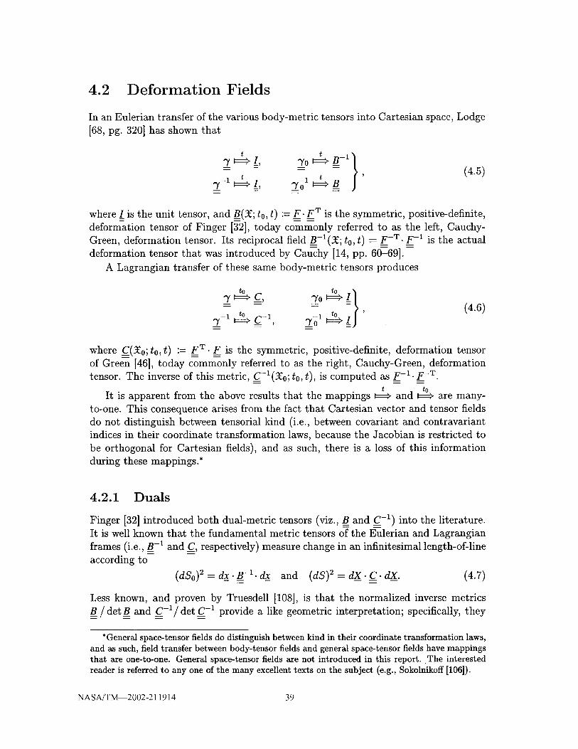
4.2 Deformation Fields

In an Eulerian transfer of the various body-metric tensors into Cartesian space, Lodge

[68, pg. 320] has shown that

t B-I}

_v-° B

____--it t '

(4.5)

where / is the unit tensor, and B(:_; to, t) := F. F w is the symmetric, positive-definite,

deformation tensor of Finger [32], today commonly referred to as the left, Cauchy-

Green, deformation tensor. Its reciprocal field B-1(2¢; to, t) = _K-w. F -1 is the actual

deformation tensor that was introduced by Cauchy [14, pp. 60-69].

A Lagrangian transfer of these same body-metric tensors produces

oc -1, '(4.6)

where C(_0; to, t) := F T. _F. is the symmetric, positive-definite, deformation tensor

of Green [46], today commonly referred to as the right, Cauchy-Green, deformation

tensor. The inverse of this metric, C-1(_0; to, t), is computed as F -1. F -w.t to

It is apparent from the above results that the mappings _=_ and _=_ are many-

to-one. This consequence arises from the fact that Cartesian vector and tensor fields

do not distinguish between tensorial kind (i.e., between covariant and contravariant

indices in their coordinate transformation laws, because the Jacobian is restricted to

be orthogonal for Cartesian fields), and as such, there is a loss of this information

during these mappings.*

4.2.1 Duals

Finger [32] introduced both dual-metric tensors (viz., B and C -1) into the literature.

It is well known that the fundamental metric tensors of the Eulerian and Lagrangian

frames (i.e., B -1 and C, respectively) measure change in an infinitesimal length-of-line

according to

(dSo) 2 = dx . B -_. dx and (dS) 2 = dX. C. dX. (4.7)

Less known, and proven by Truesdell [108], is that the normalized inverse metrics

B/detB and C-_/detC -1 provide a like geometric interpretation; specifically, they

*General space-tensor fields do distinguish between kind in their coordinate transformation laws,

and as such, field transfer between body-tensor fields and general space-tensor fields have mappings

that are one-to-one. General space-tensor fields are not introduced in this report. The interested

reader is referred to any one of the many excellent texts on the subject (e.g., Sokolnikoff [106]).

NASA/T_2002-211914 39

measure change in an infinitesimal area-of-surface according to t

(_X0)2: (dx×&). "- (_x×_) and (_A)_= (_X×__) c-1- det-__ - - detC-1 (dX×_),(4.8a)

or equivalently, according to

C -I(dAoh 2 B ( dA h2=N. -- .N, (4.8b)\dAJ =n-'detB_'n and \dAo] -- detC -1 --

where n and N are the Eulerian and Lagrangian unit-normal vectors to a material

surface, which relate to one-another via the pull-back formula N dAo = dX × dX =

(detF)-lF T. (dx_ x dx_) = (detF)-lF T- ndA. Truesdell [108] closes his little-known

paper with the following insightful theorem.

"The elements of area suffering extremal changes are normal to the prin-

cipal directions of stretch, and the greatest (least) change of area occurs

in the plane normal to the axis of least (greatest) stretch; in fact, if the

principal stretches dS/dSo satisfy _1 _ "_2 _--- )_3 the corresponding ratios

_ __ A "dA/dAo satisfy A2A 3 <_ A1A 3 < I 2.

4.2.2 Rates

In an Eulerian transfer of field, Lodge [68, pp. 321-327] also determined that the

various metric-rates of the body map into Cartesian space as

where

, _-1 o}D_ _ 2D, D"/0 = 0 _ Bt_ =t

D2 -1 _=_ --2D, 02o 1 = O _ = 0

(4.9)

I(L= + L T) (4.10)D(X;t):=is the symmetric rate-of-deformation tensor. The resulting rates, expressed below for

some arbitrary tensor _Y,are defined by

7 A

Y_:=_+LT.j+J.L and _Y:=)-L.J-J.L T, (4.11)

which denote the lower- and upper-convected derivatives, respectively, of Oldroyd [83].

They reduce to Lie derivatives taken with respect to velocity v whenever OJ=/Ot = O.

The common contributing term in these two formulae,

OJ

_)_:: _-_ + (V___J_)•_v, (4.12)

tWe arrived at (3.3) by field transfer. Specifically, we mapped the tensor relations derived byTruesdell [108] from general space into the body, which is a one-to-one operation. Then by executinganother transfer of field, this time mapping the formulae in (3.3) from the body into Cartesian space,which is a many-to-one operation, we arrived at (4.8a).

NASA/T_2002-211914 40

is called the material derivative of _Y, which has a matrix representation of J --

IOJ_c/Ot + (OJrc/OXk)Vk] in the coordinate system C. Here the vector operator _r

denotes the spatial gradient 0/0x.A V

The formulm B = O and B -1 = 0 of (4.9) can be rewritten as quasi-linear evolution

equations for the Finger, B, and Cauchy, B_-1, deformation tensors; specifically,

o

B_°=D.B+B.D and B -1---D.B -1-B -1.D, (4.13)

where the resulting rate, when expressed for an arbitrary tensor Y_,is defined by

j_o:=____ W.J+J.W, (4.14)

and is called the corotational derivative, which was introduced by Zaremba [110] and

is usually credited to Jaumann t, wherein

1w(x;t) := L (4.15)

is the skew-symmetric vorticity tensor. The quasi-linear evolution equation for Finger

deformation in (4.13) lies at the heart of Leonov's [63] viscoelastic theory.V

The corotational _ and lower-convected J deriviatives of any tensor J_ are related

via

_J = _ - D. J- J.D. (4.16a)

Similarly, the corotational _J and upper-convected _J derivatives relate according to

_) = ._ +D-J+ J.D, (4.16b)

where D is the rate-of-deformation tensor. From these identities, one quickly arrives

at the evolution equations (4.13) for B_° and B°-I, given the field transfer results of

(4.9).o 7 o

We point out that rates B(:_; t0, t), B(gC; t0, t), B-1(9C; t0, t) and B-I(:_; t0, t) are alltwo-state tensor fields.

In Eulerian transfers of field where time-based derivatives of absolute, symmetric,

second-rank, body-tensor fields are being mapped into Catesian space, the partial

derivative of a covariant body tensor maps into a lower-convected derivative, while

the partial derivative of a contravariant body tensor maps into an upper-convected

derivative.

$Contrary to numerous citations sprinkled throughout the literature, Jaumann did not publish

the corotational derivative until 1911 [55], where it is given for both vector and tensor fields. An

explicit definition of the corotational derivative does not appear in his book [54] of 1905. Zaremba

[110] was the first to publish the corotational derivative of a tensor field, which he did in 1903.

Nowhere (known to us) did Zeremba publish the corotational derivative of a vector field.

NASA/T_2002-211914 41

In a Lagrangian transfer of field, the body-metric rates map into Cartesian space

according to

D_ _ D_C= 2VT.D-_V_,

D__-1 _ DC-1 = -2 U 1•D. V-T,(4.17)

where DC(Xo;to,t) and DC-l()Co;to, t) are two-state tensor rates, and by DC -1 we

mean D(C -1) and not (DC) -1, the latter of which does not exist, in general.

Fractional order

Because the process of integration commutes with the operation of field transfer [70,

pg. 111], it therefore follows from the preceeding formulae that the Caputo derivative

(1.3) of the metric tensor, D,_(q3; to, t), maps into Cartesian space in a Lagrangian

frame as D,_C(_0; to, t) according to

1 fl 1 O_(t')D*_ - r(1 - a) (t - t') _ -Ot' dt'

D:C= 1__ _i 1 OC(to, t')

-t') a --07--- dt'

= r(1 a) (t 1

2 -t-7 D(t').g,,at'

(4.18a)

D._ (_,t0, t), maps asIn like manner, the Caputo derivative of the dual metric, _ -1 .

D._C -l(xo; to, t) according to

D _ -1 __ 1 £ 1 02-1(#)*Z vii- a) (t --t') _ -_ dt'

D_C_I_ 1_ fl 1 OC-l(t°'t') dt',o *= r(1 c_) (t- t,)_ or,_=_

- £1- r(i 2__) (t -- tt) a g-_l. D(tt). g_T dt',

(4.18b)

where the order of differentiation has been restricted to the range 0 < a < 1. The de-

formation tensors present in these formulae are anchored to state to. These derivatives

have units in time t of order t-%

Given that a < b, the notation F__(a,b)implies Ox(b)/Ox(a), while F-l(a, b)implies

Ox_(a)/Ox(b), thereby establishing notation for a generalized deformation-gradient ten-

sor. Changing the order of the arguments in the deformation gradient is equivalent

to taking its inverse. So we adopt a notation for the deformation gradient wherein

the numeric value of the first argument is always less than that of the second, and

we invert the field, as needed, to satisfy this requirement. Whenever a = to, the

NASA/T_2002-211914 42

shortened notation of Ft, := F(t0, t') is used, and whenever a = to and b -- t, the

accepted notation of F := F(to,t) is used, otherwise F(a,b) is used.

Following in this notation, let B(a,b) := F(a,b). FW(a,b) define a generalized

Finger deformation and let C(a,b) := FW(a,b) • F(a,b) define a generalized Green

deformation. In their arguments, the first state, a, denotes the initial (or reference)

state; whereas, the second state, b, denotes the final (or current) state.

D,_ map intoIn an Eulerian transfer of field, the Caputo derivatives D,n_ and _ -1

Cartesian space according to

1 f" 1 O"),(t')

D_-- r(1- a) ]to (t --t') _ -Or' dt'

_L t 1 OB -l(t',t)

2D.- 1___ /o -- = dt' (4.19a), = r(1 4) (t- at,2 r _ 1

- F(1-a) ]to (t-t') _F-T(t''t)'D(t')'F-l(t''t)dt''

and

ct --1__ 1 /i 1 a_=-l(t')D."/ F(1- a) (t J-t') _ -_i dt'

_r I t I OB_(t', t)

--2D .- f -t = r(i - a) J_o (t - t') _ at, dt' (4.19b)

_ -2 /i 1 F(t', t). D(t'). FT(t ', t) dr',r(i- 4) (t -t,)o- - -at

with D first appearing in a paper written by Drozdov [27] but in a different notation.

Notice that the deformation tensors in the integrands are now anchored to the floating

state t', which is the dummy variable of integration, instead of to the fixed inital state

to. Also notice that the derivatives in the integrands (e.g., OB(t', t)/Ot') are taken at

the reference state of the field (i.e., t') instead of at its current state (viz. t).

The rate-of-deformation tensor, D, has no distinction between tensor kind; how-_L ar

ever, its fractional counterparts have covariant-like, D, and contravariant-like, D,constituents.

The above expressions for the fractional rate-of-deformation tensors can be changed

to anchor to the reference state to by an appropriate application of the chain rule for

differentiation. In doing so, the lower-fractal rate-of-deformation tensor, D(9_; to, t),

of order c_, with 0 < a < i, can be rewritten as

D = r(1 a) (t t') _ FT'D(t')" F_t, dt' • F -1= ..... (4.20a)

1 F-T. (D_.C). F-l,

where the deformation gradients F -T and F -1 can be taken outside the integral

because their state dependence corresponds with the limits of integration. Likewise,

NASA/T_2002-211914 43

ar

the upper-fractal rate-of-deformation tensor, D(X; to, t), can be expressed as

(1 1 )=/_==F" F(1- a) (t-t') _- F_;I"-D(t')'F¢ Tdt' .=F T

= _!F. (D,_C-1) • F T .2 _ _

(4.20b)

From these results it is apparent that the Lagrangian fields D_C_ and D,_C-1 are

the fundamental (most basic) measures for fractional deformation rates in a spatial

formulation in that they are actual Caputo derivatives.

The Lagrangian and Eulerian, fractal, deformation rates of (4.18 & 4.19) are

compatible (in the limit as a goes to 1 from below) with their first-order counterparts,which are: DC = 2 F T. D. F and DC -1 = -2 F -1. D. F -T.

4.3 Field Transfer of Fractional Operators

We are now in a position to map fractional-order derivatives and integrals of any

absolute, symmetric, body-tensor field into Cartesian space in both the Eulerian and

Lagrangian frames of reference.

We begin by considering an arbitrary, symmetric, covariant, body tensor, it, and

an arbitrary, symmetric, contravariant, body tensor, U, whose mappings into Carte-

sian space are known. For purposes of illustration, consider a transfer of covariant

field that is given by

u(V;t) M(X;t),= such that N= FT.M.F, (4.21a)

and consider a transfer of contravariant field that is given by

_=_ G(9_;t), such that H=F-1.G.F -w, (4.21b)_(_;t)= I._ H(:_0;t0, t), = =

where M and G are some arbitrary (but known), symmetric, Eulerian, tensor fields,

with N and H designating their respective, symmetric, Lagrangian, tensor fields.

In these transformations of field, the deformation gradient F_ serves as a Jacobian

of transformation between the Cartesian frames that pulls a known Eulerian field

backwards, out of the Eulerian frame and into the Lagrangian frame.

Lodge [68, pp. 321-327] has shown that the time rate-of-change D of a symmetric

covariant tensor tt maps into Cartesian space as

V

such that DN ---- F T. M. F, (4.22a)

NASA/T_2002-211914 44

while the time rate-of-changeof a symmetriccontravarianttensor__mapsas

A

such that DH = F -1- G. F -T, (4.22b)

V

where M and G are the lower- and upper-convected derivatives defined in (4.11), while

DN ant DH a--re simple first-order derivatives, as their notation suggests. The pull-

bac--k formul--m in (4.22) can also be derived by differentiating the pull-back formulae

of (4.21), as one would expect.

Assuming that the above information is known to us, it is a straightforward matter

to construct the special derivatives of interest.

4.3.1 Derivatives

Here we prove that the Caputo derivative D._ (1.Sa) of a symmetric covariant tensor

tt maps into Cartesian space as

_@ _°tLM' such that D_N_FT.(_M) "F , (4.23a)D,_tt= [_ D._N, -- _ =

while the Caputo derivative of a symmetric contravariant tensor __ maps as

_@ _IG} such that D_H_P-I.(_IG) .F-To (4.23b)D,_= [_:_ D,_H, = = =

The Eulerian tensors _,_LM and _,arG are objective rates of order a defined in (4.26),where notation ,.L, is affiliated with covariant-like fields, while notation ,.r, is affili-

ated with contravariant-like fields. Unlike D,_N and D,_H, which are actual Caputo

derivatives, derivatives _,_LM and _,_rG are not Caputo derivatives, in a strict senseof the definition, which is why they are given a different notation. For this reason, La-

grangian Caputo derivatives are considered the more fundamental of these fractional

rates.

In the derivations that follow, which prove the above mappings, a is restricted to

the range 0 < a < 1.

Pro@ The Caputo derivative of symmetric body-tensor fields map into Cartesian

space in a Lagrangian frame in an intuitive way. For example, for a covariant tensor

tt, its fractional derivative maps as

1 fl 1 Ott(t')D*_tt- r(1 - _) (t - t')_ Ot' dt'

to 1 _[ 1 ON(to,#)D*_N = r(1- a) (t ---t'). -Or' dt',

(4.24a)

NASA/T_2002-211914 45

whereas,for a contravarianttensor_, its fractional derivativemapsas

1 _tl 1 Orl(t')r(1-a) (t--t') _ Ot' dt'

to 1 ftl 1D_H- r(1 - a) (t - t') °

OH(to,t')

Ot Idt I"

(4.24b)

These mappings reproduce standard definitions for Caputo derivatives of spatial fields.

What is noteworthy about these mappings is that the argument list belonging to the

spatial fields being differentiated under the integral sign is (to, t'), designating a fixed

referenced state at to with differentiation under the integrand occurring at the secondstate t'.

The mappings of these same Caputo derivatives (i.e., D_tt and D_r]) from the

body into Cartesian space in an Eulerian frame is a more subtle process. Before

one can proceed, we must know how body-tensor fields from a past state map into

Cartesian space in the present state, which they do according to

tt(t') _ F-T(t', t) •M(t')- F-'(t',t)

__(t') _ F(t',t). G(t'). FT(t', t)(4.25a)

wheret _ t _

tt(t') _:_ M(t') and __(t') _ G(t'). (4.25b)

These transfers of field are distinct from the Eulerian transfers listed in (4.21). Here

the deformation gradient F(t', t) serves as a Jacobian of transformation that pushs-

forward a field that was anchored at some prior time t' into a like field that is now

anchored at present time t.

From the above formulm, it readily follows that the Caputo derivative of a sym-

metric covariant tensor _ maps into Cartesian space in the Eulerian frame as

D_.tt -

t

1 f£ 1r(1 -a) (t - t') _ Ot' dt'

1 _tl 1 O(F-T(t',t).M(t').F-l(t',t))dt':= r(1 - (t - t,)o or, = - =

1 _tl 1= r(1 - a) (t-t') _F-T(t''t)'M(t')'F-l(t''t)dt'

=F-T" ( 1 ftl 1 _ )= r(1 - a) (t --t') _ FT. M(t').Fr dt' • F -1

= F-w. ( l j(i l ON(t°'t') )= r(1 - a) (t --t') _ Ot' dt' • F -1

= F -T. (D_.N). F -1

(4.26a)

NASA/T_2002-211914 46

while the Caputo derivative of a symmetric contravariant tensor _/maps as

t

1-c_) (t - t') _

I=F. D .F T.

= =

o_(r)-- dr'Ot'

_r_ .- r(i - _) (t - t,)a at, - =

_ 1_ f 1_ F(t,,t).__(t,).FT(t,,t)dt,r(1 a) J,0 (t - t,)a - - =

( fo )1 ' __1 F_1.6__(t').F_Tdt' . FT= _" r(1- _) (t- t')o- - = =

( l fi l OH(t°'t') dt') . FT= F. r(1- _) (t ---t,)a -Or, =

(4.26b)

What is noteworthy about these mappings is that the argument list for the spatial

fields being differentiated under the integral sign is (t', t) in the defining integrals,

designating a floating reference state at t'. In the equalities that follow the defining

equality, this reference state is changed from floating (i.e., t') to fixed (viz., t0).R

4.3.2 Integrals

With the above derivations in place, it is a straightforward matter to prove that

the Riemann-Liouville integral ja (1.2) of a symmetric covariant tensor _u maps into

Cartesian space as

{ t_ _atM' such that JaN = F T. (_aLM)'F, (4.27a)za_ JaN, =

while the Riemann-Liouville integral of a symmetric contravariant tensor 7? maps as

2 3a_G' such that Jail =_F -1- (3atG) -F -T. (4.27b)Jar/ jaH, -- _ =_

The Eulerian tensors _aLM and _ar__Gare objective integrals of order c_ defined in

(4.29). Unlike JaN and Ja--H=,which are actual Riemann-Liouville integrals, integrals

_aLM and 3atG are not true Riemann-Liouville integrals, in a strict sense of the deft-

nitio---n, which i--swhy they are given a different notation. For this reason, Lagrangian

Riemann-Liouville integrals are considered the more fundamental of these integrals.

Proof: Like the Caputo derivatives, a Lagrangian map of the Riemann-Liouville

integral for some covariant tensor tt is a straightforward process whose outcome takes

NASA/T_2002-211914 47

the form

J_tt - F(a) (t - t') 1-" tt(t') dt'

to 1 /tl 1JAN-- F(a) (t-t') 1-oN(t°'t')dt''

while for some contravariant tensor rl it becomes

(4.28a)

F(a) (t - t')l-_ _=(t') dt'

to 1 _tl 1_:_ J_H-- F(a) (t-t') 1-_H(t°'t')dt'"

(4.28b)

These mappings reproduce standard definitions for Riemann-Liouville integrals of

spatial fields, and are valid for all c_ > 0.

Using the mappings of (4.25), it follows that the Riemann-Liouville integral of a

symmetric covariant tensor tt maps into Cartesian space in the Eulerian frame as

J_tt - F(a) (t - t') 1-_ tt(t') dt'

I _LM := __

t

= =F •OroN).=F-1,

F(a) (t-t') 1-_F-T(t''t)'M(t')'F-l(t''t)dt'

= F_T. (F__) f_ 1 )= (t - t') 1-_ FT. M(t').Ft, dt' . F -1

(4.29a)

while the Riemann-Liouville integral of a symmetric contravariant tensor rI maps as

t

F(a) (t - t') 1-_ _7(t') dt'

1 _t I 1_rG := F-_ (t-t') 1-_F(t''t) "G(t')'FT(t"t)dt'

( fl ' )= F. (t - t') '-a F}'. G(t'). F} T dt' • F T

=F= (J°H)

(4.29b)

for all a > 0.[]

4.4 Strain Fields

Strain is not a unique concept in finite-deformation analysis. Here we present two,

Cartesian, strain fields that relate to changes in length-of-line. The first pertains to a

separation between material points, while the second pertains to a separation between

NASA/T_2002-211914 48

material planes. A third measure of strain accounts for changes in the volume of a

material point. These concepts are presented in both their Eulerian and Lagrangian

constructs.

As it turns out, the strain fields used in the constitutive theories of Chp. 5 are

different from the classic strain fields that are discussed in this chapter. Be that as

it may, the strain fields presented in this chapter are of historical significance, and

seeing how they arrive from field transfer should aid the reader's understanding of

how the spatial strain fields of Chp. 5 are arrived at.

4.4.1 Covariant-Like

The covariant strain tensor of (3.8) maps into spatial strain fields that are well known.

In particular, in an Eulerian transfer of field,

= 1 _ _ := l(t- B=-I), (4.30a):=

where A(:E; to, t) is the Almansi [2] strain tensor, while in a Lagrangian transfer of

field,

1 __ 1 (C -/) (4.30b)E:= ,

where _E(:E0; to, t) is the popular Green [46] strain tensor.The-Almansi and Green strains are symmetric fields that measure a change in the

distance-of-separation between a pair of neighboring material points.

Rates

From (4.22a), the time rate-of-change of strain _e_maps into Cartesian space as

D _ A = D,1 = = (4.31)De__= _ DE= ½ DC= FT. D" F,_

V

where A is the lower-convected rate of Almansi strain, and DE is the Green strainV

rate, both of which are well-known results. Formula A_= D can be rewritten in terms

of the corotational derivative via (4.16a) as

&=D-D.A-A.D, (4.32)

thereby producing a quasi-linear equation for the evolution of A in terms of its

Zaremba-Jaumann derivative.

Fractional order:

into Cartesian space according to (4.23a) as

The fractal, covariant, strain-rate tensor, DT_e, of (3.11) maps

_L

_A = D,aL

1Da. C=F T D.FD_E= 5 = "

__ 1 FT. D(t,) . Ft, dt ,,f:o 1(t-t') _ __ __ __

(4.33)

NASA/T_2002-211914 49

where _tA_ is the lower-fractal, Almansi, strain-rate tensor, and D___ is the fractional,

Green, strain-rate tensor, both of order _ wherein _ is restricted to the interval0<_<I.

4.4.2 Contravariant-Like

The contravariant strain tensor of (3.12) maps into Cartesian space in an Eulerianframe as

l/_-I _ l(B-/), (4.34a)

where Z_(X; to, t) is a strain tensor that was introduced by Signorini [104], and whose

appearance in the literature is scarce. A Lagrangian transfer of this same body field

yeilds

1(_-1 _ 1(/_ C-1), (4.34b)

where Y(_0; to, t) is a strain tensor whose origin is unknown to us, and that we shallsimply refer to as a Lagrangian strain tensor.

The Signorini and Lagrangian strains are symmetric fields that measure a change

in the height-of-separation between a pair of neighboring material planes that are

non-intersecting.

Rates

From (4.22b), the time rate-of-change of strain 4 maps into Cartesian space as

1 =D,D¢==-_Dv -1= [_ DY---_IDC-1---__F -1.D-F -T,

(4.35)

where _ is the upper-convected rate of Signorini strain, and DY is the Lagrangian

strain-rate. Because of (4.16b), formula _Z = _D can be rewritten in terms of the

corotational derivative as

Z_° = D +n. Z+Z.D, (4.36)

thereby producing a quasi-linear equation for the evolution of Z in terms of its coro-tational derivative.

Fractional order:

sor, D,__, of (3.14) maps into Cartesian space as

According to (4.23b), the fractal, contravariant, strain-rate ten-

A. = D,1 a-1 1 a-1=F-1. (4.37)D_. ¢ = -i D,'7 D_Y -_ _ === D,C /_-F -T

__ 1 tr(1-.) fro (t-t,1)" F-_I. _D(t') "=F-_T dt',

where _,_IZ is the upper-fractal strain-rate tensor of Signorini, and D,_Y is the upper-

eth, fractional, Lagrangian, strain-rate tensor, both of order a wherein 0 < a < 1.

NASA/T_2002-211914 50

4.4.3 Dilational

Using the preceeding results of this chapter, it is also a straightforward matter to map

the dilatation A(t0, t) of (3.15) from a body formulation into a spatial formulation,

thereby producing

= ln(det F) (4.38a)A = ln(det (3,ol. 3,) 1/2) _:_ A = ln((det B) 1/2)

in an Eulerian setting, and

o(dot( o ln(Idet = ln(det F) (4.38b)

in a Lagrangian setting. There is no distinction between the Eulerian and Lagrangian

descriptions for dilatation, as expected, because dilatation is an absolute scalar field,

and is therefore independent of the Jacobian of transformation between these twoframes.

Rates

A consequence of the above transfers for strain rate is that the time rate-of-change of

dilatation (3.16) maps from the body into Cartesian space in an Eulerian frame as

1 _=_ DA = tr D,DA = 3 tr D_ _-- (4.39a)

and it maps into Cartesian space in a Lagrangian frame as

DA= ½trD3, t=_z Dz_= 1 C -1" DC=trD. (4.39b)3= = =

Again, there is no distinction between configurations because the transferred field isan absolute scalar.

Fractional order: The fractal rate of dilatation, D,_A, can be computed as

1 f0 t 1D_A-- F(1- a) (t-t') _(trD)(t')dt'' (4.40)

which follows straight away from (4.39), or equivalently, from a field transfer of (3.17).

This equation applies to both spatial frames of reference.

Conservation of mass

From the results of (4.38 & 4.39) it follows that the conservation of mass, whose rate

form is

1 _ Dlnt_ =DIn t) = -3 tr D_, = -trD, (4.41a)

integrates toOo dV

Q -- dVo - det F, (4.415)

in accordance with (3.15).

NASA/T_2002-211914 51

4.5 Stress Fields

In an Eulerian transfer of field, Lodge [68, pp. 327-328] has shown that the body-stress

tensor K maps into Cartesian space as

t_:_ T, (4.42a)

where __T(:_;t) is the Cauchy [14, pp. 42-56] stress tensor. The equation for deviatoric

stress (3.19) therefore maps to Eulerian space as

1 t _ltrTjp := -g tr _ _:v p :=

(4.42b)

where -_Tis the deviatoric stress associated with hydrostatic pressure p in Cartesian

analysis.

In a Lagrangian transfer of field, the body stress maps into Cartesian space as

to

oo _ P, _r _ P*, (4.42c)-_-___ _

where P(9_0;t0, t) := _ F -1- T. F -T is commonly referred to as the second, Piola-

Kirchhoff, stress tensor, named after the independent works of Piola [85] and Kirchhoff

[58]. Tensor P*(i_0;t0, t) := F -1- T. F -T is a Lagrangian stress tensor.§ Both fieldsare symmetric, two-state, stress tensors. The deviatoric stress and the hydrostatic

pressure of (3.19) therefore map into the Lagrangian frame as

_ 1_°'_:_P:=P+_-pC-1 and -_-p_',_-p:=-gP'C, (4.42d)

both of which are widely used definitions.

4.5.1 Conservation Laws

The physical law that impacts stress is the conservation of momentum.

Balance of linear momentum

This law yeilds a vector formula, called the stress equations of motion, that in an

Eulerian frame is given by

Qa_= V. T + Qf, (4.43a)

where V_. 7" is the divergence of stress, with a matrix representation of IOT,.k/OXk] in

coordinate system C, and where vectors _a and f denote acceleration and body force,

respectively.

§In the literature, the notation _* is often used to denote the first, Piola-Kirchhoff, stress tensor,

F -1. T, which is not symmetric. The stress tensor that we call P* is seldom used. For us, tensor

P_* -- _F-1- T. F -T is a natural choice, since it arises directly from a field transfer of the body-stress

tensor __.

NASA/T_2002-211914 52

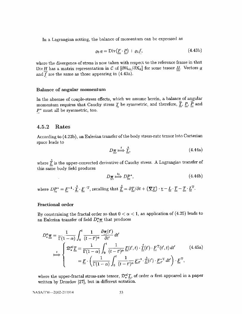
In a Lagrangian setting, the balance of momentum can be expressed as

00a_ = Div(F-P) + _0f_, (4.43b)

where the divergence of stress is now taken with respect to the reference frame in that

DivH has a matrix representation in C of HOHrk/OXk_ for some tensor H. Vectors _a_

and f-are the same as those appearing in (4.43a).

Balance of angular momentum

In the absense of couple-stress effects, which we assume herein, a balance of angular

momentum requires that Cauchy stress _T be symmetric, and therefore, _, P, _ and

P* must all be symmetric, too.

4.5.2 Rates

According to (4.22b), an Eulerian transfer of the body stress-rate tensor into Cartesian

space leads tot a

D_- _=_ T, (4.44a)

A

where T is the upper-convected derivative of Cauchy stress. A Lagrangian transfer of

this same body field produces

Dn" _:_ DP*, (4.44b)

A

where DP* = _-1. _. F-T, recalling that T = OT/Ot + (_'__fT).v - L. T- T. L T.

Fractional order

By constraining the fractal order so that 0 < a < 1, an application of (4.25) leads to

an Eulerian transfer of field D_ that produces

1 for 1 O_(t')D*_-V(1-a) (t - t') _ Ot' dr'

{ _r T = 1 t 1

= r(1- a) fo (t-t')

( 1 for 1 _ )F" i,_( 1 __ 0_) (t -- tt) a F_I" T(tt)" F_T dt' • F T,

(4.45a)

where the upper-fractal stress-rate tensor, _,_rT, of order a first appeared in a paper

written by Drozdov [27], but in different notation.

NASA/T_2002-211914 53

A Lagrangiantransferof the samefield leadsto

I/0 D*_ - r(m -- _)

D._P -t0

1 O_(t') dt'(t- t,)_ at'

1 [t 1 OP*(to, t') dt'

r(1 - a) Y0 (t - t'p Ot'1 ft 1

r(1 - _) ]o (t - t,p F=_l"T(t') . F=__ dr',

(4.45b)

where D_P* = F -1- _,_tT. F -T, which is compatible with its first-order counterpart

DP* = F -1- ]_-F -T in the limit as a goes to I from below.

NASA/T_2002-211914 54

Chapter 5

Constitutive Theories

Continuum theories are presented in this chapter that are suitable for elastic and

viscoelastic materials. Both compressible and incompressible constructions are dis-

cussed. Each theoretical structure is reduced to cases of material isotropy and trans-

verse isotropy. The resulting theories are mapped into Cartesian space in the Eulerian

and Lagrangian frames of reference for use when solving boundary-value problems.

Tangent moduli are also derived so these theories can be implemented into finite

elements. Material functions are assigned to these theories in Chps. 7-??, thereby

producing material models that can then be compared against experimental data.

5.1 Integrity Bases

The theory of invariants [107] is well developed as it pertains to our needs. In the

case of a single tensor--say, A--having a matrix representation A in some admissible

coordinate system affiliated with the underlying manifold, there exists an integrity

basis that is comprised of three, irreducible, moment invariants:

trA, trA 2, trA 3. (5.1a)

This set constitutes an admissible, isotropic, integrity basis for any single, symmetric,

3 × 3 matrix A. One advantage of using an integrity basis is that scalar fields can

replace tensor fields as arguments in state functions. Another advantage is that an

integrity basis leads to tensorial structure in a potential-based theory without having

to introduce any ad hoc assumptions.

None of the above three invariants can be expressed solely in terms of the other

two; they are orthogonal to one another. Even so, this basis is not unique. The

Cayley-Hamilton theorem--A 3 - (tr A)A 2 -t- 1 ((tr A) 2- tr A2)A- (det A)][ = 0, with

l((trA)2- trA 2) and detA--permits an exchange of the cubicinvariants: tr A, _

moment (i.e., trA 3) with the determinant (viz., detA - ½{trA 3 - trA[(trA) 2 -

3 tr A2}) when assigning an integrity basis. Furthermore, if matrix A is non-singular

(i.e., detA _ 0), then another application of the Cayley-Hamilton theorem allows

the quadratic moment, trA 2, to be replaced by the moment of its inverse, trA -1.

It is accepted practice to make use of both of these exchanges when assigning an

NASA/T_2002-211914 55

integrity basisfor isotropic elasticity; specifically,trA, trA -1, and detA areoftenemployedbecausethey leadto practiclemodels,eventhough they do not consititutean irreducibleset.

For the caseof two distinct matrices--say,A and B--then in addition to thoseinvariantsthat involvea singlematrix only, onemust alsoconsiderthe coupledtraces

tr AB, tr A2B, tr AB 2, tr A2B 2, (5.1b)

making a total of ten invariants that now comprise this irreducible integrity basis.

When preference is given to one coordinate line above all other coordinate lines,

then the resulting integrity basis is said to be transverse isotropic. Let vector a be

a unit vector that is tangent to this coordinate line. Because there is no directional

preference along a coordinate line, the integrity basis must be even in a, and as

such, vector a can be represented by the symmetric dyadic matrix B := a ® a with

components B --= laraC_, wherein ® denotes the outer product between two vectors.

Because a is a unit vector, it follows that a _ a = (a e a) 2 = (a ® a) 3 .... , and it

also follows that tra ® a = I, tr A. (a ® a) = a. A. a, tr A 2. (a ® a) -- a. A 2. a, etc.

Consequently, of the ten invariants in (5.1a & 5.1b) only five are independent; they

are:

trA, ira 2, trA 3, a.A-a, a-A 2.a, (5.1c)

which define the irreducible, transversely isotropic, integrity basis for matrix A.

The intellectual process of selecting an integrity basis will lead to a constitutive

theory. This is not a straightforward process because, although the irreducible in-

tegrity basis is unique, there are numerous, other, orthogonal, integrity bases that are

also admissible and therefore may be considered. Mathematics alone is incapable of

selecting an integrity basis; physics must also be addressed. Once a theory is in hand,

the process of assigning/deriving a potential function appropriate for the selected in-

tegrity basis will produce a constitutive model. Only when such a model is available

can the challenging process of characterization and (hopefully) verification against

experimental data begin to take place. In physics, one cannot prove a theory/model

to be correct. One can only, perhaps, disprove it, or more importantly, establish its

domain of applicability.

5.2 Elasticity

Here we consider a mass element _ of density _(_; t) in a state of stress _(_; t) that

is undergoing an infinitesimal change in shape of d_(_3;t) := _(_; t+dt) -V_(_; t)

over an increment in time of dt. This induces a differential change in the work done,

dW(_; t), on the mass element (including the energetic contribution due to its change

in kinetic energy) that is quantified by the formula [70, pp. 194-195]

1

dW = 26 _ d% (5.2)

From thermostatics, given an arbitrary reversible process, V --+ _/+ d_/, the incre-

ment of work done on a mass element minus the change in its kinetic energy (herein

NASA/T_2002-211914 56

denotedasdW) equates with a change in the internal energy of the mass element.

For an isothermal reversible process, the increment dW equates with a change in the

Helmholtz free-energy of the mass element.

Equation (5.2) leads to a potential-based constitutive equation for elasticity,

_--_ 0_ OIn (5.3)oo 0_3 _ 200 0I,_ 0_'T _ = 2_OoO_ n=X --

which implies that (5.2) is an expression of the chain rule. The potential func-

tion representing elastic strain-energy density, W(_; 0, t) = _I_(11,12,---, IN: 9; 0, t),

has arguments that make up an integrity basis comprised of N independent invari-

ants I,(_o,_,XI,X2,...,XM-2: _;0, t), n = 1,2,...,N, obtained from M sepa-

rate tensor fields: the metric tensors _0 and "7 along with M - 2 material tensors

X m, m -- I, 2,..., M - 2. The tensor gradient a_I_/0__ must be symmetric (i.e.,

0_I]/0_ ----½10_13/0yrc + cO_2IJ/0ycrl in every body-coordinate system B: _ --+ _) in or-

der for it to satisfy the conservation of angular momentum. All anisotropic attributes,

when present, are manifest through the gradient 0_I_/0__, which has units of stress

on mass density. Unlike classical elasticity, there need not be a fourth-rank modulus

tensor that assigns anisotropic characteristics in the theory of finite-strain elasticity;

instead, the integrity basis introduces them through its gradients.

When elasticity is described by a potential function then the material model is

called hyper-elastic, and although there is no mathematical proof for its existence,

Leonov [66] has provided physical proof for its necessity (there is no know proof of

sufficiency): non-potential, finite-strain, elastic (so called hypo-elastic) constitutive

relations can be constructed that create energy from nothing (i.e., they can operate

as perpetual motion machines); hyper-elastic constitutive relations cannot be con-

structed to violate thermodynamics in this way. This justifies referring to (5.3) as

the fundamental constitutive equation governing elasticity.

Theromostatics places loose constraints on what are admissible functional forms

for the potential function _. This is an important topic in constitutive modeling,

but it lies outside the scope of this report.

5.3 Viscoelasticity

One can 'fluidize' the above, elastic, constitutive laws, moving them beyond the realm

of reversible thermostatics and into the domain of irreversible thermodynamics, by

introducing a memory function that bestows a loss of remembrance onto past states

[18]. The contributions that can be recollected from each past state are then summed

over a loading history. Stress and strain are taken to be causal functions of time

during this integration, and as such, are zero valued for all times prior to time t = 0.

However, loading histories may be discontinuous at time t = 0, as will be the case in

creep and stress-relaxation experiments.

The well-known constitutive equation for linear viscoelasticity, restricted to in-

finitesimal strains and rotations, can be written as the following Volterra integral

NASA/T_2002-211914 57

equation [47],

t OEk_(O, t') dt'.Tij(t) =Giy(t)Eke(O,O +) + Gijke(t- t') Ot'+

After an integration by parts, this expression becomes

_0 tTij(t) =Gijkl(O)Ekt(O,t)-- Mijkl(t--t')Eke(O,t')dt',

or equivalently, using the additive and anti-symmetric property of infinitesimal strain

(i.e., Ekt(O,t) = Ekt(O,t') + Ekdt',t), t' e [0, t]), it can also be written as

f0 tTij(t) = Gijkt(t)Ekl(O,t) + Mijk_(t-- t')E_t(t',t)dt',

where Tij = Tji are the symmetric components of stress, Ekl = g_k are the symmetric

components of infinitesimal strain, Gijkt = Gjikl = Gijtk are the symmetric compo-

nents of a relaxation modulus, and Mi#ke(t -- t') := OG{jkt(t -- t')/Ot' are the symmetric

components of a memory modulus. Memory fades if IMijkt(t2)l < IMijke(tl)l for all

t2 > tl > 0. In classic viscoelasticity, the fourth-rank material functions Gijkl and

Mijk_ account for material anisotropy, when present.The first of the three formulations listed above requires the strain to be continuous

and differentiable over time. The second and third formulations are less restrictive in

that they only require strain to be continuous over time. The last two formulations

differ in the moduli of their elastic terms, and they also differ in the states that define

strain in their viscoelastic (integral) terms. It is the third expression of these three

equivalent expressions that we choose to analytically continue from the infinitesimal

into the finite.

In all three of these classic formulations, strain is the controlled variable to which

stress responds. Because the theory is linear, it can also be written so that stress is the

control variable to which strain responds. But in our end application (finite elements),

displacements are assigned to which forces respond, which motivates selecting strainfor the cause and stress for the effect.

Using classical viscoelasticity as our guide, and adopting the hypothesis of Kaye

[56] and Bernstein et al. [7] (which they applied to viscoelastic liquids) wherein strain

is replaced by the gradient of strain energy, as in elasticity theory, we therefore con-

sider a class of K-BKZ - like viscoelastic solids that obey the constitutive hypothesis

Qo 9Jt.(t O_ OI.(t',t)-_-__ = 260 _ qS.(t) OI_ O'y(t) + - t') OI_ O'_,(t) dt' , (5.4)

and as such, produce a work increment (5.2) of

N( O_ Oi_(O,t) fot O_20 0I_(t',t) )dW = E ¢3_(t) OI. O_'(t) + 9:;t.(t- t') Oil O'),(t) dt' " d')'(t),

NASA/T_2002-211914 58

wherethe viscoelasticstrain-energydensity W(_; t', t) = _]3(I1,/2,..., IN" °43;t', t)

with invariants I,(_t,, _', X1, X2,-.., XM-2: _3; t t, t), n = 1, 2,..., N, is constrained

such that 0_(_; t, t)/O_ = 0 (there can be no strain when the two states defining

strain are one in the same), and where _'t, := _(_; t') with t' C [0, t].

The n th relaxation function, ¢3n(t- t'), which is positive and dimensionless, along

with its associated memory function, _n(t -t') := 0¢5_(t -t')/Ot', which is positive,

has units of reciprocal time, and is monotone decreasing, do not specify anisotropic

characteristics, when present, which is different from classical viscoelasticity. This

task is relegated to the gradient of strain energy, 0_/0_, which has units of stress on

mass density. The fact that the memory functions, _, are positive and monotonic,

and that the state of integration, t', replaces the initial state, t = 0, as the reference

state in the invariants of the integrand, are both in agreement with the hypothesis of

a fading memory [18, 19].

It is because the memory function convolves with a first-order derivative (i.e.,

strain 0_/0_), whereas the relaxation function convolves with a second-order deriva-

tive (viz., strain rate 02_!lJ/Ot 0_,), that motivated our selection of the K-BKZ - like

constitutive structure presented in (5.4) as the phenomenological foundatation for our

theory of viscoelastic solids.

This type of construction (based on an elastic strain-energy density) is particularly

attractive for modeling solids that are predominantly elastic with some viscoelastic

attributes, like the materials of interest to us (viz., elastomers and soft biological

tissues).

Equation (5.4), which is applicable for viscoelastic solids, is slightly different from

the construct that one would use for viscoelastic fluids [71], which is

N f_ ,, O_a30I_(t', t)II = -r/s D_7 -1 + 200 Z j_ ffJtn(t - t )oi_ O_'(t) dr', tr D__7-1 = 0,

n--_- i O0

wherein rls represents solvent viscosity. Fluids are usually considered to be incom-

pressible, and as such, the extra stress II replaces the body stress ,r in its construction.

Furthermore, the viscous response of the solvent present in a viscoelastic fluid replaces

the elastic response that is present in a viscoelastic solid. Finally, the lower limit of

integration is moved from zero to minus infinity in the fluid theory, because fluids do

not have a unique reference state.

In contrast with the classic formulae of viscoelasticity, the constitutive theories

presented in this chapter place no restrictions on the extent of either strain or rotation.

Thermodynamics places loose constraints on what are admissible functional forms

for the strain-energy density _r, relaxation _5_, and memory 9Yt_ functions. Like

elasticity, this is an important topic, but it lies outside the scope of this report.

5.4 Tangent Operator

Commercial finite-element packages often require a user to supply a tangent operator

(or modulus) for user-defined constitutive equations so that its solver can construct

NASA/T_2002-211914 59

an optimal stiffness matrix. Even though finite-element programs do not employ body

tensors, it is still advantageous for us to construct this fourth-rank tensor in the body,

and to then map it into the required frame of Cartesian space for later use in finite

element analysis.

The tangent operator _(q3; 0, t) is a fourth-rank contravariant tensor defined by

_E:=2 0'e_],[_ sothat d(_)=_(ld_=_E'dE, (5.5)-- 03" _ - _ =

where _e is the strain tensor of (3.8). This operator has symmetries (in a body-

coordinate system B) of _/jkl __ _jike = _jlk = _jitk because stress _ and strain _e

are symmetric fields. In component form, (5.5) reads as _jke = 20(e_ 7tij)/Oykl.

For the elastic constitutive equation of (5.3), the tangent modulus becomes

N (Of$1J 02I. N_l o2fllJ OIm OI._ (5.6a) 0 03+ 0±m0zoo3"®b-4/'-- n=l __ __ = : :

which mandates an additional symmetry of _°°°°_jke _ _klij. The tensor outer product

r/® r/ has components xliJ_]ke in coodrinate system 13. In most material models,

includingthose of this report, 02fCO/OIm OIn = 0 for all m _ n, thereby simplifyingthe above modulus so that it becomes

N (0_ 02fn 02_ OI. OI_) (5.6b)=4QoE _n 03" 03" +-0I_ 03' ®_/"

In keeping with the assumption that there are no cross-coupling terms arising between

the various invariants in the functions selected to represent strain-energy density, it

follows that

N Q O_ 02fn fo t ,.02YO O2in dt '= 4Qo E _5.(t) 0[. 03" 03" + 9Jt.(t - t ) _ O'y 03"-- rill

_ . 02f_ OIn OIn fot 02_ Ofn OIn )

(5.7)

for the viscoelastic constitutive equation of (5.4). Some care is required here becuase

I_ = I_(O,t) in the elastic terms; whereas, I_ = I_(t',t) in viscoelastic (integral)terms.

5.4.1 Stability

For an elastic or viscoelastic solid to be stable requires that it be Hadamard stable,

and as such, satisfies a condition of strong ellipticity where it becomes necessary andsufficient that

_iJklxiYjXky e > O, V X__, y. (5.8a)

NASA/T_2002-211914 60

A more useful condition (in accordance with 5.5), which is necessary but not sufficient,is that

de: E" de= d(-_) -d__e> 0, V d__e. (5.8b)

This is a thermodynamic condition for stability, the so-called Drucker [28] stability

postulate, which is not a physical law.

The necessary and sufficient conditions for strong ellipticity are extremely complex

and awkward to verify for any given model. It is for this reason that attempts have

been made to obtain sufficient conditions for strong ellipticity that are of ample

generality to be useful to the model developer. Of note are the works of Renardy

[92], Leonov [651 and Kwon and Cho [61], all of which address viscoelastic liquids.

Dissipative stability, pertinent for a stability analysis of viscoelastic liquids [65],

has no role to play in the stability analysis of viscoelastic solids.

5.5 Isotropic Elasticity

An isotropic elastic solid can be formulated in terms of two, mixed, tensor fields

when being described by body-tensor fields; in particular, consider A := _o15 and

B := _-:_i0,* where one field is the inverse of the other. The conservation of mass,

det(v-l-_0) = (0/00) 2 > 0, guarentees that V__-:'_0 is non-singular, and consequently,

invertible (and therefore, _o:" _ is non-singular and invertible, too). As such, only

three of the ten possible invariants in (5.1a & 5.1b) are independent. In what follows,

we will postulate the existance of an integrity basis that is comprised of sums of like

invariants taken from these two deformation tensors, and in doing so, we average their

characteristics.

From a mechanics perspective, there is no reason to choose the deformation vari-

able _o:" _ over deformation variable _-1. V_0, or vice versa. However, from a physics

perspective, the molecular network theory of rubber elasticity (i.e., the neo-Hookean

solid [53]) produces a constitutive equation described soley in terms of _o1._ [72].

This contrasts with the popular phenomenological model of Mooney [80] that uti-

lizes both deformation fields in its description, and whose rigorous derivation from

statistical mechanics continues to elude researchers.

Rivlin [93, 94, 95, 96, 97, 98] and his students, Saunders [99] and Gent [39, 40, 41],

were amoung the first to derive constitutive equations from an integrity basis for finite-

strain isotropic elasticity, and to perform multi-dimensional experiments to seek out

admissible functional forms for the strain-energy density. Reiner [91] was the first to

*As is the norm in general tensor analysis, the trace of a tensor field (in this case, 7_o: and

_'_o)is achieved through a contraction with the metric 7__:= 7__(_,t), t > 0, or, when appropriate,

its inverse 7_-1 := _-:(_, t). It is because of this fact that gradients (i.e., c9_tJ/O"l.=.)can arise froma strain-energy density W = _(I_;i = 1, 2,..., N) that may otherwise be considered as resultingfrom non-conservative sources, (e.g., one can introduce D__ as a state variable). This is one veryimportant reason why we prefer using body-tensor fields for the purpose of deriving constitutivetheories.

NASA/T_2002-211914 61

actually deriveconstitutive equationsfrom an integrity basis.Todaythey arecalledReinerfluids.

Flory [34]proposeda multiplicative decompositionof the deformationfield (defin-ing _ := (det_)-I/3_ so that det_ = I) as a wayto uncoupledeviatoricand hydro-static responses, which has certain advantages from a computational perspective [105].

We choose not to make such a decomposition in this body of work because the in-

variants we have chosen have gradients that are strain fields, not deformation fields

as is typically the case, and therefore, it is not certain if the added complexity of

introducing such a decomposition is warrented at this time.

Adding respective invariants from the two deformation tensors, _,oI-_ , and _,-i. To,

each anchored to a different state, averages the effect of reference state that is tacitly

held by these two measures for deformation and leads us to consider the following set

of invariants as our integrity basis:

) ,:: /det( o

(5.9a)

whose gradients, t

(5.9b)

tHere we have used the following results to derive the gradients OIn/O"¢ and 02I_,/O"y O"i:

0"y-- = fi [] _, with components in B of OYkl 1 L_.i£J i j

and

O_ -1 i)ykt

_ __-1[] ,l-i, with components in B of 07ij_ _(¢_

noting that I_oX._l= I_o_lI_l- i_ll•

NASA/T_2002-211914 62

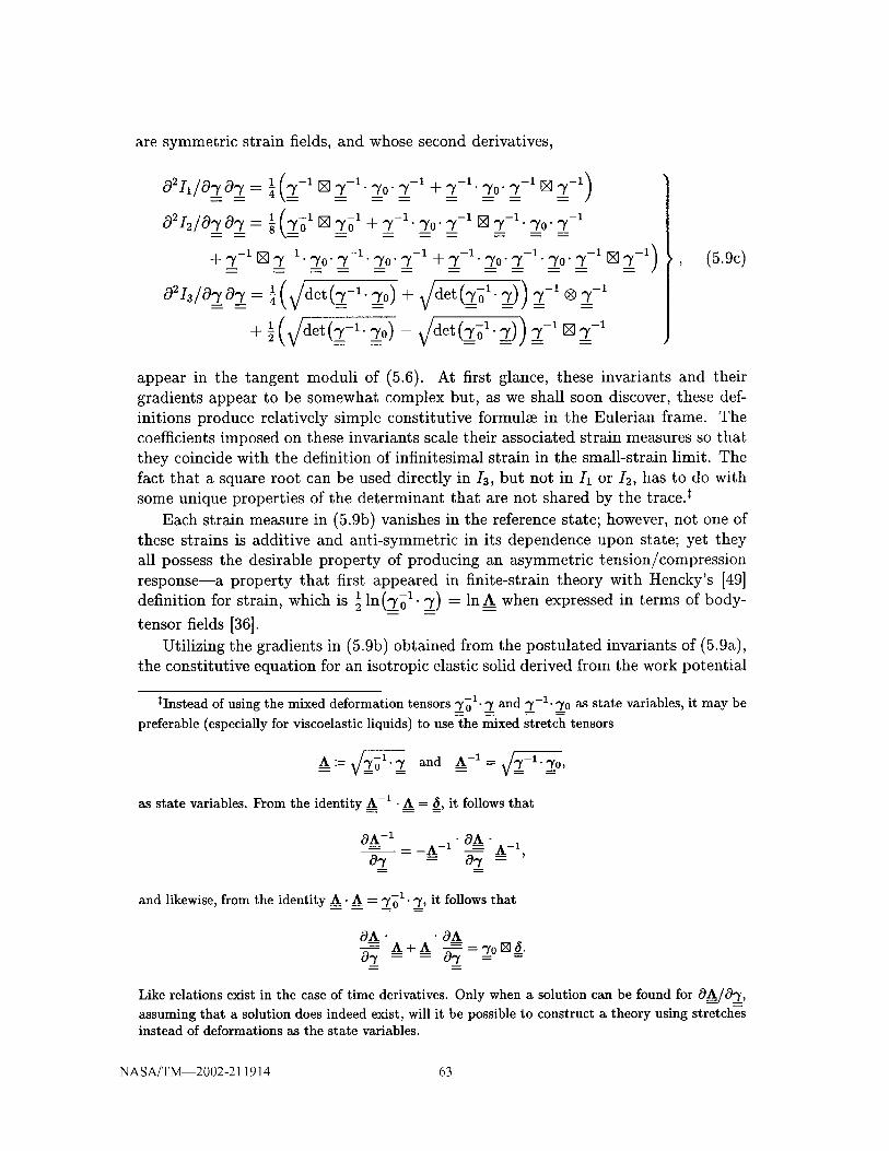
are symmetric strain fields, and whose second derivatives,

o2h/o o == I -1 I+ .7-1 [] ,7-1..70" .7-1. "To" .7-1 + .7.),-1..70" .7-1. "70" .7-1 [] 7=-1) ['

0213/0.70.7= 4 (v/det(_-l" Z°)+ Idet(z°l" _--)) Z-1 ® Z-1 /

+ ! det .7-1..7o - det .7o 1- .7 .7-1 [].7-1I_ I_ _/)_ _ J

, (5.9c)

appear in the tangent moduli of (5.6). At first glance, these invariants and their

gradients appear to be somewhat complex but, as we shall soon discover, these def-

initions produce relatively simple constitutive formulae in the Eulerian frame. The

coefficients imposed on these invariants scale their associated strain measures so that

they coincide with the definition of infinitesimal strain in the small-strain limit. The

fact that a square root can be used directly in/3, but not in/1 or/2, has to do with

some unique properties of the determinant that are not shared by the trace, t

Each strain measure in (5.9b) vanishes in the reference state; however, not one of

these strains is additive and anti-symmetric in its dependence upon state; yet they

all possess the desirable property of producing an asymmetric tension/compression

response--a property that first appeared in finite-strain theory with Hencky's [49]

1 ln(_o 1 7) = lnA when expressed in terms of body-definition for strain, which is _ • =

tensor fields [36].

Utilizing the gradients in (5.9b) obtained from the postulated invariants of (5.9a),

the constitutive equation for an isotropic elastic solid derived from the work potential

*Instead of using the mixed deformation tensors 7 -I- 7 and _,-I._o _ _ "To as state variables, it may be

preferable (especially for viscoelastic liquids) to use the mixed stretch tensors

_--A:= ____1._/_ = and =A-I=_= = ,

as state variables. From the identity A -1 • A_ -- 5, it follows that

OA -i • OA".A-I _ A-l,

07 ---- 07 ----

and likewise, from the identity A- A = 7_01. 7_, it follows that

0A- • 0A

-02 A+A _ =7oN5.==

Like relations exist in the case of time derivatives. Only when a solution can be found for 0A/0%

assuming that a solution does indeed exist, will it be possible to construct a theory using stretchesinstead of deformations as the state variables.

NASA/T_2002-211914 63

in (5.2) has a stress response of

( 1 <__= 2_0 _,1 _ _o - _- __° 7=

1( ._._o I _0. _0-_ -1)+ _,2 _ 7=01 _ 2_-1. _-1.

+_,3_1 (_/det (_o 1 • _=)- v/det (_=-1" "70)) 0'-1)= = ,

(5.10a)

whose trace defines a state of hydrostatic pressure (3.19b)

-¢ P = -g Oo 1_ _/ o " _ - " o

+ _2 _(_ol.-y.-yo_:-_=-7=-_.-y0.-_-l.7=0)

+ 3!_/,3 l(_/det(7=ol" _)- _/det(_-l. _0))),

(5.10b)

that for materials whose bulk moduli are many times more stiff than their shear

moduli becomes§

ido ( -i (5.1Oc)

Here _,i := 0_I/(0, t)/OIi, i = 1, 2, 3, are three material functions that can, at most,

depend upon the three scalar invariants Ii(0, t), I2(O,t) and I3(0, t). The invariants

in (5.9a) are defined as sums between like invariants taken from the two stretch

tensors, _o 1. _ and _-1. _0- Cureously, hydrostatic pressure p is described in terms

of differences taken between these same, fundamental, stretch invariants.

For the special case of an (ideally) incompressible material, the above theoretical

structure reduces to

(II= 2_o0 _,1 _ "_0 = _[ 0''y-1 1 __7=-1. ,.y--1.

(5.10d)

which is similar to setting _,3 = 0. Tensor II (= p 3, -1 + _) is the extra-stress of

(3.20a), with p being a Lagrange multiplier that forces a constraint for incompress-

ibility, det _' = det _'0.

The tensorial nature of (5.10) is fixed. Its structure is a direct consequence of

the chosen integrity basis listed in (5.9). Only the three scalar functions _,i are

adjustable. Their specification will turn this theory for elasticity into a material

model, which is the primary topic of Chps. 7-??.

§It is for this reason that we do not find it necessary to decouple strain into separate hydrostatic

and deviatoric parts.

NASA/T_2002-211914 64

5.5.1 Field transfer

Using the results of Chp. 4, it is a straightforward process to map this theory for

isotropic elasticity from the body manifold where it was derived into Cartesian space

where it will be used to solve boundary-value problems. The main results from these

mappings are outlined below.

Lagrangian frame

When the time of field transfer coincides with initial time t = 0, then the resulting

Cartesian fields are referenced to the Lagrangian (or material) configuration. In this

frame of reference, the isotropic elastic invariants of (5.9a) are computed as

l(tr C + trC-1) }

Ii = _ =

/2=16(1( trC2)= + (tr C-'= )) , (5.11)

Ia = v/de-_=C + v/dee C-1 = det F + det F-1

where C (= F T. F) is the symmetric deformation tensor of Green (4.6), often called

the righ--t, Cauchy-Green, deformation tensor, in which tensor F (= Ox_/OX) denotes

the deformation gradient defined in (4.2).

An isotropic elastic solid whose invariants are so defined has a stress response

(mapped from Eqn. 5.10a) of

( 1 1 (det F - get F -1 ) (5.12&)P= 2LOo _,l,l(t-- g-2) ___ _,2 _(C- g-a) ____,3 _ : = ) C-l= ,

with P being the second, Piola-Kirchhoff, stress tensor defined in (4.42c). In the

incompressible case, (5.10c) maps to space as the constitutive formula

p* + _aC-1 = 200 (_,1 1(I - C-2) + _,2 _ (C - C-3)), (5.12b)

subject to a constraint for incompressibility, det F = 1. Tensor _P* (= _ P) represents

the Lagrangian stress tensor of (4.42c) that, in the incompressible limit, is equivalent

to the second Piola-Kirchhoff stress ___becuase 0 = Q0.

Eulerian frame

When the time of field transfer coincides with current time t, then the resulting fields

in Cartesian space are referenced to the Eulerian (or spatial) configuration. In this

frame of reference, the isotropic elastic invariants of (5.9a) are computed as

}= +

/3 = d_ + _r_t B-1 = det F q- det F -1

(5.13)

NASA/T_2002-211914 65

where B (= F. F T) is the symmetric deformation tensor of Finger (4.5), often called

the left, Cauchy-Green, deformation tensor. Because the trace of a matrix product

is independent of the order in which the product is taken, these Eulerian invariants

equal their Lagrangian counterparts, which is why they are called invariants.

An isotropic elastic solid whose invariants are defined by (5.13) has a stress re-

sponse (mapped from Eqn. 5.10a) of

--= ( -- detF-1)I)12 1 (detF- (5.14a)_or 2_0_,1¼(B- B-1)+ _,2 _(B B-2)+ _,3

with __Tdenoting the Cauchy stress defined in (4A2a). For the incompressible case

(from a mapping of 5.10c), the stress response of (5.14a) reduces to an extra-stress

response of

( )),+ _t= 2_0_,1¼(B- B-1)+ _,2 _(B2- B-2where the Lagrange multiplier p forces a constraint for incompressiblity, det F = 1.

Special care must be taken when implementing this constitutive equation (in fact,

when implementing any nearly incompressible material model) into finite elements

so as to avoid possible ill-conditioning of the stiffness matrix leading to a potential

locking of the mesh caused by an overconstrained displacement field.

It is here, in the Eulerian frame, that the full simplicity of our constitutive theory

for isotropic elasticity (derived from the integrity basis of 5.9a) is most apparent.

Equation (5.12a) can be pushed forward into the Eulerian frame producing (5.14a)

by contracting (5.12a) with F from the left and F T from the right. Conversely, (5.14a)

can be pulled backward into the Lagrangian frame producing (5.12a) by contract-

ing (5.14a) with F -1 from the left and F -T from the right. These are appropriate

push-forward/pull-back mappings for contravariant-like tensor fields. Because these

mappings apply to T and P*, and also to _ ___Tand P, it is sufficient to obtain a single

transfer of field from the body into Cartesian space (hereafter, we will provide map-

pings into the Eulerian frame) from which the corresponding formulation in the other

(viz., Lagrangian) frame can then be readily acquired by applying the appropriate

(i.e., pull-back) mapping between these two Cartesian configurations.

Generalized strain fields:

generalized strain fields of the type

=E(n) := !{Bn4n_= - B-n)' n • _, (5.15a)

with dilatation being approximated by the scalar measure

e := ½(detF- detF-1), (5.15b)

where instances n = 1 and n = 2 are the strain fields present in (5.14) so that ¶

0---qT:0: 2_o0/_, ,1:_(1) -[- _23- E(2),__ + _,3 e/__), (5.16a)

¶Another constitutive theory that may prove useful is

_-T = 2Qo(aE (V2) + bE (1) + ce_/_),

The elastic theory presented above is constructed with

NASA/T_2002-211914 66

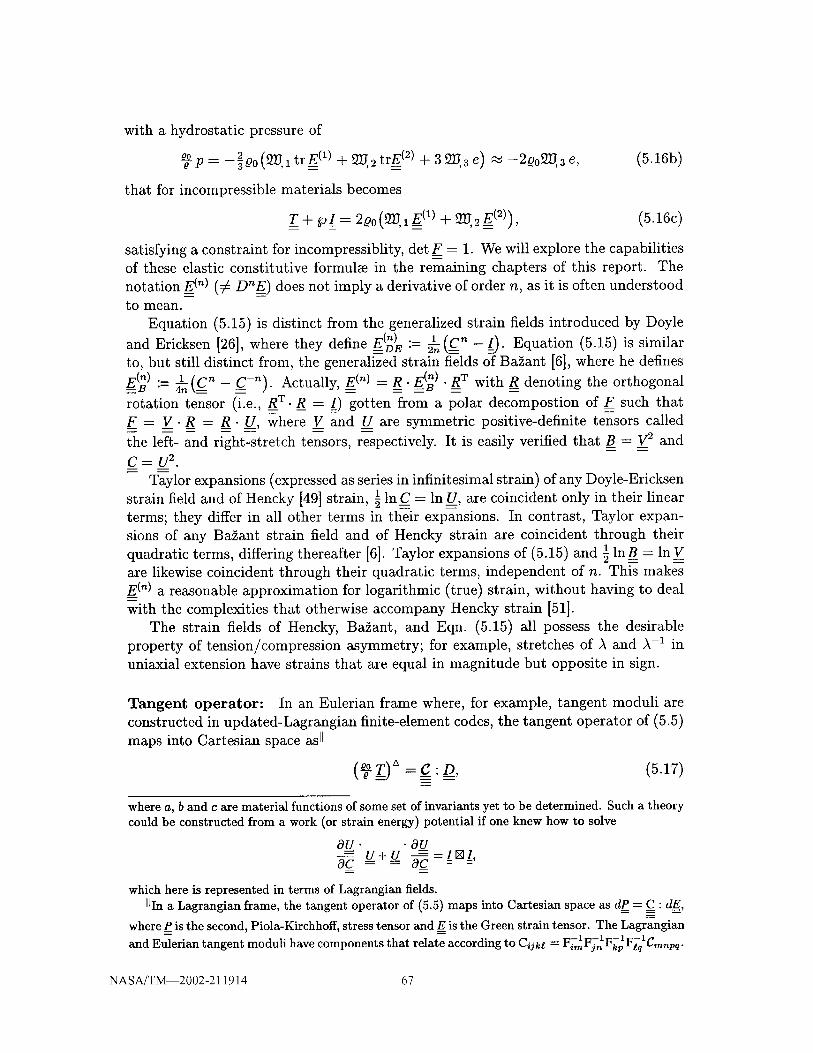
with a hydrostatic pressure of

_p 2 (_, trE(m) +_,2trE(2) + 3_,ae) _ -200_,3e, (5.16b)

that for incompressible materials becomes

-_- gO/= 2L00(_,1E(1) -_- _2 E(2)), (5.16c)

satisfying a constraint for incompressiblity, det F = 1. We will explore the capabilities

of these elastic constitutive formulm in the remaining chapters of this report. The

notation E__(n) (5 DEE) does not imply a derivative of order n, as it is often understoodto mean.

Equation (5.15) is distinct from the generalized strain fields introduced by Doyle

and Ericksen [26], where they define E_(_) "- l(cn - I). Equation (5.15) is similar__ "-- 2n \_

to, but still distinct from, the generalized strain fields of Ba2ant [6], where he defines

E--_)_ "-'- l(Cnd___-- - C-n) Actually, =E(n) = _R" E(_ ). =RT with =Rdenoting the orthogonal

rotation tensor (i.e., RT-R = /) gotten from a polar decompostion of F such that

_F = V. R = R. U, where _V and U are symmetric positive-definite tensors called

the left- and right-stretch tensors, respectively. It is easily verified that B = _V2 and

C= U 2.

-- T_ylor expansions (expressed as series in infinitesimal strain) of any Doyle-Ericksen

i In C = In U, are coincident only in their linearstrain field and of Hencky [49] strain, _ = =

terms; they differ in all other terms in their expansions. In contrast, Taylor expan-

sions of any Ba_ant strain field and of Hencky strain are coincident through their1 In B = In Vquadratic terms, differing thereafter [6]. Taylor expansions of (5.15) and _ = =

are likewise coincident through their quadratic terms, independent of n. This makes

E_(_) a reasonable approximation for logarithmic (true) strain, without having to deal

with the complexities that otherwise accompany Hencky strain [51].

The strain fields of Hencky, Ba_ant, and Eqn. (5.15) all possess the desirable

property of tension/compression asymmetry; for example, stretches of A and A-1 in

uniaxial extension have strains that are equal in magnitude but opposite in sign.

Tangent operator: In an Eulerian frame where, for example, tangent moduli are

constructed in updated-Lagrangian finite-element codes, the tangent operator of (5.5)

maps into Cartesian space as II

(_T) A =Z'D, (5.17)

where a, b and c are material functions of some set of invariants yet to be determined. Such a theorycould be constructed from a work (or strain energy) potential if one knew how to solve

Ou • • Ou

-Oc u+u =INI,==

which here is represented in terms of Lagrangian fields.

"In a Lagrangian frame, the tangent operator of (5.5) maps into Cartesian space as dP = C : dE,

where P_P_is the second, Piola-Kirchhoff, stress tensor and _E is the Green strain tensor. The Lagrangian

F-1F-1F-_F-l(,and Eulerian tangent moduli have components that relate according to Cijke = im jr* kp tq ,-'rnnpq.

NASA/T_2002-211914 67

where D is the rate-of-deformation tensor defined in (4.9), T is the upper-convected

rate of Cauchy stress given in (4.44a), and where the fourth-rank tensor G__is the

Eulerian tangent operator obtained through the field transfer _ _ C_.

The tangent operator for the isotropic elastic solid of (5.14) is given by

c-4 0( 1 1)÷(.___1 11+_ I((B=[]B=)+ (n=-i[]_-1)+ (t[]_-2)+ (_-2_t)) +_,22(_(_)®_(2))

))+_,3e(/[]t) + (_,3_h+_,33e_)(/®/ ,(5.18)

where 2IJ, i = Of21J/OIi and 21_,ij = 0221J/OIiOIj, i,j = 1, 2,3, and where tensor prod-

ucts M [] N and M ® N have matrix representations of M [] N = _(MikNj_l + Mi_Njk)]

and M ® N = _MijNkl] in the coordinate system C. This tangent modulus was

obtained by substituting (5.9b & 5.9c) into (5.6b) and mapping the resultant into

Cartesian space. Not all of the terms in (5.18) will be contributing in any given

model; furthermore, additional terms will be required if the function representing

strain-energy density has a cross-coupling of ImI_, m _ n, in its definition.

5.6 Isotropic Viscoelasticity

With a general structure for isotropic elasticity in place, it is a straightforward process

to extend this structure to a theory for isotropic viscoelasticity using the constructs

of (5.4), which is based upon the K-BKZ [7, 56] hypothesis. As in the case of isotropic

elasticity, the stress response has three constituent parts, one related to each invariant,

that combine to quantify the total state of stress according to

T_----2Q00l(t)_,l(0, t)_ ")'o _-- _'Y0''Y

+ _l(t-t')_,l(tt, t) l('yt-,1-_-l"_/__t,'_'-l)dt'

+ ¢_2(t)_2(0, t)_ (3'or" 7" _'o t - 3'-1" 70" 7-1" 70" _'-1)

1 --1 ,._--1 ,_--1. dt'+ _2(t-t')_,2(t',t)g 7=t,1.7__.7_¢-= "Tt," 7__t"7=-_

+ ¢_3(t)_,3(0, t)½ (v/det(_ol" "y)- v/det(_-l" ")'0))_ -1

1 det(_=,1-_)_ v/det(___._,)) _t'_-1 ,+ _YY_3(t-t')_,3(t',t)_ =

(5.19)

where the invariants of (5.9a), adjusted for time interval [t', t], lead to constitutive

formulae that satisfy the required constraint of O_I_(t, t)/O__ = O whenever t' = t.

NASA/T_2002-211914 68

There are three, independent,scalar-valued,relaxation functions _i, i = 1, 2, 3,

in this consitutive equation whose associated memory functions are computed as

9YQ(t - t') := 0¢5_(t - t')/Ot'. The three _5i are dimensionless, positive and bounded.

Their memory functions _7_i(t - #) have dimensions of reciprocal time, they can

possess a weak singularity at t t = t, they must be positive, and they must decrease

monotonically with a sufficiently rapid rate of decay towards zero as t goes to infinity,

all in accordance with the hypothesis of a fading memory [18, 19]. The fact that the

memory function can be weakly singular at t' = t is offset by the required constraint

that 02B(t', t)/O_ = 0 whenever t' = t, so the integrand as a whole remains regular

over the entire interval of integration.

One possible simplifying assumption that can be considered is to set the relaxation

moduli q51 and 62 equal to one another, indicating that shear flow is governed by a

single relaxation mechanism, independent of the order of strain.


Using the results of Chp. 4 and, in particular, Eqn. (4.25), the stress response of the

isotropic viscoelastic solid listed in (5.19) has an Eulerian description of

( /0t°° T = 2_0 el(t)_,l(O,t)EE_(1)(O,t)-k - 9Yq(t-t')_,l(t',t)E(1)(t',t)dt '

/o+02(t)_2(o,t)g(_)(o,t)+ _2(t-t')_2(t',t)E=(2)(t',t)dt'

f )+ 05a(t)f_,a(O,t)e(O,t)I + gJla(t- t')f_J,a(t',t)e(#,t)dt' I= ,

(5.20a)

that, for materials whose bulk modulus is much greater than its shear modulus,

produces a hydrostatic pressure that (approximately) satisfies

( /0 )-_p = -2Qo ¢53(t)_,3(O,t)e(O,t)+ ff23(t-t')_,a(t',t)e(t',t)dt'. (5.205)

For incompressible materials, this constitutive description simplifies to

( /0'T+ _9/= 200 ¢51(t)_,l(O,t)E(1)(O,t)+ 9Ytl(t-t')_,l(t',t)_(1)(t',t) dt'

I/ )+05_(t)_2(O,t)E(21(O,t)+ _2(t-t')_2(_',t)_21(t',t)dt ' ,

(5.20c)subject to a constraint for incompressiblity: either detF ---- i or trD_ = 0. Here

F(t',t) := Ox__(t)/Ox(t') = F(0,t)- F-l(0, t ') and B=(t',t) := F__(t',t). FT(t',t) so that

E(_)(t',t) = l(Bn(t',t)-B-_(t',t)) and e(t',t)= l(detF(t',t)-detF-l(t',t)). This

is the theory for isotropic viscoelasticity that we employ for solving boundary-value

problems.

NASA/T_2002-211914 69

Tangent operator

The tangent operator (5.7) is composed of two parts for each invariant--an elastic

part and a viscoelastic part--whose sum produces the overall tangent modulus for

the isotropic viscoelastic solid of (5.20); specifically,

c_ = c__ + c v, (5.21a)

such that upon substituting (5.9b &; 5.9c) into (5.7), and then mapping the resultant

into Cartesian space, one obtains an elastic part that when expressed in the Eulerian

frame is given by

C__¢ = 4_Oo I_l(t) _,1_ / [_ B-l) -I- (B-1 [_ t -F _ 11 (E__(1) @ E(1)

+_(_)(__((_:__)+(_-__ _)+(_ _)+(__)(5.21b)

(_ _(_[] _i_)+ (_ 1i3+_ ¢_)(_®_))),\

+ _3(t)

and a corresponding viscoelastic part that is given by

C v= 4_Oo(for 9:Itl(t-t')_,l(t',t) ¼((INB-l(t',t))+ (B-l(tt,t)[_I))dt !

/o'+ gJh(t--t')f_,11(t',t)(E(1)(t',t)®EO)(t',t))dt '

+ _2(t-t')f_,2(t',t)l((B__(t',t)NB(t',t))+(B=-l(t',t)NB=-l(t',t))

+ (/NS_-_(t',t))+ (B=-_(t',t) Nl))dt ' (5.21c)

fo+ _2(t-t')f_,22(t',t)(E__(2)(t',t)®E__(2)(t',t))dt'

+ _YQ(t-t')_,3(t',t)\e INI +_ 3_, =

£ )+ _3(t-t')_3a(t',t)e2(t',t)(I®I__)dt ' ,

with additional terms required whenever the function representing strain-energy den-

sity has a cross-coupled dependence between its invariants.

5.7 Transversely Isotropic Elasticity

We now address materials composed of a single family of fibers, or showing a single

preferred orientation. Let the contravariant vector __0 := _(_, 0) be a tangent to this

NASA/T_2002-211914 70

material line of anisotropy at a particle _ in the reference state of time t = 0, and

let this vector have unit length in this state so that it satisfies

c_0.70"g0 = i. (5.22a)

At current time t, the fibers along this material line will have stretched by an amount

A according to

A2 = C_o. 7 .C_o. (5.22b)

Any material obeying such a symmetry property is called transversely isotropic, be-

cause the transverse material plane (defined by a normal vector that is coaxial with

the covariant vector 7o" go) remains isotropic. Virtually all biological tissues are at

least transversely isotropic. Many are orthotropic, and therefore exhibit two prefer-

ential directions, but we will not address this or any other higher level of anisotropy

in this report.

In order to construct an elastic theory for transverse isotropy, in accordance with

(5.1c), we need to introduce two additional invariants to the three isotropic invariants

that already exist and which are defined in (5.9). The two additional invariants that

we propose to use are defined by

1 ( ) }/4 := _CI_0" 2 +20. =7---1" 20 " _---0 , (5.23a)

---1 _o. + •whose gradients are anisotropic strain measures given by

oz,/oz: 1((__o®__o/-z-_.zo•(__o®__o/.zo.=_-_) }0±5/02= 1((go ®go)-2-201 -2-1.2o • (go®go)-2o-7-1-_o-V= -1 ,

+7ol-7.= =(__o®_o) - 7-1. 7o-7-1- 70-_ = = (go ®go) -7o-2 -1)(5.23b)

and whose second-order derivatives, present in the tangent moduli, are

o2q/o7o7 = ¼(2-1 [] 2-1.2o. (go ®go) •7o. v-1

+2-1.20. (go®go). 7o.7-1[]2-1)

o_q/o7o7= 1((go ®go)[]201+201[] (go®go)+2-1[]2-1.20.(go®go) .70-7-1.70.7-1+ 2-1. 20. (go ®go) -20.2 -1 [] 2 -1. 2o. 2 -1 • (5.23c)

+ 7_-1" 70" (go ® C_o)•7_0"7_-1" 70" 7 -1 [] 7 -_

+ 7 -1 [] 7 -1" 70" ____-1. ,.)tO. (_---0 ® _____0) " 70" 7 -1

-4- 7 -1" 70" _.._.--1 [] _._.--1. 70" (gl_O ® ¢3_0) "_.0" _..__--1

+ 7--1" 70" 7--1" 20 " (O____0®C_0)"70"7--1[_<]7 -1)

NASA/T_2002-211914 71

Collectively,the five invariantsof (5.9a& 5.23a)constitute an admissibleintegritybasisfor transverselyisotropicmaterials.**Gradients011/c9_ and 014/0__ are strains

of first order; whereas, gradients 012/0_ and 015/0_ are strains of second order.

From these five invariants, one arrives at the constitutive equation for an elastic

solid with transverse isotropy derived from the work potential in (5.3); it has a stress

response of

i( <y__=20o 1_ _o - _o"

+ _ _(_o_._. _o_- _-_._o.<. __o._-_)

+ _,3 ½ (v/det(___ol" _Y)- v/det(_-l" ___o))___ -1

+_,4_((__o®__o)-_-_.zo.(__o®__o).__o._-1)+_,__ ((__o®__o)._-_o_-_-_-_o.(__o®__o)-_o._-_-_o._-1

+_o1._ •(__o®__o)-_-1-_o-<-_o-(__o®__o)-_o-<)).

(5.24)

There is an apparent symmetry in tensorial structure between the contravariant fields:

-701 and c_0 ® _0, and between the covariant fields: __0 and __o" (_0 @ _0) • __0.


Before one can proceed with a mapping of this constitutive equation from the body

into Cartesian space, it is necessary to determine how the unit vector _a0 of (5.22)

maps into space. In a Lagrangian transfer of field, let the Lagrangian unit vector a_0

be defined by the field transfer

o }____o_ _ao

to

_0"_0" _0 = 1 _=> a_0- a__0= 1

__o'_ _o A2 to =A2• = _=> g_o. C • _a_o

(5.25a)

**It was our desire to construct meaningful, anisotropic, finite-strain measures that led us tochoose invariants that are themselves a sum of like invariants constructed from fields with opposing

variance (e.g., one constituent invariant arises from the contravariant form of a state variable, whilethe other arises from the covariant form for that same state variable). Constructing meaningful,isotropic, strain measures is not a difficult task; there are many admissible choices. However, thereare few admissible choices to select from when attempting to construct meaningful, anisotropic,strain measures. Equation (5.23b) presents one such pair of acceptable strain fields.

NASA/T_2002-211914 72

so that in an Eulerian transfer of field one gets

t2o _:::_A a_

B-1 A-2_o.,To._o = 1 _=_ a • -_a_=

20"q"C_o=A 2 t_=:_ a . a = l, (5.25b)

and therefore a = A-1F- a_0, or equivalently, £0 = A F_-I" a_• Material curves defined

by the trajectory of a0 are indicative of fiber direction. After a deformation F, these

fibers have a new direction of a, and they have stretched by a factor of A. Vectors a_0

and a are the same vector fields that were utilized by Spencer [107, pg. 13].

To the invariants of (5.11 or 5.13) we add (gotten by a field transfer of Eqn. 5.23a)

14 =I (C-q-C -1) _ao and 15=lJ_£0-(g2-i-C-2)-ao, (5.26)_ao"

which are different in form from the invariants used by Spencer: _ao.__C-_aoand a_o-_C2._ao.

Affiliated with the invariants of (5.26) are the two, anisotropic, Eulerian, strain fields

A(1)::4A(2) ((-_ -) : - -)=_)) ) }

!A2 a®a -B -1.(aQa .B -1

:=1o ((- - _- = -±A 2 (a®a).B+B.(a@a (5.27a)

-- B -1. ((a@a)-B -1 -I-B -1- (a@a)).B -1)

which result from a transfer of the fields in (5.23b). Recalling that

A2 = a0. C. a_o and a = A-l_F._a_0, (5.27b)

allows these anisotropic strain fields to be recast as

_(_)= _((_. ao)®(_-a0)- (E_-a0)®(E_"ao)) }A=(_)= _ ((_.._o)®(B_.__._-0)+ (_.g-._o)®(g"_-o) . (5.27c)

_ (_=-T.ao) ®(_._-1.ET. a0)_ (8=-1.E_.._0)®(g-_'-_o))These are still Eulerian strain fields, it is just that they are represented in terms of

the material vector ao instead of its spatial variant a. In the deformed state, vector

_F- a0 is tangent to the material line of anisotropy, while vector F -T. a0 is normal to

t-he plane of isotropy, as illustrated in Fig. 5.1, and these vectors need not be coaxial.

A compressible, transversely isotropic, elastic solid whose invariants are so defined

has a stress response (mapped from Eqn. 5.24) of

{_T=2eo(_,lE(1)+_-E(2)+_,3eI+_,4A(1)+_,sA(2))_ = ,.,.= = _ , (5.28a)

that in the incompressible case becomes

T + go/= 2Qo (_, 1E (1) +_-E (2) + _,4A_(1) + !_, 5 A(2)) (5.28b)

where the Lagrange multiplier p forces a constraint for incompressiblity, det F = 1.

These are the formulations for transverse-isotropic elasticity that we investigate in

the remaining chapters of this report.

NASA/T_2002-211914 73

Tangent, _.-1 F _ Fib/_r jNormal, Xv-T" a0 Direction

_ Materiall Plane _

Figure 5.1: Kinematics of a transverse-isotropic material.

Tangent operator

To the isotropic, elastic, tangent operator listed in (5.18), one must add an anisotropic,

elastic, tangent operator (obtained from substituting Eqns. 5.23b & 5.23c into Eqn. 5.6,

and then mapping the resultant into Cartesian space), which is given by

/

C a _--- 4kO0/1_,4z_2(t[_ (_m_-1" (a@a)-B -1) --_ (_-1. (a@a).B-1) [_t)

+ 1__,5 a_(_=[](a®a) + (a®a)[]g

-I-/[_ (_-1. ((a®a) "B-1 -I- _-1. (a®a)). _-1)

-t- (B -1. ((a®a)._-1___ B-1. (a®n))-B -1) _]t

(cq-_,44 (A (1) ®A (1,) q-_,55 (A (2, ®A(2))) .

(5.29)

Again, additional components will need to be included into this expression if there

exists a cross-product dependence between the invariants in the function representing

strain-energy density that is being considered.

NASA/T_2002-211914 74

5.8 Transversely Isotropic Viscoelasticity

In accordance with our elastic theory for tansverse isotropy (5.24), an application

of the K-BKZ - like constitutive hypothesis for viscoelasticity (5.4) produces a vis-

coelastic constitutive relation governing the stress response of a transversely isotropic

material that has five constituent parts, one associated with each invariant, and is

given by

I (%;1 -- ,._--I. •__:2_o ¢_l(t)_(ot)_ : o'o0,-1)

_0 _ --I __ "_t'"+ 9Jh(t-t'l_,l(t',t)_("/,,l _ _-1 . ,7-1)dt,

+ _2(t)_I_,2(0, t)_ (0'o1" "y "'Yo 1 -- _-1" 0_0" 0'-1" _0" _ -1)

/0 )i -i -i _ _-i. .y-i dt'+ _2(t-t')_,2(t',t)g t' ""Y'"_t' = "It" "_t""_ -1

2t- _)3(t)_,3(O,t)1 (v/det(%01" 2 - Cdet(_/-1. _=0))_ -1

+ _ootO23(t_t,)_,3(t,,t)½(v/det(v_t,l.v__)_ v/det(o,_i.O,r))d t, %-1

+_(t) _ _(o,t) _((__o®__o)- _=-1._=o.(_o®__o).2o._=-_)

£+ gYq(t-t')fJ2J,4(t',t)l((_e®_r)-2-1"2t,'(_t,®_t')'Tt"'Y-1) dr'

"4- e5(t ) _l, 5(O,t) i ((CI_ 0 ® _.-_-0)" _" _t01 -- %--1. %0" (_-._-0® _-_-0) "'_0" ,_f--l.,.)tO.,_t--1

-_-%O1"% " (____0®____0) -- %--1" _'0" _y--1" %0" (O_0®C_0)"20"% -1)

+ gJts(t-t')fgOs(t',t)

× 1 ((___,®___,)•__._j_- Z-_--2,.(m,®_,) .-.--<--_,,--<

+_=_z (-_"®-_")__-1.._,,..<.__,,.(__,,®__,,)..,,,..<)@,\

(5.30)which contains isotropic viscoelasticity (5.19) as a special case.

A possible simplifying assumption that one may choose to consider would be to

set @1 = @2 and @4 = @5, thereby implying that relaxation behavior does not

discriminate between the first- and second-order strain fields, yet it does discern a

difference in the relaxation behaviors along the strong direction and in the plane of

isotropy.

Another simplifying assumption to consider, which is applicable for at least some

biological tissues [101], is that _bl = _b4 and @2 = @5, with the implication being

that relaxation behavior does not vary between the strong direction and the plane

of isotropy, even though the elastic response can possess a strong anisotropy; yet,

NASA/T_2002-211914 75

unless_1 = _2, too, (and therefore_51= _52= _54= _5) the material candiscerna differencebetweenthe relaxation behaviorsdue to first- and second-orderstraineffects.

A moreusefulassumptionwouldbe to eliminatethehigher-orderinvariants/2andI5 that introduce nonlinear capabilities, provided that experiments, or the boundary-

value problems to be solved, justify making such a simplification.


The vector of anisotropy in the reference state of integration, __t,, maps into Cartesian

space in this floating frame of reference as follows,

_t, _ at,

t r

c_t,-_t,-c_t,=l_at,.at, =1

t _

_t"V=" _t' = _2(t',t) _ at," C(t',t).-at, = )_2(t',t) j

(5.31a)

and consequently, it maps into the Eulerian frame as

c_t, _ A(t',t)_q

t

_t,.V=t,._t, = 1 _ a._B-l(t',t).-a = A-2(t',t) ,

o_t," __" _t, = A2(t _,t) _::_at a=l

(5.31b)

where A(t', t) denotes the stretch along the fiber axis over the time interval [t', t].

Furthermore, the anisotropic strain fields are given by

n(1)(t,,t) : 1/_2(t,,t)((a@-a) _ (B-l(t,,t). (a@-a).B-l(t',t)))

- B-l(t',t) " ((Ca@a)'B-l(t ',t)) -_- (B-l(t',t) • (a_@a))).B-l(t',t))

(532a)wherein

_2(t',t) =-at,-C(t',t)-at, and -a= A-l(t',t)F(t',t)._at,, (5.32b)

with

A2(0, t') =_a_0.C(0, t')"-a0 yielding _at, = A-l(0, t')F(0, t ') .a0, (5.32c)

which generalize the formulae of (5.27).

NASA/T_2002-211914 76

The stress response of the transversely isotropic viscoelastic solid given in (5.30)

has an Eulerian description of

( f0_°° T = 200 ¢51(t)fYO, l(O,t)E(1)(O,t)+ ffYq(t-t')_,l(t',t)E(1)(t',t)dt '

+052(t)f_2(O,t)E=(Z)(O,t)+ gYC2(t-t')f_,2(t',t)E=(2)(t',t)dt'

+053(t)f_a(O,t)e(O,t)I+ _3(t-t')f_,3(t',t)e(t',t)dt'I

+ 054(t) f_,4(O,t)A(_l(O,t) + gJh(t- t') f2_,4(t',t)A(_l(t',t)dt '

/o_ )+05(t)f_,_(O,t)A(_l(O,t)+ _5(t-t')f_,5(t',t)A(2_(t',t)dt ' ,

(5.33a)

that, for an incompressible material, reduces to

( f0_T+ _/= 2cOo _)l(t)_,l(O,t)E(1)(O,t)+ 9YQ(t-t')_,l(t',t)E(1)(t',t)dt '

fo'+02(t)f_,2(O,t)E(2l(O,t)+ _2(t-t')f2O,2(t',t)E(2_(t',t)dt'

fo_+e4(t)f_,4(O,t)A(_)(O,t)+ 9)h(t-t')_,4(t',t)A=(_)(t',t)dt'

fo_ )+055(t)_,5(O,t)A(2_(O,t)+ _(t-t')_,5(t',t)A(2)(t',t)dt ' ,

(5.33b)

subject to a constraint for incompressiblity: either detF = 1 or trD = 0. These

are the formulations for transverse isotropic viscoelasticity that we exercise in the

remaining chapters of this report.

Tangent operator

To the two parts already listed for the isotropic, viscoelastic, tangent operator in

(5.21), two additional parts must be considered to account for transverse isotropy,

such that

C__= C_e + C ea + C_v + Cv., (5.34a)

NASA/T_2002-211914 77

where the isotropic components C e and C_ are found in (5.21b & 5.21c), and where

the anisotropic components are given by

/ / _

ce°=4e0 _(t) _ t[](_-l.(__®.) _-1)+(_-1.(._®__) _-l)[]t

+ _,44 (A(1) (_ 4 (1)))

_ 5 _ (B [] (__®a) + (__®__)[]B+ _s(t)

+ 8=-_ [] (_-_. (__®__)._-') + (_-1. (._®_.)-_-_) []=8-1

+'-_('---_((-"®"-)"---_+'P (_-®-"))_-9

"_- (B-X- ((a(_a).B-1 -}-B-l. (a(_a)) .B-I) [_/)

+ ®_(t)_(A (_)®a(_))),(5.34b)

and

(/0 (eva = 4_o 9YQ(t-t')_4(t',t)¼A2(t',t) IN(B-l(t',t).(a®a_).B-l(t',t))

+ (B-_(t',t). (__®__)-B-l(t', t)) []1)dr'

f/+ 9Jt4(t-t')f_lJ,44(t',t)(A_(1)(t',t)®A(1)(t',t))dt '

l (+ 9Y_s(t-t')f_,s(t',t)_A2(t',t) B(t', t) N (a_ ® a) + (a_e _a) N B=(t', t)

+ B=-l(t', t) [] (B-l(t', t) • (a N _a). B-l(t', t))

+ (B=-l(t',t). (a_® a)-B__-l(t', t)) [] B__-l(t', t)

-{- t [] (B-l(t"t)" ((_ @ _a). B-l(t',t) --{- B-l(t',t) • (a ® a_)). B-l(t',t))

-_- (B-l(t', t) • ((a ®a). B-l(t',t)+ B-l(t', t) • (a® G_)). B-l(t',t)) NI)dt'

// )+ _s(t-t')f_,55(t',t)(A_(2)(t',t)®A(2)(t',t))dt' ,

(s.s4c)with additional terms required if the function representing strain-energy density hap-

pens to depend on cross products between its invariants.

NASA/T_2002-211914 78

Chapter 6

Finite-Strain Experiments

Although many characterization experiments are 1D in concept, they are 3D in reality

and often require 3D analysis, even for the simplest of deformation histories, espe-

cially when finite strains are being considered. We restrict our discussion to those

experiments whose stress and strain fields remain spatially uniform (homogeneous)

throughout the specimen. Furthermore, deformations are assumed to be controlled to

which forces are measured as reactions, while temperature is held constant. This re-

striction of controlling deformations and measuring forces, although imposed herein,

is by no means a requirement of characterization experiments. Shear-free extensions

and simple shearing are the deformations considered.

Deformation rates and strain rates are known because they are controlled. Force

rates and stress rates, on the other hand, are usually not measured. Whenever stress

rates are present in a constitutive equation, be they of integer or fractional order,

a system of differential equations ensues that needs to be integrated to arrive at a

predicted stress that can then be contrasted with the observed stress. This requires

that stress rates be handled different than strain rates for purposes of characterization.

6.1 Shear-Free Extensions

A deformation is said to be shear free if there exists a convected coordinate system

(e.g., B: _ -+ _) that is always orthogonal [70, pg. 81]. In this class of experiments,

a uniform material element in the shape of a unit cube is deformed into a rectangular

parallelepiped causing tractions to set up on the various material faces, dependent

upon boundary conditions, as illustrated in Fig. 6.1. These experiments are techno-

logically important for solids because of their relative ease of execution. They are,

however, extremely difficult to execute on fluids, where they have only met with some

success when testing polymer fluids of high molecular weight.

6.1.1 Kinematics

The deformation just described locates an arbitrary particle _ in test sample ]_ with a

set of spatial coordinates X--say, X = (X1,)(2, X3)--in some rectangular-Cartesian

NASA/T_2002-211914 79

(0,1,0) t o

(o,o,D

t) t o

I

tT22 [//i 1

Figure 6.1: Shear-free extension of a material element.

coordinate system C at a reference state of to. Later, this same particle is located at

a different place with coordinates x--say, x -- (xl, x2,x3)--in the same coordinate

system C, but now at the current state of t. These two coordinate pairs relate to one

another through the motion

Xl = A1 Xl, X2 = A2 X2 and x3 = A3 X3, (6.1)

where Ai is the principal stretch in the ith direction.

The deformation gradient tensors, _F and _F-1, therefore have components of

A_ 0 OA2 0

0 A3:od =[oor _100 _-100 ] , (6.2)

whose polar decompostion has a rotation matrix of

10

(6.3)

leading to stretch tensors _Vand U with identical components of

V= A2 and U= A2 0 ,

0 A3 0 As

(6.4)

whose inverses are trivially

--1

0

0

and U -1

0

0(6.5)

NASA/T_2002-211914 80

Obviously,there is insufficient information in thesecomponentsto exploit the fullrichnessof thesekinematic fields.

The velocity gradient, L, and the rate-of-deformation, D, tensors have like com-

ponents of

"D In A1

L= 0

00 0]DIn A2 0

0 DIn A3

and D=

-DlnA1 0 0 ]

0 D In A2 0 J .0 0 D In A3

(6.6)

There is no vorticity (i.e., W = 0) because the eigenvectors of strain are fixed in B.al

The lower-fractal rate-of-deformation tensor, D, has a matrix representation of

_-_-_-°_ 0 0° ]°' [_"_o*"_ _, _-o,_ (6.7)D --- _"2 _-'."2 ,1 -2 a 2

0 _A 3 D. A3

at

while the upper-fractal rate-of-deformation tensor, D, has a representation of

[- 1 h2/-)aX-2 00 ]

or /- 2"'1 _. -'1 0

00 1 _,2/Da _,-2

D _ _ _,2_--.. _,2 ,1 2/"lot --2

0 - _A3_ . A3

(6.8)

aL _q

such that in the limit, as a goes to one from below, both D and D yield D as expected.

6.1.2 Deformation Fields

In the Eulerian frame, the contravariant-like, Finger, deformation tensor, B, and the

covariant-like, Cauchy, deformation tensor, B -1, have components of

,0 ]B= A_ 00 and B -1= A_-2 00 . (6.9)

In the Lagrangian frame, the covariant-like, Green, deformation tensor, C, and its

rate, DC, have matrix representations of

0C= ]0 A_ and DC= 2_2DA2 0 , (6.10)

0 A 2 0 2A3DA3

while the contravariant-like inverse, __C-1, and its rate, De -1, have representations of

c -1 [_;2 0 1= A2 2 00L°00 and DC -z=

"-2,_13D,_1 0 00 ]0 -2A_-aDA2

0 0 -2A_3DA3

(6.11)

NASA/T_2002-211914 81

The Caputo derivatives of these deformation fields have components of

0 001L0°= D, A20 D_A 2

* 3J

for0<a< 1.

and DaC_I o °o]0 D. As

(6.12)

The fact that the deformation fields B and C have identical components is a

direct consequence of the deformation gradient F being diagonal. In general, the

Finger and Green deformation tensors have matrix representations that are different

from one another, but not for shear-free extensions.

6.1.3 Strain Fields

With the deformation tensors and their rates now known, it is a simple matter to

quantify any strain or strain-rate field of interest. In what follows, we determine thefive Eulerian strain fields used in our models.

The three isotropic invariants defined in (5.13) have values of

1(A1_+ A_+ A_+ A_s + A;s+ A;2) ]

/2 = _-6(A_+ A_+ A4 + A;4 + A; 4 + A;4) / 'Ia = A1AsAa + A_IA_IA31

(6.13)

which are observed to be insensitive to tensions versus compressions, an achievement

that other classic invariants can only obtain through squaring, whereby making them

even functions. Associated with these invariants are the isotropic strains from (5.15)

that in component form are given by

E(1) I(B B--l) [ ¼ (A12 - Als) 0_(A_- A;s)= - ---- 0

0 0 0 ]01 2(A3- A3s

(6.14)

and

E(s) _(zs z-s) [_(A_-A__) 0= - = 0 _-(At-A;_)8

0 0 0 ]0

*(At- A;*8

1= _(IFI- IF[-1) = ½(A1A2Aa- A-1A-_A-1-_1 2 3 1,

where the mass densities ratio as

(6.15)

(6.16)

Oo= AIAsAa, (6.17)Q

in accordance with the conservation of mass.

Figure 6.2 plots stretch against strain for the deformation of simple extension

where curves for E_11), E_21) and (infinitesimal) engineering strain are presented. What

is observed is that EPl ) is a very good approximation for engineering strain to quite

NASA/T_2002-211914 82

Strain Measures in Uniaxial Extension

3-

2-

1-

60-o_

-1

-2

-3

--- E(11_

_.-1

.....-",,,_....- ,..

...-" s.....-- /

....'- /

//

/

/i

0 0.5

- ._;._r2_ _

I I I

' I ' I ' I '1.5 2 2.5 3

Stretch, _,

Figure 6.2: A comparison of various strain measures for the 1D extension of a rod.

large extensions, while E_21) is true nonlinear measure of strain. All have the same

slope at A = 1 by design.

We consider three individual cases for the anisotropic strains of (5.27) where the

initial strong direction of the material ao aligns with each one of the three coordinate

axes in Fig. 6.1. In the first case,

ao={1 0 0} T, (6.18)

leading to

0i] 0i]AO)= 0 0 and A(2)= 0 0 , (6.19)

0 0 0 0

which are associated with the anisotropic invariants (5.26)

/4=1 2_()k 1 q- /_12) and /5 = _(A 4 + ,_14). (6.20)

In the second case,

with

ao={O 1 0} T, (6.21)

: 1 2 : 1 4A (1) _(A 2 A_-2) and A (2) g(A 2 A_-4) , (6.22)0 0

NASA/T_2002-211914 83

so that

I(A_ + A_-2) andI4=_

And in the third case,

ao={0 0

,_= l(_t + a;_)

1}T,

(6.23)

(6.24)

producing

o ] o ]A O) = 0 0 and A (2) = 0 0

1 2_ 0 g0 4(/_3 /_32 1(,_4 __ /_34

(6.25)

with1 2h = _(_3+ a;2) and I5= l_(at+ a;4). (6.26)

In all three of these cases the non-zero anisotropic strain component equals the cor-

responding isotropic strain component; they have the same strength. In fact, the

coefficients appearing in the definitions of/4 and Is were chosen to specifically achieve

this scaling.

It is possible to run experiments where _a0 does not align with a coordinate axis,

but care is required here because the ensueing deformations will not remain homoge-

neous and they certainly will no longer be shear free.

6.1.4 Stress Fields

The actual state of stress is dictated by the boundary conditions imposed on the

specimen. When tractions are present on a particular material plane they can lead

to non-zero components of stress acting in that direction, otherwise these planes are

stress (traction) free.

For isotropic materials and transversely isotropic materials whose strong direction

aligns with one of the three coordinate axes, the Cauchy stress, _T, is characterized by

Tll000][,1 i 100 ]T = T22 = f2/A1A3A2,o O0 , (6.27)

[00 0 T33 0 f3/AIA2A3,o

which for incompressible materials (i.e., /_1/_2/_3 = 1) simplifies to

T

-_1fl/A1,o 0 ]

0 A2f2/A2,0 00

0 0 Aaf3/A3,0

(6.2s)

where fi, i = 1,2,3, are the contact forces at current time t > to applied in the ith

coordinate directions onto surfaces whose initial areas Ai,o (= gj,o Q,o, i _ j _k k) are

measured in the reference state of to.

NASA/T_2002-211914 84

6.1.5 Special Cases

Except for dilational compression, these experiments are considered to be done on

(nearly) incompressible materials in the sense that their bulk moduli are order(s) in

magnitude greater than their shear moduli.

Simple tension

Uniaxial tension/compression experiments done on isotropic materials have a defor-

mation gradient and a state of stress with components that are described by

F = A-1/2 , T = 0 0 , (6.29)

0 A -_/_ 0 0

where A (= Ai = _/Q) is the applied stretch, with o being the resulting applied state

of Cauchy stress.

Biaxial tension

When a sheet is stretched in orthogonal directions by amounts A1 and A2, the defor-

mation that ensues is described by a deformation gradient and Cauchy stress whose

matrix representations are

001 0 i]F = A2 , T = 0 02-- A2fe/A2,o , (6.30)

0 AilA2 i 0 0

where ol and 02 are the corresponding applied stresses. Equibiaxial tension implies

that A1 = A2.

Pure shear

When performed in a state of tension, this experiment is called pure shear; whereas,

when performed in a state of compression, it is often called planar or channel com-

pression. These experiments produce a state whose deformation gradient and stress

fields have components given by

li0001 0!]F= 1 , T= 00 A-1 0 0

(6.31)

where it is under a condition of incompressibility that these kinematics conform with

the classic notion of pure shear (in the sense of strains). Here A and A-1 are the

applied and reaction stretches, respectively, while o and ; are the resulting applied

and reaction stresses, respectively.

Dispite its name, pure shear is a shear-free deformation because the principal axes

of stress and strain do not rotate, but remain orthogonal. Pure shear is therefore not

a shearing deformation. Simple shear, defined in the next section, is a shearing

deformation.

NASA/T_2002-211914 85

Dilational compression

To be ableto justify using the constraint of incompressibility,aswe have doneinthe preceedingcases,oneshouldexperimentallydemonstratethat the shearresponseof the material is ordersof magnitudelessstiff than its bulk response.A dilationalcompressionexperimentis usually performedto quantify bulk behavior. It is thisexperimentthat earnedBridgman his Nobel Prize for Physicsin 1946.* Here thedeformationgradientand stressfields havematrix representationsof

[i0i] [ ; jAo0!]F= 1 , T= 0 ; , (6.32)0 0 0

where A is the applied stretch, a is the resulting applied stress, while g is the reaction

stress, which Bridgman did not measure.

This experiment does not, in general, impose a state of pure hydrostatic pressure.

It is only when the bulk effects drown the shear effects that the resulting stress state

becomes approximately isotropic (i.e., hydrostatic).

6.2 Simple Shear

This is a technologically important experiment for fluids and solids alike because the

eigenvectors of stress and strain rotate in the body, yet the stress and strain fields

themselves remain spatially uniform throughout the sample being tested. In this

experiment, a homogeneous material element in the shape of a unit cube is deformed

into a parallelepiped of unit height and with square shear planes by displacing the top

shear plane a horizontal distance s, as illustrated in Fig. 6.3. This causes a reactionary

shear stress, T12, to set up along this shear plane. Furthermore, second-order effects

gradually appear in the normal directions as an artifact of these kinematics; effects

first studied by Poynting [88].

The angle of shear, 7, and the magnitude of shear, s, are two common measures

of shear deformation that relate to one another through the expression

1 V3 75 17 77s=tanv=v+g +8 +gig +''', (6.33)

with V being typically refered to as the engineering shear strain.

6.2.1 Kinematics

The deformation describing simple shear locates an arbitrary particle _ in test sam-

ple B with a set of spatial coordinates X--say, X = (X1, X2, X3)--in rectangular-

Cartesian coordinate system g in a reference state at to. Later, this particle occupies

*Bridgman's Nobel Prize citation reads:

"For the invention of an apparatus to produce extremely high pressures, and for the

discoveries he made therewith in the field of high pressure physics."

NASA/T_2002-211914 86

(0,1)

(0,0) (1,0)

_--- S ---_d

1_ l --------_

t o

t> t o

®

T33

Figure 6.3: Simple shearing of a material element.

W2!

_ T n

T.

a different location with coordinates x--say, x = (Xl, X2, xa)--in the same coordinate

system C, but in the current state of t. These coordinates relate to one another viathe motion

xl----Xl+sX2, x2=X2 and x3=X3, (6.34)

so that the deformation gradient tensors, _F and F -1, have components of

F= 1 and F-l= 1 , (6.35)0 0

whose rotation matrix in turn has components

[ cos 0

R= [-s_n0 0sinOcos0 , wherein 0=tan-l(8/2)=tan-l(½tanT). (6.36)

The left-stretch tensor has a matrix representation of

[/l+Sin2o jcososinoi]V = sin 0 cos 0 ,

0 0

with inverse

[ cos 0

while the right-stretch tensor has components of

-sin0(1 + sin 2 0)/cos 0 ,0

U

cos 0 sin 0 i]si;0 (l + sin2 0)/ cos 00 '

(6.37)

(6.38)

(6.39)

NASA/T_2002-211914 87

with inverse

[(l+sin20)/c°s0 --sin0 i]U -1 = - sin 0 cos 0 . (6.40)

0 0

The richness of tensor fields for describing the kinematics of deformation is fully

realized in simple shear making it a more informative experiment than those with

shear-free deformation histories.

The velocity gradient tensor, _L, has values of

L = 0 , (6.41)

0

leading to rate-of-deformation, D, and vorticity, W, tensors whose matrix representa-tions are

o101o i]D= Ds 0 and W= - s 0 . (6.42)

0 0 0

It is the simplistic form of the vorticity tensor that makes simple shear such an

important experiment for material characterization.

The lower-fractal rate-of-deformation tensor, D, has a representation of

_L 0 _ .1 _ 1 _ _2 D_s) ,D= _ s _(D._ -2s

0

at

(6.43)

while the upper-fractal rate-of-deformation tensor, D, has a representation of

1 0001 _ (6.44)D = _D, s 0 ,0 0

1(2s D_s - D_,s 2) goes to zero in the limit as a goesfor 0 < a < 1. The componentaL at

to one (1) from below, which it must in order for D and D to be consistent with Din this limit.

Simple shear is isochoric because det(F) = 1, implying that this deformation is a

volume preserving process, independent of constitutive assumption.

6.2.2 Deformation Fields

In the Eulerian frame, the contravariant-like, Finger, deformation tensor, B, and the

covariant-like, Cauchy, deformation tensor, B -1, have components of

[l S2si] [1s !]B = s 1 and B -1 = -s 1+ s 2 . (6.45)

0 0 O 0

NASA/T_2002-211914 88

In the Lagrangian frame, the covariant-like, Green, deformation tensor, C, and its

contravariant-like inverse, C -1, have matrix representations of

C= l+s 2 and C -1= -s 1 , (6.46)

0 0 0

that evolve as

DC= s 2sDs and DC -1= - s 0 , (6.47)

0 0

and whose Caputo derivatives are

D_s 2 D_, C -1 |-D_s 0 ,= _ _o L o o

D_C 0 and = (6.48)

for0 <c_ < 1.

Simple shear is the simplest experiment wherein the four deformation tensors B,

B -1, C and C -1 have matrix representations B, B -1, C and C -1 that are all different.

6.2.3 Strain Fields

Now that the various kinematic and deformation tensors and their rates have been

quantified for simple shear, it is a straightforward process to establish any strain orstrain-rate field of interest. Here we provide the five strain fields used in our material

models.

The three isotropic invariants of (5.13) are determined to be

1(3+4s 2+s 4) and I3=2, (6.49)±1= ½(3+s2), I2=_

whose associated strains (5.15) have components of

Lor S2i]• 21_ 2I(B ,_--1) : I18 --- ,E(1) --- _ -- 4 _ (6.50)

[_s2(2+s_) ¼s(2+_2) !]=1 L oE(2> _(B2- e -_) = ¼_(2 _) -1_(2 + s_) = (1+ _)_(1>,

0

and1= _(IFI- IF1-1)= o,

the latter of which is zero because the deformation is isochoric, and therefore

(6.51)

(6.52)

.o = _Oo, (6.53)

NASA/T_2002-211914 89

Strain Measures in Simple Shear

Figure 6.4: A comparison of E_V2), E_ ) and E_ ) for simple shearing.

in accordance with the conservation of mass. The fact that E (2)is proportional to

EO) within a scalar factor is unique to the deformation of simple shear. In other

deformations, like shear-free flows, E O) and E (2) are distinct measures of strain.

Figure 6.4 presents a comparison between the shear components of E (1/2), EO) and

E (2) during a deformation of simple shear. Contrasting these plots with experimental

data will provide the modeler with an indication as to which strain fields to include in

a model for that material. Like shear-free deformations, E_ ) is a linear strain measure

while E_2) is a nonlinear strain measure.

Even though we do not presently know how to derive E (I/2) from a free-energy

expression, we still present E_/2) in Fig. 6.4 for comparison purposes. Of particular

note is the fact that E_72) -+ I as s --4 oe. If stress is to be proportional to strain, then

the strain field E (1/2) is characteristic of fluid-like behavior, not solid-like behavior,

thereby lending additional support for our selection of the integrity basis listed in

(5.9a & 5.23a) for isotropic and transversely isotropic solids. If we were developing

a theory for viscoelastic fluids instead of one for viscoelastic solids, then seeking an

integrity basis that would lead to strains E (n), 0 < n G I, would be an appropriate

exercise.

As with shear-free extensions, we investigate those instances where the strong

material direction _a0 aligns with one of the three coordinate axes of Fig. 6.3. In the

case where a0 aligns with the direction of shearing, there

a0= {1 0 0} T, (6.54)

and this direction remains fixed throughout the deformation. This produces a longi-

NASA/T_2002-211914 90

tudinal shearingalongthe fibers,which themselveslie in the planeof shearing.Herethe anisotropicstrain tensorsof (5.27)havecomponents

o0]0 _s 0

A(1) 1 2= --_S ,0

(6.55)

and

A(2)= (1+ ½s2)A(1)=

whose associated invariants (5.26) are

_s(2 s2) -_2(2 + _) ,0

(6.56)

/4=1(2+s 2) and /5=1(2+4s 2+s4), (6.57)

indicating that an anisotropic effect is being picked up by this mode of shearing.

In the second case, the strong direction is initially normal to the shearing plane

and therefore aligns with the coordinate direction

a0={0 1 0} T. (6.58)

Unlike the prior mode of shearing, here the material direction of strength rotates in

the body during the deformation to a new direction of

a0={s/v/-l+s 2 1/x/l+s 2 0} T. (6.59)

In the presence of this cross-axis shearing, the anisotropic strain tensors have com-

ponents of

.1 i]= 0 , (6.60)

0

and

A (2) =

_s(2: s2) 00 -- (1 + ½s2)A (1),

associated with invariants

(6.61)

/4=¼(2+s 2) and /5=1(2+4s 2+s4). (6.62)

Consequently, longitudinal and cross-axis shearing have the same, first-order, aniso-

tropic response, differing only in their second-order normal responses. Unlike shear-

free extensions, where the strength of the isotropic and anisotropic strains are the

same, here the anisotropic shear component has half the strength of the isotropic shear

component. This means that the simple shear experiment has half the sensitivity to

material anisotropy that the simple extension experiment has.

NASA/T_2002-211914 91

The third case,calledtransverseshearing,placesthe strongdirection in the shearplane lying normal to the shearingdirection, sothat

a0= {0 0 1}T. (6.63)

Like longitudinal shearing,here the strong direction remainsfixed throughout thedeformation. Unlike the other two shearingmodes,this modeof simpleshearleadsto anisotropicstrain tensorsthat do not contribute to the overallstrain field in that

A (1) = A (2) -- 0, (6.64)

because the invariants are fixed,

/4 = 1/2 and /5 = 1/,, (6.65)

implying that transverse shearing occurs in the plane of isotropy.

6.2.4 Stress Fields

For isotropic materials and for transversely isotropic materials where the strong di-

rection a0 aligns with any one of the three coordinate directions, the most general

state of stress that can arise from simple shearing produces components for Cauchy

stress of [68, pp. 62-64]

-Tll

T= ] 00] ,000,O0 .t'21 A1 f22/A2 ,1 T22

0 T33 0 f33/A3

where f12/A2 = f21/A1 because of symmetry in stress (i.e., because T12 = T21). No-

tation finn denotes a force acting in the m direction on a material surface of area An

whose unit normal is in the n direction in the rectangular-Cartesian coordinate system

C displayed in Fig. 6.3. The third normal stress, T33, will generally be zero valued ex-

cept for incompressible materials where T33 will equal -_9 with p denoting a Lagrange

multiplier that has been introduced to secure an incompressible deformation.

Incompressible materials

If a material is incompressible (i.e., its bulk response is orders of magnitude more

stiff than its shear response), then the isotropic constraint of (3.20b) that enforces

this condition will not permit all three normal components of stress to be uniquely

determined. For this reason, simple shear experiments done on (apparently) incom-

pressible materials result in at most three, independent, stress-like quantities that

can be measured via experiment; they are:

_- := T12 : T21, _1 := Tll - T22, ffff2:= T22 - T33, (6.67)

where T is the shear stress, ff21 is the first normal-stress difference, and _2 is the

second normal-stress difference. Taking the difference between any two normal-stress

components subtracts out the unknown contribution arising from _o, the Lagrange

multiplier. Data from shear experiments done on viscoelastic fluids are usually re-

ported in terms of these three stress measures.

NASA/T_2002-211914 92

Chapter 7

Bulk Material Models

In this report we are primarily concerned with biological and synthetic, polymeric

elastomers whose bulk moduli are at least an order in magnitude more stiff than their

shear moduli. For the purpose of materials characterization, it is therefore reasonable

to assume that the bulk and shear responses are uncoupled. However, for the purpose

of numeric computation in finite elements, it is advantageous to treat these materials

as being compressible, even if only slightly so.

In this chapter elastic and viscoelastic constitutive formulm that quantify pres-

sure in terms of dilatation are presented and then used to solve the boundary-value

problem of Bridgman's experiment (6.32). There is much that the reader can learn

about constructing fractional-order, viscoelastic, material models by first studying

the simpler one-dimensional case of isotropic bulk behavior.

7.1 Elastic Response

In his early studies done shortly after the first world war, Bridgman [11] used the

method of least squares to fit his isothermal experimental data to the empirical for-mula

dY - dVo5:= - ap+bp 2-cp 3, (7.1)

dVo

where he reported fitted parameters for a, b and c instead of presenting plots of the

raw data. Even then his peak pressures were well in excess of I GPa. In his later

works, Bridgman presented raw data in graphical form; fitted expressions were not

given. In the above formula, 5(_; to, t) represents a definition for dilatation used in the

linear theory of elasticity, which is different from Hencky's definition (3.15) given by

A(_;to,t) (= ln(dV/dVo)), and which is different from our definition (5.15b) given by

e(_;to, t) (= ½(dV/dVo - dVo/dV)). Scalar p(gt3, t) (= _1 try) denotes hydrostatic

pressure and dV represents the volume of mass element _ whose gauge volume is

dV0. In most cases, Bridgman had only to fit his data with a quadratic polynomial

in order to obtain a quality approximation to the data. In all cases, a linear fit was

inadequate.

Hencky [50] derived a governing equation for pressure from thermodynamics (viz.,

_-p = -_o OW/OA), and then proceeded to propose two constitutive equations, the

NASA/T_2002-211914 93

simplerbeingoo (7.2)TP = -_A,

wherein _ (> 0) is the bulk modulus, p is the hydrostatic pressure, and A is his

measure for dilatation. We point out that _ = e_ from the conservation of mass.

Equation (7.2) is linear; it is Hencky's definition for dilatation that is non-linear.

This is a good example of what we are striving to achieve in this document: simple

constitutive relations whose complexity (non-linearity) lies within the definitions of

the fields themselves.

Hencky's constitutive equation has a strain-energy density of

t_

_3= _00 (ln Cdet(_ol. ___))2

-- 200 (ln(det F))2(7.3)

m z_ 2 '2Q0

which is quadratic in structure, like the strain-energy density from classic elasticity.

Substituting (7.3) into (5.3)*, and taking its trace, reproduces Hencky's constitutive

equation of (7.2).

Expanding Hencky's constitutive formula (7.2) for pressure as a power series in

the measure of dilatation used in infinitesimal strain analysis (i.e., in terms of 6) gives

25_4 16_ (_5 O ((_6).= + _ + _ _ +The inverted form of this series is

(7.4a)

Spga(_ = --p/l_ + _(p//_)2 __ _( / ) + O((p/l_)4), (7.4b)

which allows Hencky's formula to be expressed in the format of Bridgman's polynomial

(7.1), where coefficients b and c can now be expressed in terms of constant a after an

assignment of _ := 1/a. A tabulation of such comparisons is provided in Table 7.1,

where perfect fits have reported ratios of one. Over half of these comparison ratios

are within a factor of two (i.e., between 1/2 and 2) which, given the fact that these

are coefficients to second- and third-order terms in p/K, is remarkable testimony as

to the accuracy of Hencky's simple formula for describing the bulk, elastic, material

response. Not one of these ratios has a negative value; hence, the predicted and

observed curvatures in these pressure-volume plots are in agreement.

The values that Bridgman [11] measured for bulk moduli in 1923, and which are

reported in Table 7.1, are about five to ten percent larger, on average, than their

accepted values of today (see, e.g., http://www.webeleraents.com). Unavoidable

*This derivation makes use of the following properties of determinants:

017__[-1_/1_ -1 and [_o1."/1 = 1"/ol1 [_.[ = ]!-_[]LO

O_ ...... _

NASA/T_2002-211914 94

Metal Name Atomic Bulk Modulus

Number _ (GPa)

Li Lithium 3

Na Sodium 11

Mg Magnesium 12A1 Aluminum 13

K Potassium 19

Ca Calcium 20

Fe Iron 26

Co Cobalt 27

Ni Nickel 28

Cu Copper 29

Ge Germanium 32

Sr Strontium 38

Mo Molybdenum 42Pd Palladium 46

Ag Silver 47Cd Cadmium 48

Sn Tin 50

Sb Antimony 51Ce Cerium 58

Ta Tantalum 73

W Tungsten 74

Pt Platinum 78

Au Gold 79

Pb Lead 82

Bi Bismuth 83

U Uranium 92

12

6.5

34

78

2.9

17

180

200

190

150

82

12

28O

2O0

110

52-72

6O

42

29

210

33O

290

180

43

36

110

2nd order 3 rd order

0.86

0.82 16

1.5

1.3

1.5 1.7

0.92

4.1

4.8

5.1

3.4

2.4

0.72

6.6

5.2

3.0

2.5

1.7

1.9

0.99

0.73

12

9.3

4.1

2.O

1.5

1.8

Table 7.1: Bulk moduli, as reported by Bridgman [11], and ratios of Bridgman's

higher-order coefficients (7.1) to those predicted by Hencky's formula (7.2).

NASA/T_2002-211914 95

frictional forces that were likely present in his testing apparatus, and which he could

not measure, are the probable cause of these errors. This does not in any way belit-

tle his experimental results, nor diminish the significance of his findings. After all,

twenty-three years after publishing Ref. [II], Bridgman was awarded the Nobel prize

in physics for the invention of his testing apparatus and for the discoveries he madetherewith.

We can conclude from the comparisons presented in Table 7.1 that Hencky's for-

mula (7.2) is a viable material model for representing bulk material behavior to ex-

tremely large states of pressure. Because most engineering applications do not expe-

rience such enormous volume changes, it is reasonable to consider an approximationof the above construction.

7.1.1 Theory for pressure

Taking the trace of (5.16a), which is our phenomenological theory for isotropic elas-

ticity, produces the following constitutive equation for hydrostatic pressure,

_P= _Q0(_,ltrE (1) + _,2tr__E_ (2) + 3_,3e). (7.5a)

For materials whose bulk moduli are many times larger than their shear moduli, like

those we are interested in, this expression simplifies to

0oyp _ -_e given that _,a = _/2e0, (7.5b)

which is a quadratic approximation to Hencky's constitutive equation (7.2). Figure 7.1

demonstrates that _l(det F=- detF-1)_ __ In det F=over the interval 1/2 < detF= < 3/2.

This is a huge range for volume change from a practical point of view, recalling

that det_F = dV/dVo, and as such, the constitutive formulae of (7.5b) and (7.2) are

essentially equivalent in the realm of present-day engineering applications.

From the conservation of mass, the dilational strain measure of (7.5b) can be

expressed as

l(detF_detF_l) = l(d_o dV0)e = 5 = -2 dV

= (dV - dVo) (dV + dVo) (7.6)dVo 2 dV

dY - dVowhenever dV _ dVo,

dV0

so that for infinitesimal volume changes

dV - dVo dV - dVooo = (7.7)

P = -_ dVo or equivalently p -_ dV '

which is in agreement with the classical theory of elasticity.

There will be instances when non-elastic aspects of a pressure/dilatation response

need consideration (e.g., in capillary flows of viscoelastic liquids [64]) but, for most

applications, the assumption of an elastic bulk response will be adequate whenever

compressiblity effects need to be addressed.

NASA/T_2002-211914 96

Dilational Strain Measures

-1

-2

' I '

......'"

lI

i I ,

-30 ' , 0.5

' I ' I ' I '..............

.......""

. ....""

1.5

Volume Ratio, dV/dV o

ln(dV/dV o)

(dV/dV o - dVo/dV)/2

(OV-OVo)/OV o

I , I2 2.5

Figure 7.1: Comparison of strain measures used to represent dilatation in constitutive

equations for hydrostatic pressure: Hencky's theory (7.2), our theory (7.5b), and

linear elasticity.

7.2 Viscoelastic Response

Because pressure does not relax to zero at a fixed dilation, even in infinite time, fluids

and solids both behave like solids in their bulk response. In what follows, we seek

a solid-like representation within the constructs of Boltzmann's [9] linear theory of

viscoelasticity.

Rewriting Hencky's strain-energy density (7.3) as

= In det( 7 2,

substituting it into (5.4), and then taking its trace, leads to

(1' )_p=-n OS(t)a(O,t)+ _(t-t')a(t',t)dt' , (7.9a)

where _(t - t') and 9Jt(t - t') := 0¢5(t - t')/Ot' are the bulk relaxation and memory

functions, respectively, which are material properties to be acquired from experimen-

tal data, and where A is Hencky's definition (3.15) for dilatation. By envoking the

additive and anti-symmetric property A(a, c) = A(a, b) + A(b, c), V b E [a, c], which

applies to this strain definition, the above formula can also be expressed as

( /0 )oo = , (7.95)TP -n _(o)a(o,t)- 9X(t-t')A(O,t')dt'

NASA/T_2002-211914 97

that after an integration by parts becomes

( /0 )_-p=-_ _5(t) A(0,0+)+ +¢3(t-t')DA(t')dt' . (7.9c)

All three formulm in (7.9) are mathematically equivalent. The first two expressions

require dilatation to be continuous in time (i.e., A E CO), while the third expression is

more restrictive in that it requires dilatation to be both continuous and differentiable

in time (viz., A C C1).

It is also possible to construct a viscoelastic theory where dilatation is given in

terms of pressure, but in our end application (finite elements), displacements are

assigned to which forces respond, thereby placing (7.9) in the desired format.

The above constitutive theory is, in and of itself, too general. To have engineering

utility, one needs to assign appropriate functional forms to _ and 9Y_ (i.e., one needs

to create a model). There are a variety of ways that this can be done. One approach is

to convert a known differential equation into the format of (7.9), which can always be

done through, for example, an application of Laplace transform techniques, provided

that the differential equation is linear. As an outcome of this procedure, the bulk

relaxation and memory functions can be determined for that particular differential

equation.

7.2.1 Voigt solid

The simplest viscoelastic solid of the differential type that one can consider is the

Voigt solid,

_p(t) = -_(I + #D)A(t), (7.10a)

satisfying a homogeneous initial condition. The two material constants in the model

are _ and _. A bar is placed over the viscoelastic material constant to designate that

it is associated with bulk deformation. The Voigt solid has a relaxation function given

by

_5(t - t') = (1 + #)5(t - t'), (7.10b)

where 5 is the Dirac delta distribution (function). Consequently, its memory function,

!F_(t - t') = 0¢3(t - t')/Ot', is undefined.

The Voigt solid is therefore dismissed on physical grounds. It predicts that sound

waves travel with infinite speed. For this reason, if this constitutive equation is to be

used, the constraint of a homogeneous initial condition must be adhered to. Beware,this material model can cause instabilities to arise that are artifacts of the model.

These are not physical instabilities; rather, they are numeric instabilities.

7.2.2 Kelvin solid

The next simplest material model that can be used to describe bulk viscoelatic be-

havior is the Kelvin (or standard viscoelastic) solid,

(l+_D)(_p)(t)=-_(l+#D)A(t), 0_-+p0+ = -t_ -# A0+, (7.11a)T

NASA/T_2002-211914 98

which can handle an inhomogeneous initial condition, and therefore predicts a finite

speed for sound. The bulk relaxation function is determined to be

(B(t- t')= 1 + _- y exp(-(t- t')/@) 1 < ¢J(t- t') < -P, (7.11b)_ -- --T

which has an associated memory function of

> - ¢ (7.11c)ffJ_(t-t')-- >_-_-_ exp(--(t-t')/¢), O_<!DI(t--t')_< _ .

Both material functions are monotonic and bounded on the positive real line whenever

t >_ 0, t' E [0,t], and > > ¢ > 0. Here s (> 0) denotes the rubbery (quasi-static)

bulk modulus; _(_/¢) (> s) represents the glassy (dynamic) bulk modulus; ¢ (> 0)

is the characteristic, bulk, relaxation time; and > (> 7) is the characteristic, bulk,

retardation (or creep) time.The differential equation in (7.11a) and the integral equations of (7.9) with mate-

rial functions (7.11b &: 7.11c) are equivalent formulations. Whether one chooses the

differential or integral form of a particular model for use in analysis is largely a matter

of personal taste that may be swayed by factors like: the boundary-value problem

being solved, and the solution (e.g., numerical) methods available for solving it.

The limited data that are available for characterizing bulk viscoelasticity suggest

that the bulk response of a material is not as viscoelastic as its shear response. For

example, the bulk viscoelastic response of polyisobutylene [77] has a ratio for >/_

(i.e., the ratio of dynamic to quasi-static moduli) that is less than 10; whereas, for

the same material, the shear response has a ratio of dynamic to quasi-static moduli

(e.g., p/T) that exceeds 104 [33].For this material model, sound is predicted to travel at a speed of vs = V/-_-/¢Q

(with 0 denoting mass density). This is a direct consequence of the fact that there

exists a finite, inhomogeneous, elastic, initial condition whose effective (i.e., dynamic)

bulk modulus happens to be _(>/_). Measuring both v8 and O is therefore a viable

way for experimentally evaluating the dynamic bulk modulus, _(_/_), in isotropic

compressible materials. The static bulk modulus, s, can be obtained from a dilational

compression test, like what Bridgman used. The time constants > and ¢ can then

be extracted from their ratio >/_ by performing, for example, an additional stress

relaxation experiment in dilational compression using the same compression fixture

used previously to establish _.

Measuring wave speeds to quantify the dynamic bulk modulus works well for

fluids, where there is typically one type of wave present. However, additional care is

warrented when this approach is applied to solids, because solids propagate two types

of waves: logitudinal (bulk) and transverse (shear).

7.2.3 Fractional-order models

It is a straightforward matter to extend (7.10 & 7.11) to fractional order. The greater

flexibility afforded by fractional models over their classical counterparts, when it

comes time to correlate with experimental data, is justification enough for us to

consider such extensions.

NASA/T_2002-211914 99

Fractional Voigt solid

Thesimplestfractional-orderviscoelasticsolid that onecanconsideris the fractionalVoigt solid introducedby Caputo [121 which, for dilatation, takes on the form

p(t) = -g(1 + _aD_)A(t), (7.12a)

and satisfies a homogeneous initial condition. This model has an additional constant

(_ that controls the rate of evolution. Equation (7.12a) has a relaxation function of

1 1

_(t - t') = 1 + fia r(1 - (_) (t - t') a' (7.125)

that can be extracted directly from the definition of Caputo's derivative (1.Sa). Whendifferentiated, the memory function is found to be

1- t') = z

r(1 - (_) (t - t') l+a (7.12c)

Material function _5 is weakly singular at the upper limit of integration where t' = t,

while 9)I is strongly singular.

The fractional Voigt solid is also dismissed on physical grounds, because it too

propagates a sound wave with infinite speed due to the weak singularity present inthe relaxation function.

Fractional Kelvin solid

The simplest, fractional-order, differential equation that is physically admissible for

representing a viscoelastic solid is the standard FOV solid of (2.2) introduced by

Caputo and Mainardi [13] which, as it applies to bulk response, is given by

(1 + "PaD,a)(_ p)(t)= -_(1 + fiaDa,)A(t), oo (_)aok_- P0+ = --t_ Z_O+, (7.13a)

and it can satisfy an inhomogeneous initial condition. This model has a bulk relax-

ation function of [75]

( )_(t-t')=l+ _a Ea -((t-t')/¢) a , l___(t-t')_< , (7.13b)

obtained by taking the Laplace transform of (7.13a). Equation (7.13b) is a dimen-

sionless version of (2.5), which is the relaxation modulus for an FOV solid. Associated

with q5 is the memory function 9)I, which is computed to be t

_ o,0(ff2(t - t') = _a t - t' , 0 < 9Y_(t - t') < c_. (7.13c)

tConfer with Mainardi and Gorenflo [76] or Podlubny [86, pp. 21-22], for example, for a listing

of derivatives and other useful properties of the Mittag-Lefller function.

NASA/T_2002-211914 100

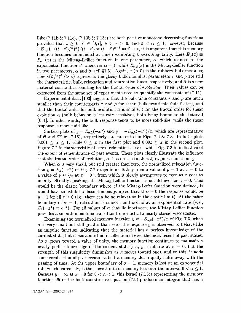
Like (7.11b&:7.11c),(7.13b&=7.13c)areboth positivemonotone-decreasingfunctionsprovided that t > 0, t' E [0, t], p > ¢ > 0, and 0 < _ < 1; however, because

-E_,o(-((t-t')/¢)a)/(t-t ') _ (t-t') _-1 as t' --+ t, it is apparent that this memory

function becomes unbounded at time t exhibiting a weak singularity. Here E_(x) --

E,,l(X) is the Mittag-Leffier function in one parameter, c_, which reduces to the

exponential function e_ whenever a = 1, while E_,z(x) is the Mittag-Leffler function

in two parameters, a and _, (cf. §1.5). Again, _ (> 0) is the rubbery bulk modulus;

now _(fi/¢)a (> _) represents the glassy bulk modulus; parameters "Y and fi are still

the characteristic, bulk, relaxation and retardation times, respectively; and _ is a new

material constant accounting for the fractal order of evolution. Their values can be

extracted from the same set of experiments used to quantify the constants of (7.11).

Experimental data [103] suggests that the bulk time constants _ and fi are much

smaller than their counterparts T and p for shear (bulk transients fade faster), andthat the fractal order for bulk evolution (_ is smaller than the fractal order for shear

evolution a (bulk behavior is less rate sensitive), both being bound to the interval

(0, 1]. In other words, the bulk response tends to be more solid-like, while the shear

response is more fluid-like.

Surface plots of y = Ea,l(-x a) and y = -E_,o(-X_)/x, which are representative

of _ and _ in (7.13), respectively, are presented in Figs. 7.2 & 7.3. In both plots

0.001 < a < 1, while 0 < x in the first plot and 0.001 < x in the second plot.

Figure 7.2 is characteristic of stress-relaxation curves, while Fig. 7.3 is indicative of

the extent of remembrance of past events. These plots clearly illustrate the influence

that the fractal order of evolution, cr, has on the (material) response function, y.

When a is very small, but still greater than zero, the normalized relaxation func-

tion y = E,(-x _) of Fig. 7.2 drops immediately from a value of y = 1 at x = 0 to

a value of y _ 1/2 at x = 0 +, from which it slowly asymptotes to zero as x goes to

infinity. Strictly speaking, the Mittag-Leffier function is not defined for a = 0. This

would be the elastic boundary where, if the Mittag-Leffer function were defined, it

would have to exhibit a discontinuous jump so that at a = 0 the response would be

y = 1 for all x > 0 (i.e., there can be no relaxation in the elastic limit). At the other

boundary of a = 1, relaxation is smooth and occurs at an exponential rate (viz.,

El(-x 1) = e-_). For all values of a that lie inbetween, the Mittag-Leffler function

provides a smooth monotone transition from elastic to nearly classic viscoelastic.

Examining the normalized memory function y -- -E_,o(-X")/x of Fig. 7.3, when

a is very small but still greater than zero, the response y is observed to behave like

an impulse function indicating that the material has a perfect knownledge of the

current state, but it has almost no recollection of even the most recent of past states.

As a grows toward a value of unity, the memory function continues to maintain a

nearly perfect knowledge of the current state (i.e., y is infinite at x = 0, but the

strength of this singularity diminishes as a moves toward one), and to this, it adds

some recollection of past events--albeit a memory that rapidly fades away with the

passing of time. At the upper boundary of a = 1, memory is lost at an exponential

rate which, cureously, is the slowest rate of memory loss over the interval 0 < a < 1.

Because y = oo at x = 0 for 0 < a < 1, this kernel (7.13c) representing the memory

function _ of the bulk constitutive equation (7.9) produces an integral that has a

NASA/T_2002-211914 101

Ea, iH-xa L

a 0o

] 0"8 0 . O"

i

0.8

0.6

x 3

Figure 7.2: A 3D surface plot of y : E_,l(-x_), which appears in the relaxation

function _ of the standard FOV solid.

a 0

0 0.

0. 0. "

1.5

-x-i Ea' 0H-xaL 0

0o

x 3

Figure 7.3: A 3D surface plot of y = -E_,o(-Xa)/x, which appears in the memoryfunction if2 of the standard FOV solid.

NASA/T_2002-211914 102

weak singularity at the upper limit of integration, like the fractional derivative (cf.

Eqn. 1.8a).

Choosing the integral equation of (7.9) (with the bulk relaxation and memory func-

tions being given by Eqns. 7.13b & 7.13c) over its equivalent, fractional, differential

equation (7.13a) has an advantage of disguising the fractal nature of the constitutive

equation. However, selecting _ (7.13b) and 9)I (7.13c) without a priori knowledge

of the fractional differential equation (7.13a) would be unlikely, at least they have

not appeared in the literature as such.$ For this reason, our preferred method for

constitutive construction is to begin with a fractional differential equation, ensuring

that it possesses physically meaningful initial conditions, and to then convert it into

an equivalent integral expression (i.e., to solve the differential equation).

Furthermore, using the integral formulation of (7.9a) with memory function 9)I as

the kernel of integraion, instead of employing its variant (7.9c) that uses the relaxation

function _5 as its kernel, leads to a convolution integral whose recollection of past

events fades much more rapidly, and as such, should be better suited for numerical

analysis.

Alternate model: The viscoelastic models presented in (7.9-7.13) are all based

on Hencky's definition for dilatation, A = lndetF, defined in (4.38). In contrast,

our viscoelastic theory (5.20) introduces a dilational strain measure defined by e --

½(det _F-det F_F_-I),as established in (5.15b), which is a second-order accurate approx-imate t-o Henc-ky dilatation. In fact, whenever the bulk modulus is much stiffer than

the shear modulus for a given material, the trace of (5.20a) produces a hydrostatic

pressure response of

( f0 t ) _ (7.14a)_-p=-_ ¢3a(t)e(O,t)+ ffJta(t-t')e(t',t)dt' when _,a= 2--_Q0'

wherein

1 ( det F det Ft,)c(t',t): '

with F = F(0, t) and F,, = F(0, t'). Assigning to this constitutive equation the

following material functions

I _3_

3(t- t') = 1 + fi3 (-((t - t ), (7.14b)

and

DIa(t- t') = -_at -- t I

(7.14c)

tThis is the first appearance of a memory function that is representative of a fractional-orderviscoelastic model. Relaxation functions representative of fractional-order viscoelastic models havebeen in the literature since Caputo's [12] and Mainardi's [13] pioneering papers, but they have notappeared (e.g., phenomenologically) in the general viscoelastic literature, excluding that subset ofpapers which makes use of the fractional calculus.

NASA/T_2002-211914 103

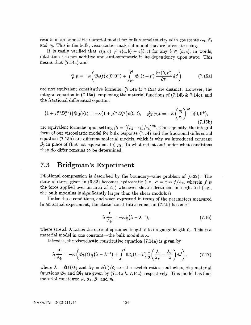
resultsin anadmissiblematerial modelfor bulk viscoelasticitywith constantsa3, 83and w3. This is the bulk, viscoelastic, material model that we advocate using.

It is easily verified that e(a,c) _ e(a,b) + e(b,e) for any b c (a,c); in words,

dilatation e is not additive and anti-symmetric in its dependency upon state. This

means that (7.14a) and

( /0' 1ooop=-t_ _i3(t) e(0, 0 +) + _fi3(t - t') dt' (7.15a)+ Ot'

are not equivalent constitutive formulm; (7.14a & 7.15a) are distinct. However, the

integral equation in (7.15a), employing the material functions of (7.14b & 7.14c), and

the fractional differential equation

o.o.(l+r_3D_,a)(e_p)(t)=-_(l+Pa D, )e(0, t), oo e(0,0+),_- P0+ = --g

(7.15b)are equivalent formuhe upon setting 83 = ((P3 - 7-3)/_-s)aS. Consequently, the integral

form of our viscoelastic model for bulk response (7.14) and the fractional differential

equation (7.15b) are different material models, which is why we introduced constant

83 in place of (but not equivalent to) P3. To what extent and under what conditions

they do differ remains to be determined.

7.3 Bridgman's Experiment

Dilational compression is described by the boundary-value problem of (6.32). The

state of stress given in (6.32) becomes hydrostatic (i.e., (r = ¢ = f/Ao, wherein f is

the force applied over an area of A0) whenever shear effects can be neglected (e.g.,

the bulk modulus is significantly larger than the shear modulus).

Under these conditions, and when expressed in terms of the parameters measured

in an actual experiment, the elastic constitutive equation (7.5b) becomes

f aI(A- A-l), (7.16)A A0 -

where stretch A ratios the current specimen length _ to its gauge length g0- This is amaterial model in one constant--the bulk modulus a.

Likewise, the viscoelastic constitutive equation (7.14a) is given by

( fot l(AAt')dt') (7.17)A Ao _ _3(t) _

where A = g(t)/eo and At, = g(t')/eo are the stretch ratios, and where the material

functions _z and 93t3 are given by (7.14b & 7.14c), respectively. This model has four

material constants: n, a3, 83 and Tz.

NASA/T_2002-211914 104

Appendix A

Table of Caputo Derivatives

For the convenience of the reader, we provide this appendix where we give some

Caputo-type derivatives of certain important functions.* We do not strive for com-

pleteness in any sense, but we do want to give at least the derivatives of the classical

examples.

Throughout this appendix, a will always denote the order of the Caputo-type

differential operator under consideration. We shall only consider the case a > 0 and

_ N, where N := {1,2,3,...} while No := {0,1,2,...}. We use the ceiling function

[c_] to denote the smallest integer greater than (or equal to) a, and the floor function

[cq (= [c_] - 1) to denote the largest integer (strictly) less than c_. Recall that for

a E N, the Caputo differential operator coincides with the usual differential operator

of integer order.

Moreover, E_,, denotes the Mittag-Leffler function of the two parameters # and

> 0, given by (cf. [31, Chp. 18l)

oo tk

= Z r( k +,)'k=0

¢ is the Digamma function, given by

r'(x)¢(x) =

1F1 and 2F1 denote the usual hypergeometric functions, i.e.,

r(b) fi r(a+k) k1Fl(a;b;z) - r(a) _:0 r-_--_k_!z ' a • R, -b _t No,

(sometimes called the Kummer confluent hypergeometric function [1, Chp. 13]), the

power series being convergent for arbitrary complex z, and

F(c)fir(a+k)r(b+k)zk, a, be_t, -c_tNo,

2Fl(a'b;c;z)- F(a)F(b) k=o r(c+ k)k!

*Tables of Riemann-Liouville integrals and derivatives can be found in various places in the

literature (cf. e.g., Podlubny [86] or Samko et al. [102]). We do not repeat those results here.

NASA/T_2002-211914 105

(the Gauss hypergeometric function [1, Chp. 15]), in which case the power series

converges for all complex z with [z[ < 1 and may be extended analytically into the

entire complex plane with a branch cut along the positive real axis from +1 to +oo.

(Note that in the formula below, we only need to evaluate this function for negative

values of z, so the branch cut for positive z gives no problems.) Finally, i = v/_ is

the imaginary unit.

1. Let f(x) = xJ. Here we have to distinguish some cases:

0 if j E No and j < Fa],

r(j+ 1) .(D_f)(z)= r(j+l__)x'-_ifj_Noandj>[a]

orj_Nandj> LaJ.

2. Let f(x) = (x + c)_ for arbitrary c > 0 and j E ]R. Then

(D_f)(x) = r(j + 1) cj-[_]-Ir(j - [aJ)I'([a] -a + 1)zF_l-%Fl(l' [a] -j; [a] -a+ 1;-x/c).

3. Let f(x) = x j lnx for some j > LaJ. Then

L_J

(Da, f)(x) = E(-l)[a]-k+l(_)_ l-_(J- L°_J) "k=o [ k r(j - a + 1) x'-_

r(j + 1) xk-_(¢(j - LaJ) - ¢(j - a + 1) + lnz).+ F(j--- a + 1)

4. Let f(x) = exp(jx) for some j E N. Then

D _ =(,f)(x) j['_lxF'_l-'_El,[,_l_,_+x(jx).

5. Let f(x) = sinjx for some j E JR. Here again we have two cases:

JF li(-1)r°V2xr l- [1F1(1; - a + 1;ijx)2r(fal - a + 1)

- 1Fl(1; Fal - a + 1;-ijx)] if Fal is even,

(D_f)(x)= jral(-1)L_Jl2xFc_l-a [1Fl(1; [a]-a+ 1;ijx)2r(r l - + 1)

+ 1FI(1; pal - a + 1;-ijx)] if [a 1 is odd.

6. Finally we consider f(x) = cosjx with some j E R. As in the previous example,we obtain two cases:

jr:l(_l) rOv2xr:l-:2r([c_l -a+ 1) [_Ft(1; [c_l-a+ 1;ijx)

+ 1FI(1; [a] -a + 1;-ijx)] if [a] is even,

(Dyf)(x) = jF_li(_l)tOj/2xF_l__

2r(F_l-_+ 1) [1Fl(1; Fal-a+ 1;ijx)

- 1FI(1; [(_l - a + 1;-ijx)] if [a] is odd.

NASA/T_2002-211914 106

Appendix B

Automatic Integration

In §1.5.2 we had found the need to calculate two integrals numerically in order to

complete the evaluation of the Mittag-Leffler function. In this appendix we outline a

possible strategy for the solution of these integrals. Essentially we will follow the ideas

explained in QUADPACK [84]. The routines introduced in that book are the generally

accepted standard when looking for efficient and reliable quadrature algorithms. They

are in the public domain, but they can also be found in many commercially distributed

software packages. The source code is written in FORTRAN77 and may be obtained,

for example, from the URL http://www.netlib.org/quadpack. For integrands of

the form encountered in §1.5.2, it turns out that the routine DQAG (Double precision

Quadrature, Adaptive, General purpose) is the method of choice. Our description of

this routine follows a top-down structure (i.e., we first explain the general strategy

without giving much information on the details, and at a later stage we fill in those

details).

B.1 The Fundamental Strategy

The fundamental idea of automatic integration is the following. The user supplies the

integrand function and the bounds for the interval of integration (i.e., the data that

define the integral in question) and a desired accuracy (i.e., a bound for the relative

or absolute error that he/she is willing to accept). The routine is then supposed to

return either an approximation for the correct value of the integral that is sufficiently

accurate to satify the user's requirements or an error flag if it fails to find such an

approximation.

Typically the algorithms try to achieve this goal by sub-dividing the interval of

integration in an adaptive way, thus concentrating more quadrature nodes in areas

where the integrand is difficult to approximate. This leads to a structure indicated

in Alg. B.1.

In practice, one may also terminate the WHILE loop in this algorithm when;

for example, too many sub-divisions have taken place thereby using up all available

memory, or too much computing time has been consumed. In such cases the algorithm

should return an error flag.

NASA/T_2002-211914 107

Algorithm B.1 Automatic IntegrationGIVEN two realnumbersa and b, a function f : [a, b] -+ C,

and some tolerance e > 0 THEN

Calculate an approximation Q[f] for f: f(x)dx and an estimate _ for the

error S(x)dx- Q[S]Initialize a list L of the approximations obtained so far

by L := { ([a, b], Q[f], _)}WHILE error tolerance is not satified DO

Take the interval from L with the largest error estimate

and remove it from the list;

Bisect this interval;

Calculate approximations and error estimates for the two newly obtained

subintervals;

Add these subintervals, their corresponding approximations,

and their error estimates to the list L

END of while loop

RETURN the sum of the approximations obtained for all the intervals.

B.2 Approximation of the Integral

In Alg. B.1 we have left open some of the key details. Specifically, we have not

said how the approximation of the integral itself will be performed, and we have not

indicated how the required error estimates can be found. We now turn our attention

to these two questions.

The basic idea behind the solution is the concept of Gauss-Kronrod integration.

That is, we calculate two different approximations for the integral, both of which are

of the formn

Za.S(x.,),5=1

with suitably chosen values of n, aj,n, and xj,_ (j = 1,...,n). In particular, we

begin with a first approximation that is just a Gauss quadrature formula with nl

nodes, which is the (uniquely determined) quadrature formula that gives the exact

value of the integral whenever the integrand is a polynomial of degree not exceeding

2nl - 1. This formula has been thoroughly investigated. For a recent survey we

refer to Ref. [10] and the references cited therein. Specifically, there is no quadrature

formula with the same number of nodes that is exact for a larger class of polynomials.

Moreover, as stated in [10], both theoretical and practical evidence suggest that this

method is a very good one.

B.3 Approximation of Error Estimates

From rather general considerations, it is known that one, single, quadrature formula

can only give an approximation, but not both an approximation and an error estimate.

NASA/T_2002-211914 108

Therefore, to derive also an error estimate, it is necessary to introduce a second

quadrature formula. The heuristic argument is as follows. Assuming that the second

quadrature formula is much more accurate than the first, then the difference between

the two approximations will be a good approximation for the error of the cruder of

the two approximations, and therefore, a rather conservative (and thus quite reliable)

upper bound for the error of the finer of the two approximations. Hence, we need

a second quadrature formula that is significantly better than the first (Gauss-type)

formula. In view of the quality of the Gauss formula, this can only be achieved by

selecting a formula with n2 nodes, where n2 > nl. In principle, one could use a Gauss

formula again, but this would be very uneconomical because a Gauss formula with

nl nodes would have at most one node in common with a Gauss formula with n2

nodes, and so almost none of the information gathered so far (i.e., the function values

f (xj,,_ 1), whose calculation is typically the most computationally expensive part of the

algorithm) could be reused. To overcome this difficulty, Kronrod [59, 60] suggested

to construct a formula that is nowadays called the Kronrod extension of the Gauss

formula or, shortly, the Gauss-Kronrod formula. His formula is based on the Gauss

formula with nl nodes; it uses n2 = 2nl + 1 nodes and is constructed according to

the following criteria:

• The nl nodes xj, m of the Gauss method form a subset of the n2 nodes xj,._, ofthe Gauss-Kronrod method.

• The remaining nodes and the weights aj,n2 of the of the Gauss-Kronrod scheme

are determined in such a way that the resulting method is exact for all polyno-

mials of degree not exceeding 3nl + 1.

A recent survey on Gauss-Kronrod formulas is given in [29].

Algorithms for the concrete calculation of the required nodes and weights are

available (cf. the survey papers mentioned above and the references cited therein).

For our purposes, it is sufficient to use the tabulated values given in [84]. In particular,

following the suggestions made there, we propose using the Gaussian method with

15 points in combination with the 31-point Kronrod extension for computing the

integral with function K mentioned in Alg. 1.4 (the monotonic part). In view of the

nice smoothness properties of the integrand, this gives us an approximation with quite

high accuracy without too much computational effort. For the other integral in that

algorithm, with the oscillatory integrand function P, these formulm may be unable

to follow the oscillations properly; thus, we propose using the 30-point Gauss method

together with its 61-point Kronrod extension. This is essentially also the method

suggested for oscillatory integrals in the NAG Library [81] (see the documentation

for routine D01AKF).

NASA/T_2002-211914 109

Appendix C

Table of Pad Approximates for

Mittag-Leffier Function

This appendix presents a scheme for fast computations of

E_(-x_), 0<c_<l, x>_0,

suitable for finite elements. This function appears in the relaxation functions of both

the FOV fluid (2.1) and solid (2.2).

The defining series (1.11) is used on the interval 0 < x < 0.1, and an asymptotic

series (1.16) is used whenever x > 15, as in Alg. 1.4, but in contrast with Alg. 1.4, a

Pad_ approximate (or rational polynomial) is applied inbetween where 0.1 _< x _< 15;

specifically,

'_4 (-x) ak

z--,k=0 r(-Y4-_) 0 _< x _< 0.1

Ea(-x _) _ a0+alx+a2x2 0.i < x < 15 (C.1)l +bl x +b2x2-I-b3 m-O a

X--_4 (-x) -ak- z_,k=l _ x _> 15

where the coefficients a0, al, a2, bl, b2 and b3 are listed in Table C.1 for values of a

varying between 0.01 and 0.99 by increments of 0.01. Also listed are the r 2 resultants

from each nonlinear regression with the tolerance set sufficient to achieve accuracies

of r 2 > 0.999, except for a > 0.9 where such tight r 2 values could not be achieved for

the order of approximate employed. The Pad6 approximates were obtained from fits

to exact values (within machine precision) for the Mittag-Leffier function (obtained

from Alg. 1.4) at 150 evenly spaced grid points over the interval [0.1, 15]. The form

of this rational polynomial was selected after a study of numerous tables for function

approximation listed in the appendices of Hart et al. [48]. Our fits were constrained

to be exact at the end points so that transitions will be smooth when crossing a

boundary between solution domains.

A number written as 0.123456(7) stands for 0.123456. l0 T = 1,234,560.

NASA/TM--2002-211914 111

Table C.I: Coefficients for Pad_ approximates of Mittag-Lefller function.

ao

0.01 -.424129(3)

0.02 -.291078(4)

0.03 -.159594(4)

0.04 -.401668(4)0.05 -.480619(4)

0.06 -.358700(4)0.07 -.431271(4)

0.08 -.104813(5)

0.09 -.113182(5)

0.10 -.100534(5)

0.11 -.771890(4)

0.12 -.209949(4)

0.13 -.201966(5)

0.14 -.144185(5)

0.15 -.358699(4)

0.16 -.367384(5)

0.17 -.834348(4)

0.18 -.665920(4)

0.19 -.880313(4)

0.20 -.516937(4)0.21 -.181654(5)

0.22 -.287739(5)

0.23 -.283969(5)

0.24 -.218950(5)

0.25 -.184865(5)

0.26 -.154930(5)

0.27 -.252656(5)

0.28 -.348286(5)

0.29 -.223178(5)

0.30 -.262152(5)

0.31 -.110316(5)

0.32 -.344887(5)

0.33 -.253440(5)0.34 -.320037(5)

0.35 -.788648(5)

0.36 -.289781(5)

0.37 -.142051(5)

0.38 -.816551(5)0.39 -.575871(5)

0.40 -.173808(5)

0.41 -.103477(5)

0.42 -.195086(5)

0.43 -.333165(5)

0.44 -.473286(5)0.45 -.147598(5)

0.46 -.152914(5)0.47 -.167037(5)

0.48 -.142611(5)

0.49 -.654706(5)

0.50 -.188800(3)

0.51 -.516448(5)

0.52 -.392154(5)

0.53 -.135449(5)

0.54 -.953841(4)

0.55 -.793386(3)

0.56 -.599232(4)

al a2 bl b2 b3

-.695856(6) -.391944(6) -.138637(7) -.795778(6) -.207400(3)

-.231705(7) -.121393(7) -.460100(7) -.250385(7) -.127923(4)

-.883786(6) -.485177(6) -.174711(7) -.101562(7) -.832687(3)

-.151329(7) -.678102(6) -.298958(7) -.144743(7) -.138260(4)

-.145550(7) -.643881(6) -.286638(7) -.139751(7) -.171118(4)

-.953746(6) -.452754(6) -.186815(7) -.996694(6) -.160873(4)

-.958824(6) -.424475(6) -.187447(7) -.952144(6) -.175012(4)

-.220562(7) -.109649(7) -.427837(7) -.248747(7) -.594850(4)

-.204162(7) -.931135(6) -.395568(7) -.215524(7) -.560193(4)

-.165546(7) -.753470(6) -.319371(7) -.177305(7) -.527749(4)

-.116952(7) -.530686(6) -.224658(7) -.126954(7) -.429168(4)

-.331485(6) -.178194(6) -.628014(6) -.428531(6) -.183967(4)

-.264628(7) -.118361(7) -.503944(7) -.292906(7) -.123451(5)

-.177380(7) -.787251(6) -.336281(7) -.198184(7) -.923408(4)

-.414163(6) -.180624(6) -.782040(6) -.463020(6) -.235432(4)

-.387982(7) -.157708(7) -.732069(7) -.414017(7) -.218683(5)

-.877610(6) -.381391(6) -.163991(7) -.101120(7) -.619007(4)

-.661019(6) -.279508(6) -.123090(7) -.755801(6) -.495376(4)

-.839225(6) -.352670(6) -.155465(7) -.970538(6) -.689880(4)

-.463982(6) -.186660(6) -.857478(6) -.525412(6) -.391939(4)

-.159929(7) -.655973(6) -.293380(7) -.187316(7) -.153968(5)

-.241617(7) -.962412(6) -.441685(7) -.280701(7) -.244057(5)

-.233523(7) -.935683(6) -.423970(7) -.277398(7) -.261404(5)

-.174274(7) -.687682(6) -.314803(7) -.207911(7) -.208550(5)

-.142847(7) -.555414(6) -.256670(7) -.171282(7) -.182554(5)

-.116572(7) -.448241(6) -.208289(7) -.140906(7) -.159998(5)

-.187367(7) -.720787(6) -.332362(7) -.230555(7) -.280571(5)

-.250157(7) -.938597(6) -.441764(7) -.306951(7) -.392527(5)

-.158819(7) -.597404(6) -.278265(7) -.198723(7) -.272201(5)

-.180630(7) -.659350(6) -.315184(7) -.224602(7) -.321389(5)

-.741001(6) -.263517(6) -.128658(7) -.919175(6) -.137449(5)

-.231540(7) -.831618(6) -.398374(7) -.294522(7) -.473795(5)

-.165943(7) -.579558(6) -.284133(7) -.210336(7) -.352888(5)

-.206983(7) -.712936(6) -.351975(7) -.264342(7) -.467058(5)

-.506620(7) -.172863(7) -.854865(7) -.654223(7) -.122026(6)

-.195379(7) -.707274(6) -.324061(7) -.268137(7) -.555978(5)

-.971770(6) -.354821(6) -.159385(7) -.136569(7) -.302386(5)

-.523578(7) -.175872(7) -.860767(7) -.705295(7) -.156056(6)

-.348533(7) -.107617(7) -.574012(7) -.450994(7) -.991720(5)

-.117277(7) -.408516(6) -.187857(7) -.167833(7) -.429558(5)

-.686777(6) -.231234(6) -.109392(7) -.977034(6) -.258727(5)

-.129617(7) -.429282(6) -.204698(7) -.185582(7) -.514821(5)

-.221252(7) -.718492(6) -.346552(7) -.318194(7) -.922518(5)

-.311742(7) -.981295(6) -.484992(7) -.447200(7) -.134275(6)

-.982326(6) -.304968(6) -.151324(7) -.142189(7) -.447789(5)

-.104712(7) -.326140(6) -.159246(7) -.154553(7) -.517302(5)

-.114533(7) -.346912(6) -.172774(7) -.169118(7) -.587605(5)

-.991368(6) -.293586(6) -.148061(7) -.147062(7) -.531760(5)

-.455618(7) -.130849(7) -.675094(7) -.675481(7) -.253173(6)

-.135370(5) -.383675(4) -.198223(5) -.202768(5) -.797517(3)

-.373170(7) -.102716(7) -.541357(7) -.559798(7) -.228252(6)

-.289687(7) -.780114(6) -.415703(7) -.437101(7) -.185908(6)

-.106392(7) -.289899(6) -.150142(7) -.164334(7) -.749106(5)

-.748349(6) -.193214(6) -.104887(7) -.114460(7) -.530462(5)

-.639333(5) -.159875(5) -.886439(5) -.979799(5) -.469973(4)

-.443865(6) -.952614(5) -.619108(6) -.646389(6) -.288690(5)

T 2

0.9993710.999345

0.999381

0.999114

0.9991290.999313

0.999215

0.999401

0.999340

0.999361

0.999382

0.999349

0.999408

0.999420

0.999423

0.999358

0.999453

0.999452

0.999463

0.999446

0.999480

0.999477

0.999497

0.999503

0.999510

0.999520

0.999534

0.999538

0.999553

0.999556

0.999558

0.999578

0.999583

0.999592

0.999604

0.999616

0.999617

0.999642

0.999625

0.999651

0.999700

0.999681

0.999693

0.999708

0.999719

0.999725

0.999740

0.999752

0.999766

0.999777

0.999790

0.999801

0.999802

0.999822

0.999835

0.999847

NASA/T_2002-211914 112

TableC.1:CoefficientsforPad6approximatesofMittag-Leffierfunction.

ao

0.57 -.337393(5)

0.58 -.463960(5)0.59 -.151791(4)0.60 -.502729(4)

0.61 -.480103(5)

0.62 -.671512(4)0.63 -.312780(5)

0.64 -.567954(5)

0.65 -.149230(4)

0.66 -.433396(5)

0.67 -.752321(4)

0.68 -.503149(5)

0.69 -.113475(5)

0.70 -.277604(3)

0.71 -.551694(5)

0.72 -.310305(5)

0.73 -.160766(4)0.74 0.341935(4)

0.75 0.173763(4)

0.76 -.198004(4)0.77 -.255574(4)

0.78 -.107310(4)

0.79 -.494450(4)

0.80 -.218066(4)

0.81 -.534378(4)

0.82 -.675467(4)

0.83 -.702848(3)0.84 -.609980(4)

0.85 -.103053(5)

0.86 -.774771(4)

0.87 -.838904(4)

0.88 -.447750(4)

0.89 -.390787(4)

0.90 -.724688(4)

0.91 -.152262(5)

0.92 -.150108(5)

0.93 -.106495(5)0.94 -.153906(5)

0.95 -.600332(4)

0.96 -.445797(5)

0.97 -.355171(5)0.98 -.145397(5)

0.99 -.105996(5)

al as bl b2 b3

-.286190(7) -.663678(6) -.388535(7) -.438767(7) -.223581(6)

-.405168(7) -.899289(6) -.544254(7) -.620515(7) -.324201(6)

-.125852(6) -.241507(5) -.169238(6) -.185486(6) -.904156(4)

-.464569(6) -.919187(5) -.611566(6) -.705142(6) -.377940(5)

-.461103(7) -.860143(6) -.600297(7) -.697998(7) -.378472(6)

-.708363(6) -.131044(6) -.906252(6) -.108843(7) -.626832(5)

-.328986(7) -.533551(6) -.418611(7) -.494518(7) -.268704(6)

-.632239(7) -.945394(6) -.794766(7) -.947107(7) -.509518(6)

-.182752(6) -.259499(5) -.226154(6) -.275373(6) -.151317(5)

-.549988(7) -.664464(6) -.674519(7) -.815645(7) -.407908(6)

-.109682(7) -.126030(6) -.132094(7) -.164296(7) -.843703(5)

-.782828(7) -.716973(6) -.932883(7) -.115421(8) -.500161(6)

-.204800(7) -.158167(6) -.240096(7) -.301897(7) -.117538(6)

-.535397(5) -.226639(4) -.621910(5) -.768192(5) -.150446(4)

-.158192(8) -.673086(6) -.178833(8) -.232888(8) -.532630(6)

-.102892(8) 0.663348(5) -.115056(8) -.146317(8) 0.202771(6)-.449254(7) -.116371(6) -.482429(7) -.682061(7) -.111373(6)

-.241906(7) -.669717(5) -.252295(7) -.376790(7) -.808538(5)

-.103357(7) -.513330(6) -.106853(7) -.212490(7) -.787594(6)

-.170209(6) -.546410(6) -.212224(6) -.727938(6) -.906762(6)

-.399973(6) -.408010(6) -.461840(6) -.889107(6) -.736776(6)

-.102865(6) -.104591(6) -.125079(6) -.207143(6) -.205284(6)

-.463767(6) -.357502(6) -.563528(6) -.802633(6) -.767703(6)

-.219047(6) -.128115(6) -.262855(6) -.339154(6) -.302753(6)

-.539996(6) -.258539(6) -.645497(6) -.766988(6) -.675138(6)

-.688012(6) -.275764(6) -.819312(6) -.908437(6) -.800006(6)

-.690578(5) -.240789(5) -.824283(5) -.847142(5) -.779293(5)

-.583751(6) -.176849(6) -.697471(6) -.667838(6) -.642815(6)

-.915547(6) -.247199(6) -.110278(7) -.963517(6) -.101397(7)

-.667011(6) -.156824(6) -.805409(6) -.651177(6) -.733497(6)

-.693431(6) -.141730(6) -.840712(6) -.624128(6) -.763282(6)

-.359964(6) -.629983(5) -.437447(6) -.299094(6) -.396021(6)

-.296304(6) -.446099(5) -.362820(6) -.222076(6) -.331368(6)

-.509096(6) -.654940(5) -.630388(6) -.335377(6) -.584487(6)

-.100158(7) -.106340(6) -.125254(7) -.574996(6) -.117309(7)

-.942028(6) -.792810(5) -.118669(7) -.467003(6) -.112366(7)

-.626399(6) -.398859(5) -.797901(6) -.255226(6) -766267(6)

-.847297(6) -371308(5) -.109242(7) -.268144(6) -.106481(7)

-.311566(6) 0.756057(4) -.406277(6) -.710353(5) -.401715(6)

-.214492(7) -.119855(5) -.284119(7) -.270455(6) -.285641(7)

-.159674(7) 0.206708(5) -.214673(7) -.423690(5) -.219239(7)

-.610793(6) 0.190402(5) -.834188(6) 0.464083(5) -.865369(6)

-.416113(6) 0.204340(5) -.577797(6) 0.755603(5) -.608788(6)

r _

0.999859

0.9998710.999886

0.9998960.999907

0.999908

0.999928

0.999937

0.999939

0.999953

0.999948

0.999960

0.999955

0.999976

0.999919

0.99994

0.999719

0.999510

0.999166

0.999483

0.999574

0.999673

0.999707

0.999721

0.999723

0.999715

0.999699

0.999674

0.999639

0.999594

0.999538

0.999468

0.999382

0.999277

0.999150

0.998998

0.998816

0.998600

0.998343

0.998041

0.997685

0.997270

0.996786

NASA/T_2002-211914 113

Bibliography

[1] M. Abramowitz and I. A. Stegun (eds.), Handbook of mathematical functions: With formulas,graphs, and mathematical tables, NBS Applied Mathematics Series, vol. 55, National Bureau of

Standards, Washington, D.C., 1964, Second printing with corrections. Republished by Dover,New York, 1965.

[2] E. Almansi, Sulle deformazioni finite dei solidi elastici isotropi, Rendiconti della Reale Ac-cademia dei Lincei: Classe di scienze fisiche, matematiche e naturali 20 (1911), 705-714.

[3] R.L. Bagley and R. A. Calico, Fractional order state equations for the control of viscoelasticallydamped structures, Journal of Guidance, Control, and Dynamics 14 (1991), 304-311.

[4] R. L. Bagley and P. J. Torvik, A theoretical basis for the application of fractional calculus toviscoelasticity, Journal of Rheology 27 (1983), 201-210.

[5] __, On the fractional calculus model of viscoelastic behavior, Journal of Rheology 30(1986), 133-155.

[6] Z. P. Ba_ant, Easy-to-compute tensors with symmetric inverse approximating Hencky finitestrain and its rate, Journal of Engineering Materials and Technology 120 (1998), 131-136.

[7] B. Bernstein, E. A. Kearsley, and L. J. Zapas, A study of stress relaxation with finite strain,Transactions of the Society of Rheology 7 (1963), 391-410.

[8] G.W. Scott Blair, Analytical and integrative aspects of the stress-strain-time problem, Journalof Scientific Instruments 21 (1944), 80-84.

[9] L. Boltzmann, Zur Theorie der elastischen Nachwirkung, Sitzungsberichte der KaiserlichenAkademie der Wissenschaften: Mathematisch-naturwissenschaftlichen klasse, Wien 70 (1874),

275-300.

[10] H. Brass, J.-W. Fischer, and K. Petras, The Gaussian quadrature method, Abhandlungen derBraunschweigischen Wissenschaftlichen Gesellschaft 47 (1996), 115-150.

[11] P.W. Bridgman, The compressibility of thirty metals as a function of pressure and temperature,Proceedings of the American Academy of Arts and Sciences 58 (1923), 165-242.

[12] M. Caputo, Linear models of dissipation whose Q is almost frequency independent-II, TheGeophysical Journal of the Royal Astronomical Society 13 (1967), 529-539.

[13] M. Caputo and F. Mainardi, Linear models of dissipation in anelastic solids, Rivista del Nuovo

Cimento 1 (1971), 161-198.

[14] A.-L. Cauchy, Exercices de mathdmatiques, vol. 2, de Bure Fr_res, Paris, 1827.

NASA/T_2002-211914 115

[15] J.-T. Chern, Finite element modeling of viscoelastic materials on the theory of fractional cal-culus, Ph.D. thesis, The Pennsylvania State University, December 1993, University MicrofilmsNo. 9414260.

[16] R. M. Christensen, Theory of viscoelasticity: An introduction, Academic Press, New York,1971.

[17]

[18]

[19]

[20]

[21]

[22]

[23]

K. S. Cole and R. H. Cole, Dispersion and absorption in dielectrics: L alternating current

characteristics, Journal of Chemical Physics 9 (1941), 341-351.

B. D. Coleman, Thermodynamics of materials with memory, Archive for Rational Mechanics

and Analysis 17 (1964), 1-46.

B. D. Coleman and V. J. Mizel, On the general theory of fading memory, Archive for RationalMechanics and Analysis 29 (1968), 18-31.

K. Diethelm, Generalized compound quadrature formulce for finite-part integrals, IMA Journalof Numerical Analysis 17 (1997), 479-493.

K. Diethelm and N. J. Ford, Analysis of fractional differential equations, Journal of Mathe-matical Analysis and Applications 265 (2002), in press.

K. Diethelm, N. J. Ford, and A. D. Freed, Detailed error analysis for a fractional Adamsmethod, In review.

[24]

[25]

[26]

[271

[2sl

[29]

__, A predictor-corrector approach for the numerical solution of fractional differential

equations, Nonlinear Dynamics ?? (2002), in press.

K. Diethelm and G. Walz, Numerical solution of fractional order differential equations byextrapolation, Numerical Algorithms 16 (1997), 231-253.

J. F. Douglas, Polymer science applications of path-integration, integral equations, and frac-

tional calculus, Applications of Fractional Calculus in Physics (R. Hilfer, ed.), World Scientific,Singapore, 2000, pp. 241-330.

T. C. Doyle and J. E. Ericksen, Nonlinear elasticity, Advances in Applied Mechanics (H. L.

Dryden and T. von K_rm_n, eds.), vol. 4, Academic Press, New York, 1956, pp. 53-115.

A. D. Drozdov, Fractional differential models in finite viscoelasticity, Acta Mechanica 124

(1997), 155-180.

D. C. Drucker, A definition of stable inelastic material, Journal of Applied Mechanics 27

(1959), 101-106.

S. Ehrich, Stieltjes polynomials and the error of Gauss-Kronrod quadrature formulas, Appli-

cations and Computation of Orthogonal Polynomials (W. Gantschi, G. Golub, and G. Opfer,eds.), International Series of Numerical Mathematics, no. 131, Birkh_user, Basel, 1999, pp. 57-77.

[30] D. Elliott, An asymptotic analysis of two algorithms for certain Hadamard finite-part integrals,

IMA Journal of Numerical Analysis 13 (1993), 445-462.

[31] A. Erd_lyi, W. Magnus, F. Oberhettinger, and F. G. Tricomi (eds.)i Higher transcendental

functions, Bateman manuscript project, vol. 2, McGraw-Hill, New York, 1955.

[32] J. Finger, Uber die allgemeinsten Beziehungen zwischen endlichen Deformationen und

den zugehSrigen Spannungen in aeolotropen und isotropen Substanzen, Sitzungsberichte derAkademie der Wissenschaften, Wien 103 (1894), 1073-1100.

NASA/T_2002-211914 116

[33]E. R. Fitzgerald,Jr. L. D. Grandine,andJ. D. Ferry,Dynamic mechanical properties ofpolyisobutylene, Journal of Applied Physics 24 (1953), 650-655.

[34] P. J. Flory, Thermodynamic relations for high elastic materials, Transactions of the Faraday

Society 57 (1961), 829-838.

[35] N. J. Ford and A. C. Simpson, The numerical solution of fractional differential equations:Speed versus accuracy, Numerical Algorithms 26 (2001), 333-346.

[36] A. D. Freed, Natural strain, Journal of Engineering Materials and Technology 117 (1995),379-385.

[37] S. Fujiwara and F. Yonezawa, Anomalous relaxation in ffactal structures, Physical Review E

51 (1995), 2277-2285.

[38] A. Gemant, A method of analyzing experimental results obtained from elasto-viscous bodies,

Physics 7 (1936), 311-317.

[39] A. N. Gent and R. S. Rivlin, Experiments on the mechanics of rubber I: Eversion of a tube,

Proceedings of the Physical Society, London B 65 (1952), 118-121.

[40] __, Experiments on the mechanics of rubber II: The torsion, inflation and extension of a

tube, Proceedings of the Physical Society, London B 65 (1952), 487-501.

[41] __, Experiments on the mechanics of rubber III: Small torsions of stretched prisms, Pro-ceedings of the Physical Society, London B 65 (1952), 645-648.

[421 A. N. Gerasimov, A generalization of linear laws of deformation and its application to innerfriction problems, Prikladna_ila Matematika i Mekhanika 12 (1948), 251-260.

[43] S. Gomi and F. Yonezawa, Anomalous relaxation in the fractal time random walk model,Physical Review Letters 74 (1975), 4125-4128.

[44] R. Gorenflo, Fractional calculus: Some numerical methods, Fractals and Fractional Calculusin Continuum Mechanics (A. Carpinteri and F. Mainardi, eds.), CISM Courses and Lectures,

no. 378, Springer, Wien, 1997, pp. 277-290.

[45] R. Gorenflo, I. Loutchko, and Yu. Luchko, Numerische Berechnung der Mittag-Leffler - Funk-

tion Ea,z(z) und ihrer Ableitung, Tech. Report A-6-99, Freie Universit_it Berlin, Berlin, 1999.

[46] G. Green, On the propagation of light in crystallized media, Transactions of the CambridgePhilosophical Society 7 (1841), 121-140.

[47] M. E. Gurtin and E. Sternberg, On the linear theory of viscoelasticity, Archive for Rational

Mechanics and Analysis 11 (1962), 291-356.

[48] J. F. Hart, E. W. Cheney, C. L. Lawson, H. J. Maehly, C. K. Mesztenyi, J. R. Rice, H. G.

Thacher, Jr., and C. Witzgall, Computer approximations, The SIAM Series in Applied Math-

ematics, John Wiley & Sons, New York, 1968.

[49] H. Hencky, Uber die Form des Elastizitiitsgesetzes bei ideal elastischen Stoffen, Zeitschrift ffir

technische Physik 9 (1928), 215-220.

[50] __, The law of elasticity for isotropic and quasi-isotropic substances by finite deforma-

tions, Journal of Rheology 2 (1931), 169-176.

[51] A. Hoger, The material time derivative of logarithmic strain, International Journal of Solidsand Structures 22 (1986), 1019-1032.

NASA/T_2002-211914 i 17

[52]F. deHoogandR. Weiss,Asymptotic expansions for product integration, Mathematics ofComputation 27 (1973), 295-306.

[53] H. M. James and E. Guth, Theory of the elastic properties of rubber, The Journal of ChemicalPhysics 11 (1943), 455-481.

[54] G. Jaumann, Die Grundlagen der Bewegungslehre yon einem modernen Standpunkte aus, Ver-lag, Leipzig, 1905.

[55l __ , Geschlossenes System physikalischer und chemischer Differentialgesetze, Sitzungs-berichte der Kaiserlichen Akademie der Wissenschaften: Mathematisch naturwis-

senschaftliche klasse 120 (1911), 385-530.

[56] A. Kaye, Non-Newtonian flow in incompressible fluids, Tech. Report 134, The College ofAeronautics, Cranfield, October 1962.

[57]

[58]

A. A. Kilbas and J. J. Trujillo, Differential equations of fractional order: Methods, results and

problems-I, Applicable Analysis 78 (2001), 153-192.

G. Kirchhoff, iiber die Gleichungen des Gleichgewichtes eines elastischen KSrpers bei nichtunendlich kleinen Verschiebungen seiner Theile, Sitzungsberichte der Akademie der Wis-senschaften, Wien 9 (1852), 763-773.

[59] A. S. Kronrod, Integration with control o] accuracy, Soviet Physics Doklady 9 (1964), no. 1,17-19.

[60] __, Nodes and weights for quadrature formulce: Sixteen place tables, Nauka, Moscow,1964, In Russian.

[61] Y. Kwon and K. S. Cho, Time-strain nonseparability in viscoelastic constitutive equations,

Journal of Rheology 45 (2001), 1441-1452.

[62] R. S. Lakes, Viscoelastic solids, CRC Press, Boca Raton, 1998.

[63] A. I. Leonov, On a class of constitutive equations for viscoelastic liquids, Journal of Non-Newtonian Fluid Mechanics 25 (1987), 1-59.

[64] __, On the constitutive equations for nonisothermal bulk relaxation, Macromolecules 29(1996), 8383-8386.

[65] __ , Constitutive equations for viscoelastic liquids: Formulation, analysis and compari-son with data, Advances in the Flow and Rheology of Non-Newtonian Fluids (D. A. Siginer,D. DeKee, and R. P. Chalra, eds.), vol. A, Elsevier, New York, 1999, pp. 519-575.

[66] __, On the conditions of potentiality in finite elasticity and hypo-elasticity, International

Journal of Solids and Structures 37 (2000), 2565-2576.

[67] J. Liouville, Mgmoire sur quelques questions de gdomdtrie et de mdcanique, et sur un nou-

veau genre de calcul pour rdsoudre ces questions, Journal de l'I_cole Polytechnique 13 (1832),no. cahier 21, 1-66.

[68] A. S. Lodge, Elastic liquids: An introductory vector treatment of finite-strain polymer theology,Academic Press, London, 1964.

[69] __, On the description of rheological properties of viscoelastic continua. L Body-, space-,

and Cartesian-space - tensor fields, Rheological Acta 11 (1972), 106-118.

NASA/T_2002-211914 118

[70] __

[71]

[72]

[73]

[74]

[75]

[76]

[77[

[78]

[79]

, Body tensor fields in continuum mechanics: With applications to polymer rheology,

Academic Press, New York, 1974.

__, 1980, Course notes, University of Wisconsin, Madison.

__, An introduction to elastomer molecular network theory, Bannatek Press, PO Box

44133, Madison, WI, 1999, Has no ISBN.

C. F. Lorenzo and T. T. Hartley, Initialized fractional calculus, TP 2000-209943, NASA GlennResearch Center, Cleveland, February 2000.

J. Liitzen, 2001, Personal communication.

F. Malnardi, Fractional calculus: Some basic problems in continuum and statistical mechanics,Fractals and Fractional Calculus in Continuum Mechanics (A. Carpinteri and F. Mainardi,

eds.), CISM Courses and Lectures, no. 378, Springer, Wien, 1997, pp. 291-348.

F. Mainardi and R. Gorenflo, The Mittag-Leffler function in the Riemann-Liouville fractional

calculus, Boundary Value Problems, Special Functions and Fractional Calculus. Proceedingsof international conference dedicated to 90th birthday of Prof. F. D. Gakhov (Minsk) (A. A.

Kilbas, ed.), Belarusian State University, February 1996, pp. 215-225.

R. S. Marvin, R. Aldrich, and H. S. Sack, The dynamic bulk viscosity of polyisobutylene,Journal of Applied Physics 25 (1954), 1213-1218.

K. S. Miller and B. Ross, An introduction to the fractional calculus and fractional differentialequations, John Wiley & Sons, New York, 1993.

G. Mittag-Leffier, Sur la reprdsentation analytique d'une branche uniforme d'une fonctionmonog_ne, Acta Mathematica 29 (1904), 101-168.

[80] M. Mooney, A theory of large elastic deformations, Journal of Applied Physics 11 (1940),582-592.

[81]

[821

[83]

[84]

[85]

[86]

[871

Numerical Algorithms Group, Ltd., Oxford, NAG FORTRAN library mark 17, 1995.

K. B. Oldham and J. Spanier, The fractional calculus, Mathematics in Science and Engineering,Academic Press, New York, 1974.

J. G. Oldroyd, On the formulation of theological equations of state, Proceedings of the Royal

Society, London A 200 (1950), 523-541.

R. Piessens, E. de Doncker-Kapenga, C. Uberhuber, and D. K. Kahaner, QUADPACK--A

subroutine package for automatic integration, Springer Series in Computational Mathematics,

Springer, Berlin, 1983.

G. Piola, La meccanica dd corpi naturalmente estesi: Trattata col calcolo delle variazioni,

Opuscoli Matematici e Fisici di Diversi Autori 1 (1833), 201-236.

I. Podlubny, Fractional differential equations: An introduction to fractional derivatives, frac-tional differential equations, to methods of their solution and some of their applications, Math-

ematics in Science and Engineering, vol. 198, Academic Press, San Diego, 1999.

__, Geometric and physical interpretation of fractional integration and fractional differen-

tiation, Tech. report, Department of Informatics and Control Engineering, Technical University

of Kosice, 2001.

NASA/T_2002-211914 119

[88] J. H. Poynting, On pressure perpendicular to the shear planes in finite pure shears, and onthe lengthening of loaded wires when twisted, Proceedings of the Royal Society, London A 82

(1909), 546-559.

[89] W. H. Press, S. A. Teukolsky, W. T. Vetterling, and B. P. Flannery, Numerical recipes inC: The art oft scientific computing, 2nd ed., Cambridge University Press, Cambridge, 1999,

Reprinted, corrected to software version 2.08.

[9o] Yu. N. Rabotnov, Creep problems in structural members, North-Holland Series in AppliedMathematics and Mechanics, vol. 7, North-Holland Publishing Company, Amsterdam, 1969,

Originally published in Russian as: Polzuchest Elementov Konstruktsii, Nanka, Moscow, 1966.

[91] M. Reiner, A mathematical theory of dilataney, American Journal of Mathematics 67 (1945),350-362.

[92] M. Renardy, A local existence and uniqueness theorem for a K-BKZ-ftuid, Archives for RationalMechanics and Analysis 88 (1985), 83-94.

[93] R. S. Rivlin, Large elastic deformations of isotropic materials L Fundamental concepts, Philo-sophical Transactions of the Royal Society, London A 240 (1948), 459-490.

[941__ , Large elastic deformations of isotropic materials IL Some uniqueness theorems forpure, homogeneous deformation, Philosophical Transactions of the Royal Society, London A

240 (1948), 491-508.

[95] __, Large elastic deformations of isotropic materials III. Some simple problems in cylin-drical polar co-ordinates, Philosophical Transactions of the Royal Society, London A 240

(1948), 509-525.

[96] __, Large elastic deformations of isotropic materials IV. Further developments of the

general theory, Philosophical Transactions of the Royal Society, London A 241 (1948), 379-397.

[97] __, Large elastic deformations of isotropic materials. V. The problem o/flexture, Pro-ceedings of the Royal Society, London A 195 (1949), 463-473.

[98] __, Large elastic deformations of isotropic materials VI. Further results in the theory oftorsion, shear and flexture, Philosophical Transactions of the Royal Society, London A 242

(1949), 173-195.

[99] R. S. Rivlin and D. W. Sannders, Large elastic deformations of isotropic materials VII. Exper-

iments on the deformation of rubber, Philosophical Transactions of the Royal Society, London

A 243 (1951), 251-288.

[100] B. Ross, The development of fractional calculus 1695-1900, Historia Mathematica 4 (1977),75-89.

[101] M. S. Sacks, Biaxial mechanical evaluation of planar biological materials, Journal of Elasticity

61 (2000), 199-246.

[102] S. G. Samko, A. Kilbas, and O. I. Marichev, Fractional integrals and derivatives: Theory andapplications, Gordon and Breach, Yverdon, 1993.

[103] S. B. Sane and W. G. Knauss, The time-dependent bulk response ofpoly (methyl methacrylate),

Mechanics of Time-Dependent Materials 5 (2001), 293-324.

NASA/T_2002-211914 120

[104]

[1051

[1061

[107]

[1081

[1091

[1101

A. Signorini, Sulle deformazioni thermoelastiche finite, Proceedings of the 3 rd International

Congress for Applied Mechanics (Stockholm) (C. W. Oseen and W. Weibull, eds.), vol. 2, Ab.Sveriges Litografiska Tryckerier, 1930, pp. 80-89.

J. C. Simo and R. L. Taylor, Quasi-incompressible finite elasticity in principal stretches. Con-

tinuum basis and numerical algorithms, Computer Methods in Applied Mechanics and Engi-neering 85 (1991), 273-310.

I. S. Sokolnikoff, Tensor analysis: Theory and applications to geometry and mechanics of

continua, 2nd ed., John Wiley & Sons, New York, 1964.

A. J. M. Spencer, Deformations of fibre-reinforced materials, Clarendon Press, Oxford, 1972.

C. Truesdell, Geometric interpretation for the reciprocal deformation tensors, Quarterly Jour-

nal of Applied Mathematics 15 (1958), 434-435.

S. W. J. Welch, R. A. L. Ropper, and Jr. R. G. Duren, Application of time-based fractionalcalculus methods to viscoelastic creep and stress relaxation of materials, Mechanics of Time-

Dependent Materials 3 (1999), 279-303.

S. Zaremba, Sur une forme perfectionnde de la thdorie de la relaxation, Bulletin de l'Acad_mie

de Cracovie (1903), 594-614.

[111] C. Zener, Elasticity and anelasticity of metals, The University of Chicago Press, Chicago,1948.

NASA/T_2002-211914 121

Form ApprovedREPORT DOCUMENTATION PAGEOMB No. 0704-0188

Public reporting burden for this collection of information is estimated to average 1 hour per response, including the time for reviewing instructions, searching existing data sources,

gathering and maintaining the data needed, and completing and review#lg the collection of information. Send corrlments regarding this burden estimate or any other aspect of this

collection of information, including suggestions for reducing this burden, to Washington Headquarters Services. Dhectorate for Information Operations and Reports, 1215 Jefferson

Davis Highway, Suite 1204, Arlington, VA 22202-4302, and to the Office of Management and Budget Paperwork Reduction Project (0704-.0188), Washington, DC 20503.

1. AGENCY USE ONLY (Leave blank) 2. REPORT DATE 3, REPORT TYPE AND DATES COVERED

December 2002 Technical Memorandum

5. FUNDING NUMBERS4. TITLE AND SUBTITLE

Fractional-Order Viscoelasticity (FOV): Constitutive Development Using the


& AUTHOR(S)

Alan Freed, Kai Diethelm, and Yury [,uchko

7. PERFORMING ORGANIZATION NAME(S) AND ADDRESS(KS)

National Aeronautics and Space Administration

John H. Glenn Research Center at Lewis Field

Cleveland, Ohio 44135 - 3191

WU-708-24-13-00

8. PERFORMING ORGANIZATIONREPORT NUMBER

E.---13607

9. SPONSORING/MONITORING AGENCY NAME(S) AND ADDRESS(KS) 10. SPONSORING/MONITORINGAGENCY REPORT NUMBER

National Aeronautics and Space Administration

Washington, DC 20546- 0001 NA S A TM------2002- 21 1914

11. SUPPLEMENTARY NOTES

Alan Freed, NASA Glenn Research Center, Cleveland, Ohio; Kai Diethelm, Technische Universitat Braunschweig,

Braunschweig, Germany; and Yury Luchko, Europe University Viadrina, Frankfurt, Germany. Responsible person, Alan

Freed, organization code 5150, 216---433----8747.

12a. DISTRIBUTION/AVAILABILITY STATEMENT

Unclassified - Unlimited

Subject Category: 27 Distribution: Nonstandard

Available electronicaJly at bttp://glt:,-s._rc.nasa._ov

_l-his publication is ava_ilable from the NASA Center for AeroSpace Im'brmadon, 301-621-0390.

12b. DISTRNBUTION CODE

13. ABSTRACT (Maximum 200 words)

This is the first annual report to lhe U.S. Army Medical Research and Material Command for lhe three year project

"Adwmced Soft Tissue Modeling for Telemedicine and Surgical Simulation" supporled by granl No. I)AMD 17-0 l---I ....

0673 to The Cleveland Clinic Foundation, to which the NASA Glenn Research Center is a subcontractor through Space

Act Agreement SAA 3---445. The objective of this report is to extend popular one-dimensional (1 D) fractional-order

viscoelastic (FOV) materials models into their three-dimensional (3D) equivalents for finitely detbrming continua, and to

provide numerical _gorithms ['or their solution.

14. SUBJECT TERMS

Elasticity; Viscoelasticity; Stress; Strain; Numerical differentiation; Numerical integration

17. SECURITY CLASSIFICATIONOF REPORT

Unclassified

NSN 7540-01-280-5500

15. NUMBER OF PAGES

13716. PRICE CODE

18, SECURITY CLASSiFiCATiON 19. SECURITY CLASSiFiCATION 20. LiMiTATiON OF ABSTRACTOF THIS PAGE OF ABSTRACT

Unclassified Uncl assifi ed

Standard Form 298 (Rev. 2-89)

Prescribed by ANSI Std. Z39-18298-102

Documents

Fractional-Order Viscoelasticity (FOV): Constitutive Development Using the Fractional Calculus: First Annual Report