Embed Size (px)
Citation preview

Fakultät Technik und Informatik Department Maschinenbau und Produktion
Faculty of Engineering and Computer Science Department of Mechanical Engineering and
Production Management
Tobias Kathke
Methodische Voruntersuchungen zur Vibroakustischen Simulation von
Windenergieanlagen mit der
Finite-Elemente-Methode (FEM)
Bachelorarbeit
STRENG VERTRAULICH

Tobias Kathke
Methodische Voruntersuchungen zur Vibroakustischen Simulation von
Windenergieanlagen mit der Finite-Elemente-Methode (FEM)
Bachelor-/Masterarbeit eingereicht im Rahmen der Bachelorprüfung im Studiengang Maschinenbau/Entwicklung und Konstruktion am Department Maschinenbau und Produktion der Fakultät Technik und Informatik der Hochschule für Angewandte Wissenschaften Hamburg in Zusammenarbeit mit: Firma XY AG Abteilung XX Straße Nr. PLZ Ort
Erstprüfer/in: Prof. Dr.-Ing. habil. Frank Ihlenburg Zweitprüfer/in: Prof. Dr.-Ing. Andreas Baumgart
Abgabedatum: 30.09.2016

Zusammenfassung Tobias Kathke
Thema der Bachelorthesis
Methodische Voruntersuchungen zur Vibroakustischen Simulation von Windenergie-anlagen mit der Finite-Elemente-Methode (FEM)
Stichworte
Fluid-Struktur-Kopplung, Vibro-Akustik, Schall, Finite-Elemente-Methode, Abstrahlung, Impedanz, Robin-Randbedingung
Kurzzusammenfassung
In dieser Arbeit werden methodische Voruntersuchungen zur vibro-akustischen Simulation einer Windenergieanlage mittels der Finite-Elemente-Methode anhand einfacher Prinzipmodelle durchgeführt. Der Schwerpunkt liegt dabei auf der Umsetzung der Fluid-Struktur-Kopplung zwischen den vibrierenden Bauteilen des Antriebsstrangs und dem akustischen Umgebungsmedium (Luft), sowie der Untersuchung der akustischen Randbedingungen und dem Einfluss konstruktiver Maßnahmen auf den Schalldruck im akustischen Fluid.
Tobias Kathke
Title of the paper
Methodological Studies in Vibro-acoustic Simulation of Wind Turbines with the Finite Element Analysis (FEA)
Keywords
Fluid-Structure Interaction, Vibro-Acoustics, Sound, Finite Element Analysis, Radiation, Impedance, Robin boundary condition
Abstract
In this line of work methodological studies in vibro-acoustic simulations of a wind turbine are held on the basis of simple principle models using the finite element analysis. The emphasis lies on the implementation of the fluid-structure interaction between the vibrating parts of the power train and the surrounding acoustical medium (air), as well as the analysis of the acoustic boundary conditions and the influence of constructive modifications on the sound pressure within the acoustic fluid.

Widmung
Diese Arbeit widme ich meiner verstorbenen Großmutter Ingrid Kathke, die mir das Studium, so wie
ich es erleben durfte, ermöglicht hat.
Danksagung
Ein herzlicher Dank geht an meinen Betreuer Prof. Dr.-Ing. habil. Frank Ihlenburg für seinen stetigen
Optimismus und seine nicht abreißende Begeisterung diesem Projekt gegenüber, die mir über so man-
chen Totpunkt hinweghalf. Durch seine Anregungen, die ich gerne aufgenommen habe, umfasst die
Arbeit gewiss einige Seiten mehr, die der Struktur und dem Inhalt zugutegekommen sind.

I
Contents
List of Tables ............................................................................................................................. III
List of Figures ............................................................................................................................ IV
List of Abbreviations ............................................................................................................... VIII
Nomenclature ........................................................................................................................... IX
1 Motivation ........................................................................................................................ 1 1.1 Background of the thesis ................................................................................................... 1 1.2 Tasks and objectives .......................................................................................................... 2
2 Theoretical Introduction ................................................................................................... 3 2.1 Airborne sound.................................................................................................................. 3 2.2 Acoustic Boundary Conditions ........................................................................................... 6 2.2.1 Sound-soft boundary (Dirichlet Boundary Condition) ......................................................... 7 2.2.2 Sound-hard boundary (Neumann Boundary Condition) ..................................................... 7 2.2.3 Robin Boundary Condition ................................................................................................. 8 2.2.4 Absorbing Elements (Infinite Elements) ........................................................................... 10 2.2.5 Perfectly Matched Layers ................................................................................................ 11 2.3 Structure-borne sound .................................................................................................... 12 2.4 Fluid-Structure Interaction .............................................................................................. 14 2.5 Perception of Sound ........................................................................................................ 15
3 Finite Element Analysis ................................................................................................... 18 3.1 Governing Equations ....................................................................................................... 18 3.1.1 Derivation of the variational formulations ....................................................................... 18 3.1.2 Derivation of the Discrete Systems .................................................................................. 20 3.1.3 Implementation of the FSI ............................................................................................... 21 3.2 Solution Methods for Frequency Response ...................................................................... 22 3.2.1 Direct Solution................................................................................................................. 22 3.2.2 Mode Superposition ........................................................................................................ 22 3.3 Finite Elements for FSI (3D).............................................................................................. 25
4 Verification Examples ..................................................................................................... 26 4.1 Rectangular Panel Backed on Closed Cavity ..................................................................... 26 4.2 Rectangular Panel on Hemisphere ................................................................................... 33
5 Application Case Studies ................................................................................................. 36 5.1 Cylinder in Air .................................................................................................................. 36 5.1.1 Constructive Modifications .............................................................................................. 39 5.2 Power Train in Air ............................................................................................................ 54 5.2.1 Constructive Modifications .............................................................................................. 59
6 Conclusion ...................................................................................................................... 61
7 Literature ........................................................................................................................ 62
8 Appendix ....................................................................................................................... A-1 8.1 Guide to ACT Acoustics in ANSYS Workbench ................................................................. A-1 8.1.1 Installing the Extension ................................................................................................... A-1 8.1.2 Setting up the FSI Example ............................................................................................. A-1

II
8.1.3 Setting the Mode-Superposition Method........................................................................ A-7 8.2 ANSYS Mechanical ADPL Scripts ...................................................................................... A-8 8.2.1 MAPDL Rectangular Plate on Rectangular Cavity ............................................................ A-8 8.2.2 MAPDL Cylinder in Air................................................................................................... A-12 8.3 Matlab Rectangular Plate on Rectangular Cavity (after Howard [14]) ............................ A-16

III
List of Tables
Table 2.1: Classification of Sound Pressure and SPL (based on [18]) ............................................................ 16
Table 4.1: Comparison of the computing times for the cavity-plate example .............................................. 28
Table 4.2: Used acoustic fluids for comparison of displacement at driving point ......................................... 30
Table 5.1: Parameter for tuned mass damper ............................................................................................ 51
IV
List of Figures
Figure 2.1: fluid element subject to a pressure gradient ............................................................................... 4
Figure 2.2: Illustration of sound wave, wave length and period [21] ............................................................. 6
Figure 2.3: Fluid-Structure Interface with different boundary conditions ...................................................... 7
Figure 2.4: Transmission at a border with impedance boundary condition ................................................... 8
Figure 2.5: Schematic of a spherical infinite element .................................................................................. 10
Figure 2.6: Construction of the PML ........................................................................................................... 11
Figure 2.7: Coupling types between cavity and structure ............................................................................ 14
Figure 2.8: Fletcher-Munson curves of equal loudness [20] ........................................................................ 15
Figure 2.9: Auditory sensation area [22]..................................................................................................... 16
Figure 2.10: A-,B-,C- weighted filter curves [22] ......................................................................................... 17
Figure 3.1: Hexahedral solid, shell and fluid element with nodal DOFs ........................................................ 25
Figure 4.1: A closed acoustic cavity with an attached flexible plate............................................................. 26
Figure 4.2: Frequency response at the driving point (after [17]) ................................................................. 27
Figure 4.3: Comparison of the solution methods ........................................................................................ 28
Figure 4.4: Acoustic pressure at (0.2, 0.3, 0.5) inside the cavity .................................................................. 29
Figure 4.5: Comparison of acoustic fluids at driving point ........................................................................... 30
Figure 4.6: Comparison of the first four mode shapes ................................................................................ 31
Figure 4.7: Driving point displacement different boundary conditions (water, rectangular cavity) .............. 32
Figure 4.8: Driving point displacement with different boundary conditions (air, rectangular cavity) ............ 32
Figure 4.9: Plate backed on hemisphere cavity ........................................................................................... 33
Figure 4.10: Driving point displacement with different boundary conditions (air, hemisphere) ................... 34
Figure 4.11: Driving point displacement with different boundary conditions (water, hemisphere) .............. 34
Figure 4.12: Acoustic pressure of 0.475, 0.675, 0.575 with absorbing boundary conditions (air) ................ 35
Figure 4.13: Acoustic pressure of 0.475, 0.675, 0.575 with absorbing boundary conditions (water) ........... 35
Figure 5.1: Principle model for the FSI of a wind turbine ............................................................................ 36
Figure 5.2: Displacement of the cylinder at (0, 250, 0) and corresponding mode shapes ............................. 38
Figure 5.3: SPL(A) at (0, 255, 257) .............................................................................................................. 38
Figure 5.4: First Mode displacement at (0, 250, 0) and SPL(A) at (0, 255, 257) with added mass.................. 39
Figure 5.5: Second mode displacement at (-500, 250, 0) with added mass .................................................. 40

V
Figure 5.6: Third mode displacement at (0, 250, 0) with added mass .......................................................... 40
Figure 5.7: Second mode SPL(A) at (-500, 255, 257) with added mass ......................................................... 40
Figure 5.8: Third mode displacement at (0, 255, 257) with added mass ...................................................... 40
Figure 5.9: First mode and selected area .................................................................................................... 41
Figure 5.10: First mode displacement at (0, 250, 0) with area-wide mass ................................................... 41
Figure 5.11: First mode SPL(A) at (0, 255, 257) with area-wide mass .......................................................... 41
Figure 5.12: Second mode and selected area ............................................................................................. 42
Figure 5.13: Second mode displacement at (-500, 250, 0) with area-wide mass .......................................... 42
Figure 5.14: Second mode SPL(A) at (-500, 255, 243) with area-wide mass ................................................. 42
Figure 5.15: Third mode and selected area................................................................................................. 43
Figure 5.16: Third mode displacement at (0, 250, 0) and (-500, 250, 0) with area-wide mass ...................... 43
Figure 5.17: Third mode SPL(A) at (0, 255, 257) and (-500, 255, 243) with area-wide mass ......................... 43
Figure 5.18: Attached point masses and influenced first mode shape ......................................................... 44
Figure 5.19: First displacement at (0, 255, 0) with added point masses ....................................................... 44
Figure 5.20: First mode SPL(A) at (0, 255, 257) with added point masses .................................................... 44
Figure 5.21: Attached point masses and influenced second mode shape .................................................... 45
Figure 5.22: Second mode displacement at (0, 250, 0) with added point masses ........................................ 45
Figure 5.23: Second mode SPL(A) at (-500, 255, 257) with added point masses .......................................... 45
Figure 5.24: Attached point masses and influenced third mode shape........................................................ 46
Figure 5.25: Third mode displacement at (0, 250, 0) and (-500, 250, 0) with added point masses................ 46
Figure 5.26: Third mode SPL(A) at (0, 255, 257) and (-500, 255, 243) with added point masses ................... 46
Figure 5.27: First mode displacement at (0, 250, 0) with added thickness ................................................... 47
Figure 5.28: First mode SPL(A) at (0, 255, 257) with added thickness .......................................................... 47
Figure 5.29: Second mode displacement at (-500, 250, 0) with added thickness ......................................... 48
Figure 5.30: Third mode displacement at (0, 250, 0) with added thickness ................................................. 48
Figure 5.31: Second mode SPL(A) at (-500, 255, 243) with added thickness ................................................ 48
Figure 5.32: Third mode SPL(A) at (0, 255, 257) with added thickness ........................................................ 48
Figure 5.33: First mode displacement at (0, 250, 0) and SPL(A) at (0, 255, 257) with patch ......................... 49
Figure 5.34: Second mode displacement at (-500, 250, 0) and SPL(A) at (-500, 255, 243) with patches........ 49
Figure 5.35: Third mode displacement at (0, 250, 0) and (-500, 250, 0) with added patches ........................ 50

VI
Figure 5.36: Third mode SPL(A) at (0, 255, 257) and (-500, 255, 243) with added patches ........................... 50
Figure 5.37: Tuned mass damper attached to the cylinder for the first and third mode .............................. 51
Figure 5.38: First mode displacement at (0, 250, 0) with added tuned mass damper .................................. 52
Figure 5.39: First mode SPLA at (0, 255, 257) with added tuned mass damper ............................................ 52
Figure 5.40: Third mode displacement at (0, 250, 0) with tuned mass damper............................................ 53
Figure 5.41: Second mode displacement at (-500, 250, 0) with tuned mass damper ................................... 53
Figure 5.42: Third mode SPL(A) at (0, 255, 257) with tuned mass damper................................................... 53
Figure 5.43: Second mode SPL(A) at (-500, 255 ,243) with tuned mass damper .......................................... 53
Figure 5.44: Power train in air .................................................................................................................... 54
Figure 5.45: Main shaft displacement at (0, 200, 375) ................................................................................ 55
Figure 5.46: Main shaft SPL(A) at (290, 290, 375) ....................................................................................... 55
Figure 5.47: Gear box displacement at (0, 300, 1175) ................................................................................. 56
Figure 5.48: Gear Box SPL(A) at (290, 290, 1175) ........................................................................................ 56
Figure 5.49: Brake displacement at (-100, 200, 1750) ................................................................................. 57
Figure 5.50: Brake SPL(A) at (290, 290, 1750) ............................................................................................. 57
Figure 5.51: Generator displacement at (-100, 200, 2100) .......................................................................... 58
Figure 5.52: Generator SPL(A) at (290, 290, 2100) ...................................................................................... 58
Figure 5.53: Displacement figure of the power train at 1766 Hz ................................................................. 59
Figure 5.54: Generator displacement at (-100, 200, 2100) with added mass ............................................... 59
Figure 5.55: Generator SPL(A) at (290,290,2100) with added mass ............................................................. 60
Figure 8.1: Inside the Extensions Manager ................................................................................................ A-1
Figure 8.2: Installing the Extension............................................................................................................ A-1
Figure 8.3: Rectangular Plate on Cavity Example ....................................................................................... A-1
Figure 8.4: Selecting the Acoustic Body ..................................................................................................... A-1
Figure 8.5: Details of the Acoustic Body .................................................................................................... A-2
Figure 8.6: Setting of the FSI [14] .............................................................................................................. A-2
Figure 8.7: Selecting the FSI Interface ....................................................................................................... A-3
Figure 8.8: Picking the FSI Interface Tool ................................................................................................... A-3
Figure 8.9: Selecting the Boundary Conditions .......................................................................................... A-3
Figure 8.10: Setting up the Absorbing Elements ........................................................................................ A-3

VII
Figure 8.11: Analysis Settings of a Hamonic Analysis ................................................................................. A-4
Figure 8.12: Selecting the frequency response for the deformation of the structure .................................. A-4
Figure 8.13: Setting up the frequency response ........................................................................................ A-4
Figure 8.14: Results for Harmonic Analysis of the ACT Acoustic Extension ................................................. A-5
Figure 8.15: Far Field Microphone............................................................................................................. A-5
Figure 8.16: Point defined in the worksheet of a named selection ............................................................. A-5
Figure 8.17: Settings of Acoustic Pressure ................................................................................................. A-6
Figure 8.18: Analysis Settings for Mode-Superposition .............................................................................. A-7
Figure 8.19: Setting of the Acoustic Body for Mode-Superposition ............................................................ A-7
Figure 8.20: Unsymmetric Harmonic Mode Superposition ......................................................................... A-7
A
VIII
List of Abbreviations
BEM Boundary Element Method
DOF Degree of Freedom
FE Finite Element
FEA Finite Element Analysis
FEM Finite Element Method
PDE Partial Differential Equation
PML Perfectly Matched Layer
RAM Random Access Memory
RMS Root Mean Square
SPL Sound Pressure Level
SPL(A) A-weighted Sound Pressure Level

IX
Nomenclature
𝑎 Acceleration [𝑚 ∙ 𝑠−2]
𝐴 Area [𝑚]
𝐴𝑛 Normal admittance [𝑚3 ∙ 𝑁−1 ∙ 𝑠−1]
𝐵 Bulk modulus [𝑁 ∙ 𝑚2]
𝐵′ Bulk modulus of a plate [𝑁 ∙ 𝑚]
𝑐 Speed of sound [𝑚 ∙ 𝑠−1]
𝑐𝐵 Bending wave speed of sound [𝑚 ∙ 𝑠−1]
𝑐𝑗 Damping of mode j [𝑚 ∙ 𝑠−1]
𝑐𝐿 Longitudinal speed of sound [𝑚 ∙ 𝑠−1]
𝐶 Damping matrix [𝑘𝑔 ∙ 𝑠−1]
𝐶𝑠 Structure damping matrix [𝑘𝑔 ∙ 𝑠−1]
𝐶𝑓 Fluid damping matrix [𝑘𝑔 ∙ 𝑠−1]
𝐸 Young’s modulus [𝑃𝑎]
𝑓 Frequency [𝐻𝑧]
𝑓 Volume load [𝑁 ∙ 𝑚−3]
𝐹 Force [𝑁]
𝐹𝑓 Applied force in fluid [𝑁]
𝐹𝐽 Modal force [𝑁]
𝐹𝑠 Applied force on structure [𝑁]
𝐺 Flexibility matrix [𝑚 ∙ 𝑁−1]
�̃� Residual flexibility matrix [𝑚 ∙ 𝑁−1]
𝐺𝑠 Interpolation Matrix [𝑚2]
ℎ Thickness [𝑚]
ℎ𝜆 Elements per wave length [−]
𝑖 Mode [-]
𝐼 Area moment of inertia [𝑚4]
𝑗 Mode [-]
𝑘 Wavenumber [𝑚−1]
𝑘𝐵 Bending wavenumber [𝑚−1]
𝑘𝑗 Stiffness of mode j [𝑁 ∙ 𝑚−1]
𝐾 Stiffness matrix [𝑁 ∙ 𝑚−1]
𝐾𝑠 Structure stiffness matrix [𝑁 ∙ 𝑚−1]
𝐾𝑓 Fluid stiffness matrix [𝑁 ∙ 𝑚−1]

X
𝐿𝑖 Sound pressure level [𝑑𝐵]
𝐿𝑡 Total sound pressure level [𝑑𝐵]
𝐿(𝐴) A-weighted sound pressure level [𝑑𝐵]
𝑚 Number of modes [−]
𝑚 Mass [𝑘𝑔]
𝑚′ Mass per unit length [𝑘𝑔 ∙ 𝑚−1]
𝑚′′ Area mass [𝑘𝑔 ∙ 𝑚−2]
𝑚𝑗 Mass of mode 𝑗 [𝑘𝑔]
𝑀 Molar matrix [𝑘𝑔]
𝑀𝑚𝑜𝑙 Molar mass [𝑘𝑔 ∙ 𝑚𝑜𝑙−1]
𝑀𝑠 Structure mass matrix [𝑘𝑔]
𝑀𝑓 Fluid mass matrix [𝑘𝑔]
𝑛 Normal vector [−]
𝑛 Total number of modes [−]
𝑁 Number of modes [−]
𝑛𝑓 Normal vector fluid [−]
𝑛𝑓 Number of nodes of the fluid domain [−]
𝑛𝑠 Normal vector structure [−]
𝑛𝑠 Number of nodes of the solid domain [−]
𝑝 Acoustic pressure [𝑃𝑎]
�̇� First derivative of acoustic pressure [𝑃𝑎 ∙ 𝑠−1]
�̈� Second derivative of acoustic pressure [𝑃𝑎 ∙ 𝑠−2]
𝑝𝑎𝑏𝑠𝑜𝑟𝑏𝑒𝑑 Absorbed acoustic pressure [𝑃𝑎]
𝑝𝑖𝑛𝑐𝑖𝑑𝑒𝑛𝑡 Incident acoustic pressure [𝑃𝑎]
𝑝0 Static pressure [𝑃𝑎]
𝑝𝑟𝑒𝑓𝑙𝑒𝑐𝑡𝑒𝑑 Reflected acoustic pressure [𝑃𝑎]
𝑝𝑡 Total pressure [𝑃𝑎]
𝑝𝛤 Acoustic pressure at boundary 𝛤 [𝑃𝑎]
𝑞 Transformation variable of modal pressure [𝑃𝑎]
�̇� First derivative of the transformation variable of modal pressure [𝑃𝑎 ∙ 𝑠−1]
r Radius [𝑚]
𝑟𝛤 Reflection ratio [−]
𝑅 Coupling matrix [𝑁 ∙ 𝑚−1]
𝑅 Gas constant [𝐽 ∙ 𝑚𝑜𝑙−1 ∙ 𝐾−1]
𝑅 Residual vector matrix [𝑚]
𝑅 Radius [𝑚]
XI
𝑆 Surface area [𝑚2]
𝑡 Time [𝑠]
𝑡 Surface load [𝑃𝑎]
𝑇 Period [𝑠]
𝑇𝑠 Interpolation matrix [𝑚3]
𝑇0 Static temperature [𝐾]
𝑢 Displacement [𝑚]
�̇� Velocity [𝑚 ∙ 𝑠−1]
�̈� Acceleration [𝑚 ∙ 𝑠−2]
𝑢𝑓 Displacement of fluid [𝑚]
𝑢𝑖 Knot displacement [𝑚]
𝑢𝑛 Normal displacement [𝑚]
𝑢𝑠 Displacement of the structure [𝑚]
𝑣 Acoustic particle velocity [𝑚 ∙ 𝑠−1]
𝑣𝑛 Normal acoustic particle velocity at boundary 𝛤 [𝑚 ∙ 𝑠−1]
𝑣𝑛,𝑓 Normal acoustic fluid particle velocity [𝑚 ∙ 𝑠−1]
𝑣𝑛,𝑠 Normal acoustic particle velocity of the structure surface [𝑚 ∙ 𝑠−1]
𝑣0 Static particle velocity [𝑚 ∙ 𝑠−1]
𝑣𝑡 Total particle velocity [𝑚 ∙ 𝑠−1]
𝑣𝛤 Acoustic particle velocity at boundary 𝛤 [𝑚 ∙ 𝑠−1]
𝑉 Volume [𝑚3]
𝑤 Test function [Pa]
𝑥 Mode contribution [−]
𝑥𝐻 Higher mode contribution [−]
𝑥𝐿 Lower mode contribution [−]
𝑦𝑖 Modal knot displacement [𝑚]
𝑦�̇� Modal knot velocity [𝑚 ∙ 𝑠−1]
𝑦�̈� Modal knot acceleration [𝑚 ∙ 𝑠−2]
𝑍 Acoustic impedance [𝑁𝑠 ∙ 𝑚−3]
𝑍𝑛 Normal acoustic impedance [𝑁𝑠 ∙ 𝑚−3]
𝑍𝑛 Specific acoustic impedance [𝑁𝑠 ∙ 𝑚−3]
𝛼 Parameter for constant damping [𝑠−1]
𝛽 Parameter for constant damping [s]
휀𝑣 Elastic strain [𝑚]
κ Heat capacity ratio [−]
λ Wave length [𝑚]

XII
λ𝐵 Bending wave length [𝑚]
𝜇 Poisson’s ratio [−]
𝜌 Acoustic density [𝑘𝑔 ∙ 𝑚−3]
𝜌f Static density of acoustic fluid [𝑘𝑔 ∙ 𝑚−3]
𝜌0 Static density [𝑘𝑔 ∙ 𝑚−3]
𝜌t Total density [𝑘𝑔 ∙ 𝑚−3]
ω Angular speed [𝑠−1]
ω𝑗 Angular speed of mode 𝑗 [𝑠−1]
𝛤 Boundary [𝑚2]
𝛤𝑎 Boundary with absorbing elements [𝑚2]
𝛤𝐷 Dirichlet boundary [𝑚2]
𝛤𝑖 Impedance boundary [𝑚2]
𝛤𝑛 Neumann boundary [𝑚2]
𝛤𝑟 Radiation boundary [𝑚2]
𝛤𝑅 Robin boundary [𝑚2]
∆𝑖 Attenuation factor [𝑑𝐵]
𝛷𝑖 Test function [−]
𝛷𝑗 Test function [−]
𝛷𝑗 Mode shape [−]
𝛷𝑗𝐿 Left mode shape [−]
𝛺 Forcing frequency [𝐻𝑧]
𝛺 Acoustic domain [𝑚3]
𝛺𝑓 Fluid acoustic domain [𝑚3]
𝛺𝑚𝑎𝑥 Highest forcing frequency [𝐻𝑧]
𝛺𝑚𝑖𝑛 Lowest forcing frequency [𝐻𝑧]
𝛺𝑠 Structure acoustic domain [𝑚3]
1
1 Motivation
Wind turbines are a common sight on Northern Germany’s landscape, especially in East Frisia along
the coastline due to the rather flat land and strong winds. A cycling tour from the town of Norden to
the Jade Bight showed in a spectacular kind of way how disturbing, or more precisely noisy, these wind
turbines can be. Although they were never too loud, they are indeed accompanying every sound in the
region by a monotone noise. For this reason, every improvement on the sound radiation is welcome
and could help to establish wind turbines even in underdeveloped regions like the south of Germany.
Because of my studies at the University of Portsmouth on the south coast of England and the circum-
stance that I never wrote an academic work and accordingly any other kind of important paper in
English, I used the opportunity to train my language skills and write this thesis in English instead of
German.
1.1 Background of the thesis
This thesis is a pre-work for the vibro-acoustic subproject within the upcoming research project X-
Energy; a cooperation between the University of Applied Sciences HAW Hamburg and the wind turbine
manufacturer Suzlon Ltd.
Since previous approaches to reduce the acoustic emissions of a wind turbine are primarily related to
the aero-acoustic optimization of the rotor blades, the research of power train-related noise emission
by means of vibro-acoustics is an almost unexplored territory [13]. Measured frequency spectra re-
veals a reason for this new direction of research, as a majority of corresponding frequencies are coming
from the driveline components (generator and gearbox). The rotor blades are just the end of the acous-
tic path of the noise source via the drive shaft and hub.
For this reason, the sound radiating parts of the power train shall be analysed and improved regarding
their acoustic emissions with the aid of the finite elements analysis (FEA). During the research project
X-Energy a detailed vibro-acoustical model of the power train will be created, enhanced and later val-
idated with a large-scale plant.

2
1.2 Tasks and objectives
The social acceptance of wind energy turbines also depends on their acoustic emissions. The vibro-
acoustic simulation provides a helpful tool to analyse and influence these emissions during the devel-
opment and design phase of new wind turbines. Therefore, the fluid-structure interaction (FSI) of the
vibrating parts of the power train and the surrounding acoustic medium, e.g. air, plays a dominant role
and needs to be realised.
In this line of work methodological studies to this objective are being executed with the use of the
finite element software ANSYS. In a first step an appropriate verification model from the literature is
being recreated in the simulation in order to justify the acoustic radiation of the vibrating model. Af-
terward different solution methods and boundary conditions are tested in order to see their influence
on the structure-acoustical system and its solution.
This is followed by a simple principle model for the fluid-structure interaction of the power train and
the surrounding medium. A variation of mass, stiffness and damping is being applied in order to im-
prove the acoustic radiation of the structure and its emission within the fluid by constructive modifi-
cations.
In a last step this model will be changed to resemble a more typical power train.
As results, the modal characteristics of the model (eigenmodes of the structure and fluid, influence of
the fluid on structure modes, etc.) and the frequency responses of the structure and fluid are docu-
mented and analysed.
3
2 Theoretical Introduction
All acoustic problems have in common that they can be broken down into three sub-problems. That is
to say excitation, dispersion and radiation. The excitation leads to the introduction of vibrational en-
ergy into a structure. The properties of the structure determine the dispersion of the wave and the
transport of energy from the excitation source to the surroundings. The distribution of vibrational en-
ergy on a structure always causes the radiation of sound into the surrounding medium (e.g. air) [19].
Sound is a vibration that propagates as a typically audible mechanical wave of pressure 𝑝 and displace-
ment 𝑢. While a technical fluid reacts only on changes of volume by changes in pressure, a solid also
resists changes of its shape. Therefore, a separate description of airborne sound and structure-borne
sound is needed. In the execution of this work sound is regarded as a time-harmonic vibration, as the
considered acoustical sources behave also time-harmonic. Sound is normally characterized by a super-
position of time-harmonic pure tones with different frequencies and amplitudes.
This section includes the theoretical fundamentals of sound excitation and its propagation in fluids and
structures. It also describes the fluid-structure interaction as well as the boundary conditions needed
for the analysis of the acoustic system, consisting of an acoustic medium and acoustic emission source.
Finally, the analysis and solution methods and the acoustic output quantities are presented.
2.1 Airborne sound
Sound is characterized by small pressure fluctuations 𝑝 of the static pressure 𝑝0 [21]. These fluctua-
tions propagate through the medium, e.g. air, as sound waves and form the acoustic sound field. In
fluids, sound propagates in longitudinal waves only, as shear strains cannot be sustained.
In the direction of propagation, the medium becomes denser and rarer. The changes in density 𝜌 and
pressure require a periodic motion of fluid particles 𝑣 [21]. Therefore, the physical state of every point
of the fluid volume can be characterized [16] by
𝑝𝑡(𝑥, 𝑡) = 𝑝0 + 𝑝 ( 2.1 )
𝜌𝑡(𝑥, 𝑡) = 𝜌0 + 𝜌
𝑣𝑡(𝑥, 𝑡) = 𝑣0 + 𝑣
where 𝑝, 𝜌, 𝑣 describes the acoustic fluctuations, 𝑝0, 𝜌0, 𝑣0 the static and 𝑝𝑡, 𝜌𝑡 , 𝑣𝑡 the total value.

4
Due to very rapid temporal changes within the sound field it can be assumed that all sound processes
underlie adiabatic behaviour, so that a sound field can be seen as a gas without thermal conduction
[18]. Because of rather small changes of the dynamic components around the equilibrium point at their
static components, the relationship between sound density and sound pressure can be linearised.
By considering the mass conservation
𝛿𝜌 = −𝜌0 (𝛿𝑉
𝑉0) ( 2.2 )
the relation between sound pressure and density can be described by the material law
𝑝 = (𝜕𝑝
𝜕𝜌)0
𝛿𝜌 = −(𝜅𝑝0) (𝛿𝑉
𝑉0) = −𝐵휀𝑣 = −𝐵 div 𝑢 ( 2.3 )
where 𝜅 is the heat capacity ratio and (𝜕𝑝
𝜕𝜌)0
describes the slope of the adiabatic curve, 𝐵 is bulk mod-
ulus and 휀𝑣 is the elastic strain of the volume. Regarding a fluid volume element under external pres-
sure in one direction
the equilibrium results in
𝐹 = 𝑆 [𝑝 − (𝑝 +
𝜕𝑝
𝜕𝑥𝛿𝑥)] = −𝑆
𝜕𝑝
𝜕𝑥𝛿𝑥
𝐹 = 𝑚𝑎
−𝑆
𝜕𝑝
𝜕𝑥𝛿𝑥 = 𝑆𝛿𝑥𝜌0
𝜕𝑣
𝜕𝑡
−
𝜕𝑝
𝜕𝑥= 𝜌0
𝜕𝑣
𝜕𝑡 ( 2.4 )
Expanded it to three directions results in the Euler equation
−∇𝑝 = 𝜌0
𝜕𝑣
𝜕𝑡 ( 2.5 )
Figure 2.1: fluid element subject to a pressure gradient
5
Combining equations ( 2.3 ) and ( 2.5 ) follows to the wave equation
𝜕2𝑝
𝜕𝑥2+
𝜕2𝑝
𝜕𝑦2+
𝜕2𝑝
𝜕𝑧2= (
𝜌0
𝐵)𝜕2𝑝
𝜕𝑡2 ( 2.6 )
∆𝑝 =1
𝑐2�̈� ( 2.7 )
The acoustic wave equation describes the acoustic response of the fluid. Planar waves represent one
of the specific wave equation solutions for the one-dimensional wave propagation, spherical waves
that for the three dimensional wave propagation.
The speed of sound 𝑐 is a constant which depends of the material and the absolute temperature. It
describes the speed of propagation of the sound wave, whereas the particle velocity 𝑣 describes the
movement of the particles during expansion and compression [18].
𝑐 = √
𝜌0
𝐵= √𝜅
𝑅
𝑀𝑚𝑜𝑙𝑇0 ( 2.8 )
where 𝑀𝑚𝑜𝑙 is the molar mass, 𝑅 is the gas constant and 𝑇0 is the static temperature, e.g. room tem-
perature in K. With the time-harmonic dependency of the sound pressure 𝑝(𝑥, 𝑡) = 𝑝(𝑥)𝑒−𝑖𝜔𝑡 one
gets the Helmholtz equation
∆𝑝 + 𝑘2𝑝 = 0 ( 2.9 )
where 𝑘 is the wave number. It describes the relationship between the circular frequency of the har-
monic vibration and the speed of sound.
𝑘 =𝜔
𝑐 ( 2.10 )
The wave length of the acoustic wave is
𝜆 =2𝜋
𝑘=
𝑐
𝑓 ( 2.11 )
Figure 2.2 shows the relationship between the sound wave to the left and its progression through the
sound field. The patterns of small particles at the lower right graph show regions of high and low den-
sity which correspond to high and low sound pressure. The upper right graph shows the spatial distri-
bution of sound pressure for different points in time. The patterns are moving in course of time to the
right. After the period 𝑇 the wave has moved by one wave length 𝜆. The wave length is the distance
between two antinodes in the distribution of sound pressure.

6
2.2 Acoustic Boundary Conditions
To be able to find unique solutions of the Helmholtz equation ( 2.9 ) for a given domain 𝛺 the boundary
conditions at the border Γ has to be known. There are three basic forms of natural constrains of the
Helmholtz equation, namely the Dirichlet boundary condition, the Neumann boundary condition, and
the impedance boundary condition.
This chapter describes the natural boundary conditions of the wave equation, as well as the acoustic
boundary conditions used in FEM. By introducing the reflection at the border between two acoustic
media, the boundary conditions can be differentiated between absorbing boundary conditions and
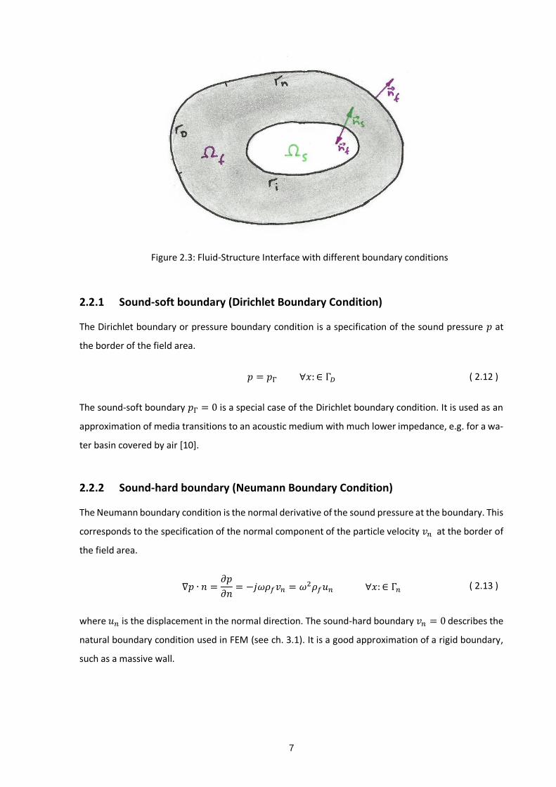
reflecting boundary conditions. Figure 2.3 shows a general example of a fluid-structure interaction
with different boundary conditions applied at the borders.
Figure 2.2: Illustration of sound wave, wave length and period [21]
7
2.2.1 Sound-soft boundary (Dirichlet Boundary Condition)
The Dirichlet boundary or pressure boundary condition is a specification of the sound pressure 𝑝 at
the border of the field area.
𝑝 = 𝑝Γ ∀𝑥: ∈ Γ𝐷 ( 2.12 )
The sound-soft boundary 𝑝Γ = 0 is a special case of the Dirichlet boundary condition. It is used as an
approximation of media transitions to an acoustic medium with much lower impedance, e.g. for a wa-
ter basin covered by air [10].
2.2.2 Sound-hard boundary (Neumann Boundary Condition)
The Neumann boundary condition is the normal derivative of the sound pressure at the boundary. This
corresponds to the specification of the normal component of the particle velocity 𝑣𝑛 at the border of
the field area.
∇𝑝 ∙ 𝑛 =𝜕𝑝
𝜕𝑛= −𝑗𝜔𝜌𝑓𝑣𝑛 = 𝜔2𝜌𝑓𝑢𝑛 ∀𝑥: ∈ Γ𝑛 ( 2.13 )
where 𝑢𝑛 is the displacement in the normal direction. The sound-hard boundary 𝑣𝑛 = 0 describes the
natural boundary condition used in FEM (see ch. 3.1). It is a good approximation of a rigid boundary,
such as a massive wall.
Figure 2.3: Fluid-Structure Interface with different boundary conditions

8
2.2.3 Robin Boundary Condition
For a plane wave the acoustic impedance 𝑍𝑛 is defined by the relationship between the acoustic pres-
sure and the normal component of the particle velocity. It is the resistance of an acoustic medium to
the wave propagation.
𝑍𝑛 =𝑝
𝑣𝑛 ( 2.14 )
with the complex pressure amplitude 𝑝 = 𝑝𝑖𝑛𝑐𝑖𝑑𝑒𝑛𝑡 + 𝑝𝑟𝑒𝑓𝑙𝑒𝑐𝑡𝑒𝑑. At fluid boundaries, the incident
waves are partly absorbed and partly reflected depending on the relation between the specific acoustic
impedances of the acoustic medium and the boundary. The reflection ratio 𝑟𝑟 is a technical measurable
variable [10], which describes the ratio of reflected and incident acoustic pressure waves, it can be
presented by the specific impedances of the regarded acoustic media at the boundary.
𝑟𝑟 =𝑍2 − 𝑍1
𝑍2 + 𝑍1=
|𝑝𝑟|
|𝑝𝑖| ( 2.15 )
Sound-hard boundaries, such as rigid walls, have a reflection ratio 𝑟𝑟 = 1, whereas open domains have
a reflection ratio 𝑟𝑟 = 0 and therefore no reflection at all. Unfortunately, the absence of reflection at
open domains is only true when incoming waves are perpendicular to the surface of the boundary [14].
Figure 2.4 shows the reflection and absorption of an incoming wave at a wall with a rigid boundary as
well as an open domain boundary. Depending on the size of the acoustic domain the reflection rate at
the open domain boundary can be improved.
Figure 2.4: Transmission at a border with impedance boundary condition
9
In the far field pressure and particle velocity are in phase. The relationship can be expressed as
𝑝 = 𝜌0𝑐𝑣𝑛 ( 2.16 )
This leads to the characteristic sound impedance
𝑍0 = 𝜌0𝑐 ( 2.17 )
The admittance boundary is a special case of the Robin boundary condition, which is a weighted com-
bination of the Dirichlet and Neumann boundary condition.
∇𝑝 ∙ 𝑛 =𝜕𝑝
𝜕𝑛= −𝑗𝜔𝜌𝑓(𝑣𝑛,𝑓 − 𝑣𝑛,𝑠) ∀𝑥 ∈ Γ𝑅 ( 2.18 )
with
𝑣𝑛,𝑓 − 𝑣𝑛,𝑠 = 𝐴𝑛𝑝 = 𝑝
𝑍𝑛 ( 2.19 )
where 𝑣𝑛,𝑓 is the normal velocity of the fluid particle on the boundary, 𝑣𝑛,𝑠 is the normal velocity of
the structure surface and 𝐴𝑛 is the normal admittance. Using the Euler equation ( 2.5 ) to change the
particle velocity into pressure shows
∇𝑝 ∙ 𝑛 =𝜕𝑝
𝜕𝑛= −𝑗𝜔𝜌𝑓(𝐴𝑛𝑝 ) = −𝑗𝜔𝜌𝑓 (
𝑝
𝑍𝑛 ) = −
𝜌0
𝑍𝑛
𝜕𝑝
𝜕𝑡 ( 2.20 )
The density 𝜌0 of the fluid can be replaced by the specific sound impedance of the fluid. This yields to
the Robin boundary condition in terms of impedances.
𝜕𝑝
𝜕𝑛= −
𝑍0
𝑍𝑛
1
𝑐
𝜕𝑝
𝜕𝑡= −
1 + 𝑟𝑟
1 − 𝑟𝑟
1
𝑐
𝜕𝑝
𝜕𝑡 ∀𝑥 ∈ Γ𝑖 ( 2.21 )
Setting 𝑍𝑛 = 𝑍0 the radiation boundary condition [11] as a special case of the Robin Boundary Condi-
tion is
𝜕𝑝
𝜕𝑛= −
1
𝑐
𝜕𝑝
𝜕𝑡 ∀𝑥 ∈ Γ𝑟 ( 2.22 )
The radiation boundary is an open domain boundary and therefore shows no reflection at all, if the
incident waves arrive in the normal direction to the boundary. At impedance boundaries, e.g. at the
border of the FSI, the reflection is depending on the impedances of the two acoustic media and can be
described by the reflection ratio.
10
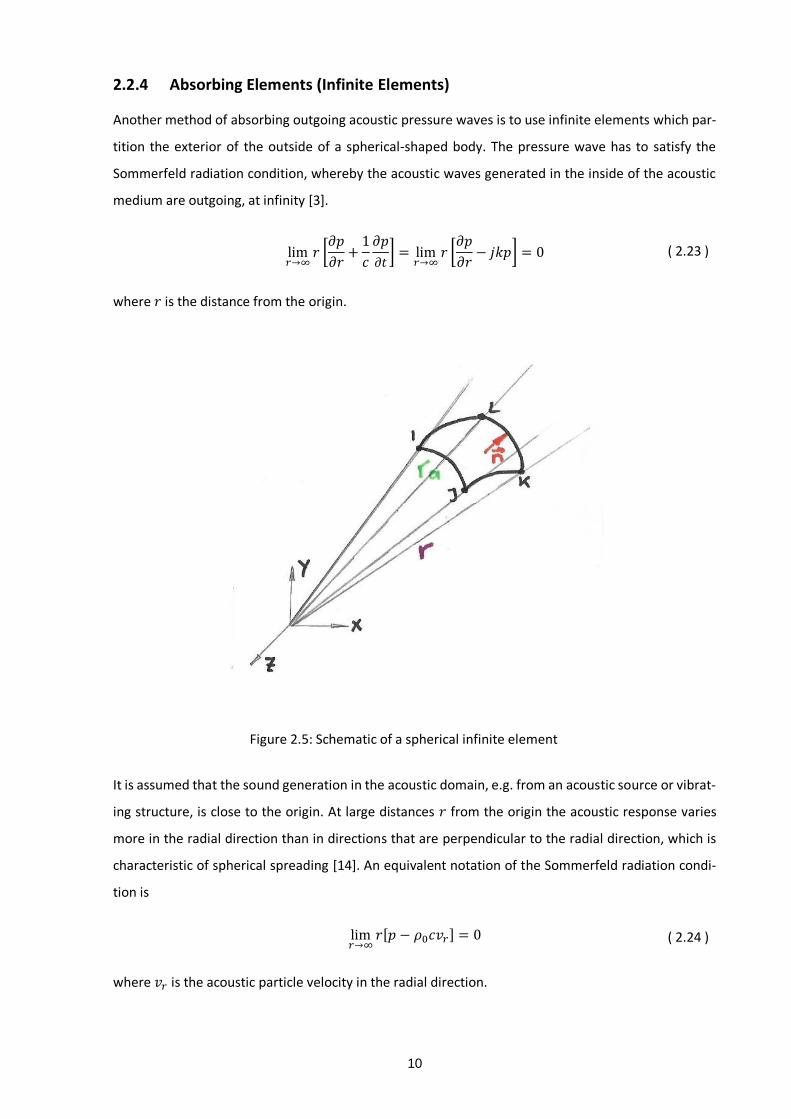
2.2.4 Absorbing Elements (Infinite Elements)
Another method of absorbing outgoing acoustic pressure waves is to use infinite elements which par-
tition the exterior of the outside of a spherical-shaped body. The pressure wave has to satisfy the
Sommerfeld radiation condition, whereby the acoustic waves generated in the inside of the acoustic
medium are outgoing, at infinity [3].
lim𝑟→∞
𝑟 [𝜕𝑝
𝜕𝑟+
1
𝑐
𝜕𝑝
𝜕𝑡] = lim
𝑟→∞𝑟 [
𝜕𝑝
𝜕𝑟− 𝑗𝑘𝑝] = 0 ( 2.23 )
where 𝑟 is the distance from the origin.
It is assumed that the sound generation in the acoustic domain, e.g. from an acoustic source or vibrat-
ing structure, is close to the origin. At large distances 𝑟 from the origin the acoustic response varies
more in the radial direction than in directions that are perpendicular to the radial direction, which is
characteristic of spherical spreading [14]. An equivalent notation of the Sommerfeld radiation condi-
tion is
lim𝑟→∞
𝑟[𝑝 − 𝜌0𝑐𝑣𝑟] = 0 ( 2.24 )
where 𝑣𝑟 is the acoustic particle velocity in the radial direction.
Figure 2.5: Schematic of a spherical infinite element

11
Equation ( 2.24 ) suggests that at large distances 𝑟 → ∞, the acoustic field resembles an outward-
proceeding plane wave [3]. Rearranging this equation leads to the suggestion that at large distances 𝑟,
the acoustic field resembles an outward-travelling plane wave. The impedance can then be described
as
𝑍 =𝑝
𝑣𝑟 ( 2.25 )
While at infinite distances from the origin, the Sommerfeld radiation condition provides perfect ab-
sorption, the boundary condition has to be applied to an external surface of the acoustic domain in a
finite element model [14]. Consequently, appropriate mass, stiffness and damping matrices, which
satisfy the boundary condition (translated into a proper expression for a finite radius 𝑟), have to be
implemented to an element attached to the exterior boundary of the acoustic domain.
2.2.5 Perfectly Matched Layers
Perfectly Matched Layers (PMLs) are artificial anisotropic materials that absorb all incident waves with-
out any reflection, except those that are travelling tangentially to the PML interface [14]. The PML
region acts as an infinite open domain and is attached to the acoustic medium.
Figure 2.6 shows a typical example for the construction of the PML enclosure. It can be seen that all
edges of the bodies align with the coordinate system and a sound-soft Dirichlet boundary is applied on
the border. Those conditions are of technical importance to the computational implementation within
the FEM [3].
Figure 2.6: Construction of the PML
12
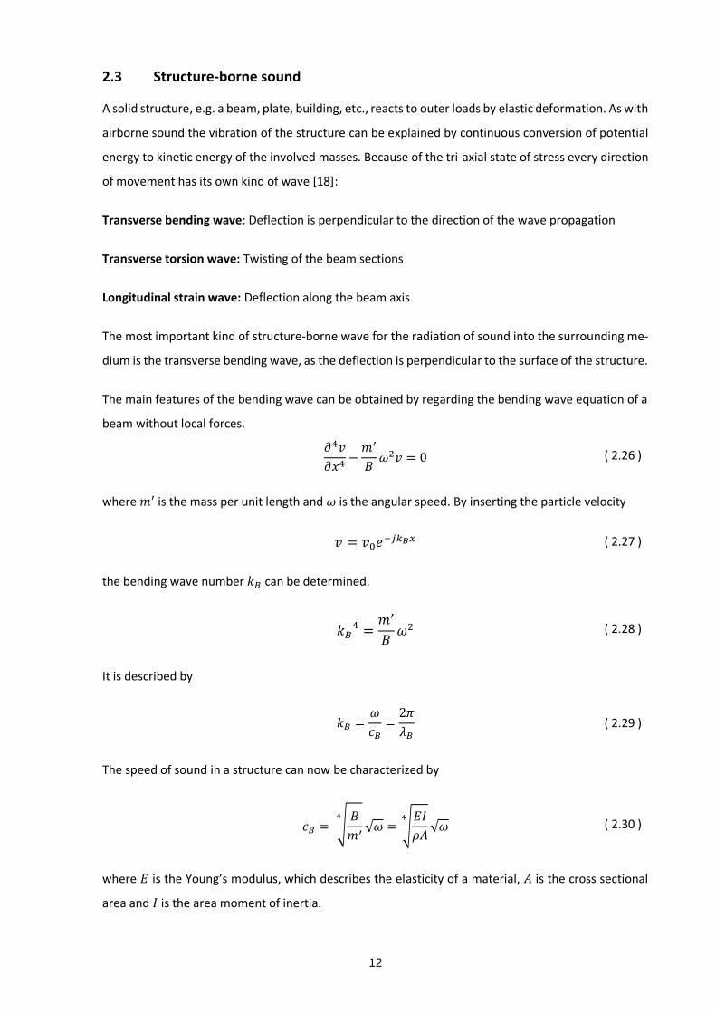
2.3 Structure-borne sound
A solid structure, e.g. a beam, plate, building, etc., reacts to outer loads by elastic deformation. As with
airborne sound the vibration of the structure can be explained by continuous conversion of potential
energy to kinetic energy of the involved masses. Because of the tri-axial state of stress every direction
of movement has its own kind of wave [18]:
Transverse bending wave: Deflection is perpendicular to the direction of the wave propagation
Transverse torsion wave: Twisting of the beam sections
Longitudinal strain wave: Deflection along the beam axis
The most important kind of structure-borne wave for the radiation of sound into the surrounding me-
dium is the transverse bending wave, as the deflection is perpendicular to the surface of the structure.
The main features of the bending wave can be obtained by regarding the bending wave equation of a
beam without local forces.
𝜕4𝑣
𝜕𝑥4−
𝑚′
𝐵𝜔2𝑣 = 0 ( 2.26 )
where 𝑚′ is the mass per unit length and 𝜔 is the angular speed. By inserting the particle velocity
𝑣 = 𝑣0𝑒−𝑗𝑘𝐵𝑥 ( 2.27 )
the bending wave number 𝑘𝐵 can be determined.
𝑘𝐵4 =
𝑚′
𝐵𝜔2 ( 2.28 )
It is described by
𝑘𝐵 =𝜔
𝑐𝐵=
2𝜋
𝜆𝐵 ( 2.29 )
The speed of sound in a structure can now be characterized by
𝑐𝐵 = √
𝐵
𝑚′
4
√𝜔 = √𝐸𝐼
𝜌𝐴
4
√𝜔 ( 2.30 )
where 𝐸 is the Young’s modulus, which describes the elasticity of a material, 𝐴 is the cross sectional
area and 𝐼 is the area moment of inertia.

13
The bending wave length results in
𝜆𝐵 = 2𝜋√
𝐵
𝑚′
4 1
√𝜔= 2𝜋√
𝐸𝐼
𝜌𝐴
4 1
√𝜔 ( 2.31 )
In contrast to airborne sound, the wave of wave length 𝜆𝐵 has a frequency depending speed of sound
𝑐𝐵. Similar to the bending wave of a beam, the bending wave length for a homogeneous plate can be
written as
𝜆𝐵 = 2𝜋√
𝐵′
𝑚′′
4 1
√𝜔 ( 2.32 )
with
𝐵′ =𝐸
1 − 𝜇2
ℎ3
12 ( 2.33 )
and
𝑚′′ = 𝜌ℎ ( 2.34 )
where 𝑚′′ is the area density, 𝐵′ is the bending resistance of the plate, ℎ is the thickness of the plate
and 𝜇 is the Poisson’s ratio.
Neglecting 𝜇2 ≪ 1 the quotient 𝐵′
𝑚′′ can be simplified to
𝐵′
𝑚′′= 12
𝜌ℎ
𝐸ℎ3=
12
𝑐𝐿2ℎ2
( 2.35 )
where 𝑐𝐿 = √𝐸
𝜌 is the speed of the longitudinal wave. The bending wave length can then be approxi-
mated to
𝜆𝐵 ≈ 1.35√
ℎ𝑐𝐿
𝑓 ( 2.36 )
and the structure-borne speed of sound to
𝑐𝐵 ≈ 1.35√ℎ𝑐𝐿𝑓 ( 2.37 )
14
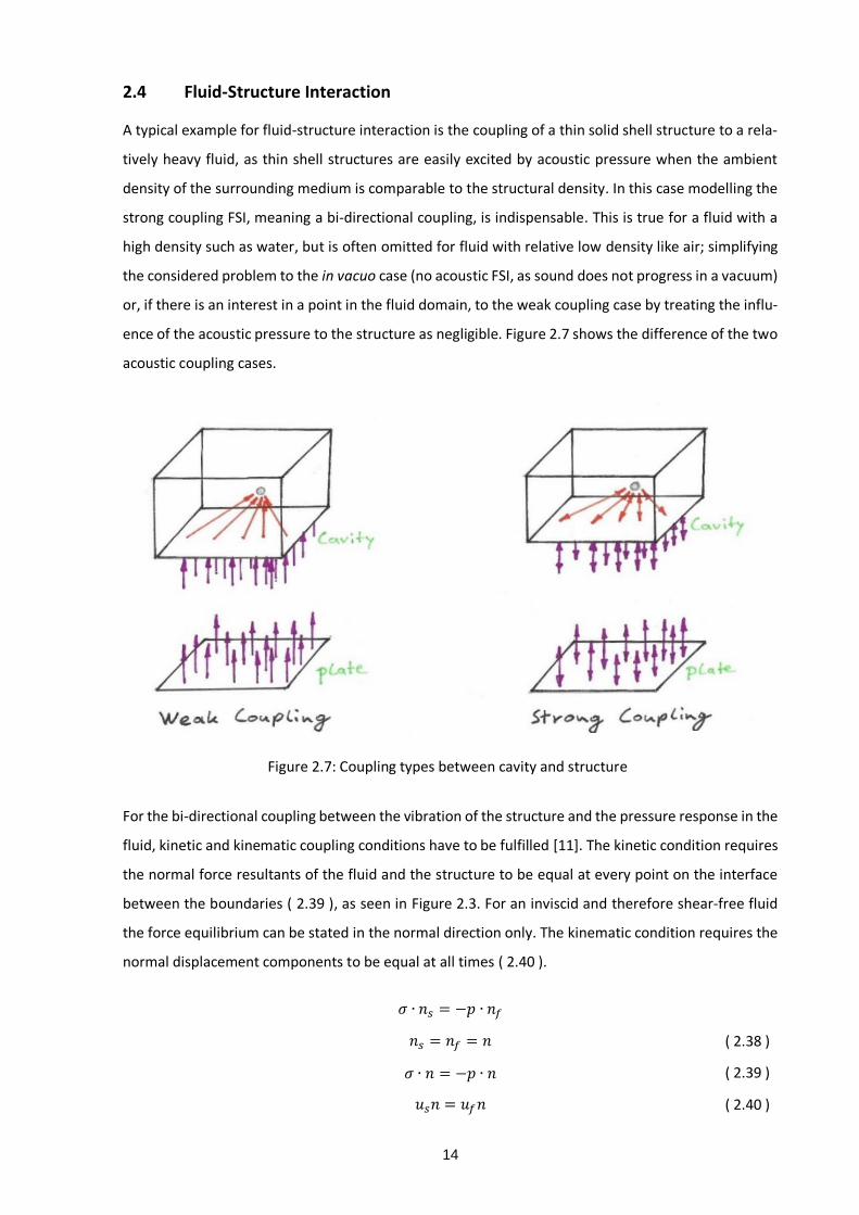
2.4 Fluid-Structure Interaction
A typical example for fluid-structure interaction is the coupling of a thin solid shell structure to a rela-
tively heavy fluid, as thin shell structures are easily excited by acoustic pressure when the ambient
density of the surrounding medium is comparable to the structural density. In this case modelling the
strong coupling FSI, meaning a bi-directional coupling, is indispensable. This is true for a fluid with a
high density such as water, but is often omitted for fluid with relative low density like air; simplifying
the considered problem to the in vacuo case (no acoustic FSI, as sound does not progress in a vacuum)
or, if there is an interest in a point in the fluid domain, to the weak coupling case by treating the influ-
ence of the acoustic pressure to the structure as negligible. Figure 2.7 shows the difference of the two
acoustic coupling cases.
For the bi-directional coupling between the vibration of the structure and the pressure response in the
fluid, kinetic and kinematic coupling conditions have to be fulfilled [11]. The kinetic condition requires
the normal force resultants of the fluid and the structure to be equal at every point on the interface
between the boundaries ( 2.39 ), as seen in Figure 2.3. For an inviscid and therefore shear-free fluid
the force equilibrium can be stated in the normal direction only. The kinematic condition requires the
normal displacement components to be equal at all times ( 2.40 ).
𝜎 ∙ 𝑛𝑠 = −𝑝 ∙ 𝑛𝑓
𝑛𝑠 = 𝑛𝑓 = 𝑛 ( 2.38 )
𝜎 ∙ 𝑛 = −𝑝 ∙ 𝑛 ( 2.39 )
𝑢𝑠𝑛 = 𝑢𝑓𝑛 ( 2.40 )
Figure 2.7: Coupling types between cavity and structure

15
2.5 Perception of Sound
The human ear is a highly sensitive receiver capable of perceiving sound waves with frequencies be-
tween 16 Hz and 20 kHz [8]. The limits of, in the field of vibro-acoustic interested, audible sound are
not sharply specified, as the upper limits vary individually depending on the age of a person and other
factors, such as noise exposure at work or habitual exposure to loud music [18].
Sound events with the same sound pressure but a different frequency are not considered equal in
loudness. In order to evaluate the subjective effect of a sound event it is not enough to specify the
objectively measurable sound pressure, rather the frequency-dependent sense of hearing must be
considered [16]. The definition of volume is based on the subjective comparison of a sound event with
the reference sound pressure 𝑝0 = 2 ∙ 10−5𝑃𝑎 of an incident plane wave with the frequency of
1000 Hz.
This leads to the sound pressure level (SPL)
𝐿𝑖 = 20 log (𝑝
𝑝0) = 10 log (
𝑝
𝑝0)2
( 2.41 )
The perceived volume of a sound with the same loudness as a pure tone has the SPL 𝐿 with its own
unit called phon. At the frequency of 1000 Hz the values for volume and SPL are identical. Measure-
ments of pure tones depending on the frequency follows the curves of equal loudness found in Figure
2.8.
Figure 2.8: Fletcher-Munson curves of equal loudness [20]
16
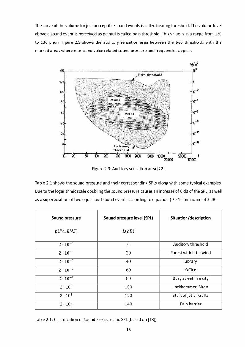
The curve of the volume for just perceptible sound events is called hearing threshold. The volume level
above a sound event is perceived as painful is called pain threshold. This value is in a range from 120
to 130 phon. Figure 2.9 shows the auditory sensation area between the two thresholds with the
marked areas where music and voice related sound pressure and frequencies appear.
Table 2.1 shows the sound pressure and their corresponding SPLs along with some typical examples.
Due to the logarithmic scale doubling the sound pressure causes an increase of 6 dB of the SPL, as well
as a superposition of two equal loud sound events according to equation ( 2.41 ) an incline of 3 dB.
Sound pressure
𝑝(𝑃𝑎, 𝑅𝑀𝑆)
Sound pressure level (SPL)
𝐿(𝑑𝐵)
Situation/description
2 ∙ 10−5 0 Auditory threshold
2 ∙ 10−4 20 Forest with little wind
2 ∙ 10−3 40 Library
2 ∙ 10−2 60 Office
2 ∙ 10−1 80 Busy street in a city
2 ∙ 100 100 Jackhammer, Siren
2 ∙ 101 120 Start of jet aircrafts
2 ∙ 102 140 Pain barrier
Figure 2.9: Auditory sensation area [22]
Table 2.1: Classification of Sound Pressure and SPL (based on [18])

17
The total SPL can be calculated with
𝐿𝑡 = 10 log (∑10𝐿𝑖/10
𝑛
𝑖=1
) ( 2.42 )
To represent the sensitivity of the human ear the sound level in the measurement and evaluation is
often filtered. This reduces the weighting of the low frequencies and enhances the mid frequencies.
Very often the A-filtered SPL is used, as it most resembles the human auditory sensation.
𝐿(𝐴) = 10 log (∑10(𝐿𝑖+∆𝑖)/10
𝑛
𝑖=1
) ( 2.43 )
where ∆𝑖 is an attenuation factor according to the weighting in Figure 2.10.
Figure 2.10: A-,B-,C- weighted filter curves [22]
18
3 Finite Element Analysis
The finite element analysis (FEA) is a numerical method for finding approximate solutions to boundary
value problems for partial differential equations. It can be used to calculate the response of a model
by applying forcing functions, e.g. an acoustic source or mechanical forces. The to be analysed domain,
e.g. a solid, a structure, a fluid, or a coupled fluid structure, is therefore partitioned into subdomains
called finite elements whose corner points are called nodes.
In case of the fluid-structure interaction the physical unknowns 𝑢 and 𝑝 are approximated by nodal
functions 𝑢ℎ ≈ 𝑢, 𝑝ℎ ≈ 𝑝
𝑢ℎ(𝑥, 𝑡) = ∑𝑢𝑖(𝑡)
𝑛𝑠
𝑖=1
𝜑𝑖(𝑥), 𝑝ℎ(𝑥, 𝑡) = ∑ 𝑝𝑖
𝑛𝑓
𝑖=1
(𝑡) 𝜑𝑖(𝑥) ( 3.1 )
where 𝑢𝑖, 𝑝𝑖 are unknown nodal values, 𝑛𝑠 is the number of nodes of the solid domain, 𝑛𝑓 is the num-
ber of nodes of the fluid domain and 𝜑𝑖 are linear interpolants called testing functions. The summation
extends over all nodes in the solid and fluid domain, separately for each one.
3.1 Governing Equations
The FE discretization procedure starts from the weak formulation of the partial differential equation
(PDE). This formulation can be obtained by testing the PDEs using the Galerkin procedure. After the
discretization of the weak formulations the coupling of the fluid and structure will be created.
3.1.1 Derivation of the variational formulations
For the finite element formulation of the acoustic fluid the Helmholtz equation ( 2.9 ) is multiplied by
a testing function 𝑤 and integrated over the computational domain 𝛺𝑓, whereby the stationary vector
function 𝑤 satisfies the Dirichlet boundary condition.
∫ 𝑤(∇ ∙ (∇𝑝) + 𝑘2𝑝)𝛺𝑓
𝑑𝑉 = 0 ( 3.2 )
∫ 𝑤 ∙ ∇ ∙ (∇𝑝) 𝑑𝑉 + ∫ 𝑤 ∙ 𝑘2𝑝
𝛺𝑓𝛺𝑓
𝑑𝑉 = 0
Using the Gauss integral theorem to integrate the first term yields the weak formulation
∫ ∇𝑤 ∙ ∇𝑝 𝑑𝑉 − ∫ 𝑤 ∇𝑝 ∙ 𝑛 𝑑𝐴
𝛤
− ∫ 𝑤 ∙ 𝑘2𝑝𝛺𝑓𝛺𝑓
𝑑𝑉 = 0 ( 3.3 )

19
Rearranging and simplifying to
∫ ∇𝑤 ∙ ∇𝑝 𝑑𝑉 − ∫ 𝑤 ∙ 𝑘2𝑝
𝛺𝑓𝛺𝑓
𝑑𝑉 = ∫ 𝑤 𝜕𝑝
𝜕𝑛 𝑑𝐴 = −
𝛤
∫ 𝑗𝑤𝜔𝜌𝑓𝑣𝑛𝑑𝐴𝛤
( 3.4 )
Applying the natural boundary condition in FEM by setting a sound-hard boundary will simplify the
term to
∫ ∇𝑤 ∙ ∇𝑝 𝑑𝑉 − ∫ 𝑤 ∙ 𝑘2𝑝
𝛺𝛺
𝑑𝑉 = 0 ( 3.5 )
Similar to the acoustic fluid the weak formulation of the structural vibration can be gathered by using
the equilibrium ( 2.4 ) in terms of 𝜎 and expand it into three dimensions. Multiplying this equilibrium
by a stationary vector function 𝑞 and integrating it over the solid domain 𝛺𝑠 equates
−∫ ∇σ ∙ q 𝑑𝑉 + ∫ 𝜌𝑠�̈�
𝛺
∙ q 𝑑𝑉𝛺
= 0 ( 3.6 )
The weak formulation is gained by using the Gauss integral theorem to integrate the first term by parts
∫ σ: ∇q 𝑑𝑉 − ∫ (𝜎 ∙ 𝑛) ∙ 𝑞 𝑑𝐴
𝛤
∫ 𝜌𝑠�̈�𝛺
∙ q 𝑑𝑉𝛺
= 0 ( 3.7 )
With 𝜎 = 𝐶휀 = 𝐶𝐷𝑢, where 𝐶 is the solid material tensor and 𝐷 is the operator matrix
𝐷 =
[ 𝜕
𝜕𝑥0 0
0𝜕
𝜕𝑦0
0 0𝜕
𝜕𝑧𝜕
𝜕𝑦
𝜕
𝜕𝑥0
𝜕
𝜕𝑧0
𝜕
𝜕𝑥
0𝜕
𝜕𝑧
𝜕
𝜕𝑦]
( 3.8 )
and 휀(𝑞) = 𝐷𝑞 the tensor scalar σ: ∇q = σ(𝑢): 휀(𝑞) can be written as σ: ∇q = (𝐷𝑞)𝑇𝐶(𝐷𝑢), so that
∫ (𝐷𝑞)𝑇𝐶(𝐷𝑢) 𝑑𝑉 − ∫ (𝜎 ∙ 𝑛) ∙ 𝑞 𝑑𝐴
𝛤
∫ 𝜌𝑠�̈�𝛺
∙ q 𝑑𝑉𝛺
= 0 ( 3.9 )
20
3.1.2 Derivation of the Discrete Systems
The FEA is based on the discretisation of the weak form. The regarded system is divided into a number
of elements with 𝑛 nodes. The acoustic pressure and weighting function 𝑤 can be approximated by
using the Galerkin method to
𝑝 = ∑𝜑𝑖 𝑝𝑖
𝑛
𝑖=1
( 3.10 )
𝑤 = ∑𝜑𝑗𝑤𝑗
𝑛
𝑗=1
( 3.11 )
where 𝜑𝑖 are test functions. By inserting equation ( 3.10 ) and ( 3.11 ) the weak form ( 3.4 ) can be
written as
𝑤𝑖 ∫ ∇𝜑𝑖∇𝜑𝑗 𝑑𝑉 𝑝𝑗 − 𝑘2𝑤𝑖 ∫ 𝜑𝑖𝜑𝑗 𝑑𝑉 𝑝𝑗
𝛺𝑓𝛺𝑓
= 𝑗𝜌𝑓𝑤𝑖𝜔 ∫ 𝜑𝑖𝜑𝑗𝑣𝑛𝑑𝐴𝛤
( 3.12 )
for every combination of 𝑖 and 𝑗 within an element [10]. Replacing 𝑘 by equation ( 2.10 ) equals
𝑤𝑖 ∫ ∇𝜑𝑖∇𝜑𝑗 𝑑𝑉 𝑝𝑗 −
𝜔2
𝑐2𝑤𝑖 ∫ 𝜑𝑖𝜑𝑗 𝑑𝑉 𝑝𝑗
𝛺𝑓𝛺𝑓
= 𝑗𝜌𝑓𝑤𝑖𝜔 ∫ 𝜑𝑖𝜑𝑗𝑣𝑛𝑑𝐴𝛤
( 3.13 )
With 𝑤𝑖 = 1 and by introducing [𝑀𝑓] = 1
𝑐2 ∫ 𝜑𝑖𝜑𝑗 𝑑𝑉𝛺𝑓
as the mass matrix, [𝐾𝑓] = ∫ ∇𝜑𝑖∇𝜑𝑗 𝑑𝑉𝛺𝑓
as
the stiffness matrix, and {𝐹𝑓} = 𝑗𝜌𝑓𝜔∫ 𝜑𝑖𝜑𝑗𝑣𝑛𝑑𝐴𝛤
= 𝜌𝑓𝜔2 ∫ 𝜑𝑖𝜑𝑗𝑑𝐴 𝑢𝑛𝛤
as the load vector of the
discrete system, the discretised system can be written as
(−𝜔2[𝑀𝑓] + [𝐾𝑓]){𝑝} = {𝐹𝑓} ( 3.14 )
By introducing the impedance boundary condition the discrete system of equation ( 3.13 ) is
𝑤𝑖 ∫ ∇𝜑𝑖∇𝜑𝑗 𝑑𝑉 𝑝𝑗 −𝜔2
𝑐2𝑤𝑖 ∫ 𝜑𝑖𝜑𝑗 𝑑𝑉 𝑝𝑗 +
𝛺𝑓𝛺𝑓
𝑗𝜔𝜌𝑓𝑤𝑖 ∫ 𝜑𝑖𝜑𝑗
1
𝑍𝑛,𝑗𝑑𝐴 𝑝𝑗
𝛤𝑖
= 𝜌𝑓𝑤𝑖𝜔2 ∫ 𝜑𝑖𝜑𝑗𝑑𝐴
𝛤𝑛
𝑢𝑛
( 3.15 )
where 𝛤𝑛 is the border of the Neumann boundary and 𝛤𝑖 is the border of the impedance boundary.

21
Equation ( 3.14 ) can now be expressed as
(−𝜔2[𝑀𝑓] + 𝑗𝜔[𝐶𝑓] + [𝐾𝑓]){𝑝} = {𝐹𝑓} ( 3.16 )
where [𝐶𝑓] = 𝜌𝑓 ∫ 𝜑𝑖𝜑𝑗1
𝑍𝑛,𝑗𝑑𝐴
𝛤𝑖 is the damping matrix of the fluid.
Similar to the acoustic fluid the discretised system of the structure can be written as
(−𝜔2[𝑀𝑠] + 𝑗𝜔[𝐶𝑠] + [𝐾𝐹]){𝑢} = {𝐹𝑠} ( 3.17 )
where [𝑀𝑠] = 𝜌 ∫ 𝜑𝑖𝜑𝑗 𝑑𝑉𝛺𝑠
is the mass matrix and [𝐾𝑠] = ∫ 𝜑𝑖𝐷𝑇𝐶𝐷𝜑𝑗 𝑑𝑉
𝛺𝑠 is the stiffness matrix.
The load vector {𝐹𝑠} = [𝑇𝑠]{𝑓} + [𝐺𝑆]{𝑡} consists of the interpolation matrices [𝑇𝑠] = ∫ 𝜑𝑖𝜑𝑗 𝑑𝑉𝛺𝑠
for
the inner forces and [𝐺𝑠]=∫ 𝜑𝑖𝜑𝑗 𝑑𝐴𝛤
for the outer forces, where {𝑓} is the vector of the volume forces
and {𝑡} is the vector of the surface loads [10]. The structural damping can be respected by the propor-
tional damping matrix [𝐶𝑠] = 𝛼[𝑀𝑠] + 𝛽[𝐾𝑠] with 𝛼 and 𝛽 as damping parameters.
3.1.3 Implementation of the FSI
Applying the coupling conditions ( 2.39 ) and ( 2.40 ) to the discretised weak formulations of the equa-
tions of motion for the structure and fluid equals
(−𝜔2[𝑀𝑠] + 𝑗𝜔[𝐶𝑠] + [𝐾𝐹]){𝑢} − [𝑅]{𝑝} = {𝐹𝑠} ( 3.18 )
(−𝜔2[𝑀𝑓] + 𝑗𝜔[𝐶𝑓] + [𝐾𝑓]){𝑝} − 𝜔2𝜌0[𝑅]𝑇{𝑢} = {𝐹𝑓} ( 3.19 )
with 𝑝 = 𝜔2𝜌0𝑢, where [𝑅] is the coupling matrix that take in account the surface area associated
with each node on the fluid-structure interface. Written down as a linear system it is shown that the
dynamic stiffness matrix is not symmetric.
(−𝜔2 [𝑀𝑆 0
𝜌0𝑅𝑇 𝑀𝐹
] + 𝑗𝜔 [𝐶𝑆 00 𝐶𝐹
] + [𝐾𝑆 −𝑅0 𝐾𝐹
]) {𝑢𝑝} = {
𝐹𝑠
𝐹𝑓} ( 3.20 )
By defying a transformation variable for the nodal pressure ( 3.21 ) the symmetric formulation of the
linear system ( 3.22 ) can be obtained [4].
�̇� = 𝑗𝜔𝑞 = 𝑝 ( 3.21 )
(−𝜔2 [
𝑀𝑆 0
0 −𝑀𝐹
𝜌0
] + 𝐽𝜔 [
𝐶𝑆 −𝑅
−𝑅𝑇 −𝐶𝐹
𝜌0
] + [
𝐾𝑆 0
0 −𝐾𝐹
𝜌0
]) {𝑢𝑞} = {
𝐹𝑠
𝑗
𝜔𝜌0𝐹𝑓
} ( 3.22 )
22
3.2 Solution Methods for Frequency Response
While looking at the response of a vibrating system the frequency response is more of interest than its
behaviour in time, as it clearly indicates the eigenfrequencies of a system and its response to it. The
frequency response therefore records the magnitude and phase of the vibrating system as a function
of frequency, e.g. in this work the frequency response of the amplitude of displacement or acoustic
pressure is used to describe the behaviour of the system.
The solution used in the frequency response can be gained by the direct solution of the discrete system
or the mode superposition method.
3.2.1 Direct Solution
The direct solution can be obtained by calculating the displacement and acoustic pressure of the linear
system ( 3.20 ) or the symmetric equivalent ( 3.22 ) for every defined forcing frequency 𝛺 within the
requested frequency range [𝛺𝑚𝑖𝑛 : 𝛺𝑚𝑎𝑥] [11].
Therefore, the displacement and acoustic pressure of the discrete system
(−𝛺2[𝑀] + 𝑖𝛺[𝐶] + [𝐾]){𝑢} = {𝑓} ( 3.23 )
can be computed by multiplying the inverse of the dynamic stiffness matrix on the left side with the
force vector {𝑓}.
{𝑢} = [−𝛺2[𝑀] + 𝑗𝛺[𝐶] + [𝐾]]−1
{𝑓} ( 3.24 )
Because of the dependency of the forcing frequency 𝜔, the inverse of the dynamic stiffness matrix has
to be calculated at every sub-step. This leads to high computing times depending on the system’s DOFs
as well as the requested frequency range.
3.2.2 Mode Superposition
As an alternative to the direct approach, the solution of the harmonic response can be obtained by
modal superposition. In a first step the natural frequencies and mode shapes are obtained from a
modal analysis, which later characterises the dynamic response of the steady harmonic excitation [2].
The frequency response solution is searched as a superposition of eigenvectors 𝛷𝑖. {𝑢} is
{𝑢} = ∑{𝛷𝑖}
𝑁
𝑖=1
𝑦𝑖 ( 3.25 )
23
where 𝑁 is the number of modes used in the computation and 𝑦𝑖 are modal coordinates of the real
valued eigenvectors of the form 𝛷 = {𝑢}, and 𝛷 = {𝑢𝑝} for the coupled problem respectively. With
𝑁 ≪ 𝑛, the solution will be searched in form of the lower eigenvectors’ superposition, whereby 𝑛 rep-
resents the system’s number of modes.
Equation ( 3.23 ) can then be represented as
[𝑀]∑{𝛷𝑖}
𝑁
𝑖=1
�̈�𝑖 + [𝐶]∑{𝛷𝑖}
𝑁
𝑖=1
�̇�𝑖 + [𝐾]∑{𝛷𝑖}
𝑁
𝑖=1
𝑦𝑖 = {𝑓} ( 3.26 )
and by pre-multiplying with the mode shape {𝛷𝑗}𝑇
as
{𝛷𝑗}
𝑇[𝑀]∑{𝛷𝑖}
𝑁
𝑖=1
�̈�𝑖 + {𝛷𝑗}𝑇[𝐶]∑{𝛷𝑖}
𝑁
𝑖=1
�̇�𝑖 + {𝛷𝑗}𝑇[𝐾]∑{𝛷𝑖}
𝑁
𝑖=1
𝑦𝑖 = {𝛷𝑗}𝑇{𝑓} ( 3.27 )
The orthogonality condition of the natural modes states that for 𝑖 ≠ 𝑗
{𝛷𝑗}𝑇[𝑀]{𝛷𝑖} = 0
( 3.28 )
{𝛷𝑗}𝑇[𝐾]{𝛷𝑖} = 0
( 3.29 )
and
{𝛷𝑗}𝑇[𝐶]{𝛷𝑖} = 0 ( 3.30 )
if only Rayleigh or constant damping is allowed. Applying condition ( 3.28 ), ( 3.29 ) and ( 3.30 ) to
equation ( 3.27 ) equals for 𝑖 = 𝑗.
{𝛷𝑗}𝑇[𝑀]{𝛷𝑗} �̈�𝑗 + {𝛷𝑗}
𝑇[𝐶]{𝛷𝑗} �̇�𝑗 + {𝛷𝑗}
𝑇[𝐾]{𝛷𝑗} 𝑦𝑗 = {𝛷𝑗}
𝑇{𝑓} ( 3.31 )
With the modal transformations of the mass and stiffness matrices
[�̂�] = {𝛷𝑗}
𝑇[𝑀]{𝛷𝑗} = [𝐸] = [
1⋱
1
]
𝑁𝑥𝑁
( 3.32 )
[�̂�] = {𝛷𝑗}𝑇[𝐾]{𝛷𝑗} = [𝜔2] = [
𝜔12
⋱𝜔𝑁
2
]
𝑁𝑥𝑁
( 3.33 )

24
equation ( 3.31 ) can be written as
(−𝛺2[�̂�] + 𝑗𝛺{𝛷𝑗}𝑇[𝐶]{𝛷𝑗} + [�̂�]) 𝑦𝑗 = {𝛷𝑗}
𝑇{𝑓} ( 3.34 )
(−𝛺2[𝐸] + 𝑗𝛺{𝛷𝑗}𝑇[𝐶]{𝛷𝑗} + [𝜔2]) 𝑦𝑗 = {𝛷𝑗}
𝑇{𝑓}
By multiplying the inverse of the modal transformed dynamic stiffness matrix on the left side with the
modal transformed force vector {𝑓} the modal coordinates 𝑦𝑗 can be estimated
𝑦𝑗 = (−𝜔2[�̂�] + 𝑗𝜔[�̂�] + [�̂�])−1
{𝑓} ( 3.35 )
The modal coordinates 𝑦𝑗 are then converted back into the geometric displacements {𝑢} by equation
( 3.25 ). For an accurate analysis of the driving frequency belt 𝛺 ∈ [𝛺𝑚𝑖𝑛: 𝛺𝑚𝑎𝑥] the solution should
cover all modes with the associated frequencies 𝜔 ≤ 1.5 ∙ 𝛺𝑚𝑎𝑥 , as they characterise the frequency
response [12]. The approximate solution generally shows a good convergence to the direct solution
within the lower frequencies of the frequency belt. By increasing the number of modes 𝑁 to the sys-
tem’s number of modes 𝑛 the approximate solution equals the modal transformation of the direct
solution. The main advantage of this approach lies within the reduced computational effort, as the
system of equations is consistently trimmed with 𝑁 ≪ 𝑛.
For the mode-superposition in fluid-structure interaction, the symmetric formulation as shown above
may not succeed in extracting all eigensolutions, therefore the unsymmetric formulation along with
the unsymmetric eigensolver is being used [7].
Equation ( 3.31 ) is then replaced by
{𝛷𝑗𝐿}
𝑇[𝑀]{𝛷𝑗}�̈�𝑗 + {𝛷𝑗
𝐿}𝑇[𝐶]{𝛷𝑗}�̇�𝑗 + {𝛷𝑗
𝐿}𝑇[𝐾]{𝛷𝑗}𝑦𝑗 = {𝛷𝑗
𝐿}𝑇{𝑓} ( 3.36 )
where {𝛷𝑗𝐿} is the left mode shape of mode 𝑗 and {𝛷𝑗} is the right mode shape of mode 𝑗.
Residual Vectors
When the applied loads excite the higher frequency modes of a structure the modally truncated solu-
tion will be imprecise. To improve the accuracy of the response additional modal transformation fac-
tors, called residual vectors, can be used [2]. The dynamic response 𝑥 can then be gained by superpo-
sition of the lower mode contributions 𝑥𝐿 by equation ( 3.1 ) and the higher mode contributions 𝑥𝐻,
which can be represented as the combination of residual vectors.
{𝑥} = {𝑥𝐿} + {𝑥𝐻} ( 3.37 )

25
The residual vectors {𝑅} can be expressed as
{𝑅} = [�̃�]{𝑓} ( 3.38 )
with the residual flexibility matrix
[�̃�] = ∑
{𝛷𝑗𝐿}{𝛷𝑗}
𝑇
𝜔𝑗2
𝑛
𝑖=𝑚+1
= [𝐺] − ∑{𝛷𝑗
𝐿}{𝛷𝑗}𝑇
𝜔𝑗2
𝑚
𝑖=1
( 3.39 )
where [𝐺] is the inverse matrix of the stiffness matrix [𝐾]
[𝐺] = ∑
{𝛷𝑗𝐿}{𝛷𝑗}
𝑇
𝜔𝑗2
𝑛
𝑖=1
= ∑{𝛷𝑗
𝐿}{𝛷𝑗}𝑇
𝜔𝑗2
𝑚
𝑖=1
+ ∑{𝛷𝑗
𝐿}{𝛷𝑗}𝑇
𝜔𝑗2
𝑛
𝑖=𝑚+1
( 3.40 )
Restrictions of the Mode Superposition Method
The mode superposition method is not supported if damping, apart from modal damping, proportional
or Rayleigh damping is present [7]. In particular, if acoustic damped boundary conditions, fluid dynam-
ics viscosity, perforated material, PML absorbing condition or infinite elements are defined. Conse-
quently, absorbing boundary conditions are not supported in general.
3.3 Finite Elements for FSI (3D)
In order to solve a FSI problem the fluid and solid volumes are partitioned into finite elements. In case
of the fluid the volume is divided into hexahedral or tetrahedral elements with one degree of freedom
(DOF) per node. The solid domain can be meshed by volume elements with three DOFs or shell ele-
ments with 6 DOFs per knot. For the coupling between solid and fluid elements optional DOFs (corre-
sponding to the translational DOFs of the structure) are being used within the fluid elements (for fur-
ther information see ch. 8.1.2 or [5] and [6]).
Figure 3.1: Hexahedral solid, shell and fluid element with nodal DOFs

26
4 Verification Examples
4.1 Rectangular Panel Backed on Closed Cavity
To demonstrate and validate the structural-acoustical coupling of the FSI between an acoustic medium
and a structure it is common to take a look at a rectangular panel backed by a rectangular closed cavity,
as it represents a typical sound radiating application where the response of a structure is influenced
by the acoustic pressure on its surface and vice versa, e.g. thin walls in frame buildings or machine
housings.
In this example the flexible plate is forced to swing at the point (0.2, 0.3) m due to a time-harmonic
force of 1N within the frequency range Ω = [0: 250]𝑠−1. The elastic panel has the dimensions
1𝑚 ∙ 1𝑚 and the thickness ℎ = 0.01 𝑚. The panel is simply supported and coupled to an acoustic
cavity with the dimensions 1𝑚 ∙ 1𝑚 ∙ 1𝑚. The remaining surfaces of the cavity are rigid walls, i.e. Neu-
mann boundary conditions are applied. The acoustic fluid is water (𝜌𝐹 = 1000𝑘𝑔
𝑚3 , 𝑐𝐹 = 1481𝑚
𝑠) and
the flexible plate is made from steel (𝐸 = 210 𝐺𝑃𝑎, 𝜌𝑆 = 7900𝑘𝑔
𝑚3 , 𝜈 = 0.3).
The frequency response at the driving point is recorded and then compared with the work of M. Fischer
and L. Gaul [17]. The flexible plate’s applied mesh of the referred work consists of 20 ∙ 20 shell ele-
ments with an element length ℎ𝜆 = 0.05𝑚. The same element length is applied to the acoustic cavity.
Figure 4.1: A closed acoustic cavity with an attached flexible plate
27
With the longitudinal speed of sound 𝑐𝐿 and the dominant driving frequency Ω the bending wave
length can be determined
𝑐𝐿 = √𝐸
𝜌= √
210 ∙ 109 𝑁𝑚2
7900𝑘𝑔𝑚3
= 5155.80𝑚
𝑠
𝜆𝐵 ≈ 1.35√
ℎ𝑐𝐿
Ω= 1.35√
0.01𝑚 ∙ 5155.80𝑚𝑠
250 𝑠−1= 0.61𝑚
With the element per wave length condition 𝜆𝐵
ℎ𝜆= 6…8 the recommended element size can be esti-
mated to
ℎ𝜆 =𝜆
8=
0.61𝑚
8= 0.076𝑚 ( 4.1 )
The chosen element length in the referred work ℎ𝜆,𝑐ℎ𝑜𝑠𝑒𝑛 = 0.05𝑚 does fulfil the recommended ele-
ment per wave length condition in equation ( 4.1 ).
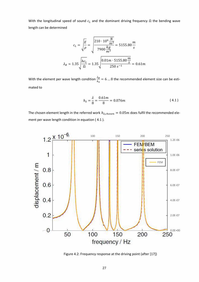
Figure 4.2: Frequency response at the driving point (after [17])
0.0E+00
2.0E-07
4.0E-07
6.0E-07
8.0E-07
1.0E-06
1.2E-06
0 50 100 150 200 250
FEM
28
The frequency response of the graph in Figure 4.2 compares the FEM solution of ANSYS with the ana-
lytical Fourier series solution derived by Pretlove [1] and the FEM-BEM solution by M. Fischer and L.
Gaul. All graphs show an appropriate correspondence to each other.
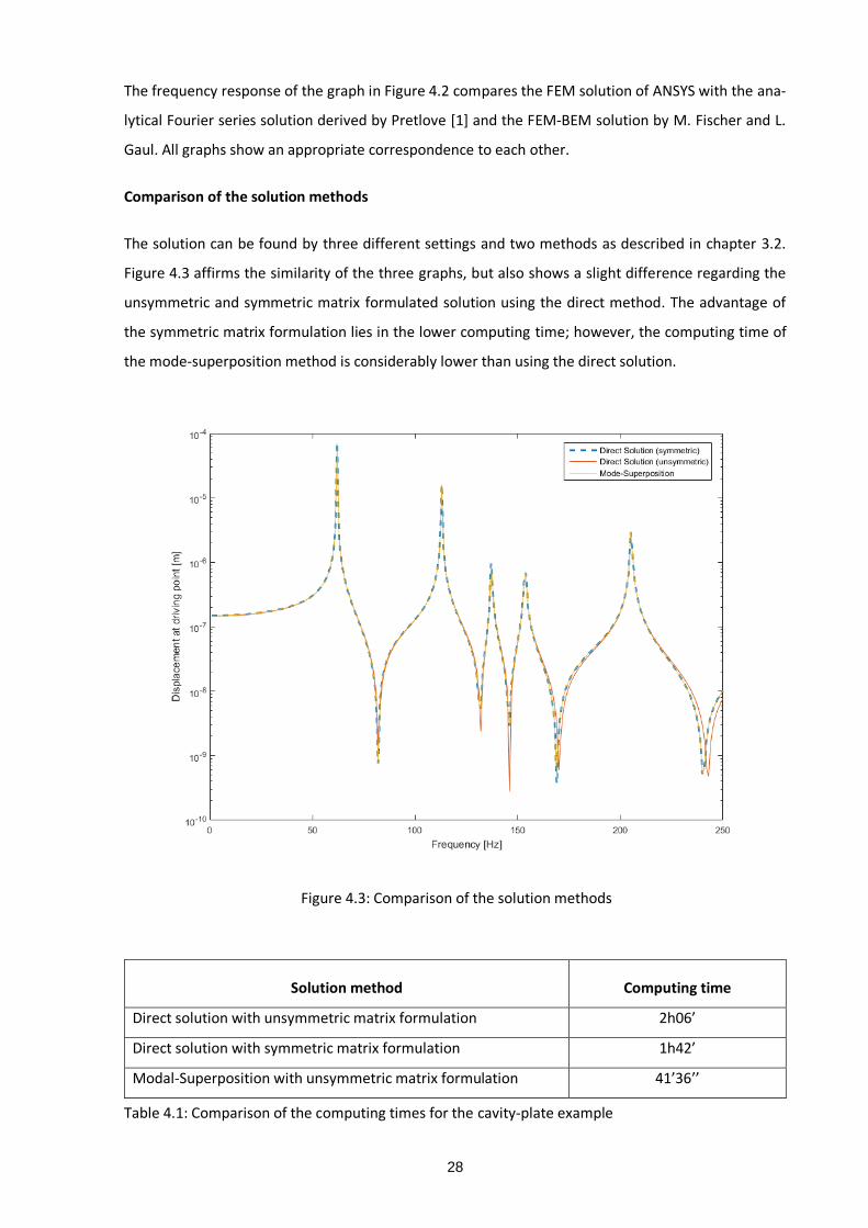
Comparison of the solution methods
The solution can be found by three different settings and two methods as described in chapter 3.2.
Figure 4.3 affirms the similarity of the three graphs, but also shows a slight difference regarding the
unsymmetric and symmetric matrix formulated solution using the direct method. The advantage of
the symmetric matrix formulation lies in the lower computing time; however, the computing time of
the mode-superposition method is considerably lower than using the direct solution.
Solution method Computing time
Direct solution with unsymmetric matrix formulation 2h06’
Direct solution with symmetric matrix formulation 1h42’
Modal-Superposition with unsymmetric matrix formulation 41’36’’
Figure 4.3: Comparison of the solution methods
Table 4.1: Comparison of the computing times for the cavity-plate example

29
The computing times in Table 4.1 were achieved by using a laptop computer with four AMD A8-3520M
processors with a frequency of 1600 Mhz and a RAM of 8 GB. The direct solution calculated the fre-
quency range Ω = [0: 250]𝑠−1 in 250 steps for both matrix formulations. The modal superposition
method used the first 200 modes of the system to calculate the solution.
Acoustic pressure inside the cavity
Carl Howard [14] has calculated the vibro-acoustic response of a simply supported rectangular plate
backed to a cavity with rigid boundaries by mode-superposition of the plate’s eigenfrequencies (after
Leissa [15]) and the natural frequencies of the acoustic cavity (after Leo L. Beranek and István L. Ver
[9]). A modified version of his script, attached in the appendix, uses the same dimensions and defined
points as the academic example used above. It leads to roughly same results and offers the opportunity
to measure the acoustic pressure at a point in the acoustic cavity. Figure 3.5 shows the acoustic pres-
sure at the point (0.2, 0.3, 0.5) m.
The results from the theoretical modal coupling do not precisely align with the results of the direct
solution using FEM. This can be explained by a higher stiffness effect within the theoretical model, as
all the eigenfrequencies are at higher frequencies as their corresponding modes using FEM.
Influence of acoustic fluids
As mentioned in chapter 2.4 the density of the used acoustic fluid characterises the influence of the
FSI, as the modes are affected by the added mass and added stiffness effect of the coupled system.
Figure 4.5 shows a comparison of four fluids with known speeds of sounds and densities (s. Table 4.2)
to the displacement of the uncoupled plate.
Figure 4.4: Acoustic pressure at (0.2, 0.3, 0.5) inside the cavity

30
Comparing the vibration modes to the eigenmodes of the uncoupled plate (in vacuo case) the effect
of the acoustic cavity is particularly noticeable for mode shapes that have a non-zero average flux over
the interface. In this case the stiffness effect of the cavity plays a dominant role [17], whereas the
added mass effect of the acoustic fluid is dominant for mode shapes with zero average flux.
Fluid Density
𝜌 (𝑘𝑔 𝑚3⁄ )
Speed of Sound
𝑐 (𝑚 𝑠⁄ )
Air 1,21 343
Ethanol 790 1160
Pentan 621 1020
Vacuum 0 0
Water 1000 1481
Figure 4.5: Comparison of acoustic fluids at driving point
Table 4.2: Used acoustic fluids for comparison of displacement at driving point

31
Figure 3.6 shows the first four mode shapes of the uncoupled plate (upper shapes) in comparison to
their counterparts of the acoustic fluid water (lower shapes). It is recognisable that the first eigenfre-
quency’s mode shape of the uncoupled plate at a frequency of 49 Hz can be found at a frequency of
134 Hz in the coupled system. Mode shapes with zero average flux over the interface can be found at
frequencies below their uncoupled counterparts due to the added mass effect.
Air
Mode (1,1) Mode (1,2) Mode (2,2) Mode (3,1)
𝑓 = 49𝐻𝑧 𝑓 = 122𝐻𝑧 𝑓 = 196𝐻𝑧 𝑓 = 245𝐻𝑧
Water
Mode (1,1) Mode (1,2) Mode (2,2) Mode (1,3)
𝑓 = 134𝐻𝑧 𝑓 = 60𝐻𝑧 𝑓 = 111𝐻𝑧 𝑓 = 149𝐻𝑧
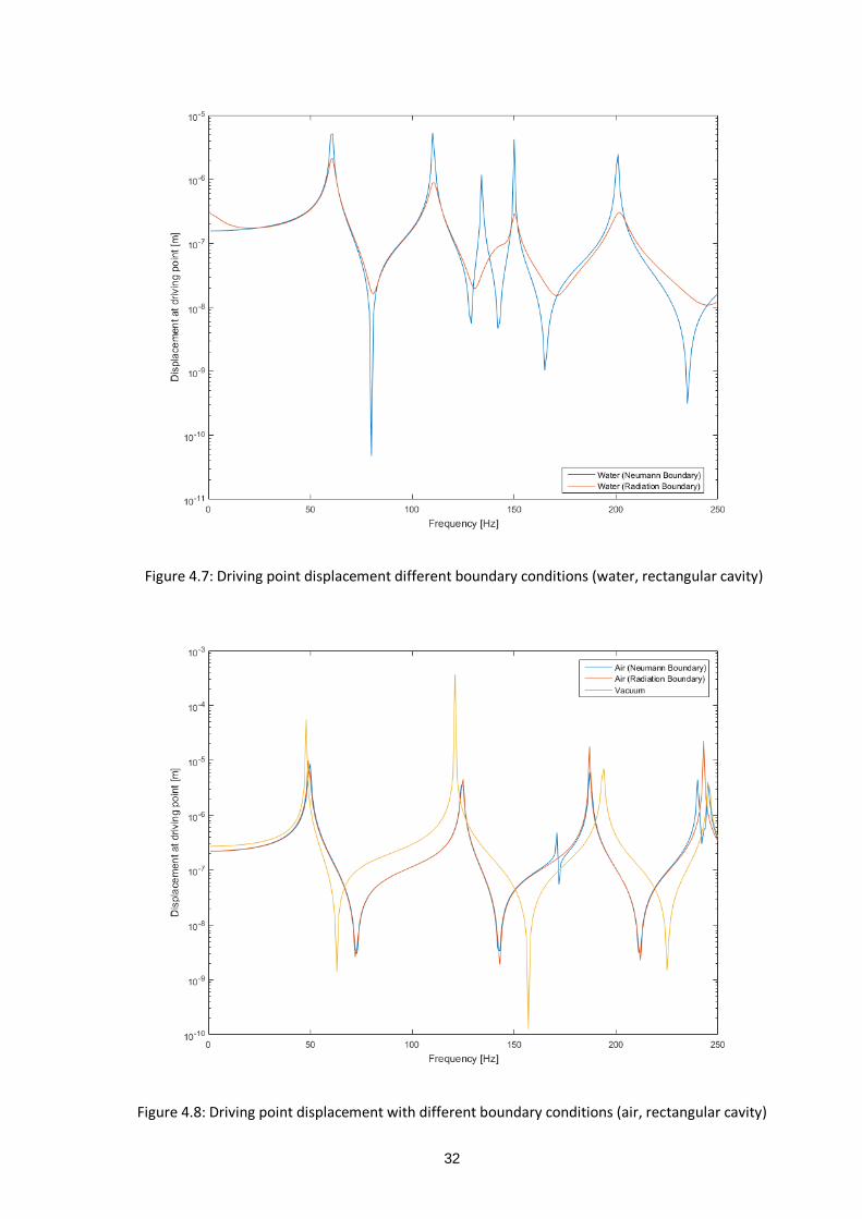
Comparison of boundary conditions
Figure 4.7 shows a comparison of the sound-hard boundary with the radiation boundary. One can see
that the peaks of the curve with the radiation boundary are clearly reduced, as the reflection ratio
compared to the reflecting Neumann curve is much lower. Figure 4.8 then shows the same setting with
the acoustic fluid air and the in vacuo case. It thus can be shown that the influence of the reflection is
not as huge as the acoustic fluid water and the influence of the absorbing boundary is not as high.
Figure 4.6: Comparison of the first four mode shapes
32
Figure 4.7: Driving point displacement different boundary conditions (water, rectangular cavity)
Figure 4.8: Driving point displacement with different boundary conditions (air, rectangular cavity)

33
4.2 Rectangular Panel on Hemisphere
To be able to compare the different absorbing boundary conditions with each other the plate described
in chapter 4.1 is attached to a hemisphere with the radius 𝑟 = 1𝑚. The origin of the hemisphere lies
at the centre of the plate at (0.5, 0.5)𝑚. At the ground of the hemisphere impedance boundary con-
ditions are applied, corresponding to the FSI and the attached open domain. In addition to the dis-
placement at the driving point, the acoustic pressure at the point (0.475, 0.675, 0.575)𝑚 is being rec-
orded.
Figure 4.10 and Figure 4.11 show the displacement of the driving point on the plane for different
boundary conditions and the in vacuo case. Due to the cavity’s different construction the response
varies from the previous example, showing a more ideal behaviour for a plate swinging in an open
domain. The stiffness of the coupled system does not influence the modes as strongly as in the previous
example and so the added mass effect can now be clearly seen.
Figure 4.9: Plate backed on hemisphere cavity

34
Figure 4.10: Driving point displacement with different boundary conditions (air, hemisphere)
Figure 4.11: Driving point displacement with different boundary conditions (water, hemisphere)

35
The differences between the absorbing boundary conditions are negligible for the displacement of the
driving point, but there are small deviations between the graphs of the radiation boundary and the
infinite element boundary at the point in the acoustic cavity in Figure 4.12 and Figure 4.13. Although
the radiation damping effect in air can not be seen at the driving point, there is a clear damping effect
measuring the acoustic pressure at the point in the cavity. Peaks influenced by the reflection of the
Neumann boundary condition are suppresed or reduced when using an absorbing boundary condition.
Figure 4.12: Acoustic pressure of (0.475, 0.675, 0.575) with absorbing boundary conditions (air)
Figure 4.13: Acoustic pressure of (0.475, 0.675, 0.575) with absorbing boundary conditions (water)
36
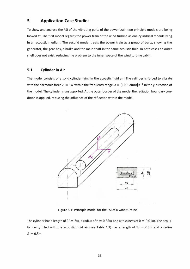
5 Application Case Studies
To show and analyse the FSI of the vibrating parts of the power train two principle models are being
looked at. The first model regards the power train of the wind turbine as one cylindrical module lying
in an acoustic medium. The second model treats the power train as a group of parts, showing the
generator, the gear box, a brake and the main shaft in the same acoustic fluid. In both cases an outer
shell does not exist, reducing the problem to the inner space of the wind turbine cabin.
5.1 Cylinder in Air
The model consists of a solid cylinder lying in the acoustic fluid air. The cylinder is forced to vibrate
with the harmonic force 𝐹 = 1𝑁 within the frequency range Ω = [100: 2000]𝑠−1 in the y-direction of
the model. The cylinder is unsupported. At the outer border of the model the radiation boundary con-
dition is applied, reducing the influence of the reflection within the model.
The cylinder has a length of 2𝑙 = 2𝑚, a radius of 𝑟 = 0.25𝑚 and a thickness of ℎ = 0.01𝑚. The acous-
tic cavity filled with the acoustic fluid air (see Table 4.2) has a length of 2𝐿 = 2.5𝑚 and a radius
𝑅 = 0.5m.
Figure 5.1: Principle model for the FSI of a wind turbine

37
The dominant wave length of the acoustic fluid is
𝜆 =
𝑐
𝑓=
343𝑚𝑠
20001𝑠
= 0.1715𝑚 ( 5.1 )
With the element per wave length condition 𝜆
ℎ𝜆,𝑎𝑖𝑟= 6…8 the recommended element size of the fluid
can be estimated to
ℎ𝜆,𝑎𝑖𝑟 =𝜆
6=
0.1715𝑚
6= 0.0286𝑚 ( 5.2 )
The dominant bending wave length of the cylindrical structure can be determined by
𝜆𝐵 = 2𝜋 ∙ √𝐵
𝑚′
4
∙1
√𝜔= 2𝜋 ∙ √
5.002 ∙ 1016 𝑘𝑔𝑚𝑚3
𝑠2
61.037 ∙ 10−3 𝑘𝑔𝑚𝑚
4
∙1
√2𝜋 ∙ 20001𝑠
= 1686.41𝑚𝑚 ( 5.3 )
𝐵 = 𝐸 ∙ 𝐼 = 2.1 ∙ 105𝑁
𝑚𝑚2∙
𝜋
64(5004 − 4904)𝑚𝑚4 = 5,002 ∙ 1013 𝑁𝑚𝑚2
= 5,002 ∙ 1016𝑘𝑔𝑚𝑚3
𝑠2
𝑚′ = 𝜌 ∙ 𝐴 = 7850𝑘𝑔
𝑚3∙𝜋
4(0.52 − 0.492)𝑚2 = 61.037
𝑘𝑔
𝑚= 61.037 ∙ 10−3
𝑘𝑔
𝑚𝑚
whereby the moment of inertia 𝐼 and the Area 𝐴 are related to an open cylinder. As the recommended
element size of the structure is
ℎ𝜆,𝑠𝑡𝑟𝑢𝑐𝑡𝑢𝑟𝑒 =1.68641𝑚
6= 0.2812𝑚 ( 5.4 )
and the chosen element length is ℎ𝜆,𝑠𝑡𝑟𝑢𝑐𝑡𝑢𝑟𝑒,𝑐ℎ𝑜𝑠𝑒𝑛 = 0.05𝑚 this simplification is not affecting the
results. The model is calculated with the fluid element size ℎ𝜆,𝑎𝑖𝑟 = 0.03𝑚 for frequencies under 𝑓 =
1000 𝐻𝑧 and ℎ𝜆,𝑎𝑖𝑟 = 0.05𝑚 for frequencies above. A constant damping ratio of 𝐷 = 0.002 is applied.
Figure 5.2 shows the frequency response at (0, 0, 0.25)𝑚 of the uncoupled cylinder. The bending
modes of the cylinder are at a frequency of 𝑓 = 514 𝐻𝑧, 𝑓 = 1068𝐻𝑧 and 𝑓 = 1594 𝐻𝑧. The other
peaks correspond to either bending modes of the closed cylinder’s caps, extensional modes or radial
shearing modes. As the bending modes in the normal direction of the applied harmonic force causes
the highest radiation of sound into the acoustic medium they are the only modes being looked at dur-
ing further investigations, showing the influence of mass, stiffness and damping variation on each of
the corresponding modes.

38
Figure 5.2: Displacement of the cylinder at (0, 250, 0) and corresponding mode shapes
Figure 5.3: SPL(A) at (0, 255, 257)
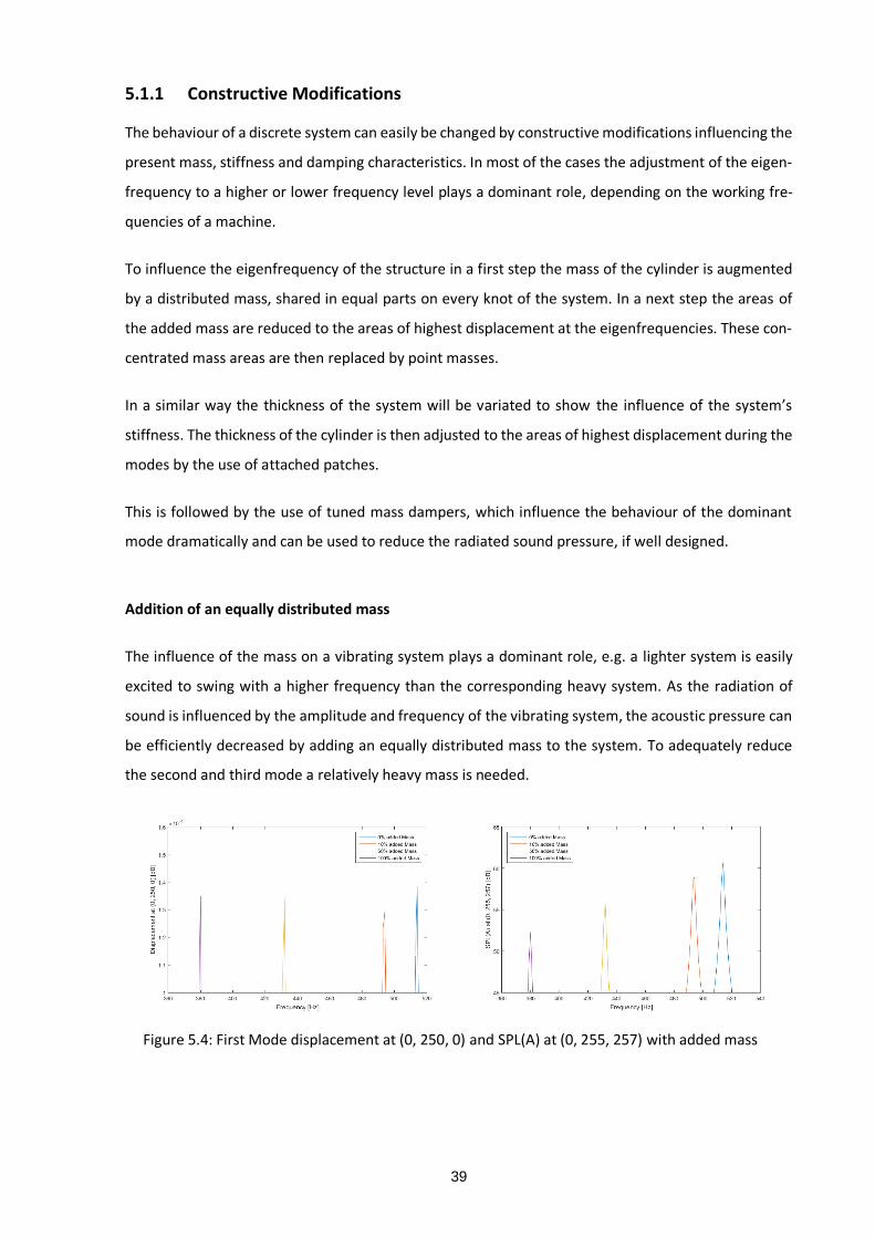
39
5.1.1 Constructive Modifications
The behaviour of a discrete system can easily be changed by constructive modifications influencing the
present mass, stiffness and damping characteristics. In most of the cases the adjustment of the eigen-
frequency to a higher or lower frequency level plays a dominant role, depending on the working fre-
quencies of a machine.
To influence the eigenfrequency of the structure in a first step the mass of the cylinder is augmented
by a distributed mass, shared in equal parts on every knot of the system. In a next step the areas of
the added mass are reduced to the areas of highest displacement at the eigenfrequencies. These con-
centrated mass areas are then replaced by point masses.
In a similar way the thickness of the system will be variated to show the influence of the system’s
stiffness. The thickness of the cylinder is then adjusted to the areas of highest displacement during the
modes by the use of attached patches.
This is followed by the use of tuned mass dampers, which influence the behaviour of the dominant
mode dramatically and can be used to reduce the radiated sound pressure, if well designed.
Addition of an equally distributed mass
The influence of the mass on a vibrating system plays a dominant role, e.g. a lighter system is easily
excited to swing with a higher frequency than the corresponding heavy system. As the radiation of
sound is influenced by the amplitude and frequency of the vibrating system, the acoustic pressure can
be efficiently decreased by adding an equally distributed mass to the system. To adequately reduce
the second and third mode a relatively heavy mass is needed.
Figure 5.4: First Mode displacement at (0, 250, 0) and SPL(A) at (0, 255, 257) with added mass
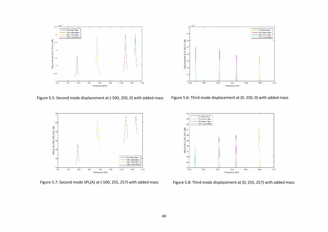
40
Figure 5.5: Second mode displacement at (-500, 250, 0) with added mass Figure 5.6: Third mode displacement at (0, 250, 0) with added mass
Figure 5.7: Second mode SPL(A) at (-500, 255, 257) with added mass Figure 5.8: Third mode displacement at (0, 255, 257) with added mass

41
Distributed mass on selected area
Adding an equally distributed mass on the areas of highest displacement shows nearly the same be-
haviour as adding the same mass onto the whole surface. Figure 5.9, Figure 5.12 and Figure 5.15 show
the areas with the attached weight.
Figure 5.9: First mode and selected area
Figure 5.10: First mode displacement at (0, 250, 0) with area-wide mass
Figure 5.11: First mode SPL(A) at (0, 255, 257) with area-wide mass
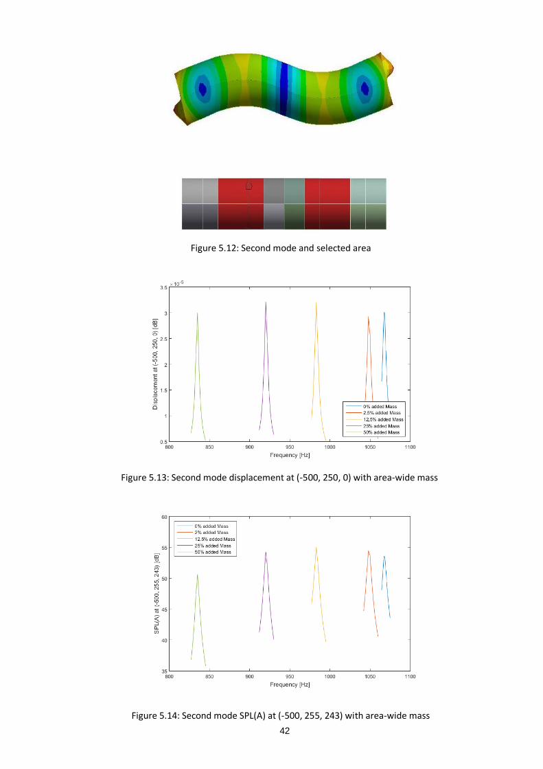
42
Figure 5.12: Second mode and selected area
Figure 5.13: Second mode displacement at (-500, 250, 0) with area-wide mass
Figure 5.14: Second mode SPL(A) at (-500, 255, 243) with area-wide mass

43
Figure 5.15: Third mode and selected area
Figure 5.16: Third mode displacement at (0, 250, 0) and (-500, 250, 0) with area-wide mass
Figure 5.17: Third mode SPL(A) at (0, 255, 257) and (-500, 255, 243) with area-wide mass
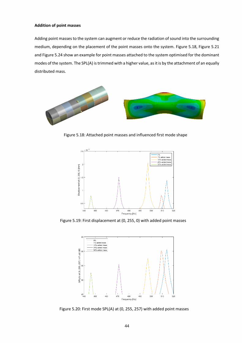
44
Addition of point masses
Adding point masses to the system can augment or reduce the radiation of sound into the surrounding
medium, depending on the placement of the point masses onto the system. Figure 5.18, Figure 5.21
and Figure 5.24 show an example for point masses attached to the system optimised for the dominant
modes of the system. The SPL(A) is trimmed with a higher value, as it is by the attachment of an equally
distributed mass.
Figure 5.18: Attached point masses and influenced first mode shape
Figure 5.19: First displacement at (0, 255, 0) with added point masses
Figure 5.20: First mode SPL(A) at (0, 255, 257) with added point masses

45
Figure 5.21: Attached point masses and influenced second mode shape
Figure 5.22: Second mode displacement at (0, 250, 0) with added point masses
Figure 5.23: Second mode SPL(A) at (-500, 255, 257) with added point masses
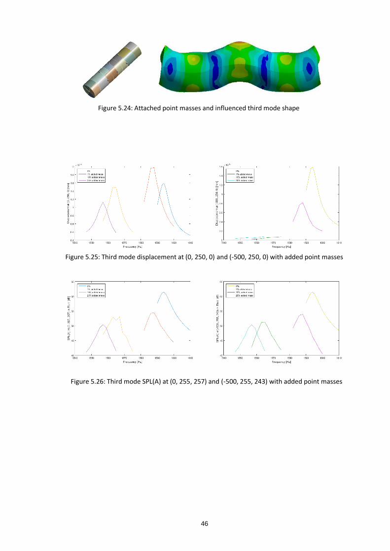
46
Figure 5.24: Attached point masses and influenced third mode shape
Figure 5.25: Third mode displacement at (0, 250, 0) and (-500, 250, 0) with added point masses
Figure 5.26: Third mode SPL(A) at (0, 255, 257) and (-500, 255, 243) with added point masses

47
Variation of the thickness
Varying the thickness of the system’s outer shell results in a higher frequency due to the added stiff-
ness effect. By increasing the weight of the system dramatically the damping effect shows an excellent
reduction of the SPL for the mode shapes with a non-zero average flux over the interface (in this case
the first and the third mode). The second mode first reacts by an added stiffness effect, but then
changes to an added mass effect, reducing the frequency in a forceful way.
Figure 5.27: First mode displacement at (0, 250, 0) with added thickness
Figure 5.28: First mode SPL(A) at (0, 255, 257) with added thickness

48
Figure 5.29: Second mode displacement at (-500, 250, 0) with added thickness Figure 5.30: Third mode displacement at (0, 250, 0) with added thickness
Figure 5.31: Second mode SPL(A) at (-500, 255, 243) with added thickness Figure 5.32: Third mode SPL(A) at (0, 255, 257) with added thickness

49
Addition of patches
To influence the modes directly, patches according to Figure 5.9, Figure 5.11 and Figure 5.15 are at-
tached to the system in the regions of highest displacement. It is a good choice to reduce the sound
pressure without heavily increasing the weight of the system. Figure 5.33 to Figure 5.36 show the dis-
placement and SPL(A) for a patch with the same material as the original system; so it appears more
along the lines of a variation of the outer shell thickness on selected areas. The added patches can be
made from different materials, e.g. sound absorbing bitumen, butyl rubber materials or materials with
higher modal damping values.
The damping of the radiated sound pressure is more efficient if the added masses are huge. In case of
the second mode, the added thickness has to be larger than 𝑡 = 15𝑚𝑚 to show any improvement on
the radiated sound pressure at all. By augmenting the mass on the patches for the side peaks of the
third mode (Figure 5.36, right graph), the radiation of sound pressure could be improved for the cases
with a high middle peak’s patch thickness 𝑡1.
Figure 5.33: First mode displacement at (0, 250, 0) and SPL(A) at (0, 255, 257) with patch
Figure 5.34: Second mode displacement at (-500, 250, 0) and SPL(A) at (-500, 255, 243) with patches

50
Figure 5.35: Third mode displacement at (0, 250, 0) and (-500, 250, 0) with added patches
Figure 5.36: Third mode SPL(A) at (0, 255, 257) and (-500, 255, 243) with added patches
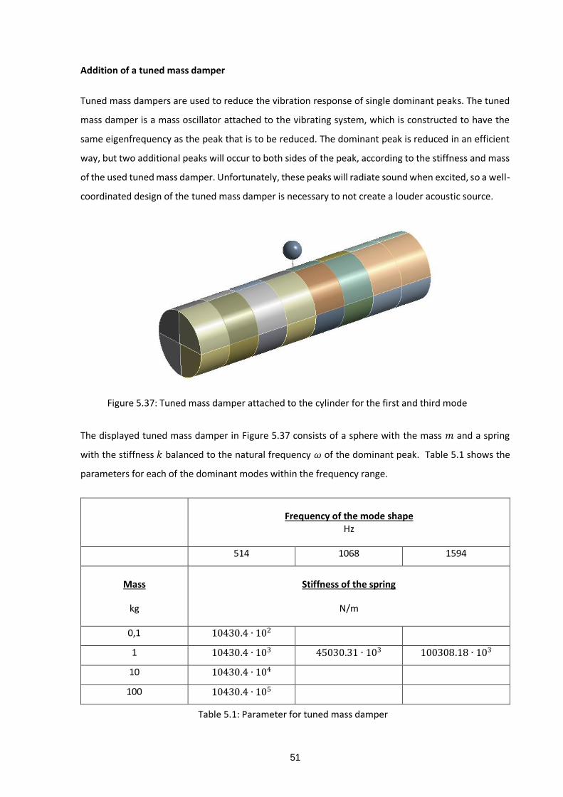
51
Addition of a tuned mass damper
Tuned mass dampers are used to reduce the vibration response of single dominant peaks. The tuned
mass damper is a mass oscillator attached to the vibrating system, which is constructed to have the
same eigenfrequency as the peak that is to be reduced. The dominant peak is reduced in an efficient
way, but two additional peaks will occur to both sides of the peak, according to the stiffness and mass
of the used tuned mass damper. Unfortunately, these peaks will radiate sound when excited, so a well-
coordinated design of the tuned mass damper is necessary to not create a louder acoustic source.
The displayed tuned mass damper in Figure 5.37 consists of a sphere with the mass 𝑚 and a spring
with the stiffness 𝑘 balanced to the natural frequency 𝜔 of the dominant peak. Table 5.1 shows the
parameters for each of the dominant modes within the frequency range.
Frequency of the mode shape
Hz
514 1068 1594
Mass
kg
Stiffness of the spring
N/m
0,1 10430.4 ∙ 102
1 10430.4 ∙ 103 45030.31 ∙ 103 100308.18 ∙ 103
10 10430.4 ∙ 104
100 10430.4 ∙ 105
Figure 5.37: Tuned mass damper attached to the cylinder for the first and third mode
Table 5.1: Parameter for tuned mass damper

52
Figure 5.38 and Figure 5.39 show the first mode displacement and SPL(A) with tuned mass dampers of
different masses. It can be shown that the created peak of dominated stiffness is converging to a fre-
quency, whereas the mass dominated peak is lowering its frequency due to the added mass effect. By
increasing the mass of the tuned mass damper the radiated SPL of the stiffness dominated peak is
rising as well, whereas the SPL of the mass dominated peak is decreasing with the decline of the fre-
quency.
Figure 5.42 shows an example of a badly coordinated tuned mass damper design, as the mass domi-
nated peak’s SPL(A) is higher than the SPL(A) of the original system. Adding a higher mass to the tuned
mass damper could solve this problem, but this will lead to the increase of the second peak; which is
almost on the same level as the dominant peak of the system without a tuned mass damper. Conse-
quently, other constructive modifications should have priority.
Figure 5.38: First mode displacement at (0, 250, 0) with added tuned mass damper
Figure 5.39: First mode SPLA at (0, 255, 257) with added tuned mass damper
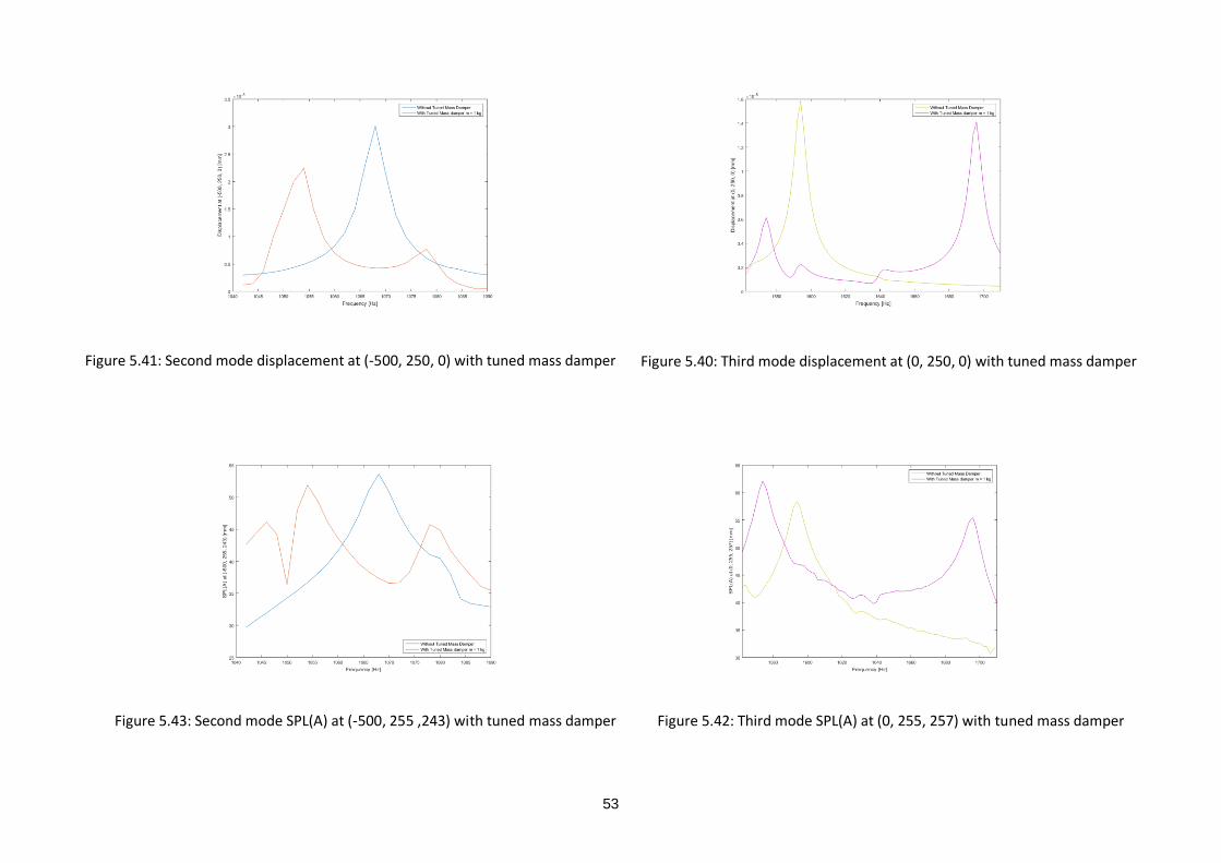
53
Figure 5.40: Third mode displacement at (0, 250, 0) with tuned mass damper Figure 5.41: Second mode displacement at (-500, 250, 0) with tuned mass damper
Figure 5.42: Third mode SPL(A) at (0, 255, 257) with tuned mass damper Figure 5.43: Second mode SPL(A) at (-500, 255 ,243) with tuned mass damper

54
5.2 Power Train in Air
The simplified model shows a power train (consisting of a gear box, a generator, a break, and a part of
the main shaft) lying in the acoustic fluid air. The parts of the power train are forced to vibrate with
the harmonic force 𝐹 = 1𝑁 within the frequency range Ω = [100: 2000]𝑠−1 in the x-direction of the
model. The model is unsupported and a constant damping ratio of 𝐷 = 0.002 is used. At the outer
border of the model the radiation boundary condition is applied.
Figure 5.44: Power train in air
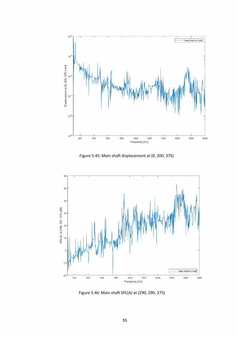
55
Figure 5.45: Main shaft displacement at (0, 200, 375)
Figure 5.46: Main shaft SPL(A) at (290, 290, 375)

56
Figure 5.47: Gear box displacement at (0, 300, 1175)
Figure 5.48: Gear Box SPL(A) at (290, 290, 1175)

57
Figure 5.49: Brake displacement at (-100, 200, 1750)
Figure 5.50: Brake SPL(A) at (290, 290, 1750)

58
Figure 5.51: Generator displacement at (-100, 200, 2100)
Figure 5.52: Generator SPL(A) at (290, 290, 2100)

59
5.2.1 Constructive Modifications
As the SPL augment along with the frequency, constructive modification of the mass is realised for the
frequency of 𝑓 = 1766 𝐻𝑧 as an example. At this frequency the generator of the power train shows
some mode shapes. The modification is applied to the generator only.
Figure 5.53: Displacement figure of the power train at 1766 Hz
Figure 5.54: Generator displacement at (-100, 200, 2100) with added mass

60
Figure 5.55: Generator SPL(A) at (290,290,2100) with added mass

61
6 Conclusion
The vibro-acoustic simulation is a fast and efficient tool to analyse the behaviour of the fluid-structure
coupled system. Changes can be quickly realised and investigated regarding different settings and
solution methods.
The first verification example has indicated an accordance to the analytical solution, while the modified
system has shown the similarity between the different absorbing boundary conditions. The influence
of the boundary reflection could be impaired by the cavity’s different construction; whereby a spheri-
cal hull is the fluid’s optimal body for open domain problems. The use of PML could not be realised
due to the strict setup, but is a possible alternative for further studies.
Detailed investigations were held on the cylindrical principle model, as it showed the influence of the
system’s eigenmodes regarding the radiation of sound into the acoustic domain. The applied construc-
tive modifications resulted in a great improvement on the radiated sound pressure, if the influence of
the added mass and added stiffness to the system was distinct, meaning a great shift in the frequency
of the dominant peak for the added mass or a major damping effect on the displacement amplitude
for the added stiffness. Varying the thickness in the regions of highest displacement at the part’s outer
shell, e.g by the addition of fitted patches, or adding point masses can support the reduction of the
sound pressure without adding too much weight to the system. The use of a well-designed tuned mass
damper can help to reduce the SPL for lower eigenfrequencies, but is counterproductive for higher
modes. The detailed model of the power train confirmed the carried out improvements, as well as the
use of the cylindrical model as a simplification of the power train. The recorded frequency response of
the sound pressure clearly marks the sound emitting frequencies.
In the course of the upcoming research project X-Energy the presented model of the power train can
be improved by creating the support of the power train within the wind turbine cabin. With the crea-
tion of the cabin’s outer shell the influence of the power train’s sound radiation for a point outside the
cavity could be analysed. The implementation of the manufacturer’s model of a power train could help
to reduce the sound radiation in a more specific way, before enhancing and validating the model.

62
7 Literature
[1] A.J. Pretlove: Free Vibrations of a Rectangular Panel Backed by a Closed Rectangular Cavity. In: Journal of Sound and Vibration, S. 197–209
[2] 14.8. Mode-Superposition Method, ANSYS Inc., ANSYS 17.0 Help ANSYS Help System/Mechani-cal APDL/Theory Reference /14. Analysis Tools
[3] 8.3. Propagation, Radiation, and Scattering of Acoustic Pressure Waves, ANSYS Inc., ANSYS 17.0 Help ANSYS Help System/Mechanical APDL/Theory Reference /8.Acoustics
[4] 8.4. Acoustic Fluid-Structural Interaction (FSI), ANSYS Inc., ANSYS 17.0 Help ANSYS Help Sys-tem/Mechanical APDL/Theory Reference /8.Acoustics
[5] ANSYS Mechanical APDL Acoustic Analysis Guide, ANSYS Inc., Theory Reference /Acoustic Analy-sis Guide
[6] AACTx_R170_L_01_Introduction to Acoustics, ANSYS Inc., Bestandteil der ANSYS ACT Acoustics Extension 2014
[7] AACTx_R170_L_03_Harmonic Analyses, ANSYS Inc., Bestandteil der ANSYS ACT Acoustics Exten-sion 2014
[8] Baumann, B., Stein, U. u. Wolff, M.: Physik für Ingenieure. Bachelor Basics ; mit 21 Tabellen. Wil-burgstetten: Schlembach 2011
[9] Beranek, L. L. (Hrsg.): Noise and vibration control engineering. Principles and applications. A Wiley Interscience publication. New York u.a.: Wiley 1992
[10] Franck, A.: Finite-Elemente-Methoden, Lösungsalgorithmen und Werkzeuge für die akustische Simulationstechnik. Techn. Hochsch., Diss.--Aachen, 2008. Aachener Beiträge zur technischen Akustik, Bd. 9. Berlin: Logos-Verl. 2009
[11] Frank Ihlenburg: Computational Methods for Vibroacoustic Simulations. Hamburg 2014
[12] Technische Schwingungslehre, Frank Ihlenburg, 2014
[13] Teilvorhabenbeschreibung Vibroakustik. Vibroakustische Optimierung der Haupttriebstrang-komponenten einer Windenergieanlage (VakuOm), Frank Ihlenburg u. Thomas Grätsch, 2016
[14] Howard, C. Q. u. Cazzolato, B. S.: Acoustic analyses using Matlab and Ansys. Boca Raton, Florida: CRC Press 2015
[15] Leissa, A. W.: Vibration of plates. Woodbury, NY: American Institute of Physics 1993
[16] Lerch, R., Sessler, G. u. Wolf, D.: Technische Akustik. Grundlagen und Anwendungen. Berlin, Hei-delberg: Springer Berlin Heidelberg 2009
[17] M. Fischer u. L. Gaul: Fast BEM–FEM mortar coupling for acoustic–structure interaction. In: In-ternational Journal for Numerical Methods in Engineering, S. 1677–1690
[18] Möser, M.: Technische Akustik. VDI-Buch. Berlin, Heidelberg: Springer Vieweg 2015
[19] Möser, M. u. Kropp, W.: Körperschall. Physikalische Grundlagen und technische Anwendungen. Berlin, Heidelberg: Springer-Verlag Berlin Heidelberg 2010

63
[20] Ryan Bemrose: Louder Sounds Better, Microsoft Developer Blog 2007. https://blogs.msdn.microsoft.com/audiofool/2007/02/07/louder-sounds-better, abgerufen am: 20.08.2016
[21] Wagner, S., Bareiß, R. u. Guidati, G.: Wind Turbine Noise. Berlin, Heidelberg: Springer 1996
[22] Wikibooks.org: Acoustics/Fundamentals of Psychoacoustics, 2012. https://en.wiki-books.org/wiki/Acoustics/Fundamentals_of_Psychoacoustics, abgerufen am: 20.08.2016

A-1
8 Appendix
8.1 Guide to ACT Acoustics in ANSYS Workbench
This guide shows the main functions of the ACT Acoustics Extension and their set-up in the rectangular
plate on cavity example examined in this work. The ACT Acoustics Extension is a free extension, which
can be downloaded in the ANSYS Customer Portal. All the here presented content is implemented in
ANSYS Mechanical APDL. A detailed guideline can be found in the help section of the program.
8.1.1 Installing the Extension
Once downloaded from the customer portal the extension
can be easily installed by using Install Extension under Exten-
sions. After the installation the extension can be found under
Manage Extensions. The extension has to be picked manually
at every new project.
8.1.2 Setting up the FSI Example
Considering the rectangular plate on cavity example the flexible
plate is attached to the left of the rectangular cavity. Both have
structural steel assigned as material. As this cannot be true for the
acoustic fluid an Acoustic Body has to be applied to the cavity, which
overwrites the pre-assigned properties to acoustic relevant proper-
ties.
Figure 8.4: Selecting the Acoustic Body
Figure 8.3: Rectangular Plate on Cavity Example
Figure 8.2: Installing the Extension
Figure 8.1: Inside the Extensions Manager

A-2
The scope of the acoustic domain can be
selected by direct geometric selection or a
prepared named selection. The main
properties of the acoustic fluid can be de-
fined in the Acoustic Body. The most im-
portant of this settings are already pre-de-
fined by the acoustic fluid air. The refer-
ence pressure values are important for
the further researches (e.g. for the evalu-
ation of the SPL) and should better not be
changed, if there is no need for it. Under
Acoustic-Structural Coupled Body Options
the symmetric and unsymmetric matrix formulation can be chosen VERWEIS AUF FLUID-STRUCTURE-
INTERACTION. In case of a FSI problem it is very important to use either Program Controlled Coupled
or Coupled With Symmetric Algorithm for the fluid element layer on the FSI Interface.
As coupled associated elements uses four DOF per knot it is recommended to use another fluid body
with the uncoupled tag right behind it, to minimize the computational times with just one DOF per
element knot (s. chapter 3.3). The coupling between the two domains is therefore implemented at the
first layer of the acoustic domain. As long as not indicated by an additional boundary condition the two
acoustical bodies are regarded as one acoustic domain.
Figure 8.6: Setting of the FSI [14]
Figure 8.5: Details of the Acoustic Body
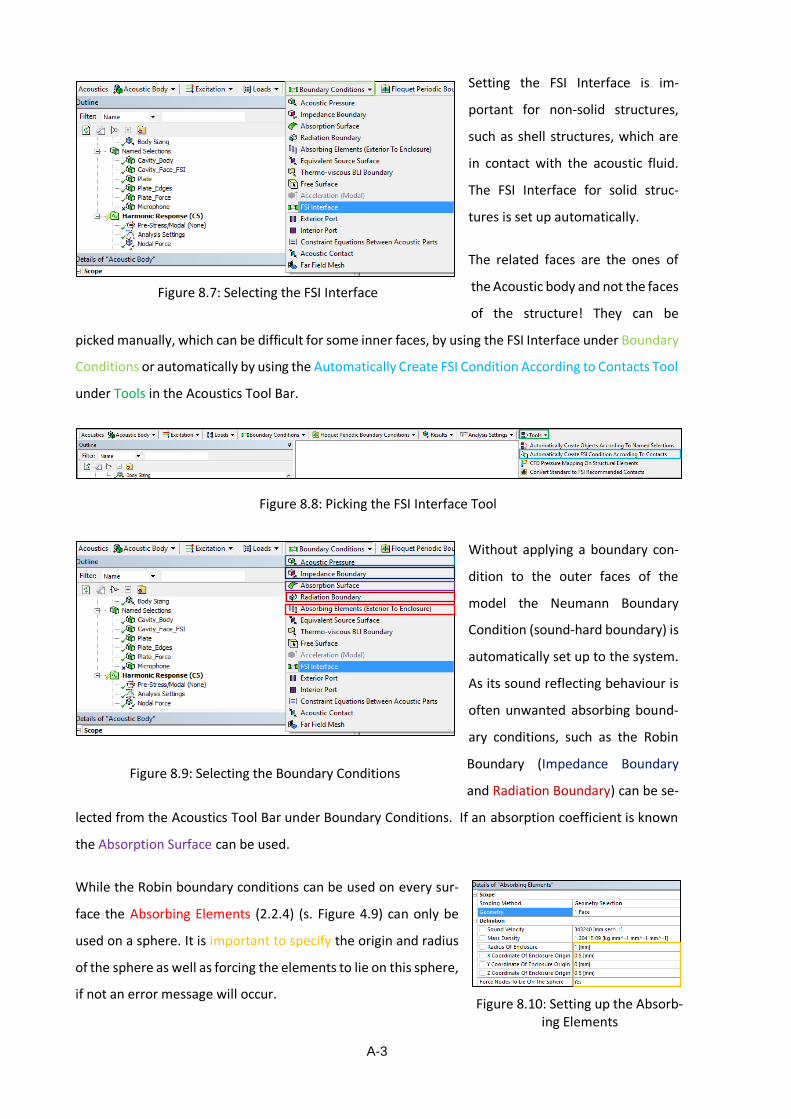
A-3
Setting the FSI Interface is im-
portant for non-solid structures,
such as shell structures, which are
in contact with the acoustic fluid.
The FSI Interface for solid struc-
tures is set up automatically.
The related faces are the ones of
the Acoustic body and not the faces
of the structure! They can be
picked manually, which can be difficult for some inner faces, by using the FSI Interface under Boundary
Conditions or automatically by using the Automatically Create FSI Condition According to Contacts Tool
under Tools in the Acoustics Tool Bar.
Without applying a boundary con-
dition to the outer faces of the
model the Neumann Boundary
Condition (sound-hard boundary) is
automatically set up to the system.
As its sound reflecting behaviour is
often unwanted absorbing bound-
ary conditions, such as the Robin
Boundary (Impedance Boundary
and Radiation Boundary) can be se-
lected from the Acoustics Tool Bar under Boundary Conditions. If an absorption coefficient is known
the Absorption Surface can be used.
While the Robin boundary conditions can be used on every sur-
face the Absorbing Elements (2.2.4) (s. Figure 4.9) can only be
used on a sphere. It is important to specify the origin and radius
of the sphere as well as forcing the elements to lie on this sphere,
if not an error message will occur.
Figure 8.8: Picking the FSI Interface Tool
Figure 8.7: Selecting the FSI Interface
Figure 8.9: Selecting the Boundary Conditions
Figure 8.10: Setting up the Absorb-ing Elements

A-4
In the analysis settings of the harmonic
analysis the solution settings have to be
defined. The requested frequency range
can be inserted by a linear scale, logarith-
mic scale and in octave bands. The solution
interval defines the steps within the fre-
quency span.
The solution method can be chosen be-
tween the direct method and modal super-
position. The use of Variational technol-
ogy, meaning a mixture of both solution
methods, is not recommended.
Some results need the General Miscellane-
ous and the Ansys MAPDL DB to be acti-
vated for their post-processing.
Modal damping can be applied by inserting a constant damping ratio 𝐷 or using Rayleigh Damping by
setting the stiffness 𝛽 and/or mass coefficient 𝛼.
As result the frequency response of
displacement at the driving point
and the acoustic response of a point
in the cavity are of interest.
Therefore, the Frequency Response
of the Deformation is used from the
Solution Toolbar. We are interested
in the deformation in the y-direc-
tion. The y-axis of the chart is loga-
rithmic to clearly show the peaks of
the response.
Figure 8.12: Selecting the frequency response for the deformation of the structure
Figure 8.11: Analysis Settings of a Hamonic Analysis
Figure 8.13: Setting up the frequency response
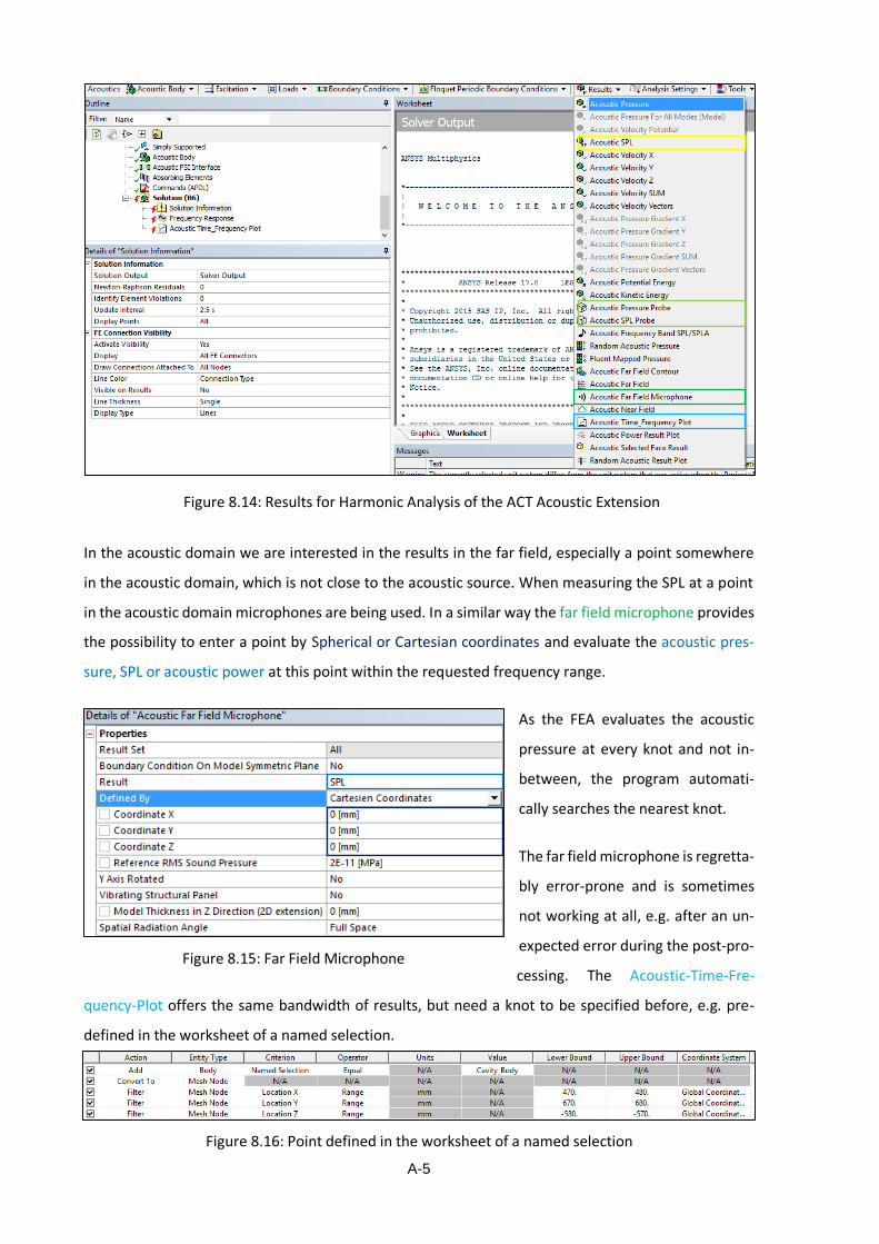
A-5
In the acoustic domain we are interested in the results in the far field, especially a point somewhere
in the acoustic domain, which is not close to the acoustic source. When measuring the SPL at a point
in the acoustic domain microphones are being used. In a similar way the far field microphone provides
the possibility to enter a point by Spherical or Cartesian coordinates and evaluate the acoustic pres-
sure, SPL or acoustic power at this point within the requested frequency range.
As the FEA evaluates the acoustic
pressure at every knot and not in-
between, the program automati-
cally searches the nearest knot.
The far field microphone is regretta-
bly error-prone and is sometimes
not working at all, e.g. after an un-
expected error during the post-pro-
cessing. The Acoustic-Time-Fre-
quency-Plot offers the same bandwidth of results, but need a knot to be specified before, e.g. pre-
defined in the worksheet of a named selection.
Figure 8.14: Results for Harmonic Analysis of the ACT Acoustic Extension
Figure 8.15: Far Field Microphone
Figure 8.16: Point defined in the worksheet of a named selection
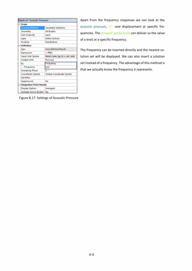
A-6
Apart from the frequency responses we can look at the
acoustic pressure, SPL and displacement at specific fre-
quencies. The acoustic probe tools can deliver us the value
of a knot at a specific frequency.
The frequency can be inserted directly and the nearest so-
lution set will be displayed. We can also insert a solution
set instead of a frequency. The advantage of this method is
that we actually know the frequency it represents.
Figure 8.17: Settings of Acoustic Pressure

A-7
8.1.3 Setting the Mode-Superposition Method
The mode superposition method can be set as the solution method of a FSI problem, if absorbing
boundary conditions are not required and other damping methods, apart from modal damping, are
not considered.
The mode superposition method is set in the analysis set-
tings under solution method. The modal frequency range,
along with the number of modes to find, can remain pro-
gram controlled or set manually. Residual vectors can en-
hance the solution of the mode-superposition, but are not
supported by the unsymmetric eigensolver and therefore
cannot be used during modal-superposition of a system
with FSI coupling in ANSYS.
As only the unsymmetric MAPDL solver
can be used within the mode-superposi-
tion method, the Acoustic-Structural Cou-
pled Body Options has to be changed to
Program Controlled Coupled within the
acoustic body details.
At last the Unsymmetric Harmonic
Mode Superposition has to be se-
lected from the Analysis Settings of
the Acoustics Toolbar in case of the
bi-directional coupling between the
fluid and the structure.
Without this setting or an equivalent
MAPDL command the solver is not set properly and will create an error message while the evaluation
of the mode-superposition.
Figure 8.19: Setting of the Acoustic Body for Mode-Superposition
Figure 8.18: Analysis Settings for Mode-Superposition
Figure 8.20: Unsymmetric Harmonic Mode Superposition

A-8
8.2 ANSYS Mechanical ADPL Scripts
The use of the Ansys Workbench is a quite comfortable way of solving a problem using ANSYS, but in
case of the acoustic analysis it requires an additional extension. Another way to solve an acoustic prob-
lem is the use of mechanical ADPL, often referred as Classic ANSYS. It offers all the possibilities of the
program; of which many are not implemented into the workbench.
The interface is obsolescent and it is quite complicated to build and analyse the model using the avail-
able tools. Therefore, it is more efficient to write a script using the mechanical ADPL language and read
it into the program.
With the use of MAPDL the two main examples are been created parallel to their counterparts in AN-
SYS Workbench. Because of the more user friendly interface regarding changes of the model the Work-
bench gained priority.
8.2.1 MAPDL Rectangular Plate on Rectangular Cavity
FINISH /CLEAR ! Pre-Processing /PREP7 ! Material properties of fluid in cavity speedair = 344 ! Speed of Sound of air [m/s] dens_air = 1.21 ! Density of Air [kg/m^3] ! Material properties of flexible plate platedens = 7900 ! Density [kg/m^3] plate_E = 210e9 ! Youngs modulus [Pa] plate_mu = 0.32 ! Poissons Ratio [-] ! Dimensions of the cavity box_x = 1 ! Length [m] box_y = 1 ! Width [m] box_z = 1 ! Height [m] ! Thickness of the plate. plate_t = 0.01 ! Thickness [m]

A-9
! Defining the Fluid Element (with FSI) ET,1,FLUID30,,1 ! Element type Fluid 30 with 4 DOF MP,SONC,1,speedair ! Material Property Speed of Sound MP,DENS,1,dens_air ! Material Property Density MP,MU,1,0.00 ! Material Property Damping R,1,20e-6 ! Real Constant for Reference pressure ! 20uPa ! Defining the Fluid Element (without FSI) ET,2,FLUID30,,0 ! Element Type Fluid 30 with 1 DOF MP,SONC,2,speedair MP,DENS,2,dens_air MP,MU,2,0.00 R,2,20e-6 ! Defining the Shell Element for the structure R,3,plate_t ! Defining Plate Thickness as Real ! Constant ET,3,SHELL181 ! Element Type Shell 181 SECTYPE,,SHELL SECDATA,plate_t, MP,EX,3,plate_E ! Material Property Young’s Module MP,DENS,3,platedens ! Material Property Density MP,NUXY,3,plate_mu ! Material Property Poisson’s Ratio ! Create the acoustic cavity BLOCK,0,box_x,0,box_y,0,-box_z ! Meshing ESIZE,0.05 ! Set element size TYPE,1 REAL,1 MAT,1 VMESH,ALL ! Volume Meshing NSEL,S,LOC,Z,0 ! Selecting the Face for Plate TYPE,3 REAL,3 MAT,3 ESURF,ALL ESEL,S,TYPE,,3 ! Change all the elements touching the ! plate to FSI NELEM ENODE ESEL,R,TYPE,,1 TYPE,2 REAL,2 MAT,2 EMODIF,ALL SF,ALL,FSI,1

A-10
ESEL,S,TYPE,,2 ! Constrain the Displacement DOF for the ! other fluid elements NELEM NSEL,U,LOC,Z,0 D,ALL,UX D,ALL,UY D,ALL,UZ ! Setting the Simply Supported Boundary at the Edges of the plate ESEL,S,TYPE,,3 NSLE,S,1 NSEL,R,EXT D,ALL,UZ NSEL,S,LOC,Z,0 NSEL,R,LOC,X,0 D,ALL,UX NSEL,S,LOC,Z,0 NSEL,R,LOC,Y,0 D,ALL,UY ALLSEL EPLOT ! Apply force to the plate f_node=NODE(0.20000,0.3000,0.0) F,f_node,FZ,1 ! Solution /SOLU ANTYPE,3 HROPT,FULL ! Direct Solution HROUT,ON LUMPM,0 ! Lumped Matrix Off EQSLV,FRONT,1e-006, ! Specifying the Solver PSTRES,0 HARFRQ,1,250, ! Requested Frequency Range NSUBST,249, ! Number of Substeps KBC,1 ! Load Step is Stepped SAVE SOLVE SAVE ! Post-Processing /POST26 LINES,100000 FILE,'file','rst','.' PRCPLX,1 /gropt,logy,1 ! Retrieve the displacement at the drive point on the plate NSOL,2,f_node,UZ

A-11
! Retrieve the pressure at a point inside the cavity p_node=NODE(0.2,0.3,-0.5) NSOL,3,p_node,PRES ! Plot the drive point displacement /AXLAB,X,Frequency [Hz] /AXLAB,Y,Displacement [m] PLVAR,2 ! Export the drive point displacement /OUTPUT,d_node,txt PRVAR,2 /OUTPUT ! Export the pressure inside the cavity /OUTPUT,p_node,txt PRVAR,3 /OUTPUT
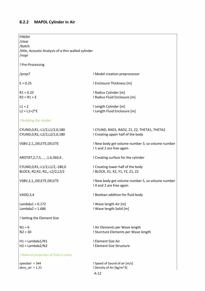
A-12
8.2.2 MAPDL Cylinder in Air
FINISH /clear /batch /title, Acoustic Analysis of a thin walled zylinder /nopr ! Pre-Processing /prep7 ! Model creation preprocessor E = 0.25 ! Enclosure Thickness [m] R1 = 0.25 ! Radius Cylinder [m] R2 = R1 + E ! Radius Fluid Enclosure [m] L1 = 2 ! Length Cylinder [m] L2 = L1+2*E ! Length Fluid Enclosure [m] ! Building the model CYLIND,0,R1,-L1/2,L1/2,0,180 ! CYLIND, RAD1, RAD2, Z1, Z2, THETA1, THETA2 CYLIND,0,R2,-L2/2,L2/2,0,180 ! Creating upper half of the body VSBV,2,1,,DELETE,DELETE ! New body get volume number 3, so volume number ! 1 and 2 are free again AROTAT,2,7,5, , , ,1,6,360,4 , ! Creating surface for the cylinder CYLIND,0,R1,-L1/2,L1/2,-180,0 ! Creating lower half of the body BLOCK,-R2,R2,-R2,,-L2/2,L2/2 ! BLOCK, X1, X2, Y1, Y2, Z1, Z2 VSBV,2,1,,DELETE,DELETE ! New body get volume number 5, so volume number ! 4 and 2 are free again VADD,3,4 ! Boolean addition for fluid body Lambda1 = 0.172 ! Wave length Air [m] Lambda2 = 1.686 ! Wave length Solid [m] ! Setting the Element Size N1 = 6 ! Air Elements per Wave length N2 = 30 ! Sturcture Elements per Wave length H1 = Lambda1/N1 ! Element Size Air H2 = Lambda2/N2 ! Element Size Structure ! Material properties of fluid in cavity speedair = 344 ! Speed of Sound of air [m/s] dens_air = 1.21 ! Density of Air [kg/m^3]
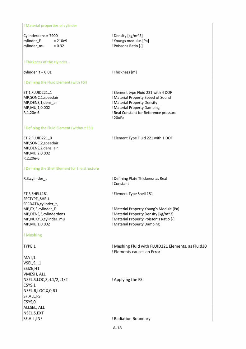
A-13
! Material properties of cylinder Cylinderdens = 7900 ! Density [kg/m^3] cylinder_E = 210e9 ! Youngs modulus [Pa] cylinder_mu = 0.32 ! Poissons Ratio [-]
! Thickness of the clyinder. cylinder_t = 0.01 ! Thickness [m] ! Defining the Fluid Element (with FSI) ET,1,FLUID221,,1 ! Element type Fluid 221 with 4 DOF MP,SONC,1,speedair ! Material Property Speed of Sound MP,DENS,1,dens_air ! Material Property Density MP,MU,1,0.002 ! Material Property Damping R,1,20e-6 ! Real Constant for Reference pressure ! 20uPa ! Defining the Fluid Element (without FSI) ET,2,FLUID221,,0 ! Element Type Fluid 221 with 1 DOF MP,SONC,2,speedair MP,DENS,2,dens_air MP,MU,2,0.002 R,2,20e-6 ! Defining the Shell Element for the structure R,3,cylinder_t ! Defining Plate Thickness as Real ! Constant ET,3,SHELL181 ! Element Type Shell 181 SECTYPE,,SHELL SECDATA,cylinder_t, MP,EX,3,cylinder_E ! Material Property Young’s Module [Pa] MP,DENS,3,cylinderdens ! Material Property Density [kg/m^3] MP,NUXY,3,cylinder_mu ! Material Property Poisson’s Ratio [-] MP,MU,1,0.002 ! Material Property Damping
! Meshing TYPE,1 ! Meshing Fluid with FLUID221 Elements, as Fluid30 ! Elements causes an Error MAT,1 VSEL,S,,,1 ESIZE,H1 VMESH, ALL NSEL,S,LOC,Z,-L1/2,L1/2 ! Applying the FSI CSYS,1 NSEL,R,LOC,X,0,R1 SF,ALL,FSI CSYS,0 ALLSEL, ALL NSEL,S,EXT SF,ALL,INF ! Radiation Boundary

A-14
ALLSEL, ALL TYPE,3 ! Meshing Solid MAT,3 FLST,5,12,5,ORDE,12 ! List the areas to mesh FITEM,5,4 FITEM,5,5 FITEM,5,9 FITEM,5,10 FITEM,5,13 FITEM,5,14 FITEM,5,15 FITEM,5,16 FITEM,5,17 FITEM,5,18 FITEM,5,19 FITEM,5,20 ASEL,S,,,P51X ! Selecting the listet areas ESIZE,H2 AMESH,ALL ALLSEL,ALL f_node=NODE(R1,0,L1/2) F,f_node,FX,1
FINISH ! Solution /SOLU ANTYPE,3 HROPT,FULL ! Direct Solution HROUT,ON LUMPM,0 ! Lumped Matrix Off EQSLV,FRONT,1e-006, ! Specifying the Solver PSTRES,0 HARFRQ,100,2000, ! Requested Frequency Range NSUBST,9, ! Number of Substeps KBC,1 ! Load Step is Stepped SAVE SOLVE SAVE ! Post-Processing /POST26 LINES,100000 FILE,'file','rst','.' PRCPLX,1 /gropt,logy,1 ! Retrieve the displacement at the drive point on the plate NSOL,2,f_node,UX
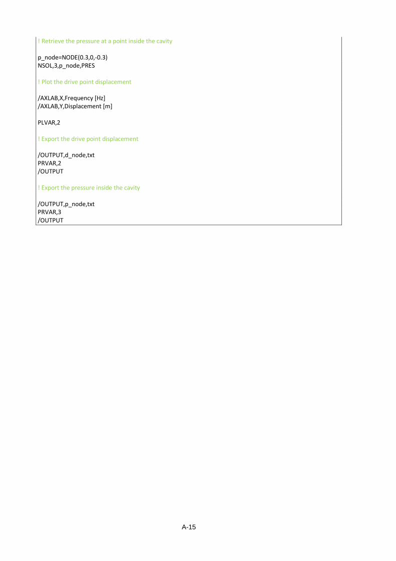
A-15
! Retrieve the pressure at a point inside the cavity p_node=NODE(0.3,0,-0.3) NSOL,3,p_node,PRES ! Plot the drive point displacement /AXLAB,X,Frequency [Hz] /AXLAB,Y,Displacement [m] PLVAR,2 ! Export the drive point displacement /OUTPUT,d_node,txt PRVAR,2 /OUTPUT ! Export the pressure inside the cavity /OUTPUT,p_node,txt PRVAR,3 /OUTPUT

A-16
8.3 Matlab Rectangular Plate on Rectangular Cavity (after Howard [14])
clc clear all % Dimensions of the cavity cavity.len_x = 1; % [m] cavity.len_y = 1; % [m] cavity.len_z = 1; % [m] cavity.volume = cavity.len_x .* cavity.len_y .* cavity.len_z; % [m^3] % Parameters of the fluid fluid.density = 1000; % [kg/m^3] density of the gas fluid.speed = 1481; % [m/s] speed of sound of the gas % Dimensions of the plate plate.len_x = cavity.len_x; % [m] plate.len_y = cavity.len_y; % [m] plate.thick = 0.01; % [m] surfacearea = plate.len_x .* plate.len_y; % Material properties of Steel plate.density = 7900; % [kg/m^3] density plate.E = 2.1e11; % [Pa] Youngs modulus plate.mu = 0.3; % [no units] Poissons Ratio % Define location of acoustic source speaker.loc_x=0.1; speaker.loc_y=0.1; speaker.loc_z=0.1; speaker.vol_velocity=0; % Define the location of the microphone mic.loc_x=0.2; mic.loc_y=0.3; mic.loc_z=0.5; % Define the point load on the plate force.loc_x = 0.2; force.loc_y = 0.3; force.amp = 1; % amplitude of the force

A-17
% Define location of accelerometer accel.loc_x = force.loc_x; accel.loc_y = force.loc_y;
% Define the number of structural and acoustic modes to use nstrmodes = 100; % number of structural modes to use ncavmodes = 200; % number of acoustic modes to use % Define the analysis frequency range freq_vect = [1:250]; % [Hz] end_freq = freq_vect(length(freq_vect)); % Calculate the resonance frequencies of the cavity n_max = 50; fprintf('===Start calculation of the resonance frequencies of the cavity\n'); mode_index=[]; for ii=0:n_max for jj = 0:n_max for kk = 0:n_max mode_index = [ mode_index ; ii jj kk ]; end; end; end; % Calculate the resonance frequencies of the cavity res_freq = sqrt( (mode_index(:,1) / cavity.len_x).^2 + ... (mode_index(:,2) / cavity.len_y).^2 + ... (mode_index(:,3) / cavity.len_z).^2 ); res_freq = res_freq .* fluid.speed ./ 2; % [Hz] % sort the resonance frequencies temp=sortrows([res_freq mode_index],1); res_freq = temp(:,1); mode_index = temp(:,2:4); % Use only first 1:ncavmodes cavity.res_freq = res_freq(1:ncavmodes); cavity.mode_index = mode_index(1:ncavmodes,:);

A-18
% Calculate the modal volume epsilon_modal_volume = zeros(size(cavity.mode_index)); index2change = find(cavity.mode_index(:,1)==0); epsilon_modal_volume(index2change,1) = 1; index2change = find(cavity.mode_index(:,1)>0); epsilon_modal_volume(index2change,1) = 0.5; index2change = find(cavity.mode_index(:,2)==0); epsilon_modal_volume(index2change,2) = 1; index2change = find(cavity.mode_index(:,2)>0); epsilon_modal_volume(index2change,2) = 0.5; index2change = find(cavity.mode_index(:,3)==0); epsilon_modal_volume(index2change,3) = 1; index2change = find(cavity.mode_index(:,3)>0); epsilon_modal_volume(index2change,3) = 0.5; cavity.modalvolume = cavity.volume ... .* epsilon_modal_volume(:,1) ... .* epsilon_modal_volume(:,2) ... .* epsilon_modal_volume(:,3); % Evaluate the mode shapes at the microphone locations cavity.phi_eval = ... cos(cavity.mode_index(:,1)*pi*mic.loc_x.'/cavity.len_x) .* ... cos(cavity.mode_index(:,2)*pi*mic.loc_y.'/cavity.len_y) .* ... cos(cavity.mode_index(:,3)*pi*mic.loc_z.'/cavity.len_z); % Evaluate the mode shapes at the acoustic source location speaker.phi_eval = ... cos(cavity.mode_index(:,1)*pi*speaker.loc_x.'/cavity.len_x) .* ... cos(cavity.mode_index(:,2)*pi*speaker.loc_y.'/cavity.len_y) .* ... cos(cavity.mode_index(:,3)*pi*speaker.loc_z.'/cavity.len_z); fprintf('===End of calculation of the resonance frequencies of the cavity \n'); % Calculate the resonance frequencies of the plate n_max = 50; fprintf('===Start calculation of the resonance frequencies of the plate\n'); str_mode_index=[]; for ii=1:n_max for jj = 1:n_max str_mode_index = [ str_mode_index ; ii jj ]; end; end;
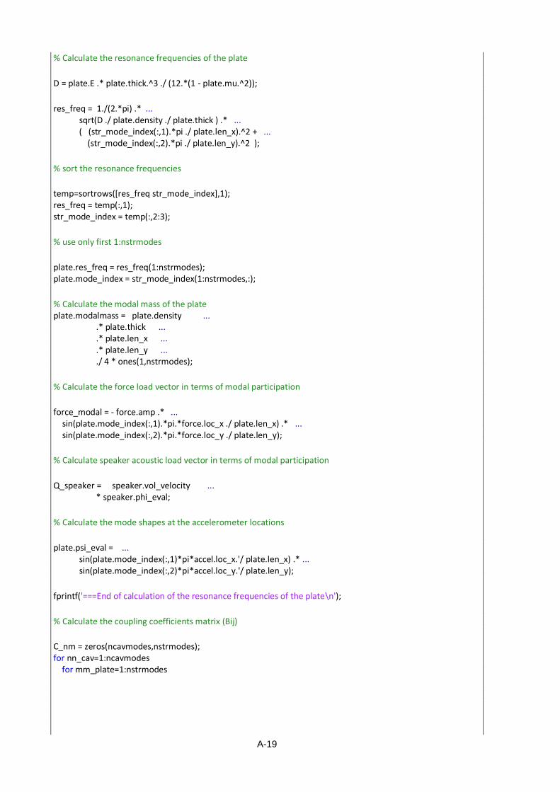
A-19
% Calculate the resonance frequencies of the plate D = plate.E .* plate.thick.^3 ./ (12.*(1 - plate.mu.^2)); res_freq = 1./(2.*pi) .* ... sqrt(D ./ plate.density ./ plate.thick ) .* ... ( (str_mode_index(:,1).*pi ./ plate.len_x).^2 + ... (str_mode_index(:,2).*pi ./ plate.len_y).^2 ); % sort the resonance frequencies temp=sortrows([res_freq str_mode_index],1); res_freq = temp(:,1); str_mode_index = temp(:,2:3); % use only first 1:nstrmodes plate.res_freq = res_freq(1:nstrmodes); plate.mode_index = str_mode_index(1:nstrmodes,:); % Calculate the modal mass of the plate plate.modalmass = plate.density ... .* plate.thick ... .* plate.len_x ... .* plate.len_y ... ./ 4 * ones(1,nstrmodes); % Calculate the force load vector in terms of modal participation force_modal = - force.amp .* ... sin(plate.mode_index(:,1).*pi.*force.loc_x ./ plate.len_x) .* ... sin(plate.mode_index(:,2).*pi.*force.loc_y ./ plate.len_y); % Calculate speaker acoustic load vector in terms of modal participation Q_speaker = speaker.vol_velocity ... * speaker.phi_eval; % Calculate the mode shapes at the accelerometer locations plate.psi_eval = ... sin(plate.mode_index(:,1)*pi*accel.loc_x.'/ plate.len_x) .* ... sin(plate.mode_index(:,2)*pi*accel.loc_y.'/ plate.len_y); fprintf('===End of calculation of the resonance frequencies of the plate\n'); % Calculate the coupling coefficients matrix (Bij) C_nm = zeros(ncavmodes,nstrmodes); for nn_cav=1:ncavmodes for mm_plate=1:nstrmodes
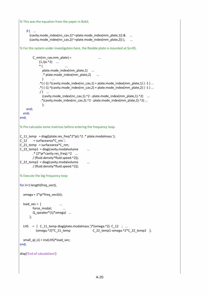
A-20
% This was the equation from the paper in Bokil, if ( ... (cavity.mode_index(nn_cav,1)~=plate.mode_index(mm_plate,1)) & ... (cavity.mode_index(nn_cav,2)~=plate.mode_index(mm_plate,2)) ), ... % For the system under investigation here, the flexible plate is mounted at $z=0$. C_nm(nn_cav,mm_plate) = ... (1./pi.^2) ... * ( ... plate.mode_index(mm_plate,1) ... .* plate.mode_index(mm_plate,2) ... ) ... .*( (-1).^(cavity.mode_index(nn_cav,1) + plate.mode_index(mm_plate,1) ) -1 ) ... .*( (-1).^(cavity.mode_index(nn_cav,2) + plate.mode_index(mm_plate,2) ) -1 ) ... ./ ( ... (cavity.mode_index(nn_cav,1).^2 - plate.mode_index(mm_plate,1).^2) ... .*(cavity.mode_index(nn_cav,2).^2 - plate.mode_index(mm_plate,2).^2) ... ); end; end; end;
% Pre-calculate some matrices before entering the frequency loop. C_11_temp = diag((plate.res_freq*2*pi).^2 .* plate.modalmass.'); C_12 = surfacearea*C_nm.'; C_21_temp = surfacearea*C_nm; C_22_temp1 = diag(cavity.modalvolume ... .* (2*pi*cavity.res_freq).^2 ... / (fluid.density*fluid.speed.^2)); C_22_temp2 = diag(cavity.modalvolume ... / (fluid.density*fluid.speed.^2)); % Execute the big frequency loop
for ii=1:length(freq_vect), omega = 2*pi*freq_vect(ii); load_vec = [ ... force_modal; ... Q_speaker*(1j*omega) ... ]; LHS = [ C_11_temp-diag(plate.modalmass.')*(omega.^2) C_12 ; ... (omega.^2)*C_21_temp C_22_temp1-omega.^2*C_22_temp2 ]; small_q(:,ii) = inv(LHS)*load_vec; end; disp('End of calculations')

A-21
% Separate the modal participation factors struct_q = small_q(1:nstrmodes,:); acoust_q = small_q(nstrmodes+1:nstrmodes+ncavmodes,:); % Calculate some acoustic and structural results sq_struct_q=struct_q.^2; sq_acoust_q=acoust_q.^2; sum_sq_struct_q=sum(sq_struct_q); sum_sq_acoust_q=sum(sq_acoust_q); matlab_ape=1/(4*fluid.density*fluid.speed^2)*cavity.modalvolume.'*abs(acoust_q.^2); matlab_pressure = cavity.phi_eval.' * acoust_q; matlab_sq_p= matlab_pressure.^2; matlab_displacement = plate.psi_eval.' * struct_q; % Plot the acoustic presure at the microphone figure set(gca,'fontsize',16); p1h=semilogy(freq_vect,abs(matlab_pressure)); set(p1h,'linewidth',2); xlabel('Frequency [Hz]'); ylabel('Pressure [Pa]'); title('Acoustic Pressure at a Point in the Cavity'); grid % Plot the displacement at the accelerometer figure set(gca,'fontsize',16); p2h=semilogy(freq_vect,abs(matlab_displacement)); set(p2h,'linewidth',2); xlabel('Frequency [Hz]'); ylabel('Displacement [m]'); title('Plate Displacement at Drive Point'); grid


