Embed Size (px)
Citation preview

THE PREDICTION OF CORPORATE FAILURE USING PRICE ADJUSTED
ACCOUNTING DATA
BY
ISAAC MWANG KIRAGU
A MANAGEMENT PROJECT SUBMITTED IN PARTIAL FULFILMENT OF THE
REQUIREMENT OF THE DEGREE OF MASTER OF BUSINESS AND
ADMINISTRATION, FACULTY OF COMMERCE, UNIVERSITY OF NAIROBI.
JULY, 1991

DECLARATION
This Management Research Project is my original work and has not
been presented for a degree in any other university
Signed ^~rr~ VT ...... Date . / / . . X /........
Ki ragu I . M . •
This
t i on
Management Research
with my approval as
Signed V j v ' j (
Project has been submitted for
university supervisor.
Date
J.M. Karanja
Lecturer (Department of Accounting)
exami na-

DEDICATION
To my fami 1y
Dad: John Kiragu Gichohi
Mum: Loise Wanjiku Kiragu
Brothers: K a r i u k i ,M w a i , N d i r i t u ,K a r u e r u ,N d u n g ’u , Waweru
and Muruthi
Sisters: Gathoni and Wangeci
For their continued encouragement throughout all the years I
was i n school.
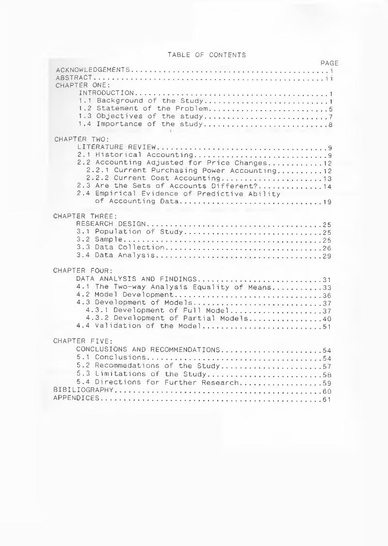
TABLE OF CONTENTSPAGE
ACKNOWLEDGEMENTS.................................................. iABSTRACT...........................................................i iCHAPTER ONE:
INTRODUCTION..................................................11.1 Background of the Study................................ 11.2 Statement of the Problem.............................. 51.3 Objectives of the study................................71.4 Importance of the study................................8
CHAPTER TWO:LITERATURE REVIEW............................................92.1 Historical Accounting.................................. 92.2 Accounting Adjusted for Price Changes............... 12
2.2.1 Current Purchasing Power Accounting........... 122.2.2 Current Cost Accounting.......................... 13
2.3 Are the Sets of Accounts Different?................ 142.4 Empirical Evidence of Predictive Ability
of Accounting Data.....................................19
CHAPTER THREE:RESEARCH DESIGN............................................. 253.1 Population of Study................................... 253.2 Sample................................................... 253.3 Data Collection........................................ 263.4 Data Analysis...........................................29
CHAPTER FOUR:DATA ANALYSIS AND FINDINGS.................... 314.1 The Two-way Analysis Equality of Means.............. 334.2 Model Development......................................364.3 Development of Models................................. 37
4.3.1 Development of Full Model....................... 374.3.2 Development of Partial Models.................. 40
4.4 Validation of the Model.............................. 51
CHAPTER FIVE:CONCLUSIONS AND RECOMMENDATIONS..........................545.1 Conclusions............ 545.2 Recommedations of the Study..........................575.3 Limitations of the Study............................. 585.4 Directions for Further Research..................... 59
BIBILIOGRAPHY..................................................... 60APPENDICES...................................................... .6^

ACKNOWLEDEMENTS
The completion of this Research paper would have been
impossible without invaluable input by the following:
My supervisor Mr. Karanja for his untiring efforts in
guiding me throughout the research period.
Dr. Muragu and Mr Fernandes for their tremendous encourage
ment and moral support when things seemed impossible.
All the Lecturers of the Faculty of Commerce, University of
Nairobi for their effort in making me what I am.
All classmates who encouraged me through the M.B.A
program and finally to brethren whose prayers and
encouragement I will never forget. To all I say a "Big
Thank You."
While recognising the contribution of the above, errors
contained in this project whether of omission or
commission remain my responsibility.

ABSTRACT
This study sought to build a model to predict corporate
failure using accounting data adjusted for price level changes.
The need to predict failure before its actual happening need not
be emphasised given that its a "costly" outcome. The General
price level index was used to adjust the historical accounting
data.
The sample consisted of 10 failed and 10 non-failed com
panies. The seemingly small sample was a consequence of lack of
data availability particulary on the failed companies. This is
surely one of the severe limitations of the study. Important
financial ratios were calculated from price-level adjusted finan
cial statements. The discriminant model developed from this data
showed that nine ratios had a high corporate failure predictive
ability. These ratio’s in order of importance were Times interest
coverage, Fixed Charge coverage, Quick ratio, Current ratio,
Equity to total assets, Working capital to total debt, Retained
earning to total assets, Change in monetary liabilities, Total
debt to total assets and Inventory turnover.
However the most critical ratios were the liquidity and debt
service ratios.
i i

CHAPTER 1
INTRODUCTION
1 . 1 BACKGROUND OF THE STUDY,
One of the well known functions of managers is decision
making. Decision making involves choosing a course of action from
several alternatives. Finance involves three major decision
areas, raising funds, allocating these funds to profitable areas
and the distribution of resultant earnings to owners. The first
decision is known as financing, the second investment and the
third dividend decision.
All decisions affect the future. Knowledge about the future
is thus of critical importance if sound decisions are to be made.
This knowledge is gained through a search for information which
includes accounting information. This information is provided by
accountants in form of financial statements namely the balance
sheet, the income statement and the statement of sources and ap
plication of funds among others. Information contained in the
financial statement is of interest not only to the share holders
but also to other stakeholders such as managers, tax authorities,
the Government, creditors, scholars and potential investors.
This is in line with the contemporary view of the nature of the
firm (the contractual theory) which views a firm as a network of
1
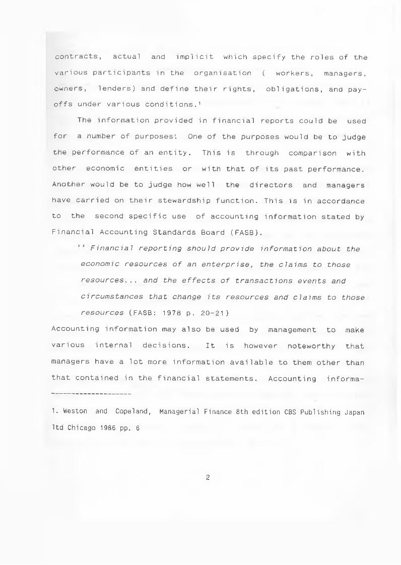
contracts, actual and implicit which specify the roles of the
various participants in the organisation ( workers, managers,
owners, lenders) and define their rights, obligations, and pay
offs under various conditions.1
The information provided in financial reports could be used
for a number of purposes'. One of the purposes would be to judge
the performance of an entity. This is through comparison with
other economic entities or with that of its past performance.
Another would be to judge how well the directors and managers
have carried on their stewardship function. This is in accordance
to the second specific use of accounting information stated by
Financial Accounting Standards Board (FASB).
Financial reporting should provide information about the
economic resources of an enterprise, the claims to those
resources... and the effects of transactions events and
circumstances that change its resources and claims to those
resources (FASB: 1978 p. 20-21)
Accounting information may also be used by management to make
various internal decisions. It is however noteworthy that
managers have a lot more information available to them other than
that contained in the financial statements. Accounting informa-
1. Weston and Copeland, Managerial Finance 8th edition CBS Publishing Japan
ltd Chicago 1986 pp. 6
2
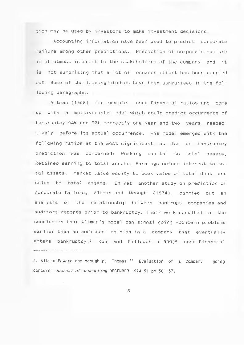
tion may be used by investors to make investment decisions.
Accounting information have been used to predict corporate
failure among other predictions. Prediction of corporate failure
is of utmost interest to the stakeholders of the company and it
is not surprising that a lot of research effort has been carried
out. Some of the leading'studies have been summarised in the fol
lowing paragraphs.
Altman (1968) for example used Financial ratios and came
up with a multivariate model which could predict occurrence of
bankruptcy 94% and 72% correctly one year and two years respec
tively before its actual occurrence. His model emerged with the
following ratios as the most significant as far as bankruptcy
prediction was concerned: Working capital to total assets,
Retained earning to total assets, Earnings before interest to to
tal assets, Market value equity to book value of total debt and
sales to total assets. In yet another study on prediction of
corporate failure, Altman and Mcough (1974), carried out an
analysis of the relationship between bankrupt companies and
auditors reports prior to bankruptcy. Their work resulted in the
conclusion that Altman’s model can signal going -concern problems
earlier than an auditors’ opinion in a company that eventually
enters bankruptcy.2 Koh and Killouch ( 1 9 90)3 used Financial
2. Altman Edward and Mcough p. Thomas ’’ Evaluation of a Company going
concern" Journal of accounting DECEMBER 1974 51 pp 50- 57.
3
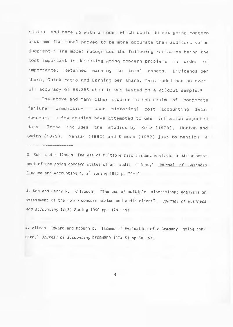
ratios and came up with a model which could detect going concern
problems.The model proved to be more accurate than auditors value
judgment.4 The model recognised the following ratios as being the
most important in detecting going concern problems in order of
importance: Retained earning to total assets, Dividends per
share, Quick ratio and Earn'ing per share. This model had an over
all accuracy of 88.25% when it was tested on a holdout sample.5
The above and many other studies in the realm of corporate
failure prediction used historical cost accounting data.
However, a few studies have attempted to use inflation adjusted
data. These includes the studies by Ketz (1978), Norton and
Smith (1979), Mensah (1983) and Kimura (1982) just to mention a
3. Koh and killouch "The use of multiple Discriminant Analysis in the assess
ment of the going concern status of an audit client," Journal of Business
Finance and Accounting 17(2) spring 1990 pp179-191
4. Koh and Carry N. Killouch, "The use of multiple discriminant analysis on
assessment of the going concern status and audit client". Journal of Business
and accounting 17(2) Spring 1990 pp. 179- 191
5. Altman Edward and Hcough p. Thomas ’’ Evaluation of a Company going con
cern." Journal of accounting DECEMBER 1974 51 pp 50- 57.
4
few.
The conclusions reached thus far, are far from being finite,
and the number of researches into this important area are on the
i ncrease.
1.2 STATEMENT OF THE PROBLEM
One often stated advantage of a company over other types of
business organisations ( i.e Sole proprietorship and partnership)
is that, its assumed to have a perpetual life. In reality
however companies do fail and the assumption of infinite life
collapses. This leads to huge losses not only to the share
holders but also to the other stakeholders. The share holders as
well as other stakeholders therefore are concerned and will look
keenly to any sign of probable failure. If failure could be
detected early it would be possible to minimise failure as
sociated costs. For example the shareholders could withdraw their
investment, the consumers could look for alternative markets; the
manager would make turn-around strategies before it is too late,
while suppliers could look for alternative markets. Managers may
also arrange for the sale of the corporation or even arrange for
a take-over. To be able to predict failure each stakeholder
seeks information from various sources, the most important being
the annual financial statements.
Financial statements can be based on either historical
cost accounting systems (conventional accounting) or price-level
5
adjusted (inflation) accounting data. In the later case changes
in value of money are taken into account.
In an environment of changing value of money it is doubtful
whether historical cost accounting information provide adequate
information to interested parties. This doubt increases espe
cially in developing countries which suffer from hyper
inflation.
A number of studies aimed at comparing the predictive
ability of the two sets of data have been carried out. These
studies have reported mixed results. Studies carried out by Ketz
(1978), Norton and Smith (1987), Mensah (1983) and Keaey and Wat
son (1986) concluded that inflation accounting was not superior
to historical cost accounting. Beaver (1982), Schaefer (1984) and
Ohlsen(1985) used security market prices and concluded the same.
In contrast, Kimura (1982), Bublitz (1985) found significant ad
ditional explanation power of price-level adjusted accounting
data. The conclusions arrived at so far therefore fail to show a
clear preference of one accounting framework ( i.e Historical or
price-level) over the other.
The basic problem of this study is one of coming up with a
model to predict corporate failure using price adjusted account
ing data for kenyan companies. The rate of inflation in kenya has
ranged between 10% and 25% over the last ten years ( i.e the
official rate ), although independent bodies ( eg. united
nations, world-bank, I.M.F and a number of private consulting
6
firms6 ) think its much higher than that stated by the monetary
authorities.
1.3 OBJECTIVES OF THE STUDY
This study is intended to achieve the following objectives,
1. To develop a model using price adjusted accounting
data that can be used to predict corporate failure.
2. To identify critical financial ratios with high
corporate failure predictive abilities under inflationary
conditions.
1.4 IMPORTANCE OF THE STUDY
This study is likely to be of interest to the following,
1. To accounting policy makers who may be interested to know
the ability of inflation accounting data to predict corporate
failure in the Kenyan environment.
2. Financial analysts who will be able to provide more
6. See Nation News paper of may 23rd 1991
7

useful advise to their clients.
3.
research
Scholars who may use this study as a base for further
in the local environment.
8
CHAPTER 2
LITERATURE REVIEW
The basic objective of financial accounting is the prepara
tion of financial statements in a way that gives a true and fair
view of the operating results and the financial position of a
business. Only when financial statements present a true and fair
view of the operating and financial position of the company can
they be of use to decision makers including the prediction of
corporate failure.
Two sets of accounting methods exists presently.
1. Historical accounting (conventional accounting).
2. Price adjusted accounting (inflation accounting).
2.1 HISTORICAL ACCOUNTING
This is the conventional method of accounting and has been
in use for a long time. It records transactions at their
historical cost and provides no adjustments for price changes.
Historical Cost Accounting has been strongly advocated for the
reasons explained in the following few paragraphs;
Historical cost valuation is the only valuation method that
includes as an integral part of its valuation procedure
structure on the double-entry book-keeping system. This is an
9
essential requirements of equity accounting that every actual
change in the resource of the entity be recorded.
Historical cost accounting provides data that are less¥
disputable than that provided under other valuation methods
currently proposed which is a requirement in equity accounting.
It has also been argued that in refusing to recognize
holding gains and loses historical accounting is in line of
maintaining the status quo which is essential in solving
conflict of prices and maintaining order and stability in
society.
It provides data for decision making by insightful managers
and investors so far as history is basis for predicting the
future.7
It is also defended on the basis of cost. It is argued that
it is the least costly for society considering the social cost
of recording, auditing and that of settling disputes.
The historical cost accounting enables the performance of
the custodian function very well. It is good to note that this
is the most fundamental purpose of accounting ( stewardship
role). It is therefore argued that since millions of investors
are relying upon the custodian function of accounting when they
invest in a firm historical accounting system remains useful.
7. Note: History may, however, have little or no relationship with the future
10

This is so because it offers very little room if any, for
manipulation and the information so prepared is objective and can
be relied upon.
Critics of historical accounting point out several
weakness.
They contend it does not provide relevant information, it
overstates profit leading to over-taxation, and it fails to
properly match revenues with their relevant costs, hence
distorting the accounting information. These weaknesses were
noticed as early as 1920. For example Patron in consideration to
this problem concluded that,
"...it is perhaps not unreasonable to argue that the accountant should prepare supplementary statements at the end of the period to show , by making proper allowance for the change in the value of money the true comparative status of the enterprise...." )8
In fact, considering the above argument, other types of
accounting systems offer good supplements rather than
substitutes to historical cost accounting as they are more
subject to manipulation and personal judgment.
8. Littleton and Zimmerman(1920) pp 177.
2.2 ACCOUNTING ADJUSTED FOR PRICE CHANGES
There are two methods of accounting for price changes:
(a) The current purchasing power method or general purchasing
power method (CPP).
(b) Current cost accounting method (CCA).
2.2.1 CURRENT PURCHASING POWER
The CPP method uses conversion factors to transform
accounts prepared under historical cost basis to price
adjusted accounts. Again distinction is made between monetary
items and non-monetary items. Under this method only
non-monetary items need to be transformed since monetary items
are already in current prices at the end of the period. The CPP
suffers from the following weakness:
1. It is based on index numbers which are statistical
averages. It cannot therefore be applied with precision to
individual firms.
2. The selection of the index number is a problem.
Different indices have different characteristics. Hoh Katherine
(1977) found out that gross method procedure deflator
approximates specific price indices in the case of firms with
diversified assets while consumer price index was the •
appropriate index for other.
12
3. The CPP method deals with general price level and not
with changes in individual items except in cases where
individual prices happen to move in step with general price
index.
2.2.2 CURRENT COST ACCOUNTING
This method requires each item in the financial statement
to be restated in the current value. Unlike CPP method no
cognizance is taken of general purchasing cost of money. Asset
items in the balance sheet are shown at prices in which they
would cost at the balance sheet date:
This method has also been found to suffer from the following
weaknesses
1. Though CCA takes care of current year’s depreciation it
fails to provide adequately for backlog depreciation.
2. Also although CCA provides funds for replacing of exist
ing assets it fails to provide for replacement of new type of
assets.
3. It ignores gains or losses on monetary items that arise
as a result of holding monetary assets and liabilities during a
period of changing price levels.
4. CCA is based on the presumption that firms use uniform
accounting methods and practice and therefore fails to recognize
valuation in accounting method
5. CCA has too much subjectivity. For example it does not
1 3

mand any single method of valuation be used. Replacement
lue, market price, and net realizable value all qualify to be
e current cost of an asset under this method.9
Edward and Bell (1962) advocated for the use of
placement cost accounting as the primary method of account-
g. Chamber (1966) demonstrated and advocated the use of exit
ice or the current cost equivalent while Sterling (1970)
vocated for the use of exit price model based on realizable
1 u e .
Recognition that the problem of choosing the right model
J1d not be solved on apriori grounds only lead to much effort
ng put in empirical research.
ARE THE SETS OF ACCOUNT DIFFERENT (HC VS. GPLA)?
IRICAL STUDIES
The main aim of this section is to investigate whether the
sets of accounts are the same or different.
Empirical studies in this area were directed to finding out
ther adjusting historical accounting data for inflation
akes a difference ". They also addressed the question of the
here is a third method which is at its evolutionary state which advocates
use of both the CPP and CCA. Its too early to say how it will operate in
tice.
14
demand any single method of valuation be used. Replacement
value, market price, and net realizable value all qualify to be
the current cost of an asset under this method.9
Edward and Bell (1962) advocated for the use of
replacement cost accounting as the primary method of account
ing, Chamber (1966) demonstrated and advocated the use of exit
price or the current cost equivalent while Sterling (1970)
advocated for the use of exit price model based on realizable
value.
Recognition that the problem of choosing the right model
could not be solved on apriori grounds only lead to much effort
being put in empirical research.
2.3 ARE THE SETS OF ACCOUNT DIFFERENT (HC VS. GPLA)?
EMPIRICAL STUDIES
The main aim of this section is to investigate whether the
two sets of accounts are the same or different.
Empirical studies in this area were directed to finding out
whether adjusting historical accounting data for inflation
makes a difference “ . They also addressed the question of the
9. There is a third method which is at its evolutionary state which advocates
the use of both the CPP and CCA. Its too early to say how it will operate in
practice.
14
significance of the differences .
The following are some of the notable studies:-
Jones (1949) investigated nine steel companies for the
period between 1941 -1947. When adjustments were made on the
actual historical records to determine the restated values in the
financial statements, it was found that in real terms the
companies might have been paying dividend out of capital and that
recorded decrease in fixed assets were much less than was
actually the case when inflation was taken into account. A
replication of this study by Jones (1955) came up with similar
results . This gives empirical evidence that adjustment for price
changes may make a difference in dividend decisions. It is impor
tant to remember that this is one of the most important decisions
that managers are required to make from time to time.
Dyckman (1969) used simulated financial data for two
companies in a field study to assess the magnitude of the
difference in investment decision. He divided his subjects into
three groups and gave them historical cost(HC), general price
level adjusted (GPLA) data and a combination of HC and GPLA
respectively. When subjects were asked to estimate the price
range of the security’s stock using the information provided, the
three types of information resulted in different estimates.
Dyckman concluded that the statements appeared to make a
d i fference.
Dyckman’s findings supports the idea that the sets of
accounting may make a difference in an investment decision.
However a laboratory experiment by Heintz (1973) came with
contradicting results to those of Dyckman’s. Heintz supplied HC,
GPLA and both data of three companies to subjects who were
required to make estimates of company’s end year security prices.
In addition the subjects'were required to make an hypothetical
investment decision in the companies. He found no evidence to
support superiority performance of either HC or GPLA data. He
found the different sets of data made no difference.
Petersen (1973), reported a study of its kind. He used a
computer program developed for the purpose, to adjust financial
statements of 65 companies whose information were publicly
available for general price level changes. He then calculated the
average financial ratios, net income, return on equity and their
respective standard deviations. He found that there was
significant difference between return on equity, its standard
deviation and the standard deviations of income of the two sets
of data (HC and GPLA). This study supported the idea that general
price adjustments tend to result in a displacement in financial
parameters. Petersen however was unable to determine whether the
displacement was significant from a decision making point of view
or not.
Mckenzie (1975) conducted a similar inquiry to that of
Petersen for the airline industry. He calculated seven ratios
which he used to rank the nine firms in his sample. He found that
1 6
the two sets of data did not lead to significant difference in
the ranking. Deninies (1976) tested magnitudes of the difference
between HC and GPLA based ratios. He found significant dif
ference between nineteen ratios out of the twenty he had
selected. This has been supported by recent studies.
For example Baran, Lakonishok and Ofer (1980) concluded that :
"The result obtained appear to support the hypothesis that the price level adjusted data contain information which is not included in the financial report currently provided"10 This may be a reason why the two sets of accounts should be
considered as complementary rather than substitutes as they may
contain completely different information.
Davidson and Weil (1974) studied the effect of FASB’S
exposure draft on price-level adjustments.11
By comparing the result with those obtained with HC he
reported that the effect of adjusting for purchasing power on
10. Baran, Aron, J. , Lakonishok and A. R. Ofer. " The information Content of
General Price Level Adjusted Earnings: Some Empirical Evindence," The Ac
counting Review, January (1980) pp.34
11. Note The above refers to the " Financial reporting in units of general
purchasing power" proposed statement by the financial accounting standard
board 1974 .
various financial measures eg. profitability , liquidity and
return on capital were mixed and were likely to depend on the
capital and financial structure of the firm. Studies by Davidson
and Weil (1975) and Stickney (1976) included many types of firms
(24 utilities, 12 steel companies, 12 pharmaceuticals, 6 motor
vehicles and 44 other industries) reported that although GPLA net
income after recognizing gain or loss or net monetary items was
surprisingly high in relation to conventionally reported net in
come, in general the rate of return calculated from GPLA amount
were less than those calculated from statements whether the
measure was return on equity or return on total assets.
From the studies so far reviewed, a number of conclusions
can be made.
1. The results produced by the two sets of accounts may be
different as evidenced by the studies .
2. The price adjusted accounting data may contain addi
tional information, if not different information from that con
tained in historical cost accounts.
3. The effect of adjustment for the price level changes on
accounts may be affected by the internal and external environment
of a firm. Managers decide the financial and capital structure of
the firm which affects the result of price level adjustment.
4. It might be difficult to decide which set of accounting
is better suited for what situation, for example, making future
dec i s i ons.
1 8
5. To get maximum benefit of accounting information it may
be necessary to use both sets of accounting systems
2.5 EMPIRICAL EVIDENCE OF CORPORATE FAILURE PREDICTIVE ABILITY OF
ACCOUNTING DATA.
Numerous studies investigating the ability to predict Busi
ness failure have been carried out in the last three decades.
One of the first scholars to be interested with the predict
ive ability of accounting data was Beaver (1966) who conducted a
number of studies. Beaver set a study to find out whether
accounting ratios could be used to predict failure. Using a
univariate model he found that certain accounting ratios could
very well discriminate between failed and non-failed firms.
He identified the following ratios as better discriminators:
(a) Cash flow to total debts12
(b) Net income to total assets
(c) Total debt to total assets
(d) Working capital to total assets and
(e) Current assets to current debt .
Five years before failure according to Beaver, the above
ratios of failed firms differed significantly from those of
non-failed firms. In 1968 Beaver set a study to find out whether
12. Note This was the best ratio

liquid ratios were superior to non liquid ratios in discriminat
ing between failed and non-failed firms. He found out that
non-liquid ratios were more accurate in discriminating between
failed and non-failed firms than were the liquid ratios. From
the above two studies one message is very clear. Accounting
information can be used td discriminate between failed and non-
failed fi rms.
A study that has remained a landmark in this area is that
done by Altman in 1968. Altman, using a mathematical method
(multivariate discriminant analysis) came up with a discriminant
function which could predict bankruptcy 95% and 72% cor
rectly one year and two years before the occurrence of bankruptcy
respectively (correct here is referring to the ability of the
model to correctly classify firms into their apriori groups).
In this model the following ratios emerged as the most
i mportant:
(a) Working capital to total assets
(b) Retained earnings to total assets
(c) Earning before interest and taxes to total assets
(d) Market value of equity to book value of debt and
(e) Sales to total assets.
Another study concerned with predictive ability of account
ing data is that of Norton (1976). He had a sample of 60 com
panies (30 bankrupt and 30 non-bankrupt). After adjusting for
20
price level changes using a computer program developed by Peter
sen (1971) ratios were computed from both sets of data.
Although the predictive ability of the two models did not
differ significantly (being 81%-90% for the best HC model and
8 1 8 8 % for the best GPLA model ), Norton observed that GPLA
ratios did show higher 'levels of significance in terms of
univariate discriminant ability when partial F-ratios were ob
served.Thus it can be concluded that GPLA data is not inferiorto
HC data.
Altman (1977) used a new data base adjusted to take into ac
count the latest financial accounting standards used Multivariate
Discriminant Analysis with both linear and quadratic structures.
He came up with a model which he named the Newer Zeta Model
which was far more accurate than his 1968 model. This new Zeta
model had the following ratios in it: Return on total assets,
stability of earnings (measured by the normalised measure of
standard error of estimate around some ten year trend in return
on assets ), debt service ratio (earnings before interest and
taxes to total interest payment), retained earnings to total as
sets , current assets to current liabilities, equity to total
capital and size measured by the firm’s total assets.13
13. Since the new model improved due to taking adjustments required by the
latest financial standards one may conclude that financial standards improve
predictive ability of accounting data.
21
Dambolena and Khoury (1980) collected data for 68 firms (34
failed and 34 non failed ). They came up with a ratio based
model which classified firms 91.3% , 84.8*, 82.6* , 89.1* and
78* accuracy one year, two years, three years, four years and
five years respectively prior to failure. The high accuracy was
achieved as a result of incorporating stability variables into
the model. This may indicate that accounting information posses
corporate failure predictive power if appropriate (other unknown)
variables still available in the accounting statements are incor
porated in the models.
Kimura (1982) used a sample of 45 firms ( 21 bankrupt and 24
non-bankrupt firms). He adjusted the financial statements for
general price level using a Fortran program developed by Peter
sen (1971). By using stepwise discriminant analysis he developed
a linear discriminant function for both historical as well as
GPLA data. He concluded thus:
“A cursory examination of the accuracy achieved indicates that GPLA data are marginally more accurate, that is, they are either more accurate or at least as accurate as HC ratios”.14 This finding once again may lead to the conclusion that GPLA ac
counting data may contain additional information not otherwise
available in historical accounting data.
14. op sit pp.66
22
The following ratios were found to be most significant in
predicting bankruptcy in Kimura’s ( 1982) study :-
1. Monetary assets to monetary liabilities,
2. Total liabilities to total assets,
3. Net income to Average owners equity,
4. Earning before in'terest and taxes to total assets,
5. Change in the net book value of fixed assets and
6. Net sales to Total assets.
In a recent study Koh and Killough (1987) used stepwise
discriminant analysis and came up with a historical cost model
for predicting corporate failure. The model had an overall ac
curacy of 92.65%. The following ratios emerged as the most impor
tant .
1. Quick ratio
2. Retained earnings to Total assets
3. Earnings per share
4. Dividend per share.
Though accounting information (specifically accounting
ratios) may be inappropriate predictors in some situations15 the
15. Accounting ratios are poor discriminators between non-failed firms and
failed firms that are only financially distressed for a while.
23
above studies provide evidence that accounting data provide
useful information for prediction of failure. To date, it is
difficult to establish which set of accounts are better in pre
dicting corporate failure. However there is much evidence to sup
port the thesis that GPLA is not inferior to historical cost ac
counting. To get maximum' benefits from accounting information and
recognising that the two sets of accounts are most likely com
plimentary rather than substitutes it may be recommended that
both sets of accounts be used simultaneously.
24
CHAPTER 3
RESEARCH DESIGN
3.1 POPULATION OF STUDY
The population of 'interest consists of those limited
liability companies that were in the register of Registrar of
Companies any time between 1980 and 1990. The population was
split into two groups. The first group consisted of those com
panies that failed during the 1980 - 1990 period while the second
group those that did not fail.16
3.2 THE SAMPLE
The original intention was to select a sample of 30 com
panies from each group. However only ten failed companies had a
complete set of financial statements available from any im
aginable source. The sources explored and from which financial
statements were sought included the registrar of companies offi
cial receiver, the Nairobi stock exchange and the offices of the
leading public accounting firms which are also involved in
receivership work.
16. Failed companies referred here are those that went into receivership
during the period of interest.
25
This meant that no sampling of failed companies could be un
dertaken and hence a census for all the 10 firms was done. Each
failed firm was then matched with a similar firm whose financial
statements were available and which did not fail during the
period. The matching was based on size measured in terms of the
value of total assets.17'
3.3 DATA COLLECTION
Annual accounts for four years prior to failure were col
lected for the failed companies. The same was done for the non-
failed companies included in the sample. The financial statements
for two years prior to failure were then adjusted for price
level changes using the Gross Domestic Product Deflator. The GDP
deflator index numbers were provided by the central bureau of
statistic. The GDP deflator index numbers were used for the
simple reason that they were readily available. While the GDP
deflator may not be correct it nevertheless approximates the cor
rect index.
17. Equal numbers for the two groups were used because this would improve the
reliability of the results(Lehmann, 1985)
26
The following financial ratios were calculated from the
price-level adjusted financial statements ( See appendex C):
1. Current Ratio
2. Quick ratio
3. Working Capital to Total Debt
4. Equity to Total 1 Liabi1ities
5. Total Debt to Total Assets
6. Times interest earned
7. Fixed Charge coverage
8. Retained earnings to Total assets
9 Profit margin on sales
10. Return on Total assets
11. Return on Net worth
12. Inventory Turnover
13. Average Collection Period
14. Fixed asset turnover
15. Sales to Total Assetsy
16. Monetary Asset to Monetary liabilities
17. Monetary liabilities to Total assets
18. Monetary asset to Total assets
19. Change in monetary Liabilities (Year t to Year t+1)
The above ratios were selected on the basis of being common
ratios or having been used elsewhere in business failure pre
diction related studies.
27

Some of the studies in which
significant are listed bellow.
RATIO
Current ratio
Working Capital to Total'debt
Equity to Total Liabilities
Retained earning to Total assets
Return on Total assets
Return on net worth
Fixed asset turnover
Sales to Total assets
Monetary assets to Monetary
liabilities.
Monetary liabilities to
Total assets.
Monetary assets to
Total assets.
Change in monetary
liabilities.
Quick Ratio, Times interest
the Profit margin on sales were
the above ratios were found to be
STUDY
Beaver (1966) , Altman (1977)
Altman (1968)
Altman (1977), Beaver (1966),and
Kimura(1982)
Altman (1977)
Beaver ( 1966 ) ,A 1tman( 1968)
Kimura ( 1982 )
Kimura (1982)
Kimura (1982)
Kimura (1982), Altman (1968)
Kimura (1982)
and
the sample as
known to students of finance.
earned, Fixed charge turnover
also included in
they are common ratios and are well
28
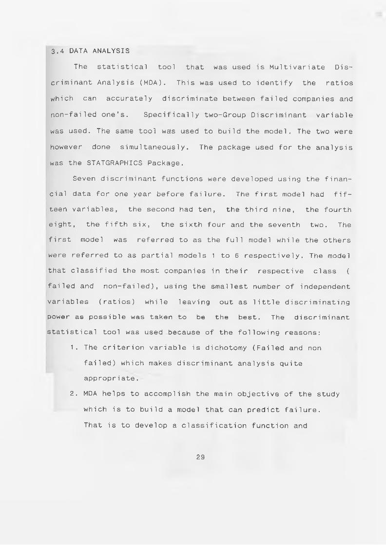
3.4 DATA ANALYSIS
The statistical tool that was used is Multivariate Dis
criminant Analysis (MDA). This was used to identify the ratios
which can accurately discriminate between failed companies and
non-failed o n e ’s. Specifically two-Group Discriminant variable
was used. The same tool was used to build the model. The two were
however done simultaneously. The package used for the analysis
was the STATGRAPHICS Package.
Seven discriminant functions were developed using the finan
cial data for one year before failure. The first model had fif
teen variables, the second had ten, the third nine, the fourth
eight, the fifth six, the sixth four and the seventh two. The
first model was referred to as the full model while the others
were referred to as partial models 1 to 6 respectively. The model
that classified the most companies in their respective class (
failed and non-failed), using the smallest number of independent
variables (ratios) while leaving out as little discriminating
power as possible was taken to be the best. The discriminant
statistical tool was used because of the following reasons:
1. The criterion variable is dichotomy (Failed and non
failed) which makes discriminant analysis quite
appropri ate.
2. MDA helps to accomplish the main objective of the study
which is to build a model that can predict failure.
That is to develop a classification function and
29

a cut-off point for
failed firms). This
the two groups (failed and non
is possible because
the mathematical objective of discriminant analysis is to weight and linearly combine the discriminating variables in some fashion so that the groups are forced to be as statistically distinct as possible".
( Klecka, 1975:435).
30
CHAPTER 4
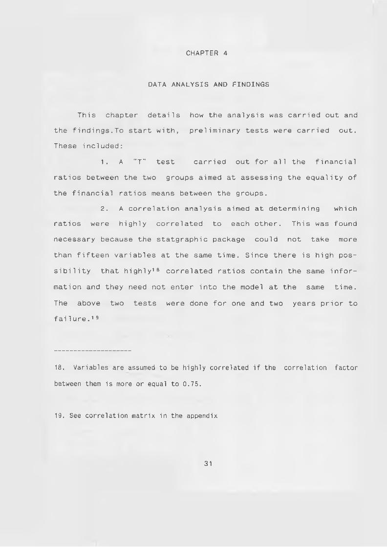
DATA ANALYSIS AND FINDINGS
This chapter details how the analysis was carried out and
the findings.To start with, preliminary tests were carried out.
These included:
1. A "T" test carried out for all the financial
ratios between the two groups aimed at assessing the equality of
the financial ratios means between the groups.
2. A correlation analysis aimed at determining which
ratios were highly correlated to each other. This was found
necessary because the statgraphic package could not take more
than fifteen variables at the same time. Since there is high pos
sibility that highly18 correlated ratios contain the same infor
mation and they need not enter into the model at the same time.
The above two tests were done for one and two years prior to
failure.19
18. Variables are assumed to be highly correlated if the correlation factor
between them is more or equal to 0.75.
19. See correlation matrix in the appendix
31
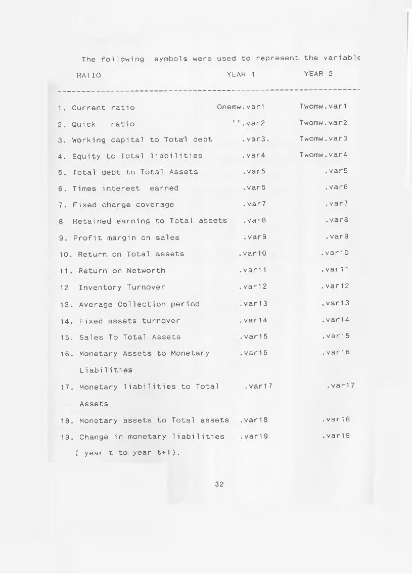
The following symbols were used to represent the variable
RATIO YEAR 1 YEAR 2
1. Current ratio Onemw . var 1 Twomw.var1
2. Quick ratio . var2 Twomw.var2
3. Working capital to Tota'l debt .var3. Twomw.var3
4. Equity to Total liabilities . var4 Twomw.var4
5 . Total debt to Total Assets . var5 . var5
6 . Times interest earned . var6 . var6
7 . Fixed charge coverage . var7 . var7
8 Retained earning to Total assets . var8 . var8
9. Profit margin on sales . var9 .var9
10 . Return on Total assets var 1 0 . var10
1 1 . Return on Networth var 11 .var11
12 Inventory Turnover var 1 2 . var12
13 . Average Collection period var 1 3 . var13
14 . Fixed assets turnover var 14 . var14
15 . Sales To Total Assets var 1 5 . var15
16 . Monetary Assets to Monetary var 1 6 . var16
Liabi1ities
17 . Monetary liabilities to Total . var17 . var 1
Assets
18 . Monetary assets to Total assets var 1 8 . var18
1 9 . Change in monetary liabilities var 1 9 . var19
( year t to year t+1 ).
32
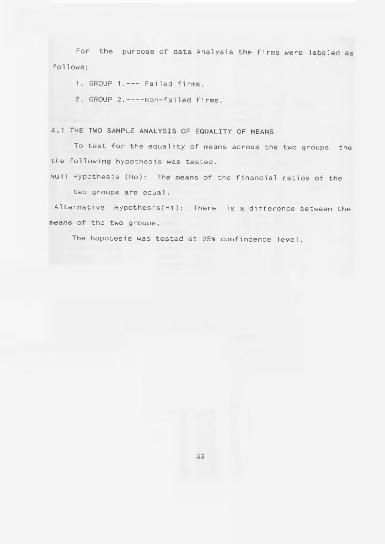
For the purpose of data Analysis the firms were labeled as
fol1ows:
1. GROUP 1.--- Failed firms.
2. GROUP 2.----Non-failed firms.
4.1 THE TWO SAMPLE ANALYSIS OF EQUALITY OF MEANS
To test for the equality of means across the two groups the
the following hypothesis was tested.
Null Hypothesis (Ho): The means of the financial ratios of the
two groups are equal.
Alternative Hypothesis(H1 ): There is a difference between the
means of the two groups.
The hopotesis was tested at 95% confindence level.
33
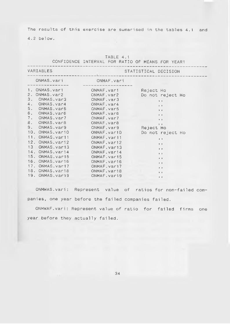
The results of this exercise are sumarised in the tables 4.1 and
4. 2 below.
TABLE 4.1CONFIDENCE INTERVAL FOR RATIO OF MEANS FOR YEAR 1
VARIABLES STATISTICAL DECISION
ONMAS.vari ONMAF.vari
1 . ONMAS.var1 ONMAF.var1 Reject Ho2. ONMAS.var2 ONMAF.var2 Do not reject Ho3. ONMAS.var3 ONMAF.var34. ONMAS.var4 ONMAF.var45. ONMAS.var5 ONMAF.var5 ) i
6. ONMAS.var6 ONMAF.var67 . ONMAS.var7 ONMAF.var78. ONMAS.var8 ONMAF.var89. ONMAS.var9 ONMAF.var9 Reject Ho10 . ONMAS.var10 ONMAF.var10 Do not reject Ho1 1. ONMAS.var11 ONMAF.var11 l l
12 . ONMAS.var12 ONMAF.var1213 ONMAS.var13 ONMAF.var13 J i
14 . ONMAS.var14 ONMAF.var1415 . ONMAS.var15 ONMAF.var1516 . ONMAS.var16 ONMAF.var161 7 . ONMAS.var17 ONMAF.var1718 . ONMAS.var18 ONMAF.var181 9 . ONMAS.var19 ONMAF.var19 } ?
ONMWAS.vari : Represent value of ratios for non-failed com-
panies, one year before the failed companies failed.
ONMWAF.vari: Represent value of ratio for failed firms one
year before they actually failed.
34
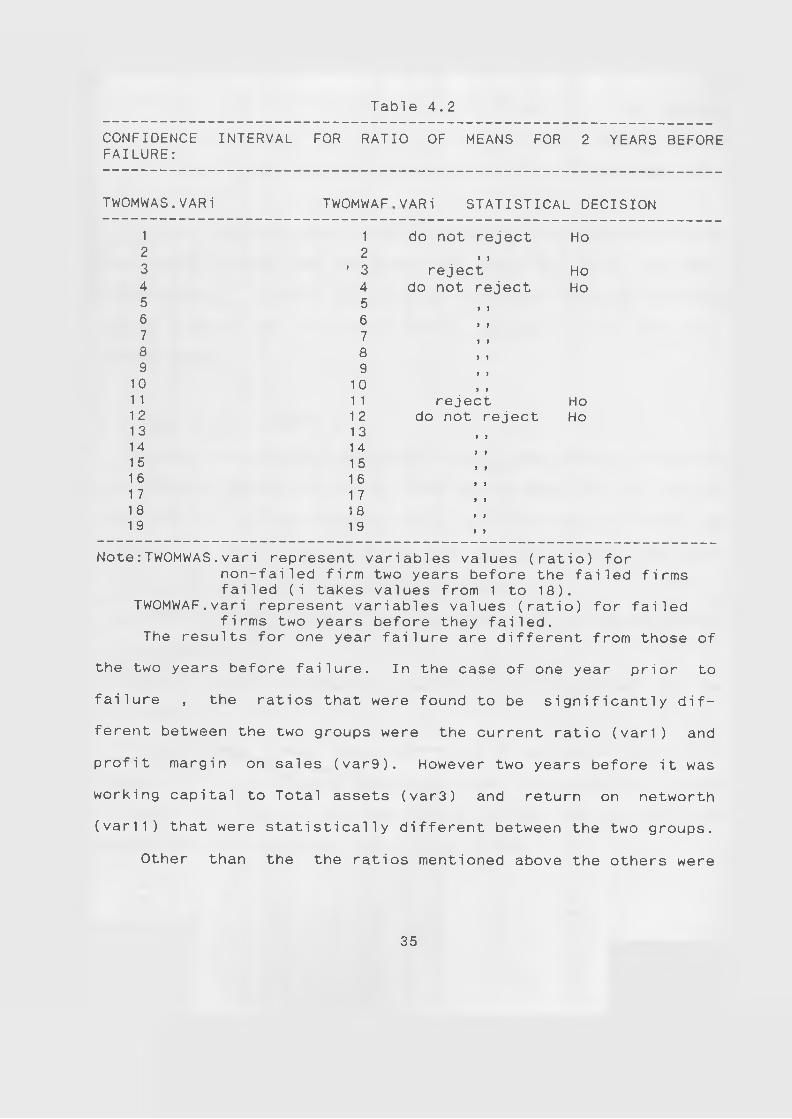
Table 4.2
CONFIDENCE INTERVAL FAILURE:
FOR RATIO OF MEANS FOR 2 YEARS BEFORE
TWOMWAS.VARi TWOMWAF VARi STATISTICAL DECISION
1 1 do not reject Ho2 2 > )3 ' 3 reject Ho4 4 do not reject Ho5 5 1 16 67 78 89 9
10 10 > )1 1 1 1 reject Ho12 1 2 do not reject Ho1 3 1314 1 41 5 1 5 l 11 6 1 61 7 1 71 8 1 81 9 1 9 1 >
Note:TWOMWAS.vari represent variables values (ratio) fornon-failed firm two years before the failed firms failed (i takes values from 1 to 18).
TWOMWAF.vari represent variables values (ratio) for failed firms two years before they failed.
The results for one year failure are different from those of
the two years before failure. In the case of one year prior to
failure , the ratios that were found to be significantly dif
ferent between the two groups were the current ratio (vari) and
profit margin on sales (var9). However two years before it was
working capital to Total assets (var3) and return on networth
(var11) that were statistically different between the two groups.
Other than the the ratios mentioned above the others were
35

found not to be significantly different between the two groups.
This is an obvious indication that a mere comparison of ratios
may be insufficient to discriminate between the failed and non-
failed fi rms.
This exercise was useful in determining important ratios
that differ between the two groups and hence may help in their
discrimination. Again the results indicate that model building
may be a better way of discriminating between failed and non-
failed fi rms.
4.2 MODEL DEVELOPMENT
Discriminant analysis was used in model development.The ratios
for one year before the failed firms failed were used to develop
the models. It was assumed that the firms characteristics (as
measured by ratios ) would differ most between failing and non
failing companies one year before failure.
The following guide-lines were used in selecting the enter
ing variables,
1. As many variables as possible were incorporated in the
fi rst model.
2. Ratios whose means were found to be statistically dif
ferent in the preliminary tests were given first priority. Hence
( based on data for one year before failure) current ratio c
profit margins were given the first priority.
36

3. Variables that were not highly correlated to any other
were given second priority the reason being they were assumed to
contain different information.
4. For the variables that were highly correlated! See appen
dix D) to others priority was given to those that had been found
to be significant in discriminating failed firms in previous
studies.
4.3 DEVELOPMENT OF MODELS
4.3.1 THE DEVELOPMENT OF THE FULL MODEL
The full model contained fifteen financial ratios! these
were the maximum number of variables that the statgraphic package
cou1d take).
The model included the following variables selected on the
basis of guidelines enumerated in section 4.2.
Table 4.3
1. ONEMW.varl ........ ........current ratio2. 0NEMW.var2 ............... quick ratio3. 0NEMW.var3.................Working capital to total debt4. 0NEMW.var4.................Equity to total liabilities5. 0NEMW.var5.................Total debt to total assets6. 0NEMW.var6.................Times interest earned7. 0NEMW.var7 ............... Fixed Charge coverage8. 0NEMW.var8.................Retained Earning to Total assets9. 0NEMW.var9.................Profit margin on sales
10. ONEMW.varlO................Return on total assets11. ONEMW.varl 1................Return on Net worth12. 0NEMW.var12................Inventory Turnover13. 0NEMW.var13................Average collection14.ONEMW.var18....... Monetary Assets to monetary liabilities15. ONEMW.var19......change in monetary liabilities
37

Since there were two groups only, a single discriminant function
was developed.20
The statistics were very impressive . The wilks lambda associated
with the function was 0.0489815. This would indicate that the
discriminant model was almost perfect. The Canonical correlation
was very high being o.97520. The eigenvalue was also
impressive(19.415866)21 The model was able to classify companies
in their respective classes 100% correctly. The resulting dis
criminant functions are as follows:
1. With standardised coefficientsZ= 6.294462var1 - 7.07647var2 + 7.90108var3 - 12.9083var4
- -2.45675var5 - 60.4844var6 + 58.9216var7 + 5.14276var8-1.17486var9 + 0.08290var10 + 0.60747var11 + 1.20046var12- 0.54801var13 + 0.02162var18 + 2.85340var19
20. The number of discriminant functions is equal to the number of groups
minus one or the number of independent variables whichever is
smal1(Peterson,1982:541). In this case the number of groups 2-1= 1
21. Wilk lambda is a measure of dicriminating power not already accounted for
by the model(the smaller it is the better). Canonical correlation is a statis
tical measure of discriminating power already in the model (the bigger it is
the better). The eigenvalue is a measure of relative importance of a
function(The bigger it is the better).
38

2. With unstandardised coefficients1- 1.65451var1 - 1.92102var2 + 4.26715var3 - 6.52455var4
- 9.12535var5 - 1.67719var6 + 1.69460var7 + 34.2580var8- 7.80731var9 + 0.4961var10 + 0.07733var11+ 0.26294var12 - 0.00268var13 + 0.07661var18- 4.87930var19 + 7.60642
Where Z-represents the discriminant score
vari- represent the ith financial ratio for the year before
failure occurred.
i = 1,2,..., 19.
It can be observed from the disciminant function that the
ratios can be ranked as follows in order of discriminating
power(based on the standardised coefficients).
TABLE 4.4
THE FULL MODEL RANKS BASED ON DISCRIMINANT POWER
RANK RATIO VARIABLEPOSITION
1 . Times interest earned var62 . Fixed Charge coverage var73. Equity to total liabilities var44. Working capital .to total debt var35 . Quick ratio var26. Current ratio var 17 . Retained earning to total assets var88. Change in monetary liabilities var 1 99. Total debt to total assets var5
10. Inventory Turnover var 1 21 1 . Profit margin on sales var912. Return on net worth var 1 113. Average collection period var 1 314. Return on total assets var 1 015. Monetary assets to monetary liabilities var 1 8
39
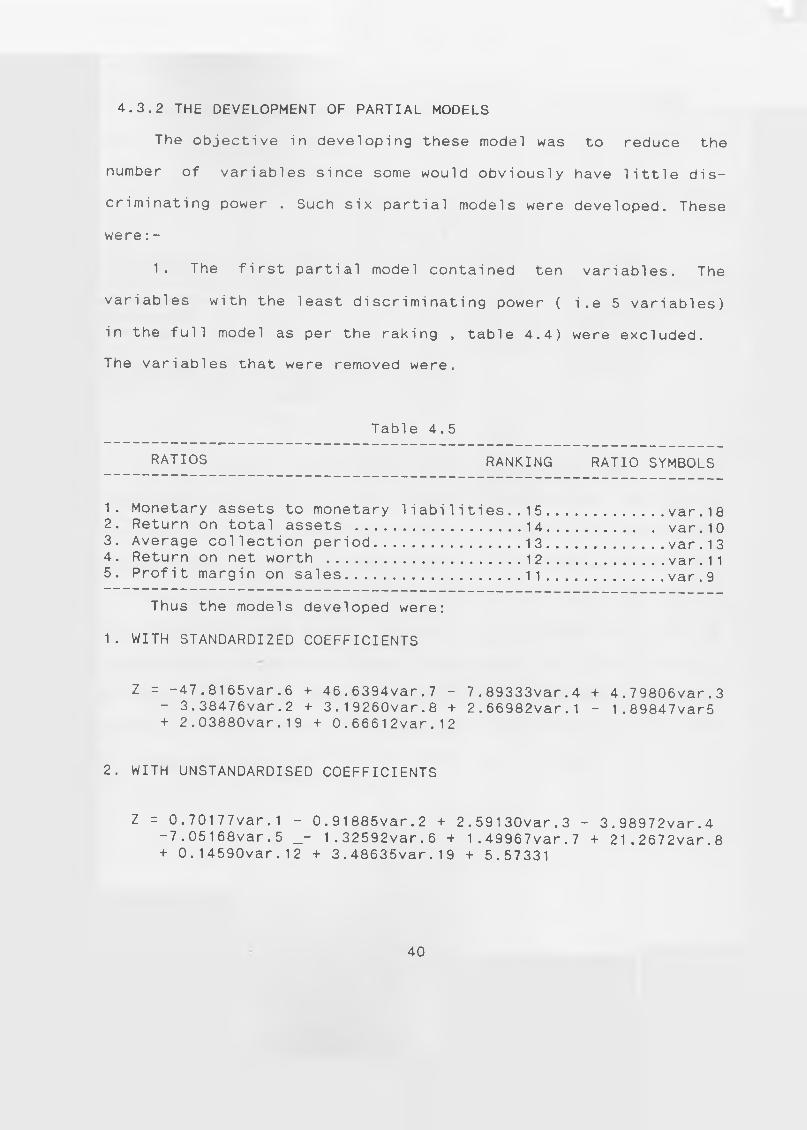
4.3.2 THE DEVELOPMENT OF PARTIAL MODELS
The objective in developing these model was to reduce the
number of variables since some would obviously have little dis
criminating power . Such six partial models were developed. These
were:-
1. The first partial model contained ten variables. The
variables with the least discriminating power ( i.e 5 variables)
in the full model as per the raking , table 4.4) were excluded.
The variables that were removed were.
Table 4.5
RATIOS RANKING RATIO SYMBOLS
1 . 2 .3.4.5.
Monetary assets to monetary liabilities..Return on total assets ....................Average collection period..................Return on net worth ........................Profit margin on sales.....................
15.............. var . 1 814............. var.1013.............. var . 1 312.............. var . 1 111.............. var . 9
Thus the models developed were:
1. WITH STANDARDIZED COEFFICIENTS
Z = -47.8165var.6 + 46.6394var.7 - 7.89333var.4 + 4.79806var.3 - 3.38476var.2 + 3.19260var.8 + 2.66982var.1 - 1.89847var5 + 2.03880var.19 + 0.66612var.12
2. WITH UNSTANDARDISED COEFFICIENTS
Z = 0.70177var.1 - 0.91885var.2 + 2.59130var.3 - 3.98972var.4 -7.05168var.5 _- 1.32592var.6 + 1.49967var.7 + 21.2672var.8 + 0.14590var.12 + 3.48635var.19 + 5.57331
40
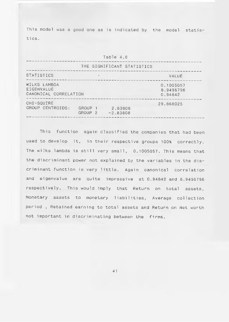
This model was a good one as is indicated by the model statis-
tics.
Table 4.6
THE SIGNIFICANT STATISTICS
STATISTICS » VALUE
WILKS LAMBDA EIGENVALUECANONICAL CORRELATION
0.10050578.94967960.94842
CHI-SQUIRE GROUP CENTROIDS: GROUP 1
GROUP 22.83808
-2.83808
29.868025
This function again Classified the companies that had been
used to develop it, in their respective groups 100% correctly.
The wilks lambda is still very small, 0.1005057. This means that
the discriminant power not explained by the variables in the dis
criminant function is very little. Again canonical correlation
and eigenvalue are quite impressive at 0.94842 and 8.9496796
respectively. This would imply that Return on total assets,
Monetary assets to monetary liabilities, Average collection
period , Retained earning to total assets and Return on Net worth
not important in discriminating between the firms.
41
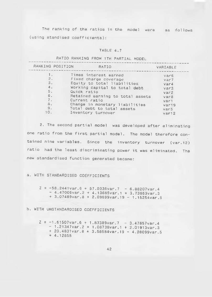
The ranking of the ratios in the model were as foilows
(using standised coefficients):
TABLE 4.7
RATIO RANKING FROM 1TH PARTIAL MODEL
RANKING POSITION RATIO VARIABLE
1 . Times interest earned var62 # Fixed charge coverage var73. Equity to total liabilities var44. Working capital to total debt var35. Quick ratio var26. Retained earning to total assets var87 . Current ratio var 18. Change in monetary liabilities var 1 99 . Total debt to total assets var5
10. Inventory turnover var 1 2
2. The second partial model was developed after eliminating
one ratio from the first partial model. The model therefore con
tained nine variables. Since the inventory turnover (var.12)
ratio had the least discriminating power it was eliminated. The
new standardised function generated became:
a. WITH STANDARDISED COEFFICIENTS
Z = -58.2441var.6 + 57.0336var.7 - 6.88207var.4- 4.47006var.2 + 4.13685var.1 + 3.73863var.3 + 3.07489var.8 + 2.09699var.19 - 1.15254var.5
b. WITH UNSTANDARDISED COEFFICIENTS
Z = - 1 .61507var.6 + 1.83389var.7 - 3.47857var.4- 1.21347var.2 + 1.08738var.1 + 2.01913var.3 + 20.4831var.8 + 3.58584var.19 - 4.28099var.5 + 4.12855
42
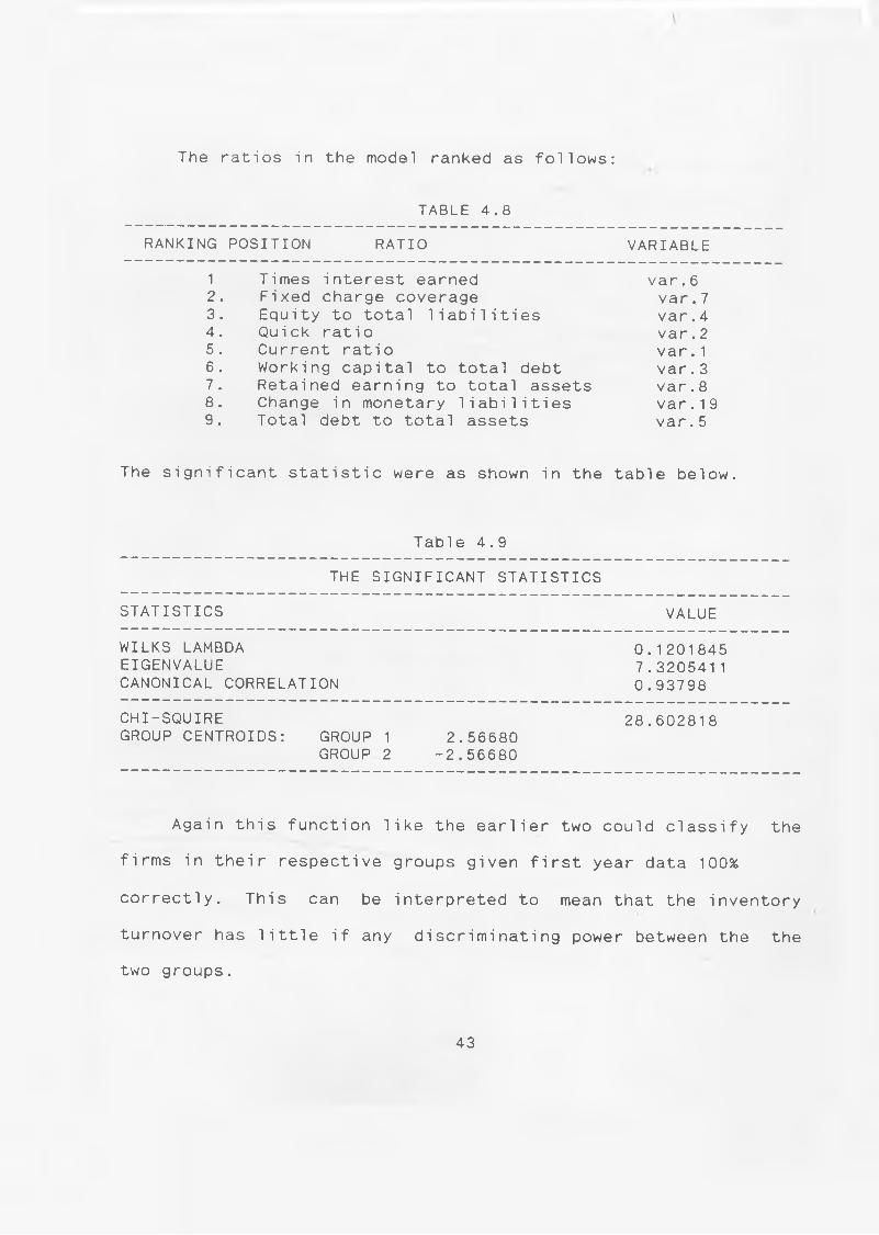
The ratios in the model ranked as follows:
TABLE 4.8
RANKING POSITION RATIO VARIABLE
1 Times interest earned var. 62. Fixed charge coverage var. 73. Equity to total liabilities var. 44 . Quick ratio var. 25 . Current ratio var. 16 . Working capital to total debt var. 37 . Retained earning to total assets var. 88. Change in monetary liabilities var.199. Total debt to total assets var. 5
The significant statistic were as shown in the table below.
Table 4.9
THE SIGNIFICANT STATISTICS
STATISTICS VALUE
WILKS LAMBDA EIGENVALUECANONICAL CORRELATION
0.1201845 7.3205411 0.93798
CHI-SQUIRE GROUP CENTROIDS: GROUP
GROUP1 2.566802 -2.56680
28.602818
Again this function like the earlier two could classify the
firms in their respective groups given first year data 100%
correctly. This can be interpreted to mean that the inventory
turnover has little if any discriminating power between the the
two groups.
43
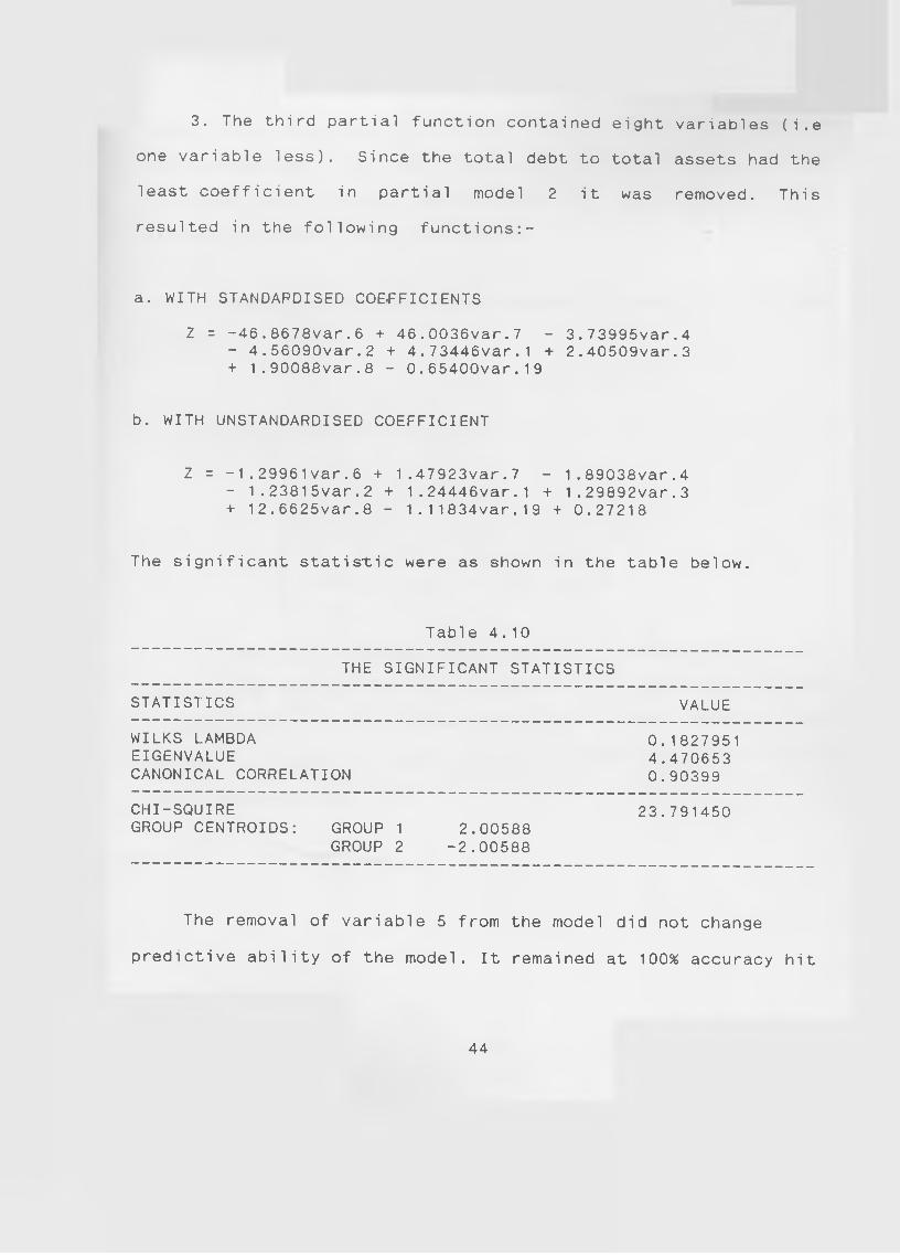
3. The third partial function contained eight variables (i.e
one variable less). Since the total debt to total assets had the
least coefficient in partial model 2 it was removed. This
resulted in the following functions:-
a. WITH STANDARDISED COE-FFICIENTS
Z = -46.8678var.6 + 46.0036var.7 - 3.73995var.4- 4.56090var.2 + 4.73446var.1 + 2.40509var.3 + 1.90088var.8 - 0.65400var.19
b. WITH UNSTANDARDISED COEFFICIENT
Z = - 1 .29961var.6 + 1.47923var.7 - 1.89038var.4- 1.23815var.2 + 1.24446var.1 + 1.29892var.3 + 12.6625var.8 - 1.11834var.19 + 0.27218
The significant statistic were as shown in the table below.
Tab!e 4.10
THE SIGNIFICANT STATISTICS
STATISTICS VALUE
WILKS LAMBDA EIGENVALUECANONICAL CORRELATION
0.18279514.4706530.90399
CHI-SQUIREGROUP CENTROIDS: GROUP 1 2.00588
GROUP 2 -2.00588
23.791450
The removal of variable 5 from the model did not change
predictive ability of the model. It remained at 100% accuracy hit
44
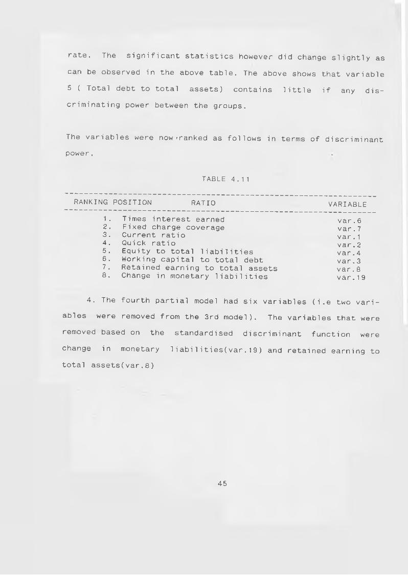
rate. The significant statistics however did change slightly as
can be observed in the above table. The above shows that variable
5 ( Total debt to total assets) contains little if any dis
criminating power between the groups.
The variables were now-ranked as follows in terms of discriminant
power.
TABLE 4.11
RANKING POSITION RATIO VARIABLE
1. Times interest earned var.62. Fixed charge coverage var.73. Current ratio var.14. Quick ratio var.25. Equity to total liabilities var.46. Working capital to total debt var.37. Retained earning to total assets var.88. Change in monetary liabilities var.19
4. The fourth partial model had six variables (i.e two vari
ables were removed from the 3rd model). The variables that were
removed based on the standardised discriminant function were
change in monetary 1iabi1ities(var.19) and retained earning to
total assets(var.8)
45
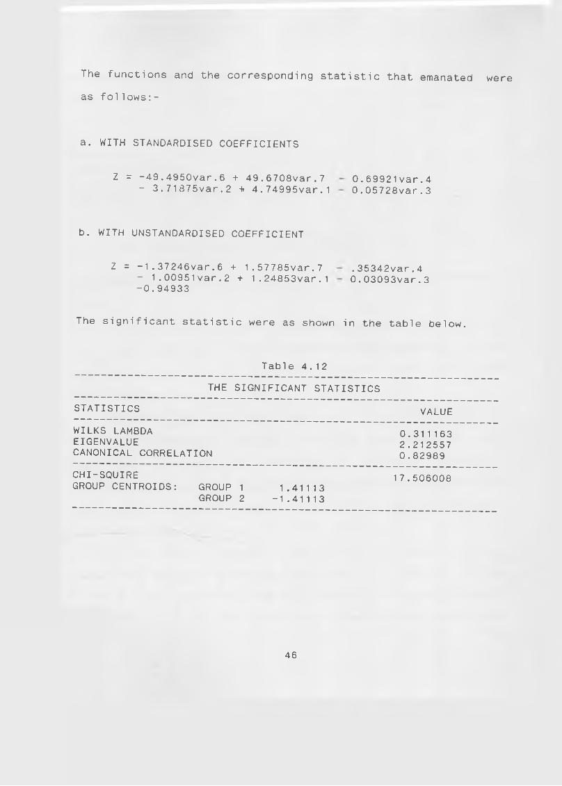
The functions and the corresponding statistic that emanated
as foilows:-
were
a. WITH STANDARDISED COEFFICIENTS
2 = -49.4950var.6 + 49.6708var.7 - 3.71.875var.2 + 4.74995var.1
0.69921var.4 0.05728var.3
b. WITH UNSTANDARDISED COEFFICIENT
Z = -1.37246var.6 + 1.57785var.7 - 1.00951var.2 + 1.24853var.1 -0.94933
.35342var.4 0.03093var.3
The significant statistic were as shown in the table below.
Table 4.12
THE SIGNIFICANT STATISTICS
STATISTICS VALUE
WILKS LAMBDA EIGENVALUECANONICAL CORRELATION
0.311163 2.212557 0.82989
CHI-SQUIREGROUP CENTROIDS: GROUP 1 1.41113
GROUP 2 -1.41113
17.506008
46
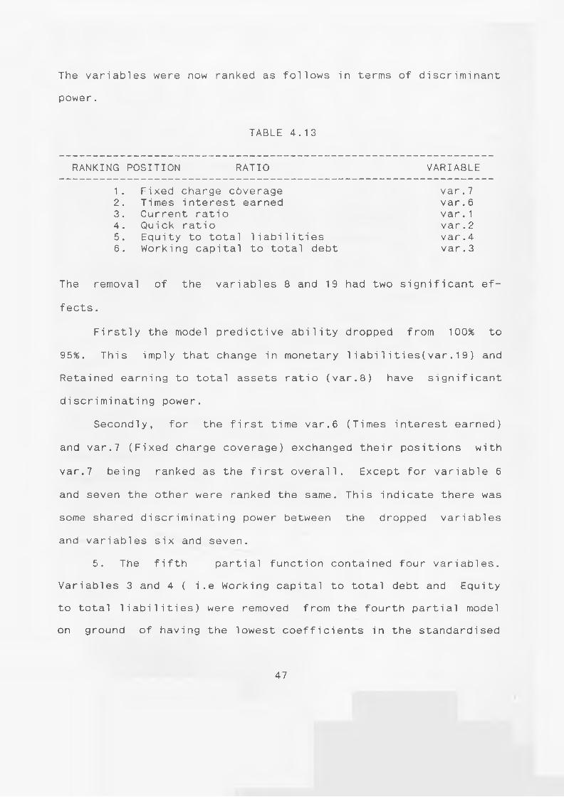
The variables were now ranked as follows in terms of discriminant
power.
TABLE 4.13
RANKING POSITION RATIO VARIABLE
1 . Fixed charge cdverage var. 72 . Times interest earned var. 63 . Current ratio var. 14 . Quick ratio var. 25 . Equity to total liabilities var. 46 . Working capital to total debt var. 3
The removal of the variables 8 and 19 had two significant ef
fects.
Firstly the model predictive ability dropped from 100% to
95%. This imply that change in monetary 1iabi1ities(var.19) and
Retained earning to total assets ratio (var.8) have significant
discriminating power.
Secondly, for the first time var.6 (Times interest earned)
and var.7 (Fixed charge coverage) exchanged their positions with
var.7 being ranked as the first overall. Except for variable 6
and seven the other were ranked the same. This indicate there was
some shared discriminating power between the dropped variables
and variables six and seven.
5. The fifth partial function contained four variables.
Variables 3 and 4 ( i.e Working capital to total debt and Equity
to total liabilities) were removed from the fourth partial model
on ground of having the lowest coefficients in the standardised
47
model.
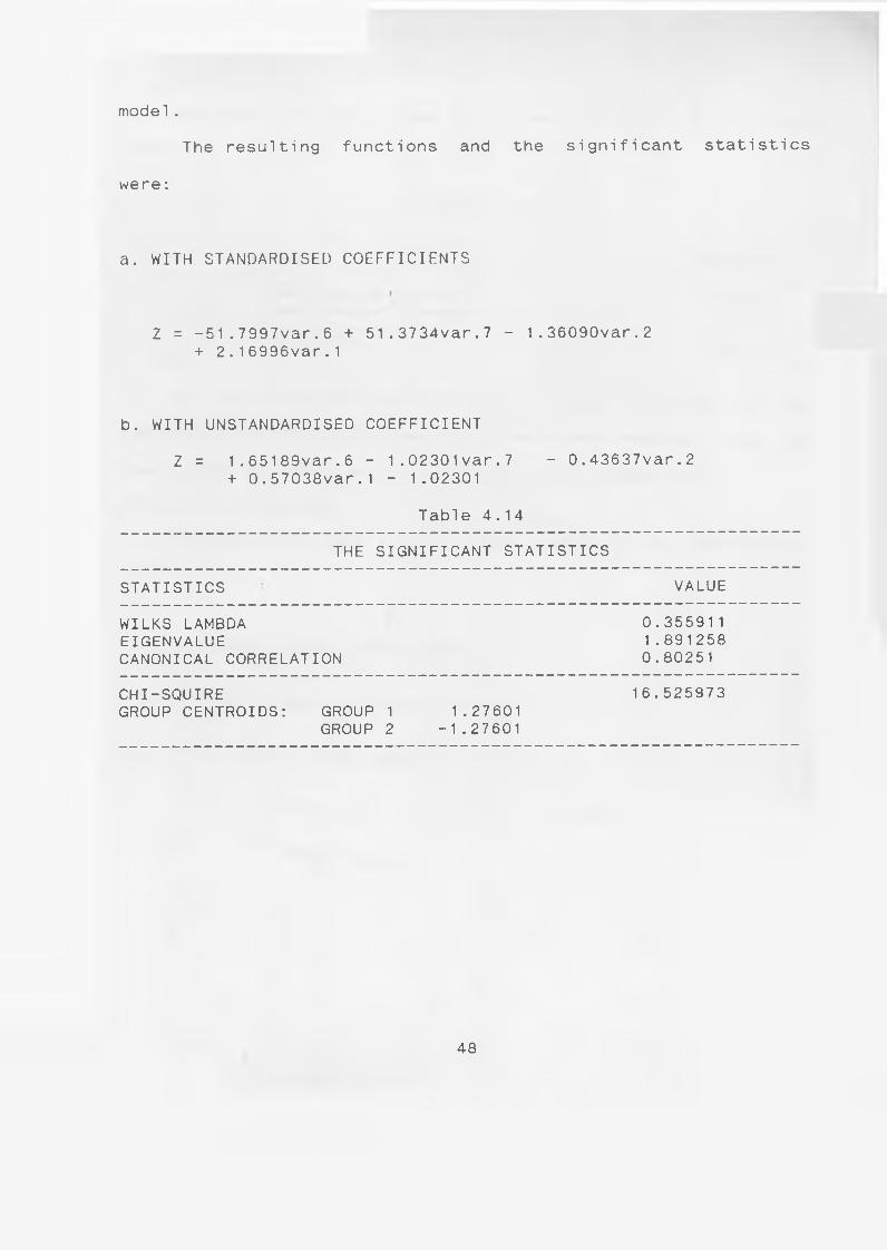
The resulting functions and the significant statistics
were:
a. WITH STANDARDISED COEFFICIENTS
Z = -51.7997var.6 + 51.3734var.7 - 1.36090var.2 + 2.16996var.1
b. WITH UNSTANDARDISED COEFFICIENT
Z = 1.65189var.6 - 1.02301var.7 - 0.43637var.2+ 0.57038var.1 - 1.02301
Table 4.14
THE SIGNIFICANT STATISTICS
STATISTICS VALUE
WILKS LAMBDA EIGENVALUECANONICAL CORRELATION
0.355911 1.891258 0.80251
CHI-SQUIREGROUP CENTROIDS: GROUP 1
GROUP 21 .27601
-1.27601
16.525973
48
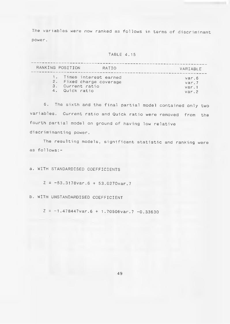
The variables were now ranked as To!lows in terms of discriminant
power.
TABLE 4.15
RANKING POSITION RATIO VARIABLE
1. Times interest earned2. Fixed charge coverage3. Current ratio4. Quick ratio
var. 6 var. 7 var. 1 var. 2
6. The sixth and the final partial model contained only two
variables. Current ratio and Quick ratio were removed from the
fourth partial model on ground of having low relative
discriminanting power.
The resulting models, significant statistic and ranking were
as foilows:-
a. WITH STANDARDISED COEFFICIENTS
Z = -53.3178var.6 + 53.0270var.7
b. WITH UNSTANDARDISED COEFFICIENT
Z = -1.478447var.6 + 1.70506var.7 -0.33630
49
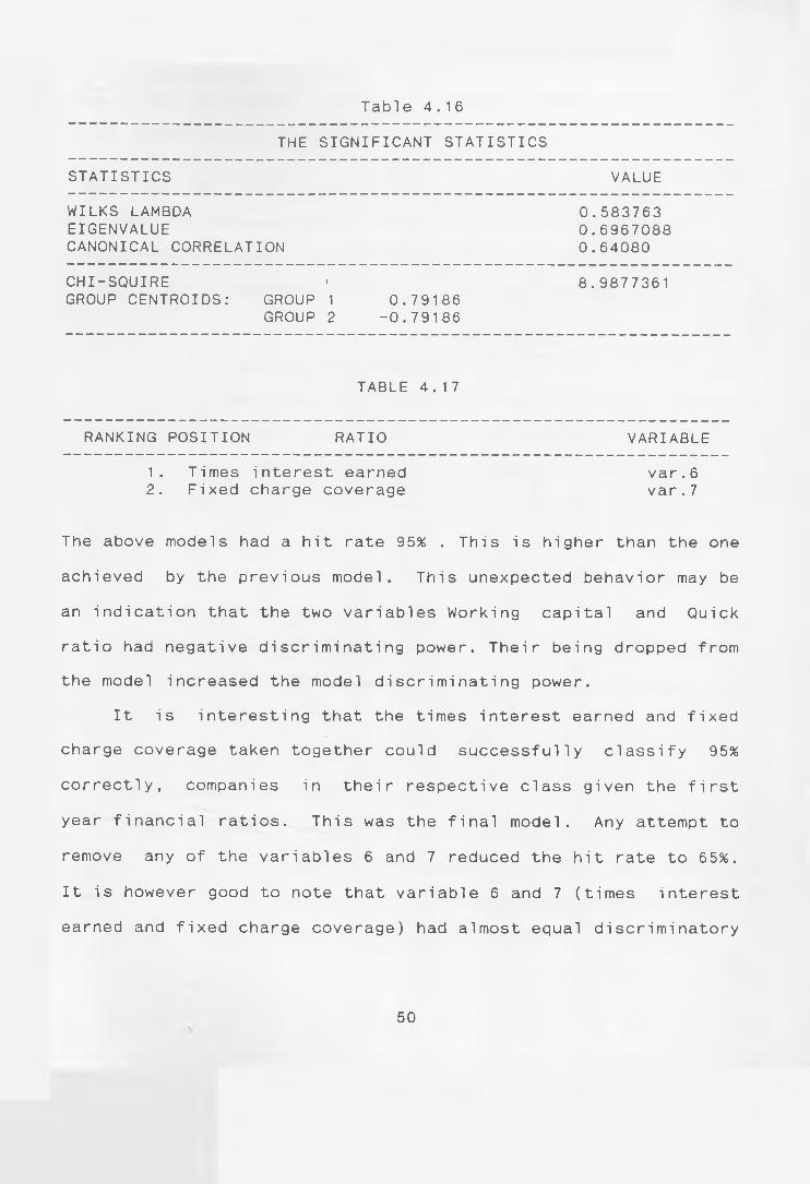
Table 4.16
THE SIGNIFICANT STATISTICS
STATISTICS VALUE
WILKS LAMBDA EIGENVALUECANONICAL CORRELATION
0.5837630.69670880.64080
CHI-SQUIRE GROUP CENTROIDS: GROUP
GROUP
11 0.791862 -0.79186
8.9877361
TABLE 4.17
RANKING POSITION RATIO VARIABLE
1. Times interest earned var.62. Fixed charge coverage var.7
The above models had a hit rate 95% . This is higher than the one
achieved by the previous model. This unexpected behavior may be
an indication that the two variables Working capital and Quick
ratio had negative discriminating power. Their being dropped from
the model increased the model discriminating power.
It is interesting that the times interest earned and fixed
charge coverage taken together could successfully classify 95%
correctly, companies in their respective class given the first
year financial ratios. This was the final model. Any attempt to
remove any of the variables 6 and 7 reduced the hit rate to 65%.
It is however good to note that variable 6 and 7 (times interest
earned and fixed charge coverage) had almost equal discriminatory
50
power. Each alone when used could correctly classify companies in
their respective class 65% correctly.
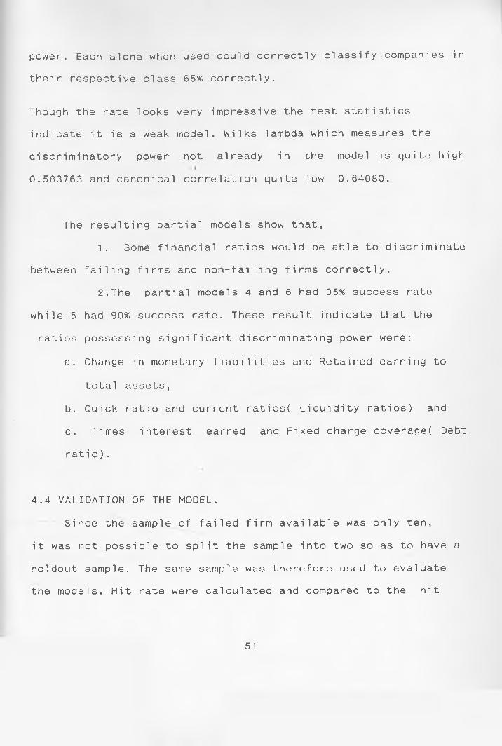
Though the rate looks very impressive the test statistics
indicate it is a weak model. Wilks lambda which measures the
discriminatory power not already in the model is quite high
0.583763 and canonical correlation quite low 0.64080.
The resulting partial models show that,
1. Some financial ratios would be able to discriminate
between failing firms and non-failing firms correctly.
2. The partial models 4 and 6 had 95% success rate
while 5 had 90% success rate. These result indicate that the
ratios possessing significant discriminating power were:
a. Change in monetary liabilities and Retained earning to
total assets,
b. Quick ratio and current ratios( Liquidity ratios) and
c. Times interest earned and Fixed charge coverage( Debt
ratio).
4.4 VALIDATION OF THE MODEL.
Since the sample of failed firm available was only ten,
it was not possible to split the sample into two so as to have a
holdout sample. The same sample was therefore used to evaluate
the models. Hit rate were calculated and compared to the hit
51

rates of the other models and chance2 2 . The higher the hit rate
the better the model.
In total 7 models were developed. These were:
1. full model (w i th 15 variables )
2. parti al model 1 (with 10 variables)
3. partial model 2 (with 9 variables)
4 . partial model 3 (with 8 variables)
5. partial model 4 (with 6 variables)
6 . partial model 5 (with 4 variables)
7 . partial model 6 (with 2 variables)
22. Since the sample sizes are equal the probability of a company belonging to
any group is 50%
52
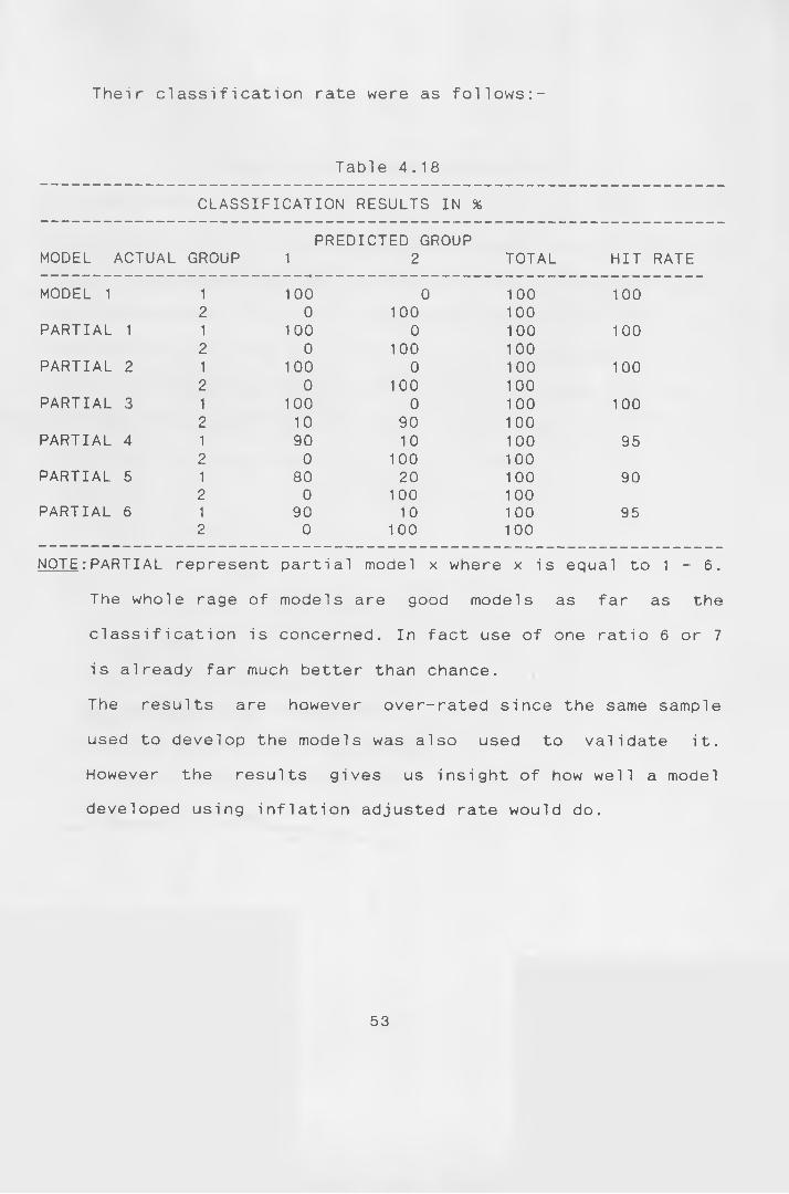
Their classification rate were as follows:-
Table 4.18
CLASSIFICATION RESULTS IN %
PREDICTED GROUPMODEL ACTUAL GROUP 1 2 TOTAL HIT RATE
MODEL 1 1 100 0 100 1002 0 100 100
PARTIAL 1 1 100 0 100 1002 0 100 100
PARTIAL 2 1 100 0 100 1002 0 100 100
PARTIAL 3 1 100 0 100 1002 10 90 100
PARTIAL 4 1 90 10 100 952 0 100 100
PARTIAL 5 1 80 20 100 902 0 100 1 00
PARTIAL 6 1 90 10 100 952 0 100 100
NOTE:PARTIAL represent partial model x where x is equal to 1 - 6.
The whole rage of models are good models as far as the
cl ass i f i cation i s concerned. In fact use of one ratio 6 or 7
is already far much better than chance.
The results are however over-rated since the same sample
used to develop the models was also used to validate it.
However the results gives us insight of how well a model
developed using inflation adjusted rate would do.
53

CHAPTER 5
CONCLUSIONS AND RECOMMENDATIONS
5.1 CONCLUSIONS
Stake holders in firms are interested in corporate survival.
However corporations do fail leading to untold suffering to all
the stake holders. This has brought about the concern for
corporate failure. The study set to investigate the ability of
the inflation adjusted accounts to predict corporate failure.
The following ratios are ranked in the order of
discriminating power, beginning with the best:-
1. Times interest coverage.
2. Fixed charge coverage.
3. Equity to total liabilities.
4. Quick ratio .
5. Current ratio.
6. Working capital to total debt.
7. Retained earning to total assets.
8. Change in monetary liabilities.
9. Total debt to total assets.
54
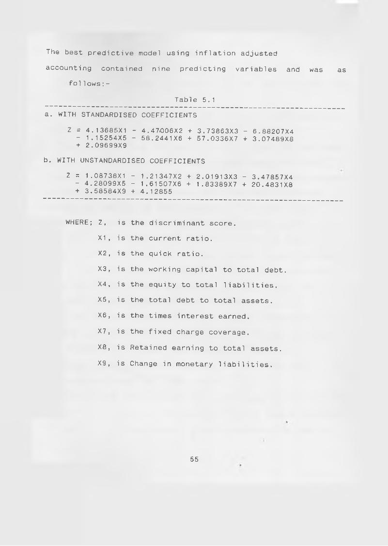
The best predictive model using inflation adjusted
accounting contained nine predicting variables and was
fol1ows:-
Table 5.1
a. WITH STANDARDISED COEFFICIENTS
Z = 4.13685X1 - 4.47.006X2 + 3.73863X3 - 6.88207X4- 1.15254X5 - 58.2441X6 + 57.0336X7 + 3.07489X8+ 2.09699X9
b. WITH UNSTANDARDISED COEFFICIENTS
Z = 1.08738X1 - 1.21347X2 + 2.01913X3 - 3.47857X4- 4.28099X5 - 1.61507X6 + 1.83389X7 + 20.4831X8+ 3.58584X9 + 4.12855
WHERE; Z, is the discriminant score.
X 1 , is the current ratio.
X 2 , is the quick ratio.
X3, is the working capital to total debt.
X 4 , is the equity to total liabilities.
X5, is the total debt to total assets.
X 6 , is the times interest earned.
X7 , is the fixed charge coverage.
X8, is Retained earning to total assets.
X 9 , is Change in monetary liabilities.
as
55
The findings provides evidence that;
1. Inflation adjusted accounting can be used for predicting
failure.
2. One Should concentrate on the above ratios if there was need
to forecast firm’s survival.
3. Most firms in kenya fail due to the poor funds flow management
and unwise debt policies. The most critical ratios were the
liquidity ratios (i.e current and quick ratios) and debt coverage
ratios (i.e Times interest earned and Fixed charge coverage
ratios. The results are thus consistent with finance theory
relating to the firms risk. The firm must maintain sufficient
liquidity if it is to avoid insolvency problems. It must also
generate sufficient earnings to meet its fixed finance charges
(specifically interest). Inadequate liquidity and low earning
relative to fixed finance charges are the best signals for
impending failure in the kenyan environment.
The results however differ from earlier studies into the
subject by Altman (1968) and kimura (1982) who had concluded
that liquidity ratios were not of any significance in
bankruptcy prediction. Both concluded that efficiency and
profitability ratios were most crucial.
The results of this study thus gives support to the existing
finance theory that risk considerations are of immense importance
in mode mporate management. Though accounting data may be
56
manipulated by the management, when adjusted for price-level
changes it provides fantastic forecasting capabilities.
5.2 RECOMMENDATIONS OF THE STUDY
The results of this study indicate that most companies in
kenya fail due to poor funds flow management and unwise debt
decisions.
Managers therefore should intelligently manage funds or
working capital ensuring that sufficient liquidity is available
all the time. Most important, managers should realise that
failure results from inability to service debt and other related
fixedfinancial charges. This is a clear indicator that the
managers are not investing in high return projects and therefore
calls for either a more careful evaluation of investments before
plugging in more resource or more efficient utilization of
resources.
Managers should therefore be willing to adopt modern
management techniques which impinge on efficiency. Otherwise they
should avoid using debt finance and opt for more expensive but
less risky equity finance. Since the capital structure ratios
were not found to be significant then the problem of inability to
service debt cannot be attributed to excessive use of debt, the
truth is that investment returns are simply not satisfactory.
57
5.3 LIMITATIONS OF THE STUDY
Results of this study should be interpreted in the light
of the following limitations;
1. The validation results from the confusion matrix are biased
upwards because the same lObservations used to develop the model
were used to test the model.
2. The sample size used here is small and therefore the model is
not stable. The coefficient would most probably change if a large
sample was used. The sample size is no doubt this study’s
severest drawback.
3. It was not possible to calculate some ratios from the
available financial statements owing to the fact that most
companies give the minimum legal disclosures which have been
found wanting. The publicly available information was inadequate
to provide the data needed for this kind of study.
4. Financial ratios generated from financial statements cannot be
better than data from which they are based. The study is
therefore constrained by the limitations of financial statement
preparation.
5. Financial data is only one source of signal about corporate
failure. In reality other non-quantifiable circumstances and
reasons could lead to failure. Examples are the catastrophes
and exogenous considerations.
58

5.4 DIRECTIONS FOR FUTURE RESEARCH
i. This study used the GDP deflator for adjustment pur
poses. Other price adjustment study index numbers like the
specific price index could be used to develop a similar
model. 1
ii. This study considered only price adjusted data. A study
testing the superiority of Historical cost and price level
adjusted data ought to be done.
iii. This study could be varied so as to enable the use of
Stepwise discriminant analysis.
BIBLIOGRAPHY
Accounting Standard Committee Statement of Standard Accounting
Practice No. 16 ; Current Cost Accounting, London , 1980
Altman I, "Financial Ratios,Discriminant Analysis And the Pre
diction of corporate B a n k r u p t c y Journal of finance.Volume xxiii
September no 4 1968.
ALtman, E. I , R. G. Haldeman and P. Narayan, "Zeta Analysis: A
New Model to Identify Bankruptcy Risk of Corporation, Journal of
Finance and Baking , Vol. 1, No. 1, 1977.
Altman E. and Mcough, Evaluation of a company as a going con
cern, Journal of accounting. December 1974.
American Accounting Association, "Report of the Committee on Ac
counting Valuation Basis", Supplement to The Accounting Review,
1972.
Baron,Aron J., Lakonishok and A. R. Ofer "The Information Content
Of Price Level Adjusted EarningrSome Empirical Evidence."The ac
counting Review. January 1980.
60

Beaver W.H, "Alternative Accounting Measures As Predictors Of
Failure", Accounting Review. January 1968 , pg113 - 122
Blum M, "Failing Company Discriminant Analysis".Journal of Ac
countancy And Research .Spring.1974. pp 1 - 25
Chambers, Raymond J. "Accounting Evaluation and Economic
Behavior", Prentice-hall, 1966.
Dambolena G. and Khoury, "Ratio Stability And Corporate
Fai1ure".Journal Of Finance.Vol xxxv.No. 4.September 1980 p g .
1017 -1027.
Dambolena , Usmael G. , and s. J. Khoury, " Ratio Stability and
Corporate Failure", The Journal of Finance. September 1980.
Davidson , Sidney and Roman L. Weil, "Inflation Accounting: What
Will General Price Level Adjustment Income Statement Show?’
Financial Analysts Journal. Jan /Feb, 1975.
Dyckman, Thomas R. , "Investment Analysis And General Price Level
Adjustment", American Accounting Association, 1969.
61
Edward E .W Investment Analysis" ,Prentice Hall Inc,1974 pg 115
130
George F o s t e r Financial Statement Analysis " .prentice Hall, In
I
____________, " Market Prices,Financial Ratios And The Prediction
Of Fai1u r e Journal Of Accounting Research.Spring 1974 pg 1 - 25
Gilbert L, and B.Kenneth, "Prediction Of Bankruptcy For Firms In
Financial Pi stress",Journal Of Business And Accounting.Spring
1990
Ijiri and Jaedieke,"The Objectivity and Reliability Of Accounting
Measurements".The Accounting Review July 1966
Jensen and Meckling
Slautier and Underdown."Accounting Theory and Practice" Pitman
1976
Kimura J.H,"The Predictive Accuracy Of Accounting and Non Ac
counting Information Under Inflationary Conditions".Unpublished
Phd Dissertation.University Of Califonia,Los Angeles.
62

Koh and Killouh, "The use of Multiple Discriminant Analysis In
The Assessment Of The Going Concern Status Of An Audit
Client",Journal Of Business Finance and Accounting .1990.d p 179
191 .
I
Littleton, A. C. And Zimmerman, V. K. "Accounting Theory
:Continuity and Change” , Prentice-hall, Englewood Cliffs, N.J.,
1 962.
Mckenzie, Patrick B. " Inflation and Financial Ratios: The Effect
of the Stable Dollar Assumption, " Review of Business And
Economic Research. Spring, 1975.
Tamari M, "Financial Ratios As A Means Of Predicting
Bankruptcy", Management International Review.Vol 4,1966,pg 15 -
21 .
Weston and Cope 1 and,"Managerial Finance" ,NewYork 1986
63

APPENDIX A
SAMPLE OF THE NON-FAILED COMPANIES
I
1 . AFRICAN TOURS AND HOTELS
2. EAST AFRICAN PORTLAND CEMENT CO. LIMITED
3. KENYA OIL COMPANY LIMITED
4. KENYA FINANCE CORPORATION LIMITED
5. KENSTOCK LIMITED
6. BABURI PORTLAND CEMENT COMPANY LIMITED
7. MALEVE AUTOMABILE AND GENERAL EQUIPMENT LIMITED
8. EAST AFRICAN CABLES LIMITED
9. ELIOTS BAKERIES LIMITED
10 MUTETI TRANSPORTERS
NOTE: The sample names of the failed companies is withheld.
64
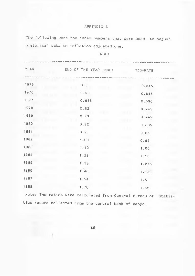
APPENDIX B
The following were the index numbers that were used to adjust
historical data to inflation adjusted one.
INDEX
YEAR1
END OF THE YEAR INDEX MID-RATE
1975 0.5 0.545
1976 0.59 0.645
1977 0.655 0.690
1978 0.82 0.745
1 989 0.79 0.745
1980 0.82 0.805
1881 0.9 0.86
1 982 1 .00 0.95
1 983 1.10 1 .05
1 984 1 .22 1.16
1 985 1 .33 1 .275
1986 1 .46 1.139
1887 1 . 54 1 . 5
1988 1 . 70 1 .62
Note: The ratios were calculated from Central Bureau of
tics record collected from the central bank of kenya.
65
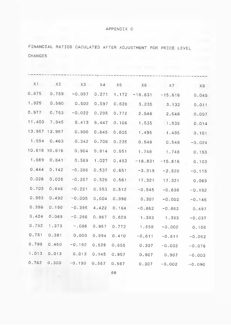
APPENDIX C
FINANCIAL RATIOS CACULATED AFTER ADJUSTMENT FOR PRICE LEVEL
CHANGES
X1 X2 X3 X4 X5 X6 X7 X8
0.875 0.769 -0.097 0.271 1.172 -18.831 -15.616 0.045
1 .925 0.580 0.502 0.597 0.626 3.235 3.132 0.011
0.977 0.753 -0.022 0.295 0.772 2.548 2.548 0.007
11.400 7.945 8.413 8.447 0.106 1 . 535 1 . 535 0.014
13.957 13.957 0.900 0.645 0.605 1.495 1 .495 0.161
1 . 554 0.463 0.342 0.708 0.235 0.548 0.548 -0.024
10.616 10.616 0.904 0.814 0.551 1.748 1 .748 0.150
1 . 569 0.841 0.569 1 .027 0.493 -18.831 -15.616 0.103
0.444 0.142 -0.386 0.537 0.651 -3.319 -2.528 -0.115
0.026 0.026 -0.257 0.526 0.561 17.321 17.321 0.069
0.703 0.646 -0.221 0.953 0.512 -0.545 -0.838 -0.192
0.993 0.492 -0.005 0,004 0.996 0.307 -0.002 -0.145
0.398 0.190 -0.395 4.422 0.184 -0.862 -0.862 0.497
0.424 0.089 -0.266 0.967 0.629 1 . 393 1 . 393 -0.037
0.792 1 .373 -.086 0.967 0.772 1.558 -0.002 0.106
0.751 0.381 0.000 0.994 0.410 -0.611 -0.611 -0.052
0.799 0.460 -0.192 0.526 0.655 0.307 -0.002 -0.076
1.013 0.013 0.013 0.145 0.957 0.907 0.907 -0.003
0.762 0.300 -0.190 0.567 0.567 0.307 -0.002 -0.090
66
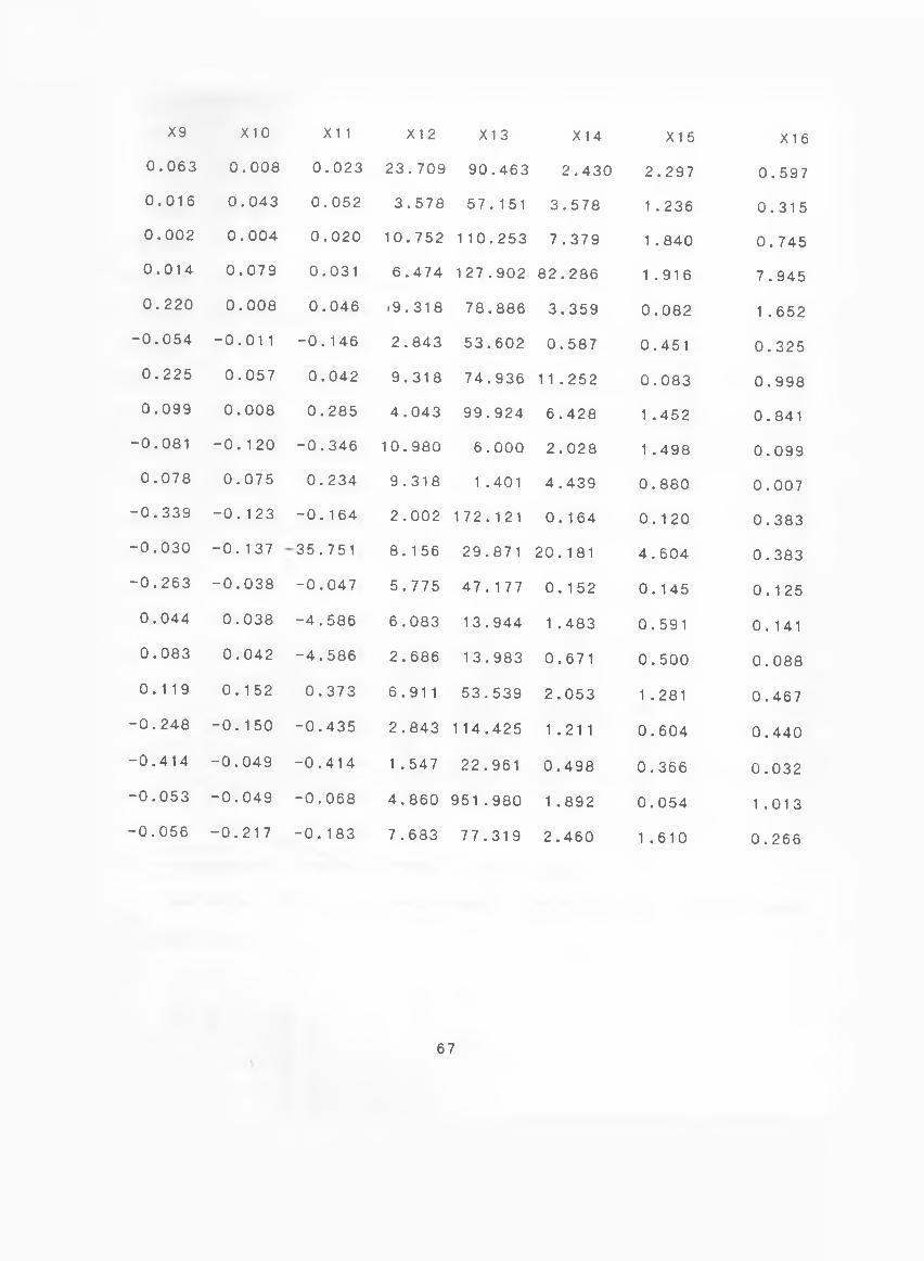
X9 X10
0.063 0.008
0.016 0.043
0.002 0.004
0.014 0.079
0.220 0.008
-0.054 -0.011
0.225 0.057
0.099 0.008
-0.081 -0.120
0.078 0.075
-0.339 -0.123
-0.030 -0.137
-0.263 -0.038
0.044 0.038
0.083 0.042
0.119 0.152
-0.248 -0.150
-0.414 -0.049
-0.053 -0.049
-0.056 -0.217
X1 1 X 1 2
0.023 23.709
0.052 3.578
0.020 10.752
0.031 6.474
0.046 -9.318
-0.146 2.843
0.042 9.318
0.285 4.043
-0.346 10.980
0.234 9.318
-0.164 2.002
35.751 8.156
-0.047 5.775
-4.586 6.083
-4.586 2.686
0.373 6.911
-0.435 2.843
-0.414 1 .547
-0.068 4.860
-0.183 7.683
X1 3 X 14
90.463 2.430
57.151 3.578
110.253 7.379
127.902 82.286
78.886 3.359
53.602 0.587
74.936 1 1.252
99.924 6.428
6.000 2.028
1 .401 4.439
172.121 0.164
29.871 20.181
47.177 0.152
13.944 1 .483
13.983 0.671
53.539 2.053
114.425 1.211
22.961 0.498
951.980 1.892
77.319 2.460
X1 5 X 1 6
2.297 0.597
1 . 236 0.315
1.840 0.745
1.916 7.945
0.082 1 .652
0.451 0.325
0.083 0.998
1 .452 0.841
1.498 0.099
0.880 0.007
0.120 0.383
4.604 0.383
0.145 0.125
0.591 0.141
0.500 0.088
1.281 0.467
0.604 0.440
0.366 0.032
0.054 1.013
1.610 0.266
67
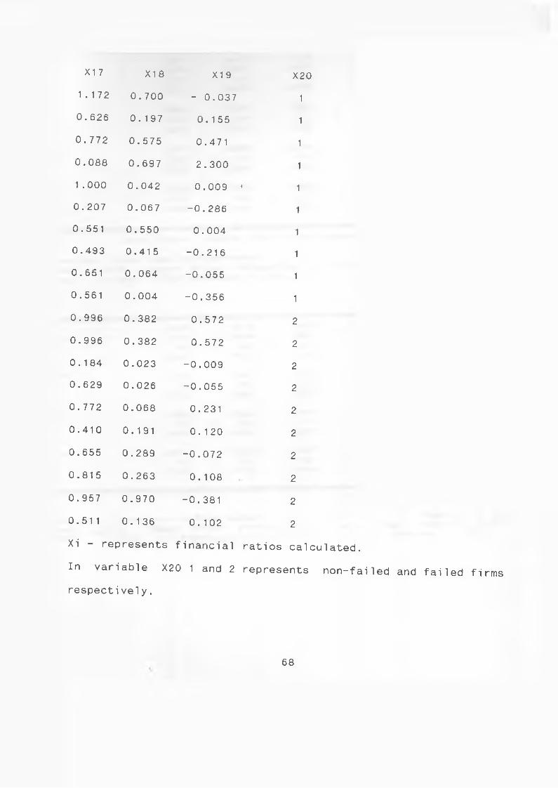
X1 7 X 1 8 X1 9 X20
1.172 0.700 - 0.037 1
0.626 0.197 0.155 1
0.772 0.575 0.471 1
0.088 0.697 2.300 1
1 .000 0.042 0.009 ' 1
0.207 0.067 -0.286 1
0.551 0.550 0.004 1
0.493 0.415 -0.216 1
0.651 0.064 -0.055 1
0.561 0.004 -0.356 1
0.996 0.382 0.572 2
0.996 0.382 0.572 2
0.184 0.023 -0.009 2
0.629 0.026 -0.055 2
0.772 0.068 0.231 2
0.410 0.191 0.120 2
0.655 0.289 -0.072 2
0.815 0.263 0.108 2
0.957 0.970 -0.381 2
0.511 0.136 0.102 2
Xi - represents financial ratios calculated.
In variable X20 1 and 2 represents non-failed and failed firms
respectively.
68
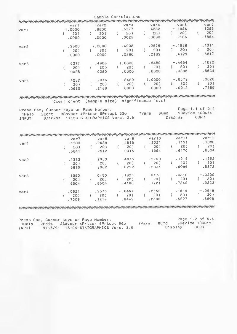
Sample Correlationsmmmmmmmmmmmmmmmmmmmmmmmmmmmmmmmmmmmmmmmmmmmmmmmmmmmhmmmmmmmmmmmmmmmmmmmmmmmmmmmm
var1 var2 var3 var4 var5 var6var1 1.0000 .9800 .6377 .4232 -.2926 .1295
( 20) ( 20) ( 20) ( 20) ( 20) ( 20).0000 .0000 .0025 .0630 .2106 . 5864
var2 .9800 1.0000 .4908 .2876 -. 1938 .1311( 20) ( 20) ( 20) ( 20) ( 20) ( 20)
.0000 .0000 .0280 .2189 .4129 .5817
var3 .6377 .4908 1.0000 .8480 -.4654 . 1070( 20) ( 20 > ( 20) ( 20) ( 20) ( 20)
.0025 .0280 .0000 .0000 .0386 .6534
var4 .4232 .2876 .8480 1.0000 -.6679 .0828( 20) ( 20) ( 20) ( 20) ( 20) ( 20)
.0630 .2189 .0000 .0000 .0013 .7285
m m m m m m m m m m m m m m m m m m m m m m m m m m m m m m m m m m m m m m m m m m m m m m m m m m m m m m m m m m m m m m m m m m m m m m m m m m m m m m m m
Coefficient (sample size) significance level
Press Esc, Cursor keys or Page Number: Page 1. 1 Of 5.41 He!p 2Edit 3Savscr •4Prtscr 5Prtopt 6Go 7Vars 8Cmd 9Device 10Quit
INPUT 9/16/91 17:59 :STATGRAPHICS Vers. 2.6 Display CORR
m m m m m m m m m m m m m m m m m m m m m m m m m m m m m m m m m m m m m m m m m m m m m m m m m m m m m m m m m m m m m m m m m m m m m m m m m m m m m m m m
var7 var8 var9 var 1 0 var1 1 varl 2var 1 . 1303 . 2638 .4818 .3021 .1191 .1080
( 20) ( 20) ( 20) ( 20) ( 20) ( 20). 5841 .2612 .0315 . 1954 .6170 .6504
var2 .1313 .2953 .4875 .2790 .1216 . 1292( 20) ( 20) ( 20) ( 20) ( 20) ( 20)
. 5810 .2062 .0292 .2336 .6096 .5872
var3 . 1080 .0450 . 1926 .3178 .0810 -.0200( 20) ( 20) ( 20) ( 20) ( 20) ( 20)
. 6504 . 8504 .4160 .1721 . 7342 .9333
var4 .0821 .3575 -.0467 .2652 .1519 -.0949( 20) ( 20) ( 20) ( 20) ( 20) ( 20)
. 7309 .1218 . 8449 . 2586 .5227 .6908
Press Esc, Cursor keys or Page Number:1Help 2Edit 3Savscr 4Prtscr 5Prtopt 6Go
INPUT 9/16/91 18:04 STATGRAPHICS Vers. 2.
Page 1.2 of 5.47Vars 8Cmd 9Device 10Quit
Display CORR
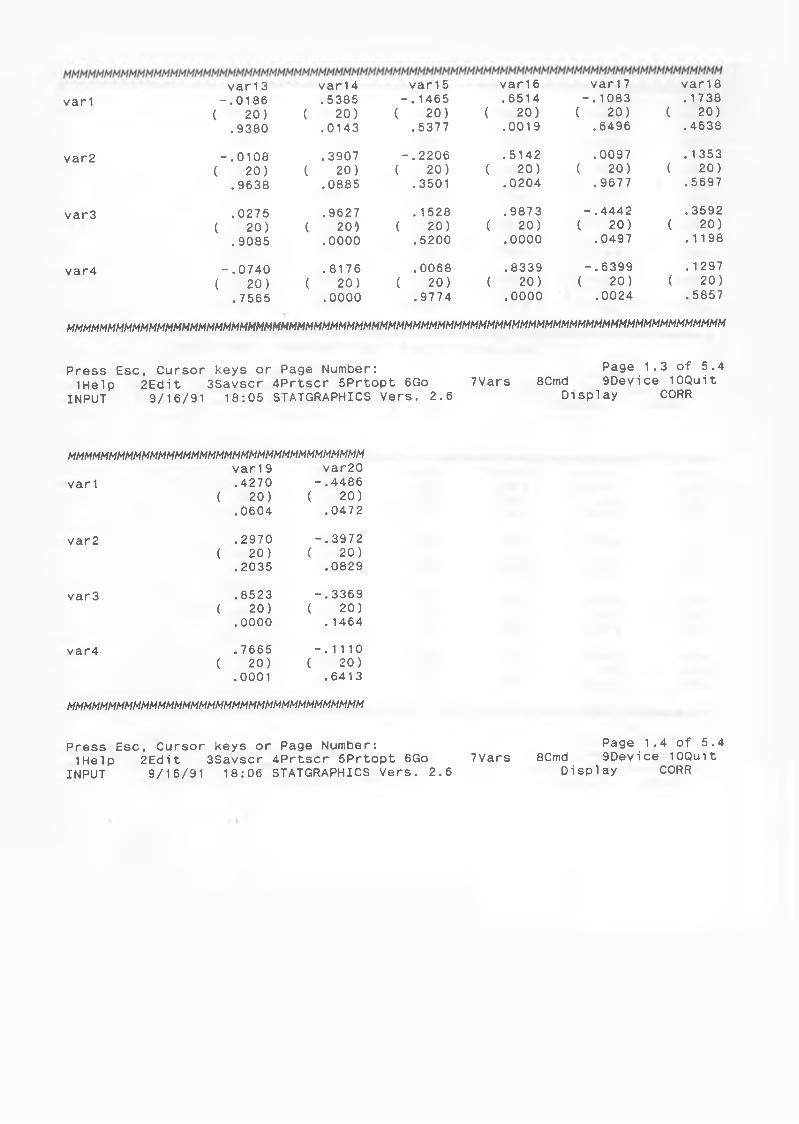
var 1 3 var14 var15 var1 6 var 1 7 var 18var 1 -.0186 .5385 -.1465 .6514 -.1083 .1738
( 20) ( 20) ( 20) ( 20) ( 20) ( 20).9380 .0143 .5377 .0019 .6496 .4638
var2 -.0108 .3907 -.2206 .5142 .0097 .1353( 20) ( 20) ( 20) ( 20) ( 20) ( 20)
.9638 .0885 .3501 .0204 .9677 .5697
var3 .0275 .9627 .1528 .9873 -.4442 .3592( 20) ( 20) ( 20) ( 20) ( 20) ( 20)
.9085 .0000 .5200 .0000 .0497 .1198
var4 -.0740 .8176 .0068 .8339 -.6399 .1297( 20) ( 20) ( 20) ( 20) ( 20) ( 20)
. 7565 .0000 .9774 .0000 .0024 .5857
mmmmmmmmmmmmmmmmmmmmmmmmmmmmmmmmmmmmmmmmmmmmmmhmmmmmmmmmmmmmmmmmmmmmmmmmmmmmmmmm
Press Esc, Cursor keys or Page Number: Page 1.3 of 5.41 Hel p 2Edit 3Savscr 4Prtscr 5Prtopt 6Go 7Vars 8Cmd 9Dev ice 10Quit
INPUT 9/16/91 18:05 !STATGRAPHICS Vers. 2.6 Display CORR
mmmmmmmmmmmmmmmmmmmmmmmmmmmmmmmmmmmmvar 1 9 var20
var 1 .4270 -.4486( 20) ( 20)
.0604 .0472
var2 .2970 -.3972( 20) ( 20)
.2035 .0829
var3 .8523 -.3369( 20) ( 20)
.0000 . 1464
var4 . 7665 -.1110( 20) ( 20)
.0001 .6413
MMMMMMMMMMMMMMMMMMMMMMMMMMMMMMMMMMMM
Press Esc, Cursor keys or Page Number: Page 1.4 of 5.41 He 1p 2Edi t 3Savscr 4Prtscr 5Prtopt 6Go
INPUT 9/16/91 18:06 STATGRAPHICS Vers. 2.67Vars 8Cmd 9Device 10Quit
Display CORR
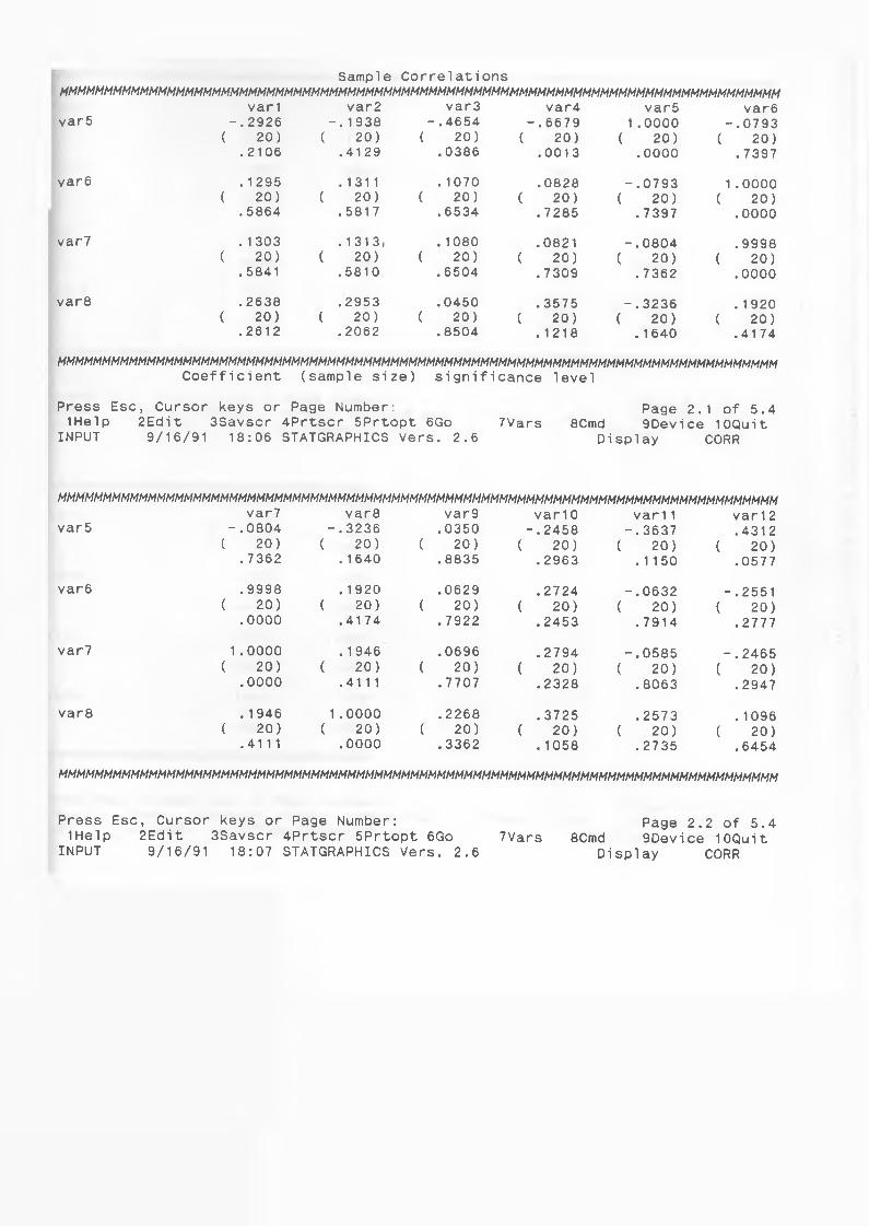
Sample Correlationsmmmmmmmmmmmmmmmmmmmmmmmmmmmmmmmmmmmmmmmmmmmmmmmmmmmmmmmmmmmmmmmmmmmmmmmmmmmmmmmm
var1 var2 var3 var4 var5 var6var5 -.2926 -. 1938 -.4654 -.6679 1.0000 -.0793
( 20) ( 20) ( 20) ( 20) ( 20) ( 20).2106 .4129 .0386 .0013 .0000 . 7397
var6 . 1295 .1311 .1070 .0828 -.0793 1.0000( 20) ( 20) ( 20) ( 20) ( 20) ( 20)
. 5864 .5817 .6534 .7285 .7397 .0000
var7 .1303 .1313, .1080 .0821 -.0804 .9998( 20) ( 20) ( 20) ( 20) ( 20) ( 20)
.5841 . 5810 .6504 .7309 . 7362 .0000
var8 .2638 .2953 .0450 .3575 -.3236 .1920( 20) ( 20) ( 20) ( 20) ( 20) ( 20)
.2612 .2062 .8504 .1218 . 1640 .4174
MMMMMMMMMMMMMMMMMMMMMMMMMMMMMMMMMMMMMMMMMMMMMMMMMMMMMMMMMMMMMMMMMMMMMMMMMMMMMMMMCoefficient (sample size) significance level
Press Esc, Cursor keys or Page Number: Page 2. 1 of 5.41Help 2Edi t 3Savscr 4Prtscr 5Prtopt 6Go 7Vars 8Cmd 9Device 10Qui t
INPUT 9/16/91 18:06 STATGRAPHICS Vers. 2.6 Display CORR
MMMMMMMMMMMMMMMMMMMMMMMMMMMMMMMMMMMMMMMMMMMMMMMMMMMMMMMMMMMMMMMMMMMMMMMMMMMMMMMMvar7 var8 var9 var10 var11 var12
var5 -.0804 -.3236 .0350 -.2458 -.3637 .4312( 20) ( 20) ( 20) ( 20) ( 20) ( 20)
.7362 . 1640 .8835 . 2963 .1150 .0577
var6 .9998 .1920 .0629 .2724 -.0632 -.2551( 20) ( 20) ( 20) ( 20) ( 20) ( 20)
.0000 .4174 .7922 .2453 .7914 .2777
var7 1.0000 .1946 .0696 .2794 -.0585 -.2465( 20) ( 20) ( 20) ( 20) ( 20) ( 20)
.0000 .4111 .7707 .2328 .8063 .2947
var8 . 1 946 1.0000 .2268 .3725 .2573 .1096( 20) ( 20) ( 20) ( 20) ( 20) ( 20)
.4111 .0000 .3362 . 1058 .2735 . 6454
MMMMMMMMMMMMMMMMMMMMMMMMMMMMMMMMMMMMMMMMMMMMMMMMMMMMMMMMMMMMMMMMMMMMMMMMMMMMMMMM
Press Esc, Cursor keys or Page Number:1Help 2Edit 3Savscr 4Prtscr 5Prtopt 6Go 7Vars
INPUT 9/16/91 18:07 STATGRAPHICS Vers. 2.6
Page 2.2 of 5.48Cmd 9Device 10Quit
Display CORR
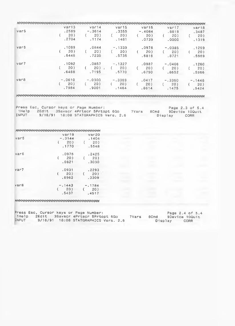
MMMMMMMMMMMMMMMMMMMMMMMMMMMMMMMMMMMMMMMMMMMMMMMMMMMMMMMMMHMMMMMMMMMMMMMMMMMMMMMM
var5var13 .2589
( 20) .2704
var 14 -.3614 ( 20)
.1174
var1 5 .3355
( 20) .1481
var16 -.4084( 20)
.0739
var1 7 .8819
( 20) .0000
var 1 8 .3487
( 20) .1319
var6 .1099 ( 20)
.6446
.0844( 20)
.7235
-.1339 ( 20)
.5735
.0978 ( 20)
.6816
-.0385 ( 20)
.8721
.1259 ( 20)
.5969
var7 . 1092 ( 20)
.6468
.0857 ( 20) ,
.7195
-.1327 ( 20)
.5770
.0987 ( 20)
.6790
-.0406 ( 20)
.8652
.1260 ( 20)
.5966
var8 -.0610 ( 20)
. 7984
-.0300 ( 20)
.9001
-.3369 ( 20)
.1464
.0417 ( 20)
.8614
-.3360 ( 20)
.1475
-.1448( 20)
.5424
MMMMMMMMMMMMMMMMMMMMMMMMMMMMMMMMMMMMMMMMMMMMMMMMMMMMMMMMMMMMMMMMMMMMMMMMMMMMMMMM
Press Esc, Cursor keys or Page Number:1Help 2Edit 3Savscr 4Prtscr 5Prtopt 6Go 7Vars
INPUT 9/16/91 18:08 STATGRAPHICS Vers. 2.6
Page 2.3 of 5.4 8Cmd 9Device 10Quit
Display CORR
MMMMMMMMMMMMMMMMMMMMMMMMMMMMMMMMMMMMvar1 9 var20
var5 -.3144 . 1404( 20) ( 20)
.1770 . 5548
var6 .0976 .2425( 20) ( 20)
.6821 .3030
var7 .0931 .2293( 20) ( 20)
.6962 .3309
var8 -. 1443 -.1784( 20) ( 20)
.5437 .4517
MMMMMMMMMMMMMMMMMMMMMMMMMMMMMMMMMMMM
Press Esc, Cursor keys or Page Number: Page 2.4 of 5.41Help 2Edit 3Savscr 4Prtscr 5Prtopt 6Go 7Vars 8Cmd 9Device 10QuitINPUT 9/16/91 18:08 STATGRAPHICS Vers. 2.6 Display CORR
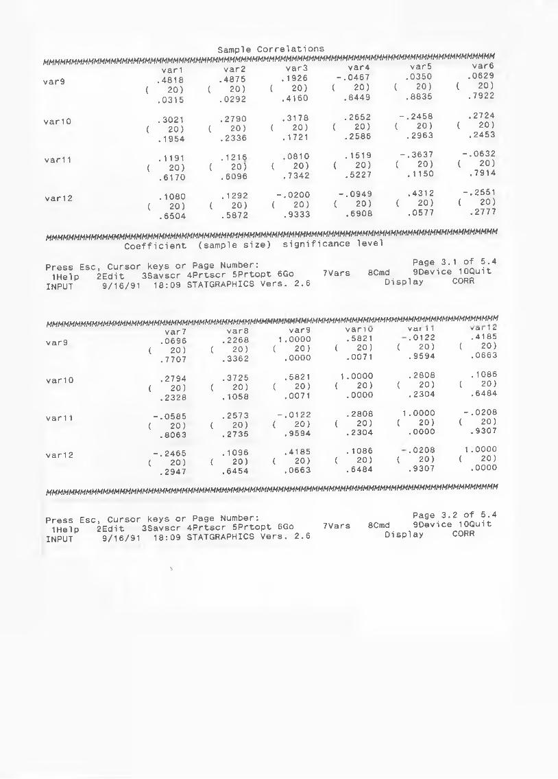
, , ^ ^ 1 »/ar<3 var3 var4 var5 var6
Sample Correlationsmmmmmmmmmmmmmmmmmmmmmmmmmmmmmmmmmmmmmmmmmmmmmmmmmmmmmmmmmmmmmmmmmmmmmmmmmmmmmmmm
var9var 1 .4818
( 20) .0315
var2 .4875
( 20) .0292
var3 .1926
( 20) .4160
var4 -.0467 ( 20)
.8449
var5 .0350
( 20) .8835
var6 .0629
( 20) .7922
var10 .3021 ( 20)
.1954
.2790 ( 20)
.2336
.3178 ( 20)
.1721
.2652 ( 20)
.2586
-.2458 ( 20)
.2963
.2724 ( 20)
.2453
var 11 .1191 ( 20)
.6170
.1216 ( 20)
. 6096
.0810 ( 20)
.7342
.1519 ( 20)
.5227
-.3637 ( 20)
.1150
-.0632 ( 20)
.7914
var 1 2 .1080 ( 20)
.6504
.1292 ( 20)
.5872
-.0200 ( 20)
.9333
-.0949 ( 20)
.6908
.4312 ( 20)
.0577
-.2551 ( 20)
.2777
mmmhmmmmmmmmmmmmmmmmmmmmmmmmmmmmmmmmmmmmmmmmmmmmmmmmmmmmmmmmmmmmmmmmmmmmmmmmmmmm
Coefficient (sample size) significance level
Press Esc, Cursor keys or Page Number:1Help 2Edit 3Savscr 4Prtscr 5Prtopt 6Go 7Vars
INPUT 9/16/91 18:09 STATGRAPHICS Vers. 2.6
Page 3.1 of 5.4 8Cmd 9Device 10Quit
Display CORR
mmmmmmmmmmmmmmmmmmmmmmmmmmmmmmmmmmmmmmmmmmmmmmmmmmmmmmmmmmmmmmmmmmmmmmmmmmmmmmmm
var7var9 .0696
( 20 ) .7707
var10 .2794( 20 )
.2328
var11 - •0585( 20)
.8063
var12 -.2465( 20)
.2947
var8 var9 V.2268 1.0000 .
( 20) ( 20) (.3362 .0000 •
.3725 .5821 1 .( 20) ( 20) (
.1058 .0071 •
.2573 -.0122 .( 20) ( 20) (
.2735 .9594 •
. 1096 .4185 .( 20) ( 20) (
. 6454 .0663 •
ar l u 5821 20)
0071(
var i i .0122 20)
. 9594
V Cl 1 1 c..4185
( 20) .0663
000020)
0000(
. 2808 20)
.2304
.1086 ( 20)
.6484
280820)
2304
1(
.000020)
.0000
-.0208 ( 20)
.9307
108620)
6484(
.020820)
.9307
1.0000 ( 20)
.0000
mmmmmmmmmmmmmmmmmmmmmmmmmmmmmmmmmmmmmmmmmmmmmmmhmmmmmmmmmmmmmmmmmmmmmmmmmmmmmmmm
Press Esc, Cursor keys or Page Number:1Help 2Edit 3Savscr 4Prtscr 5Prtopt 6Go 7Vars
INPUT 9/16/91 18:09 STATGRAPHICS Vers. 2.6
Page 3.2 of 5.48Cmd 9Device 10Quit
Display CORR
V
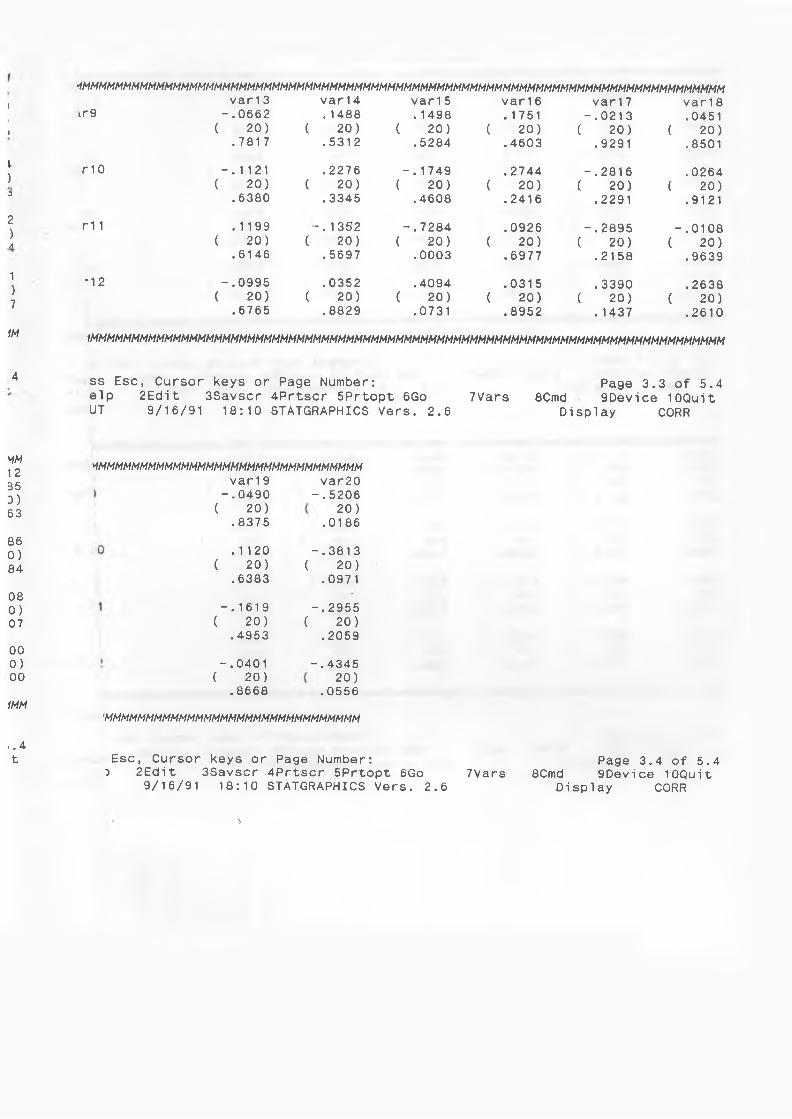
'1MMMMMMMMMMMMMMMMMMMMMMMMMMMMMMMMMMMMMMMMMMMMMMMMMMMMMMMMMMMMMMMMMMMMMMMMMMMMMM1 var 1 3 var 14 var1 5 var1 6 var 1 7 var 1 81 ir9 -.0662 .1488 .1498 .1751 -.0213 .0451) ( 20) ( 20) ( 20) ( 20) ( 20) ( 20)
.7817 .5312 .5284 .4603 .9291 .8501V)
r 10 -.1121 .2276 -.1749 .2744 -.2816 .0264( 20) ( 20) ( 20) ( 20) ( 20) ( 20)J .6380 .3345 .4608 .2416 .2291 .9121
2
)Ar11 .1199 -.13S2 -.7284 .0926 -.2895 -.0108
( 20) ( 20) ( 20) ( 20) ( 20) ( 20).6146 . 5697 .0003 .6977 .2158 . 9639
1)7
-12 -.0995 .0352 .4094 .0315 .3390 .2638( 20) ( 20) ( 20) ( 20) ( 20) ( 20)1 .6765 .8829 .0731 .8952 . 1437 .2610
1M 1MMMMMMMMMMMMMMMMMMMMMMMMMMMMMMMMMMMMMMMMMMMMMMMMMMMMMMMMMMMMMMMMMMMMMMMMMMMMM
4 ss ESC, Cursor keys or Page Number: Page 3.,3 Of 5.4elp 2Edit 3Savscr 4Prtscr 5Prtopt 6Go UT 9/16/91 18:10 STATGRAPHICS Vers. 2.6
7Vars 8Cmd 9Device 10Quit Display CORR
MM12350)63
860)84
080)07
000)00
1MM
MMMMMMMMMMMMMMMMMMMMMMMMMMMMMMMMMvar 1 9
-.0490 ( 2 0 )
.8375
.1120 ( 20 )
.6383
-.1619 ( 20 )
.4953
-.0401 ( 20)
.8668
var20 -.5206
20) .0186
-.3813 ( 2 0 )
.0971
-.2955 ( 20)
.2059
-.43452 0 )
.0556
'MMMMMMMMMMMMMMMMMMMMMMMMMMMMMMMi .4 t Esc, Cursor keys or Page Number:
3 2Edit 3Savscr 4Prtscr 5Prtopt 6Go9/16/91 18:10 STATGRAPHICS Vers. 2.6
Page 3.4 of 5.47Vars 8Cmd 9Device 10Quit
Display CORR
v
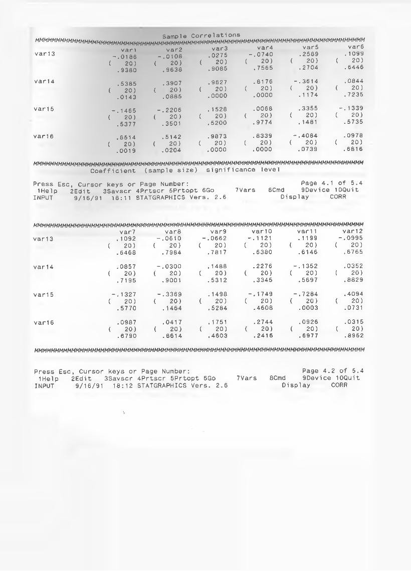
uar3 var4 var5 var6
Sample Correlationsmmmmmmmmmmmmmmmmmmmmmmmmmmmmmmmmmmmmmmmmmmmmmmmmmmmmmmmmmmmmmmmmmmmmmmmmmmmmmmmm
v a n var2 var3 var4 var5 var6var 13 -.0186 -.0108 .0275 -.0740 .2589 . 1099
( 20) ( 20) ( .9638
20) ( 20) ( 20) ( 20). 9380 .9085 . 7565 .2704 . 6446
var14 .5385 .3907 .9627 .8176 -.3614 .0844( 20)
.0143( 20) ( 20) ( 2 0 ) ( 20) ( 20)
.0885 .0000 .0000 .1174 .7235
var1 5 -. 1465 -.2206 .1528 .0068 .3355 -.1339( 20) ( 20) ( 20) ( 2 0 ) ( 20) ( 20)
.5377 .3501 .5200 .9774 . 1481 .5735
var1 6 .6514 .5142 .9873 .8339 -.4084 .0978( 20) ( 2 0 ) ( 20) ( 2 0 ) ( 20) ( 20)
.0019 .0204 .0000 .0000 .0739 .6816
MMMMMMMMMMMMMMMMMMMMMMMMMMMMMMMMMMMMMMMMMMMMMMMMMMMMMMMMMMMMMMMMMMMMMMMMMMMMMMMH
Press Esc 1 Hel p
Coefficient (sample size) significance level
, Cursor keys or Page Number:2Edit 3Savscr 4Prtscr 5Prtopt 6Go 7Vars 8Cmd
Page 4.1 9Device
of 5.4 1OQui t
INPUT 9/16/91 18:11 STATGRAPHICS Vers . 2.6 Display CORR
HMMMMMMMMMMMMMMMMMMMMMMMMMMMMMMMMMMMMMHMMMMMMMMMMMMMMMMMMMMMMMMMMMMMMMMMMMMMMMMMvar7 var8 var9 var10 var11 var1 2
var1 3 . 1092 -.0610 -.0662 -.1121 .1199 -.0995( 20) ( 20) ( 20) ( 20) ( 20) ( 20)
.6468 . 7984 . 7817 .6380 .6146 . 6765
var14 .0857 -.0300 .1488 .2276 -.1352 .0352( 20) ( 20) ( 20) ( 20) ( 20) ( 20)
.7195 .9001 .5312 .3345 .5697 .8829
var 1 5 -.1327 -.3369 .1498 -.1749 -.7284 .4094( 20) ( 20) ( 20) ( 20) ( 20) ( 20)
.5770 .1464 .5284 .4608 .0003 .0731
var1 6 .0987 .0417 .1751 .2744 .0926 .0315( 20) ( 20) ( 20) ( 20) ( 20) ( 20)
.6790 .8614 .4603 .2416 .6977 .8952
MMMMMMMMMMMMMMMMMMMMMMMMMMMMMMMMMMMMMMMMMMMMMMMMMMMMMMMMMMMMMMMMMMMMMMMMMMMMMMMM
Press Esc, Cursor keys or Page Number:1Help 2Edit 3Savscr 4Prtscr 5Prtopt 6Go 7Vars
INPUT 9/16/91 18:12 STATGRAPHICS Vers. 2.6
Page 4.2 of 5.48Cmd 9Device 10Quit
Display CORR
*
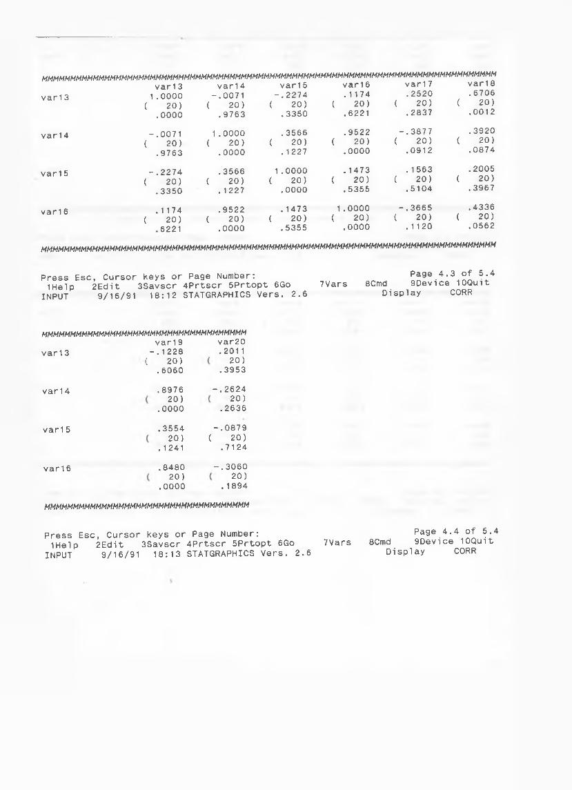
mmmmmmmmmmmmmmmmmmmmmmmmmmmmmmmmmmmmmmmmmmmmmmmmmmmmmmmmmmmmmmmmmmmmmmmmmmmmmmmm
var 1 3var 1 3 1.0000
( 20) .0000
var 14 -.0071 ( 20)
.9763
var1 5 -.2274 ( 20)
.3350
var 1 6 .1174
( 20) .6221
var 1 7 .2520
( 20) .2837
var 18 .6706
( 20) .0012
var 14 -.0071 ( 20)
.9763
1.0000 ( 20)
.0000
.3566 ( 20)
.1227
.9522 ( 20)
.0000
-.3877 ( 20)
.0912
.3920 ( 20)
.0874
var15 -.2274 ( 20)
.3350
.3566 ( 20)
.1227
1.0000 ( 20)
.0000
.1473 ( 20)
.5355
.1563 ( 20)
.5104
.2005 ( 20)
.3967
var1 6 .1174( 20)
.6221
.9522 ( 20)
.0000
.1473( 20)
.5355
1.0000 ( 20)
.0000
-.3665 ( 20)
.1120
.4336 ( 20)
.0562
mmmmmmmmmmmmmmmmmmmmmmmmmmmmmmmmmmmmmmmmmmmmmmmmmmmmmmmmmmmmmmmmmmmmmmmmmmmmmmmm
Press Esc, Cursor keys or Page Number:1Help 2Edit 3Savscr 4Prtscr 5Prtopt 6Go 7Vars
INPUT 9/16/91 18:12 STATGRAPHICS Vers. 2.6
Page 4.3 of 5.4 8Cmd 9Device 10Quit
Display CORR
mmmmmmmmmmmmmmmmmmhmmmmmmmmmmmmmmmmm
var1 3var1 9
-. 1228 : 20 )
.6060
var20.2011
2 0 )
.3953
var14 .89762 0 )
.0000
-.26242 0 )
.2636
var1 5 .355420 )
.1241(-.0879
20 ).7124
var 16 .84802 0 )
.0000
-.306020 )
.1894
MMMMMMMMMMMMMMMMMMMMMMMMMMMMMMMMMMMM
Press Esc, Cursor keys or Page Number:1Help 2Edit 3Savscr 4Prtscr 5Prtopt 6Go
INPUT 9/16/91 18:13 STATGRAPHICS Vers. 2.67Vars 8Cmd
Page 4.4 9Devi ce
of 5.4 10Qui t
Display CORR
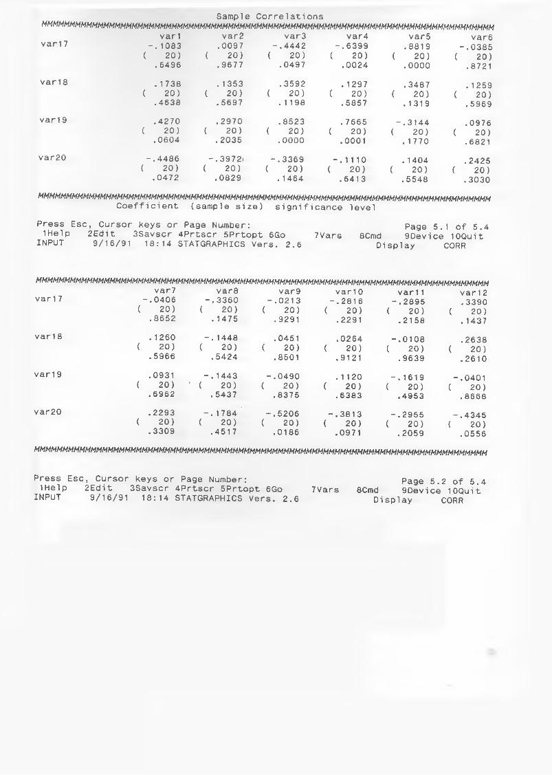
Sample Correlationsmmmmmmmmmmmmmmmmmmmmmmmmmmmmmmmmmmmmmmmmmmmmmmmmmmmmmmmmmmmmmmmmmmmmmmmmmmmmmmmm
var 1 7van var2 var3 var4 var5 var6
-.1083 .0097 -.4442 -.6399 .8819 -.0385( 20) ( 20) ( 20) ( 20) ( 20) ( 20)
. 6496 .9677 .0497 .0024 .0000 .8721
var 18 . 1 738 . 1353 .3592 .1297 .3487 . 1259( 20) ( 20) ( 20) ( 20) ( 20) ( 20)
.4638 .5697 .1198 .5857 .1319 .5969
var1 9 .4270 .2970 .8523 . 7665 _ .3144 .0976( 20) ( 20) ( 20) ( 20) ( 20) ( 20)
.0604 . 2035 .0000 .0001 . 1770 .6821
var20 -.4486 ~.3972i -.3369 -.1110 . 1404 .2425( 20) ( 20) ( 20) ( 20) ( 20) ( 20)
.0472 .0829 . 1464 .6413 .5548 .3030
mmmmmmmmmmmmmmmmmmmmmmmmmmmmmmmmmmmmmmmmmmmmmmmmmmmmmmmmmmmmmmmmmmmmmmmmmmmmmmmmCoefficient (samp 1e size) significance level
Press Esc, Cursor keys or Page Number: Page 5. 1 of 5.41Help 2Edit 3Savscr 4Prtscr 5Prtopt 6 Go 7Vars 8Cmd 9Device 10QuitINPUT 9/16/91 18:14 STATGRAPHICS Vers. 2.6 Display CORR
mmmmmmmmmmmmmmmmmmmmmmmmmmmmmmmmmmmmmmmmmmmmmmmmmmmmmmmmmmmmmmmmmmmmmmmmmmmmmmmmvar7 var8 var9 var10 var11 var12
var17 -.0406 -.3360 -.0213 -.2816 -.2895 .3390( 20) ( 20) ( 20) ( 20) ( 20) ( 20)
.8652 .1475 .9291 .2291 .2158 .1437
var 1 8 . 1260 ( 20)
.5966
-. 1448 ( 20)
. 5424
.0451 ( 20)
.8501
.0264 ( 20)
.9121
-.0108( 20)
.9639
.2638 ( 20)
.2610varl 9 .0931
( 20) ‘ .6962
-.1443 ( 20)
. 5437
-.0490 ( 20)
.8375
.1120 ( 20)
.6383
-.1619 ( 20)
.4953
-.0401 ( 20)
.8668var20 .2293
( 20) .3309
-.1784 ( 20)
.4517
-.5206 ( 20)
.0186
-.3813 ( 20)
.0971
-.2955 ( 20)
.2059
-.4345 ( 20)
.0556
mmmmmmmmmmmmmmmmmmmmmmmmmmmmmmmmmmmmmmmmmmmmmmmmmmmmmmmmmmmmmmmmmmmmmmmmmmmmmmmm
Press Esc 1Help
INPUT
, Cursor 2Ed i t 9/16/91
keys or Page Number:3Savscr 4Prtscr 5Prtopt 6Go
18:14 STATGRAPHICS Vers. 2.67Vars
Page 5.2 of 5.48Cmd 9Device 10Quit
Display CORR
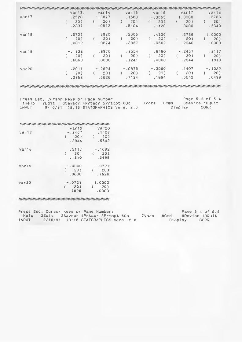
MMMMMMMMMMMMMMMMMMMMMMMMMMMMMMMMMMMMMMMMMMMMMMMMMMMMMMMMMMMMMMMMMMMMMMMMMMMMMMMMvar13. var 14 var1 5 var 16 var 17 var18
var 1 7 .2520 -.3877 .1563 -.3665 1.0000 .2788( 20) ( 20) ( 20) ( 20) ( 20) ( 20)
.2837 .0912 .5104 .1120 .0000 .2340
var 18 .6706 .3920 .2005 .4336 .2788 1.0000( 20) ( 20) ( 20) ( 20) ( 20) ( 20)
.0012 .0874 .3967 .0562 .2340 .0000
var 19 -.1228 .8976 .3554 .8480 -.2467 .3117( 20) ( 20) ( 20) ( 20) ( 20) ( 20)
.6060 .0000 .1241 .0000 . 2944 .1810
var20 .201 1 -.2624 -.0879 -.3060 . 1407 -.1082( 20) ( 20) ( 20) ( 20) ( 20) ( 20)
.3953 .2636 .7124 .1894 .5542 .6499
MMMMMMMMMMMMMMMMMMMMMMMMMMMMMMMMMMMMMMMMMMMMMMMMMMMMMMMMMMMMMMMMMMMMMMMMMMMMMMMM
Press Esc, Cursor keys or Page Number: Page 5.3 of 5.41Help 2Edit 3Savscr 4Prtscr 5Prtopt 6Go 7Vars 8Cmd 9Device 10Quit
INPUT 9/16/91 18:15 STATGRAPHICS Vers. 2.6 Display CORR
MMMMMMMMMMMMMMMMMMMMMMMMMMMMMMMMMMMMvar 1 9 var20
var 1 7 -.2467 .1407( 20) ( 20 )
.2944 .5542
var 18 .3117 - . 1082( 20) ( 20)
.1810 .6499
var 1 9 1.0000 - .0721( 20) ( 20)
.0000 . 7626
var20 -.0721 1. 0000( 20) ( 20)
. 7626 . 0000
Press Esc, Cursor keys or Page Number: Page 5.4 of 5.41Help 2Edit 3Savscr 4Prtscr 5Prtopt 6Go 7Vars 8Cmd 9Device 10Quit
INPUT 9/16/91 18:15 STATGRAPHICS Vers. 2.6 Display CORR


