P u b l i s h i n g

Editor-in-ChiefDr M Flannigan, Canadian Forest Service, Edmonton, Canada.

IJWF is published for the International Association of Wildland Fire by:

CSIRO PUBLISHINGPO Box 1139 (150 Oxford Street)Collingwood, Victoria 3066Australia

Telephone:+61 3 9662 7644 (editorial enquiries)+61 3 9662 7668 (subscription enquiries and claims)

Fax: +61 3 9662 7611 (editorial enquiries)+61 3 9662 7555 (subscription enquiries and claims)

Email: publishing.ijwf@csiro.au (editorial enquiries)publishing.sales@csiro.au (subscription enquiries and claims)

Please submit all new manuscripts directly to CSIRO PUBLISHING, inelectronic form only. See the IJWF Notice to Authors for more information.

w w w . p u b l i s h . c s i r o . a u / j o u r n a l s / i j w f

Volume 11, 2002© International Association of Wildland Fire 2002

International Journalof Wildland Fire

Scientific Journal of IAWF

© IAWF 2002 10.1071/WF02003 1049-8001/02/030183

International Journal of Wildland Fire, 2002, 11, 183–191

WF02003Oklahoma Fir e Danger M odelJ. D. Car lsonet al .

The Oklahoma Fire Danger Model: An operational tool for mesoscale fire danger rating in Oklahoma

J. D. CarlsonA, Robert E. BurganB, David M. EngleC and Justin R. GreenfieldD

A Biosystems and Agricultural Engineering, Oklahoma State University, 214 Ag Hall, Stillwater, OK 74078, USA.

Corresponding author: Telephone: +1 405 744 6353; fax: +1 405 744 6059; email: jdc@okstate.edu B USDA Forest Service, Fire Sciences Laboratory, Rocky Mountain Research Station,

Missoula, MT 59807, USA. (retired)C Plant and Soil Sciences, Oklahoma State University, Stillwater, OK 74078, USA.

D Oklahoma Climatological Survey, University of Oklahoma, Norman, OK 73019, USA.

This paper is derived from a presentation at the 4th Fire and Forest Meteorology Conference, Reno, NV, USA, held 13–15 November 2001

Abstract. This paper describes the Oklahoma Fire Danger Model, an operational fire danger rating system for thestate of Oklahoma (USA) developed through joint efforts of Oklahoma State University, the University ofOklahoma, and the Fire Sciences Laboratory of the USDA Forest Service in Missoula, Montana. The model is anadaptation of the National Fire Danger Rating System (NFDRS) to Oklahoma, but more importantly, represents thefirst time anywhere that NFDRS has been implemented operationally using hourly weather data from a spatiallydense automated weather station network (the Oklahoma Mesonet). Weekly AVHRR satellite imagery is alsoutilized for live fuel moisture and fuel load calculations. The result is a near-real-time mesoscale fire danger ratingsystem to 1-km resolution whose output is readily available on the World Wide Web(http://agweather.mesonet.ou.edu/models/fire). Examples of output from 25 February 1998 are presented.

The Oklahoma Fire Danger Model, in conjunction with other fire-related operational tools, has proven useful tothe wildland fire management community in Oklahoma, for both wildfire anticipation and suppression and forprescribed fire activities. Instead of once-per-day NFDRS information at two to three sites, the fire manager nowhas statewide fire danger information available at 1-km resolution at up to hourly intervals, enabling a quickerresponse to changing fire weather conditions across the entire state.

Additional keywords: fire danger; model; automated weather station networks; Oklahoma Mesonet; remotesensing; fuels; fuel moisture; National Fire Danger Rating System.

Introduction

With more than half of its 17.5 million ha consisting ofwildlands, the importance of fire in Oklahoma (USA), bothnatural and prescribed, is apparent. During a typical yearabout 450 000 ha of Oklahoma land is burned: 364 000 ha byprescribed fire and another 86 000 ha by wildfire. During thesevere 1995–1996 fire season, over 263 000 ha of Oklahomaland was burned by wildfire alone.

With a view toward user-friendly dissemination ofweather-based tools for wildland fire management inOklahoma, Oklahoma State University (OSU) and theUniversity of Oklahoma (OU) have been cooperating overthe past 6 years in developing various fire-relatedoperational tools for dissemination over the World Wide

Web. In place of hourly synoptic-scale weather information,15-min mesoscale weather information is now available fromover 110 Oklahoma sites and, in place of once-per-day firedanger information at two to three sites, statewide colorizedfire danger maps are available at 1-km resolution at up tohourly intervals.

The most important factor behind the development ofthese weather-based, fire-related management tools has beenthe Oklahoma Mesonet, the state’s automated weathermonitoring station network which became operational in1994 (Brock et al. 1995). A joint project of OSU and OU, thenetwork currently consists of 115 stations having an averagespacing of 30 km. Weather and soil observations aretransmitted every 15 min, with the data being available onthe Web typically within 30 min after being reported.

184 J. D. Carlson et al.

Another major factor has been the cooperation betweenOSU, OU, and the Fire Sciences Laboratory of the USDAForest Service in Missoula, Montana. This collaboration,which began in late 1993, resulted in the development of theOklahoma Fire Danger Model, which was implemented in itsoriginal form on the World Wide Web in March 1996. Thisparticular timing was motivated by an extreme fire season inOklahoma which began in the fall of 1995 and lasted throughthe spring of 1996; in particular, a 2-day statewide wildfireemergency during 22–23 February 1996 provided even moreimpetus for making the model accessible.

The Oklahoma Fire Danger Model

The Oklahoma Fire Danger Model (OKFD) is an adaptationof the USDA Forest Service’s National Fire Danger RatingSystem (Deeming et al. 1977; Bradshaw et al. 1983; Burgan1988) to Oklahoma but implemented, for the first timeanywhere, to 1-km resolution using hourly weather data froma spatially dense automated weather station network(Carlson and Engle 1998). Weekly satellite imagery for livefuel moisture and fuel load calculations are also utilized,which also represents a departure from past applications ofNFDRS. Currently the OKFD model is run 11 times eachday (0000, 0500, 0700, 0900, 1100, 1300, 1400, 1500, 1600,1700, 1900 local standard time), with greater frequency(hourly) during the afternoon times of peak fire danger.Output is available at the following World Wide Webaddress generally within 1 h of the valid run time(http://agweather.mesonet.ou.edu/models/fire).

Model output (examples to be shown later) include color-coded maps to 1-km resolution of the following NationalFire Danger Rating System (NFDRS) components: burningindex, spread component, energy release component, andignition component. In addition, interpolated maps of 1-hdead fuel moisture and the Keetch-Byram drought index(KBDI) are available, the latter map being updated oncedaily. A table of these and other fuel/weather variables ateach automated weather monitoring station site used in themodel is also provided.

In addition to the model output, the Web site featuresweekly color-coded maps of visual and relative greenness(Burgan and Hartford 1993), examples of model outputfrom wildfire episode days, and KBDI comparisons of eachmonth in the current year to the corresponding month 1 yearago.

OKFD model components

To obtain the best assessment of fire danger at any scalerequires information about the three components of thefire environment: weather, fuels, and topography. Thefirst component of this ‘fire environment triangle’ is themost dynamic and the one used in all operational firedanger systems, whereas the third one is the leastdynamic.

Weather

Although not all weather monitoring stations are automated,automated weather monitoring stations are now the norm andtheir number continues to increase. Such stations provide thecapability to assess fire danger more than once daily ifappropriate revisions in the fire danger model being used canbe made to take advantage of the increased weather dataflow.

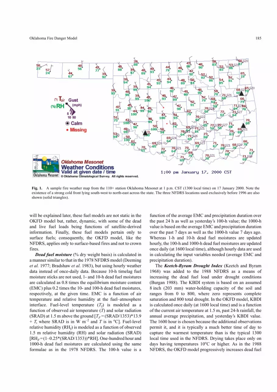
An outstanding example of such an automated weatherstation network is the Oklahoma Mesonet (Carlson et al.1994; Elliott et al. 1994), consisting currently of 115 stationsand reporting data every 15 min. It is from this network thatthe Oklahoma Fire Danger Model gets its weatherinformation. An example of a typical fire weather map thatis available from the Oklahoma Mesonet is shown in Fig. 1.One can easily locate the position of a strong cold front onthis afternoon, with strong south-west winds ahead (east) ofthe front and lighter north-west winds behind it. For ourOklahoma clientele, temperatures are shown in degreesFahrenheit (oF), relative humidity in %, and wind speed inmiles per hour (mph). Note that such a map is updated every15 min, allowing for near-real-time monitoring of fireweather conditions.

With respect to the OKFD Model itself, the weathervariables utilized include 1.5-m air temperature and relativehumidity, 10-m wind speed, solar radiation, andprecipitation. Before the implementation of this model in1996, NFDRS computations in Oklahoma were performedusing once-a-day weather data from only two or threelocations: two automated sites (one in south-west Oklahomaand one in eastern Oklahoma) and periodically from onemanual site in north-east Oklahoma (McDowell, personalcommunication). These three site locations aresuperimposed upon Fig. 1 and depicted by solid triangles.The resulting map shows the obvious superiority of theOklahoma Mesonet with respect to spatial density. Temporalsuperiority over once-a-day data is provided by using hourlydata (although the fire weather maps themselves are updatedevery 15 min). In the present NFDRS application, hourlydata are utilized from 115 stations of the OklahomaMesonet.

Fuels

Fuel models from the 1988 NFDRS are utilized to representOklahoma’s land surface. With the aid of 1-km resolutionAVHRR satellite imagery (Loveland et al. 1991), a fuels mapfor Oklahoma was developed for us by the Fire SciencesLaboratory in Missoula in consultation with other firescientists in Oklahoma. The result is that each squarekilometer pixel in Oklahoma has been assigned one of fiveNFDRS fuel models: Model P for pine forests; Model R fordeciduous forests; Model T for tallgrass prairie andeastern/central cropland; Model L for mixed prairie andwestern cropland; and Model A for shortgrass prairie. As

Oklahoma Fire Danger Model 185

will be explained later, these fuel models are not static in theOKFD model but, rather, dynamic, with some of the deadand live fuel loads being functions of satellite-derivedinformation. Finally, these fuel models pertain only tosurface fuels; consequently, the OKFD model, like theNFDRS, applies only to surface-based fires and not to crownfires.

Dead fuel moisture (% dry weight basis) is calculated ina manner similar to that in the 1978 NFDRS model (Deeminget al. 1977; Bradshaw et al. 1983), but using hourly weatherdata instead of once-daily data. Because 10-h timelag fuelmoisture sticks are not used, 1- and 10-h dead fuel moisturesare calculated as 0.8 times the equilibrium moisture content(EMC) plus 0.2 times the 10- and 100-h dead fuel moistures,respectively, at the given time. EMC is a function of airtemperature and relative humidity at the fuel–atmosphereinterface. Fuel-level temperature (Tf) is modeled as afunction of observed air temperature (T) and solar radiation(SRAD) at 1.5 m above the ground [TF = (SRAD/1353)*13.9+ T, where SRAD is in W m–2 and T is in oC]. Fuel-levelrelative humidity (RHf) is modeled as a function of observed1.5 m relative humidity (RH) and solar radiation (SRAD)[RHF = (1–0.25*(SRAD/1353))*RH]. One-hundred hour and1000-h dead fuel moistures are calculated using the sameformulae as in the 1978 NFDRS. The 100-h value is a

function of the average EMC and precipitation duration overthe past 24 h as well as yesterday’s 100-h value; the 1000-hvalue is based on the average EMC and precipitation durationover the past 7 days as well as the 1000-h value 7 days ago.Whereas 1-h and 10-h dead fuel moistures are updatedhourly, the 100-h and 1000-h dead fuel moistures are updatedonce daily (at 1600 local time), although hourly data are usedin calculating the input variables needed (average EMC andprecipitation duration).

The Keetch-Byram Drought Index (Keetch and Byram1968) was added to the 1988 NFDRS as a means ofincreasing the dead fuel load under drought conditions(Burgan 1988). The KBDI system is based on an assumed8 inch (203 mm) water-holding capacity of the soil andranges from 0 to 800, where zero represents completesaturation and 800 total drought. In the OKFD model, KBDIis calculated once daily (at 1600 local time) and is a functionof the current air temperature at 1.5 m, past 24-h rainfall, theannual average precipitation, and yesterday’s KBDI value.The 1600 hour is chosen because the additional observationspermit it, and it is typically a much better time of day tocapture the warmest temperature than is the typical 1300local time used in the NFDRS. Drying takes place only ondays having temperatures 10oC or higher. As in the 1988NFDRS, the OKFD model progressively increases dead fuel

Fig. 1. A sample fire weather map from the 110+ station Oklahoma Mesonet at 1 p.m. CST (1300 local time) on 17 January 2000. Note theexistence of a strong cold front lying south-west to north-east across the state. The three NFDRS locations used exclusively before 1996 are alsoshown (solid triangles).

186 J. D. Carlson et al.

loads (from a ‘drought’ dead fuel load reservoir) as KBDIvalues in a given 1-km pixel rise above 100 (Burgan 1988).

In addition to using an automated weather stationnetwork, the OKFD model also relies on weekly satelliteimagery for estimation of live fuel moisture. Thisrepresents another aspect in which the OKFD model differsfrom former applications of NFRDS. Since the early 1990s,biweekly and (in recent years) weekly composites ofAVHRR-derived NDVI (Normalized Difference VegetationIndex) to 1-km resolution (Holben 1986; Goward et al.1990) have been used in the USA to assess the status of livevegetation through derived variables called ‘visualgreenness’ and ‘relative greenness’ (Burgan and Hartford1993; Burgan et al. 1996). Both variables can range from 0to 100%, but the latter is based on the historical maximumand minimum NDVI values for a given 1-km pixel. Thesethree variables have proven useful in monitoring ‘greenup’and senescence as well as showing departures in a givenweek from what is ‘normal’. The OKFD model utilizes onlyrelative greenness (RG) derived for each 1-km pixel fromNDVI data obtained through weekly composites of AVHRRdata and each pixel’s NDVI historical maximum andminimum values. The relative greenness values are thenemployed to estimate live fuel moisture (% dry weightbasis) for both herbaceous and woody fuel components.Live herbaceous moisture (%) is calculated as 2*RG + 29(if this yields a value less than 30%, the live fuel moisture isset to the 1-h dead fuel moisture value). Live woodymoisture (%) is calculated as 1.5*RG + 50 + 10*CLIM,where CLIM is the NFDRS ‘climate class’ (1, 2, or 3 inOklahoma).

In the OKFD model the fuel loadings for both live and1-h dead fuels are dynamic. The herbaceous fuel load variesin direct proportion to the weekly RG value[(RG/100)*(fuel model herb load)], while the part notconsidered live [(1–RG/100)*(fuel model herb load)] isadded to the fuel model’s specified 1-h dead fuel load. Thewoody fuel load in pixels with deciduous understories (fuelmodels R and P) is also a function of the weekly RG value,with woody fuel load being set to [(RG/100)*(fuel modelwoody load)] and the remaining ‘non-live’ portion[(1–RG/100)*(fuel model woody load)] being transferred tothe 1-h dead fuel load. Finally, it has already been noted thatthe dead fuel loads in all timelag categories are alsofunctions of KBDI, with increasing proportional amounts ofdead fuel added from the fuel model’s ‘drought’ load asKBDI values rise above 100.

Topography

With respect to topography, all slopes calculated inOklahoma to 1-km resolution from a GIS system yieldedvalues within NFDRS slope class 1 (i.e. slopes from 0 to25%). Thus, each square kilometer pixel in the model has

slopes assumed to be in the 0–25% range. For locally greaterslopes, the model cannot be relied upon for accurate output.

OKFD model methodology

As with any model involving near-real-time data, theproblem of missing data comes into play. Missing stationdata in the hourly Mesonet data files are estimated byobjective analysis using a Barnes interpolation scheme(Barnes 1964) with a cutoff radius of 130 km. Weights areexponentially damped by the square of the distance. Thisinterpolation occurs before the model calculations areperformed, ensuring observed or interpolated values at eachof the Mesonet sites.

The OKFD model consists of two major parts. The firstpart, using hourly station data since the last OKFD run,calculates the four timelag dead fuel moistures and KBDIvalues (as well as some other needed weather-relatedvariables) at the 110+ Mesonet sites. These variables are theninterpolated via the Barnes scheme to a 10-km squareresolution rectangular grid covering Oklahoma. Thisparticular resolution is chosen because it lies at the lowerlimit of recommended grid spacing for an average Mesonetstation spacing of 30 km (Koch et al. 1983). Decreasing thegrid size further would be computationally more intensivewhile gaining nothing in terms of accuracy.

The second part of the OKFD model utilizes the 10-kmgridded output in combination with already available 1-kmpixel data to calculate the live fuel moistures and NFDRSfire danger indices on a 1-km pixel scale. Certainvariables, such as the fuel model and relative greennessvalue, are already available on a pixel basis. Othervariables for the pixel calculations (e.g. precipitation, windspeed, dead fuel moistures, KBDI) are obtained viabilinear interpolation to the pixel in question using thefour nearest grid point values from the 10-km grid square.The objective analysis grid was chosen such that all pixelswithin Oklahoma fall within the external boundaries of thegrid (i.e. every pixel has four surrounding grid points fromwhich to interpolate). If the pixel contains a Mesonet site,the actual calculated data for that site from the first part ofthe model is utilized, however, rather than interpolateddata. Even though no station data from other states areused, interpolation results near state boundaries are stillwithin the range of acceptability, given the high spatialdensity (30 km) of the Oklahoma Mesonet.

Examples of OKFD model output

In this section we present examples of OKFD model outputfrom 25 February 1998. Even though no unusual wildfireactivity was reported on this day, the maps to be shown serveas excellent examples of the capability of the OKFD modelin assessing fire danger in the mesoscale range. Figure 2shows the Mesonet fire weather map from 2 p.m. CentralStandard Time (1400 local time). Note the existence of a ‘dry

Oklahoma Fire Danger Model 187

line’ (depicted by the superimposed dashed line), which is adiscontinuity in relative humidity. Behind the dry line (to thewest) much lower relative humidities exist (in the 10–40%range); ahead of the dry line (to the east), relative humiditiesin the 60–90% range are common. Also note the change inwind direction from south and south-east ahead of the dryline (bringing up moisture from the Gulf of Mexico) tosouth-westerly behind it (bringing in much drier air fromwestern Texas and New Mexico). Wind speeds are alsohigher behind the dry line, with gusts in the 30–40 miles perhour range (13–18 m s–1). The three NFDRS locations usedexclusively before 1996 are again shown for purposes ofcomparison (solid triangles).

The corresponding 1-h dead fuel moisture map calculatedby the OKFD model is shown in Fig. 3. Note the strongdiscontinuity in moisture values (reds to greens) occurringalong and just ahead of the dry line. Much lower fine-fuelmoistures (3–8% range) exist west of the dry line, with muchhigher values (15–25% range) to the east. [The two localizedregions of lower 1-h dead fuel moisture near the easternborder of Oklahoma are reflective of the lower relativehumidities reported by the Mesonet sites in these areas(Fig. 2) as well as the local gradients in relative humidityutilized by the objective analysis scheme.]

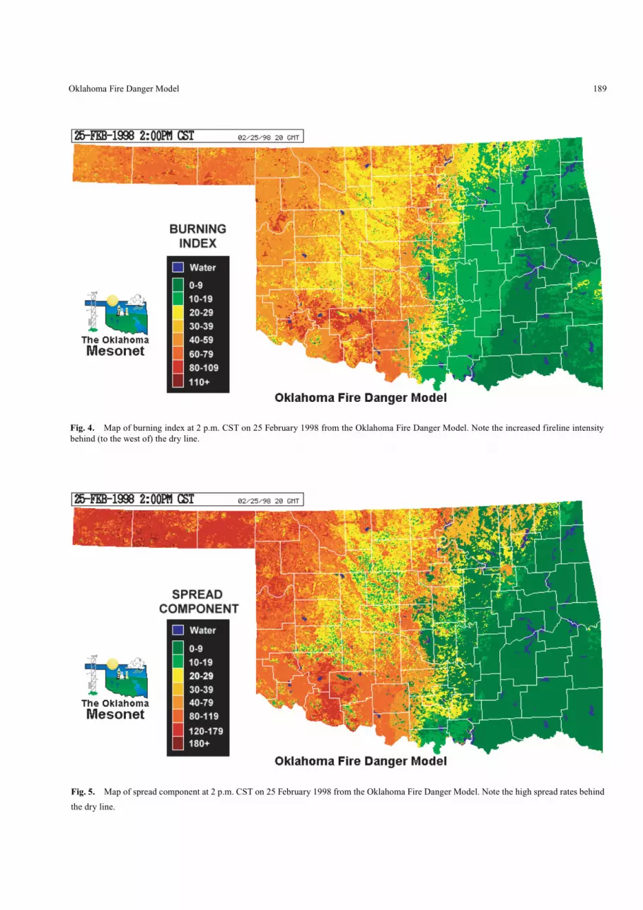
Figure 4 depicts the burning index across Oklahoma at thesame time. Burning index (BI) is directly related to firelineintensity and is perhaps the most useful fire danger indexfrom the NFDRS. It is scaled numerically such that the BIvalue divided by 10 equals the flame length (in feet) of theheadfire. Note the increased fire danger to the west of the dryline (BI values in the 25–95 range); these values correspondto flame lengths of 0.8–2.9 m. To the east of the dry line, firedanger is much lower, with BI values in the 10–19 rangeimmediately east of the line and even lower values (0–9)further east.

Finally, Fig. 5 depicts the corresponding spreadcomponent map. The spread component (SC) is a measure ofhow fast the headfire is moving and is numerically equal tothe rate of spread in feet per minute. Again, note the strongdiscontinuity along the dry line. With the exception of thewinter wheat belts, which are green this time of year andwhose mitigating effects on fire danger are easily seen in thismap as well as in the BI map (the yellow and green areas westof the dry line), spread component values in the 40–130category are common (spread rates of 0.2–0.7 m s–1) to thewest of the dry line; at one of the Mesonet stations in thepanhandle, an SC value as high as 177 was calculated(0.90 m s–1 spread rate). To the east of the dry line, spreadrates are dramatically lower, with most of south-eastOklahoma in the 0–9 range.

Through these examples one can easily see theimportance of a mesoscale automated weather stationnetwork to fire danger assessment. The Mesonet stationspacing density of 30 km allows one to see the exact

locations of features such as dry lines and cold fronts, whilethe near-real-time availability of data (every 15 min in thecase of the fire weather maps) allows one to follow theprogress of such features across the area of concern.

Most of Oklahoma’s fires involve only 1-h and 10-h fuels,which respond rapidly to changing weather conditions andfeatures such as dry lines. Under the ‘old’ system of threeonce-a-day NFDRS sites, the exact location of the dry line inthe example above along with its corresponding effects onfire danger would have been entirely missed, as would itsmovement over time (speed and direction). According to thefire chief of Oklahoma Forestry Services (a frequent user ofthe Oklahoma Mesonet and the OKFD model), firefightersin Oklahoma are interested in the fire danger indices nearestthe location of the fire (not just at several sites, which maybe far from the actual fire) and nearest the time of the fire,not at 1300 yesterday or earlier today (McDowell, personalcommunication). The Oklahoma Mesonet and the OKFDmodel have the capability of capturing the volatility ofOklahoma weather and its effects on fire danger, which canvary dramatically over space and time.

Use of the OKFD model and other fire weather products

In addition to the Oklahoma Fire Danger Model, otheroperational tools for wildland fire management have beendeveloped in conjunction with programming support at OU(Carlson et al. 1998; Carlson 2001). These include: (1) Current and recent fire weather maps (going back 6 h in

15-min increments) and maps of recent rainfall over thepast 1, 3, 6, 12, 24, 48, and 72 h (http://agweather.-mesonet.ou.edu/current-recent-weather);

(2) The Oklahoma Dispersion Model (Carlson and Arndt1998), a tool for use in smoke management (http://ag-weather.mesonet.ou.edu/models/dispersion); and

(3) 60-h MOS (Multiple Output Statistics) forecasts fromthe Nested Grid Model (http://agweather.mesonet.ou.-edu/forecasts).

Depending upon the product, the output is updated in timescales ranging from 15 min (in the case of Mesonet fireweather, rainfall, and dispersion maps) to as much as 12 h (inthe case of the NGM MOS forecasts). All of these productscan be accessed via the Oklahoma Mesonet AgWeatherhome page (http://agweather.mesonet.ou.edu).

Since their inception, all the fire-related management toolshave been popular products, used by a wide range of clientelein Oklahoma. Although recent statistics are not available, thenumber of Web page ‘hits’ through 12 June 2001 were asfollows: Oklahoma Fire Danger Model (40 151 hits since2 June 1997); NGM MOS forecasts (20 238 hits since 28 July1997); and the Oklahoma Dispersion Model (3767 hits since1 May 1998). Oklahoma Forestry Services consults theseproducts, particularly the Oklahoma Fire Danger Model, ona regular basis to aid in wildfire preparedness levels andin issuance of Red Flag Fire Alerts and burning ban

188 J. D. Carlson et al.

Fig. 2. Fire weather map from 2 p.m. CST (1400 local time) on 25 February 1998. Note the existence of a dry line oriented roughly north tosouth across central Oklahoma (depicted by the superimposed dashed line). The three NFDRS locations used exclusively before 1996 are againdepicted (solid triangles).

Fig. 3. Map of 1-h dead fuel moisture at 2 p.m. CST on 25 February 1998 from the Oklahoma Fire Danger Model. Note the correspondingdiscontinuity in fuel moisture along and just ahead (to the east) of the dry line.

Oklahoma Fire Danger Model 189

Fig. 5. Map of spread component at 2 p.m. CST on 25 February 1998 from the Oklahoma Fire Danger Model. Note the high spread rates behind

the dry line.

Fig. 4. Map of burning index at 2 p.m. CST on 25 February 1998 from the Oklahoma Fire Danger Model. Note the increased fireline intensitybehind (to the west of) the dry line.

190 J. D. Carlson et al.

recommendations to the Governor. State emergencymanagers and local fire chiefs also utilize these operationaltools to monitor fire danger. Finally, the fire managementproducts provide guidance for prescribed burning activitiesand are used by federal and state agencies as well as byprivate and public landowners involved in this arena.

Summary

This paper has focused on the Oklahoma Fire Danger Model(OKFD), an operational mesoscale fire danger rating systemfor Oklahoma. A joint project of Oklahoma State University,the University of Oklahoma, and the Fire SciencesLaboratory of the USDA Forest Service in Missoula,Montana, the model is an adaptation of the National FireDanger Rating System (NFDRS) to Oklahoma but, for thefirst time anywhere, using a spatially dense automatedweather station network (the Oklahoma Mesonet) of 110+stations for hourly weather data. Weekly AVHRR satelliteimagery is also used for live fuel moisture and fuel loadcalculations, in contrast to earlier applications of NFDRS.Model output consists of colorized maps to 1-km resolutionof four NFDRS components, as well as interpolated maps of1-h dead fuel moisture and Keetch-Byram drought index. TheOKFD model is currently run 11 times per day, with outputavailable at http://agweather.mesonet.ou.edu/models/fire.

In conjunction with fire weather maps updated every15 min, the OKFD model constitutes a vast improvementover the situation in Oklahoma prior to 1996. Before then,only two to three weather stations were used in NFDRS firedanger calculations, and those calculations were based ononce-per-day observations. This contrasts with the currentsituation, in which rapid access (via the World Wide Web) to1-km resolution fire danger maps at time intervals as smallas 1 h allows fire managers to visually analyse the effects ofOklahoma’s changing weather over space and time. Becausemost of Oklahoma’s fires involve only 1- and 10-h fuels,which respond rapidly to changing weather conditions, thecurrent system allows fire managers to adjust theirdispatching and safety procedures accordingly as conditionsimprove or deteriorate. Oklahoma fire managers now haveaccess to fire danger information close to the location of thefire (not just at several sites, which may be far from theactual fire) and close to the time of the fire (not at 1300 theday before or earlier in the current day).

In addition to the OKFD model, other products ofrelevance to fire management have been developed. Theseinclude current/recent fire weather maps (a 6-h archive isavailable) and rainfall maps (amounts over the past 1, 3, 6,12, 24, 48, and 72 h); the Oklahoma Dispersion Model; and60-h NGM MOS forecasts. These products have also provenuseful to the wildland fire management community, both interms of wildfire anticipation and suppression and forprescribed fire activities.

Future work with respect to the Oklahoma Fire DangerModel will include incorporating numerical weather forecastmodel output into the OKFD model to predict future firedanger conditions across Oklahoma. In addition, we plan toreplace the 1-, 10-, 100-, and 1000-h dead fuel moisturealgorithms with numerical models developed by Nelson(Carlson et al. 1996; Nelson 2000). Finally, we look to futuredevelopments in the remote sensing of live fuels to help usimprove both our mapping and selection of fuel models aswell as our estimation of live fuel moistures and loads.

Acknowledgements

The authors would like to thank a number of people withoutwhom the Oklahoma Fire Danger Model and its associatedproducts would not be possible. First, we are grateful to LarryBradshaw and Bobbie Bartlette of the Fire SciencesLaboratory in Missoula for helping in the development andremote sensing aspects of the Oklahoma Fire Danger Model.We also thank those fire scientists in Oklahoma who helpedus determine appropriate fuel models for the state: they includeTerry Bidwell (OSU), Ron Masters (at the time, OSU), andMark Moseley (USDA-NRCS). We are indebted to those atthe Oklahoma Climatological Survey at OU who implementedthe various fire-related products on Mesonet computerplatforms; aside from the fourth author of this paper whoimplemented the OKFD model, we wish to thank Derek Arndt,who was responsible for implementing the other fire-relatedproducts. Finally, we thank Pat McDowell, fire chief ofOklahoma Forestry Services, for his constructive commentson our fire products and for his regular usage of them.

References

Barnes S (1964) A technique for maximizing details in numericalweather map analysis. Journal of Applied Meteorology 3,396–409.

Bradshaw LS, Deeming JE, Burgan RE, Cohen JD (1983) ‘The 1978National Fire-Danger Rating System: technical documentation’.USDA Forest Service, Intermountain Forest and Range ExperimentStation General Technical Report INT–169. 44 pp.

Brock FV, Crawford KC, Elliott RE, Cuperus GW, Stadler SJ, JohnsonHL, Eilts MD (1995) The Oklahoma Mesonet: a technicaloverview. Journal of Atmospheric and Oceanic Technology 12,5–19.

Burgan RE (1988) ‘1988 revisions to the 1978 National Fire-DangerRating System’. USDA Forest Service, Southeastern ForestExperiment Station Research Paper SE–273. 39 pp.

Burgan RE, Hartford RA (1993) ‘Monitoring vegetation greenness withsatellite data’. USDA Forest Service, Intermountain ResearchStation General Technical Report INT–297. 13 pp.

Burgan RE, Hartford RA, Eidenshink JC (1996) ‘Using NDVI to assessdeparture from average greenness and its relation to fire business’.USDA Forest Service, Intermountain Research Station GeneralTechnical Report INT-GTR–333. 8 pp.

Carlson JD (2001) Operational wildland fire management systems: theOklahoma example. Preprints, Fourth Symposium on Fire andForest Meteorology, American Meteorological Society, 13–15November 2001, Reno, NV, pp. 140–147.

Oklahoma Fire Danger Model 191

http://www.publish.csiro.au/journals/ijwf

Carlson JD, Arndt DS (1998) The Oklahoma Dispersion Model: a Web-based management tool for agricultural practices associated withnear-surface releases of gases and particulates. Preprints, 23rdConference on Agricultural and Forest Meteorology, AmericanMeteorological Society, 2–7 November 1998, Albuquerque, NM,pp. 337–340.

Carlson JD, Engle DM (1998) Recent developments in the OklahomaFire Danger Model, a mesoscale fire danger rating system forOklahoma. Preprints, Second Symposium on Fire and ForestMeteorology, American Meteorological Society, 11–16 January1998, Phoenix, AZ, pp. 42–47.

Carlson JD, Engle DM, Shafer MA (1994) Using the OklahomaMesonet as a fire management tool. Proceedings, 12th Conferenceon Fire and Forest Meteorology, Society of American Foresters,26–28 October 1993, Jekyll Island, GA, pp. 31–37.

Carlson JD, Engle DM, Greenfield JR, Arndt DS (1998) Developmentand dissemination of near-real-time, weather-based tools for firemanagement in Oklahoma. Preprints, Second Symposium on Fireand Forest Meteorology, American Meteorological Society, 11–16January 1998, Phoenix, AZ, pp. 48–51.

Carlson JD, Nelson RM Jr., Engle DM (1996) Field measurementof dead fuel moisture for model development andimplementation on the Oklahoma Mesonet. Preprints, 22ndConference on Agricultural and Forest Meteorology with

Symposium on Fire and Forest Meteorology, AmericanMeteorological Society, 28 January–2 February 1996, Atlanta,GA, pp. 276–279.

Deeming JD, Burgan RE, Cohen JD (1977) ‘The national fire-dangerrating system–1978’. USDA Forest Service, Intermountain Forestand Range Experiment Station General Technical Report INT–39.63 pp.

Elliott RL, Brock FV, Stone ML, Harp SL (1994) Configurationdecisions for an automated weather station network. AppliedEngineering in Agriculture 10, 45–51.

Keetch JJ, Byram GM (1968) ‘A drought index for forest fire control’.USDA Forest Service, Southeastern Forest Experiment StationResearch Paper SE–38. 32 pp.

Koch SE, DesJardins M, Kocin PJ (1983) An interactive Barnes objectivemap analysis scheme for use with satellite and conventional data.Journal of Climate and Applied Meteorology 22, 1487–1503.

Loveland TR, Merchant JW, Ohlen DO, Brown JF (1991) Developmentof a land-cover characteristics database for the conterminous U.S.Photogrammetric Engineering and Remote Sensing 57, 1453–1463.

McDowell P, personal communication (2002) Forestry Services,Oklahoma Department of Agriculture.

Nelson RM Jr. (2000) Prediction of diurnal change in 10-h fuel stickmoisture content. Canadian Journal of Forest Research 30,1071–1087.