The Effects of Building Representation and Clustering in Large-Eddy Simulations of Flows in Urban Canopies

Boundary-Layer Meteorol (2009) 132:415–436DOI 10.1007/s10546-009-9410-6

ARTICLE

The Effects of Building Representation and Clusteringin Large-Eddy Simulations of Flows in Urban Canopies

Elie Bou-Zeid · Jan Overney · Benedict D. Rogers ·Marc B. Parlange

Received: 24 November 2008 / Accepted: 7 July 2009 / Published online: 23 July 2009© Springer Science+Business Media B.V. 2009

Abstract We perform large-eddy simulations of neutral atmospheric boundary-layer flowover a cluster of buildings surrounded by relatively flat terrain. The first investigated questionis the effect of the level of building detail that can be included in the numerical model, a topicnot yet addressed by any previous study. The simplest representation is found to give similarresults to more refined representations for the mean flow, but not for turbulence. The winddirection on the other hand is found to be important for both mean and turbulent parameters.As many suburban areas are characterised by the clustering of buildings and homes into smallareas separated by surfaces of lower roughness, we look at the adjustment of the atmosphericsurface layer as it flows from the smoother terrain to the built-up area. This transition hasunexpected impacts on the flow; mainly, a zone of global backscatter (energy transfer fromthe turbulent eddies to the mean flow) is found at the upstream edge of the built-up area.

Keywords Building representation · Global backscatter · Heterogeneous terrain ·Surface roughness · Turbulent kinetic energy · Urban boundary layer · Urban canopy

1 Introduction

The combination of changing climate patterns and increasing urban populations willintensify the pressure on the infrastructure and the environment in urban zones and

E. Bou-Zeid (B)Department of Civil and Environmental Engineering, Princeton University,C326-EQuad, Princeton, NJ 08544, USAe-mail: [email protected]

E. Bou-Zeid · J. Overney · M. B. ParlangeSchool of Architecture, Civil and Environmental Engineering,École Polytechnique Fédérale de Lausanne-EPFL, Lausanne, Switzerland

B. D. RogersSchool of Mechanical, Aerospace and Civil Engineering, University of Manchester,P.O. Box 88, Sackville Street Building, Sackville Street, Manchester M60 1QD, UK

123

416 E. Bou-Zeid et al.

will continue to give rise to a complex set of problems concerning the health, safety, andcomfort of urban populations.

Urban areas represent an important environment due to the high population density, thestrong concentration of economic activity, and the associated land-use modification. There-fore, to address and mitigate the aforementioned problems, an improved understanding ofthe dynamics of this urban environment, and of its interaction with the surrounding naturalsystems, is required. Of particular interest are the dynamics of atmospheric flows in built-upareas and their impact on air quality, energy consumption, and urban microclimates. Researchefforts concentrating on urban atmospheric dynamics are nevertheless lagging behind ourneeds and more efforts are required, especially in relation to the understanding of local atmo-spheric dynamics over cities and the development of adequate parameterisations for urbanareas in large-scale numerical models (Britter and Hanna 2003; Coceal and Belcher 2004).

The basic challenge is related to the heterogeneity and complexity of urban environmentscombined with a lack of experimental and numerical tools appropriate for sensing and mod-elling the complex dynamics of urban systems, especially atmospheric flow and transport inurban canopies and flow-structure interactions (Rotach et al. 2002; Cheng and Castro 2002;Xie and Castro 2006). On the one hand, transport issues concerning pollutants, heat, andmoisture are strongly coupled to the fluid dynamics within and over the urban canopy. Onthe other hand, flow patterns in these regions are strongly modified by the presence of thebuildings and of the anthropogenic heat sources.

A related problem also concerns the lack of adequate parameterisations for the interactionof urban areas with their surroundings at larger scales. When weather and global circulationmodels are used, even large cities only cover the lowest part of one or a few grid cells. Insuch instances, the physical processes that occur within the building canopies cannot be sim-ulated explicitly and must be parameterised. Development of good parameterisations at thecity/regional scale is interconnected with improving our understanding of the neighbourhood-scale and street-scale atmospheric dynamics in urban areas.

In the past two decades, experimental urban canopy studies have been conducted quiteextensively with the primary objective of improving the basic understanding of flow andtransport in urban environments (Grimmond et al. 1998; Emeis 2004b; Emeis and Turk 2004;Eliasson et al. 2006; Roth et al. 2006) and with the long term aim of improving regional-scale parameterisations of urban surfaces in regional atmospheric models (Grimmond andOke 1999; Emeis 2004a; Roulet et al. 2005; Coceal and Belcher 2004). Most of theseparameterisations rely on a modified form of the Monin-Obukhov Similarity Theory (MOST,Monin and Obukhov 1954) to compute average vertical fluxes of momentum, heat, and otherscalars (see review in Rotach et al. 2002). MOST is strictly applicable only over homoge-neous surfaces, although it has often been used successfully to compute aggregate fluxes overheterogeneous natural terrains (Parlange and Brutsaert 1993; Avissar 1995; Brutsaert 1998;Molod et al. 2003; Bou-Zeid et al. 2004). Nevertheless, its universal applicability to aggregatefluxes over complex urban heterogeneities has been questioned by reviews of observationaldata (Roth 2000).

Recent studies have proposed more elaborate urban canopy parameterisations by incor-porating explicit models for building drag rather than using an average surface roughness(Belcher et al. 2003 ). Some parameterisations also include models for the energy budgetin the urban canopies (Masson 2000; Dupont and Mestayer 2006; also see comparison offour models in Roberts et al. 2006) including many realistic effects such as shadowing andradiation trapping induced by the street canyons (e.g. Harman and Belcher 2006).

However, at present it is difficult to assess these parameterisations against realistic datasince experimental studies cannot provide complete spatial information and are limited to one

123

The Effects of Building Representation and Clustering in Large-Eddy Simulations 417

site, or at most a few specific sites. This limitation makes measurements of aggregate fluxes,which represent the primary product or output of urban boundary-layer parameterisations,very challenging.

In that regard, the development of accurate numerical techniques to study urban canopyflow is valuable since such techniques provide more complete datasets describing the tur-bulent urban wind and scalar fields, as well as aggregate fluxes at the city scale. Numericalstudies can give complete spatial information and examine a very wide variety of geometriesand scenarios. This in turn implies that the physics behind specific flow features and the roleof coherent structures and the pressure field can be better studied.

The main challenge for numerical simulations of turbulent flows is the need to parame-terize the unresolved physical processes and scales, and then rigorously validate the model.The large-eddy simulation (LES) technique now offers great potential since it minimizes theneed for unresolved physics parameterization and hence usually compares better with exper-imental or field data than the traditional Reynolds-averaged numerical simulations (RANS),where all the scales of turbulence are parameterised (see examples of LES versus RANScomparison in Xie and Castro 2006 and Tominaga et al. 2008). The technique also has beenwidely used and validated in recent years for natural (Albertson et al. 2001; Lin and Glen-dening 2002; Bou-Zeid et al. 2005; Kumar et al. 2006; Kleissl et al. 2006) and urban (Cai1999; Kanda et al. 2004; Calhoun et al. 2005; Xie and Li 2005; Zhang et al. 2006; Tsenget al. 2006) boundary layers.

This paper uses the code validated in Bou-Zeid et al. (2005) and Kumar et al. (2006)for flat terrain, in Yue et al. (2007a, b) for flow in porous corn canopies, and in Tseng et al.(2006) for built-up areas (see details in Sect. 2) to address an important issue concerning theuse of the LES technique for urban environments: how much of the building details need tobe included in the modelling domain. To the best of our knowledge, this is the first study ofurban-canopy simulations sensitivity to building representation. Subsequently, we examinethe effect of discontinuities in the built environment on the flow: except for the centres ofmedium and large cities, most built environments consist of clusters of building and housesseparated by areas with other land-use types (typically with lower roughness). Nevertheless,the effects of transitions from flat/vegetated to built-up terrain, and vice versa, have not yetbeen adequately addressed.

In Sect. 2, the LES formulation and the numerical details of the numerical code aredescribed. Section 3 presents four simulations with different wind directions and differentlevels of detail in the representation of the buildings in the numerical domain. In Sect. 4, wecompute the average drag exerted by the cluster of buildings on the flow and the effectivesurface roughness of the buildings, exploring along the way the effect of wind direction andthe level of detail in building representation on the results. Section 5 depicts the effect of thebuildings on mean and turbulent velocity fields, and in Sect. 6, the adjustment of the incom-ing flow over the simulated building canopy is explored. The effect of the buildings on theshear production and dissipation of turbulent kinetic energy in the atmosphere is presentedin Sect. 7.

The simulated area is the campus of the École Polytechnique Fédérale de Lausanne (EPFL)in Switzerland. The site was selected since it is currently the location of a series of field cam-paigns to test the use of distributed sensing networks (and new-generation remote sens-ing systems) in complex urban environments. Ultimately, the aim of the research effort isto develop new approaches and frameworks for combining sensing and modelling tools inurban areas. This paper however deals strictly with the computational modelling part. Thecampus is more representative of suburban areas with discontinuous clusters of low buildingsthan of extended large city centres with many high rise towers.

123


2 Numerical Simulations

The large-eddy simulation technique has emerged as a tool of choice for high Reynoldsnumber turbulent flows in engineering systems (Piomelli 1999; Sagaut 2003), oceans (Shenand Yue 2001; Keylock et al. 2005), rivers (Bradbrook et al. 2000), and the atmosphere(Albertson and Parlange 1999a, b; Wood 2000; Bou-Zeid et al. 2004, 2007; Stoll and Porte-Agel 2006).

In the atmosphere, turbulence is mostly present in the atmospheric boundary layer (ABL),where turbulent motions span several orders of magnitude and turbulence is mainly generatedby wind shear and buoyancy. The scale of the smallest turbulent motions, the Kolmogorovscale, is on the order of 10−3 m, while the largest scales are of the size of the boundary-layer depth (≈500–2,000 m). The density of the computational grid required to capture thesescales of turbulence is currently far beyond the capacities of even the largest computationalefforts (see a discussion of computational costs of turbulent simulations in Celani 2007). Bysplitting the turbulent structures into resolved and subgrid-scale, using a filtering operation,LES reduces the density of the computational grid required to capture the large scales of theflow, making unsteady, three-dimensional simulations of high Reynolds number turbulentflows over large domains practicable.

The underlying assumption justifying this approach is that the largest eddies contain mostof the energy and are responsible for most of the transport of momentum and scalars. None-theless, the effect of the subgrid-scale structures cannot be discarded and appears in thefiltered Navier–Stokes equations as the divergence of an additional unknown, the subgrid-scale (SGS) stress tensor.

The isothermal LES equations in rotational form are solved here to ensure conservationof mass and kinetic energy of the inertial term (Orszag and Pao 1974),

∂ ui

∂xi= 0, (1a)

∂ ui

∂t+ u j

(∂ ui

∂x j− ∂ u j

∂xi

)= − 1

ρ

∂ p∗

∂xi− ∂τi j

∂x j+ Fi , (1b)

where the tilde (∼) denotes the resolved part of the variables, ui is the fluid velocity indirection i , Fi is the mean streamwise pressure forcing, ρ is the fluid density, and τi j is thedeviatoric or anisotropic part of the SGS stress tensor σi j ,

τi j = σi j − 1

3σkkδi j . (2)

We solve the equations pre-normalised with the domain-averaged friction velocity at thesurface (u∗), the boundary-layer depth (H ), and air density (ρ) so that resultant fields arealready normalised with these parameters. Of specific importance for the subsequent analysisis the fact that the simulated velocity profiles are normalised with u∗. The forcing term withthis normalization becomes Fi = �P H/ρu2∗Lx = 1, where �P is the mean streamwisepressure forcing and Lx is the streamwise length of the domain; this represents the balancebetween mean pressure forcing and surface drag at the bottom of the domain. Note that in thefiltered Navier–Stokes equations, the molecular viscous term is neglected because the focusis on very high Reynolds number flows where viscosity is negligible at the resolved scales(its effect is relevant only at much smaller scales) and the wall layer is modelled (as opposedto resolving the viscous sublayer, see Pope 2000). The isotopic or hydrostatic part of the SGSstress tensor acts as a pressure and is therefore combined with the modified pressure term

123


p∗ = p + (1/3)ρσkk + (1/2)ρu j u j . (3)

The pressure is computed from a Poisson equation obtained by setting the divergence of themomentum equation to zero. This is equivalent to (and hence substitutes for) solving thecontinuity equation.

To close the system of equations, a parameterization for the subgrid-scale stress is required.The results of large-eddy simulations are quite sensitive to this parameterization especially inthe vicinity of solid boundaries where the subgrid-scale fluxes are important and their physicsare harder to model (see the discussion in Meneveau and Katz 2000, and an illustration inBou-Zeid et al. 2005).

Most SGS parameterisations used in LES rely on the concept of eddy viscosity, νT , torelate the SGS stress (its deviatoric part) to the resolved rate of strain. The classic eddy-viscosity model proposed by Smagorinsky (1963) also uses the mixing-length concept toestimate eddy viscosity according to

τsmagi j = −2νT Si j = −2(cs�)2|S|Si j , (4)

where � is the grid scale and Si j = 0.5(∂ ui/∂x j + ∂ u j/∂xi

)is the resolved strain rate ten-

sor. The Smagorinsky coefficient, cs , is the only unknown and extensive research has beenperformed to determine its value. Lilly (1967) was the first to derive the value of cs underhomogeneous and isotropic flow conditions; subsequently, several procedures to computethe coefficient dynamically, from information about the smallest resolved scales, have beenproposed starting with Germano et al. (1991). This has allowed the application of the model torealistic flows (very rarely homogeneous and isotropic), and in many ways has represented amassive advance in the field of computational fluid dynamics. Herein, we use a more refinedmodel that takes into account the scale dependence of the model coefficients, which wasignored in Germano et al. (1991). The details of the development and formulation of thisLagrangian (Meneveau et al. 1996) scale-dependent (Porte-Agel et al. 2000; Bou-Zeid et al.2008) dynamic SGS model and the numerical details of the code can be found in Bou-Zeidet al. (2005). In addition to the validation for urban flows presented below, the model hasbeen thoroughly validated for ABL flows over homogeneous and heterogeneous surfaces(Bou-Zeid et al. 2004, 2005), diurnal ABL cycles (Kumar et al. 2006; Kleissl et al. 2006),and flow in plant canopies (Yue et al. 2007a, b).

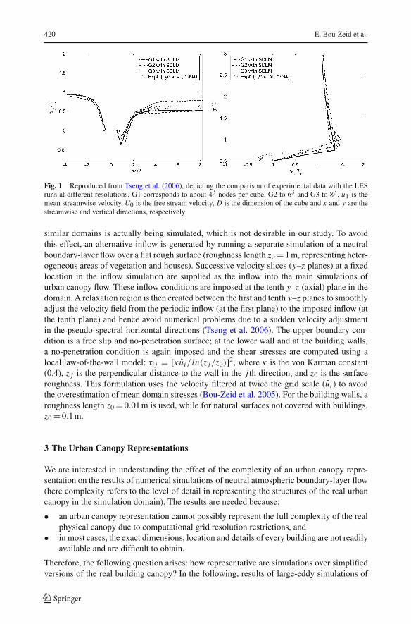
The presence of buildings is simulated using the immersed boundary method (IBM) thatmimics the effect of the buildings by imposing a virtual body force at each grid node insidethe bluff body, such that the flow velocity within the bluff body is reduced to zero. Shearstresses are imposed at the building surfaces using a regular wall-model. Tseng et al. (2006)detail the IBM implementation for the model used here and validate it against wind-tunneldata for flow over a single cube (Lyn and Rodi 1994) and an array of cubes (Meinders andHanjalic 1999, 2002). Detailed grid resolution and sensitivity studies were also conductedby Tseng et al. (2006) who concluded that beyond a grid resolution of about 63 nodes percube, results converged and a good match with experimental data was obtained. At a reso-lution of about 43 nodes per cube, the match with experimental results was not as good, butwas still representative of the basic flow dynamics, as depicted in Fig. 1 below, reproducedfrom Tseng et al. (2006) (note that the resolution requirements differ between codes thatresolve the viscous sublayer and codes that use wall models, as we do here). Hence, we basethe analysis of our results on these guidelines with a resolution of 43 nodes per cube beingconsidered adequate only for a qualitative description of the flow.

The code is pseudo-spectral in the horizontal directions, requiring periodic horizontalboundary conditions. These periodic boundary conditions imply that an infinite sequence of

123


Fig. 1 Reproduced from Tseng et al. (2006), depicting the comparison of experimental data with the LESruns at different resolutions. G1 corresponds to about 43 nodes per cube, G2 to 63 and G3 to 83. u1 is themean streamwise velocity, U0 is the free stream velocity, D is the dimension of the cube and x and y are thestreamwise and vertical directions, respectively

similar domains is actually being simulated, which is not desirable in our study. To avoidthis effect, an alternative inflow is generated by running a separate simulation of a neutralboundary-layer flow over a flat rough surface (roughness length z0 = 1 m, representing heter-ogeneous areas of vegetation and houses). Successive velocity slices (y–z planes) at a fixedlocation in the inflow simulation are supplied as the inflow into the main simulations ofurban canopy flow. These inflow conditions are imposed at the tenth y–z (axial) plane in thedomain. A relaxation region is then created between the first and tenth y–z planes to smoothlyadjust the velocity field from the periodic inflow (at the first plane) to the imposed inflow (atthe tenth plane) and hence avoid numerical problems due to a sudden velocity adjustmentin the pseudo-spectral horizontal directions (Tseng et al. 2006). The upper boundary con-dition is a free slip and no-penetration surface; at the lower wall and at the building walls,a no-penetration condition is again imposed and the shear stresses are computed using alocal law-of-the-wall model: τi j = [κ ui/ ln(z j/z0)]2, where κ is the von Karman constant(0.4), z j is the perpendicular distance to the wall in the j th direction, and z0 is the surfaceroughness. This formulation uses the velocity filtered at twice the grid scale (ui ) to avoidthe overestimation of mean domain stresses (Bou-Zeid et al. 2005). For the building walls, aroughness length z0 = 0.01 m is used, while for natural surfaces not covered with buildings,z0 = 0.1 m.

3 The Urban Canopy Representations

We are interested in understanding the effect of the complexity of an urban canopy repre-sentation on the results of numerical simulations of neutral atmospheric boundary-layer flow(here complexity refers to the level of detail in representing the structures of the real urbancanopy in the simulation domain). The results are needed because:

• an urban canopy representation cannot possibly represent the full complexity of the realphysical canopy due to computational grid resolution restrictions, and

• in most cases, the exact dimensions, location and details of every building are not readilyavailable and are difficult to obtain.

Therefore, the following question arises: how representative are simulations over simplifiedversions of the real building canopy? In the following, results of large-eddy simulations of

123


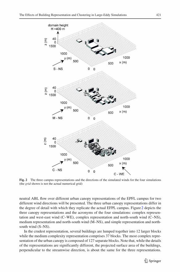
Fig. 2 The three campus representations and the directions of the simulated winds for the four simulations(the grid shown is not the actual numerical grid)

neutral ABL flow over different urban canopy representations of the EPFL campus for twodifferent wind directions will be presented. The three urban canopy representations differ inthe degree of detail with which they replicate the actual EFPL campus. Figure 2 depicts thethree canopy representations and the acronyms of the four simulations: complex represen-tation and west-east wind (C–WE), complex representation and north-south wind (C–NS),medium representation and north-south wind (M–NS), and simple representation and north-south wind (S–NS).

In the crudest representation, several buildings are lumped together into 12 larger blockswhile the medium complexity representation comprises 37 blocks. The most complex repre-sentation of the urban canopy is composed of 127 separate blocks. Note that, while the detailsof the representations are significantly different, the projected surface area of the buildings,perpendicular to the streamwise direction, is about the same for the three representations.

123


This detail will be important later in the analysis. The surfaces in the domain that are notcovered with buildings (green surface, roads, parking lots, etc.) are simply simulated as flatsurfaces with a prescribed roughness height (z0 = 0.1 m), as detailed in the wall model sectionabove. The dimensions of the domain are 1,500×1,500×400 m3, and the numerical grid forall simulations comprises 100×100×80 nodes. The grid spacing is hence 15 m in the twohorizontal directions and 5 m in the vertical direction (starting at 2.5 m due to the staggeredgrid). We simulated north-south winds for all building representation levels, and west-eastwinds only with the complex representation. Most of the campus buildings are oriented alongthe north-south direction and different flow patterns are hence expected with different winddirections.

If a typical value of 0.5 m s−1 is used for u∗, the timestep is 0.8 s (recalling that the codesolves normalised equations where u∗ does not need to be specified as input). All simulationsare integrated for 50,000 timesteps (excluding spin-up or warm-up time) representing around11.1 h of physical time to ensure robust statistical convergence, given that turbulent depar-tures are computed with respect to a time average, and higher order statistics are requiredfor the analysis. The campus roughly covers an area of 500×1,000 m, with most buildingheights between 15 and 20 m.

The focus of our analysis is mainly on qualitative comparisons between the different cam-pus representations. More accurate quantitative comparisons (which are not of great relevancesince they are very specific to the canopy being simulated), especially for the complex campusrepresentation, would require a higher grid resolution (see, for example, the discussion in Xieand Castro 2006). Nevertheless, domain size requirements for this study and computationalfeasibility prevent an increase in the numerical resolution at present. These simulations areusing 800,000 grid nodes in each simulation and hence the grid size is comparable to the sizeused in many recent LES studies. Since a doubling of the spatial resolution (which occurswith a halving of the timestep) requires eight times more floating point operations than thecurrent simulations (16 times if the total physical simulation time is to be preserved), it wouldnot be possible to increase the resolution significantly. One can attempt to increase the res-olution without increasing the number of grid points by reducing the domain size; however,when this was tested in the current study, it was detrimental to the quality of the results. Whena 200-m high domain was simulated (resulting in a doubling of the vertical resolution), weobserved that the flow was spuriously accelerated above the campus due to a severe restrictionof the flow cross-section (the top is a zero flow boundary). The blockage effect of the campuson the flow cross-section should be minimized, hence we had to maintain a domain heightof 400 m. On the other hand, the horizontal domain (Lx ) also cannot be reduced since it isrelated to the vertical domain size (Lz). One needs to maintain a horizontal domain size atleast four times greater than the vertical size (which will be the size of the largest eddies) ina periodic large-eddy simulation of the ABL to allow the eddies to evolve before exiting thedomain (see, for example, Moeng et al. 2007). In our simulations, we went just below thelimit of this ratio with an Lx/Lz = 3.75. In addition, a main objective is to look at the effectof aggregation of the buildings into clusters surrounded by smoother terrain. Hence we needto have an unbuilt area at least equal to that of the campus; this again prevents a reduction inthe horizontal size of the domain.

With these limitations on the attainable grid resolution, an assessment of the accuracy ofthe simulation results is needed to ensure that only the conclusions that can be reliably drawnfrom this study are addressed. As pointed out earlier, Tseng et al. (2006) showed that a gridresolution of about 63 nodes per cube was sufficient for a good match with experimentaldata using this code. Results with a lower resolution (43 nodes) did not match as well withexperimental results, but still captured the essential features of the flow. In our study, these

123


grid resolution requirements are critical for the complex representation of the campus. Whilemost buildings in the complex representation are captured with such a resolution of 43 nodesor better, the buildings have very complex shapes and aspect ratios and some details of thebuildings are not sufficiently resolved. However, the differences between the three campusrepresentations are extensive and most of these differences span more than 63 grid nodes.The differences between the representations are therefore well resolved. As such, despitethe relatively low resolution of each building detail, the qualitative comparative analysis isexpected to be reliable. Specifically, the results will indicate if the flow simulations are sen-sitive to the campus representation and will yield an estimate of this sensitivity, despite thefact that this estimate may not be highly accurate. The quantitative details anyway pertainonly to this specific urban canopy and are of little general interest. Similarly, later results (seebelow) reveal the general dynamics of the flow as it moves from the low-roughness terrainto the urban canopy and vice versa.

4 Roughness Length and Drag Coefficient of the Campus

The LES provides normalised velocity profiles (u/u∗) as a function of height; this infor-mation can be used to compute the displacement height d and the roughness length of thecampus z0 appearing as parameters in the law-of-the-wall velocity function, which appliesunder neutral conditions:

u

u∗= 1

κln

(z − d

z0

), (5)

where κ is the von Karman constant, u is the average velocity at height z, u∗ is the fric-tion velocity at the surface, and d is the displacement height. The velocity profiles used todetermine d and z0 were obtained by averaging the streamwise velocity data from the roofof the highest building on the campus (30 m) up to a height of 50 m. This height range wasselected to ensure that the internal boundary layer of the urban canopy is captured. The inflowadjustment zone (see code details above) was omitted from the averaging. Nevertheless, thearea around the campus was included since we want to determine the effective z0 and d forthe whole domain, and not just for the built-up areas. The z0 and d determined from theseaverage profiles will obviously depend on the size of the domain; this is an intentional out-come since the aim is to determine the effective aerodynamic parameters (see Bou-Zeid et al.2004, 2007) that would be used in a mesoscale model where the whole domain, including thespace around the campus, covers one grid cell. The simulated campus is a particular example,and we only analyze its results to answer the questions relating to the campus representationrequirements and the effect of wind direction.

In other applications, the aerodynamic properties of the built-up area alone (without sur-rounding flat surfaces) are of interest. Tests were performed for this study and confirmed thatthe resulting values of z0 and d indeed change with the averaging range. However, these testsalso indicated that the effects of building representation, which are the focus of this work, onthese aerodynamic properties are very similar regardless of the horizontal extent of profileaveraging.

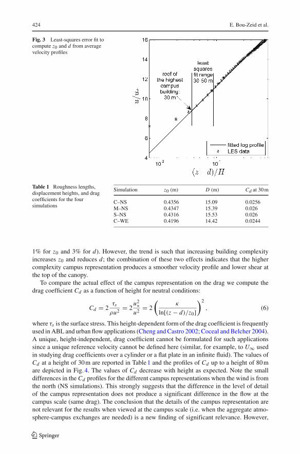
An example of the fit for the C–NW simulation is depicted in Fig. 3. A linear trend can bedetected in the lower 10% of the ABL (where the law-of-the-wall is expected to hold) downto the level of the highest campus roofs (≈30 m). The values of d and z0 obtained by thelinear fitting for all simulations are listed in Table 1. It is clear from the results that the effectof the campus representation details on the values of z0 and d is not very significant (about

123


Fig. 3 Least-squares error fit tocompute z0 and d from averagevelocity profiles

Table 1 Roughness lengths,displacement heights, and dragcoefficients for the foursimulations

Simulation z0 (m) D (m) Cd at 30 m

C–NS 0.4356 15.09 0.0256M–NS 0.4347 15.39 0.026S–NS 0.4316 15.53 0.026C–WE 0.4196 14.42 0.0244

1% for z0 and 3% for d). However, the trend is such that increasing building complexityincreases z0 and reduces d; the combination of these two effects indicates that the highercomplexity campus representation produces a smoother velocity profile and lower shear atthe top of the canopy.

To compare the actual effect of the campus representation on the drag we compute thedrag coefficient Cd as a function of height for neutral conditions:

Cd = 2τs

ρu2 = 2u2∗u2 = 2

(κ

ln[(z − d)/z0])2

, (6)

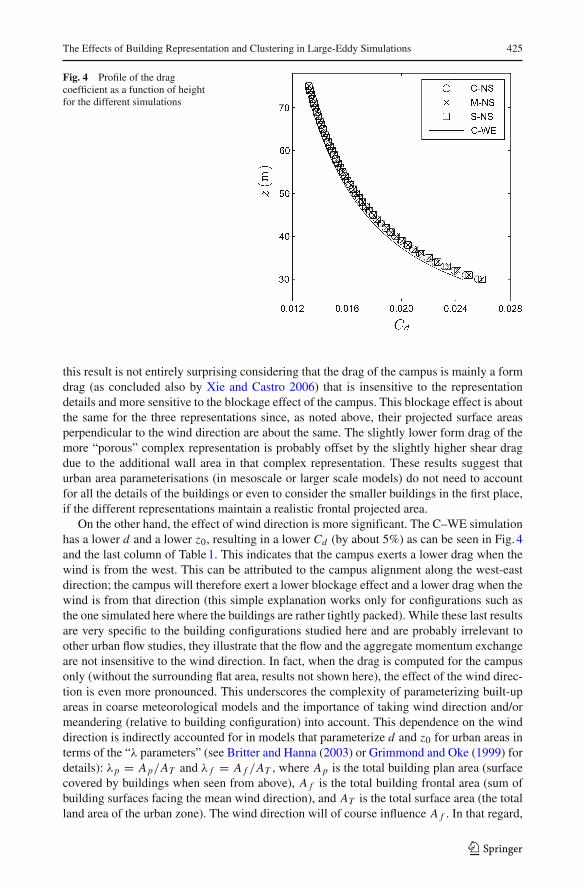
where τs is the surface stress. This height-dependent form of the drag coefficient is frequentlyused in ABL and urban flow applications (Cheng and Castro 2002; Coceal and Belcher 2004).A unique, height-independent, drag coefficient cannot be formulated for such applicationssince a unique reference velocity cannot be defined here (similar, for example, to U∞ usedin studying drag coefficients over a cylinder or a flat plate in an infinite fluid). The values ofCd at a height of 30 m are reported in Table 1 and the profiles of Cd up to a height of 80 mare depicted in Fig. 4. The values of Cd decrease with height as expected. Note the smalldifferences in the Cd profiles for the different campus representations when the wind is fromthe north (NS simulations). This strongly suggests that the difference in the level of detailof the campus representation does not produce a significant difference in the flow at thecampus scale (same drag). The conclusion that the details of the campus representation arenot relevant for the results when viewed at the campus scale (i.e. when the aggregate atmo-sphere-campus exchanges are needed) is a new finding of significant relevance. However,

123


Fig. 4 Profile of the dragcoefficient as a function of heightfor the different simulations

this result is not entirely surprising considering that the drag of the campus is mainly a formdrag (as concluded also by Xie and Castro 2006) that is insensitive to the representationdetails and more sensitive to the blockage effect of the campus. This blockage effect is aboutthe same for the three representations since, as noted above, their projected surface areasperpendicular to the wind direction are about the same. The slightly lower form drag of themore “porous” complex representation is probably offset by the slightly higher shear dragdue to the additional wall area in that complex representation. These results suggest thaturban area parameterisations (in mesoscale or larger scale models) do not need to accountfor all the details of the buildings or even to consider the smaller buildings in the first place,if the different representations maintain a realistic frontal projected area.

On the other hand, the effect of wind direction is more significant. The C–WE simulationhas a lower d and a lower z0, resulting in a lower Cd (by about 5%) as can be seen in Fig. 4and the last column of Table 1. This indicates that the campus exerts a lower drag when thewind is from the west. This can be attributed to the campus alignment along the west-eastdirection; the campus will therefore exert a lower blockage effect and a lower drag when thewind is from that direction (this simple explanation works only for configurations such asthe one simulated here where the buildings are rather tightly packed). While these last resultsare very specific to the building configurations studied here and are probably irrelevant toother urban flow studies, they illustrate that the flow and the aggregate momentum exchangeare not insensitive to the wind direction. In fact, when the drag is computed for the campusonly (without the surrounding flat area, results not shown here), the effect of the wind direc-tion is even more pronounced. This underscores the complexity of parameterizing built-upareas in coarse meteorological models and the importance of taking wind direction and/ormeandering (relative to building configuration) into account. This dependence on the winddirection is indirectly accounted for in models that parameterize d and z0 for urban areas interms of the “λ parameters” (see Britter and Hanna (2003) or Grimmond and Oke (1999) fordetails): λp = Ap/AT and λ f = A f /AT , where Ap is the total building plan area (surfacecovered by buildings when seen from above), A f is the total building frontal area (sum ofbuilding surfaces facing the mean wind direction), and AT is the total surface area (the totalland area of the urban zone). The wind direction will of course influence A f . In that regard,

123


a thorough testing of the “λ parameters” models for random building configurations and forwind directions that are not perpendicular to the faces of the buildings is needed and can beperformed using LES simulations as a benchmark.

5 Flow Adjustments Upstream, Over, and Downstream of the Campus

5.1 Mean Velocity Profiles

As air flows over the campus, both the mean flow and the turbulence are distorted by theinteraction with the buildings. In this section, we study this interaction for the north-southflow simulations since it is the only direction that allows us to clearly divide the domaininto upwind, over-the-campus, and downwind regions. We also omit the results from themedium complexity campus representation for clarity of presentation, but we verified thatthey invariably lie between the results of the simplest and most complex representations thatare presented here.

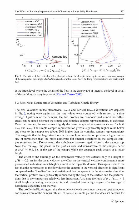
We start by analyzing the profiles of streamwise and vertical mean velocities upstream,over, and downstream of the campus; the averages are taken over fluid grid cells only, i.e. thezero fluid velocities in the buildings are not considered. In addition, we subtract the meanvertical profile of the velocities averaged over the whole domain to remove the strong meanvertical trends and emphasize the effect of the campus. These deviations from the mean pro-files are depicted in Fig. 5. The streamwise velocity over the campus is reduced significantlybelow the top of the buildings (z/H < 0.1) (Fig. 5a), it increases behind the campus, and at aheight of about twice the building heights (z/H = 0.2), it almost recovers its upstream pro-file. Note also the higher velocity at elevations of z/H > 0.1 over the campus. This speed-upabove the buildings is of course expected and compensates for the reduced velocity inside thecanopy as the atmospheric flow is diverted over the campus. The effect of this flow diversionover the campus is very clearly illustrated in the vertical velocity profiles of Fig. 5b. Upstreamfrom, and over, the campus, the flow is diverted upwards producing positive vertical velocityprofiles. A subsidence (negative vertical velocity) region is found behind the campus wherethe streamwise flow near the surface accelerates again, drawing air from above. It is inter-esting to note that in the upstream region, the flow is diverted downwards below the campustop and upwards above the campus top.

For the streamwise velocity profiles in Fig. 5a, the effect of the campus representationdetails is minimal. On the other hand, the variations due to campus representation aremore pronounced in the vertical velocities of Fig. 5b. This can be explained by the factthat the streamwise velocity profiles are strongly affected by the campus drag, which pro-duces significant departures from the domain mean (maximum difference of 1.3 m s−1)and the discrepancies due to the campus representation (root-mean-square (rms) difference≈0.048 m s−1) are small in comparison. On the other hand, for vertical velocities, the campusproduces maximum departures from the domain mean of about 0.12 m s−1 and the discrep-ancies due to the campus representation (rms difference ≈0.0073 m s−1) are relatively moresignificant.

The simple campus representation produces the largest upward flow deviation upstreamof the campus; while with the complex representation, (more porous canopy and more dis-tributed buildings) upwards flow deviation is more evenly divided between the upstream andover-the-campus zones. These results suggest that the effect of the campus representationcomplexity on the local simulated velocity profiles, while still small, is more important thanits effect on the profiles averaged over the whole domain (previous section). Obviously,

123


Fig. 5 Deviation of the vertical profiles of u and w from the domain mean upstream, over, and downstreamof the campus for the simple (dashed lines) and complex (solid lines) building representations and north-southflow

at the street level where the details of the flow in the canopy are of interest, the level of detailof the buildings is very important (Xie and Castro 2006).

5.2 Root-Mean Square (rms) Velocities and Turbulent Kinetic Energy

The rms velocities in the streamwise (urms) and vertical (wrms) directions are depictedin Fig. 6, noting once again that the rms values were computed with respect to a timeaverage. Upstream of the campus, the two profiles are “smooth” and almost no differ-ences can be noted between the simple and complex campus representations, as expected.Over the campus, the rms values slightly decrease compared to upstream values for bothurms and wrms. The simple campus representation gives a significantly higher value belowand close to the campus top (about 20% higher than the complex campus representation).This suggests that the large structures in the simple representation produce a higher inten-sity of turbulence than the more numerous but smaller structures in the complex cam-pus representation. Downstream, the turbulence increases again close to the canopy top.Note that for urms, the peaks in the profiles over and downstream of the campus occurat z/H ≈ 0.1, i.e. at the top of the canopy while the upstream peak occurs at a lowerheight.

The effect of the buildings on the streamwise velocity rms extends only to a height ofz/H ≈ 0.3. As for the mean velocity, the effect on the vertical velocity component is morepronounced and extends much higher, almost to the top of the domain. This again is due to thefact that the perturbation to the flow due to the campus in the vertical direction is significantcompared to the “baseline” vertical variation of that component. In the streamwise direction,the vertical profiles are significantly influenced by the drag at the surface and the perturba-tions due to the campus are relatively less important. Also note the ratio of urms/wrms > 1at all heights indicating, as expected in wall bounded flow, a high degree of anisotropy ofturbulence especially near the wall.

The profiles in Fig. 6 suggest that the turbulence levels are almost the same upstream, overand downstream of the campus. This is, of course, a simple picture that does not account for

123


Fig. 6 Normalised u and w rms velocities upstream, over, and downstream of the campus for the simple(dashed lines) and complex (solid lines) building representations with north-south winds

Fig. 7 x–z slice with TKE/u2∗ levels for simulation C–NS, averaged in time (over 11.1 h) and in the cross-stream direction; black rectangle delineates the extent of the campus

the rapid variation of the turbulent kinetic energy (TKE) over the campus. Figure 7 showsan x–z slice with the TKE values averaged in time and in the cross-stream (y) directionover and around the campus (which extends from 475 to 1,050 m in the x direction and upto 30 m in the z direction; the edges of the campus are delineated by the black rectanglein the figure). The contours are patchy due to cross-stream averaging over the non-uniformbuilding distributions. Note the very high TKE at the upstream edge of the campus (500 to650 m) and the significant reduction in the TKE as the flow velocity is reduced, and as thecampus drag and TKE cascade to the subgrid scales increase further downstream. Behindthe campus (x > 1,000 m), a smooth zone of high TKE is observed in the shear layer at theheight corresponding to building tops; the high TKE here is due to strong shear productionas will be illustrated later.

6 Stresses

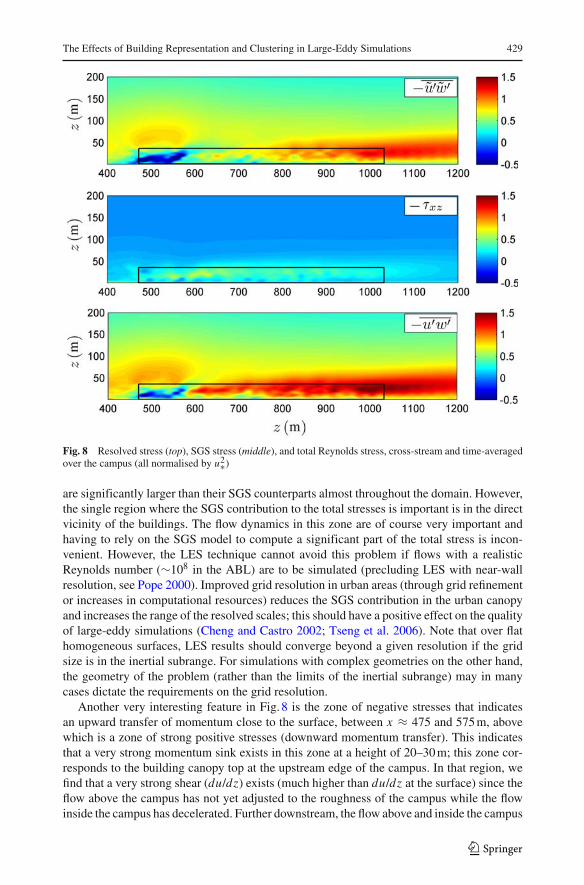
Figure 8 depicts the resolved, SGS, and total Reynolds stresses (sum of resolved and SGS) forthe complex representation (the other representations, as expected, gave similar trends sub-ject to the quantitative differences discussed in the previous sections). The resolved stresses

123


Fig. 8 Resolved stress (top), SGS stress (middle), and total Reynolds stress, cross-stream and time-averagedover the campus (all normalised by u2∗)

are significantly larger than their SGS counterparts almost throughout the domain. However,the single region where the SGS contribution to the total stresses is important is in the directvicinity of the buildings. The flow dynamics in this zone are of course very important andhaving to rely on the SGS model to compute a significant part of the total stress is incon-venient. However, the LES technique cannot avoid this problem if flows with a realisticReynolds number (∼108 in the ABL) are to be simulated (precluding LES with near-wallresolution, see Pope 2000). Improved grid resolution in urban areas (through grid refinementor increases in computational resources) reduces the SGS contribution in the urban canopyand increases the range of the resolved scales; this should have a positive effect on the qualityof large-eddy simulations (Cheng and Castro 2002; Tseng et al. 2006). Note that over flathomogeneous surfaces, LES results should converge beyond a given resolution if the gridsize is in the inertial subrange. For simulations with complex geometries on the other hand,the geometry of the problem (rather than the limits of the inertial subrange) may in manycases dictate the requirements on the grid resolution.

Another very interesting feature in Fig. 8 is the zone of negative stresses that indicatesan upward transfer of momentum close to the surface, between x ≈ 475 and 575 m, abovewhich is a zone of strong positive stresses (downward momentum transfer). This indicatesthat a very strong momentum sink exists in this zone at a height of 20–30 m; this zone cor-responds to the building canopy top at the upstream edge of the campus. In that region, wefind that a very strong shear (du/dz) exists (much higher than du/dz at the surface) since theflow above the campus has not yet adjusted to the roughness of the campus while the flowinside the campus has decelerated. Further downstream, the flow above and inside the campus

123


adjusts to the new surface, the shear is reduced, and the downwards momentum transfer ismore evenly distributed across the depth of the canopy. Towards the downstream edge of thecampus (after 800 m), the building density is reduced (see Fig. 2) and the flow acceleratesagain; strong downward momentum transfer is again observed as the ground becomes themain momentum sink.

The causes of this upward transfer of momentum at the leading edge are not the same asfor the upward transfer observed in forests (Lee and Black 1993), where the flow near thesurface (through the tree stems) has a higher velocity than the flow above (through the treecrowns) (Shaw 1977). In that case, the crowns act as a momentum sink and momentum istransferred from the stem zone to the crown zone possibly throughout the canopy. In ourstudy, the upward transfer is limited to the upstream edge of the campus. This local upwardmomentum transfer in building canopies is observed if the buildings are clustered into small“neighbourhoods” with low roughness areas in between. The effect of this horizontal vari-ability (acceleration and deceleration of the flow) on the dynamics of the atmospheric flowand on land-atmosphere exchanges in built-up areas has not been adequately studied to date.

7 TKE Budget over the Campus

The mean (overbar) resolved (tilde) turbulent kinetic energy (e) equation can be written as:

∂ e

∂t+ u j

∂ e

∂x j= −u′

i u′j∂ ui

∂x j− ∂ u′

j e

∂x j− 1

ρ

∂ u′j p′

∂x j− ∂ u′

iτ′i j

∂x j+ τ ′

i j S′i j + f ′

i u′i, (7)

where the overbar denotes Reynolds averaging, and was taken as the temporal mean over thewhole simulation in our analysis since spatial means are not well defined in complex domains(no spatial direction with homogeneous turbulence statistics). The prime denotes the turbu-lent component of the variable, and all other variables are as defined previously. The equationomits the buoyancy production or destruction term, which is not relevant for neutral flows,as well as the viscous dissipation, which is not significant at the scales resolved in LES withwall modelling. In our simulations, the unsteady term (∂/∂t) can be neglected since steadystate conditions are established. The two terms on the left represent the material derivativeof e. The first term on the right is the shear production or destruction, the second term is theturbulent transport, the third is the pressure transport, the fourth is the SGS transport, and thefifth is the “SGS dissipation”, i.e. the flux of TKE from the resolved to the subgrid scales.The last term is a sink of resolved TKE due to the force exerted by the buildings on the flow, fi .

We focus our attention on the shear production and SGS dissipation of TKE. Figure 9shows the time-averaged and cross-stream-averaged SGS dissipation, and as expected, SGS

Fig. 9 SGS dissipation (normalised), cross-stream and time-averaged, over the campus

123


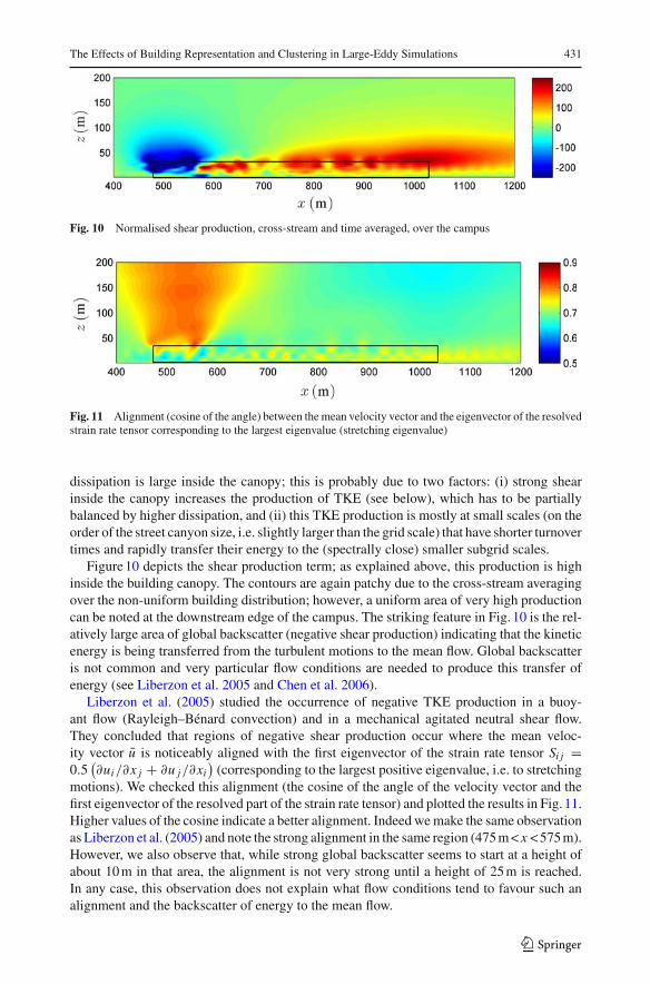
Fig. 10 Normalised shear production, cross-stream and time averaged, over the campus

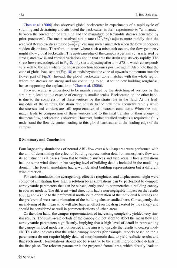
Fig. 11 Alignment (cosine of the angle) between the mean velocity vector and the eigenvector of the resolvedstrain rate tensor corresponding to the largest eigenvalue (stretching eigenvalue)

dissipation is large inside the canopy; this is probably due to two factors: (i) strong shearinside the canopy increases the production of TKE (see below), which has to be partiallybalanced by higher dissipation, and (ii) this TKE production is mostly at small scales (on theorder of the street canyon size, i.e. slightly larger than the grid scale) that have shorter turnovertimes and rapidly transfer their energy to the (spectrally close) smaller subgrid scales.

Figure 10 depicts the shear production term; as explained above, this production is highinside the building canopy. The contours are again patchy due to the cross-stream averagingover the non-uniform building distribution; however, a uniform area of very high productioncan be noted at the downstream edge of the campus. The striking feature in Fig. 10 is the rel-atively large area of global backscatter (negative shear production) indicating that the kineticenergy is being transferred from the turbulent motions to the mean flow. Global backscatteris not common and very particular flow conditions are needed to produce this transfer ofenergy (see Liberzon et al. 2005 and Chen et al. 2006).

Liberzon et al. (2005) studied the occurrence of negative TKE production in a buoy-ant flow (Rayleigh–Bénard convection) and in a mechanical agitated neutral shear flow.They concluded that regions of negative shear production occur where the mean veloc-ity vector u is noticeably aligned with the first eigenvector of the strain rate tensor Si j =0.5

(∂ui/∂x j + ∂u j/∂xi

)(corresponding to the largest positive eigenvalue, i.e. to stretching

motions). We checked this alignment (the cosine of the angle of the velocity vector and thefirst eigenvector of the resolved part of the strain rate tensor) and plotted the results in Fig. 11.Higher values of the cosine indicate a better alignment. Indeed we make the same observationas Liberzon et al. (2005) and note the strong alignment in the same region (475 m < x < 575 m).However, we also observe that, while strong global backscatter seems to start at a height ofabout 10 m in that area, the alignment is not very strong until a height of 25 m is reached.In any case, this observation does not explain what flow conditions tend to favour such analignment and the backscatter of energy to the mean flow.

123


Chen et al. (2006) also observed global backscatter in experiments of a rapid cycle ofstraining and destraining and attributed the backscatter in their experiments to “a mismatchbetween the orientation of straining and the magnitude of Reynolds stresses generated byprior processes”. The mean resolved strain rate (∂ ui/∂x j ) adjusts more rapidly than the

resolved Reynolds-stress tensor (−u′i u

′j ), causing such a mismatch when the flow undergoes

sudden distortions. Therefore, in zones where such a mismatch occurs, the flow geometrymight allow global backscatter. The upstream edge of the campus is certainly characterised bystrong streamwise and vertical variations and in that area the strain adjusts very rapidly. Thestress however, as depicted in Fig. 8, only starts adjusting after x ≈ 575 m, which correspondsvery well to the area where the shear production becomes positive again. Also note that thezone of global backscatter (Fig. 10) extends beyond the zone of upwards momentum transfer(lower part of Fig. 8). Instead, the global backscatter zone matches with the whole regionwhere the stresses are strong and are continuing to adjust to the new building roughness,hence supporting the explanation of Chen et al. (2006).

Forward scatter is understood to be mainly caused by the stretching of vortices by thestrain rate, leading to a cascade of energy to smaller scales. Backscatter, on the other hand,is due to the compression of these vortices by the strain rate in the fluid. At the lead-ing edge of the campus, the strain rate adjusts to the new flow geometry rapidly whilethe stresses and vortices are still representative of upstream conditions. When the mis-match leads to compression of these vortices and to the final transfer of their energy tothe mean flow, backscatter is observed. However, further detailed analysis is required to fullyunderstand the flow dynamics leading to this global backscatter at the leading edge of thecampus.

8 Summary and Conclusion

Four large-eddy simulations of neutral ABL flow over a built-up area were performed withthe aim of determining the effect of building representation detail on atmospheric flow andits adjustment as it passes from flat to built-up surfaces and vice versa. Three simulationshad the same wind direction but varying level of building details included in the modellingdomain. The fourth simulation had a well-detailed building representation but a differentwind direction.

For each simulation, the average drag, effective roughness, and displacement height werecomputed illustrating how high resolution local simulations can be performed to computeaerodynamic parameters that can be subsequently used to parameterize a building canopyin coarser models. The different wind directions had a non-negligible impact on the results(Cd , zo and d) due to the preferential north-south orientation of the individual buildings andthe preferential west-east orientation of the building cluster studied here. Consequently, themeandering of the mean wind will also have an effect on the drag exerted by the canopy andshould be considered as well in parameterisations of urban areas.

On the other hand, the campus representations of increasing complexity yielded very sim-ilar results. The small-scale details of the canopy did not seem to affect the mean flow andaerodynamic parameters significantly, implying that a high level of detail in representingthe canopy in local models is not needed if the aim is to upscale the results to coarser mod-els. This also indicates that the urban canopy models (for example, models based on the λ

parameters) do not require highly detailed morphometric data to yield realistic results andthat such model formulations should not be sensitive to the small morphometric details inthe first place. The relevant parameter is the projected frontal area, which directly leads to

123


flow blockage and form drag. Our different models of the urban canopy were constructed tohave very similar projected frontal areas, and our conclusions are therefore only confirmedunder such conditions.

The mean velocity profiles upstream, over, and downstream of the building cluster forthe different simulations were also analyzed and indicated moderate differences betweenthe simulations with different campus representations. For the turbulent components, how-ever, the effect of the different campus representations was more important, with differencesbetween the campus models reaching up to 20 percent. The vertical components of both themean and turbulent velocities were found to be more sensitive to the campus representationthan the streamwise components. Analysis of the stresses indicates that the subgrid-scale partis important in and close to the campus.

This suggests that inclusion of a high level of detail in a building representation remainsimportant in local models if the aim is to simulate the flow and the transport of pollutants atthe street or canopy scale. For such simulations, the highest attainable grid resolution shouldbe used all through the urban canopy (not just over the buildings). This will have a positiveeffect on the grid resolution of the buildings and at the same time will reduce the modelledSGS fraction of the turbulent stresses, allowing more turbulent scales to be directly resolved.However, morphometric data might often be available at a resolution that cannot be capturedin the local simulation due to grid resolution restrictions. In such instances, regardless ofthe aim of the simulation (upscaling or local flow dynamics), we recommend constructingthe simplified version of the canopy so as to have the same λ parameters as the high-detailmorphometric data.

This study also investigated the flow adjustment from a flat/vegetated to a built-up areaand back to a flat/vegetated area. The TKE was shown to be very high at the upstream edgeof the campus and to decrease very rapidly as the air flows through the building canopy,only to increase again downstream from the campus. The shear production and dissipationof the TKE were also analyzed and a region with strong “global backscatter” was observedat the upstream edge of the campus, indicating a transfer of energy from the turbulence tothe mean flow. The global backscatter can be attributed to a mismatch (imbalance) of thestrain and the stress in the flow that occurs when sudden perturbations are imposed. This,along with the strong variations in the velocities, stresses, and TKE as the air flows over thebuilding cluster, underlines the importance of including surface variability in urban canopymodels.

At present, most urban canopy models are based exclusively on the properties of thecanopy and exclude the effect of the surroundings; therefore, the effects of these strongstreamwise flow variations are not included in these models. These variations, and hencethe horizontal spatial scale of the urban canopy, will have an important effect on the can-opy-atmosphere exchange rates, just as with variable natural terrain (Bou-Zeid et al. 2007).Therefore, a heterogeneous suburban canopy cannot be adequately parameterised withoutconsideration of its subgrid spatial variability, relative to the grids of regional or globalatmospheric models.

Acknowledgements The authors would like the thank the Swiss National Science Foundation for its sup-ports for this work through grant number 200021-107910 and through the National Competence Centre inResearch on Mobile Information and Communication Systems (NCCR-MICS) under grant number 5005-67322. Professor Bou-Zeid was also supported by the High Meadows Sustainability Fund through the “SensorNetwork over Princeton” project. The authors are also grateful to the Swiss National Supercomputing Cen-tre for its support and allocation of ample computing resources for the simulations of this paper. ProfessorCharles Meneveau’s and Professor Yu-Heng Tseng’s contributions to the development of the code and to theimplementation of the immersed boundary method are also greatly appreciated.

123


References

Albertson JD, Parlange MB (1999a) Natural integration of scalar fluxes from complex terrain. Adv WaterResour 23(3):239–252

Albertson JD, Parlange MB (1999b) Surface length scales and shear stress: implications for land–atmosphereinteraction over complex terrain. Water Resour Res 35(7):2121–2132

Albertson JD, Kustas WP, Scanlon TM (2001) Large-eddy simulation over heterogeneous terrain withremotely sensed land surface conditions. Water Resour Res 37(7):1939–1953

Avissar R (1995) Recent advances in the representation of land–atmosphere interactions in general-circulationmodels. Rev Geophys 33:1005–1010

Belcher SE, Jerram N, Hunt JCR (2003) Adjustment of a turbulent boundary layer to a canopy of roughnesselements. J Fluid Mech 488:369–398

Bou-Zeid E, Meneveau C, Parlange MB (2004) Large-eddy simulation of neutral atmospheric boundary layerflow over heterogeneous surfaces: blending height and effective surface roughness. Water Resour Res40(2):W02505. doi:10.1029/2003WR002475

Bou-Zeid E, Meneveau C, Parlange MB (2005) A scale-dependent Lagrangian dynamic model for large eddysimulation of complex turbulent flows. Phys Fluids 17(2):025105. doi:10.1063/1.1839152

Bou-Zeid E, Parlange MB, Meneveau C (2007) On the parameterization of surface roughness at regionalscales. J Atmos Sci 64(1):216–227. doi:10.1175/JAS3826.1

Bou-Zeid E, Vercauteren N, Parlange MB, Meneveau C (2008) Scale dependence of subgrid-scale modelcoefficients: an a priori study. Phys Fluids 20(11):115106

Bradbrook KF, Lane SN, Richards KS, Biron PM, Roy AG (2000) Large eddy simulation of periodic flowcharacteristics at river channel confluences. J Hydraul Res 38(3):207–215

Britter RE, Hanna SR (2003) Flow and dispersion in urban areas. Annu Rev Fluid Mech 35:469–496Brutsaert W (1998) Land-surface water vapor and sensible heat flux: spatial variability, homogeneity, and

measurement scales. Water Resour Res 34(10):2433–2442. doi:10.1029/98WR01340Cai XM (1999) Large-eddy simulation of the convective boundary layer over an idealized patchy urban sur-

face. Q J Roy Meteorol Soc 125(556):1427–1444Calhoun R, Gouveia F, Shinn J, Chan S, Stevens D, Lee R, Leone J (2005) Flow around a complex building:

experimental and large-eddy simulation comparisons. J Appl Meteorol 44(5):571–590Celani A (2007) The frontiers of computing in turbulence: challenges and perspectives. J Turbul 8(1):1–9Chen J, Meneveau C, Katz J (2006) Scale interactions of turbulence subjected to a straining–relaxation–

destraining cycle. J Fluid Mech 562:123–150Cheng H, Castro IP (2002) Near wall flow over urban-like roughness. Boundary-Layer Meteorol 104(2):

229–259Coceal O, Belcher SE (2004) A canopy model of mean winds through urban areas. Q J Roy Meteorol Soc

130(599):1349–1372Dupont S, Mestayer PG (2006) Parameterization of the urban energy budget with the submesoscale soil model.

J Appl Meteorol Clim 45(12):1744–1765Eliasson I, Offerle B, Grimmond CSB, Lindqvist S (2006) Wind fields and turbulence statistics in an urban

street canyon. Atmos Environ 40(1):1–16Emeis S (2004a) Parameterization of turbulent viscosity over orography. Meteorol Z 13(1):33–38Emeis S (2004b) Vertical wind profiles over an urban area. Meteorol Z 13(5):353–359Emeis S, Turk M (2004) Frequency distributions of the mixing height over an urban area from SODAR data.

Meteorol Z 13(5):361–367Germano M, Piomelli U, Moin P, Cabot WH (1991) A dynamic subgrid-scale eddy viscosity model. Phys

Fluids A 3(7):1760–1765Grimmond CSB, Oke TR (1999) Aerodynamic properties of urban areas derived, from analysis of surface

form. J Appl Meteorol 38(9):1262–1292Grimmond CSB, King TS, Roth M, Oke TR (1998) Aerodynamic roughness of urban areas derived from wind

observations. Boundary-Layer Meteorol 89(1):1–24Harman IN, Belcher SE (2006) The surface energy balance and boundary layer over urban street canyons.

Q J Roy Meteorol Soc 132(621):2749–2768Kanda M, Moriwaki R, Kasamatsu F (2004) Large-eddy simulation of turbulent organized structures within

and above explicitly resolved cube arrays. Boundary-Layer Meteorol 112(2):343–368Keylock CJ, Hardy RJ, Parsons DR, Ferguson RI, Lane SN, Richards KS (2005) The theoretical foundations

and potential for large-eddy simulation (LES) in fluvial geomorphic and sedimentological research. EarthSci Rev 71(3–4):271–304

123

http://dx.doi.org/10.1029/2003WR002475

http://dx.doi.org/10.1063/1.1839152

http://dx.doi.org/10.1175/JAS3826.1

http://dx.doi.org/10.1029/98WR01340


Kleissl J, Kumar V, Meneveau C, Parlange MB (2006) Numerical study of dynamic Smagorinsky models inlarge-eddy simulation of the atmospheric boundary layer: validation in stable and unstable conditions.Water Resour Res 42(6):W06D10. doi:10.1029/2005WR004685

Kumar V, Kleissl J, Meneveau C, Parlange MB (2006) Large-eddy simulation of a diurnal cycle of the atmo-spheric boundary layer: atmospheric stability and scaling issues. Water Resour Res 42(6):W06D09.doi:10.1029/2005WR004651

Lee XH, Black TA (1993) Atmospheric-turbulence within and above a Douglas–Fir stand. 1. Statistical prop-erties of the velocity-field. Boundary-Layer Meteorol 64(1-2):149–174

Liberzon A, Luthi B, Guala M, Kinzelbach W, Tsinober A (2005) Experimental study of the structure of flowregions with negative turbulent kinetic energy production in confined three-dimensional shear flows withand without buoyancy. Phys Fluids 17(9):095110

Lilly DK (1967) The representation of small scale turbulence in numerical simulation experiments. In: IBMscientific computing symposium on environmental sciences, White Plains, New York, pp 195–209

Lin CL, Glendening JW (2002) Large eddy simulation of an inhomogeneous atmospheric boundary layerunder neutral conditions. J Atmos Sci 59(16):2479–2497

Lyn DA, Rodi W (1994) The flapping shear-layer formed by flow separation from the forward corner of asquare cylinder. J Fluid Mech 267:353–376

Masson V (2000) A physically-based scheme for the urban energy budget in atmospheric models. Boundary-Layer Meteorol 94(3):357–397

Meinders ER, Hanjalic K (1999) Vortex structure and heat transfer in turbulent flow over a wall-mountedmatrix of cubes. Int J Heat Fluid Flow 20(3):255–267

Meinders ER, Hanjalic K (2002) Experimental study of the convective heat transfer from in-line and staggeredconfigurations of two wall-mounted cubes. Int J Heat Mass Transf 45(3):465–482

Meneveau C, Katz J (2000) Scale-invariance and turbulence models for large-eddy simulation. Annu RevFluid Mech 32:1–32

Meneveau C, Lund TS, Cabot WH (1996) A Lagrangian dynamic subgrid-scale model of turbulence. J FluidMech 319:353–385

Moeng CH, Dudhia J, Klemp J, Sullivan P (2007) Examining two-way grid nesting for large eddy simulationof the PBL using the WRF model. Mon Weather Rev 135(6):2295–2311

Molod A, Salmun H, Waugh DW (2003) A new look at modeling surface heterogeneity: extending its influencein the vertical. J Hydrometeorol 4(5):810–825

Monin AS, Obukhov AM (1954) Basic laws of turbulent mixing in the ground layer of the atmosphere (inRussian), vol 151. Trudy Geofizicheskogo Instituta, Akademiya Nauk SSSR, pp 163–187

Orszag SA, Pao YH (1974) Numerical computation of turbulent shear flows. Adv Geophys 18(A):224–236Parlange MB, Brutsaert W (1993) Regional shear-stress of broken forest from radiosonde wind profiles in the

unstable surface-layer. Boundary-Layer Meteorol 64(4):355–368Piomelli U (1999) Large-eddy simulation: achievements and challenges. Prog Aerosp Sci 35(4):335–362Pope SB (2000) Turbulent flows. Cambridge University Press, Cambridge, 771 ppPorte-Agel F, Meneveau C, Parlange MB (2000) A scale-dependent dynamic model for large-eddy simulation:

application to a neutral atmospheric boundary layer. J Fluid Mech 415:261–284Roberts SM, Oke TR, Grimmond CSB, Voogt JA (2006) Comparison of four methods to estimate urban heat

storage. J Appl Meteorol Clim 45(12):1766–1781Rotach MW, Fisher B, Piringer M (2002) COST 715 workshop on urban boundary layer parameterizations.

Bull Am Meteorol Soc 83(10):1501–1504Roth M (2000) Review of atmospheric turbulence over cities. Q J Roy Meteorol Soc 126(564):941–990Roth M, Salmond JA, Satyanarayana ANV (2006) Methodological considerations regarding the measurement

of turbulent fluxes in the urban roughness sublayer: the role of scintillometery. Boundary-Layer Meteorol121(2):351–375

Roulet YA, Martilli A, Rotach MW, Clappier A (2005) Validation of an urban surface exchange parameteri-zation for mesoscale models—1D case in a street canyon. J Appl Meteorol 44(9):1484–1498

Sagaut P (2003) Large eddy simulation for incompressible flows. Springer, Berlin, 426 ppShaw RH (1977) Secondary wind speed maxima inside plant canopies. J Appl Meteorol 16(5):514–521Shen L, Yue DKP (2001) Large-eddy simulation of free-surface turbulence. J Fluid Mech 440:75–116Smagorinsky J (1963) General circulation experiments with the primitive equations: I. the basic experiment.

Mon Weather Rev 91:99–164Stoll R, Porte-Agel F (2006) Dynamic subgrid-scale models for momentum and scalar fluxes in large-eddy

simulations of neutrally stratified atmospheric boundary layers over heterogeneous terrain. Water ResourRes 42(1):W01409

Tominaga Y, Mochida A, Murakami S, Sawaki S (2008) Comparison of various revised k-[epsilon] modelsand LES applied to flow around a high-rise building model with 1:1:2 shape placed within the surfaceboundary layer. J Wind Eng Ind Aerodyn 96(4):389–411

123

http://dx.doi.org/10.1029/2005WR004685

http://dx.doi.org/10.1029/2005WR004651


Tseng YH, Meneveau C, Parlange MB (2006) Modeling flow around bluff bodies and predicting urbandispersion using large eddy simulation. Environ Sci Technol 40(8):2653–2662

Wood N (2000) Wind flow over complex terrain: a historical perspective and the prospect for large-eddymodelling. Boundary-Layer Meteorol 96(1-2):11–32

Xie ZT, Castro IP (2006) LES and RANS for turbulent flow over arrays of wall-mounted obstacles. FlowTurbul Combust 76(3):291–312

Xie ZT, Li JC (2005) A numerical study for turbulent flow and thermal influence over inhomogenous canopyof roughness elements. Environ Fluid Mech 5(6):577–597

Yue WS, Meneveau C, Parlange MB, Zhu WH, van Hout R, Katz J (2007a) A comparative quadrant analysisof turbulence in a plant canopy. Water Resour Res 43(5):W05422. doi:10.1029/2006WR005583

Yue WS, Parlange MB, Meneveau C, Zhu WH, van Hout R, Katz J (2007b) Large-eddy simulation of plantcanopy flows using plant-scale representation. Boundary-Layer Meteorol 124(2):183–203

Zhang N, Jiang WM, Miao SG (2006) A large eddy simulation on the effect of buildings on urban flows. WindStruct 9(1):23–35

123

http://dx.doi.org/10.1029/2006WR005583

Documents

The Effects of Building Representation and Clustering in Large-Eddy Simulations of Flows in Urban Canopies