Latent Dirichlet Co-Clustering

M. Mahdi Shafiei and Evangelos E. MiliosFaculty of Computer Science, Dalhousie University

6050 University Ave., Halifax, Canadashafiei@cs.dal.ca , eem@cs.dal.ca

Abstract

We present a generative model for simultaneously clus-tering documents and terms. Our model is a four-levelhierarchical Bayesian model, in which each document ismodeled as a random mixture of document topics , whereeach topic is a distribution over some segments of the text.Each of these segments in the document can be modeledas a mixture of word topics where each topic is a distri-bution over words. We present efficient approximate in-ference techniques based on Markov Chain Monte Carlomethod and a Moment-Matching algorithm for empiricalBayes parameter estimation. We report results in docu-ment modeling, document and term clustering, comparingto other topic models, Clustering and Co-Clustering algo-rithms including Latent Dirichlet Allocation (LDA), Model-based Overlapping Clustering (MOC), Model-based Over-lapping Co-Clustering (MOCC) and Information-TheoreticCo-Clustering (ITCC).

1 Introduction

Finding the appropriate representation model for textdata has been one of the main issues for the data min-ing community since it started to look at the problem ofprocessing text automatically. The “bag-of-words” repre-sentation is the basic and most widely used representationmethod for textual data [19]. In this approach, the order ofwords at which they appear in documents are ignored andonly the word frequencies are taken into account. But thisapproach has been criticized for several reasons. Amongthose, it provides a relatively high dimensional represen-tation of data (equal to the dictionary size) which causescurse of dimensionality problem [19]. Furthermore, it doesnot consider synonymy and polysemy relations of words innatural language. It has been also criticized of losing infor-mation due to its ignorance of word order. Various prepro-cessing steps such as removing stop-words and stemminghave been used to reduce dimensionality, create and select

better features.

To overcome the high dimensionality issue of the bag-of-words representation, several dimension reduction methodshave been proposed. Feature selection methods select a sub-set of words to reduce the dimensionality. Feature transfor-mation methods try to tackle not only the high dimensional-ity problem of “bag-of-words” representation, but indirectlyconsider synonymy and polysemy as well. Latent SemanticIndexing (LSI) [6] is one of these approaches which usessingular value decomposition to identify a linear subspacein the original space of features. It is believed that the result-ing new features also capture the two mentioned propertiesof natural language - polysemy and synonymy.

But the problem with most cartesian space representationapproaches for text like LSI is their inability to provide in-terpretable components. Despite some work on interpretingthe dimensions generated by these methods [5], these ap-proaches are still far from providing a natural interpretationin the case of text. Topic models, on the other hand, are aclass of statistical models in which the semantic propertiesof words and documents are expressed in terms of proba-bilistic topics. Probabilistic topic modeling as a way of rep-resenting the content of words and documents has the dis-tinct advantage that each topic is individually interpretable,providing a probability distribution over words that picksout a coherent cluster of correlated terms. The major dif-ference between cartesian space methods like LSI and sta-tistical topic models is that LSI family methods claim thatwords and documents can be represented as points in theEuclidean space whereas for the topic models, this is notthe case.

One common assumption among most statistical modelsfor language is still the bag-of-words assumption. In thesemodels, no assumption is made about the order of words. Inother words, while this family of methods tries to deal withthe two first issues of bag-of-words representation, high di-mensionality and ignoring polysemy and synonymy prop-erties, it still keeps the “bag-of-words” assumption intact.Recently, there has been increased research interest in mod-els sensitive to this kind of information [11].

Proceedings of the Sixth International Conference on Data Mining (ICDM'06)0-7695-2701-9/06 $20.00 © 2006

The basic idea behind all proposed topic models [10, 3]is that a document is a mixture of several topics where eachtopic is some distribution over words. Each topic model is agenerative model which specifies a simple probabilistic pro-cess by which the words in a document are being generatedon the basis of a small number of latent variables.

Using standard statistical techniques, one can invert theprocess and infer the set of latent variables responsible forgenerating a given set of documents [21]. Assuming amodel for generating the data, the goal of fitting this gen-erative model is to find the best set of latent variables thatcan explain the observed data (i.e., observed words in doc-uments).

Probabilistic Latent Semantic Analysis (also known asthe aspect model) [12] was one of the first attempts towardusing probabilistic models for document and text modeling.In this model, each word is assumed to be a sample from amixture model. Mixture components are multinomial ran-dom variables that can be viewed as representations of “top-ics”. Each word is generated from a single topic and a doc-ument is a collection of words generated potentially fromdifferent topics.

Though a useful step after LSI, the PLSI model doesnot provide a generative model for a document, instead itis a model for word/document co-occurrences [13]. Thisassumption makes it difficult to assign probabilities to doc-uments outside of the learning corpus. Latent Dirichlet Al-location [3], on the contrary, is a true generative model fordocuments and therefore provides the means for generatingboth the observed and unseen documents. In LDA, the doc-uments are assumed to be sampled from a random mixtureover latent topics, where each topic is characterized by adistribution over words. Furthermore, the mixture coeffi-cients are also assumed to be random and by considering aprior probability on them, LDA provides a complete gener-ative model for the documents [10].

In Latent Dirichlet Allocation, a document is gener-ated by first picking a distribution over latent topics froma Dirichlet distribution, which determines the multinomialdistribution over topics for words in that document. Thewords in the document are then generated by picking a topicfor each word from this distribution and then picking a wordfrom that topic according to another multinomial distribu-tion. Fig. 1.b shows the graphical model corresponding tothe generative model of LDA.

The major and direct output of these models is a set ofoverlapping clusters of words. Clustering documents canbe viewed only as a byproduct and not as a direct output oftopic models. On the other hand, co-clustering [8, 20, 15]is a data mining technique with various applications suchas text clustering and microarray analysis. Co-clusteringalgorithms try to simultaneously cluster rows and columnsof a two-dimensional data matrix. One of the benefits of

co-clustering algorithms is taking advantage of the dual-ity between documents and words and in general the du-ality between the rows and columns of an adjacency ma-trix. Co-clustering algorithms, using the clustering resultson words as a low dimensional representation of documentscan achieve a more accurate clustering for documents [8].In this work, we try to combine these two ideas, proba-bilistic topic models and co-clustering, using topic mod-els to construct a low-dimensional representation of docu-ments. Therefore, we extend the original idea of topic mod-els to consider the resulting low-dimensional representationof documents in another nested topic model for clusteringdocuments.

The topics discovered by most probabilistic topic modelscapture the correlation between words, but the correlationsbetween topics are not modeled. Several models have beenrecently proposed to capture the correlation between topics,such as Hierarchical Dirichlet Processes Model (HDP) [22],Correlated Topic Models (CTM) [2] and Pachinko Alloca-tion Model (PAM) [14]. In natural text data, it is commonto have correlations among topics. As pointed out in [2],“a document about sports is more likely to also be abouthealth than international finance”. In the LDA model, thetopic proportions are derived from a Dirichlet distributionand hence are nearly independent. CTM tries to capturetopic correlations by introducing logistic normal distribu-tion instead of Dirichlet distribution for drawing topic mix-ture proportions. The logistic normal distribution is yetagain a distribution on the simplex where the correlationbetween pairs of components is described through a covari-ance matrix. In CTM, only the pairwise correlations aremodeled and the number of parameters grows quadraticallywith the number of topics [14]. In the PAM model, similarto our proposed model, the concept of topic is extended toinclude not only distributions over words, but also distribu-tion over topics. The model structure is an arbitrary DAGwhere each leaf is associated with a word and each non-leafnode is a distribution over its children. The direct parents ofthe leaf nodes are distributions over words and correspondto topics in LDA. All other interior nodes are distributionsover topics and called “super-topics”. Allowing an arbitraryDAG structure, the PAM model is able to capture arbitrarycorrelations between word topics.

In this paper, we propose a generative model for text doc-uments based on LDA model which is able to cluster bothwords and documents simultaneously. The model is alsomore sensitive to to the locations of words in documents byfocusing on meaningful segments of text. This enables themodel to detect multiple topics covered by a document.

The rest of this paper is organized as follows. In sec-tion 2, we present the Latent Dirichlet Co-Clustering Model(LDCC). We propose inference and parameter estimationalgorithms for LDCC in Section 3. Finally, we conclude the

Proceedings of the Sixth International Conference on Data Mining (ICDM'06)0-7695-2701-9/06 $20.00 © 2006

paper with a brief review of the paper and some discussionon future works in section 5.

2 Latent Dirichlet Co-Clustering Model

We use the same notation and definitions as in [3]. Wedefine the following terms:

• A word is the basic building block of our data and itis selected from a vocabulary indexed by {1, . . . , V }.We represent words using unit-basis vectors that havea single component equal to one and all other compo-nents equal to zero. Thus, the vth word in the vocab-ulary is represented by a V -vector w such that the vthcomponent is one and all other components are zero.

• A document is a sequence of words w =(w1, w2, . . . , wN ), where N is the number of wordsin the document.

• A corpus is a collection of M documents denoted byD = {w1, w2, . . . , wM}

The basic idea of the LDA model is to assume each doc-ument as a random mixture over latent topics, where eachtopic is specified by a distribution over words. We extendthis idea by assuming each document is a random mixtureof topics , where each topic is a distribution over some seg-ments of the document. Now, each of these segments in thedocument can be modeled by LDA.

The intuition behind this work is that documents arecomposed of meaningful single-topic segments put to-gether. Each of these segments is assumed to convey a sin-gle concept or topic. This topic is among a handful of top-ics which specifies the theme of the document. If one looksat each of these segments separately, the order of words inthe segment is assumed to have little impact on the conceptwhich the segment is trying to convey. Thus, the “bag-of-words” assumption for these segments is fairly realistic, un-like for the whole document. In this work, we assume seg-ments are paragraphs of the text. The proposed model triesto model each segment based on its word content similar tomost probabilistic topic models. Then these learned topicson the words are being used to represent document topics.In other words, each document topic is considered a mix-ture of word topics where the mixture coefficients uniquelyspecifies the document topic.

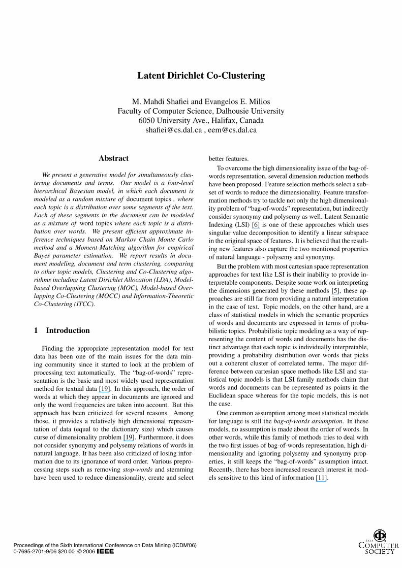
The generative probabilistic model we propose is shownas a graphical model in Fig. 1. Plate notation [4] is a stan-dard and convenient way of illustrating probabilistic gener-ative models with repeated sampling steps. In this graphicalnotation, shaded and unshaded variables indicate observedand latent (i.e., unobserved) variables respectively.

α

β

δ

φ

y

θ

z

w

N

S

M

η

L

(a) Co-Clustering Model

α

β

θ

z

w

N

M

η

L

(b) LDA Model

Figure 1. LDA Model and Co-ClusteringModel inspired by LDA

The LDCC model assumes the following generative pro-cess for each document d in a corpus D (intuitive explana-tions of model parameters are given in the text following theoverview of the generative process.):

1. Choose S ∼ Poisson(µ) : number of segments (para-graphs or sentences) in the document

2. Choose φ ∼ Dir(δ)

3. For each of the S segments s

(a) Choose a topic for the segment ys ∼Multinomial(φ)

(b) Choose Ns ∼ Poisson(ε) : number of words inthe segment

(c) Choose θs ∼ Dir(α, ys)

(d) For each of the Ns words wsn

i. Choose a topic zsn ∼ Multinomial(θs)ii. Choose a word wsn from P (wsn|zsn, β), a

multinomial probability conditioned on thetopic zsn

We have assumed that the number of word and documenttopics (and hence the dimensionality of topic variables zand y) are known and fixed. We also model the word proba-bilities conditioned on the topics by a L×V matrix β whereβij = p(wj = 1|zi = 1) which is assumed to be fixed andwill be estimated though the learning process. Finally, asin the LDA model, we can use any other document length

Proceedings of the Sixth International Conference on Data Mining (ICDM'06)0-7695-2701-9/06 $20.00 © 2006

distribution instead of the Poisson distribution as it is notimportant for the rest of the model. Furthermore, note thatthe Ns variables are independent of all the other data gen-erating variables (θ, z, φ and y) and we therefore ignore itsrandomness in the subsequent development.

Note that φ represents the mixing proportion ofdocument-topics in a document. It specifies the parametersof the K-dimensional multinomial distribution from whichthe model draws samples for document topics. θs is a sam-ple from the Dirichelt distribution and specifies the mixingproportion of word-topics in the text segment s. Note thatthis mixing proportion depends on the document-topic thatthe current text segment is generated from. The model as-sume that each document-topic is a mixture of several word-topics and this fact is modeled through the matrix of hyper-parameters α.

The Dirichlet distribution is a conjugate prior for themultinomial distribution. Choosing a conjugate prior makesthe problem of statistical inference easier. Basically, theposterior distribution would have the same functional formas prior distribution and the process of statistical inference,instead of being caught up in impractical integrations, bereduced to simply adjusting the parameters of the posteriordistribution given the new evidence.

A k-dimensional Dirichlet random variable θ can takevalues in the (k − 1)-simplex. The probability density of ak-dimensional distribution on this simplex is defined by:

p(θ|α) =Γ(∑k

i=1 αi)∏ki=1 Γ(αi)

θα1−11 . . . θαk−1

k (1)

The parameters of this distribution are represented by ak-vector α with components αi > 0. Each hyperparameterαi has the nice interpretation that it could be considered asa prior observation count of the number of times that thecorresponding topic has been sampled. Γ(x) is the Gammafunction.

Given the parameters α, β and γ, the joint distribution ofa word-topic mixture θ, document-topic mixture φ, a set ofN word-topics z, a set of S document-topics y, and a set ofN × S words w is given by:

p(φ, y, θ, z, w|α, β, δ) = p(φ|δ)S∏

s=1

p(ys|φ)p(θs|α, ys)

Ns∏n=1

p(zsn|θs)p(wsn|zsn, β)

where p(zsn|θs) is simply θsi for unique i such that zisn = 1

and p(ys|φ) is simply φi for unique i such that yis = 1.

Note that variables zsn and ys are boolean vectors that havea single component equal to one and all other componentszero. The component equal to one simply represents theword-topic or document-topic that the corresponding word

or segment belongs to. Integrating over θ and φ and sum-ming over z and y, we obtain the marginal distribution of adocument w:

p(w|α, β, δ) =∫

p(φ|δ)(

S∏s=1

∑ys

p(ys|φ)∫

p(θs|α, ys)

(Ns∏

n=1

∑zsn

p(zsn|θs)p(wsn|zsn, β)

)dθs

)dφ

Taking the product of marginal probabilities of documentsin a corpus gives us the probability of the corpus.

p(D|α, β, δ) =M∏

d=1

p(wd|α, β, δ)

3 Inference and Parameter Estimation

The inference problem is to compute the posterior distri-bution of hidden variables given the input variables α, β, δand observations w:

p(φ, y, θ, z|w, α, β, δ) = p(φ,y,θ,z,w|α,β,δ)p(w|α,β,δ)

which is intractable to compute in general. Given a docu-ment collection, we also need to estimate the model param-eters α, η, δ so that the model likelihood for the collectiongets maximized.

Exact inference on models in the LDA family cannotbe performed practically. Three standard approximationmethods have been used to carry out the inference and ob-tain practical results: variational methods [3], Gibbs sam-pling [10], and expectation propagation [16]. The EM basedalgorithms tend to face local maxima problems in this mod-els [3]. Therefore, we use algorithms in which some of thehidden parameters - in our case β, φ and δ - can be inte-grated out instead of explicitly being estimated. Note thatwe use conjugate priors in our model, and thus we can easilyintegrate out these parameters. This simplifies the samplingsince we do not need to sample β, φ and δ at all. Besidesdoing inference for document and word topic assignmentvariables y and z, we also need to learn the parameters ofthe Dirichlet distribution α = {α1, . . . , αK}. In this sec-tion, we describe procedures for inference and parameterestimation and present a Gibbs sampling procedure for do-ing inference in the proposed model.

MCMC algorithms are a family of approximate itera-tive algorithms used to draw samples from a complex andusually high-dimensional distribution. Gibbs sampling is amember of this family and is applicable where the wholejoint distribution is unknown or impractical to sample from,but the conditional distributions are known and samplingfrom them is not difficult.

Proceedings of the Sixth International Conference on Data Mining (ICDM'06)0-7695-2701-9/06 $20.00 © 2006

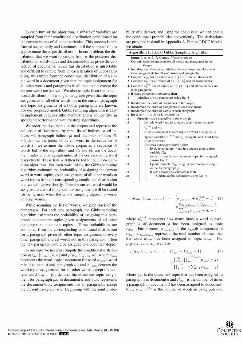
In each turn of the algorithm, a subset of variables aresampled from their conditional distribution conditioned onthe current values of all other variables. This process is per-formed sequentially and continues until the sampled valuesapproximate the target distribution. In our problem, the dis-tribution that we want to sample from is the posterior dis-tribution of word-topics and document-topics given the col-lection of documents. Since this distribution is intractableand difficult to sample from, in each iteration of Gibbs sam-pling, we sample from the conditional distribution of a sin-gle word in a document given that the topic assignment forall other words and paragraphs in all documents except thecurrent word are known. We also sample from the condi-tional distribution of a single paragraph given that the topicassignments of all other words not in the current paragraphand topic assignments of all other paragraphs are known.For our proposed model, Gibbs sampling algorithm is easyto implement, requires little memory, and is competitive inspeed and performance with existing algorithms.

We order the documents in the corpus and represent thecollection of documents by three list of indices: word in-dices wl, paragraph indices pl and document indices dl.wli denotes the index of the ith word in the sequence ofwords (if we assume the whole corpus as a sequence ofwords fed to the algorithm) and dli and pli are the docu-ment index and paragraph index of the corresponding wordrespectively. These lists will then be fed to the Gibbs Sam-pling algorithm. For each word token, the Gibbs samplingalgorithm estimates the probability of assigning the currentword to word-topics given assignment of all other words toword-topics from the corresponding conditional distributionthat we will derive shortly. Then the current word would beassigned to a word-topic and this assignment will be storedfor being used when the Gibbs sampling algorithm workson other words.

While scanning the list of words, we keep track of theparagraphs. For each new paragraph, the Gibbs samplingalgorithm estimates the probability of assigning this para-graph to document-topics given assignments of all otherparagraphs to document-topics. These probabilities arecomputed from the corresponding conditional distributionfor a paragraph given all other topic assignment to everyother paragraph and all words not in this paragraph. Thenthe new paragraph would be assigned to a document-topic.

In our case we need to compute the conditional distribu-tion p(zdsn|z−dsn, y, w) and p(yds|z, y−ds, w), where zdsn

represents the word-topic assignment for word wdsn ( wordn in document d and paragraph s ) and z−dsn denotes theword-topic assignments for all other words except the cur-rent word wdsn. yds denotes the document-topic assign-ment for paragraph pds in document d and y−ds representsthe document-topic assignments for all paragraphs exceptthe current paragraph pds. Beginning with the joint proba-

bility of a dataset, and using the chain rule, we can obtainthe conditional probabilities conveniently. The derivationsare provided in detail in Appendix A. For the LDCC Model,we obtain:

Algorithm 1: LDCC Gibbs Sampling AlgorithmInput: δ, α, η, L, K,Corpus, MaxIterationOutput: topic assignments for all words and paragraphs in the

CorpusInitialization: Randomly, initialize the word-topic and document1topic assignments for all word token and paragraphsCompute Pdk for all values of k ∈ {1..K} and all documents2Compute nlv for all values of l ∈ {1..L} and all word tokens3

Compute n(ds)l

for all values of l ∈ {1..L} and all documents and4their paragraphsif doing parameter estimation then5

Initialize alpha parameters using Eq. 46

Randomize the order of documents in the corpus7Randomize the order of paragraphs in each document8Randomize the order of words in each paragraph9for iter ← 1 to MaxIteration do10

foreach word i according to the order do11Exclude word i and its assigned topic l from variables12

n(ds)l

and nli

newl = sample new word-topic for word i using Eq. 213

Update variables n(ds)l

and nli using the new word-topic14newl for word iif entered a new paragraph j then15

Exclude paragraph j and its assigned topic k from16variable Pdk

newk = sample new document-topic for paragraph17j using Eq. 3Update variable Pdk using the new document-topic18newk for paragraph jif doing parameter estimation then19

Update alpha parameters using Eqs. 420

p(zdsn|z−dsn, y, w) = (αydszdsn+ n(ds)

zdsn− 1) (2)

×nzdsnwdsn+ ηwdsn

− 1∑Vv=1 nzdsnv + ηv − 1

where n(ds)zdsn represents how many times a word in para-

graph s of document d has been assigned to topiczdsn. Furthermore, αydszdsn

is the zdsnth component inαyds

. nzdsnwdsnrepresents the total number of times that

the word wdsn has been assigned to topic zdsn. Forp(yds|z, y−ds, w), we have

p(yds|z, y−ds, w) = (δyds+ Pdyds

− 1) (3)

×∏L

l=1

∏n(ds)l

−1

j=0 (αydsl + j)∏n(ds)−1j=0 (

∑Ll=1 αydsl + j)

where yds is the document-topic that has been assigned toparagraph s in document d and Pdyds

is the number of timesa paragraph in document d has been assigned to document-topic yds. n(ds) is the number of words in paragraph s of

Proceedings of the Sixth International Conference on Data Mining (ICDM'06)0-7695-2701-9/06 $20.00 © 2006

SYMBOL DESCRIPTIONL number of word-topicsK number of document-topicsNs number of words in paragraph sM number of documents in the collectiony document-topic variable for the corpusz word-topic variable for the corpusδ parameters of the Dirichlet prior on document-topicsα matrix of K × L dimensions, row i represents

mixing proportion of word-topics in document-topic iβ parameters of multinomial distribution of words

conditioned on word-topicsη parameters of the prior probability for distribution

of words conditioned on word-topicsφ mixing proportion of document-topics in documentθs mixing proportion of word-topics in the text segment swdsn word n in paragraph s of document dzdsn word-topic assignment for word wdsn

z−dsn word-topic assignments for all other words exceptthe current word wdsn

nlv number of times that the word v assigned to topic l

n(ds)l

number of times a word in paragraph s of document dassigned to topic l

yds document-topic assigned to paragraph s in document dPdk number of paragraphs in document d assigned to

document-topic k

n(ds) number of words in paragraph s of document d

Table 1. List of symbols used in this paper

document d. δydsis the corresponding Dirichlet parameter

for document-topic yds that the paragraph s in document dhas been assigned to.

The Gibbs sampling algorithm is initialized by assigningeach word token to a random word-topic in [1..L] and eachparagraph to random document-topic [1..K]. A number ofinitial samples have to be discarded (also known as burn-insamples) because they are poor estimates of the posterior.After this burn-in period, the next Gibbs samples start toapproximate the target distribution (i.e., the posterior distri-bution over word-topic and document-topic assignments).Now, we pick a number of Gibbs samples and save them asa representative set of samples from this distribution. Thisshould be done at regularly spaced intervals to prevent cor-relations between samples [9].

In the LDA model as adopted by previous works, theDirichlet parameters α are assumed to be given and fixed.This would give us reasonable results when we choose auniform Dirichlet. But for our proposed model, the pa-rameters α capture relationships between document andword topics and must be learned from the data. In asense, they somehow summarize the corresponding term-document matrix of the corpus. For estimating parametersof a Dirichlet distribution, one can use different approachesproposed in the literature [17]. These methods are based onmaximum likelihood or maximum a posteriori estimationof parameters. There is no closed-form solution for thesemethods and one should use iterative methods to learn theparameters. In order to avoid these often computationally

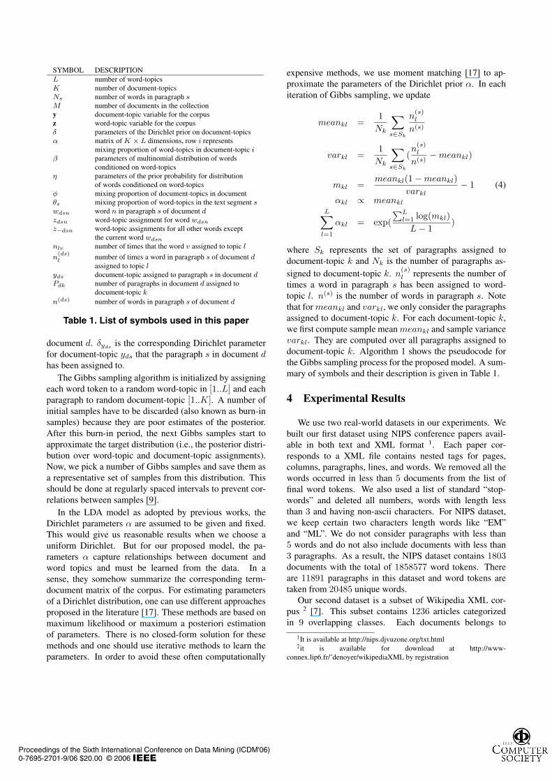
expensive methods, we use moment matching [17] to ap-proximate the parameters of the Dirichlet prior α. In eachiteration of Gibbs sampling, we update

meankl =1

Nk

∑s∈Sk

n(s)l

n(s)

varkl =1

Nk

∑s∈Sk

(n

(s)l

n(s)− meankl)

mkl =meankl(1 − meankl)

varkl− 1 (4)

αkl ∝ meankl

L∑l=1

αkl = exp(∑L

l=1 log(mkl)L − 1

)

where Sk represents the set of paragraphs assigned todocument-topic k and Nk is the number of paragraphs as-signed to document-topic k. n

(s)l represents the number of

times a word in paragraph s has been assigned to word-topic l. n(s) is the number of words in paragraph s. Notethat for meankl and varkl, we only consider the paragraphsassigned to document-topic k. For each document-topic k,we first compute sample mean meankl and sample variancevarkl. They are computed over all paragraphs assigned todocument-topic k. Algorithm 1 shows the pseudocode forthe Gibbs sampling process for the proposed model. A sum-mary of symbols and their description is given in Table 1.

4 Experimental Results

We use two real-world datasets in our experiments. Webuilt our first dataset using NIPS conference papers avail-able in both text and XML format 1. Each paper cor-responds to a XML file contains nested tags for pages,columns, paragraphs, lines, and words. We removed all thewords occurred in less than 5 documents from the list offinal word tokens. We also used a list of standard “stop-words” and deleted all numbers, words with length lessthan 3 and having non-ascii characters. For NIPS dataset,we keep certain two characters length words like “EM”and “ML”. We do not consider paragraphs with less than5 words and do not also include documents with less than3 paragraphs. As a result, the NIPS dataset contains 1803documents with the total of 1858577 word tokens. Thereare 11891 paragraphs in this dataset and word tokens aretaken from 20485 unique words.

Our second dataset is a subset of Wikipedia XML cor-pus 2 [7]. This subset contains 1236 articles categorizedin 9 overlapping classes. Each documents belongs to

1It is available at http://nips.djvuzone.org/txt.html2it is available for download at http://www-

connex.lip6.fr/˜denoyer/wikipediaXML by registration

Proceedings of the Sixth International Conference on Data Mining (ICDM'06)0-7695-2701-9/06 $20.00 © 2006

topic 1 topic 2 topic 3 topic 4 topic 5 topic 6 topic 7 topic 8 topic 9

error neuron image analog data control function rule distributiongeneralization neurons images circuit clustering model functions rules probabilitylearning synaptic object current principal motor basis set gaussiantraining firing recognition figure cluster forward linear step dataoptimal spike face chip pca inverse regression form parametersorder time objects voltage set dynamics kernel fuzzy modellarge activity hand vlsi algorithm controller space problem bayesianaverage rate pixel circuits points feedback gaussian relative mixturesmall synapses system digital approach system approximation extraction densityexamples potential view implementation clusters position rbf expert likelihood

Figure 2. Example word-topics for the NIPS datasettopic 1 topic 2 topic 3 topic 4 topic 5 topic 6 topic 7 topic 8 topic 9 topic 10

language game church house air league war apollo party systemenglish player god parliament aircraft football german earth government computergreek cards christian members world team army moon president gamelanguages players jesus commons force world soviet lunar political gamesword games christ lords military club battle time national applerussell play orthodox bill ship home germany mission minister ataricentury card baptism act gun season world program states commodoretheory hand life power war won forces module united homewords round catholic chopin ships game french jpg election softwaremodern played roman speaker navy major union crew state video

Figure 3. Example word-topics for the Wikipedia dataset

1.47 classes on average. The biggest class corresponds to”Art/Categories“ whit 510 documents. The smallest class,”United Kingdom/Categories“ has 74 documents. There are774958 word tokens, 21453 paragraphs and 17406 uniquewords after preprocessing. The preprocessing phase is sim-ilar to the one for NIPS dataset. For the Wikipedia dataset,we do not have the tags for separating words, therefore weused all delimiting characters to separate words.

In this section, we describe the details of our experimentsthat demonstrate the improved performance of LDCC onNIPS dataset, compared to the LDA in terms of generaliza-tion of the topics found measured by perplexity. We alsoshow the improved clustering performance of LDCC com-pared to the MOC and MOCC models.

In Gibbs sampling for both LDCC and LDA, we run 5markov chains, discarding the first 500 iterations as burn-initerations, and then draw 5 samples from each chain at a lagof 50 iterations, a total of 25 samples for each experiment.For the NIPS dataset, the total training time for LDCC isapproximately 23 hours on a machine with a dual core In-tel Pentium IV 64-bit (EM64T ) processor (2 × 3.0GHzprocessor) with 2GB of RAM.

4.1 Word and Document Topic Examples

In this section, we show 9 word-topics derived fromNIPS dataset and 10 word-topics derived from Wikipediadataset, each represented by their first 10 most probablewords, presented in Fig.2 and Fig.3 respectively. As it canbe seen, the model seems to be able to capture some of theunderlying word-topics in both datasets.

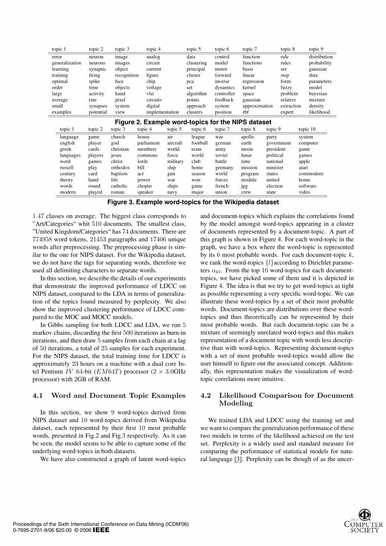
We have also constructed a graph of latent word-topics

and document-topics which explains the correlations foundby the model amongst word-topics appearing in a clusterof documents represented by a document-topic. A part ofthis graph is shown in Figure 4. For each word-topic in thegraph, we have a box where the word-topic is representedby its 6 most probable words. For each document-topic k,we rank the word-topics {l}according to Dirichlet parame-ters αkl. From the top 10 word-topics for each document-topics, we have picked some of them and it is depicted inFigure 4. The idea is that we try to get word-topics as tightas possible representing a very specific word-topic. We canillustrate these word-topics by a set of their most probablewords. Document-topics are distributions over these word-topics and thus theoretically can be represented by theirmost probable words. But each document-topic can be amixture of seemingly unrelated word-topics and this makesrepresentation of a document-topic with words less descrip-tive than with word-topics. Representing document-topicswith a set of most probable word-topics would allow theuser himself to figure out the associated concept. Addition-ally, this representation makes the visualization of word-topic correlations more intuitive.

4.2 Likelihood Comparison for DocumentModeling

We trained LDA and LDCC using the training set andwe want to compare the generalization performance of thesetwo models in terms of the likelihood achieved on the testset. Perplexity is a widely used and standard measure forcomparing the performance of statistical models for natu-ral language [3]. Perplexity can be though of as the uncer-

Proceedings of the Sixth International Conference on Data Mining (ICDM'06)0-7695-2701-9/06 $20.00 © 2006

distributionprobabilityGaussianparametersBayesianmixture

timesequencetemporalPredictionDelaySeries

Sequence

linearnonlinearanalysissingleInputOrder

StateOptimalTimePolicyAction

ReinforcementFunction

ComponentIndependentAnalysisIca

SourceData

Channel

AuditorySoundTarget

LocalizationSpectralCorrelation

AnalogCircuitCurrentChipVoltageVlsi

RuleSetStepFuzzy

ExtractionExpert

RegionHumanChainMousePrecursorReceptor

NeuronSynapticFiringSpikeTimeActivity

ResultsSimilarLocalSmall

ExperimentsShow

WeightFunctionGradientEquationLearningAlgorithm

AlgorithmProblemMethodNumberSolutionSearch

Figure 4. Correlation identified by LDCC between word-topics. Each circle shows a document-topicand each box corresponds to a word-topic. As it can be seen, one document-topic can be connectedto several word-topics and capture their correlation.

tainty in predicting a single word according to the modeland lower values are better. Formally, for a test set of Mdocuments, it is defined as:

perplexity(Dtest) = exp

(−∑M

d=1 log p(wd)∑Md=1 Nd

)(5)

In order to compute perplexity, we need to compute the like-lihood p(w) and this requires summing over all possible as-signments of words to word topics z and text segments (inour datasets, the text segments corresponds to paragraphs)to document topics y. This problem has no closed-form so-lution. Previous work on LDA [10] has used harmonic meanestimator introduced in [18]. We estimate p(w) by takingthe harmonic mean of a set of values p(w|z). By using thechain rule and integrating the parameter out, we get:

p(w|z) =

(Γ(∑V

v=1 ηv)∏Vv=1 Γ(ηv)

)L L∏l=1

∏Vv=1 Γ(nlv + ηv)

Γ(∑V

v=1 nlv + ηv)(6)

z is sampled from the posterior P (z|w) using the Gibbssampling procedure described in section 3. The derivationof this is similar to the one described in Appendix A.

In these experiments, we use the NIPS dataset and splitit into 80% for training and 20% for calculating the likeli-hood. We use 20 document topics and change the number ofword topics from 20 to 100. We split the dataset randomlyso that the training and test subsets have relatively 80% and20% of the documents respectively and each topic in bothsubsets has at least 5 documents.

We present perplexity results for different number ofword topics in Fig. 5. For all these experiments, the num-ber of document topics are assumed fixed and equal to 20.As it can be observed, for different number of word-topics,

2000

4000

6000

8000

10000

12000

14000

0 20 40 60 80 100 120Number of Word Topics

Perp

lexi

tyLDA LDCC

Figure 5. Perplexity results for NIPS datasetwith different numbers of topics

LDCC always produce lower perplexity compared to LDA.As it can be seen in Fig. 5, the perplexity for the LDCCmethod is increasing in the range of values that we haveexamined, as opposed to LDA model. This shows that theproposed method can not keep up its generalization perfor-mance as the number of word-topics increases, in contrastto the LDA model.

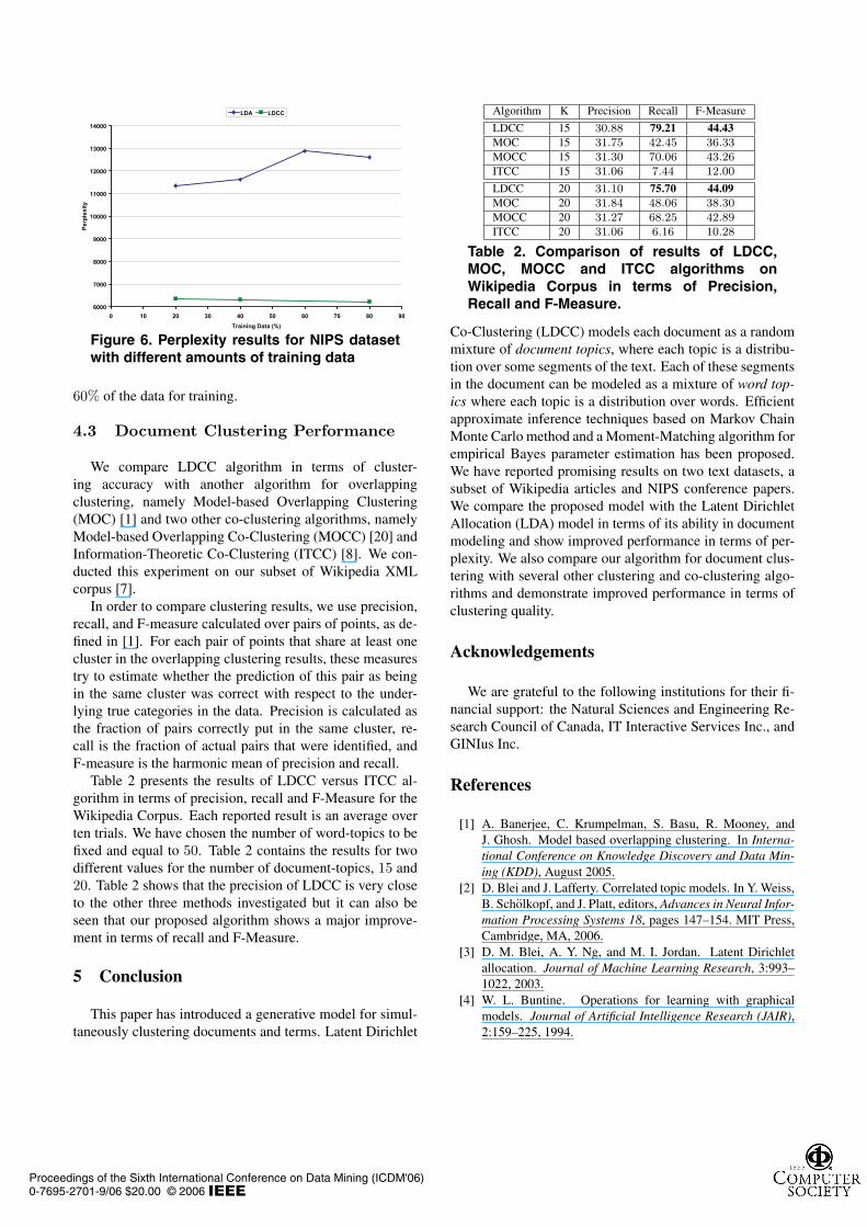
We also show the results comparing LDCC and LDAwhen we use different amount of training data for learningthe model parameters. In these set of experiments, the num-ber of word-topics and document-topics are assumed fixedand equal to 20 and 100 respectively. We present these re-sults in Fig. 6. As it can be seen, the LDCC model haslower perplexity compared to LDA model as the amount oftraining data increase. The perplexity for LDCC model de-creases while we increase the amount of training data whilefor the LDA model, the perplexity has a peak when we use

Proceedings of the Sixth International Conference on Data Mining (ICDM'06)0-7695-2701-9/06 $20.00 © 2006

6000

7000

8000

9000

10000

11000

12000

13000

14000

0 10 20 30 40 50 60 70 80 90Training Data (%)

Perp

lexi

ty

LDA LDCC

Figure 6. Perplexity results for NIPS datasetwith different amounts of training data

60% of the data for training.

4.3 Document Clustering Performance

We compare LDCC algorithm in terms of cluster-ing accuracy with another algorithm for overlappingclustering, namely Model-based Overlapping Clustering(MOC) [1] and two other co-clustering algorithms, namelyModel-based Overlapping Co-Clustering (MOCC) [20] andInformation-Theoretic Co-Clustering (ITCC) [8]. We con-ducted this experiment on our subset of Wikipedia XMLcorpus [7].

In order to compare clustering results, we use precision,recall, and F-measure calculated over pairs of points, as de-fined in [1]. For each pair of points that share at least onecluster in the overlapping clustering results, these measurestry to estimate whether the prediction of this pair as beingin the same cluster was correct with respect to the under-lying true categories in the data. Precision is calculated asthe fraction of pairs correctly put in the same cluster, re-call is the fraction of actual pairs that were identified, andF-measure is the harmonic mean of precision and recall.

Table 2 presents the results of LDCC versus ITCC al-gorithm in terms of precision, recall and F-Measure for theWikipedia Corpus. Each reported result is an average overten trials. We have chosen the number of word-topics to befixed and equal to 50. Table 2 contains the results for twodifferent values for the number of document-topics, 15 and20. Table 2 shows that the precision of LDCC is very closeto the other three methods investigated but it can also beseen that our proposed algorithm shows a major improve-ment in terms of recall and F-Measure.

5 Conclusion

This paper has introduced a generative model for simul-taneously clustering documents and terms. Latent Dirichlet

Algorithm K Precision Recall F-Measure

LDCC 15 30.88 79.21 44.43MOC 15 31.75 42.45 36.33MOCC 15 31.30 70.06 43.26ITCC 15 31.06 7.44 12.00

LDCC 20 31.10 75.70 44.09MOC 20 31.84 48.06 38.30MOCC 20 31.27 68.25 42.89ITCC 20 31.06 6.16 10.28

Table 2. Comparison of results of LDCC,MOC, MOCC and ITCC algorithms onWikipedia Corpus in terms of Precision,Recall and F-Measure.

Co-Clustering (LDCC) models each document as a randommixture of document topics, where each topic is a distribu-tion over some segments of the text. Each of these segmentsin the document can be modeled as a mixture of word top-ics where each topic is a distribution over words. Efficientapproximate inference techniques based on Markov ChainMonte Carlo method and a Moment-Matching algorithm forempirical Bayes parameter estimation has been proposed.We have reported promising results on two text datasets, asubset of Wikipedia articles and NIPS conference papers.We compare the proposed model with the Latent DirichletAllocation (LDA) model in terms of its ability in documentmodeling and show improved performance in terms of per-plexity. We also compare our algorithm for document clus-tering with several other clustering and co-clustering algo-rithms and demonstrate improved performance in terms ofclustering quality.

Acknowledgements

We are grateful to the following institutions for their fi-nancial support: the Natural Sciences and Engineering Re-search Council of Canada, IT Interactive Services Inc., andGINIus Inc.

References

[1] A. Banerjee, C. Krumpelman, S. Basu, R. Mooney, andJ. Ghosh. Model based overlapping clustering. In Interna-tional Conference on Knowledge Discovery and Data Min-ing (KDD), August 2005.

[2] D. Blei and J. Lafferty. Correlated topic models. In Y. Weiss,B. Scholkopf, and J. Platt, editors, Advances in Neural Infor-mation Processing Systems 18, pages 147–154. MIT Press,Cambridge, MA, 2006.

[3] D. M. Blei, A. Y. Ng, and M. I. Jordan. Latent Dirichletallocation. Journal of Machine Learning Research, 3:993–1022, 2003.

[4] W. L. Buntine. Operations for learning with graphicalmodels. Journal of Artificial Intelligence Research (JAIR),2:159–225, 1994.

Proceedings of the Sixth International Conference on Data Mining (ICDM'06)0-7695-2701-9/06 $20.00 © 2006

[5] H. Chipman and H. Gu. Interpretable dimension reduc-tion. Journal of Applied Statistics, 32(9):969–987, Novem-ber 2005.

[6] S. C. Deerwester, S. T. Dumais, T. K. Landauer, G. W. Fur-nas, and R. A. Harshman. Indexing by latent semantic analy-sis. Journal of the American Society of Information Science,41(6):391–407, 1990.

[7] L. Denoyer and P. Gallinari. The Wikipedia XML Corpus.SIGIR Forum, 2006. Last accessed, June 2006.

[8] I. S. Dhillon, S. Mallela, and D. S. Modha. Information-theoretic co-clustering. In KDD ’03: Proceedings of theninth ACM SIGKDD International Conference on Knowl-edge Discovery and Data Mining, pages 89–98, New York,NY, USA, 2003. ACM Press.

[9] W. R. Gilks. Markov Chain Monte Carlo in Practice. Chap-man & Hall/CRC, December 1995.

[10] T. L. Griffiths and M. Steyvers. Finding scientific top-ics. Proceedings of the National Academy of Sciences, 101Suppl 1:5228–5235, April 2004.

[11] T. L. Griffiths, M. Steyvers, D. M. Blei, and J. B. Tenen-baum. Integrating topics and syntax. In L. K. Saul, Y. Weiss,and L. Bottou, editors, Advances in Neural Information Pro-cessing Systems 17, pages 537–544. MIT Press, Cambridge,MA, 2005.

[12] T. Hofmann. Probabilistic latent semantic indexing. InSIGIR ’99: Proceedings of the 22nd Annual InternationalACM SIGIR Conference on Research and Development inInformation Retrieval, pages 50–57, New York, NY, USA,1999. ACM Press.

[13] M. Keller and S. Bengio. Theme Topic Mixture Model:A Graphical Model for Document Representation. IDIAP-RR 05, IDIAP, 2004.

[14] W. Li and A. Mccallum. Pachinko allocation: Dag-structured mixture models of topic correlations. In ICML’06: 23rd International Conference on Machine Learning,Pittsburgh, Pennsylvania, USA, June 2006.

[15] S. C. Madeira and A. L. Oliveira. Biclustering algo-rithms for biological data analysis: A survey. IEEE/ACMTransactions on Computational Biology and Bioinformatics(TCBB), 1(1):24–45, 2004.

[16] T. Minka and J. Laferty. Expectation-propagation for thegenerative aspect model, 2002.

[17] T. P. Minka. Estimating a Dirichlet distribution. Technicalreport, MIT, 2000.

[18] M. Newton and A. Raftery. Approximate Bayesian inferencewith the weighted likelihood bootstrap. Journal of the RoyalStatistical Society. Series B, 56:3–48, 1994.

[19] F. Sebastiani. Machine learning in automated text catego-rization. ACM Computing Surveys, 34(1):1–47, 2002.

[20] M. Shafiei and E. Milios. Model-based overlapping co-clustering. In Proceedings of the Fourth Workshop on TextMining, Sixth SIAM International Conference on Data Min-ing, Bethesda, Maryland, April 22 2006.

[21] M. Steyvers and T. Griffiths. Probabilistic topic models. InT. Landauer, D. Mcnamara, S. Dennis, and W. Kintsch, ed-itors, Latent Semantic Analysis: A Road to Meaning. Lau-rence Erlbaum, 2005.

[22] Y. W. Teh, M. I. Jordan, M. J. Beal, and D. M. Blei. Hierar-chical Dirichlet processes. Journal of the American Statisti-cal Association, 2006.

A Gibbs Sampling Derivations

Beginning with the joint distribution p(w, z, y), we cantake advantage of conjugate priors to simplify the formulae.All symbols are defined in Section 3 and Table 1.

p(w, z, y) = p(w|z, η)p(z|α, y)p(y|δ)

=

∫p(w|z, β)p(β|η)dβ

∫p(z|θ)p(θ|α, y)dθ

∫p(y|φ)p(φ|δ)dφ

=

∫ M∏d=1

Sd∏s=1

Nsd∏n=1

p(wzdsn |βzdsn )

L∏l=1

p(βl|η)dβ

∫ M∏d=1

Sd∏s=1

(Nsd∏n=1

p(zdsn|θds)p(θds|α, yds)

)dθ

∫ M∏d=1

(Sd∏

s=1

p(yds|φd)p(φd|δ))

dφ

=

∫ L∏l=1

V∏v=1

βnlvlv

L∏l=1

(Γ(∑V

v=1ηv)∏V

v=1Γ(ηv)

V∏v=1

βηv−1lv

)dβ

∫ M∏d=1

Sd∏s=1

L∏l=1

θn(ds)l

dsl

M∏d=1

Sd∏s=1

(Γ(∑L

l=1αydsl)∏L

l=1Γ(αydsl)

L∏l=1

θαydsl−1

dsl

)dθ

∫ M∏d=1

K∏k=1

φPdkdk

M∏d=1

(Γ(∑K

k=1δk)∏K

k=1Γ(δk)

K∏k=1

φδk−1dk

)dφ

=

(Γ(∑V

v=1ηv)∏V

v=1Γ(ηv)

)L L∏l=1

∏V

v=1Γ(nlv + ηv)

Γ(∑V

v=1nlv + ηv)

M∏d=1

Sd∏s=1

(Γ(∑L

l=1αydsl)∏L

l=1Γ(αydsl)

)M∏

d=1

Sd∏s=1

∏L

l=1Γ(αydsl + n

(ds)l

)

Γ(∑L

l=1αydsl + n

(ds)l

)(Γ(∑K

k=1δk)∏K

k=1Γ(δk)

)M M∏d=1

∏K

k=1Γ(δk + Pdk)

Γ(∑K

k=1δk + Pdk)

Using the chain rule, we have

p(zdsn|z−dsn, y, w) =p(zdsn, wdsn|z−dsn, y, w−dsn)

p(wdsn|z−dsn, y, w−dsn)

∝ p(z,y,w)p(z−dsn,y,w−dsn)

= (αydszdsn + n(ds)zdsn

− 1)× nzdsnwdsn+ηwdsn

−1∑V

v=1nzdsnv+ηv−1

Using chain rule, again we have

p(yds|z, y−ds, w) =p(zds, yds, wds|z−ds, y−ds, w−ds)

p(wds, zds|z−ds, y−ds, w−ds)

∝ p(z,y,w)p(z−ds,y−ds,w−ds)

= (δyds + Pdyds− 1)× Γ(

∑L

l=1αydsl)∏L

l=1Γ(αydsl)

∏L

l=1Γ(αydsl+n

(ds)l

)

Γ(∑L

l=1αydsl+n

(ds)l

)

= (δyds + Pdyds− 1)×

∏L

l=1

∏n(ds)l

−1

j=0 (αydsl+j)∏n(ds)−1

j=0(∑L

l=1αydsl+j)

Proceedings of the Sixth International Conference on Data Mining (ICDM'06)0-7695-2701-9/06 $20.00 © 2006