Embed Size (px)
Citation preview
The Construction of Labeled Line Drawings from Intensity
Images1
Deborah Anne TryttenSchool of Computer ScienceUniversity of Oklahoma
Norman, OK 73019-0631, [email protected]
Fax: 405-325-4044
Mihran TuceryanEuropean Computer-Industry Research Centre (ECRC)
Arabellastra�e 1781925 M�unchen, Germany
Fax: +(49)(89) 92699-170
June 27, 1994
1This research was supported in part by the National Science Foundation grants IRI-9103143 and CDA-
8806599. The facilities of the Pattern Recognition and Image Processing Laboratory at the Michigan
State University are also gratefully acknowledged.
Abstract
This paper describes the POLL (Perceptual Organization and Line Labeling) system for
obtaining labeled line drawings from single intensity images using an integrated blackboard
system. This system emphasizes the data driven extraction of 3D geometric information from
intensity images. The robustness of the system comes from it being implemented in an integrated
framework in which the errors made by one module can be diagnosed and corrected by the
constraints imposed by other modules. The system is able to generate an initial line drawing
from an intensity image in the domain of piecewise smooth objects.
Four modules were used as knowledge sources: weak membrane edge detection, curvilinear
grouping, proximity grouping, and curvilinear line labeling. An initial representation of the
image data is built using the �rst three knowledge sources. This representation is analyzed
using a modi�ed curvilinear line labeling algorithm developed in this paper that uses �gure{
ground separation to constrain legal line labelings. This modi�ed line labeling algorithm can
diagnose problems with the initial representation. The modi�ed line labeling algorithm can
�nd errors such as missing edges, improperly typed vertices, and missing phantom junctions.
Errors in the representation can be �xed using a set of heuristics that were created to repair
common mistakes. If no irreparable errors are found in the representation, then the modi�ed
line labeling algorithm produces a 3D interpretation of the data in the input image without
explicitly reconstructing 3D shape.
1 Introduction
One of the main goals of computer vision is to extract spatial and geometric information about
the external world seen in an image. The extracted spatial information could be as simple
as identifying empty spaces for navigational or obstacle avoidance purposes, or it could be for
manipulation or object recognition purposes.
Object recognition is one of the most important and frequently researched topics in compu-
tational vision, due to its potential for wide applicability to important automation problems.
There are many proposed methods in the literature for accomplishing object recognition. One
very common approach is to match a representation of an object that was derived from image
data to 3D descriptions of objects stored in a model database. Such 3D descriptions can also
be used for purposes other than recognition, such as manipulation.
In an intensity image, the light received by the camera is a function of several factors such
as the shape and re ective properties of the surfaces, the number, type, and relative direction
of light sources, and the viewing direction. These factors are highly interrelated making the
direct recovery of the 3D shape of the imaged objects diÆcult. Therefore, the extraction of a
3D description from an image involves an inference process. There is a broad literature on a set
of techniques for inferring such information based on explicit reconstruction of the 3D shape.
These include shape from shading [1, 2, 3, 4], shape from texture [5, 6, 7, 8], shape from motion
[9], shape from stereo [10, 11], and many other similar processes collectively referred to as \shape
from X." While these algorithms are gaining mathematical rigor [9], they still lack the robustness
that is necessary to be useful in a general environment. Other approaches include extraction of
qualitative 3D information from images. An early example of such a process is extracting line
drawings from images with possible 3D intrepretations attached. This is attractive because it is
boundary based and terse. Boundaries have been shown to be useful in human vision [12]. The
problem is that it is diÆcult to reliably extract the perfect line drawings from images which are
necessary for most line labeling algorithms to work properly.
Another approach to extracting qualitative information from images involves inferring struc-
ture through perceptual organization. This line of research has been motivated by cues from the
human visual system [13]. The human visual system can organize and interpret images even
when 3D shape cannot be reconstructed. To do this, the salient features of the image, called
tokens, need to be identi�ed, organized, and interpreted. The capability of the human visual
system to group tokens together in a meaningful way without any prior knowledge of the con-
tents of the image, is called perceptual organization. Perceptual organization collects tokens in
the image plane together into signi�cant groupings using only general rules. These tokens can be
1
recursively grouped, or subdivided as the scene is further organized. Cooperating and competing
groupings are explored until a globally good organization of the image is found. Groupings of
tokens can then be used to infer 3D properties [14]. The problem with this approach is that of-
ten there are many competing plausible groupings. Deciding among these competing groupings
without the proper 3D context is diÆcult.
This paper will describe the development of the POLL system (Perceptual Organization for
Line Labeling) which uses the processes described above in an integrated manner, to �nd labeled
line drawings from single monochromatic intensity images. Our motivation was:
� to reduce the fragility of each of these individual processes through the use of multiple
cooperative processes which complement each other, and
� to minimize the need for human intervention in this processing
The organization of the paper is as follows. Section 2 will give a brief review of the background
and previous work. Section 3 will describe the overall architecture of the POLL system. Section 4
will explain how the initial analysis of image information is performed with the perceptual
knowledge sources. Section 5 will give the method proposed to discern images that have been
properly analyzed by the initial processing from those that have not using the diagnostic and
interpretive knowledge source. Once inconsistencies in the initial representation of the image
have been found, Section 6 shows how some of these defects can be corrected using the control
and repair knowledge sources. Section 7 will present experimental results. The �nal section,
Section 8, will list the contributions of the paper and suggest related topics for further research.
2 Background
The POLL system's goal is to extract labeled line drawings from intensity images in an integrated
framework. The modules used in the implementation of the POLL system are (a) low level
modules, (b) perceptual organization modules, and (c) a 3D interpretation module in the form
of line labeling. We �rst give a brief review of previous work done which is relevant to the
components of the POLL system.
The low level processing component entails the processes that operate directly on the image
and produce results in the image domain. It includes such modules as edge detection, segmen-
tation, corner detection, etc. There has been a great amount of research done in the individual
modules of this level and there is a vast literature about it. The interested reader can refer to
any standard vision textbook [15, 16].
2
Another module which is integral to the operation of POLL is the perceptual grouping
module. Perceptual grouping is the organization by the human visual system of image tokens in
a scene into meaningful groupings without using any domain speci�c knowledge or without any
explicit shape information being present. An appreciation for this aspect of the human visual
system dates back to the Gestalt school of psychology [17], which identi�ed the �rst principles
of what is now known as perceptual organization. These principles include proximity, similarity,
good continuity, closure, symmetry, and �gure-ground separation.
In computational vision, the importance of perceptual organization was brought to the fore-
front by Witkin and Tenenbaum [18] and Lowe [14]. Witkin and Tenenbaum analyzed the
importance of structure, meaning spatiotemporal coherence or regularity, in visual perception.
They argued that when regular structure is observed, it is signi�cant because it would have been
unlikely to have arisen accidentally. Lowe sharpened this idea in [14] when he proposed that the
signi�cance of a grouping of tokens is proportional to how unlikely the relationship between the
tokens was to have arisen by accident, called non-accidentalness. Other studies that attempt
to model perceptual organization principles computationally include Tuceryan [19], Rosin and
West [20], Trytten [21], McCa�erty [22], Sarkar and Boyer [23], and Mohan and Nevatia [24].
Labeling of line drawings was originally done in the trihedral world [25, 26], and later ex-
tended to general polyhedra [27]. Shadow edges and surface markings were added in [28], and
origami objects were used in [29]. A junction catalog for piecewise smooth objects was derived
by Malik in [30]. Piecewise smooth objects di�er from polyhedra in that the surfaces can be
curved and are not restricted to be planar. There have been various attempts in the past at
extracting labeled line drawings from real images with varying levels of generality and varying
degrees of success [31, 32, 33, 34, 35].
Another major aspect of the POLL system is the integration of various visual processing
modules. Integration has become an important research topic in computational vision [36, 37,
38, 39, 40, 35]. The primary goal of integration is improving the robustness and exibility of
computational vision algorithms.
Moravec's certainty grid [39], Gibbs distribution and Markov Random Field frameworks
(MRFs) [41, 38, 36, 22] are examples of integration within a uniform mathematical framework.
In these approaches often some sort of optimization process is involved in the form of maximiz-
ing a posteriori probabilities or minimizing some energy function. When energy minimization
problems are being solved, it is often desirable that the solution found be smooth. Regulariza-
tion theory is the rigorous approach to smoothness as a constraint which have been suggested
and used by various researchers [42, 43, 44].
3
Any integration strategy that does not exhibit the uniformity of the integration strategies
mentioned above will be classi�ed as non-uniform. This approach is often used for integrating
pairs of processes. Many of these schemes take advantage of the strong constraints in the speci�c
domain under consideration. Examples of this approach include works by Ahuja, et al. [45, 6]
and Malik and Maydan [46].
When the number of processes to be integrated becomes large, creating a non-uniform system
is more diÆcult. If this integration is handled informally, chaos can result. A useful structure
for integrating diverse processes which work on a common problem is the blackboard system
[47, 48]. Blackboard systems have previously been used for image processing and computer vision
[37, 49]. Work is also being done on specialized architectures for blackboards, concurrency and
parallelism, and real time blackboard systems [50].
3 The POLL System
This paper will describe the construction of the POLL system (Perceptual Organization and
Line Labeling) that can �nd labeled line drawings from single intensity images. The input into
the system will be a single intensity image of one or more objects in a domain which will be
precisely described shortly. The output from the system will be a line drawing labeled with a 3D
interpretation, and a database of intermediate representations and partial results that may be
useful for further processing. Finding labeled line drawings is a very diÆcult problem, and there
will be some images which are not correctly processed. In these images, it is desirable to obtain
intermediate information that could be used by other processing modules to work towards the
�nal goal of 3D interpretation.
Visual perceptual organization and 3D interpretation do not consist of a single cohesive
process, but rather of a diverse collection of processes working towards the goal of interpreting
images. For these perceptual processes to be able to cooperate and compete to �nd meaningful
relationships within the image, the processes need to be integrated. Integrated processes can
use each others constraints and expertise to guide the search for good groupings.
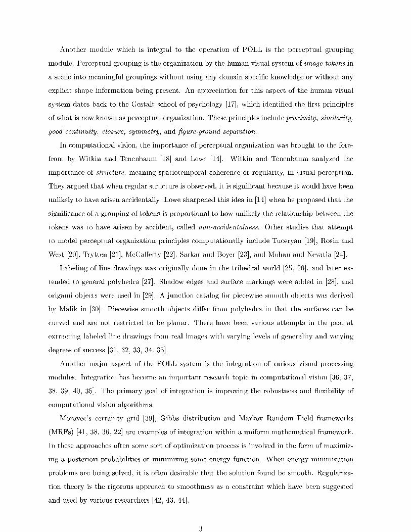
An example of the need for integration is shown in Figure 1. This very simple polyhedral
scene would create enormous diÆculties for existing line labeling methods. The imaged object is
within both the domain of polyhedral objects and the domain of piecewise smooth objects. But
it is unlikely that any edge detection scheme could recover the front corner edge of this object,
since edge detection relies upon spatial variation in intensities and there is no spatial variation
in intensity values across the front edge of the prism. Line labeling modules require perfect
input and cannot recover from edge detection mistakes. And edge detection modules cannot
4
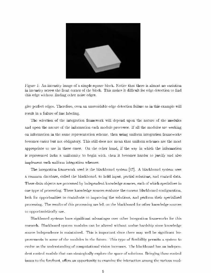
Figure 1: An intensity image of a simple square block. Notice that there is almost no variationin intensity across the front corner of the block. This makes it diÆcult for edge detection to �ndthis edge without �nding other noise edges.
give perfect edges. Therefore, even an unavoidable edge detection failure as in this example will
result in a failure of line labeling.
The selection of the integration framework will depend upon the nature of the modules
and upon the nature of the information each module processes. If all the modules are working
on information in the same representation scheme, then using uniform integration frameworks
becomes easier but not obligatory. This still does not mean that uniform schemes are the most
appropriate to use in these cases. On the other hand, if the way in which the information
is represented lacks a uniformity to begin with, then it becomes harder to justify and also
implement such uniform integration schemes.
The integration framework used is the blackboard system [47]. A blackboard system uses
a common database, called the blackboard, to hold input, partial solutions, and control data.
These data objects are processed by independent knowledge sources, each of which specializes in
one type of processing. These knowledge sources evaluate the current blackboard con�guration,
look for opportunities to contribute to improving the solutions, and perform their specialized
processing. The results of this processing are left on the blackboard for other knowledge sources
to opportunistically use.
Blackboard systems have signi�cant advantages over other integration frameworks for this
research. Blackboard system modules can be altered without undue hardship since knowledge
source independence is maintained. This is important since there may well be signi�cant im-
provements in some of the modules in the future. This type of exibility permits a system to
evolve as the understanding of computational vision increases. The blackboard has an indepen-
dent control module that can strategically explore the space of solutions. Bringing these control
issues to the forefront, o�ers an opportunity to examine the interaction among the various mod-
5
ules. Methods without elaborate control structures cannot provide this type of introspection
into their processing.
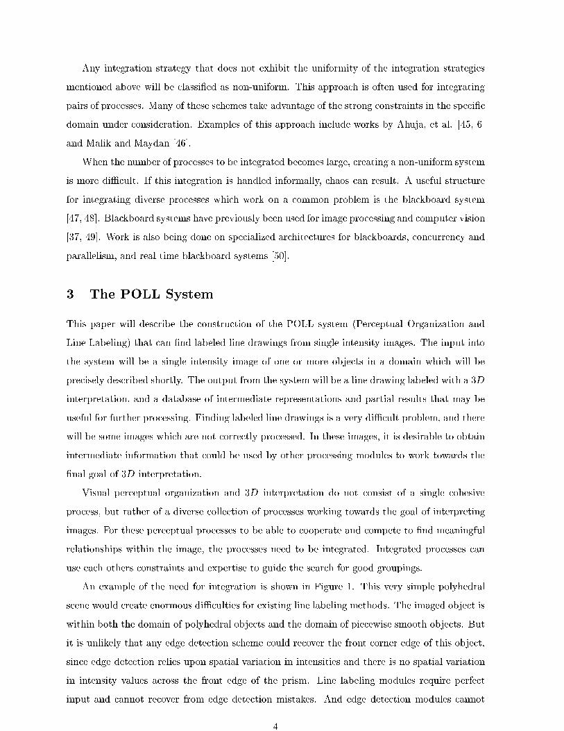
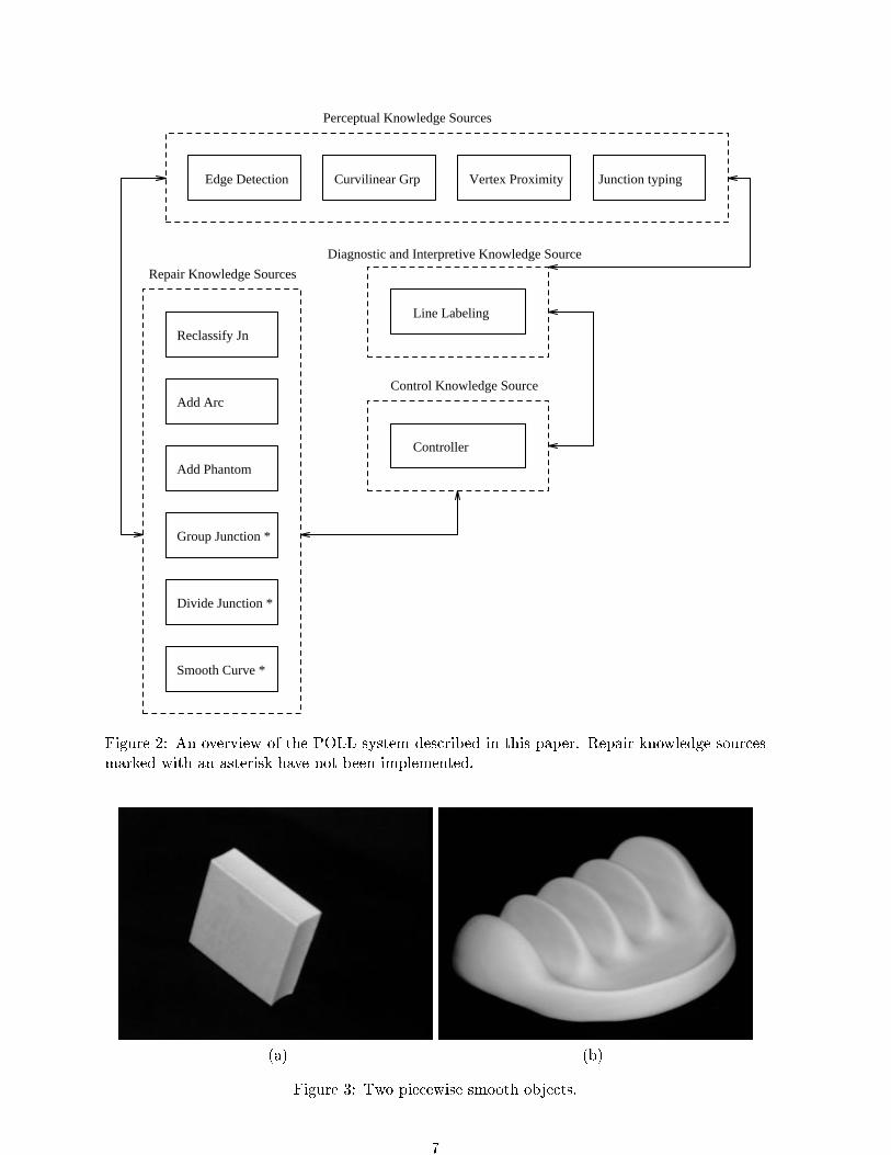
Figure 2 shows the overall structure of the POLL system. The knowledge sources are di-
vided into four groups. The �rst group are the low level (perceptual) knowledge sources. These
knowledge sources bootstrap the initial line drawing using low level processing and perceptual
organization. They are also available to do specialized work for other knowledge sources, and
make other contributions to the blackboard database. The diagnostic and interpretive knowl-
edge source is a modi�ed line labeling paradigm that can examine a line drawing and locate
inconsistencies. If there are no inconsistencies, a 3D interpretation of the line drawing will
be found. The information produced by the diagnostic and interpretive knowledge source is
available for the control knowledge source. This knowledge source selects which of the available
repair strategies, if any, is suitable for �xing problems with the line labeling. The repair knowl-
edge sources are called by the control knowledge source to �x the line labeling, and in turn call
the perceptual knowledge source to reevaluate previous results in light of the the more global
diagnostic information that is available. The integration in this system comes from the fact that
there is interaction, cooperation, and feedback among the various knowledge sources through
communications via the blackboard. Thus, the diagnostic line labeling knowledge source can
have a top-down e�ect on the lower level modules by enforcing constraints in its domain. Notice
also that through this type of interaction, there is no �xed, sequential order of processing which
must be applied to every image. Depending upon the content and complexity of the image, there
may be many di�erent orders of processing and many iterations through the e�ective feedback
loops. This is where the power of integration schemes originates.
The perceptual knowledge sources used in this system are weak membrane edge detection
[51], an algorithm that performs edge grouping on the basis of continuity [21], a module that
analyzes vertex proximity, and a module that can determine the type of line drawing junctions.
A modi�ed line labeling algorithm will be used as the diagnostic and interpretive knowledge
source.
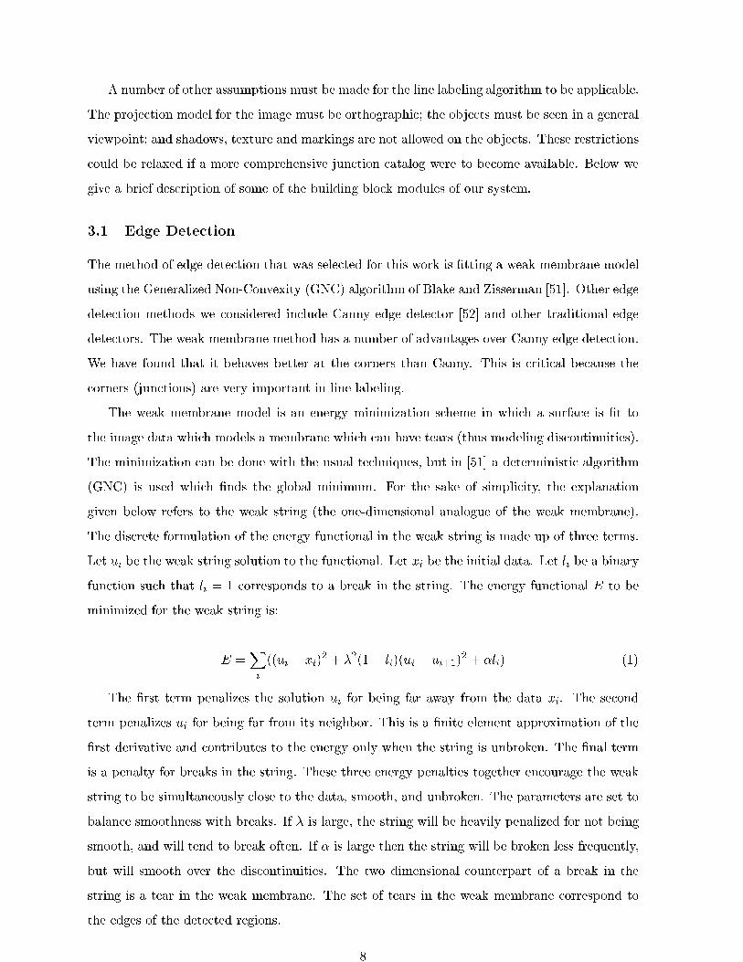
The domain of objects that is used in this paper is the set of piecewise smooth objects
de�ned precisely by Malik in [30]. We restrict this domain, however, in order to help control the
complexity of the object domain: the number of surfaces that can meet at a vertex in an object
in our domain is limited to three. Some examples of real objects that are in the domain and
are correctly processed by the POLL system are shown in Figure 3. Examples of objects that
are not in this domain are wireframe objects, origami objects, objects where more than three
surfaces meet at a junction, a single nappe of a right circular cone.
6
Perceptual Knowledge Sources
Edge Detection Curvilinear Grp Vertex Proximity Junction typing
Line Labeling
Controller
Repair Knowledge Sources
Control Knowledge Source
Reclassify Jn
Add Phantom
Add Arc
Diagnostic and Interpretive Knowledge Source
Group Junction *
Divide Junction *
Smooth Curve *
Figure 2: An overview of the POLL system described in this paper. Repair knowledge sourcesmarked with an asterisk have not been implemented.
(a) (b)
Figure 3: Two piecewise smooth objects.
7
A number of other assumptions must be made for the line labeling algorithm to be applicable.
The projection model for the image must be orthographic; the objects must be seen in a general
viewpoint; and shadows, texture and markings are not allowed on the objects. These restrictions
could be relaxed if a more comprehensive junction catalog were to become available. Below we
give a brief description of some of the building block modules of our system.
3.1 Edge Detection
The method of edge detection that was selected for this work is �tting a weak membrane model
using the Generalized Non-Convexity (GNC) algorithm of Blake and Zisserman [51]. Other edge
detection methods we considered include Canny edge detector [52] and other traditional edge
detectors. The weak membrane method has a number of advantages over Canny edge detection.
We have found that it behaves better at the corners than Canny. This is critical because the
corners (junctions) are very important in line labeling.
The weak membrane model is an energy minimization scheme in which a surface is �t to
the image data which models a membrane which can have tears (thus modeling discontinuities).
The minimization can be done with the usual techniques, but in [51] a deterministic algorithm
(GNC) is used which �nds the global minimum. For the sake of simplicity, the explanation
given below refers to the weak string (the one-dimensional analogue of the weak membrane).
The discrete formulation of the energy functional in the weak string is made up of three terms.
Let ui be the weak string solution to the functional. Let xi be the initial data. Let li be a binary
function such that li = 1 corresponds to a break in the string. The energy functional E to be
minimized for the weak string is:
E =X
i
((ui � xi)2 + �2(1� li)(ui � ui+1)
2 + �li) (1)
The �rst term penalizes the solution ui for being far away from the data xi. The second
term penalizes ui for being far from its neighbor. This is a �nite element approximation of the
�rst derivative and contributes to the energy only when the string is unbroken. The �nal term
is a penalty for breaks in the string. These three energy penalties together encourage the weak
string to be simultaneously close to the data, smooth, and unbroken. The parameters are set to
balance smoothness with breaks. If � is large, the string will be heavily penalized for not being
smooth, and will tend to break often. If � is large then the string will be broken less frequently,
but will smooth over the discontinuities. The two dimensional counterpart of a break in the
string is a tear in the weak membrane. The set of tears in the weak membrane correspond to
the edges of the detected regions.
8
The energy functional needs to be minimized both with respect to ui, and with respect to
li. This problem is not convex and has the potential to get trapped in local minima during
the minimization process. The GNC algorithm is an attempt to avoid this problem in the
weak membrane model. This procedure has been shown to converge to the global minimum
energy for the weak string, the weak membrane, the weak rod, and the weak plate models if the
discontinuities are much further separated than the scale parameter �.
One advantage of selecting GNC for the edge detection module is that it tends to �nd
complete boundaries around regions even though this is not guaranteed. It does a good job
at the corners and junctions. The weak membrane formulation has only two parameters, both
of which have a physical interpretation. These parameters can be changed into another pair
of parameters which corresponds to scale and contrast sensitivity which is meaningful for edge
detection. The parameters were set initially, after experimentation, and were not altered during
the course of processing all the images shown in this paper Appendix A contains a summary of
the parameters used in the implementation.
3.2 Curvilinear Grouping
Edge detection alone cannot always provide perceptually meaningful lines and curves. Missing,
misplaced, and extraneous edges are often detected. The purpose of the curvilinear group-
ing module is to take the edges that are detected and organize them into more perceptually
meaningful structures. This can be done by grouping neighboring image tokens, as perceptual
organization would suggest.
Much of the previous research in this area has been dedicated to detecting straight lines
[53, 32, 54] or curves whose model is known a priori [55, 56]. More general algorithms have also
been studied by Lowe, whose algorithm emphasized recursively grouping adjacent edge points
into lines at multiple scales [14]. But he used a linear or circular curve model for performing the
perceptual organization. In this paper, a more general curvilinear grouping algorithm developed
by the authors was used [21]. This algorithm uses good continuity to group neighboring curves.
The neighborhood relationship is de�ned by the perceptually signi�cant Voronoi tesselation [57].
3.3 Line Labeling
As previously discussed, there have been many attempts to �nd a line labeling algorithm in the
past. Some of these have widened the domain of objects for which the labeling scheme is de�ned.
Others have attempted to deal with imperfect data. In this paper, we have decided to use a
line labeling algorithm with the least restricted object domain currently available. Therefore,
9
Edge
DetectionRegionsInput Image Curves
Continuity Endpoint
ProximityVertices
Select BestSelect Best
Initial Object Hypothesis
Classify Junctions
Arcs and Junctions
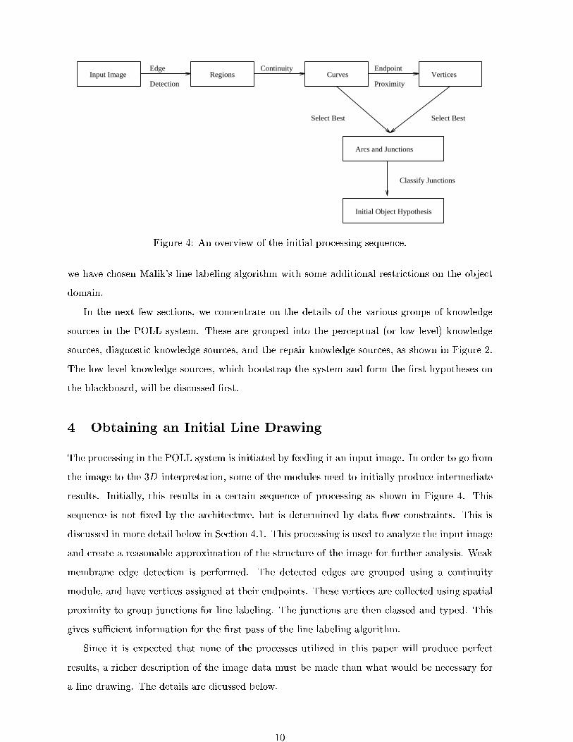
Figure 4: An overview of the initial processing sequence.
we have chosen Malik's line labeling algorithm with some additional restrictions on the object
domain.
In the next few sections, we concentrate on the details of the various groups of knowledge
sources in the POLL system. These are grouped into the perceptual (or low level) knowledge
sources, diagnostic knowledge sources, and the repair knowledge sources, as shown in Figure 2.
The low level knowledge sources, which bootstrap the system and form the �rst hypotheses on
the blackboard, will be discussed �rst.
4 Obtaining an Initial Line Drawing
The processing in the POLL system is initiated by feeding it an input image. In order to go from
the image to the 3D interpretation, some of the modules need to initially produce intermediate
results. Initially, this results in a certain sequence of processing as shown in Figure 4. This
sequence is not �xed by the architecture, but is determined by data ow constraints. This is
discussed in more detail below in Section 4.1. This processing is used to analyze the input image
and create a reasonable approximation of the structure of the image for further analysis. Weak
membrane edge detection is performed. The detected edges are grouped using a continuity
module, and have vertices assigned at their endpoints. These vertices are collected using spatial
proximity to group junctions for line labeling. The junctions are then classed and typed. This
gives suÆcient information for the �rst pass of the line labeling algorithm.
Since it is expected that none of the processes utilized in this paper will produce perfect
results, a richer description of the image data must be made than what would be necessary for
a line drawing. The details are dicussed below.
10
4.1 The Representation of Piecewise Continuous Objects in a Blackboard
The blackboard database contains a variety of data, including the initial intensity image, the
regions, curves, vertices, and object hypotheses that are output by the knowledge sources. To
discuss the organization of the blackboard system being used in this research, some vocabulary
is needed. The terms that are used here are those used in GBB (Generic Blackboard), the
blackboard shell used to implement POLL, and are given in [58]. The term \blackboard" used
by GBB will be replaced with \GBB blackboard" so as not to confuse the generic blackboard
ideas discussed before with the speci�c implementation of those ideas in GBB.
A GBB blackboard is a hierarchical tree structure composed of GBB blackboards and spaces.
Spaces are used to contain and index units. Units are the basic blackboard objects. When a
unit is created it is stored on a space. Such a unit is said to have been instantiated. Spaces are
stored, in turn, on a GBB blackboard. Indexing of units on spaces is optional in GBB, but in
image processing it can improve the eÆciency.
Units hold the hypotheses for entities that are found in the image. For the curvilinear line
labeling paradigm, for example, there are units for the arcs and the junctions. Each unit can
store three types of information. Slots hold the basic data, such as the name and label of a
junction. Indexes determine how the unit will be stored on the space. GBB permits a wide
range of indexing possibilities, including Frenet box ranges which are useful for units which are
not restricted to a single point. The �nal type of information is a link. Links relate a given unit
to other units. Di�erent types of units may be related using links.
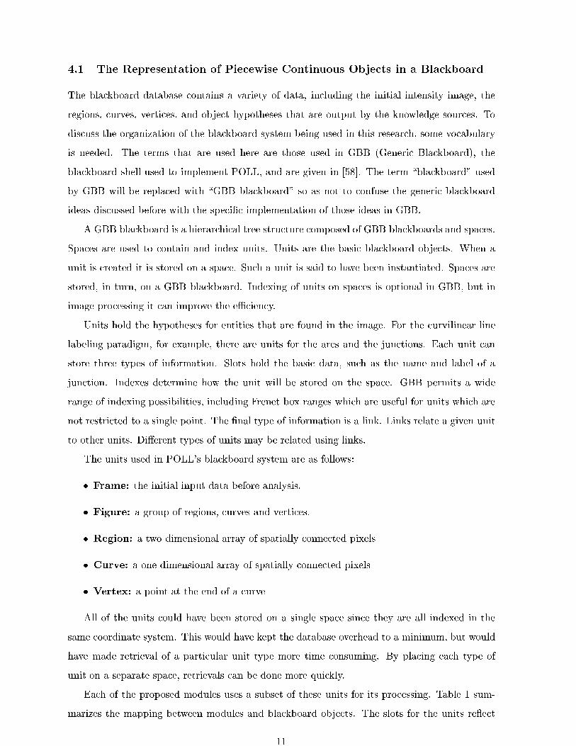
The units used in POLL's blackboard system are as follows:
� Frame: the initial input data before analysis.
� Figure: a group of regions, curves and vertices.
� Region: a two dimensional array of spatially connected pixels
� Curve: a one dimensional array of spatially connected pixels
� Vertex: a point at the end of a curve
All of the units could have been stored on a single space since they are all indexed in the
same coordinate system. This would have kept the database overhead to a minimum, but would
have made retrieval of a particular unit type more time consuming. By placing each type of
unit on a separate space, retrievals can be done more quickly.
Each of the proposed modules uses a subset of these units for its processing. Table 1 sum-
marizes the mapping between modules and blackboard objects. The slots for the units re ect
11
the needs of the modules using that unit. Some slots store information that is used by only
one module. As an example, the frame unit stores the �lename of the input data, and all units
have index variables stored. All units have a belief slot which gives a rough interpretation of
the importance of this unit at the given point in time. If a hypothesis has belief zero, it is not
used in further processing although it remains on the space. Although removing a hypothesis
with belief 0 would save storage space and speed retrievals, it would violate one of the design
goals by making recovery from mistakes impossible.
The links between units can be divided into four categories. All links are bidirectional, al-
though this is not dictated by GBB but rather by the needs of this application. Adjacency links
describe spatial adjacency relationships. An example of an adjacency link is the neighboring-
curves link in the curve unit. This link joins two curve units that are spatially adjacent. Ad-
jacency links can also join di�erent unit types. An example of this is the link between regions
and their boundary curves. The region side of the link is called bounded-by-curve, and the
curve side is called bounds-region. A second type of link also exists between regions and curves.
This link is used for curves that are in the interior of regions. Units of the same type are also
linked as supporting-hypotheses and competing-hypotheses. The �nal class of links used are
supplementary hypotheses. An example of a supplementary hypothesis is a missing edge that is
hypothesized from a line labeling failure.
As we pointed out before, the processing sequence in Figure 4 is not �xed by architecture
but is a consequence of the data ow constraints in the processing. Since the knowledge sources
are independent, they do not call each other directly. The initial processing is controlled by the
blackboard itself. As an example, the creation of a new region triggers the curvilinear grouping
module to create the edges. This is not done by the module that created the new region, but
is done as a consequence of placing a new region on the blackboard. Similarly, the curvilinear
grouping module does not directly call the vertex module. The vertex module is automatically
called by the blackboard when the curve unit is instantiated and placed on the blackboard. This
type of processing greatly enhances the consistency of the blackboard.
4.2 Creating the Initial Blackboard
Since the initial blackboard database is the foundation for all future processing, it is important
that it be an accurate representation of the important events in the image plane. It is not
necessary that it be perfect. In fact, if it were possible to reliably create a perfect initial
blackboard database, the integration that is the subject of this paper would be unnecessary.
During the initial analysis of the input image, competing hypotheses for image events are
12
instantiated. These competing hypotheses will make it possible to backtrack and correct poor
initial decisions at a later point in time when global constraints are applicable. With this
strategy, operations like thresholding that are normally fragile can be used with more con�dence.
The �rst line drawing hypothesis is created in three parts. Section 4.2.1 describes the sepa-
ration of the frame into coherent regions. In Section 4.2.2, the processing which starts with the
region units and creates a competing set of curve and vertex units is described. Once the curve
and vertex units have been established, the junctions need to have the number of incident arcs
in the initial �gure hypothesis identi�ed, and type (i.e. three tangent, curvature-L) determined.
4.2.1 Finding Regions
The purpose of the initial processing is to create a reasonable representation of the region, curve
and vertex units from the frame unit. All of the processing described in this section is of a local
nature. Local processing is advantageous at the early stages because it is potentially massively
parallel, although this virtue is not exploited in this implementation. The disadvantage of local
processing is that information in a small neighborhood is not always reliable in a more global
context. Since it is known that the information may not be globally reliable, alternate hypotheses
are kept. This makes it possible for later processing to backtrack and reverse decisions that were
good locally, but which fail in a more global setting.
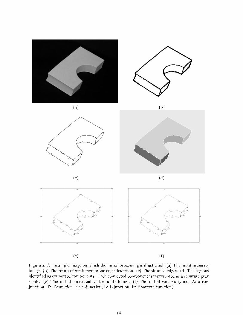
The processing in this section will be demonstrated using the image in Figure 5. This
image was captured in the Pattern Recognition and Image Processing (PRIP) laboratory at the
Michigan State University.
The �rst step in the processing of the real image is to �nd the edges using the region
based edge detection. As was discussed in Section 3.1, the weak membrane model with GNC
algorithm is used for edge detection. Although GNC claims to produce thin edges, it did not
always in practice. The reason for this failure was that many of the edges in the processed
images were ramp edges instead of step edges. This was caused by two factors. The �rst factor
is discretization error. Since the division between regions does not always coincide with the
division between pixels, some pixels will contain a mixture of two regions. This produces a
narrow ramp edge instead of a crisp step edge. The second reason for GNC to produce thick
edges is that some of the objects (bath tub toys) that were imaged do not have at sides. The
sides of the toys that appear to be planar are slightly curved. This curving produces ramp edges
instead of the step edges that GNC expects.
GNC responds to the ramp edges as repeated step edges and produces thick edges. The
edges found by GNC when run on the image in Figure 5(a) are shown in Figure 5(b). Although
13
(a) (b)
(c) (d)
.................................................................................................................................................................................................................................................
....................
.....................................................
..............
..........................................................................................
....................
...............
..........................................................................................................
...................
..............................................
................................................................
....................
.............
.............
.........
..........
........
.........
.........
........
..........
..........
.........
.........
.........
.........
...........
..........
....
....
...
................
..............
..............
............
.......
.............
.................
.............
.............
............
............
............
............
.....
...................................................................................................................................................................................................................................................................................................................................................................................................................................................................................................................................................................................................................................................................................................................................................................................................................................................................................................................
v51
v53
v4
v43
v54
v44
v13
v49
v45
v6
v36
v46
v38
v20
v47
v48
v50
v52
c33
c3c38
c4c47
c28
c15
c39
c12
c10
c42
c16c53
c44
c26
c23
c45c22
c20
c30
c32
c31
.................................................................................................................................................................................................................................................
....................
.....................................................
..............
..........................................................................................
....................
...............
..........................................................................................................
...................
..............................................
................................................................
....................
.............
.............
.........
..........
........
.........
.........
........
..........
..........
.........
.........
.........
.........
...........
..........
....
....
...
................
..............
..............
............
.......
.............
.................
.............
.............
............
............
............
............
.....
...................................................................................................................................................................................................................................................................................................................................................................................................................................................................................................................................................................................................................................................................................................................................................................................................................................................................................................................
L
L
L
A
Y
A
L
L
A
T
Y
A
P
L
A
L
L
L
c33
c3c38
c4c47
c28
c15
c39
c12
c10
c42
c16c53
c44
c26
c23
c45c22
c20
c30
c32
c31
(e) (f)
Figure 5: An example image on which the initial processing is illustrated. (a) The input intensityimage. (b) The result of weak membrane edge detection. (c) The thinned edges. (d) The regionsidenti�ed as connected components. Each connected component is represented as a separate grayshade. (e) The initial curve and vertex units found. (f) The initial vertices typed (A: arrowjunction, T: T-junction, Y: Y-junction, L: L-junction, P: Phantom junction).
14
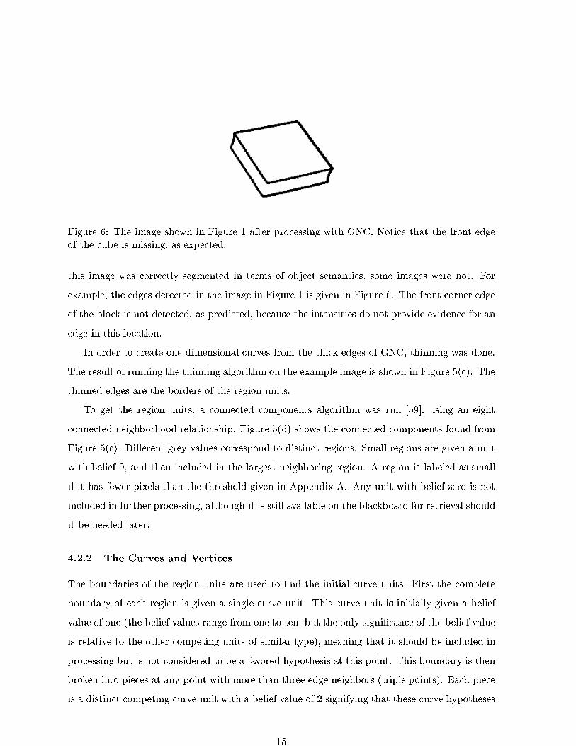
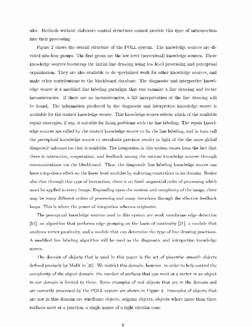
Figure 6: The image shown in Figure 1 after processing with GNC. Notice that the front edgeof the cube is missing, as expected.
this image was correctly segmented in terms of object semantics, some images were not. For
example, the edges detected in the image in Figure 1 is given in Figure 6. The front corner edge
of the block is not detected, as predicted, because the intensities do not provide evidence for an
edge in this location.
In order to create one dimensional curves from the thick edges of GNC, thinning was done.
The result of running the thinning algorithm on the example image is shown in Figure 5(c). The
thinned edges are the borders of the region units.
To get the region units, a connected components algorithm was run [59], using an eight
connected neighborhood relationship. Figure 5(d) shows the connected components found from
Figure 5(c). Di�erent grey values correspond to distinct regions. Small regions are given a unit
with belief 0, and then included in the largest neighboring region. A region is labeled as small
if it has fewer pixels than the threshold given in Appendix A. Any unit with belief zero is not
included in further processing, although it is still available on the blackboard for retrieval should
it be needed later.
4.2.2 The Curves and Vertices
The boundaries of the region units are used to �nd the initial curve units. First the complete
boundary of each region is given a single curve unit. This curve unit is initially given a belief
value of one (the belief values range from one to ten, but the only signi�cance of the belief value
is relative to the other competing units of similar type), meaning that it should be included in
processing but is not considered to be a favored hypothesis at this point. This boundary is then
broken into pieces at any point with more than three edge neighbors (triple points). Each piece
is a distinct competing curve unit with a belief value of 2 signifying that these curve hypotheses
15
are more perceptually signi�cant than the initial ones and should take precedence in processing.
If no competing hypotheses are found, the initial curve hypothesis has its belief raised to 2,
meaning that it has gained perceptual signi�cance. The curvilinearity algorithm described in
[21] is then run on the triple point curve units, or the original boundary curve unit if it was
unbroken by vertices. If corners are found by the continuity algorithm, competing curve units
are created for each segment, with a belief value of three. If no corners were found, the previous
curve hypothesis has its belief value raised to three. This leaves a unique hypothesis that is
thought to be best at each of the points on the boundary of the region. Since the continuity
algorithm is consistently �nding better hypotheses than what triple points alone could provide,
these hypotheses are given the highest con�dence of the three curves initially. At the end of
each of these curve units, a vertex unit is instantiated.
There are edge points that are found by GNC that do not fall on the boundary of a region.
Some of these points are caused by hairs left on the edges by GNC that have been thinned.
Some of the other edges on the interior of a region are partially detected edges. To collect
these edges into reasonable structures, the edges that are not on the boundary for each region
are grouped using the curvilinear grouping algorithm. By grouping only within single detected
regions, undesirable groupings between distinct regions are eliminated. These groupings are
given a belief value of three if they are more than a few pixels long (the threshold value is given
in Appendix A), and a belief value of zero otherwise.
At this point, a set of competing curve units has been created. Each curve unit will have
either no endpoints (as with the boundary of an isolated sphere), or two endpoints. Some of
the curve units are only a few pixels long, particularly those near the corners of the regions.
Competing vertex units have not yet been created. Since the continuity algorithm typically
leaves several bends near a vertex, particularly when working with real data, these small curves
and vertices need to be combined. The method for doing this initially is simple. When a vertex is
created, it tries to join with any other vertex in a local neighborhood to create a stronger vertex.
The size of this local neighborhood is determined by a threshold, shown in Appendix A. If a
vertex is combined, the old vertex is given a belief zero. An artifact of this vertex combination
is that there are short curves with both endpoints at the same combined vertex. These curve
units are given a belief zero. This cleans away many short, perceptually unimportant curves.
This processing results in an initial set of vertices and curves that form the �rst �gure
hypothesis. The result for the example image in Figure 5(a) is shown in Figure 5(e). The
labeling scheme is as follows. Curves are labeled with the letter \c" and an identi�cation
number. Vertices are labeled with the letter \v" and an identi�cation number. The label for a
16
curve is placed to the lower left of the middle of a curve. The label for a vertex is placed at the
vertex. Around the edge of the image is a frame that completes any junctions that reach the
edge of the image. This frame will be shown in all future images, and is labeled a priori as a
jump edge.
At this point the blackboard contains regions, a group of competing curve units, and a group
of competing vertex units. Within the groups of both curve units and vertex units the competing
units have been labeled with belief values to determine which appears to be best at this point
in time. The blackboard also contains the beginning of the �rst �gure unit: the collection of
all non-competing curve units of highest belief value and the collection of all non-competing
vertex units of the highest belief value. For the �gure unit to be complete the vertices must be
classi�ed and typed. These operations are discussed next.
4.2.3 Identifying Junctions
First vertex units are classi�ed by the number of incident arcs. This classi�cation yields four
categories, junctions with one incoming arc, junctions with two incoming arcs, junctions with
three incoming arcs, and junctions with four or more incoming arcs. The domain assumptions
made in this work exclude vertices with more than three arcs, so junctions in the fourth category
are outside the scope of this paper and can be agged as erroneous immediately. The domain
of piecewise smooth surfaces discussed in [30] does not have this restriction.
A much more challenging problem than classifying the junctions is typing them. A summary
of the attributes that determine junction type is given in Table 2. The table does not distinguish
between Arrow and Y junctions. This distinction is made by examining the angle between the
incoming arcs. If one of the angles is greater than 180Æ, the junction is an Arrow. If all three
angles measure less than 180Æ the junction is a Y.
In order to assign a type to the junctions, each of the curve units must have a tangent
and curvature value at both endpoints. Finding curvature is a diÆcult problem. Therefore
the curvature values that are calculated should be treated with suspicion. Estimating tangent
direction is somewhat easier. Since later processing can help to correct mistakes, it is not essential
that the curvatures and tangents be perfect. Curvature and tangent direction estimations are
regularized using the continuity module to preprocess all curves. This module smooths the
curves, removes outliers, and separates the curve at discontinuities. Without this preprocessing,
the estimations would be more unreliable.
The simplest way to �nd curvature is to �t a circle to a set of points, and �nd the radius
and the center. The multiplicative inverse of the radius is the curvature. A normal to the �t
17
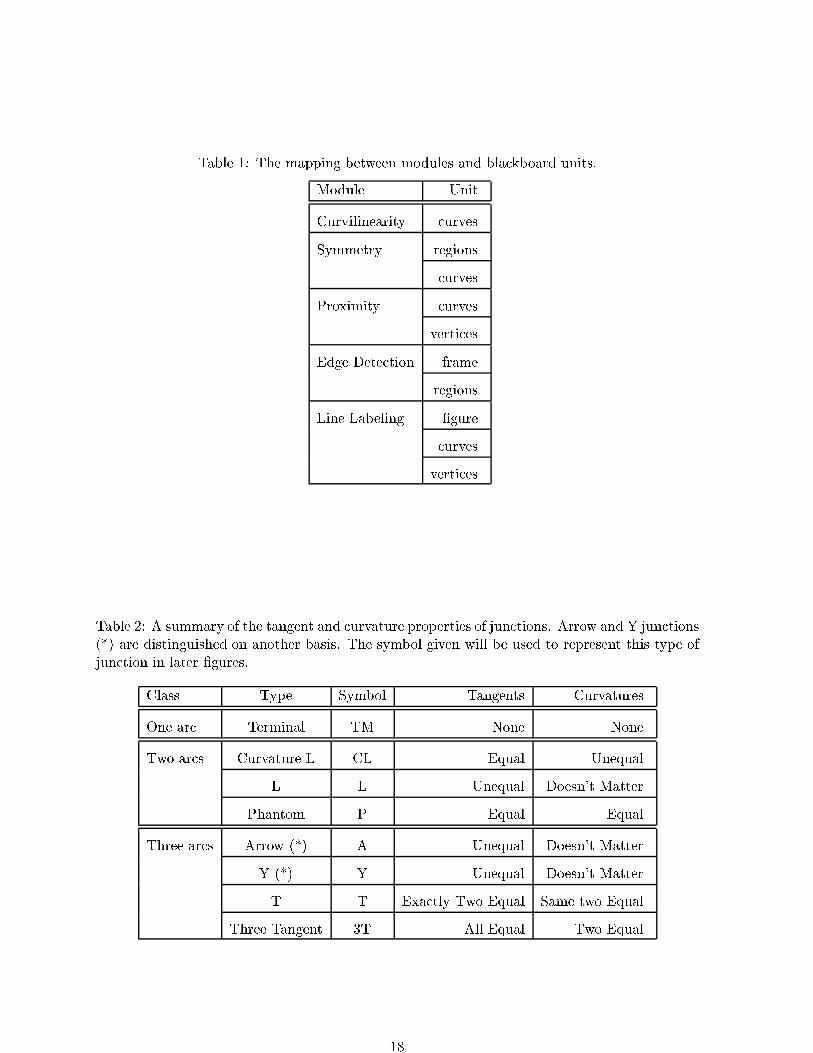
Table 1: The mapping between modules and blackboard units.
Module Unit
Curvilinearity curves
Symmetry regions
curves
Proximity curves
vertices
Edge Detection frame
regions
Line Labeling �gure
curves
vertices
Table 2: A summary of the tangent and curvature properties of junctions. Arrow and Y junctions(*) are distinguished on another basis. The symbol given will be used to represent this type ofjunction in later �gures.
Class Type Symbol Tangents Curvatures
One arc Terminal TM None None
Two arcs Curvature L CL Equal Unequal
L L Unequal Doesn't Matter
Phantom P Equal Equal
Three arcs Arrow (*) A Unequal Doesn't Matter
Y (*) Y Unequal Doesn't Matter
T T Exactly Two Equal Same two Equal
Three Tangent 3T All Equal Two Equal
18
circle at the endpoint can be found from the vector starting at the center of the circle and
ending at the endpoint of the arc. The tangent direction is perpendicular to the normal. The
�tting is done using a nonlinear least squares method found in [60]. Circular arcs were �t in
a neighborhood of the endpoint, with the size of the neighborhood determined by a parameter
given in Appendix A.
Although a straight line can be thought of as a circle of in�nite radius, this is numerically
troublesome. To avoid this problem, straight lines are �t in a neighborhood of the endpoint. The
size of this neighborhood is determined by a parameter given in Appendix A. The curvature for
a straight line is zero, and the tangent direction is calculated from the slope. The squared error,
calculated in units of pixels squared, between the circular �t and the linear �t is then compared
and the model with the better �t is accepted. The curvature values calculated in this fashion
are rough estimates. Therefore comparisons like those suggested in Table 2 must be revised.
Even with synthetic data, it is unlikely that two curvatures or tangents would be exactly equal.
To compare tangent directions, a threshold was used on the di�erence. This threshold is given
in Appendix A. This threshold was set arbitrarily, but is not critical to the performance of the
system since later processing can change this threshold to correct mistakes.
The curvature values were found to be very unreliable, particularly in the real images that
were used. There are several reasons for this. The objects used in the images in this paper
have circular arcs, which project to ellipses. Fitting a circle to an ellipse, particularly at the
ends of the major axis where the curvature is changing rapidly is diÆcult. Another problem is
that the continuity algorithm may not break the upper and lower halves of an ellipse exactly at
the corner. This means that the curvature will be calculated starting at di�erent places on the
ellipse, which will certainly lead to di�erent curvatures. To get around this problem, curvatures
were placed into only three classes, which are described in Appendix A. Curvatures will be
considered to be equivalent if they fall into the same class. It would have been possible to �t
an ellipse to the curve data instead of a circle, but this is computationally more expensive and
unnecessary.
With the curvature and tangent information, and suitable de�nitions of equivalence among
tangents and curvatures, the classi�ed vertices in the initial �gure unit can be typed. This
information completes the initial �gure unit, that is the �rst hypothesis for the arcs and junctions
in the imaged scene.
Although errors in the initial processing can be repaired later, it is important that the �rst
�gure unit be an accurate representation of most of the important events in the image plane.
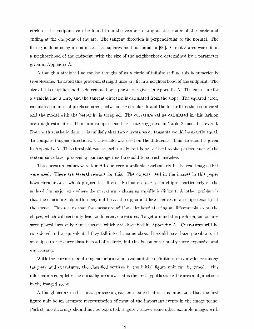
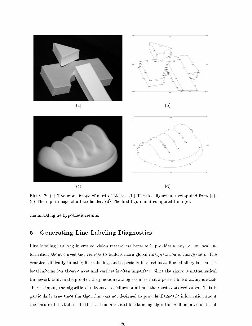
Perfect line drawings should not be expected. Figure 7 shows some other example images with
19
.................................................................................................................................................................................................................................................
........
.......................
........
........
........
........
........
..........................
..
........
........
........
........
........
.......
........
........
......
....................................................................
.................................................................
........
...........
........
........
........
........
........
...
.................
..................................
............................
.......................................
.....................................................................................
...
............................................................................................................................
..................................................
...
........
....
....
.....
..........
.........................................
.......
....
........
...........................
.................
...............
.................
..............
.................................................................................
..........
............................................................
.......................
.............................
............................
....................................................................................
......................................................
........................................
....................
..................................................................
........
........
.......
........
........
.......
........
........
........
.....
...................................................................................
...................
...................................................................................................................................................................................................................................................................................................................................................................................................................................................................................................................................................................................................................................................................................................................................................................................................................................................................................................................
v100
v102
v36v95
v94
v96v93
v37
v104
v19
v105
v92
v91
v40
v98
v90
v97
v106
v107v108
v75
v89
v109
v111
v9
v17
v88
v52
v103
v3
v110
v84
v14
v86v85
v87
v99
v101
c50
c36
c34
c29
c32
c37
c64
c99
c27
c66
c25
c23
c42
c21
c38c41
c70
c68
c73
c19c72
c75
c95
c76c17
c16
c15
c53
c60
c56
c55
c78
c46
c2
c52
c13
c5
c7
c80
c12
c10
c47
c49
c48
(a) (b)
............................................................................................................................................................................................................................................
...........
............................................
..........
.................
.....................................................................................
.........
........
........
.......
........
........
.........
..............
........
.........
.........
...
....
.........
........
........
........
........
..........
..............
....................................
.........................................................................................................................................
.....................
..................
.............
..........
........
.......
...............................
....
....
............
........
.........
...........
.......
.........
.........
...........................................................................................................................................................................
............
........
............
........
........
........
........
............
....
......................................................
.....................................
.......................................................
..........................
........................................................................................................................................................................................................................................................................................................................................................................................................................................................................................................................................................................ ............................................................................................................................................................................................................................................................................................................................
L
L
TM
P
PCL
TM
CL
TM
T
TM
T
TM
TM
T
P
TTM
T
P
L
L
L
c26
c20c21
c92
c90
c22
c3
c88
c98c89
c4
c16
c91
c6
c94
c7
c9
c13
c11
c23
c25
c24
(c) (d)
Figure 7: (a) The input image of a set of blocks. (b) The �rst �gure unit computed from (a).(c) The input image of a taco holder. (d) The �rst �gure unit computed from (c).
the initial �gure hypothesis results.
5 Generating Line Labeling Diagnostics
Line labeling has long interested vision researchers because it provides a way to use local in-
formation about curves and vertices to build a more global interpretation of image data. The
practical diÆculty in using line labeling, and especially in curvilinear line labeling, is that the
local information about curves and vertices is often imperfect. Since the rigorous mathematical
framework built in the proof of the junction catalog assumes that a perfect line drawing is avail-
able as input, the algorithm is doomed to failure in all but the most contrived cases. This is
particularly true since the algorithm was not designed to provide diagnostic information about
the nature of the failure. In this section, a revised line labeling algorithm will be presented that
20
can provide some diagnostic information about line labeling failures.
5.1 Detection of Line Drawing Problems
The algorithms that have been used in Section 4 to extract line drawings from images cannot
produce perfect output. Therefore it is important to be able to analyze a line drawing and
evaluate its strengths and weaknesses. This section will show a modi�cation to the standard
line labeling scheme proposed by Malik [30] which provides better diagnostic information about
the weaknesses of the current line drawings. This diagnostic information will be entered into
the blackboard database and later be used by other modules to �x problems in the line drawing.
The line labels used for the domain of piecewise smooth objects are the following:
!! A limb edge is a depth discontinuity that is formed when the line of sight is tangent to
the surface and the surface occludes itself with respect to the viewpoint. The direction of
the arrow is selected such that the surface closest to the viewer is on the right hand side
of the arrow as it is followed from tail to head.
! A jump edge which is a depth discontinuity which is not a limb edge.
+ A convex edge where the visible angle between the surfaces is greater than 180Æ.
� A concave edge where the visible angle between the surfaces is smaller than 180Æ.
In the piecewise smooth object domain, the junction catalog is guaranteed to give one or
more correct labelings for each object in the object domain. An object that is not within this
domain may still be legally, and perhaps even correctly, labeled. To restate this in a way that
is more relevant to this discussion: there is no guarantee that if a mistake is made in the initial
line drawing that line labeling will fail to interpret the image. Therefore, line labeling cannot
be the only arbiter of correctness in line drawings. However, when possible, it can contribute
towards this goal. This section will demonstrate how line labeling can be instrumental in �xing
incorrect line drawings.
One of the diÆculties with using line labeling as a diagnostic tool is that there are often
multiple interpretations of a single object. To reduce the combinatorics of the line labeling, the
POLL system uses a heuristic called the oating object heuristic to initiate labeling of the line
drawings. We assume that the image has been segmented into regions. Further, we assume that
these regions have been correctly labeled as either background or foreground. The objects of
interest should be in the foreground. The labeling of the background region is a method for
performing �gure-ground separation, which is one of the Gestalt principles. This �gure-ground
21
separation is done by hand in the POLL system, although it would be preferable to have the
system select the background automatically. Using this terminology, the heuristic is de�ned as
follows:
De�nition 1 Floating Object Heuristic: All outside arcs (that is, those that are adjacent to
the background region) in a line labeling should be labeled as either limb or jump edges with
the direction being such that the foreground region will be interpreted as being in front of the
background region. The labels on inside arcs are not restricted.
There are times when the oating object heuristic won't work, such as when part of an
object is being viewed through a hole. A similar heuristic was used before by Winston [61]. Line
labeling with the oating object heuristic is much less combinatorially explosive than ordinary
line labeling. There are two contributing factors. The �rst factor is that there are fewer interpre-
tations of outside junctions. A casual inspection of Malik's original junction catalog, shows that
most of the legal interpretations for inside junctions will no longer be legal interpretations for
outside junctions thus reducing the number of possibilities. A second factor that improves the
combinatorics of line labeling is that phantom junctions are not necessary with this heuristic,
since a necessary phantom junction can be identi�ed by the line labeling process.
If an image can be segmented into foreground and background regions, outside junctions
that have been labeled by the oating object heuristic will have at most two interpretations,
except for T junctions which may have as many as four interpretations. This can be veri�ed by
a case analysis on the junction catalogue and a counting argument.
Table 3 shows a vast improvement in combinatorics for outside junctions with the oating
object heuristic. Five di�erent outside junctions have a unique labeling with the oating object
heuristic. These unique labelings of arcs on a local basis will improve the combinatorics of
labeling inside arcs as well. This combinatoric improvement can also be exploited to improve
the line labeling paradigm. Outside arcs and outside junctions are providing the strongest
constraints. When this information is used �rst in the line labeling algorithm, the legal labelings
on the inside arcs are also restricted. Algorithm 1 is the modi�ed line labeling algorithm which
takes advantage of this combinatoric reduction and which provides diagnostic feedback.
The principal advantage of Algorithm 1 over the three step algorithm proposed by Malik
in [30] is that diagnostic information is provided for the blackboard in the form of the failed
vertex. Since the number of legal line labelings is often reduced to a single set by the improved
combinatorics, this diagnostic information can pinpoint the area of the line drawing that is
incorrect. This makes it possible to make corrections. Figure 9 shows the curves and vertices
identi�ed for the image in Figure 1. When the modi�ed line labeling algorithm is run on this
22
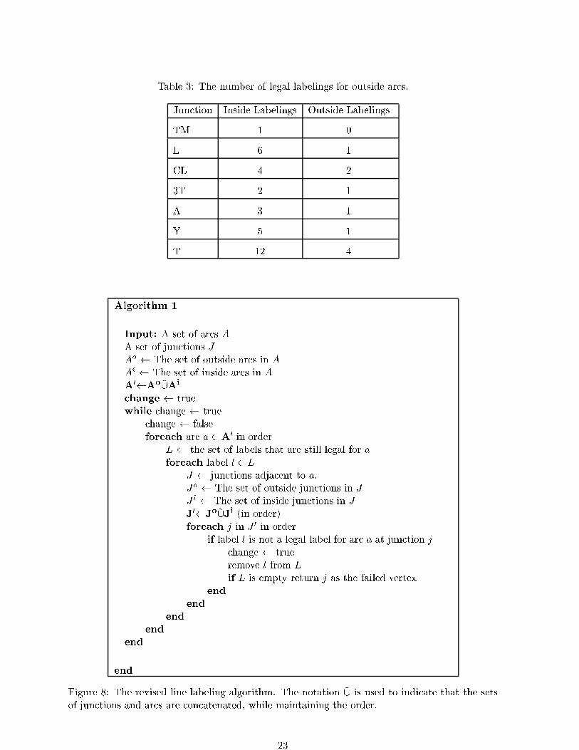
Table 3: The number of legal labelings for outside arcs.
Junction Inside Labelings Outside Labelings
TM 1 0
L 6 1
CL 4 2
3T 2 1
A 3 1
Y 5 1
T 12 4
Algorithm 1
Input: A set of arcs AA set of junctions JAo The set of outside arcs in A
Ai The set of inside arcs in A
A0 Ao~[Ai
change truewhile change true
change falseforeach arc a 2 A0 in order
L the set of labels that are still legal for aforeach label l 2 L
J junctions adjacent to a.Jo The set of outside junctions in J
J i The set of inside junctions in J
J0 Jo~[Ji (in order)
foreach j in J 0 in orderif label l is not a legal label for arc a at junction j
change trueremove l from L
if L is empty return j as the failed vertexend
end
end
end
end
end
Figure 8: The revised line labeling algorithm. The notation ~[ is used to indicate that the setsof junctions and arcs are concatenated, while maintaining the order.
23
.................................................................................................................................................................................................................................................
....
............
........
........
........
........
........
........
........
........
........
........................................
..................................
...........................
.....................................
...................................
.............................
..........................................................................
.................................................................................................
.............................................................................
.................
...................................................................................................................................................................................................................................................................................................................................................................................................................................................................................................................................................................................................................................................................................................................................................................................................................................................................................................................
v33
v35
v28
v30
v31
v25
v6
v27
v29
v32
v34
c19
c8
c12
c24
c6
c23
c14
c5
c3
c16
c18
c17
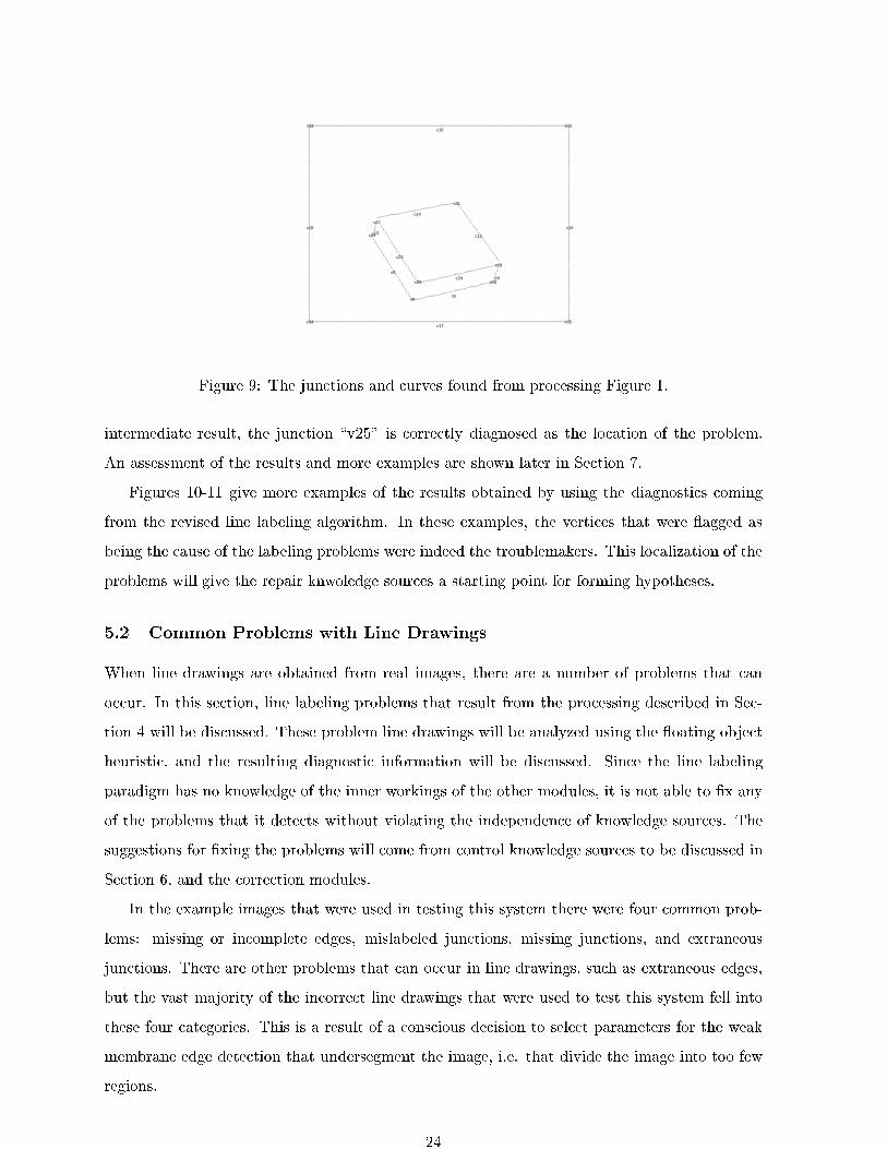
Figure 9: The junctions and curves found from processing Figure 1.
intermediate result, the junction \v25" is correctly diagnosed as the location of the problem.
An assessment of the results and more examples are shown later in Section 7.
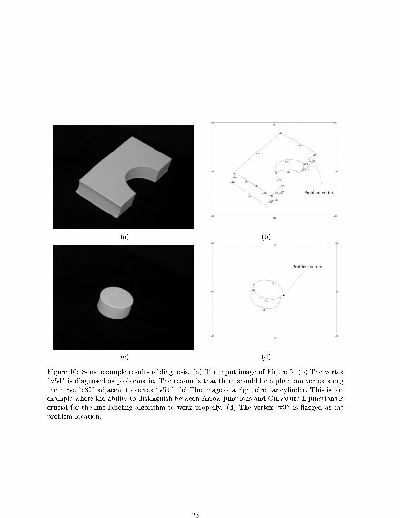
Figures 10-11 give more examples of the results obtained by using the diagnostics coming
from the revised line labeling algorithm. In these examples, the vertices that were agged as
being the cause of the labeling problems were indeed the troublemakers. This localization of the
problems will give the repair knwoledge sources a starting point for forming hypotheses.
5.2 Common Problems with Line Drawings
When line drawings are obtained from real images, there are a number of problems that can
occur. In this section, line labeling problems that result from the processing described in Sec-
tion 4 will be discussed. These problem line drawings will be analyzed using the oating object
heuristic, and the resulting diagnostic information will be discussed. Since the line labeling
paradigm has no knowledge of the inner workings of the other modules, it is not able to �x any
of the problems that it detects without violating the independence of knowledge sources. The
suggestions for �xing the problems will come from control knowledge sources to be discussed in
Section 6, and the correction modules.
In the example images that were used in testing this system there were four common prob-
lems: missing or incomplete edges, mislabeled junctions, missing junctions, and extraneous
junctions. There are other problems that can occur in line drawings, such as extraneous edges,
but the vast majority of the incorrect line drawings that were used to test this system fell into
these four categories. This is a result of a conscious decision to select parameters for the weak
membrane edge detection that undersegment the image, i.e. that divide the image into too few
regions.
24
.................................................................................................................................................................................................................................................
....................
.....................................................
..............
..........................................................................................
....................
...............
..........................................................................................................
...................
..............................................
................................................................
....................
.............
.............
.........
..........
........
.........
.........
........
..........
..........
.........
.........
.........
.........
...........
..........
....
....
...
................
..............
..............
............
.......
.............
.................
.............
.............
............
............
............
............
.....
...................................................................................................................................................................................................................................................................................................................................................................................................................................................................................................................................................................................................................................................................................................................................................................................................................................................................................................................
v51
v53
v4
v43
v54
v44
v13
v49
v45
v6
v36
v46
v38
v20
v47
v48
v50
v52
c33
c3c38
c4c47
c28
c15
c39
c12
c10
c42
c16c53
c44
c26
c23
c45c22
c20
c30
c32
c31
Problem vertex
(a) (b).................................................................................................................................................................................................................................................
................
........................
.......
...........
......................................................
................................................................................................
.......................
.........................................................................
...................................................................................................................................................................................................................................................................................................................................................................................................................................................................................................................................................................................................................................................................................................................................................................................................................................................................................................................
v17
v19
v3
v4
v15
v16
v18
c9c5
c4
c2
c11
c6
c8
c7
Problem vertex
(c) (d)
Figure 10: Some example results of diagnosis. (a) The input image of Figure 5. (b) The vertex\v54" is diagnosed as problematic. The reason is that there should be a phantom vertex alongthe curve \c39" adjacent to vertex \v54." (c) The image of a right circular cylinder. This is oneexample where the ability to distinguish between Arrow junctions and Curvature L junctions iscrucial for the line labeling algorithm to work properly. (d) The vertex \v3" is agged as theproblem location.
25
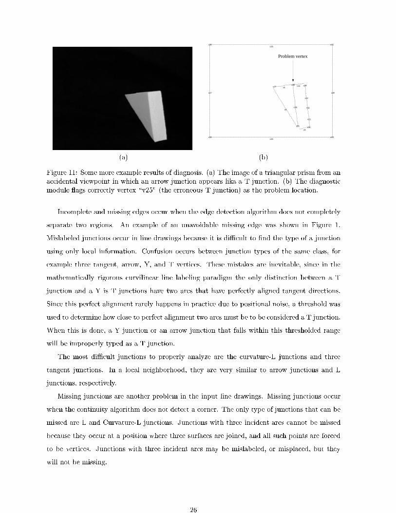
.................................................................................................................................................................................................................................................
...
.................
....
...........................
............................
............................................................
..........................
..............................................................................................................
......................................................................................................
..................................................
...................................................................................................................................................................................................................................................................................................................................................................................................................................................................................................................................................................................................................................................................................................................................................................................................................................................................................................................
v31
v33
v28
v11
v29
v26
v25v27
v30
v32
c18
c11
c14
c12
c9
c25c6
c3
c15
c17
c16
Problem vertex
(a) (b)
Figure 11: Some more example results of diagnosis. (a) The image of a triangular prism from anaccidental viewpoint in which an arrow junction appears lika a T junction. (b) The diagnosticmodule ags correctly vertex \v25" (the erroneous T junction) as the problem location.
Incomplete and missing edges occur when the edge detection algorithm does not completely
separate two regions. An example of an unavoidable missing edge was shown in Figure 1.
Mislabeled junctions occur in line drawings because it is diÆcult to �nd the type of a junction
using only local information. Confusion occurs between junction types of the same class, for
example three tangent, arrow, Y, and T vertices. These mistakes are inevitable, since in the
mathematically rigorous curvilinear line labeling paradigm the only distinction between a T
junction and a Y is T junctions have two arcs that have perfectly aligned tangent directions.
Since this perfect alignment rarely happens in practice due to positional noise, a threshold was
used to determine how close to perfect alignment two arcs must be to be considered a T junction.
When this is done, a Y junction or an arrow junction that falls within this thresholded range
will be improperly typed as a T junction.
The most diÆcult junctions to properly analyze are the curvature-L junctions and three
tangent junctions. In a local neighborhood, they are very similar to arrow junctions and L
junctions, respectively.
Missing junctions are another problem in the input line drawings. Missing junctions occur
when the continuity algorithm does not detect a corner. The only type of junctions that can be
missed are L and Curvature-L junctions. Junctions with three incident arcs cannot be missed
because they occur at a position where three surfaces are joined, and all such points are forced
to be vertices. Junctions with three incident arcs may be mislabeled, or misplaced, but they
will not be missing.
26
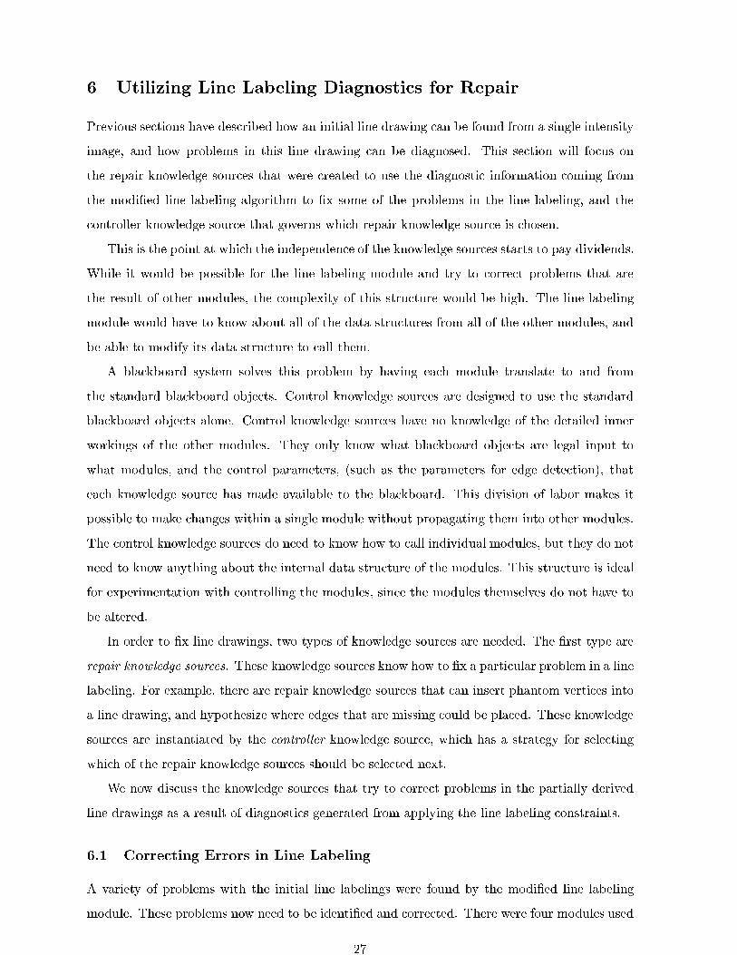
6 Utilizing Line Labeling Diagnostics for Repair
Previous sections have described how an initial line drawing can be found from a single intensity
image, and how problems in this line drawing can be diagnosed. This section will focus on
the repair knowledge sources that were created to use the diagnostic information coming from
the modi�ed line labeling algorithm to �x some of the problems in the line labeling, and the
controller knowledge source that governs which repair knowledge source is chosen.
This is the point at which the independence of the knowledge sources starts to pay dividends.
While it would be possible for the line labeling module and try to correct problems that are
the result of other modules, the complexity of this structure would be high. The line labeling
module would have to know about all of the data structures from all of the other modules, and
be able to modify its data structure to call them.
A blackboard system solves this problem by having each module translate to and from
the standard blackboard objects. Control knowledge sources are designed to use the standard
blackboard objects alone. Control knowledge sources have no knowledge of the detailed inner
workings of the other modules. They only know what blackboard objects are legal input to
what modules, and the control parameters, (such as the parameters for edge detection), that
each knowledge source has made available to the blackboard. This division of labor makes it
possible to make changes within a single module without propagating them into other modules.
The control knowledge sources do need to know how to call individual modules, but they do not
need to know anything about the internal data structure of the modules. This structure is ideal
for experimentation with controlling the modules, since the modules themselves do not have to
be altered.
In order to �x line drawings, two types of knowledge sources are needed. The �rst type are
repair knowledge sources. These knowledge sources know how to �x a particular problem in a line
labeling. For example, there are repair knowledge sources that can insert phantom vertices into
a line drawing, and hypothesize where edges that are missing could be placed. These knowledge
sources are instantiated by the controller knowledge source, which has a strategy for selecting
which of the repair knowledge sources should be selected next.
We now discuss the knowledge sources that try to correct problems in the partially derived
line drawings as a result of diagnostics generated from applying the line labeling constraints.
6.1 Correcting Errors in Line Labeling
A variety of problems with the initial line labelings were found by the modi�ed line labeling
module. These problems now need to be identi�ed and corrected. There were four modules used
27
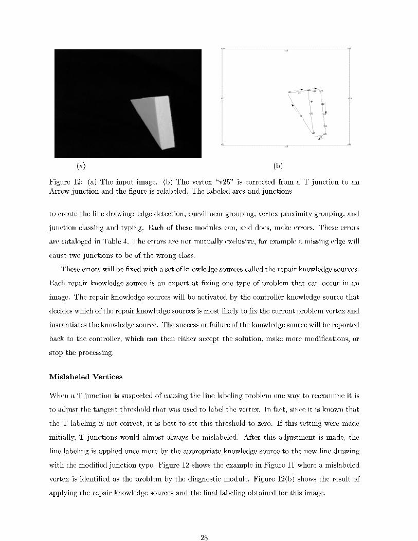
.................................................................................................................................................................................................................................................
...
.................
....
...........................
............................
............................................................
..........................
..............................................................................................................
......................................................................................................
..................................................
...................................................................................................................................................................................................................................................................................................................................................................................................................................................................................................................................................................................................................................................................................................................................................................................................................................................................................................................
v31
v33
v28
v11
v29
v26
v25v27
v30
v32
c18
c11
c14
c12
c9
c25c6
c3
c15
c17
c16
+
(a) (b)
Figure 12: (a) The input image. (b) The vertex \v25" is corrected from a T junction to anArrow junction and the �gure is relabeled. The labeled arcs and junctions
to create the line drawing: edge detection, curvilinear grouping, vertex proximity grouping, and
junction classing and typing. Each of these modules can, and does, make errors. These errors
are cataloged in Table 4. The errors are not mutually exclusive, for example a missing edge will
cause two junctions to be of the wrong class.
These errors will be �xed with a set of knowledge sources called the repair knowledge sources.
Each repair knowledge source is an expert at �xing one type of problem that can occur in an
image. The repair knowledge sources will be activated by the controller knowledge source that
decides which of the repair knowledge sources is most likely to �x the current problem vertex and
instantiates the knowledge source. The success or failure of the knowledge source will be reported
back to the controller, which can then either accept the solution, make more modi�cations, or
stop the processing.
Mislabeled Vertices
When a T junction is suspected of causing the line labeling problem one way to reexamine it is
to adjust the tangent threshold that was used to label the vertex. In fact, since it is known that
the T labeling is not correct, it is best to set this threshold to zero. If this setting were made
initially, T junctions would almost always be mislabeled. After this adjustment is made, the
line labeling is applied once more by the appropriate knowledge source to the new line drawing
with the modi�ed junction type. Figure 12 shows the example in Figure 11 where a mislabeled
vertex is identi�ed as the problem by the diagnostic module. Figure 12(b) shows the result of
applying the repair knowledge sources and the �nal labeling obtained for this image.
28
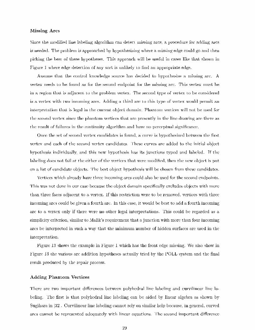
Missing Arcs
Since the modi�ed line labeling algorithm can detect missing arcs, a procedure for adding arcs
is needed. The problem is approached by hypothesizing where a missing edge could go and then
picking the best of these hypotheses. This approach will be useful in cases like that shown in
Figure 1 where edge detection of any sort is unlikely to �nd an appropriate edge.
Assume that the control knowledge source has decided to hypothesize a missing arc. A
vertex needs to be found as for the second endpoint for the missing arc. This vertex must be
in a region that is adjacent to the problem vertex. The second type of vertex to be considered
is a vertex with two incoming arcs. Adding a third arc to this type of vertex would permit an
interpretation that is legal in the current object domain. Phantom vertices will not be used for
the second vertex since the phantom vertices that are presently in the line drawing are there as
the result of failures in the continuity algorithm and have no perceptual signi�cance.
Once the set of second vertex candidates is found, a curve is hypothesized between the �rst
vertex and each of the second vertex candidates. These curves are added to the initial object
hypothesis individually, and this new hypothesis has its junctions typed and labeled. If the
labeling does not fail at the either of the vertices that were modi�ed, then the new object is put
on a list of candidate objects. The best object hypothesis will be chosen from these candidates.
Vertices which already have three incoming arcs could also be used for the second endpoints.
This was not done in our case because the object domain speci�cally excludes objects with more
than three faces adjacent to a vertex. If this restriction were to be removed, vertices with three
incoming arcs could be given a fourth arc. In this case, it would be best to add a fourth incoming
arc to a vertex only if there were no other legal interpretations. This could be regarded as a
simplicity criterion, similar to Malik's requirement that a junction with more than four incoming
arcs be interpreted in such a way that the minimum number of hidden surfaces are used in the
interpretation.
Figure 13 shows the example in Figure 1 which has the front edge missing. We also show in
Figure 13 the various arc addition hypotheses actually tried by the POLL system and the �nal
result produced by the repair process.
Adding Phantom Vertices
There are two important di�erences between polyhedral line labeling and curvilinear line la-
beling. The �rst is that polyhedral line labeling can be aided by linear algebra as shown by
Sugihara in [32]. Curvilinear line labeling cannot rely on similar help because, in general, curved
arcs cannot be represented adequately with linear equations. The second important di�erence
29
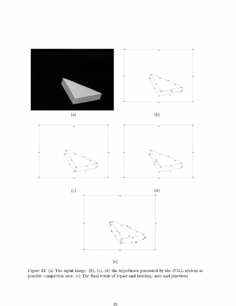
.................................................................................................................................................................................................................................................
....................
..............
..................
..................
............
............................................
..........................................
...........
...............................................
..........................................
..............
.......................
...................
...................
.................................................................................................
................................................................................
..................
...................................................................................................................................................................................................................................................................................................................................................................................................................................................................................................................................................................................................................................................................................................................................................................................................................................................................................................................
...............................................................................................
v29
v31
v27
v25
v12
v22
v6
v24
v26
v28
v30
c18
c8
c12
c22
c6
c13
c21
c5
c3
c15
c17
c16
c27
(a) (b)
.................................................................................................................................................................................................................................................
....................
..............
..................
..................
............
............................................
..........................................
...........
...............................................
..........................................
..............
.......................
...................
...................
.................................................................................................
................................................................................
..................
...................................................................................................................................................................................................................................................................................................................................................................................................................................................................................................................................................................................................................................................................................................................................................................................................................................................................................................................
.......................
v29
v31
v27
v25
v12
v22
v6
v24
v26
v28
v30
c18
c8
c12
c22
c6
c13
c21
c5
c3
c15
c17
c16
c28
.................................................................................................................................................................................................................................................
....................
..............
..................
..................
............
............................................
..........................................
...........
...............................................
..........................................
..............
.......................
...................
...................
.................................................................................................
................................................................................
..................
...................................................................................................................................................................................................................................................................................................................................................................................................................................................................................................................................................................................................................................................................................................................................................................................................................................................................................................................
............................................................
v29
v31
v27
v25
v12
v22
v6
v24
v26
v28
v30
c18
c8
c12
c22
c6
c13
c21
c5
c3
c15
c17
c16
c29
(c) (d).................................................................................................................................................................................................................................................
....................
..............
..................
..................
............
............................................
..........................................
...........
...............................................
..........................................
..............
.......................
...................
...................
.................................................................................................
................................................................................
..................
...................................................................................................................................................................................................................................................................................................................................................................................................................................................................................................................................................................................................................................................................................................................................................................................................................................................................................................................
.......................
v29
v31
v27
v25
v12
v22
v6
v24
v26
v28
v30
c18
c8
c12
c22
c6
c13
c21
c5
c3
c15
c17
c16
c28
++
+
(e)
Figure 13: (a) The input image. (b), (c), (d) the hypotheses generated by the POLL system aspossible completion arcs. (e) The �nal result of repair and labeling. arcs and junctions
30
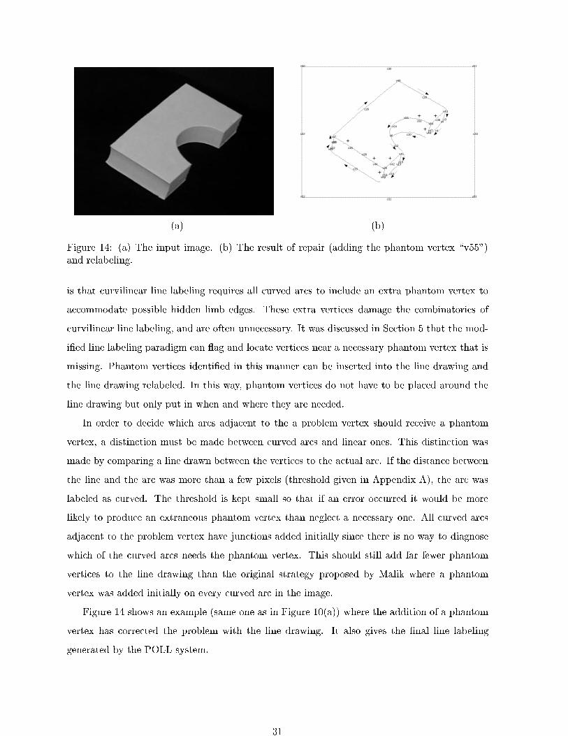
.................................................................................................................................................................................................................................................
....................
.....................................................
..............
..........................................................................................
....................
.............................
...................
..............................................
................................................................
....................
.............
.............
.........
..........
........
.........
.........
........
..........
..........
.........
.........
.........
.........
...........
..........
....
....
...
................
..............
..............
............
.......
.............
.................
.............
.............
............
............
............
............
.....
...................................................................................................................................................................................................................................................................................................................................................................................................................................................................................................................................................................................................................................................................................................................................................................................................................................................................................................................
...............
..............................................................................
v51
v53
v4
v43
v54
v44
v13
v49
v45
v6
v36
v46
v38
v20
v47
v48
v50
v52
v55
c33
c3c38
c4c47
c28
c15
c12
c10
c42
c16c53
c44
c26
c23
c45c22
c20
c30
c32
c31
c63
c64
+
+
+
+
+
++
(a) (b)
Figure 14: (a) The input image. (b) The result of repair (adding the phantom vertex \v55")and relabeling.
is that curvilinear line labeling requires all curved arcs to include an extra phantom vertex to
accommodate possible hidden limb edges. These extra vertices damage the combinatorics of
curvilinear line labeling, and are often unnecessary. It was discussed in Section 5 that the mod-
i�ed line labeling paradigm can ag and locate vertices near a necessary phantom vertex that is
missing. Phantom vertices identi�ed in this manner can be inserted into the line drawing and
the line drawing relabeled. In this way, phantom vertices do not have to be placed around the
line drawing but only put in when and where they are needed.
In order to decide which arcs adjacent to the a problem vertex should receive a phantom
vertex, a distinction must be made between curved arcs and linear ones. This distinction was
made by comparing a line drawn between the vertices to the actual arc. If the distance between
the line and the arc was more than a few pixels (threshold given in Appendix A), the arc was
labeled as curved. The threshold is kept small so that if an error occurred it would be more
likely to produce an extraneous phantom vertex than neglect a necessary one. All curved arcs
adjacent to the problem vertex have junctions added initially since there is no way to diagnose
which of the curved arcs needs the phantom vertex. This should still add far fewer phantom
vertices to the line drawing than the original strategy proposed by Malik where a phantom
vertex was added initially on every curved arc in the image.
Figure 14 shows an example (same one as in Figure 10(a)) where the addition of a phantom
vertex has corrected the problem with the line drawing. It also gives the �nal line labeling
generated by the POLL system.
31
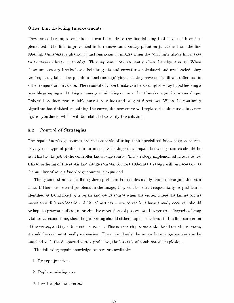
Other Line Labeling Improvements
There are other improvements that can be made to the line labeling that have not been im-
plemented. The �rst improvement is to remove unnecessary phantom junctions from the line
labeling. Unnecessary phantom junctions occur in images when the continuity algorithm makes
an extraneous break in an edge. This happens most frequently when the edge is noisy. When
these unnecessary breaks have their tangents and curvatures calculated and are labeled, they
are frequently labeled as phantom junctions signifying that they have no signi�cant di�erence in
either tangent or curvature. The removal of these breaks can be accomplished by hypothesizing a
possible grouping and �tting an energy minimizing curve without breaks to get its proper shape.
This will produce more reliable curvature values and tangent directions. When the continuity
algorithm has �nished smoothing the curve, the new curve will replace the old curves in a new
�gure hypothesis, which will be relabeled to verify the solution.
6.2 Control of Strategies
The repair knowledge sources are each capable of using their specialized knowledge to correct
exactly one type of problem in an image. Selecting which repair knowledge source should be
used �rst is the job of the controller knowledge source. The strategy implemented here is to use
a �xed ordering of the repair knowledge sources. A more elaborate strategy will be necessary as
the number of repair knowledge sources is expanded.
The general strategy for �xing these problems is to address only one problem junction at a
time. If there are several problems in the image, they will be solved sequentially. A problem is
identi�ed as being �xed by a repair knowledge source when the vertex where the failure occurs
moves to a di�erent location. A list of vertices where corrections have already occurred should
be kept to prevent endless, unproductive repetitions of processing. If a vertex is agged as being
a failure a second time, then the processing should either stop or backtrack to the �rst correction
of the vertex, and try a di�erent correction. This is a search process and, like all search processes,
it could be computationally expensive. The more closely the repair knowledge sources can be
matched with the diagnosed vertex problems, the less risk of combinatoric explosion.
The following repair knowledge sources are available:
1. Re-type junctions
2. Replace missing arcs
3. Insert a phantom vertex
32
4. Break a vertex into two vertices
5. Join two close vertices
6. Remove a phantom junction
There are two criteria for selecting the ordering of repair knowledge sources. Repair knowl-
edge sources that can be uniquely identi�ed, and are unlikely to be falsely triggered should be
used �rst. Repair knowledge sources that are risky, meaning that they could produce a correct
line labeling without correcting the real mistake(s) in the image, should be tried last.
An example of a repair knowledge source that can be uniquely identi�ed is the repair knowl-
edge source that breaks single vertices apart into two adjacent vertices. It can be uniquely
identi�ed by the presence of a junction with more than three incident arcs. Similarly the repair
knowledge source that groups proximate vertices together is well identi�ed by the presence of a
curve incident to one of the junctions that is much shorter than the other incident curves. These
knowledge sources should be tried �rst.
Risk is another consideration when ordering the repair knowledge sources. A repair knowl-
edge source is risky if it can make alterations that may produce a legal line labeling without
�xing the underlying problem in the image. In some sense, all of the repair knowledge sources
are risky, but two of them are particularly so: the repair knowledge source that inserts phantom
vertices and the repair knowledge source that replaces missing arcs. These strategies should be
tried as a last resort. Whether phantom vertices damage the combinatorics of line labeling has
not been established, but they certainly do not improve the combinatorics and are risky in the
sense that they relax an important constraint: that an arc may have one and only one label.
The risk in the knowledge source which inserts missing arcs can be limited by checking the arc
that gets inserted against the raw image data, to look for a subtle edge that the edge detection
algorithm may have missed, or using other constraints such as symmetry.
The repair knowledge source that re-types junctions is neither unique nor risky. It should
therefore be tried after the repair knowledge sources that break apart a vertex and joins close
vertices and before the repair knowledge source that inserts phantom junctions and missing
edges.
The only remaining repair knowledge source is the phantom vertex remover. Since it will
not be triggered falsely, it has no risk and can be run at anytime. In the interest of improving
the line drawing, it should be run �rst.
This gives the ordering used for triggering repair knowledge sources in the controller.
1. Remove a phantom vertex
33
2. Break a vertex into two vertices
3. Join two close vertices
4. Re-type junctions
5. Insert a phantom vertex
6. Replace missing arcs
As the number of implemented repair knowledge sources grows, more subtle strategies can be
developed for selecting among the choices. If a test set of images with ground truth is available,
an analysis could be done of the probability of each repair knowledge source �xing a problem
for each junction type. This type of experimentation could lead to a better understanding of
the frequency of each type of error and more sophisticated control strategies. The development
of insight into productive strategies was one of the purposes for using the blackboard paradigm.
7 Experimental Results
To test the system, the algorithms were run on the test bed of images shown in Appendix B.
We have assessed the performance of each part of the system (initial �gure units, line labeling
and diagnostics, and line labeling corrections) separately and each of these will be discussed in
this section.
The results of the performance of initial �gure hypothesis modules are summarized in Table 5.
Each of these mistakes is attributed to the module that caused the initial error. As an example,
an arrow junction might be missing an arc causing it to be seen as an L junction. This error would
be classi�ed as as missing edge and not a junction type failure since the junction classi�cation
is correct given the incorrect input. This system avoids double counting of errors.
There are eight di�erent mistakes that can be made by these four modules. There are two
errors that can occur in the weak membrane edge detection. The �rst is that edges can be
missing or broken, and the second is that extraneous edges can be found. The vertex proximity
module can make only two types of mistakes. Junctions that should have been grouped can
be separated, and junctions that should have been separated can be grouped. The continuity
module can make only two errors as well. Either an extra break can be added, or a corner can be
missed. The junction typing algorithm also has two types of errors. An error can be caused by
a mistake in tangents. Mistaking a three tangent junction for an arrow junction is an example
of this error. Mistakes in curvature can also cause errors. An example of this error is mistaking
a Curvature-L junction for an phantom junction.
34
In this set of images there are a total of 245 visible junctions and 323 visible arcs. There were
a total of 113 errors found in the initial processing, so the majority of the visible junctions and
arcs were properly processed. There was only one image with a perfect initial �gure hypothesis,
Image 8. There was also only one image with a very bad initial �gure hypothesis, Image 7.
The diÆculties in Image 7 arise on the right hand side of the background block. The rightmost
surface of this block is close to an accidental alignment and is therefore segmented into a large
number of small surfaces that these algorithms have diÆculty analyzing.
Appendix A shows the parameters that were used to calculate the initial �gure hypotheses.
Table 5 shows that the choice of parameters has balanced the errors. As an example, the value of
the vertex proximity threshold results in approximately the same number of junctions incorrectly
grouped (7) as broken (12). The same can be said for the continuity algorithm and the missing
(13) and extraneous breaks (13). The weak membrane edge detection is also creating roughly
the same number of extraneous edges (14) as missing edges (20).
The missing phantom junctions are not errors in the initial �gure hypothesis. In Malik's
line labeling paradigm [30], each curved arc was given a phantom junction. These phantom
junctions were not included in the initial �gure hypothesis because they can be detected from
line labeling failures and placed only at junctions where diÆculties arise.
One particular problem noticed in this processing was that all three tangent junctions were
mistaken for arrow junctions. Almost all of the curvature-L junctions were mistaken for L
junctions. This happens because �nding the curvature near junctions is diÆcult. This type of
problem can be ameliorated by the introduction of other modules such as shape from shading.
Separate research is currently under way to address this problem.
Examples of the results of the diagnostic line labeling module are at the end of Section 5. A
summary of the actual problems that exist in the test images is given in Table 6. Table 7 shows a
comparison between the faults that exist in the images and the ones that were diagnosed by the
algorithm. Multiple diagnoses for a single image were attained by manually correcting problems
as they were discovered to permit further problems to be diagnosed. Table 7 summarizes how
well the problems found in the initial �gure hypothesis have been detected by the modi�ed line
labeling paradigm using the oating object heuristic. Grouped junctions are easily detected
since having more than three arcs at a junction is not permitted within the object domain under
study in this paper.
Curvature and tangent mistakes in the classi�cation of the junctions are also found well.
The exception to this occurs when a pair of mistakes hide a problem. As an example, if a three
tangent junction is mistakenly identi�ed as an arrow and an adjacent curvature-L junction is also
35
mistaken for an L junction, then the mistake cannot be diagnosed since the labeling produced is
in fact legal in this object domain. In this case, the limb edge will be found to be a jump edge.
While this is unfortunate, it should be noted that both limb edges and jump edges represent
discontinuities of the scene depth and it is this similarity that permits confusion.
The mistakes that are the most diÆcult to diagnose are the missing breaks and extraneous
breaks in continuity. The diÆculty with diagnosis is that usually labelings both with or without
breaks are legal. Although the problem in these cases cannot be diagnosed, it should be noted
that the line labeling that is obtained is correct. In fact, the correctness of the line labeling
without regard to the placement of these breaks is what prevents proper diagnosis.
The localization of the diagnosis of problems in the �gure hypothesis is important. In almost
all of the cases reported in Table 6 the problem was diagnosed at the correct junction. In three
cases, the problem was diagnosed at an adjacent junction.
The modi�ed line labeling algorithm has been shown to be useful for identifying problems
in the initial line labeling hypothesis, although there are problems which cannot be diagnosed.
In all cases in the test bed of images, the junction that was diagnosed as being the problem was
either was the problem vertex, or was adjacent to the problem vertex.
Finally, we give the results of the corrections of the problems which were identi�ed by the
diagnostics of the line labeling problem. Table 8 gives a summary of the results from this module.
A comparison can be made between the problems that have been diagnosed in Section 5
and the problems that can be repaired using the repair knowledge sources. This comparison
is shown in Table 9. This table shows that most of the diagnosed problems can be �xed using
the repair knowledge sources. The extraneous edge problem that was not �xed was in image 7
where a near accidental alignment lead to an excessively cluttered area of the image. The overall
performance of this system in detecting correct line labelings will be discussed in Section 8.
Of the twenty-two images in the test bed given in Appendix B, one image could not be
labeled, one image had a convex edge mistaken for a limb, and �ve images had limb edges
mistaken for jump edges, and one image had a missing arc that wasn't replaced. Therefore
fourteen of the twenty-two images were processed completely correctly. Of the eight failures,
only one produced no line labeling. In the other seven failures, only one or two arcs were
mislabeled. Integration and diagnosis have dramatically improved the initial �gure hypotheses,
as can be seen in Table 10.
36
7.1 Execution Timings of Algorithms
The algorithms discussed in this paper were implemented in LISP, C, and Fortran on a Sparc-
server 690MP. The majority of the implementation was done in Allegro Common Lisp version
3.1.4, using the GBB blackboard system shell version 1.2. The LISP was compiled before tim-
ings were done. C was interfaced to Lisp to improve the execution speed of the numerical parts
of the program. Most array operations were implemented in C, as was the energy minimization
in the continuity algorithm. Fortran was only used for the program that performs the Voronoi
tesselation.
The run time of the edge detection, thinning and connected components algorithms are all
independent of the contents of the image, run times are given for one image (image 2 in the test
set in Appendix B). The weak membrane edge detection ran in 214 seconds (3.5 minutes). The
thinning took .7 seconds. The connected components algorithm took 10.4 seconds. The longest
time it took to process an image and generate a labeled line drawing after weak membrane edge
detection, thinning, and connected components had been performed was 14.6 minutes on image
20. The run times of these algorithms were found using the time command in Lisp. All times
exclude garbage collection.
8 Conclusions
This paper described the POLL system for obtaining labeled line drawings from single intensity
images using an integrated system. The goal of this research was to demonstrate that even when
individual visual processing modules are not very robust, one can increase the robustness and
quality of the overall system and 3D interpretation by integrating a collection of such modules.
In particular, the POLL system has demonstrated the following capabilities:
1. One can obtain 3D interpretations of real images (single intensity images) in the form of
labeled line drawings.
2. This system is unique in that it uses piecewise smooth objects, instead of the more restric-
tive planar or quadric surface models that are often used, particularly in range imagery
as in [62, 35]. This enhances the generality of the system, but also greatly increases the
diÆculty of the problem.
3. This result is achieved through the integration of the following modules: edge detection,
region segmentation, curvilinear grouping, and line labeling.
4. In the cases where an unambiguous labeling cannot be extracted, the POLL system will
37
produce partial results. These partial results can be further re�ned and disambiguated
as other modules are added and further interpretations can be done. Examples of such
modules can be shape from shading, stereo, etc.
5. The POLL system has demonstrated that the blackboard systems are useful platforms for
integrating di�erent visual modules with diverse representations.
6. The system also works without reference to a set of object models. This distinguishes the
system from e�orts like the Schema blackboard system [37], where object models were
extensively used.
One of the shortcomings of the POLL system is that it does require objects to have smooth
surfaces with no markings and texture. This is a direct result of the curvilinear line labeling
scheme used to interpret the line drawings. Future research will look into the integration of
modules that can process such objects. The shape from shading and symmetry detection can
be incorporated in the future which would improve the results. The problem of adding shape
from shading and stereo modules to this scheme is being studied independently and the initial
results in terms of the ability to distinguish limb edges from jump edges are encouranging [63].
Other modules that could be added are surface �tting modules which would guide the 3D
interpretation process more robustly.
A Parameters
Many of the modules and algorithms used in this paper have parameters. These parameters
were set empirically, after experimentation with the test bed of images which will be shown in
Appendix B. In order to make this work reproducable, all of the parameters used are given in
this appendix. The parameters are in the order of �rst discussion.
Section 3.2 states that the continuity grouping algorithm of Trytten and Tuceryan [21] is
used to perform the curvilinear grouping. The parameters for this algorithm fall into three
categories: parameters for the energy formulation, parameters for Canny edge detection, and
the multi-grid relaxation parameters. These parameters and their physical interpretations are
summarized in Table 11.
38
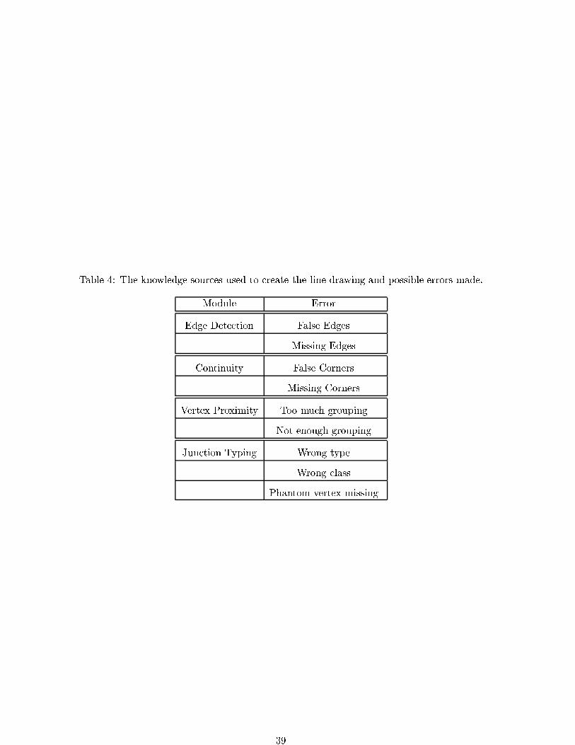
Table 4: The knowledge sources used to create the line drawing and possible errors made.
Module Error
Edge Detection False Edges
Missing Edges
Continuity False Corners
Missing Corners
Vertex Proximity Too much grouping
Not enough grouping
Junction Typing Wrong type
Wrong class
Phantom vertex missing
39
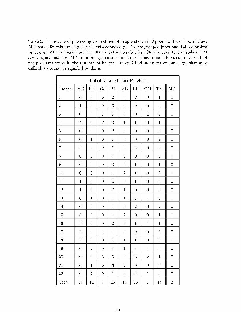
Table 5: The results of processing the test bed of images shown in Appendix B are shown below.ME stands for missing edges. EE is extraneous edges. GJ are grouped junctions. BJ are brokenjunctions. MB are missed breaks. EB are extraneous breaks. CM are curvature mistakes. TMare tangent mistakes. MP are missing phantom junctions. These nine failures summarize all ofthe problems found in the test bed of images. Image 7 had many extraneous edges that werediÆcult to count, as signi�ed by the a.
Initial Line Labeling Problems
Image ME EE GJ BJ MB EB CM TM MP
1 0 0 0 0 0 2 0 1 1
2 1 0 0 0 0 0 0 0 0
3 0 0 1 0 0 0 1 2 0
4 4 0 2 0 1 1 0 1 0
5 0 0 0 2 0 0 0 0 0
6 0 1 0 0 0 0 0 2 0
7 2 a 0 1 0 3 0 0 0
8 0 0 0 0 0 0 0 0 0
9 0 0 0 0 0 1 0 1 0
10 0 0 0 1 2 1 0 2 0
11 1 0 0 0 0 1 0 0 0
12 1 0 0 0 1 0 0 0 0
13 0 1 0 0 1 3 1 0 0
14 0 0 0 1 0 2 0 2 0
15 3 0 0 1 2 0 0 1 0
16 3 0 0 0 0 1 1 1 0
17 2 0 1 1 2 0 0 2 0
18 3 0 0 1 1 1 0 0 1
19 0 2 0 1 1 3 1 0 0
20 0 2 3 0 0 3 2 1 0
21 0 1 0 3 2 0 0 0 0
22 0 7 0 1 0 4 1 0 0
Total 20 14 7 13 13 26 7 16 2
40
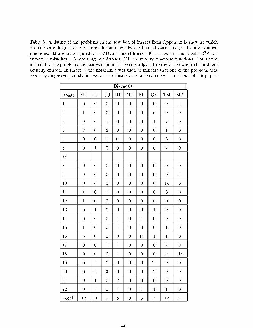
Table 6: A listing of the problems in the test bed of images from Appendix B showing whichproblems are diagnosed. ME stands for missing edges. EE is extraneous edges. GJ are groupedjunctions. BJ are broken junctions. MB are missed breaks. EB are extraneous breaks. CM arecurvature mistakes. TM are tangent mistakes. MP are missing phantom junctions. Notation ameans that the problem diagnosis was found at a vertex adjacent to the vertex where the problemactually existed. In Image 7, the notation b was used to indicate that one of the problems wascorrectly diagnosed, but the image was too cluttered to be �xed using the methods of this paper.
Diagnosis
Image ME EE GJ BJ MB EB CM TM MP
1 0 0 0 0 0 0 0 0 1
2 1 0 0 0 0 0 0 0 0
3 0 0 1 0 0 0 1 2 0
4 3 0 2 0 0 0 0 1 0
5 0 0 0 1a 0 0 0 0 0
6 0 1 0 0 0 0 0 2 0
7b
8 0 0 0 0 0 0 0 0 0
9 0 0 0 0 0 0 b 0 1
10 0 0 0 0 0 0 0 1a 0
11 1 0 0 0 0 0 0 0 0
12 1 0 0 0 0 0 0 0 0
13 0 1 0 0 0 0 1 0 0
14 0 0 0 1 0 1 0 0 0
15 1 0 0 1 0 0 0 1 0
16 3 0 0 0 0 1a 1 1 0
17 0 0 1 1 0 0 0 2 0
18 2 0 0 1 0 0 0 0 1a
19 0 3 0 0 0 0 1a 0 0
20 0 2 3 0 0 0 2 0 0
21 0 1 0 2 0 0 0 0 0
22 0 3 0 1 0 1 1 1 0
Total 12 11 7 8 0 3 7 12 2
41

Table 7: A comparison between the faults in the images from Table 5, and the problems thatwere diagnosed using the oating object heuristic.
Source ME EE GJ BJ MB EB CM TM MP
Initial 20 14 7 13 13 26 7 16 2
Diagnosed 12 11 7 8 0 3 7 11 2
42
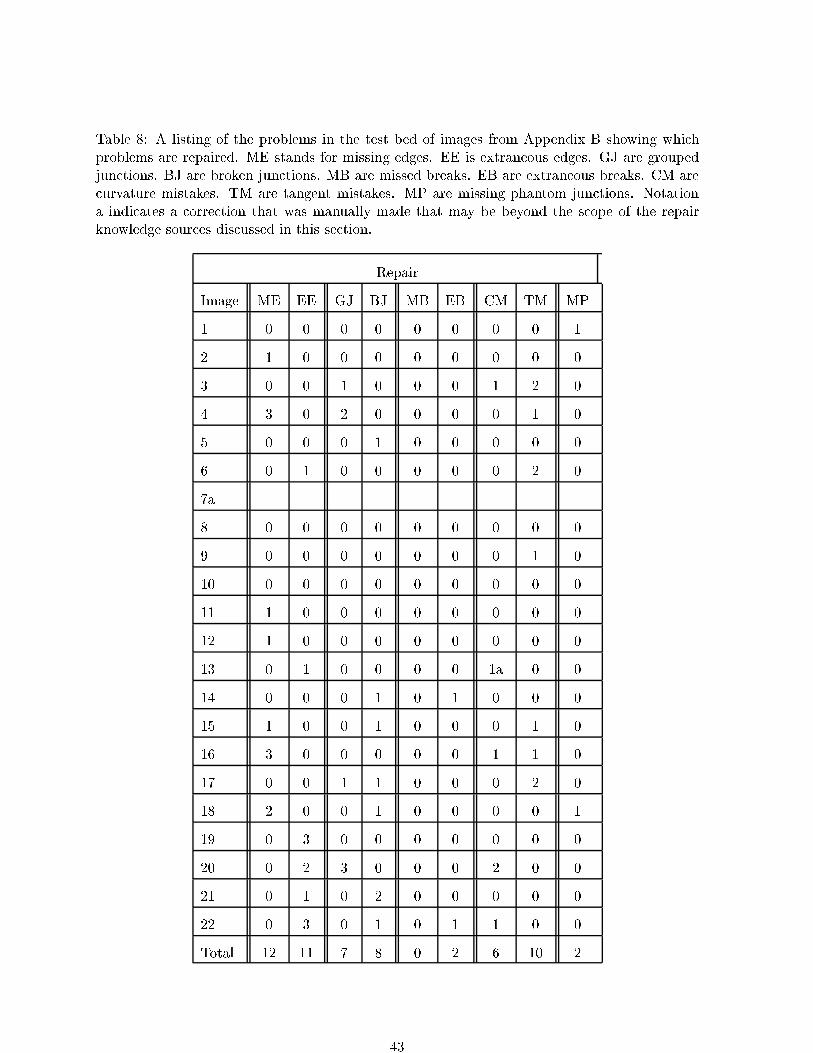
Table 8: A listing of the problems in the test bed of images from Appendix B showing whichproblems are repaired. ME stands for missing edges. EE is extraneous edges. GJ are groupedjunctions. BJ are broken junctions. MB are missed breaks. EB are extraneous breaks. CM arecurvature mistakes. TM are tangent mistakes. MP are missing phantom junctions. Notationa indicates a correction that was manually made that may be beyond the scope of the repairknowledge sources discussed in this section.
Repair
Image ME EE GJ BJ MB EB CM TM MP
1 0 0 0 0 0 0 0 0 1
2 1 0 0 0 0 0 0 0 0
3 0 0 1 0 0 0 1 2 0
4 3 0 2 0 0 0 0 1 0
5 0 0 0 1 0 0 0 0 0
6 0 1 0 0 0 0 0 2 0
7a
8 0 0 0 0 0 0 0 0 0
9 0 0 0 0 0 0 0 1 0
10 0 0 0 0 0 0 0 0 0
11 1 0 0 0 0 0 0 0 0
12 1 0 0 0 0 0 0 0 0
13 0 1 0 0 0 0 1a 0 0
14 0 0 0 1 0 1 0 0 0
15 1 0 0 1 0 0 0 1 0
16 3 0 0 0 0 0 1 1 0
17 0 0 1 1 0 0 0 2 0
18 2 0 0 1 0 0 0 0 1
19 0 3 0 0 0 0 0 0 0
20 0 2 3 0 0 0 2 0 0
21 0 1 0 2 0 0 0 0 0
22 0 3 0 1 0 1 1 0 0
Total 12 11 7 8 0 2 6 10 2
43
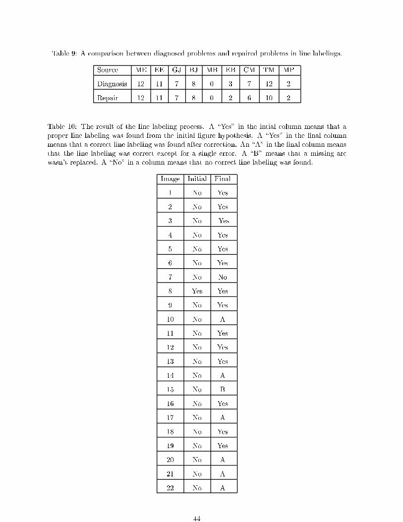
Table 9: A comparison between diagnosed problems and repaired problems in line labelings.
Source ME EE GJ BJ MB EB CM TM MP
Diagnosis 12 11 7 8 0 3 7 12 2
Repair 12 11 7 8 0 2 6 10 2
Table 10: The result of the line labeling process. A \Yes" in the intial column means that aproper line labeling was found from the initial �gure hypothesis. A \Yes" in the �nal columnmeans that a correct line labeling was found after correction. An \A" in the �nal column meansthat the line labeling was correct except for a single error. A \B" means that a missing arcwasn't replaced. A \No" in a column means that no correct line labeling was found.
Image Initial Final
1 No Yes
2 No Yes
3 No Yes
4 No Yes
5 No Yes
6 No Yes
7 No No
8 Yes Yes
9 No Yes
10 No A
11 No Yes
12 No Yes
13 No Yes
14 No A
15 No B
16 No Yes
17 No A
18 No Yes
19 No Yes
20 No A
21 No A
22 No A
44
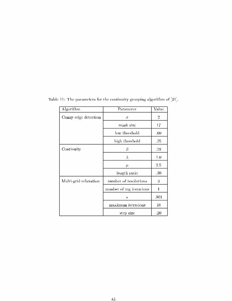
Table 11: The parameters for the continuity grouping algorithm of [21].
Algorithm Parameter Value
Canny edge detection � 2
mask size 17
low threshold .60
high threshold .75
Continuity � .28
� 1.0
� 2.5
length ratio .30
Multi-grid relaxation number of resolutions 3
number of mg iterations 1
� .001
maximum iterations 10
step size .20
45
In Section 4.2.1, edge detection was performed using the weak membrane edge model and
the GNC algorithm for energy minimization. The parameters for the edge detection are shown
in Table 12. Curve hypotheses were created for the boundary of regions that were suÆciently
large, the speci�c numerical de�nition of large is given in Table 12. Edgels that were too short
were removed from consideration. The parameter for this is also given in Table 12.
Section 4.2.2 also used a variety of parameters. The circular arc �tting parameters were used
to determine how many pixels near the endpoint of a curve should be used for approximating
the curvature and tangent direction. The curvature values were found to be unreliable, and
were assigned to three classes: straight, curved and very curved. These symbolic curvatures
were used in all comparisons.
In Section 6.1, a parameter for the number of pixels that separate a line from an arc is
discussed. The value for this parameter is three pixels.
B Test Bed of Images
The POLL system was tested on twenty-two intensity images captured using a Macintosh II-FX
in the PRIP Laboratory of Michigan State University. These images are labeled and shown in
Figure 15, Figure 16, Figure 17, and Figure 18. Most of the side surfaces of the bath tub toys
used in Images 1 to 18 have shrunk and are slightly curved.
46
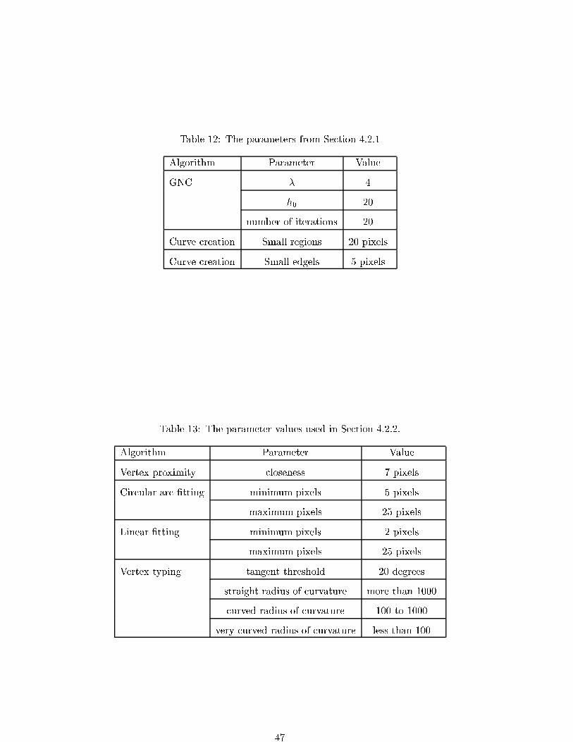
Table 12: The parameters from Section 4.2.1
Algorithm Parameter Value
GNC � 4
h0 20
number of iterations 20
Curve creation Small regions 20 pixels
Curve creation Small edgels 5 pixels
Table 13: The parameter values used in Section 4.2.2.
Algorithm Parameter Value
Vertex proximity closeness 7 pixels
Circular arc �tting minimum pixels 5 pixels
maximum pixels 25 pixels
Linear �tting minimum pixels 2 pixels
maximum pixels 25 pixels
Vertex typing tangent threshold 20 degrees
straight radius of curvature more than 1000
curved radius of curvature 100 to 1000
very curved radius of curvature less than 100
47
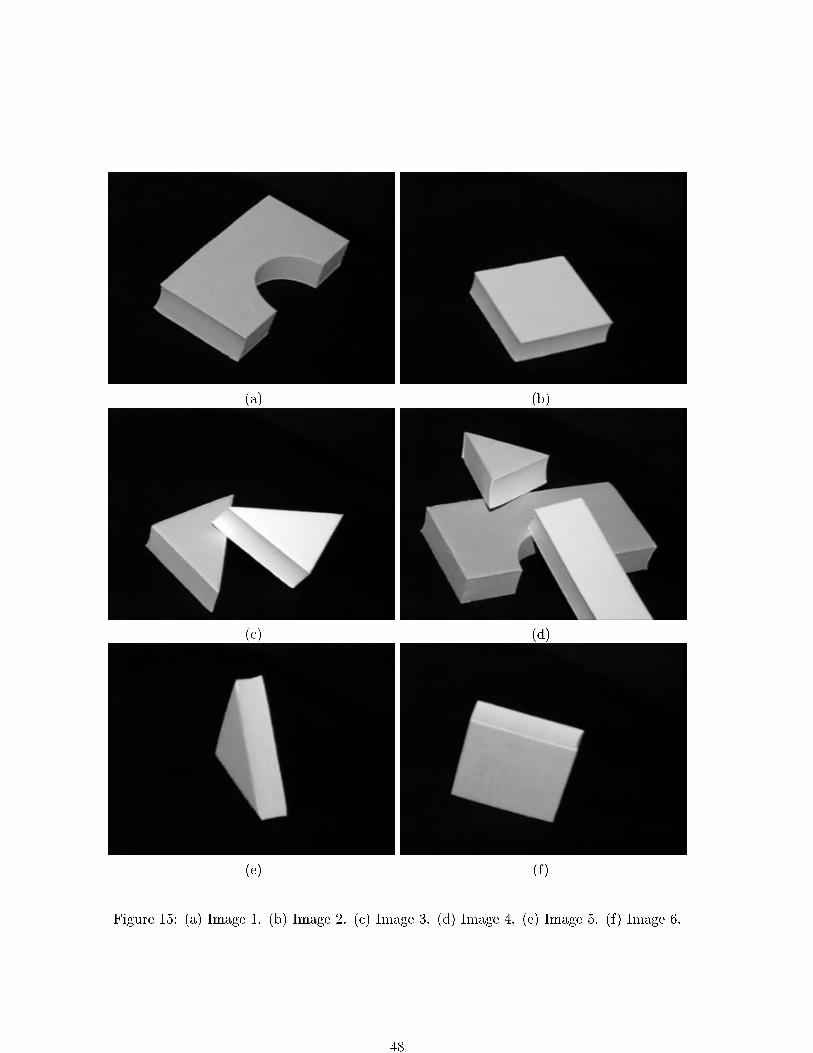
(a) (b)
(c) (d)
(e) (f)
Figure 15: (a) Image 1. (b) Image 2. (c) Image 3. (d) Image 4. (e) Image 5. (f) Image 6.
48
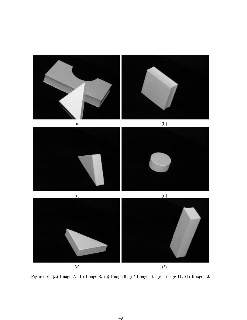
(a) (b)
(c) (d)
(e) (f)
Figure 16: (a) Image 7. (b) Image 8. (c) Image 9. (d) Image 10. (e) Image 11. (f) Image 12.
49
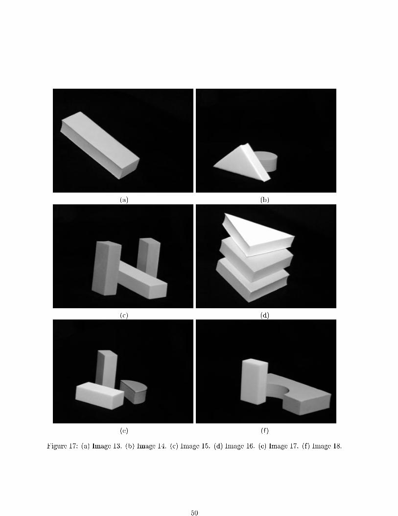
(a) (b)
(c) (d)
(e) (f)
Figure 17: (a) Image 13. (b) Image 14. (c) Image 15. (d) Image 16. (e) Image 17. (f) Image 18.
50
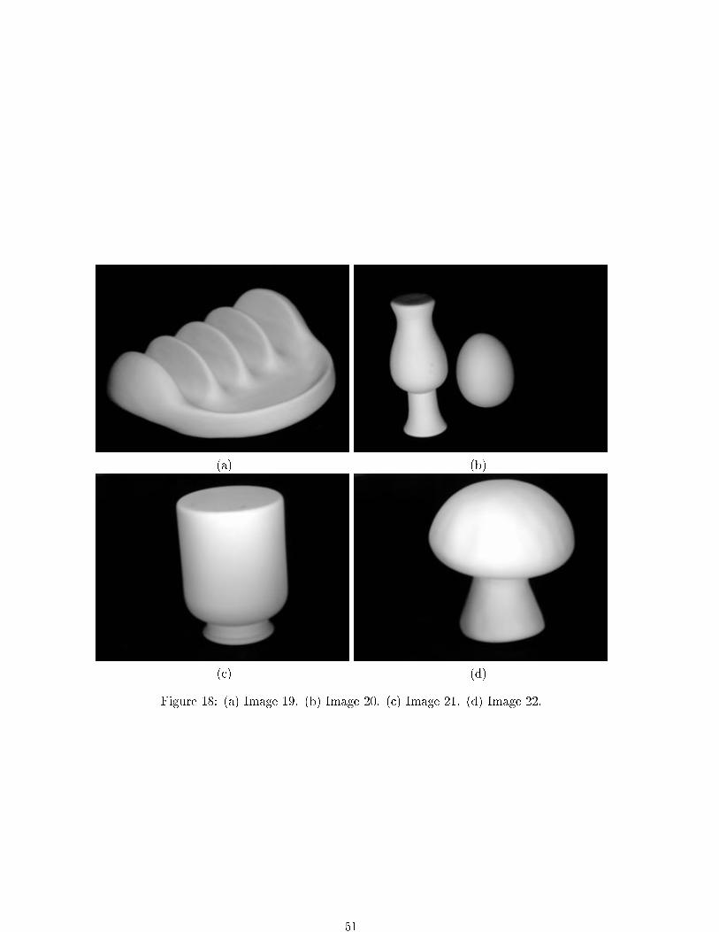
(a) (b)
(c) (d)
Figure 18: (a) Image 19. (b) Image 20. (c) Image 21. (d) Image 22.
51
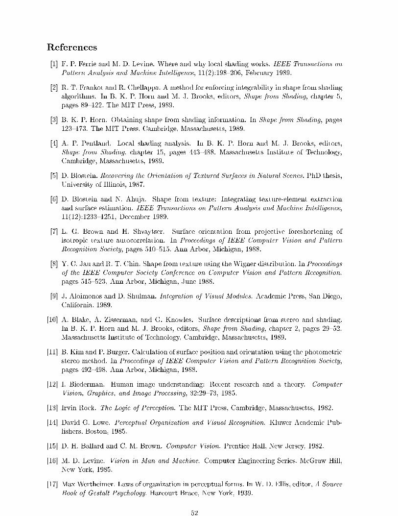
References
[1] F. P. Ferrie and M. D. Levine. Where and why local shading works. IEEE Transactions on
Pattern Analysis and Machine Intelligence, 11(2):198{206, February 1989.
[2] R. T. Frankot and R. Chellappa. A method for enforcing integrability in shape from shadingalgorithms. In B. K. P. Horn and M. J. Brooks, editors, Shape from Shading, chapter 5,pages 89{122. The MIT Press, 1989.
[3] B. K. P. Horn. Obtaining shape from shading information. In Shape from Shading, pages123{173. The MIT Press, Cambridge, Massachusetts, 1989.
[4] A. P. Pentland. Local shading analysis. In B. K. P. Horn and M. J. Brooks, editors,Shape from Shading, chapter 15, pages 443{488. Massachusetts Institute of Technology,Cambridge, Massachusetts, 1989.
[5] D. Blostein. Recovering the Orientation of Textured Surfaces in Natural Scenes. PhD thesis,University of Illinois, 1987.
[6] D. Blostein and N. Ahuja. Shape from texture: Integrating texture-element extractionand surface estimation. IEEE Transactions on Pattern Analysis and Machine Intelligence,11(12):1233{1251, December 1989.
[7] L. G. Brown and H. Shvaytser. Surface orientation from projective foreshortening ofisotropic texture autocorrelation. In Proceedings of IEEE Computer Vision and Pattern
Recognition Society, pages 510{515, Ann Arbor, Michigan, 1988.
[8] Y. C. Jau and R. T. Chin. Shape from texture using the Wigner distribution. In Proceedingsof the IEEE Computer Society Conference on Computer Vision and Pattern Recognition,pages 515{523, Ann Arbor, Michigan, June 1988.
[9] J. Aloimonos and D. Shulman. Integration of Visual Modules. Academic Press, San Diego,California, 1989.
[10] A. Blake, A. Zisserman, and G. Knowles. Surface descriptions from stereo and shading.In B. K. P. Horn and M. J. Brooks, editors, Shape from Shading, chapter 2, pages 29{52.Massachusetts Institute of Technology, Cambridge, Massachusetts, 1989.
[11] B. Kim and P. Burger. Calculation of surface position and orientation using the photometricstereo method. In Proceedings of IEEE Computer Vision and Pattern Recognition Society,pages 492{498, Ann Arbor, Michigan, 1988.
[12] I. Biederman. Human image understanding: Recent research and a theory. Computer
Vision, Graphics, and Image Processing, 32:29{73, 1985.
[13] Irvin Rock. The Logic of Perception. The MIT Press, Cambridge, Massachusetts, 1982.
[14] David G. Lowe. Perceptual Organization and Visual Recognition. Kluwer Academic Pub-lishers, Boston, 1985.
[15] D. H. Ballard and C. M. Brown. Computer Vision. Prentice Hall, New Jersey, 1982.
[16] M. D. Levine. Vision in Man and Machine. Computer Engineering Series. McGraw Hill,New York, 1985.
[17] Max Wertheimer. Laws of organization in perceptual forms. In W. D. Ellis, editor, A Source
Book of Gestalt Psychology. Harcourt Brace, New York, 1939.
52
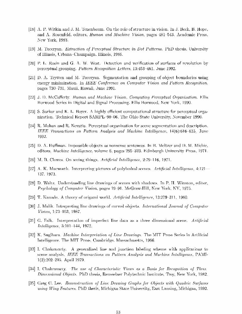
[18] A. P. Witkin and J. M. Tenenbaum. On the role of structure in vision. In J. Beck, B. Hope,and A. Rosenfeld, editors, Human and Machine Vision, pages 481{543. Academic Press,New York, 1983.
[19] M. Tuceryan. Extraction of Perceptual Structure in Dot Patterns. PhD thesis, Universityof Illinois, Urbana{Champaign, Illinois, 1986.
[20] P. L. Rosin and G. A. W. West. Detection and veri�cation of surfaces of revolution byperceptual grouping. Pattern Recognition Letters, 13:453{461, June 1992.
[21] D. A. Trytten and M. Tuceryan. Segmentation and grouping of object boundaries usingenergy minimization. In IEEE Conference on Computer Vision and Pattern Recognition,pages 730{731, Mauii, Hawaii, June 1991.
[22] J. D. McCa�erty. Human and Machine Vision, Computing Perceptual Organization. EllisHorwood Series in Digital and Signal Processing. Ellis Horwood, New York, 1990.
[23] S. Sarkar and K. L. Boyer. A highly eÆcient computational structure for perceptual orga-nization. Technical Report SAMPL{90{06, The Ohio State University, November 1990.
[24] R. Mohan and R. Nevatia. Perceptual organization for scene segmentation and description.IEEE Transactions on Pattern Analysis and Machine Intelligence, 14(6):616{635, June1992.
[25] D. A. Hu�man. Impossible objects as nonsense sentences. In B. Meltzer and D. M. Michie,editors, Machine Intelligence, volume 6, pages 295{323. Edinburgh University Press, 1971.
[26] M. B. Clowes. On seeing things. Arti�cial Intelligence, 2:79{116, 1971.
[27] A. K. Macworth. Interpreting pictures of polyhedral scenes. Arti�cial Intelligence, 4:121{137, 1973.
[28] D. Waltz. Understanding line drawings of scenes with shadows. In P. H. Winston, editor,Psychology of Computer Vision, pages 19{91. McGraw-Hill, New York, NY, 1975.
[29] T. Kanade. A theory of origami world. Arti�cial Intelligence, 13:279{311, 1980.
[30] J. Malik. Interpreting line drawings of curved objects. International Journal of ComputerVision, 1:73{103, 1987.
[31] G. Falk. Interpretation of imperfect line data as a three dimensional scene. Arti�cial
Intelligence, 3:101{144, 1972.
[32] K. Sugihara. Machine Interpretation of Line Drawings. The MIT Press Series in Arti�cialIntelligence. The MIT Press, Cambridge, Massachusetts, 1986.
[33] I. Chakravarty. A generalized line and junction labeling scheme with applications toscene analysis. IEEE Transactions on Pattern Analysis and Machine Intelligence, PAMI-1(2):202{205, April 1979.
[34] I. Chakravarty. The use of Characteristic Views as a Basis for Recognition of Three-
Dimensional Objects. PhD thesis, Rensselaer Polytechnic Institute, Troy, New York, 1982.
[35] Greg C. Lee. Reconstruction of Line Drawing Graphs for Objects with Quadric Surfaces
using Wing Features. PhD thesis, Michigan State University, East Lansing, Michigan, 1992.
53
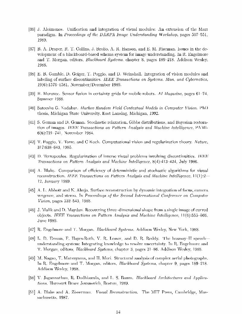
[36] J. Aloimonos. Uni�cation and integration of visual modules: An extension of the Marrparadigm. In Proceedings of the DARPA Image Understanding Workshop, pages 507{551,1989.
[37] B. A. Draper, R. T. Collins, J. Brolio, A. R. Hanson, and E. M. Riseman. Issues in the de-velopment of a blackboard-based schema system for image understanding. In R. Engelmoreand T. Morgan, editors, Blackboard Systems, chapter 8, pages 189{218. Addison Wesley,1988.
[38] E. B. Gamble, D. Geiger, T. Poggio, and D. Weinshall. Integration of vision modules andlabeling of surface discontinuities. IEEE Transactions on Systems, Man, and Cybernetics,19(6):1576{1581, November/December 1989.
[39] H. Moravec. Sensor fusion in certainty grids for mobile robots. AI Magazine, pages 61{74,Summer 1988.
[40] Sateesha G. Nadabar. Markov Random Field Contextual Models in Computer Vision. PhDthesis, Michigan State University, East Lansing, Michigan, 1992.
[41] S. Geman and D. Geman. Stochastic relaxation, Gibbs distributions, and Bayesian restora-tion of images. IEEE Transactions on Pattern Analysis and Machine Intelligence, PAMI-6(6):721{741, November 1984.
[42] T. Poggio, V. Torre, and C Koch. Computational vision and regularization theory. Nature,317:638{643, 1985.
[43] D. Terzopoulos. Regularization of inverse visual problems involving discontinuities. IEEETransactions on Pattern Analysis and Machine Intelligence, 8(4):413{424, July 1986.
[44] A. Blake. Comparison of eÆciency of deterministic and stochastic algorithms for visualreconstruction. IEEE Transactions on Pattern Analysis and Machine Intelligence, 11(1):2{12, January 1989.
[45] A. L. Abbott and N. Ahuja. Surface reconstruction by dynamic integration of focus, cameravergence, and stereo. In Proceedings of the Second International Conference on Computer
Vision, pages 532{543, 1988.
[46] J. Malik and D. Maydan. Recovering three{dimensional shape from a single image of curvedobjects. IEEE Transactions on Pattern Analysis and Machine Intelligence, 11(6):555{566,June 1989.
[47] R. Engelmore and T. Morgan. Blackboard Systems. Addison Wesley, New York, 1988.
[48] L. D. Erman, F. Hayes-Roth, V. R. Lesser, and D. R. Reddy. The hearsay{II speech{understanding system: Integrating knowledge to resolve uncertainty. In R. Engelmore andT. Morgan, editors, Blackboard Systems, chapter 3, pages 31{86. Addison Wesley, 1988.
[49] M. Nagao, T. Matsuyama, and H. Mori. Structural analysis of complex aerial photographs.In R. Engelmore and T. Morgan, editors, Blackboard Systems, chapter 9, pages 189{218.Addison Wesley, 1988.
[50] V. Jagannathan, R. Dodhiawala, and L. S. Baum. Blackboard Architectures and Applica-
tions. Harcourt Brace Jovanovich, Boston, 1989.
[51] A. Blake and A. Zisserman. Visual Reconstruction. The MIT Press, Cambridge, Mas-sachusetts, 1987.
54
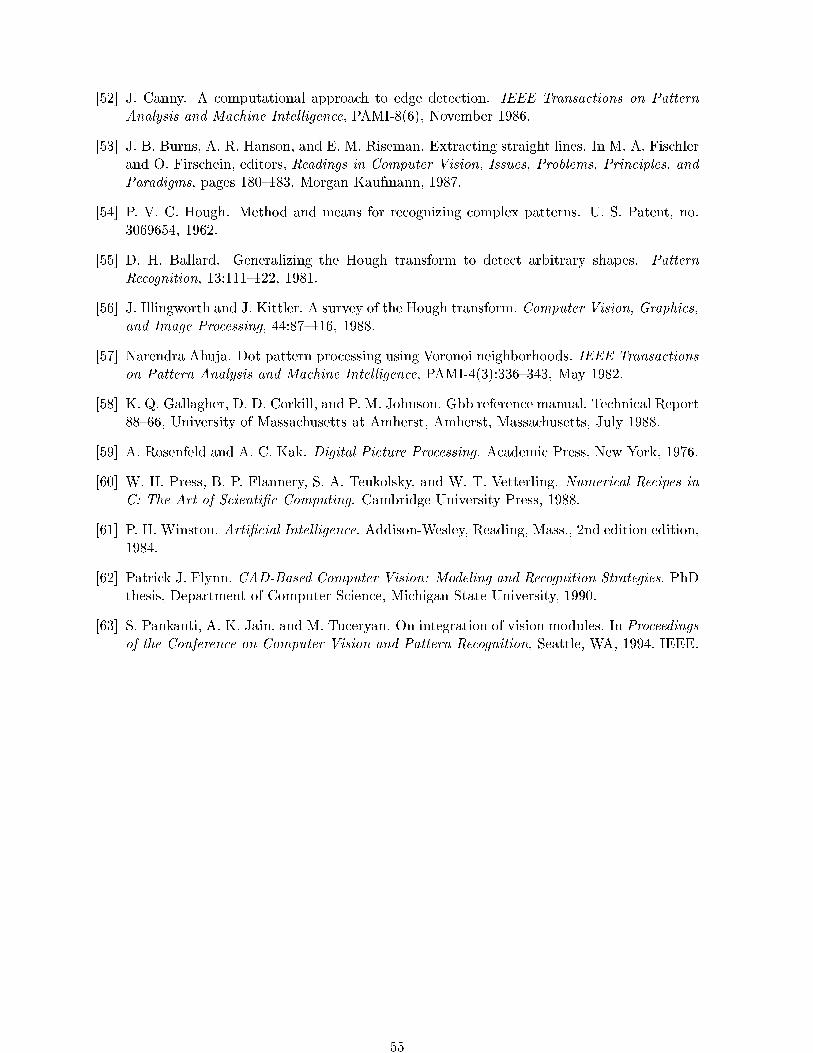
[52] J. Canny. A computational approach to edge detection. IEEE Transactions on Pattern
Analysis and Machine Intelligence, PAMI-8(6), November 1986.
[53] J. B. Burns, A. R. Hanson, and E. M. Riseman. Extracting straight lines. In M. A. Fischlerand O. Firschein, editors, Readings in Computer Vision, Issues, Problems, Principles, and
Paradigms, pages 180{183. Morgan Kaufmann, 1987.
[54] P. V. C. Hough. Method and means for recognizing complex patterns. U. S. Patent, no.3069654, 1962.
[55] D. H. Ballard. Generalizing the Hough transform to detect arbitrary shapes. Pattern
Recognition, 13:111{122, 1981.
[56] J. Illingworth and J. Kittler. A survey of the Hough transform. Computer Vision, Graphics,and Image Processing, 44:87{116, 1988.
[57] Narendra Ahuja. Dot pattern processing using Voronoi neighborhoods. IEEE Transactions
on Pattern Analysis and Machine Intelligence, PAMI-4(3):336{343, May 1982.
[58] K. Q. Gallagher, D. D. Corkill, and P. M. Johnson. Gbb reference manual. Technical Report88{66, University of Massachusetts at Amherst, Amherst, Massachusetts, July 1988.
[59] A. Rosenfeld and A. C. Kak. Digital Picture Processing. Academic Press, New York, 1976.
[60] W. H. Press, B. P. Flannery, S. A. Teukolsky, and W. T. Vetterling. Numerical Recipes inC: The Art of Scienti�c Computing. Cambridge University Press, 1988.
[61] P. H. Winston. Arti�cial Intelligence. Addison-Wesley, Reading, Mass., 2nd edition edition,1984.
[62] Patrick J. Flynn. CAD-Based Computer Vision: Modeling and Recognition Strategies. PhDthesis, Department of Computer Science, Michigan State University, 1990.
[63] S. Pankanti, A. K. Jain, and M. Tuceryan. On integration of vision modules. In Proceedingsof the Conference on Computer Vision and Pattern Recognition, Seattle, WA, 1994. IEEE.
55


