Journal of Educational Measurement Spring 2004, Vol. 41, No. 1, pp. 1.5-32

The Chain and Post-Stratification Methods for Observed-Score Equating:

Their Relationship to Population Invariance

A h a A. von Davier, Paul W. Holland, and Dorothy T. Thayer Educational Testing Service, Princeton, NJ

The Norz-Equivalent-groups Anchor Test (NEAT) design has been in wide use since at least the early 1940s. It involves two populations of test takers, P and Q, and makes use of an anchor test to link them. Two linking methods used for NEAT designs ure those ( a ) based on chain quating and (b) that use the anchor test to post-strati& the distributions of the two operational test scores to a common population (i.e., Tucker equating and frequency estimation). We show that, under digwent sets of assumptions, both methods are observed score equuting methods and we give conditions under which the methods give identical results. In addition, we develop analogues of the Doratis and Holland (2000) RMSD measures of population invariance of equating methods for the NEAT design,for both chain and Vost-stratification equating methods.

1. Introduction Test cquating methods are used to produce scores that are comparable across

different test forms. Weaker forms of test linking often use the same computations as test cquating but do not necessarily result in scores that are comparable. One of the five requirements of equating functions identified in Dorans and Holland (2000) is that equating should be population invariant. Because strict population invariance is oftcn impossible to achieve, Dorans and Holland (2000) introduced a measure of the degree to which an equating function is sensitive to the population on which it is computed. The measure compares equating or linking functions computed on different subpopulations with the equating or linking function computed for the whole population. Their discussion is restricted to equating designs that involve only one population, such as the equivalent-groups and the single-group designs.

The Non-Equivalent-groups Anchor Test (NEAT) design involves two popula- tions of test takers, P and Q (usually different test administrations), and makes use of an anchor test to link them. We also want population invariance to hold for equating functions used in the NEAT design, but there are two populations in the NEAT design, and there can be ambiguity as to the population on which the equating (or linking) is done.

For the NEAT design there are several observed-score equating (OSE) methods that are used in practice. Two important classes of these methods are those we call chain equating (CE) and those we call post-stratification equating (PSE). We define these methods more carefully in Section 3.

In this article we examine the relationship of CE versus PSE methods in the NEAT design from the following points of view:

15

von Davies Holland, and Thayer

1. We show that both are examples of OSE methods under different assumptions that are usually untestable.

2. We give (idealized) conditions under which both methods produce the same equating function.

3. We generalize the Dorans and Holland (2000) RMSD measures of the popula- tion invariance of equating and linking functions to the case of the NEAT design for both CE and PSE methods.

2. Observed Score Equating and the NEAT Design

We assume there are two tests to be equated, X and Y, and a “target” population, Ton which this is to be done. The target population that is relevant will depend on the equating design used (Braun & Holland, 1982; Kolen & Brennan, 1995). Many OSE methods and methods of test linking are based on the equipercentile equating function. It is defined on the target population, T, as:

(1) where FAX) and C&) are the cumulative distribution functions (CDFs), of X and Y, respectively, on T. In order for this definition to make sense we also assume that FAX) and G&) have been made continuous or “continuized” so that the inverse functions exist for F,(x) and G,(J). (See Appendix €3 for an outline of kernel equating where continuization is considered as an explicit step in the equating process.)

exu,&) = G, ‘ (FAX)) = G, ‘oF&x),

2.1 The Linear and Equipercentile Equating Functions

The two most common OSE functions are the linear and equipercentile-equating functions on T. These are sometimes viewed as different methods, but Theorem 1 (below) summarizes the close relationship that they share. The linear equating function, LinXy+), is defined by

(2) Lin,,,(x) = Pn. + u,((x - PXJUX, ) .

The equipercentile equating function, exy;&) is defined in Equation 1. Theorem 1: For any population, T, exu;.,(x) = Lin,,&) + R(x), where

R(x) = u&(x - pXr)/(rxT), and E(U) = G,j ‘oF,(u) - u. (3 Fo(u) and Go(u) are CDFs with mean zero and variance one that satisfy the equations:

FAX) = Fo((x - ~xT)/uxT), GAY) = CO((Y - ~m)/uyr). (4) (Note that Theorem 1 presumes that the continuization process has preserved the first two moments of X and Yon T.)

In Theorem 1, the remainder, R(x), is the non-linear part of the equipercentile equating function. When F,(u) and G,(u) are the same, ~(x), and, therefore, R(>x), is identically 0 so that exy;.7(x) = Lin,,&). The details of the proof of Theorem 1 are straightforward and discussed in von Davier, Holland, and Thayer (2004).

16

Chain and Pr,st-Strati~catiori Equating Methods

2.2 The NEAT Design

The NEAT design is very common. The two “operational tests” to be equated, X and Y, arc given to two samples of examines from different test populations or “administrations” (denoted here by the populations P and Q). Ln addition, an anchor test, V, is given to both samples from P and Q resulting in the following data structure, where d denotes the presence of data.

X V Y

P v v X , V observed on P, ( 5 ) (2 J v v Y, Vobserved on (2.

The anchor test score, V , can be either a part of both X and Y (the internal anchor case) or a separate score (the external anchor case).

The Target Population, T, for the NEAT design is a mixture of P and Q in which P and Q are regarded as partitioning T, P and Q, are also given weights that sum to 1. This is denoted by

T = w P + ( l - w ) Q . (6)

The partition of T is determined by the weight w. If w = 1, then T = P and if w = 0 then T = Q. If w = %, then P and Q are represented equally in T. Any choice of w between 0 and I is possible, and reflects the amount of weight that is given to P and Q in determining the target population. Not every population can be repre- sented as a weighted partition. In particular, any proper subpopulation of P or of Q is not a mixture of P and Q of the form given in Equation 6.

A mixture can be thought of as a pooling of the data observed on both P and Q. This is done in Tucker equating with the w determined by the relative siLe of the samples from P and Q (i.e., w = nlJ(n, + nu). However, there is no reason different weights from these might be used to define T. It is often a good idea to be explicit as to what w is in the NEAT design. but the extent to which the choice of 1;~’ matters for the resulting equating function depends on the data and the equating method.

The way that the w that defines T is used is to weight the distributions of quantities computed for P and Q separately to obtain distributions of these same quantities for T.

In the NEAT design, the two most important test scores, X and Y, are each only observed either on P or on Q, but not both. Thus, X and Y are not both observed on T, regardless of the choice of w. For this reason, assumptions must be made in order to overcome this lack of complete information in the NEAT design. The basic task in the use of the NEAT design is to make acceptable and sufficiently strong assumptions that allow values for FAX) and GAY) to be found. In other equating and test linking designs, such as the equivalent-groups or the single-group designs, the target population is simply the group from which the examinees were sampled. In those cases, we may estimate F,{x) and G,b) directly from the observed data. In the NEAT design. however, assumptions that are not directly testable must be added to the mix.

The two OSE methods used in the NEAT design that concern us here, CE and PSE, make different assumptions about the distributions of X and Y in the popula-

17

von Davier; Holland, and Thuyer

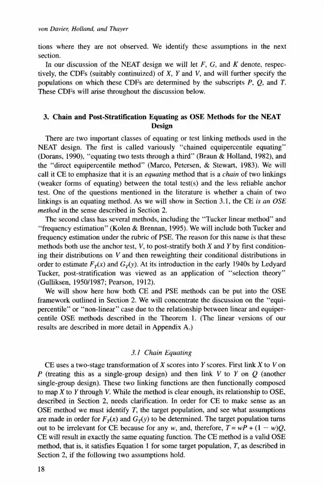
tions where they are not observed. We identify these assumptions in the next section.

In our discussion of the NEAT design we will let F, G, and K denote, respec- tively, the CDFs (suitably continuized) of X, Y and V, and will further specify the populations on which these CDFs are determined by the subscripts P , Q, and T. These CDFs will arise throughout the discussion below.

3. Chain and Post-Stratification Equating as OSE Methods for the NEAT Design

There are two important classes of equating or test linking methods used in the NEAT design. The first is called variously “chained equipercentile equating” (Dorans, 1990), “equating two tests through a third” (Braun & Holland, 1982), and the “direct equipercentile method” (Marco, Petersen, & Stewart, 1983). We will call it CE to emphasize that it is an equating method that is a chain of two linkings (weaker forms of equating) between the total test(s) and the less reliable anchor test. One of the questions mentioned in the literature is whether a chain of two linkings is an equating method. As we will show in Section 3.1, the CE is an 0% method in the sense described in Section 2.

The second class has several methods, including the “Tucker linear method” and “frequency estimation” (Kolen & Brennan, 1995). We will include both Tucker and frequency estimation under the rubric of PSE. The reason for this name is that these methods both use the anchor test, V, to post-stratify both X and Y by first condition- ing their distributions on V and then reweighting their conditional distributions in order to estimate FAX) and G,b). At its introduction in the early 1940s by Ledyard Tucker, post-stratification was viewed as an application of “selection theory” (Gulliksen, 1950/1987; Pearson, 1912).

We will show here how both CE and PSE methods can be put into the OSE framework outlined in Section 2. We will concentrate the discussion on the “equi- percentile” or “non-linear ” case due to the relationship between linear and equiper- centile OSE methods described in the Theorem 1. (The linear versions of our results are described in more detail in Appendix A.)

3. I Chain Equating

CE uses a two-stage transformation of X scores into Y scores. First link X to V on P (treating this as a single-group design) and then link V to Y on Q (another single-group design). These two linking functions are then functionally composed to map X to Y through V. While the method is clear enough, its relationship to OSE, described in Section 2, needs clarification. In order for CE to make sense as an OSE method we must identify T, the target population, and see what assumptions are made in order for FAX) and G.&) to be determined. The target population turns out to be irrelevant for CE because for any w, and, therefore, T = wP + (1 - w)Q, CE will result in exactly the same equating function. The CE method is a valid OSE method, that is, it satisfies Equation 1 for some target population, T, as described in Section 2, if the following two assumptions hold.

18

Chain and Post-StratiJicution Equating Methods

Assumption 1: Given any target population T of the form given in Equation 6, the link from X to V is population invariant, so that

Kp-'oFp(x) = KT-'0F&). (7) Assumption 1 makes use of the fact that KT 'OFAX) is the equipercentile function linking X to V on population T, for any T. From Equation 7 it immediately follows that the distribution of X on T, that is implicitly assumed by CE, is

Ff(L+) = KpKp-'0Fp(x). (8) Note that FT(&) is defined in terms of CDFq that can be estimated directly from the observed data.

Assumption 2: Given any target population T of the form given in Equation 6, the link from V to Y is population invariant, so that

G ~ - ' O K , ( ~ ) = G;'OKJV). (9)

(10)

Equation 10 defines GT(o(y) in terms of CDFs that can be estimated directly from the observed data. We use the subscript (0 to indicate that F,, and G,, are the CE fornis for F, and G,

If we now apply Equations 8 and 10 to the computation of the composed link from X to V to Y, we get

From Equation 9 it immediately follows that

G,o(y) = KpKQ- 'oG,(y) or GT(Lq ' = G& 'oKQ0KF ' (x).

PXY f&) = G ( C ; l"&(C)(4

The chain of four CDFs and their inverses on the right-hand side of Equation 11 is the usual definition of the CE function. Equation 11 shows that it is, indeed, an OSE function of the form given in Equation 1. This proves that CE is an OSE method.

We note that because the target population, T, cancels out in Equation 11, the function G, 'oK,oK~'oFI,(x) is the CE function for any T. As a consequence of Assumptions 1 and 2, the CE function is expected to be population invariant. However, in a real situation, Assumption 1 and/or Assumption 2 might not hold and there is no direct way to test that they do hold.

Note that the expected population invariance of the CE function is only strictly true for populations of the form given in Equation 6. To see this latter point, suppose that T is a subpopulation of P. In this circumstance, Assumption 2 is a bona fide assumption that could be either correct or incorrect, but is untestable because Y is never observed on I". However, Assumption 1 is directly testable because X is observed on P and, therefore, on T. Because of this, Assumption 1 can be directly refuted by the data and so it is not an assumption at all. Instead, Assumption 1 is an empirical relationship that is either correct or incorrect when T is a subpopulation of P .

19

von 1l)avieG Holland, und Thayer

3.2 Post-Stratification Equating

In PSE we estimate the distributions of both X and Y on a target population T of the form given in Equation 6 and then compute the equipercentile equating function as in Equation 1. Because T is mixture of P and Q we need to estimate the distribution of X in Q and the distribution of Y in P , where neither test is observed. PSE makes the assumption that the conditional distribution of X given V and the conditional distribution of Y given V are population invariant. In this discussion we let A x ) denote the score probabilities for X and k(v) the score probabilities for V , with subscripts to indicate which population these are for. We also let gcy) denote the score probabilities for Y in the same way. We state the assumptions for PSE formally, in a way that is parallel to Assumption 1 and Assumption 2, as follows.

Assumption 3: Given a target population T of the form given in Equation 6, the conditional distribution of X given V is population invariant, that is,

(12) f,4x I v) = f A x I v) =fQb I v) and, therefore,

Assumption 4: Given a target population T of the form given in Equation 6, the conditional distribution of Y given V is population invariant, that is,

K & b ) = K h l 4 = K P b l v ) (14)

Once the score probabilities, fT(Pc,(x) and g l (P( . , b ) , are computed by the post- stratification reweighting indicated in Equations 13 and IS, the corresponding CDFs, FT(ps,(x) and GTCPL9(y), are computed by continuking the discrete distribu- tions specified by fT(Pc,(x) and gIcPC,(y). Thus, F,(,, and GI(,,, are the solutions for F , and G T for PSE. X is equated to Yon T through

(16) eXY I(P5)(?c) = GT(PS)- ‘°FT(PS)(n).

Note that the equating function, exy ,(I,,)(x), cun depend on the choice of Tunlike exynCj(x) . Therefore, PSE can be different from CE, though they can also be identical in particular circumstance that we now discuss.

As a final comment to this section, we wish to point out that Theorem 1 is limited to appropriate comparisons between linear and equipercentile equating functions. In Appendix A we discuss the linear versions of both CE and PSE and Theorem 1 applies separately to each of these cases. It applies to a comparison of a CE equipercentile function to the chain linear function, and to a comparison of a PSE equipercentile function to the PSE linear function described in that appendix. It would not apply to comparing, for example, chain equipercentile to Tucker linear equating, or to a comparison of “frequency estimation” to chain linear equating.

20

Chain and Post-Stratification Equating Methods

4. Two Ideal Cases Where CE and PSE Both Give the Same Results

One of the important roles of the anchor test in NEAT design is to provide information about differences in the abilities of the examinees in the two popula- tions, P and Q. This is always limited by what Vmeasures and is why the anchor test should be appropriately constructed. Brennan and Kolen (1987) discuss condi- tions needed for an appropriate anchor test.

Marco, Petersen, and Stewart (1983); Petersen, Marco, and Stewart (1982); and Angoff and Cowell (1985) examined a number of equating methods, with or without an anchor test, varying the similarity of the examinee groups. Other studies focused on matching on the anchor for equating (Lawrence & Dorans, 1990; Livingston, Dorans, & Wright, 1995). These enipirical studies are summariLed well by Kolen’s observation:

finding is that, whcn the anchor test design is used to equate carefully constructed alternate forms, the groups taking the old and new forms are similar to one another, and the common set is a miniature version of the total test form, then equating methods all tend to give similar results. (Kolen, 1990, pp. 98-99)

Theorem 2, given next, is an analytical statement of a part of this empirical observation. More precisely, our first result concerns the case when the anchor test has the same distribution on both P and Q (without any additional assumptions about how similar X and Y are or about the anchor test being “a miniature version of the test”). In this situation we show that, as they are described in Section 3, both CE and PSE will result in exactly the same equating function.

Theorem 2: If, in the NEAT design, we have K p = KQ, then both CE and PSE yield the same equating function and it is

(17) Proof: The case for CE is obvious because the composition, KQoKF ‘(x) now equals the identity function, so that it cancels out, that is,

- I E X Y T ( O ( 4 = ~ X Y , ( f 3 , ( - 4 = G, or‘,(x>.

exy r(o(x) = G , ‘oKQoKF ‘OF&) = G& ‘OF&). (18) For the case of PSE, suppose Kr, = K,, then the score probabilities must also satisfy k,> = k , so that

k , = wkp + (1 - w)kg = k,, = k,, for any T = W P + (1 - w)Q.

Hence,

and

Once continuized, we must also have Fn,>,,(x) = Fr,(x), and G,,,(y) = GQ(y), from which the result for PSE follows.

21

von Davier, Holland, and Thayer

Theorem 2 shows that CE and PSE must yield nearly identical results when the two populations are very similar in the distribution of abilities measured by V.

Theorem 3 (below) addresses a case where the distribution V can be very different on P and Q, but where V is highly correlated with both X and Y. While the statement of Theorem 3 is probably stronger than necessary, we include it because results similar to it lie behind the often-stated view that a high correlation between the anchor and each operational test is important.

Theorem 3: If, in the NEAT design, we have X = V = Y, so that there is a perfect correlation between the anchor test and the other two tests, then both CE and PSE give the same equating function and it is the identity function:

(21) Proof: Because X = V = Y we have F,(x) = G,(x) = K7(x) for any T. The case for CE follows from the fact that now both G, '0KQ(x) = x and K,, 0FP(x) = x so that

(22)

RXY ,&) = exy 7(PS,(X> = x.

exy T(c,(x) = GQ- loKQ(K;loF,,(x)) = G, 'OK&) = x,

1

regardless of how different F,, and G, are.

For the case of PSE, note that the conditional score probabilities.f,(xl v),f,(xl v). g,(yI v) and gQ(y I v), are all 0 unles\ x = v = y , and then they equal 1. Then the score probabilities satisfy

and

or

Because the two sets of score probabilities are the same, oiice continuized, we must also have FIYPC,(x) = G7(PC,(x), from which the result for PSE follows.

Theorem 3 might seem obvious at first sight, but it shows that when the anchor test is perfectly correlated with the two other tests, then CE and PSE are both population invariant and identical (no matter how big the difference is between the two populations!).

Theorems 2 and 3 are simple but they show that we can distinguish between CE and PSE when the distribution of V on P is suflciently different from its distribution on Q, and when V is sufficiently different from X and Y. This is the case that we will implicitly assume in the rest of this article.

5. The Dorans and Holland RMSD Measure in the NEAT Design

Dorans and Holland (2000) define a measure of the degree to which an equating procedure fuils to be population invariant across a given set of subpopulations of a base population, In the applications of their methods to date they do not consider

22

Chuiri and Post-Strutz@ution Equuting Methods

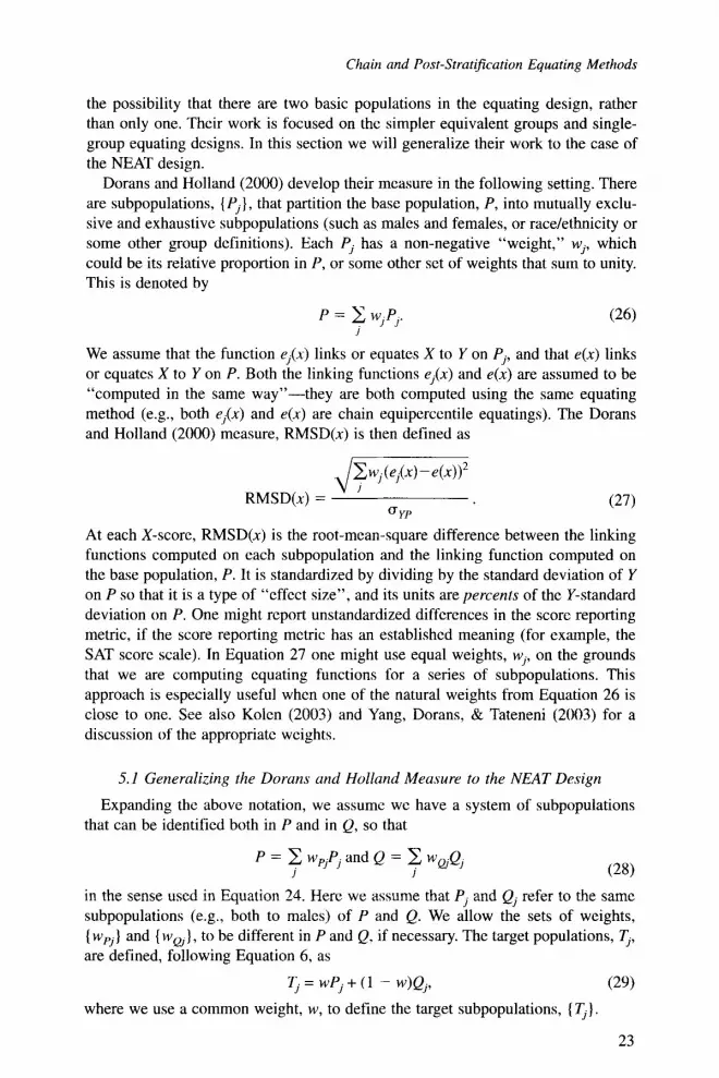
the possibility that there are two basic populations in the equating design, rather than only one. Their work is focused on the simpler equivalent groups and single- group equating designs. In this section we will generalize their work to the case of the NEAT design.

Dorans and Holland (2000) develop their measure in the following setting. There are subpopulations, {P,}, that partition the base population, P, into mutually exclu- sive and exhaustive subpopulations (such as males and females, or race/ethnicity or some other group definitions). Each P, has a non-negative “weight,” wl, which could be its relative proportion in P, or some other set of weights that sum to unity. This is denoted by

P = W;P,. i

We assume that the function e,(x) links or equates X to Yon P,, and that e(x) links or equates X to Yon P . Both the linking functions e,(x) and e(x) are assumed to be “computed in the same way”-they are both computed using the same equating method (e.g., both e,(x) and e(x) are chain equipercentile equatings). The Dorans and Holland (2000) measure, RMSD(x) is then defined as

(27)

At each X-score, RMSD(x) is the root-mean-square difference between the linking functions computed on each subpopulation and the linking function computed on the base population, P. It is standardized by dividing by the standard deviation of Y on P so that it is a type of “effect size”, and its units are percents of the Y-standard deviation on I-’. One might report unstandardized differences in the score reporting metric, if the score reporting metric has an established meaning (for example, the SAT score scale). In Equation 27 one might use equal weights, w,, on the grounds that we are computing equating functions for a series of subpopulations. This approach IS especially useful when one of the natural weights from Equation 26 is close to one. See also Kolen (2003) and Yang, Dorans, & Tateneni (2003) for a discussion of the appropriate weights.

5. I Genemlizing the Doruns und Holland Measure to the NEAT Design

Expanding the above notation, we assume we have a system of subpopulations that can be identified both in P and in Q, so that

P = C wPiPi and Q = waQJ i i in the sense used in Equation 24. Here we assume that PJ and Q, refer to the same subpopulations (e.g., both to males) of P and Q. We allow the sets of weights, [ kvpJ) and { w ~ ) , to be different in P and Q, if necessary. The target populations, T,, are defined, following Equation 6, as

(2% 7; = wP, + (1 - w)Q,, where we use a common weight, w, to define the target subpopulations, { T, ) .

23

von Daviel; Hollmd, and Thayer

In order to apply the results of Section 5, we simply restrict attention to each pair (P,, Q,) and use the data structure:

X V Y

Pi I/ I/ (30)

Qj I/ I/.

Then we compute the linking functions using the data from Pi and Qj. This results in the linking functions exy;Ti(cr)(x) for CE and exy;,j(ps)(x) for PSE. They are given by:

exy,n(c,(x) = ti, '0KmoK,,j 'oFry(x), (31)

(32)

and - 1 exy;7j.cps,(x) = G7ycr>s) o~TicE~.+).

We note that the CE function, is sensitive to j , but it is insensitive to the choice of weight, w, used to define the target mixture subpopulation, T,. In contrast, the PSE function, exy,Ticl,s,(x), can be sensitive both to the choice of w and to the subpopulation, T,.

In addition, let the CE and PSE equating functions for the whole target popula- tion, T, be denoted by eXy,,(&) and exy;T(pLs)(x).

We may now simply apply thc definition of RMSD(x) in Equation 27 to either CE or PSE with Pj replaced by und P replaced by T. The choice of the weights (w , } in Equation 27 is arbitrary and can be made in a variety of ways. If we have identified the various subpopulations, (P,} and (Q,}. because we are equally interested in all of them, then a case can be made that they should be given equal weight in the definition of RMSD(x). There are other possible choices that reflect the sizes of the (P,} and {Q,} (see, for example, Kolen, 2003; or Yang, Dorans, & Tateneni, 2003, for a discussion of the appropriate weights). However, the choice of the denominator, uyr, depends on which assumption we make, either CE or PSE. They need not agree. We consider these two cases next.

5.2 The Chain-Equating Cuse

In this case, we should use an estimate of ( J ~ that is compatible with the CE assumption that GT((?(y) = KpK&'oGe(y). This CDF does depend on T (because K , does) while the CE function, exy ,(&), does not. Hence, finding an estimate of ufl that is compatible with GTo)(y) could be a complicated problem. As an expedient, we suggest using ( J ~ ~ that is given (Al l ) in Appendix A for chain linear equating. It assumes more than we do here, but because it is simple to estimate, and is related to CE, it may be a reasonable choice. Hence, we propose the follouing definition of RMSD,,.(x):

with

24

Chain und Post-Stratifiration Equating Methods

M; = W(WPJ) + (1 - w)wa, (34) where wpJ and wa are given in Equation 28 and w is arbitrary, since CE does not depend on T. We might consider taking the same w as in Equations 6 or 29, for the PSE. Alternatively, we might use equal weights, wJ, on the grounds that we are computing equating functions for a series of subpopulations.

5.3 The Post-Strutificution Equating Cuse

Here the situation is different. There are “natural” weights given by Equation 34, where wPJ and w

The weights in Equation 34 may be useful because they reflect w in the definition of T. However, instead of using Equation 34, we might use equal weights, w,, on the grounds that we are computing equating functions for a series of subpopulations. For that reason we ought to give equal weight to them all, other- wise, why are we computing separate equating functions on them in the first place? See Kolen (2003) and Yang, Dorms, &L Tateneni (2003) for a discussion of the appropriate weights.

In order to get value for uTr for PSE in the NEAT design, we suggest using the value that is computed directly in the Linear PSE method described in Appendix A. An alternative is to use the value for the standard deviation of Y on T that is obtained by the Tucker linear method for the target population, T = wP + ( 1 - w)Q. This is given in Equation A18 (see Appendix A). These choices are similar to the one we propose for CE. Applying these ideas, the equation for RMSD(,,(x) is given by

are given in Equation 28 and w from Equation 6 or 29. ?

J E w J ( e X Y , T ( P c T ) ( x ) - e X Y , , ( p s ) ( X ) ) 2

(35) J

RMSD,ps,(x) = (7 TT

The two measures, RMSD,&) and RMSD,,(x), can be used to evaluate the sensitivity of CE and PSE to the subpopulations defined by { P ) ] and { Q } . We do not investigate these measures in more detail in this article. We introduce them here to show how the Dorans and Holland measure RMSD can be generalized to the NEAT design and that these generalizations will be slightly different for the CE and PSE methods. That two different measures are needed for the two methods makes their comparison somewhat problematic. We regard this as a useful topic for future research on population invariance measures.

Summary In this article we have shown that both CE and PSE are examples of OSE

methods using the precise definition given in Equation 1 . We give some ideal conditions when these two methods yield the same results. In addition, we define versions of the Dorans and Holland (2000) measures of population invariance of equating functions that can be applied to the NEAT design. The indices investigated and extended here add to the list of criteria that are overviewed by Harris and Crouse (1993).

While it is too early to say much about the two methods, CE and PSE, using our approach, with more examples we may be able to quantify their relative sensitivity

25

von Daviec Holland, und Thaycr

to the equating population in various situations of interest. We expect that two factors will be important in studies using our approach. First, the correlations of the anchor test with the operational tests. Second, how different the subpopulations are on the anchor test scores. These factors are known to play a role in the NEAT design and our methods provide another way to examine their effects (see Dorans, Holland, Thayer, & Tateneni, 2003, for the application of the methods outlined here).

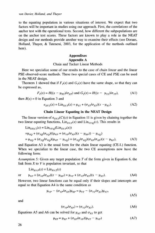
Appendixes Appendix A

Chain and Tucker Linear Methods

Here we specialize some of our results to the case of chain linear and the linear PSE observed-score methods. These two special cases of CE and I'SE can be used in the NEAT design.

Theorem 1 showed that if FAX) and G,(x) have the same shape, so that they can be expressed as,

('41)

(A21

F A X ) = H((x - ~ ~ ~ ) / ( r ~ ~ ) and G,O) = H((x - P ~ J U ~ ) , then R(x) = 0 in Equation 3 and

ex,,G) = IdinXKA-4 = P>7 + (UdGXTXX -Pxr).

Chain Linear Equating in the NEAT Design

The linear version of eXr,,(C)(x) in Equation 11 is given by chaining together the two linear equating functions, Lin,,.,,(x) and lin,KL?(v). This results in

Lin,,&) = Lin,,Q(LinxKP(4)

=PYQ + (UU~~V&(PW + ((rv,JffxP>(x - CLXP)) - P"Q)

= PYQ + (UY&J"Q)(PVP - PVQ) + (aY~JavQ)(Uvd(JxP~(x - P X f A ( A 3 and Equation A3 is the usual form for the chain linear equating (CE-Id) function. When we specialize to the linear case, the two CE assumptions now have the following form:

Assumption 5: Given any target population T of the form given in Equation 6, the link from X to V is population invariant, so that

Lin,,, (x) = Linx,.x) Or PW + ((JVr/uXf)(x - PXP) = PVr + ('V7/uXT)(x - PXT). ('44) However, two linear functions can be equal only if their slopes and intercepts are equal so that Equation A4 is the same condition as

PVP - ((TdJXP)PXP = Pv7 - (o,,/(rxT)Pxn 045)

(Crvp/Uxp> = (Uv7/(Jxr). (-46)

('47)

and

Equations A5 and A6 can be solved for pxT and a,,. to get

PXT = PXP + ('XfJUVf)(PV7' - P V f )

26

and

ax , = (uv7/uVP)flXp. (A8) Assumption 6: Given any target population T of the form (Equation 6), the link from X to V is population invariant, so that

L i n , Q ( v > = Linvy.Av) Or PYQ + ((JYd(rVQ)(v - PVQ) = k"+ (ay7/(TW)(v - PW). 649) A similar argument to the one for Assumption 5 shows that Equation A9 is equivalent to

(A 10)

u Y l = ('VI/aVQ)(rYQ. (All)

PYT = PYQ + (aY,Ja"Q)(PvT - PVQ) and

Applying Equations A7, A8, AIO, and A l l to the CE-L function (Equation A3), and simplifying the expressions results in

Li"XY(C.)(4 = PYT + ( U d ( J X T ) ( X - PX,). (A 12) This shows that LinxY(c)(x) defined in Equation A3 is, in fact, Linxy,Ax) as

defined in Equation A2. The target population, T, cancels out of the composed function (Equation A3). This provides a direct argument that chain linear equating is linear OSE on T with pxT, a,, pxT, and ox,. given by the expressions in Equations A7, A8, A 10, and A 1 1. Note that an in Equation A1 1 can be used in the RMSD formula for CE (Equation 33).

'bcker Linear Equating in the NEAT Design There are several good discussions of the Tucker linear OSE method (e.g.,

Angoff, 1971/1984; Gulliksen, 1950/1987; Kolen & Brennan, 1995). We will just point out the parallels to the PSE assumptions given in Section 3. Instead of the conditional probability functions that we use in Assumptions 3 and 4, the assump- tions of the Tucker method can be stated in terms of conditional means and variances.

Assumption 7: Given any target population T of the form given in Equation 6, the conditional mean and standard deviation of X given V are population invariant and, furthermore,

E(X1 V , 7J = E(XI V, P ) = up + hpV (A1 3) (i.e., lineur regression) and

SD(Xl v, 7J = SD(X) v, P ) = u p ,

(i.e., consfuant residual variance).

Assumption 8: Given any target population T of the form given in Equation 6, the conditional mean and standard deviation of Y given V are population invariant and, furthermore,

E( Y 1 v, T) = E( YI v, Q ) = UQ + bQv (A15) and

27

von Daviel; Holland, and Thayer

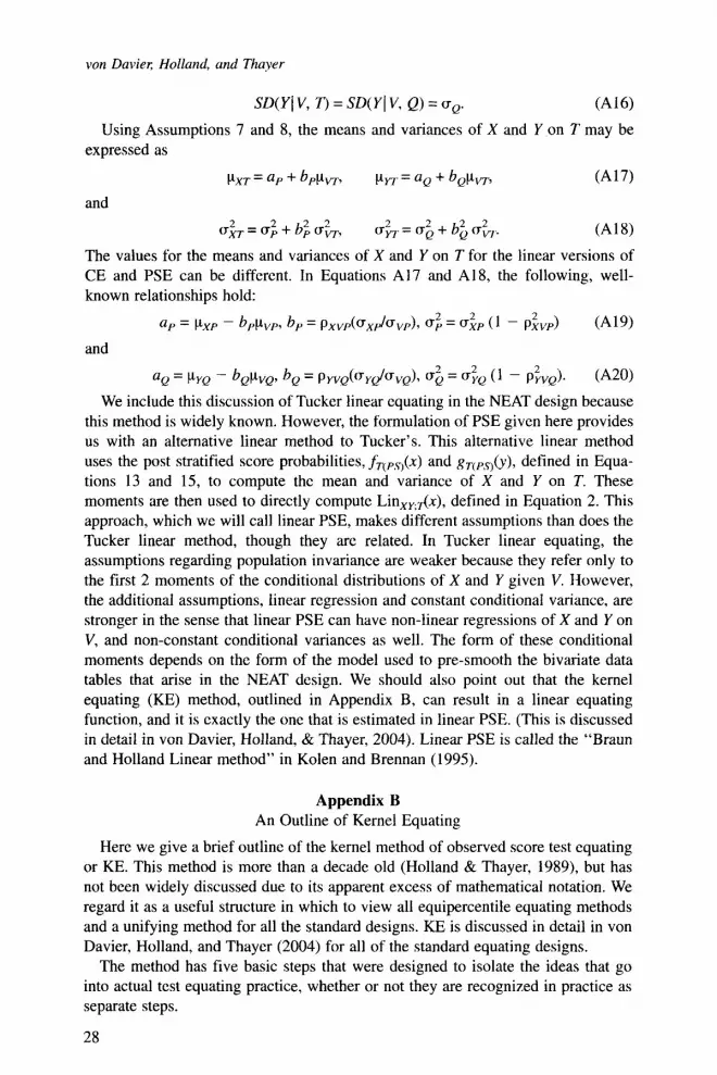
sD(YI v, = sD( YI v, Q ) = UQ. (A 16) Using Assumptions 7 and 8, the means and variances of X and Y on T may be

expressed as

PXT = + h P p v T , c(YT = uQ + bQPVT, (A17) and

uiT = u; + b: u&.. u’, = D; + b; u$,.

The values for the means and variances of X and Y on T for the linear versions of CE and PSE can be different. In Equations A17 and A18, the following, well- known relationships hold:

2 2 2 U P = P X P - b,CL,T9 h P = Px, (~xFJ~,w)9 u p = U X P (1 - PXVP)

= PYQ - b,~vQ> hQ = P Y V Q ( ( T Y ~ U V Q ) , u~ = urc, (1 - PYVQ).

(A19)

(A20)

and 7 2 2

We include this discussion of Tucker linear equating in the NEAT design because this method is widely known. However, the formulation of PSE given here provides us with an alternative linear method to Tucker’s. This alternative linear method uses the post stratified score probabilities, fT(Ps)(x) and gT(pLyl(y), defined in Equa- tions 13 and 15, to compute the mean and variance of X and Y on T. These moments are then used to directly compute Lin,,,{x), defined in Equation 2. This approach, which we will call linear PSE, makes different assumptions than does the Tucker linear method, though they are related. In Tucker linear equating, the assumptions regarding population invariance are weaker because they refer only to the first 2 moments of the conditional distributions of X and Y given V. However, the additional assumptions, linear regression and constant conditionaI variance, are stronger in the sense that linear PSE can have non-linear regressions of X and Yon V, and non-constant Conditional variances as well. The form of these conditional moments depends on the form of the model used to pre-smooth the bivariate data tables that arise in the NEAT design. We should also point out that the kernel equating (KE) method, outlined in Appendix B, can result in a linear equating function, and it is exactly the one that is estimated in linear PSE. (This is discussed in detail in von Davier, Holland, & Thayer, 2004). Linear PSE is called the “Braun and Holland Linear method” in Kolen and Brennan (1995).

Appendix B An Outline of Kernel Equating

Here we give a brief outline of the kernel method of observed score test equating or KE. This method is more than a decade old (Holland & Thayer. 1989), but has not been widely discussed due to its apparent excess of mathematical notation. We regard it as a useful structure in which to view all equipercentile equating methods and a unifying method for all the standard designs. KE is discussed in detail in von Davier, Holland. and Thayer (2004) for all of the standard equating designs.

The method has five basic steps that were designed to isolate the ideas that go into actual test equating practice, whether or not they are recognized in practice as separate steps.

28

Chuiri and Post-Strutificution Equating Methods

Step 1: Pre-smoothing. In this step, the data that are collected in an equating design are “pre-smoothed” using standard statistical procedures designed to esti- mate the actual score distributions that arise in the equating design. Pre-smoothing, using various techniques, has become a standard tool in various approaches to equipercentile equating.

We advocate using log-linear models for univariate and bivariate score distribu- tions, as discussed in Holland and Thayer (2000), because of their extreme flexibil- ity and ability to accommodate the many unusual features of score distributions that arise in practice. The results of this pre-smoothing process are twofold. First, the smoothed score distributions that are needed for the rest of the equating process are obtained, and second, a matrix that can be used to calculate the standard error of equating later on in the process is computed. Every pre-smoothing method has such a matrix, but the log-linear methods have a standard way of finding it in an efficicnt manner. This is discussed in detail in Holland and Thayer (2000).

Step 2: Estimating score distributions for the target population. Once the pre-smoothing has been done, there are formulas, depending on the equating design, that use the smoothed score distribution estimates to produce estimates of the score probability distributions on T, which we call r and s, where

r, = P { X = xJ I T } , sk = P { Y = yk 1 T )

r = (r,, . . . , rJ) and s = (st, . . . , sK).

(BI)

(B2) es for X are associated with the X-raw scores, (x , } , and those

for Yare associated with the Y-raw scores, ( y k } . Depending on the equating design the formulas for r and s range from the simple identity function to the complexities implicit in anchor test methods.

Step 3: Continuizing the discrete score distributions. This step is often over- looked in discussions of equipercentile equating methods, but it occurs in all of them. We start with discrete score distributions for X and Yon T and turn these into continuous score distributions over the whole real line. It is similar to approximat- ing the probabilities from the dim-ete binomial distribution by probabilities from the continuous normal distribution. Thus, it is a step that looks like an everyday statistical method, but it is actually unusual because the entire discrete distribution is changed into a continuous one that is “close” to the original in a sense that is often left vague. Our approach is to make this step explicit and to make the sense of the approximation clear. Older equipercentile equating methods replace the discrete score distributions by piece-wise linear CDFs based on “percentile ranks.” The (Gaussian) kernel method of continuizing r uses the formula

and the vectors r and s are given by

where,

29

von Duviel; Holland, and Thuyer

@(z) denotes the standard N(0, 1) CDF, x ranges over (-m,+=), and h, > 0. FAX; h,) is the continuized CDF based on the discrete score distribution determined by r and (x,). pxT and crZxT, given above, are the moments of X on T that can be used in linear PSE mentioned in Appendix A.

The continuized G&, h,) is computed in a similar way using the score probabili- ties from s, and the Y-scores, ( y L } .

An essential feature of Gaussian kernel continuization is the choice of the “bandwidths,” h, and h,. We recommend using a penalty function to select the bandwidths automatically to make the density functions, f A x ; h,) and g&-y, h,), derived from FAX; h,) and G,e , h,) both smooth and able to track the essential features of the smoothed discrete score probabilities. We have found the following penalty functions to give good results.

PENALTY ,(h) = [ (r , /4) - fr(xj; h)]*, j

where, dJ is the “width” of the interval associated with the score xJ (often these widths are all set equal to 1).

(B5) PENALTY,(h) L- 2 AJ(l - BJ), J

where A, = 1 if the derivative off&; h) with respect to x, u(x; h), is less than 0 a little to the left of xJ, and B, = 0 if u(x; h) > 0 a little to the right of xJ. Thus, we get a penalty of 1 for every score point where the densityf,(x; h) is “U-shaped” around it. What “near” means is a parameter of PENALTY,(h) and we can combine the two penalties with a weight, that is

PENALTY,(h) + K*PENALTY,(h). (B6) We have found K = 1 to be useful in several applications where there are teeth or gaps in the distribution that need to be smoothed out. Standard derivative-free methods can be used to minimize these penalty functions in order to choose h. Separate continuizations of the two discrete score distributions are carried out, resulting in FAX; h,) and G&; hy) .

Step 4: Computing the equating function. Once all the above work is done, the KE equipercentite equating function can be computed directly as the function composition:

(R7) ex+) = G , ’(F,(x; h,); hy), where G,’(p; hy) denotes the inverse of p = G&; hy) .

Step 5: Computing the standard error of equating. The standard error of equating (SEE) for ex&) depends on three factors that correspond to the above four steps-pre-smoothing, computing r and s from the smoothed data, and the combination of continuization and the mathematical form of the equating function from step 4. Being based on analytical formulas, KE allows us to use the Taylor expansion or “delta method” to compute the SEE for a variety of equating designs. The main difference between the various equating designs, as far as computing the SEE for KE is concerned, is Step 2. Each design requires a different formula for

30

Chain and Post-Stratification Equating Methods

mapping the pre-smoothed data to the score probabilities, r and s, but the contribu- tions of the other steps to the SEE are the same for all designs. This observation allows a general computing formula for the SEE to be devised for KE that reflects pre-smoothing, the equating design, and the use of Gaussian kernel smoothing for continuizing the discrete CDFs.

Note We would like to thank Skip Livingston and Henry Braun, and two anonynious reviewers

for their comments on earlier drafts of this article. In addition, we have received helpful comments and suggestions from our colleagues Neil Dorans, Krishna Tateneni, and Wen- Ling Yang during the development of this project. The ETS Research Allocation supported our work. This research is ColkIbOrdtiVe in every respect and the order of authorship is alphabetical.

References

Angoff, W. H. (1971). Scales, norms, and equivalent scores. In R. 1,. Thomdike (Ed.), Educational meusurenzent (2nd ed., pp. 508400). Washington, DC: American Council on Educational. (Reprinted from Scales, norms, and equivalent scores, by W. H. Angoff, 1984, Princeton, NJ: Educational Testing Service.)

Angoff, W. H., & Cowell, W. R. (1985). An examination of the assumption that the equating of parallel forms is population-independent (ETS Research Report 85-22). Princeton, NJ: Educational Testing Service.

Braun, H. I., & Holland, P. W. (1982). Observed-score test equating: A mathematical analysis of some ETS equating procedures. In P. W. Holland & D. B. Rubin (Eds.), Test equating (pp. 4-49). New York Academic Press.

Brennan, R. L., & Kolen , M. J. (1987). Some practical issues in equating. Applied Psycho- logical Measurement, 11, 279-290.

von Davier, A. A,. Holland, P. W., & Thayer, D. T (2004). The kernel method of test equating. New York: Springer Verlag.

Dorans, N. J. (1990). Equating methods and sampling designs. Applied Measurement in Education, 3, 3-17.

Dorans, N. J., & Holland, P. W. (2000). Population invariance and the equatability of tests: basic theory and the linear case. Journal of Educational Measurement, .37, 281-306.

Dorans, N. J., Holland, P. W., Thayer, D., & Tateneni, K. (2003). Invariance of score linking across gender groups for three advanced placement program examinations. In N. J. Dorans (Ed.), Population invuriurice of score linking: Theory and applications to Advanced Placement Program examinations (ETS RR-03-27, pp. 79-1 18). Princeton, NJ: Educa- tional Testing Service.

Gulliksen, H. (1950). The theoiy ofmental tests. New York: Wiley. (Reprinted in 1987 by Lawence Erlbaum Associates: Hillsdale, NJ).

Harris D. J., & Crouse, J. D. (1993). A study of criteria used in equating. Applied Measure- ment in Education, 6, 195-240.

Holland, P. W., & Thayer, D. T. (1989). The kernel method of equating score distributions (Research Report 89-7). Princeton, NJ: Educational Testing Service.

Holland, P. W., & Thayer, D. T. (2000). Univariate and bivariate loglinear models for discrete test score distributions. Journal of Educational and Behavioral Statistics. 25, 133-1 83.

31

von Davies Holland, and Thuyer

Kolen, M. J. (1990). Does matching in equating work? A discussion. Applied Meusurement in Education, 3(1), 97-104.

Kolen, M. J. (2003). Evaluating population invariance: A discussion of "population invar- ance of score linking: Theory and applications to advanced placement examinations". In N. J. Dorans (Ed.), Population invariance of score linking: Theory and applications to Advanced Placement Program examinations (ETS RR-03-27, pp. 1 19-1 25). Princeton, NJ: Educational Testing Service.

Kolen, M. J. , & Brennan, R. J. (1995). Test equating: Methods and pruc Springer.

Lawrence, I. M., & Dorans, N. J . (1990). Effect on equating results of matching samples on an anchor test. Applied Measurement in Education, 3( I), 19-36,

Livingston, S. A,, Dorans, N. J., & Wright, N. K. (1995). What combination of sampling and equating methods works best? Applied Measurement in Education, 3( I ) , 73-95.

Marco, G. L., Petersen, N. S., & Stewart, E. E. (1983). A test of adequacy of curvilinear score equating models. In Weiss, D. J. (Ed.), New horizons in testing (pp. 147-177). New York: Academic.

Pearson, K. (1912). On the general theory of the influence of selection on correlation and variation. Biometrika, 8, 437443.

Petersen, N. S., Marco, G . L., & Stewart, E. E. (1982). A test of adequacy of linear score equating models. In P. W. Holland and D. B. Rubin (Eds.), Test equating (pp. 71-135). New York: Academic.

Yang, W. L., Dorans, N. J. , & Tateneni, K. (2003). Effect of sample selection on AP multiple-choice score to composite score linking. In N. J. Dorans (Ed.), Population invariance of score linking: Theory and applications to Advanced Placement Program examinations. (ETS RR-03-27, pp. 57-78). Princeton, NJ: Educational Testing Service.

Authors ALINA A. VON DAVIER is a Research Scientist in the Center for Statistical Theory and

Practice, at Educational Testing Service, Rosedale Rd. MS 12-T, Princeton, NJ, 08541; avondavier@ets.org. Her research interests include traditional and IRT test equating and linking, multivariate analysis, causal inferences in non-experimental designs.

PAUL W. HOLLAND holds the Frederic M. Lord Chair in Measurement and Statistics at Educational Testing Service, Rosedale Rd. MS 12-T, Princeton, NJ, 08541; pholland@ets.org. He has made major contributions to the following areas: Statistical models for social networks, the analysis of multivariate categorical data, causal inference in experimental and non-experimental research, the foundations and computations of Item Response Theory, test equating, and Differential Item Functioning/"item bias."

DOROTHY T. THAYER is a consultant in the Center for Statistical Theory and Practice, at Educational Testing Service, Rosedale Rd. MS 12-T, Princeton, NJ, 08541 ; dthayer@ets.org. Her research interests include computational and statistical methodol- ogy, empirical Bayes techniques, missing data procedures and exploratory data analysis techniques.

32