Longitudinal patient stratification of electronic health records

Proceedings of Machine Learning Research 158:220–235, 2021 Machine Learning for Health (ML4H) 2021

Longitudinal patient stratification of electronic health recordswith flexible adjustment for clinical outcomes

Oliver Carr∗ [email protected]

Avelino Javer∗ [email protected]

Patrick Rockenschaub∗ [email protected]

Owen Parsons [email protected]

Robert Durichen [email protected]

Sensyne Health Plc, Oxford, UK

AbstractThe increase in availability of longitudinal elec-tronic health record (EHR) data is leading toimproved understanding of diseases and dis-covery of novel phenotypes. The majority ofclustering algorithms focus only on patient tra-jectories, yet patients with similar trajectoriesmay have different outcomes. Finding sub-groups of patients with different trajectoriesand outcomes can guide future drug develop-ment and improve recruitment to clinical trials.We develop a recurrent neural network autoen-coder to cluster EHR data using reconstruc-tion, outcome, and clustering losses which canbe weighted to find different types of patientclusters. We show our model is able to discoverknown clusters from both data biases and out-come differences, outperforming baseline mod-els. We demonstrate the model performance on29, 229 diabetes patients, showing it finds clus-ters of patients with both different trajectoriesand different outcomes which can be utilized toaid clinical decision making.

Keywords: Patient Stratification, Recur-rent Neural Network, Autoencoder, ElectronicHealth Records, Clustering

1. Introduction

Chronic diseases like diabetes or heart failure mayprogress very differently across patients (Spratt et al.,2017; Lewis et al., 2017) but the reasons for differen-tial progression are not yet well understood. Betweenpatient differences have been linked — among otherfactors — to the underlying pathology or to differen-tial response to treatment (Sarrıa-Santamera et al.,2020; Hedman et al., 2020).

∗ These authors contributed equally

Over the last decade, the spread of EHRs has en-abled the collection of unprecedented longitudinal pa-tient information (Shickel et al., 2018). Early workusing this rich data to investigate heterogeneous dis-ease progression mostly employed unsupervised clus-tering to find patient subgroups in the data that sharea similar medical history (Miotto et al., 2016; Bay-tas et al., 2017; Madiraju et al., 2018; Landi et al.,2020). However, EHR data are primarily designedfor clinical care and are not usually collected withresearch in mind. Identified clusters may thereforebe driven by spurious associations such as patientdrop out, selective recording, modifications of the ITinfrastructure, or administrative differences betweenhealthcare providers (de Jong et al., 2019; Ehrensteinet al., 2019).

In an attempt to address these issues, new methodshave been developed that focus on relevant patientoutcomes to guide the clustering of patient trajec-tories (Zhang et al., 2019; Lee and van der Schaar,2020; Lee et al., 2020), e.g., by including occurrenceof complications or time to death. In this so-calledpredictive clustering, a low-dimensional latent repre-sentation of the data is created that retains only infor-mation predictive of future clinical events. Patientsare grouped according to their similarity in this la-tent space. While this approach ensures clusters thatdiffer in the risk of experiencing the outcome, theyare unable to distinguish between distinct trajecto-ries that lead to similar risks.

Retaining trajectories, however, can be paramountto clinical interpretation. For example, although pa-tients with acute heart failure may have short-termmortality risks that are very similar to patients hos-pitalised with sepsis, the mechanisms that cause thehigh risk are quite different and a model should be

© 2021 O. Carr, A. Javer, P. Rockenschaub, O. Parsons & R. Durichen.

Longitudinal patient stratification with clinical outcomes

able to distinguish between them. In this work, wetherefore propose a novel semi-supervised architec-ture that combines both approaches — predictive andunsupervised — to guide clustering towards outcomesof interest while enforcing similarity on the inputscale. By doing so, we ensure that patients with verydifferent trajectories are not lumped into a commoncluster but remain in separate groups that facilitateclinical interpretation. Changing the weights of theunsupervised and predictive optimisation functions,the algorithm can be adjusted to prioritise one or theother. We refer to this approach as longitudinal pa-tient stratification by clinical outcomes (LPS-CO).We apply our method to right-censored clinical

data — which is ubiquitous in EHR data — and showhow it can lead to novel insights. Our main contri-butions can be summarised as follows:

• Introduction of a flexible semi-supervised patientstratification approach which identifies clustersof patients which share a similar medical historyas well as clinical outcomes through parallel op-timisation of an unsupervised and predictive lossfunction.

• Introduction of a Cox proportional hazards lossfunction to consider right-censored outcomes aspredictive targets such as time to death or re-hospitalisation.

We validate our proposed method on a syntheticdataset with known clusters as well as on a diabetescohort extracted from a longitudinal EHR datasetconsisting of approximately half a million patients.Comparisons to other baseline methods indicate howour approach can balance between unsupervised andpredictive clustering and discover novel patient clus-ters.

2. Related Work

Initial work in patient phenotyping mostly appliedclustering to cross-sectional data. Patient phenotyp-ing using k-means has been used early for examplein diabetes (Hammer et al., 2003) and heart fail-ure (Ather et al., 2009). Other commonly appliedmethods include hierarchical clustering (Moore et al.,2010; Burgel et al., 2010) and self-organising maps(Ather et al., 2009). Recently, these have been par-tially superseded by methods based on autoencoders,which provide an elegant way to deal with increas-ingly high-dimensional medical data. Notably, Xie

et al. (2016) proposed a deep embedded clustering(DEC) algorithm that uses an autoencoder with aself-supervised loss function to jointly learn the low-dimensional representation and cluster assignments.This approach has been used in Carr et al. (2020)and Castela Forte et al. (2021), among others, andprovides the basis for our proposed approach.

With the advent of EHRs and increasing availabil-ity of longitudinal patient data, unsupervised meth-ods have also been used for phenotyping of sequentialmedical data. Proposed models include generalisa-tions of classical methods (see for example Mullinet al. (2021)) as well as deep learning-based algo-rithms to longitudinal data. In the latter case, re-current autoencoders (Zhang et al., 2018; de Jonget al., 2019) or convolutions (Zhu et al., 2016) havebeen used to embed the time series.

When evaluating the groups identified during clus-tering via the above methods, patients are often com-pared based on the risk of experiencing clinically rel-evant outcomes. For example, Castela Forte et al.(2021) show that among intensive care patients, clus-ter membership was associated with risk of death.The analysis is entirely post-hoc, however, and differ-ences in risk did not directly influence the earlier clus-ter assignments. Recent works have aimed to incor-porate information of outcomes into the discovery ofclusters. Zhang et al. (2019) used a recurrent neuralnetwork (RNN) to predict markers of progression inParkinson’s disease and then employed dynamic timewarping (Berndt and Clifford, 1994) and t-distributedStochastic Neighbor Embedding (t-SNE) (van derMaaten and Hinton, 2008) to cluster patients basedon the hidden states of the RNN. Lee and van derSchaar (2020) proposed an actor-critic approach fortemporal predictive clustering (AC-TPC) in whichan RNN-based encoder/predictor network is trainedjointly with the cluster embeddings. This was ex-tended in Lee et al. (2020) to incorporate time-to-event outcomes via a novel loss function based on aWeibull-shaped parametric hazard.

In our work, we have adapted a RNN autoencoderthrough the addition of a clustering loss (Xie et al.,2016) and an outcome loss (Bello et al., 2019) andpropose flexible balancing of these losses, thereby al-lowing researchers to control the degree to which clin-ical outcomes should drive the clustering. This dif-fers from Zhang et al. (2019); Lee and van der Schaar(2020); Lee et al. (2020) who focus on outcomes with-out retaining trajectory information in the clusters.

221


3. Methods

This section describes the methods and models usedto obtain patient representations from patient trajec-tories and the clustering methods applied.Let D = {X ,Y}Nn=1 define the patient data, where

X is a set of covariate vectors, Y is a set of clini-cal outcomes, and N is the total number of patientsincluded in the data. D may describe each patientn’s observations at a single point of time {xn, yn} orlongitudinally over a period of time {xn

t , ynt }T

n

t=1. Sim-ilarly, Y may contain continuous outcomes yn ∈ R,binary outcomes yn ∈ {0, 1}, or time-to-event out-comes yn = {sn, cn} with sn ∈ R+ being the patient’sfollow-up time and cn ∈ {0, 1} being an indicator ofwhether the patient experienced the outcome of in-terest (1) or was censored (0). Going forward andwithout loss of generality, we omit the time subscriptt for simplicity and assume time-to-event data.Following Xie et al. (2016), we aim to cluster X into

K clusters, each of which is represented by a centroidvector λk for k = 1, ...,K. In order to deal with thechallenges posed by high dimensionality frequentlyobserved in EHR data, clustering is not performedin the input space but in a latent embedding spacecreated by a learned, non-linear function fθ : X → Z.

We combined three losses with correspondingweights to give the overall loss function,

L = wrLr + wyLy + wcLc, (1)

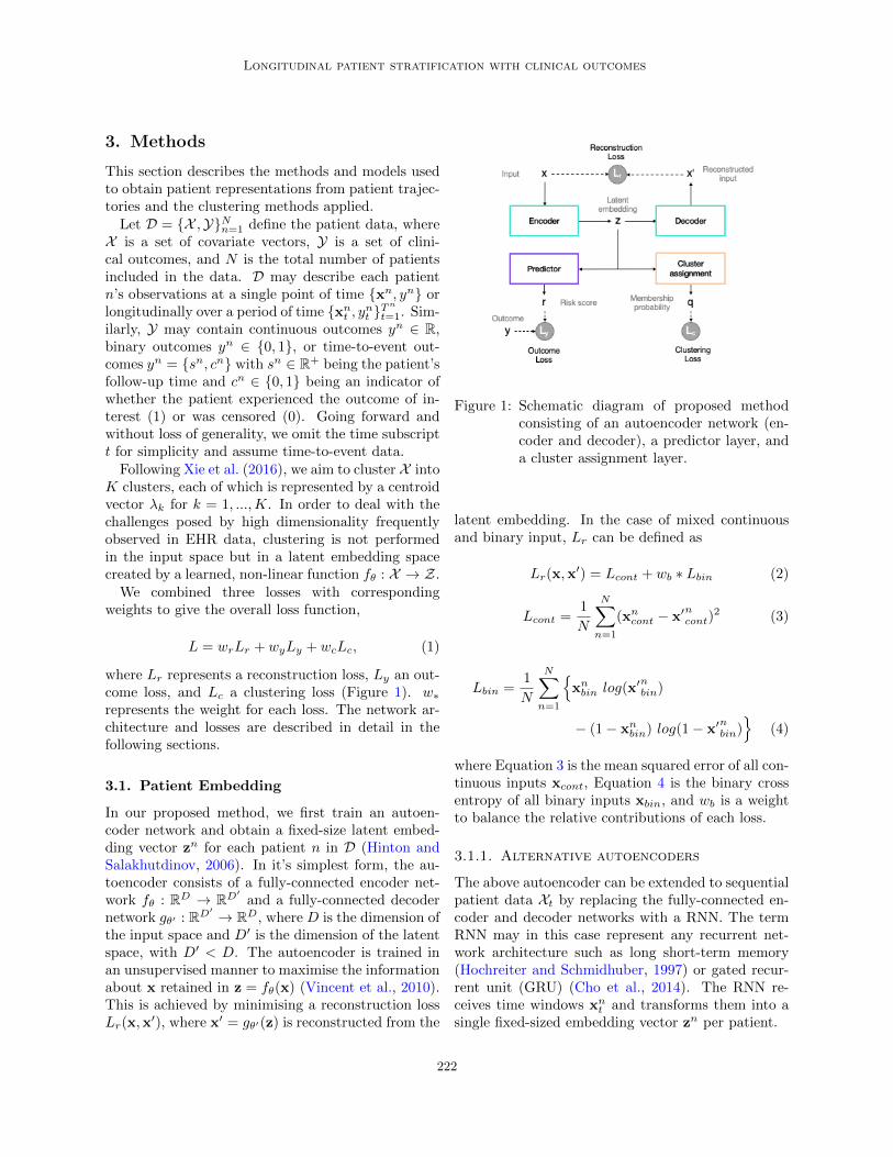
where Lr represents a reconstruction loss, Ly an out-come loss, and Lc a clustering loss (Figure 1). w∗represents the weight for each loss. The network ar-chitecture and losses are described in detail in thefollowing sections.

3.1. Patient Embedding

In our proposed method, we first train an autoen-coder network and obtain a fixed-size latent embed-ding vector zn for each patient n in D (Hinton andSalakhutdinov, 2006). In it’s simplest form, the au-toencoder consists of a fully-connected encoder net-work fθ : RD → RD′

and a fully-connected decodernetwork gθ′ : RD′ → RD, where D is the dimension ofthe input space and D′ is the dimension of the latentspace, with D′ < D. The autoencoder is trained inan unsupervised manner to maximise the informationabout x retained in z = fθ(x) (Vincent et al., 2010).This is achieved by minimising a reconstruction lossLr(x,x

′), where x′ = gθ′(z) is reconstructed from the

Figure 1: Schematic diagram of proposed methodconsisting of an autoencoder network (en-coder and decoder), a predictor layer, anda cluster assignment layer.

latent embedding. In the case of mixed continuousand binary input, Lr can be defined as

Lr(x,x′) = Lcont + wb ∗ Lbin (2)

Lcont =1

N

N∑n=1

(xncont − x′n

cont)2 (3)

Lbin =1

N

N∑n=1

{xnbin log(x′n

bin)

− (1− xnbin) log(1− x′n

bin)}

(4)

where Equation 3 is the mean squared error of all con-tinuous inputs xcont, Equation 4 is the binary crossentropy of all binary inputs xbin, and wb is a weightto balance the relative contributions of each loss.

3.1.1. Alternative autoencoders

The above autoencoder can be extended to sequentialpatient data Xt by replacing the fully-connected en-coder and decoder networks with a RNN. The termRNN may in this case represent any recurrent net-work architecture such as long short-term memory(Hochreiter and Schmidhuber, 1997) or gated recur-rent unit (GRU) (Cho et al., 2014). The RNN re-ceives time windows xn

t and transforms them into asingle fixed-sized embedding vector zn per patient.

222


Additionally, the simple autoencoder describedearlier may be replaced by any number of alternativearchitectures. For example, we found it beneficialin our experiments to use a variational autoencoder(VAE) instead (Kingma and Welling, 2014). In thiscase, the network learns a probabilistic rather thandeterministic patient embedding (commonly param-eterised as the means µ and variances σ2 of a D′

dimensional multivariate Gaussian distribution withdiagonal covariance structure) which in our experi-ments lead to a smoother, more continuous embed-ding space. Using a VAE and changes Lr to

Lr = − 1

N

N∑n=1

log pθ(xn|zn) (5)

− 1

2

D′∑d′=1

(1 + log(σ2d′)− µ2

d′ − σ2d′)

Equation 2 may be seen as a special weighted case oflog pθ(x|z) where all input dimensions are modelledas independently Gaussian (with fixed unit variance)or Bernoulli.

3.1.2. Pre-training of the autoencoder

As cohorts of interest often consist of much smallernumbers of patients than the total available (e.g.,only patients with incident of diabetes), a pre-training step is applied to learn patient embeddingsfrom all available data. This aims to learn a bet-ter representation between the wide range of diag-noses, procedures, medications, and laboratory mea-surements through time before updating the learnedpatient embeddings on just the cohort of interest.

3.2. Patient Outcomes

During pre-training, the autoencoder learns a lower-dimensional representation zn in an unsupervisedmanner. We propose to include a shallow fully-connected layer hϕ that relates zn to the risk of ex-periencing the outcome yn, estimating a scalar riskscore rn = hϕ(z

n).

The outcome is then included during training viathe additional loss function Ly. Depending on thenature of the prediction task, Ly may be chosen asthe mean squared error (regression) or binary cross-entropy (classification). For the case of right-censoredtime-to-event outcomes, we propose to use a loss

based on the partial likelihood of the Cox propor-tional hazards model (Bello et al., 2019), which isdefined as

Ly = − 1

N

N∑n=1

cn

rn − log∑

j∈R(sn)

exp(rj)

(6)

where c describes whether an outcome was observedfor the patient (cn = 1) or if the patient was cen-sored (cn = 0) and R(sn) represents the set of pa-tients still at risk after time sn, i.e., R(sn) = {i | i ∈{1, ..., N}, si ≥ sn}.

3.3. Patient Clustering

Once a patient embedding has been learned (with orwithout considering the outcome), standard cluster-ing methods may be applied (see for example Zhanget al. (2019)). Alternatively, cluster assignments maybe learned simultaneously with the patient embed-dings, which allows them to influence the learned em-beddings via back propagation and optimise them forclustering. Following Xie et al. (2016), we introducea clustering layer that learns the position of K clus-ter centroids λk ∈ RD′

. The probability qnk of patientembedding zn belonging to cluster k can then be cal-culated via an appropriate kernel, e.g., the density ofa Student’s t distribution:

qnk =(1 + ||zn − λk||2)−

12∑

k′(1 + ||zn − λk′ ||2)− 12

(7)

Cluster assignments are then iteratively refined Xieet al. (2016). Since true cluster labels are unknown,we instead use self-training via an auxilliary targetdistribution pnk that emphasise each patient’s highconfidence clusters

pnk =(qnk )

2/fk∑k′(qnk′)2/fk′

(8)

where fk =∑N

n=1 qnk is used to normalise cluster fre-

quencies (Xie et al., 2016). By penalising large differ-ences between qnk and pnk , the network is incentivizedto pull patient embeddings towards a single (closest)centroid. The corresponding clustering loss Lc is de-fined as

Lc = KL(P ∥ Q) =1

N

N∑n=1

K∑k=1

pnk logpnkqnk

(9)

223


where KL(P ∥ Q) indicates the Kullback-Leibler(KL) divergence between distributions P and Q. SeeXie et al. (2016) for a more detailed discussion.

3.4. Evaluation Metrics

3.4.1. Cluster Similarity

The adjusted Rand index (ARI) is used to measurethe similarity between two sets of data clusters. TheRand index is defined as,

ARI =RI − E(RI)

max(RI)− E(RI), where RI =

a+ b(N2

) ,

(10)and E(RI) is the expected RI of random assignmentsfor two sets of clusters C and K, where a representsthe number of pairs of elements in the same clusterin C and K, and b represents the number of pairs ofelements in different clusters in C and K.

3.4.2. KM Curves and Log Rank Test

Kaplan-Meier (KM) curves are used to evaluate thetime-to-event within each of the discovered clusters(Kaplan and Meier, 1958). It measures the fractionof patients who have not experienced the event ofinterest by a specified time. We used log rank tests toformally compare clusters for differences in outcomerisk (Harrington and Fleming, 1982). Larger valuesof the test statistic therefore indicate more separatedcurves. Note, however, that the test statistic may bedriven by a large difference of only a single clusterand therefore needn’t indicating separation betweenall clusters.

4. Data

We evaluated our model on two datasets: a syn-thetic EHR dataset with known clusters and a realworld EHR dataset of diabetes patients from whichthe model is used to derive clinical insights.

4.1. Synthetic Data

We demonstrate the idealised behaviour of our pro-posed model within synthetic data with a known datastructure. We simulated three types of clusters: un-supervised clusters, outcome clusters, and combinedclusters. Unsupervised clusters, share similarities inthe input space but were not associated with the out-come. These clusters are susceptible to data bias

(e.g., similarities in patient trajectories due to localhospital guidance) and therefore might be of less sci-entific interest. Outcome clusters share the same riskof developing the event of interest but have no asso-ciated feature combinations. Combined clusters, onthe other hand, represent groups of patients whichshare feature combinations in the input space thatare associated with a higher or lower risk of devel-oping the event of interest (e.g., a combination offactors that increase the risk of death). We hypoth-esise that these clusters are more clinically relevantand and their identification is the goal of this study.

The synthetic dataset is generated for P = 60, 000patients with the details of synthetic data generationshown in Appendix A.

4.2. Real World Data

Data was collected by the Oxford University Hos-pitals NHS Foundation Trust between August 2014and March 2020 as part of routine care. The lon-gitudinal secondary care EHR includes demographicinformation (i.e. sex, age), admission information(start/end dates, discharge method/destination, ad-mission types - e.g. in-patient, outpatient, emer-gency department), ICD-10 coded diagnoses, OPCS-4 coded procedures, medications as British NationalFormulary (BNF) codes (prescribed both during vis-its and take-home), and laboratory measurements(e.g. blood and urine tests). Diagnosis codes couldeither appear in the data as a primary (indicatingthe primary reason for the hospital admission) orsecondary diagnosis (further present comorbidities).While the majority of these are binary or categoricalfeatures, laboratory values are continuous.

Data from 493,470 patients was available for pre-train the RNN autoencoder for the initial patienttrajectory embedding. Sequential data is created forall patients by grouping features in to time windowsor bins. Note, even though time was not explicitlytreated as a covariate, windows with no data werenot removed from the sequence such that model canestimate the time difference between irregular sam-pled observations. Each trajectory of a patient nwas divided into non overlapping time windows xn

t

of 90 days, with t being the time index. As the dataspanned more than five years, this resulted in up totmax = 22 windows per patient. Whereby featureswith a occurrence of < 1% were removed.

Features were extracted per time window if datawas present. The binary features (primary and sec-

224


ondary diagnosis, procedures and medication codes)were included using multi-hot encoding. Laboratoryvalues within a time window xt were encoded using6 features: min, max, mean, median absolute devia-tion (MAD) as well as the last value within the timewindow and number of occurrences per time window.The laboratory values were normalised using ranknormalization (Qiu et al., 2013), where values for agiven laboratory measurement were ranked accord-ing to all values in the cohort and then the rankswere normalized to the range [0, 1]. Missing binaryfeatures within a window are filled with zeros, miss-ing continuous features are filled with −0.1, a valueoutside of the possible range of the normalised values.Time windows with no data were filled with an emptyvector consisting in zeros for the binary features, and−0.1 for the continuous features. To reduce the im-pact of missing data points or empty time windows,these values were masked in the reconstruction losswhile training the VAE.

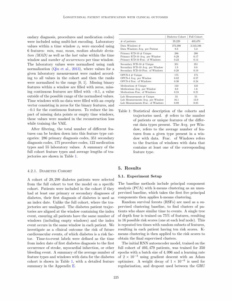
After filtering, the total number of different fea-tures can be broken down into this feature type cat-egories: 286 primary diagnosis codes, 351 secondarydiagnosis codes, 175 procedure codes, 122 medicationtypes and 55 laboratory values. A summary of thefull cohort feature types and average lengths of tra-jectories are shown in Table 1.

4.2.1. Diabetes Cohort

A cohort of 29, 299 diabetes patients were selectedfrom the full cohort to test the model on a specificcohort. Patients were included in the cohort if theyhad at least one primary or secondary diagnoses ofdiabetes, their first diagnosis of diabetes is used asan index date. Unlike the full cohort, where the tra-jectories are unaligned. The diabetes patient trajec-tories are aligned at the window containing the indexevent, ensuring all patients have the same number ofwindows (including empty windows) and the indexevent occurs in the same window in each patient. Weinvestigate as a clinical outcome the risk of futurecardiovascular events, of which diabetes is a risk fac-tor. Time-to-event labels were defined as the timefrom index date of first diabetes diagnosis to the firstoccurrence of stroke, myocardial infarction, or otherbleeding event. A summary of the average number offeature types and windows with data for the diabetescohort is shown in Table 1, with a detailed featuresummary in the Appendix E.

Diabetes Cohort Full Cohort

# of patients 29,229 493,470

Data Windows # 272,390 2,543,106Data Windows Avg. per Patient 9.3 5.2

Primary ICD-10 # Unique 286 286Primary ICD-10 Avg. per Window 0.29 0.17Primary ICD-10 Frac. of Windows 0.23 0.14

Secondary ICD-10 # Unique 351 351Secondary ICD-10 Avg. per Window 1.9 0.8Secondary ICD-10 Frac. of Windows 0.28 0.19

OPCS-4 # Unique 175 175OPCS-4 Avg. per Window 0.82 0.57OPCS-4 Frac. of Windows 0.30 0.24

Medications # Unique 122 122Medications Avg. per Window 3.0 1.6Medications Frac. of Windows 0.24 0.21

Lab Measurements # Unique 55 55Lab Measurements Avg. per Window 16.1 13.9Lab Measurements Frac. of Windows 0.89 0.85

Table 1: Statistical description of the cohorts andtrajectories used. # refers to the numberof patients or unique features of the differ-ent data types present. The Avg. per Win-dow, refers to the average number of fea-tures from a given type present in a win-dow with data. Frac. of Windows refersto the fraction of windows with data thatcontains at least one of the correspondingfeature type.

5. Results

5.1. Experiment Setup

The baseline methods include principal componentanalysis (PCA) with k-means clustering as an unsu-pervised baseline, which takes the first five principalcomponents then applies k-means clustering.

Random survival forests (RSFs) are used as a su-pervised clustering baseline, to find clusters of pa-tients who share similar time to events. A single treeof depth four is trained on 75% of features, resultingin 16 possible risk scores (one at each leaf node). Thisis repeated ten times with random subsets of features,resulting in each patient having ten risk scores. K-means clustering is then applied to the risk scores toobtain the final supervised clusters.

The initial RNN autoencoder model, trained on thefull cohort of 493, 479 patients, was trained for 350epochs with a batch size of 4, 096 and a learning rateof 2 × 10−3 using gradient descent with an Adamoptimiser. A weight decay of 1 × 10−6 is used forregularisation, and dropout used between the GRU

225


layers (p = 0.1). The output dimension of the fullyconnected encoder layers was 256, with the hiddenstate of the GRU having dimensions of 256. The pro-posed LPS-CO model, trained on the diabetes cohortof 29, 299 patients, was trained for 25 epochs with abatch size of 256 with the other parameters remain-ing the same. Hyperparamters are selected to ensurelosses are converging, although no formal optimisa-tion was applied. All models were built using Py-Torch. The model architecture is described in moredetail in Appendix B.

Three versions of the proposed LPS-CO model areused with different loss weights (Equation 1) for re-construction loss, wr, and outcome loss, wy: no out-come loss (wr = 0.5, wy = 0), no reconstruction loss(wr = 0, wy = 1), and both reconstruction and out-come loss (wr = 0.05, wy = 1), these weights arechosen to ensure the losses are of similar magnitudeswhen combined, they have not been optimised andare left to the user depending on model requirements.In all models the KL divergence loss weight, wkl, isset to 1 × 10−5 and the clustering loss weight is setto 0.25.

5.2. Synthetic Data Results

To validate the proposed model and evaluate thecombination of reconstruction and outcome loss, themodel was applied to the synthetic dataset. Thethree versions of the LPS-CO model with differentloss weights were trained on the synthetic data. Inaddition to the proposed model, PCA k-means wastrained as a baseline unsupervised clustering model,a random survival forest was trained as a baseline su-pervised clustering model, and an AC-TCP modelproposed by Lee and van der Schaar (2020) wastrained as a state-of-the-art comparison. All mod-els were trained two times, once to find three clustersand once to find six clusters.

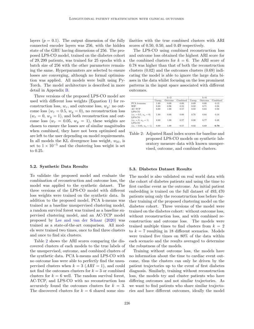
Table 2 shows the ARI scores comparing the dis-covered clusters of each models to the true labels ofthe unsupervised, outcome, and combined clusters ofthe synthetic data. PCA k-means and LPS-CO withno outcome loss were able to perfectly find the unsu-pervised clusters when k = 3 (ARI = 1), and couldnot find the outcomes clusters for k = 3 or combinedclusters for k = 6 well. The random survival forest,AC-TCP, and LPS-CO with no reconstruction lossaccurately found the outcomes clusters for k = 3.The discovered clusters for k = 6 shared some sim-

ilarities with the true combined clusters with ARIscores of 0.50, 0.50, and 0.49 respectively.

The LPS-CO using combined reconstruction lossand outcome loss obtained the highest ARI score forthe combined clusters for k = 6. The ARI score of0.78 was higher than that of both the reconstructionclusters (0.02) and the outcomes clusters (0.69) indi-cating the model is able to ignore the large data bi-ases in the data whilst focusing on the less prominentpatterns in the input space associated with differentoutcomes.

k=3 k=6Unsup. Outcome Combined Unsup. Outcome Combined

PCA k-means 1.00 0.00 0.00 0.69 0.08 0.13RSF 0.00 0.96 0.55 0.02 0.71 0.50AC-TCP 0.00 1.00 0.57 0.02 0.84 0.50LPS-CO(wr = 0.5, wy = 0) 1.00 0.00 0.00 0.76 0.04 0.10LPS-CO(wr = 0, wy = 1) 0.00 1.00 0.57 0.00 0.77 0.49LPS-CO(wr = 0.05, wy = 1) 0.00 1.00 0.57 0.02 0.69 0.78

Table 2: Adjusted Rand index scores for baseline andproposed LPS-CO models on synthetic lab-oratory measure data with known unsuper-vised, outcome, and combined clusters.

5.3. Diabetes Dataset Results

The model is also validated on real world data withthe cohort of diabetes patients and using the time tofirst cardiac event as the outcome. An initial patientembedding is trained on the full dataset of 493, 470patients using only the reconstruction loss before fur-ther training of the proposed clustering model on thediabetes cohort. Three versions of the model weretrained on the diabetes cohort: without outcome loss,without reconstruction loss, and with combined re-construction and outcome loss. The models weretrained multiple times to find clusters from k = 2to k = 7 resulting in 18 different scenarios. Modelswere trained five times on 80% of the data withineach scenario and the results averaged to determinethe robustness of the models.

Training without outcome loss, the models haveno information about the time to cardiac event out-come, thus the clusters can only be driven by thepatient trajectories up to the event of first diabetesdiagnosis. Similarly, training without reconstructionloss, the models try and cluster patients who havediffering outcomes and not similar trajectories. Aswe want to find patients who share similar trajecto-ries and have different outcomes, ideally the model

226


Clusters Recon.-Combined Outcome-Combined Recon.-Outcome2 0.07± 0.08 0.18± 0.11 0.06± 0.093 0.31± 0.22 0.30± 0.23 0.13± 0.164 0.10± 0.02 0.21± 0.11 0.07± 0.055 0.15± 0.02 0.22± 0.13 0.07± 0.036 0.14± 0.07 0.24± 0.16 0.09± 0.057 0.14± 0.05 0.27± 0.07 0.07± 0.02

Table 3: Adjusted Rand index scores between pairsof LPS-CO clusters from different lossweights, showing similarities between thediscovered clusters for each k.

with combined losses shares information with boththe clusters driven by the trajectories and the clus-ters driven by outcomes.

Table 3 shows the mean and standard deviationof ARI scores comparing clusters found using recon-struction loss with combined loss, outcome loss withcombined loss, and reconstruction loss with outcomeloss. The ARI scores between the reconstructionand outcome loss clusters are low (a maximum of0.13± 0.16 for k = 3), indicating little similarity be-tween the discovered clusters. This is as expecteddue to the differing focuses on trajectories and out-comes. The ARI scores between the combined clus-ters and both the reconstruction and outcome clus-ters are higher in all cases, showing the combinedloss model is learning from both trajectories and out-comes. The ARI scores between combined loss clus-ters and outcome loss clusters are generally higherthan the scores between combined loss clusters andreconstruction loss clusters, suggesting the combinedlosses focus more on the outcomes.

LPS-CO LPS-CO LPS-COClusters (wr = 0.5, wy = 0) (wr = 0, wy = 1) (wr = 0.05, wy = 1)2 345± 171 950± 793 825± 5143 766± 112 7483± 2691 5366± 25204 1169± 217 7779± 4773 4029± 47325 1900± 343 6637± 3846 2657± 8846 1190± 151 5958± 2129 7527± 30367 1961± 447 10770± 2367 8575± 1955

Table 4: Log rank test statistic between reconstruc-tion (wr = 0.5, wy = 0), outcome (wr = 0,wy = 1), and combined (wr = 0.05, wy =1) loss clusters, showing separation of out-comes between the discovered clusters foreach k.

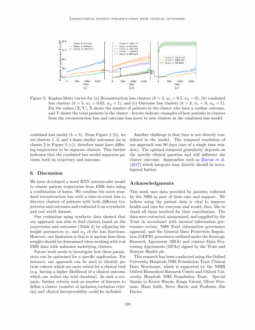
Figure 2 (a) and (c) show the KM curves for theclusters found using the reconstruction loss only, com-bined loss, and outcome loss only models for k = 3.

The curves estimate the time to first cardiac eventfor the patients in each cluster. We see that for re-construction loss only in Figure 2 (a) the curves areless separable, with the curves for the outcome lossonly in Figure 2 (c) most separable. Using combinedlosses in Figure 2 the separation of the KM curvesare between the two other models. This is quantifiedin Table 4 where the mean and standard deviation ofthe multivariate log rank test statistic can be seen fork = 2 to k = 7 for each model. In all cases, the teststatistic is highest for the outcome loss only model,indicating the highly differing KM curves, and low-est for the reconstruction loss only, indicating similarKM curves in each cluster. Again, the combined lossmodel is intermediate, showing it is combining bothoutcome and trajectory information.

Clusters Comb. 1 Comb. 2 Comb. 3 Comb. 4 Comb. 5Recon. 1 0.04 0.29 0.40 0.15 0.12Recon. 2 0.01 0.13 0.42 0.10 0.34Recon. 3 0.39 0.01 0.02 0.56 0.02Outcome 1 0.01 0.15 0.32 0.40 0.13Outcome 2 0.37 0.03 0.21 0.27 0.12Outcome 3 0.00 0.43 0.07 0.10 0.40

Table 5: The fraction of patients from each clusterof the combined loss model (k=5) in eachcluster of the reconstruction loss only andoutcome loss only models (k=3).

We also investigate how patients in clusters foundfrom trajectories (reconstruction loss only) and out-comes (outcome loss only) for small numbers of clus-ters (k = 3) split and are distributed through highernumber of clusters (k = 5) using a combined lossmodel. Table 5 shows the distributions of patientsfrom each of the clusters for k = 3 within the clustersfor the combined loss model using k = 5.

Two cases on how clusters of patients are split go-ing from k = 3 to k = 5 are highlighted. Patients incluster 2 using reconstruction loss only k = 3, are pri-marily assigned to clusters 3 (42%) and 5 (54%) fromthe combined loss model (k = 5). From Figure 2 (b)we can see clusters 3 and 5 have different outcomes,yet we know the patients share similar trajectoriesas they are assigned to the same clusters in the re-construction only model (k = 3). This indicates thecombined loss model is able to find clusters of patientswith similar trajectories, but different outcomes.

For the second case, patients in cluster 2 of the out-come loss only model (k = 3) are mainly distributedbetween clusters 1 (37%), 3 (21%), and 4 (27%) of the

227


Figure 2: Kaplan-Meier curves for (a) Reconstruction loss clusters (k = 3, wr = 0.5, wy = 0), (b) combinedloss clusters (k = 5, wr = 0.05, wy = 1), and (c) Outcome loss clusters (k = 3, wr = 0, wy = 1).For the values (X/Y), X shows the number of patients in the cluster who have a cardiac outcome,and Y shows the total patients in the cluster. Arrows indicate examples of how patients in clustersfrom the reconstruction loss and outcome loss move to new clusters in the combined loss model.

combined loss model (k = 5). From Figure 2 (b), wesee clusters 1, 3, and 4 share similar outcomes (as incluster 2 in Figure 2 (c)), therefore must have differ-ing trajectories to be separate clusters. This furtherindicates that the combined loss model separates pa-tients both on trajectory and outcome.

6. Discussion

We have developed a novel RNN autoencoder modelto cluster patient trajectories from EHR data usinga combination of losses. We combine the more stan-dard reconstruction loss with a time-to-event loss todiscover clusters of patients with both different tra-jectories and outcomes and evaluated it on a syntheticand real world dataset.Our evaluation using synthetic data showed that

our approach was able to find clusters based on thetrajectories and outcomes (Table 2) by adjusting theweight parameters wr and wy of the loss functions.However, one limitation is that it is unclear how theseweights should be determined when working with realEHR data with unknown underlying clusters.Future work needs to investigate how these param-

eters can be optimised for a specific application. Forinstance, our approach can be used to identify pa-tient cohorts which are more suited for a clinical trial(e.g. having a higher likelihood of a clinical outcomewhich can reduce the trial duration). In such a sce-nario, further criteria such as number of features todefine a cluster (number of inclusion/exclusion crite-ria) and clinical interpretability could be included.

Another challenge is that time is not directly con-sidered in the model. The temporal resolution ofour approach was 90 days (size of a single time win-dow). The optimal temporal granularity depends onthe specific clinical question and will influence thecluster outcome. Approaches such as Baytas et al.(2017) which integrate time directly should be inves-tigated further.

Acknowledgments

This work uses data provided by patients collectedby the NHS as part of their care and support. Webelieve using the patient data is vital to improvehealth and care for everyone and would, thus, like tothank all those involved for their contribution. Thedata were extracted, anonymised, and supplied by theTrust in accordance with internal information gov-ernance review, NHS Trust information governanceapproval, and the General Data Protection Regula-tion (GDPR) procedures outlined under the StrategicResearch Agreement (SRA) and relative Data Pro-cessing Agreements (DPAs) signed by the Trust andSensyne Health plc.

This research has been conducted using the OxfordUniversity Hospitals NHS Foundation Trust ClinicalData Warehouse, which is supported by the NIHROxford Biomedical Research Centre and Oxford Uni-versity Hospitals NHS Foundation Trust. Specialthanks to Kerrie Woods, Kinga Varnai, Oliver Free-man, Hizni Salih, Steve Harris and Professor JimDavies.

228


References

Sameer Ather, Leif E Peterson, Vijay Divakaran,Anita Deswal, Biykem Bozkurt, and Douglas LMann. Unsupervised cluster analysis and mortalityrisk in the digitalis investigation group (DIG) trialof heart failure. In 2009 International Joint Con-ference on Neural Networks, pages 207–212, 2009.

Inci M. Baytas, Cao Xiao, Xi Zhang, Fei Wang,Anil K. Jain, and Jiayu Zhou. Patient Subtypingvia Time-Aware LSTMNetworks. In Proceedings ofthe 23rd ACM SIGKDD International Conferenceon Knowledge Discovery and Data Mining, pages65–74, New York, NY, USA, 2017.

Ghalib A. Bello, Timothy J. W. Dawes, JinmingDuan, Carlo Biffi, Antonio de Marvao, Luke S.G. E. Howard, J. Simon R. Gibbs, Martin R.Wilkins, Stuart A. Cook, Daniel Rueckert, and De-clan P. O’Regan. Deep-learning cardiac motionanalysis for human survival prediction. Nature Ma-chine Intelligence, 1(2):95–104, 2019.

D J Berndt and J Clifford. Using dynamic time warp-ing to find patterns in time series, 1994.

P-R Burgel, J-L Paillasseur, D Caillaud, I Tillie-Leblond, P Chanez, R Escamilla, I Court-Fortune,T Perez, P Carre, N Roche, and Initiatives BPCOScientific Committee. Clinical COPD phenotypes:a novel approach using principal component andcluster analyses. Eur. Respir. J., 36(3):531–539,2010.

Oliver Carr, Stojan Jovanovic, Luca Albergante,Fernando Andreotti, Robert Durichen, NadiaLipunova, Janie Baxter, Rabia Khan, and Ben-jamin Irving. Deep Semi-Supervised EmbeddedClustering (DSEC) for Stratification of Heart Fail-ure Patients. In Healthcare Systems, PopulationHealth, and the Role of Health-Tech, InternationalConference on Machine Learning, 2020.

Jose Castela Forte, Galiya Yeshmagambetova, Mau-reen L. van der Grinten, Bart Hiemstra, ThomasKaufmann, Ruben J. Eck, Frederik Keus, Anne H.Epema, Marco A. Wiering, and Iwan C.C. van derHorst. Identifying and characterizing high-riskclusters in a heterogeneous ICU population withdeep embedded clustering. Scientific Reports, 11(1):1–12, 2021.

Kyunghyun Cho, Bart Van Merrienboer, Caglar Gul-cehre, Dzmitry Bahdanau, Fethi Bougares, HolgerSchwenk, and Yoshua Bengio. Learning phrase rep-resentations using RNN encoder-decoder for sta-tistical machine translation. EMNLP 2014 - 2014Conference on Empirical Methods in Natural Lan-guage Processing, Proceedings of the Conference,pages 1724–1734, 2014.

Johann de Jong, Mohammad Asif Emon, Ping Wu,Reagon Karki, Meemansa Sood, Patrice Godard,Ashar Ahmad, Henri Vrooman, Martin Hofmann-Apitius, and Holger Frohlich. Deep learning forclustering of multivariate clinical patient trajecto-ries with missing values. GigaScience, 8(11):1–14,2019.

V Ehrenstein, H Kharrazi, and H Lehmann. Ob-taining Data From Electronic Health Records. InR E Gliklich, M B Leavy, and N A Dreyer, editors,Tools and Technologies for Registry Interoperabil-ity, Registries for Evaluating Patient Outcomes: AUser’s Guide, chapter 4. Agency for Healthcare Re-search and Quality (US), Rockville (MD), 3rd edi-tio edition, 2019.

Johann Hammer, Stuart Howell, Peter Bytzer,Michael Horowitz, and Nicholas J Talley. Symptomclustering in subjects with and without diabetesmellitus: a population-based study of 15,000 aus-tralian adults. Am. J. Gastroenterol., 98(2):391–398, 2003.

David P Harrington and Thomas R Fleming. A classof rank test procedures for censored survival data.Biometrika, 69(3):553–566, 1982.

Asa K Hedman, Camilla Hage, Anil Sharma,Mary Julia Brosnan, Leonard Buckbinder, Li-MingGan, Sanjiv J Shah, Cecilia M Linde, Erwan Donal,Jean-Claude Daubert, Anders Malarstig, DanielZiemek, and Lars Lund. Identification of novelpheno-groups in heart failure with preserved ejec-tion fraction using machine learning. Heart, 106(5):342–349, 2020.

G E Hinton and R R Salakhutdinov. Reducing thedimensionality of data with neural networks. Sci-ence, 313(5786):504–507, 2006.

Sepp Hochreiter and Jurgen Schmidhuber. LongShort-Term Memory. Neural Computation, 9(8):1735–1780, 1997.

229


E L Kaplan and Paul Meier. Nonparametric estima-tion from incomplete observations. J. Am. Stat.Assoc., 53(282):457–481, 1958.

Diederik P. Kingma and MaxWelling. Auto-encodingvariational bayes. 2nd International Conference onLearning Representations, ICLR 2014 - ConferenceTrack Proceedings, pages 1–14, 2014.

Isotta Landi, Benjamin S. Glicksberg, Hao Chih Lee,Sarah Cherng, Giulia Landi, Matteo Danieletto,Joel T. Dudley, Cesare Furlanello, and RiccardoMiotto. Deep representation learning of electronichealth records to unlock patient stratification atscale. npj Digital Medicine, 3(1):1–11, 2020.

Changhee Lee and Mihaela van der Schaar. Temporalphenotyping using deep predictive clustering of dis-ease progression. 37th International Conference onMachine Learning, ICML 2020, pages 5723–5733,2020.

Changhee Lee, Jem Rashbass, and Mihaela Van DerSchaar. Outcome-Oriented Deep Temporal Pheno-typing of Disease Progression. IEEE Transactionson Biomedical Engineering, pages 1–1, 2020.

Gavin A. Lewis, Erik B. Schelbert, Simon G.Williams, Colin Cunnington, Fozia Ahmed,Theresa A. McDonagh, and Christopher A. Miller.Biological Phenotypes of Heart Failure With Pre-served Ejection Fraction. Journal of the AmericanCollege of Cardiology, 70(17):2186–2200, 2017.

Naveen Sai Madiraju, Seid M. Sadat, Dimitry Fisher,and Homa Karimabadi. Deep Temporal Cluster-ing : Fully Unsupervised Learning of Time-DomainFeatures. arXiv, pages 1–11, 2018.

Riccardo Miotto, Li Li, Brian A Kidd, and Joel TDudley. Deep Patient: An Unsupervised Repre-sentation to Predict the Future of Patients fromthe Electronic Health Records. Scientific Reports,6, 2016.

Wendy C Moore, Deborah A Meyers, Sally E Wenzel,W Gerald Teague, Huashi Li, Xingnan Li, RalphD’Agostino, Jr, Mario Castro, Douglas Curran-Everett, Anne M Fitzpatrick, Benjamin Gaston,Nizar N Jarjour, Ronald Sorkness, William JCalhoun, Kian Fan Chung, Suzy A A Comhair,Raed A Dweik, Elliot Israel, Stephen P Peters,William W Busse, Serpil C Erzurum, Eugene R

Bleecker, and National Heart, Lung, and Blood In-stitute’s Severe Asthma Research Program. Iden-tification of asthma phenotypes using cluster anal-ysis in the severe asthma research program. Am.J. Respir. Crit. Care Med., 181(4):315–323, 2010.

Sarah Mullin, Jaroslaw Zola, Robert Lee, JinweiHu, Brianne MacKenzie, Arlen Brickman, GabrielAnaya, Shyamashree Sinha, Angie Li, and Peter LElkin. Longitudinal K-Means approaches to clus-tering and analyzing EHR opioid use trajectoriesfor clinical subtypes. J. Biomed. Inform., page103889, 2021.

Xing Qiu, Hulin Wu, and Rui Hu. The impact ofquantile and rank normalization procedures on thetesting power of gene differential expression analy-sis. BMC Bioinformatics, 14(1):1–10, 2013.

Antonio Sarrıa-Santamera, Binur Orazumbekova,Tilektes Maulenkul, Abduzhappar Gaipov, andKuralay Atageldiyeva. The identification of dia-betes mellitus subtypes applying cluster analysistechniques: A systematic review. Int. J. Environ.Res. Public Health, 17(24), 2020.

Benjamin Shickel, Patrick James Tighe, Azra Biho-rac, and Parisa Rashidi. Deep EHR: A Survey ofRecent Advances in Deep Learning Techniques forElectronic Health Record (EHR) Analysis. IEEEJournal of Biomedical and Health Informatics, 22(5):1589–1604, 2018.

Susan E. Spratt, Katherine Pereira, Bradi B.Granger, Bryan C. Batch, Matthew Phelan,Michael Pencina, Marie Lynn Miranda, EbonyBoulware, Joseph E. Lucas, Charlotte L. Nel-son, Benjamin Neely, Benjamin A. Goldstein,Pamela Barth, Rachel L. Richesson, Isaretta L.Riley, Leonor Corsino, Eugenia R. McPeek Hinz,Shelley Rusincovitch, Jennifer Green, Anna BethBarton, Carly Kelley, Kristen Hyland, MonicaTang, Amanda Elliott, Ewa Ruel, Alexander Clark,Melanie Mabrey, Kay Lyn Morrissey, Jyothi Rao,Beatrice Hong, Marjorie Pierre-Louis, KatherineKelly, and Nicole Jelesoff. Assessing electronichealth record phenotypes against gold-standard di-agnostic criteria for diabetes mellitus. Journal ofthe American Medical Informatics Association, 24(1):121–128, 2017.

Laurens van der Maaten and Geoffrey Hinton. Visu-alizing data using t-SNE. J. Mach. Learn. Res., 9(86):2579–2605, 2008.

230


Pascal Vincent, Hugo Larochelle, Isabelle Lajoie,Yoshua Bengio, and Pierre-Antoine Manzagol.Stacked denoising autoencoders: Learning usefulrepresentations in a deep network with a local de-noising criterion. J. Mach. Learn. Res., 11(110):3371–3408, 2010.

Junyuan Xie, Ross Girshick, and Ali Farhadi. Un-supervised deep embedding for clustering analysis.33rd International Conference on Machine Learn-ing, ICML 2016, 1:740–749, 2016.

Jinghe Zhang, Kamran Kowsari, James H. Harri-son, Jennifer M. Lobo, and Laura E. Barnes. Pa-tient2Vec: A Personalized Interpretable Deep Rep-resentation of the Longitudinal Electronic HealthRecord. IEEE Access, 6:65333–65346, 2018.

Xi Zhang, Jingyuan Chou, Jian Liang, Cao Xiao,Yize Zhao, Harini Sarva, Claire Henchcliffe, and FeiWang. Data-Driven Subtyping of Parkinson’s Dis-ease Using Longitudinal Clinical Records: A Co-hort Study. Scientific Reports, 9(1):1–12, 2019.

Zihao Zhu, Changchang Yin, Buyue Qian, Yu Cheng,Jishang Wei, and Fei Wang. Measuring patientsimilarities via a deep architecture with medicalconcept embedding. In 2016 IEEE 16th Interna-tional Conference on Data Mining (ICDM), pages749–758, 2016.

Appendix A. Generating SyntheticData

When generating the synthetic clusters, we chose thevariance of unsupervised clusters such that it waslarger than that of combined clusters. This ensuredthat they were favoured by purely unsupervised clus-tering methods (e.g., PCA k-means or DEC), whereassemi and supervised methods (e.g., RSF, AC-TCP)are expected to find the simulated outcome clusters.However, the latter disregard different patient tra-jectories in the input space that lead to similar out-comes. In order to show that — depending on theweighting of the loss functions — our proposed modelcan also recover the specific trajectories that lead tooutcomes, we further split the outcome clusters intosubgroups that shared the same outcome distributionbut a different covariate distribution.

The synthetic data is generated with the followingsteps:

• The number of noise clusters, Knoise = 3,is specified along with the number of syn-thetic features which contribute to these clus-ters, Nnoise = 200. Features are sampled fromisotropic Gaussian distributions with standarddeviation Cstd = 3 and with cluster centroidsgenerated at random within a bounding box,(centremin = −10, centremax = −10). The gen-erated features are continuous and represent syn-thetic laboratory measures. In order to gen-erate synthetic binary features (eg. diagno-sis codes), synthetic continuous features can bepassed through a min max scaler and rounded tozero or one.

• The number of outcome clusters, Koutcome = 3,is specified along with minimum and maximumtime to events (TTEmin = 10, TTEmax =10, 000). The time to events are generated bysampling from exponential distributions with thescale of the distribution for each cluster oneof the values log-spaced between TTEmin andTTEmax with Koutcome steps. Censoring ofevents is sampled randomly from a uniform dis-tribution (p = 0.5), with all time to events overa maximum threshold (2, 000) set to this maxvalue and censored.

• The number of combined clusters, Kcombined =6, is set to twice the value of Koutcome andthe number of synthetic features which corre-

231


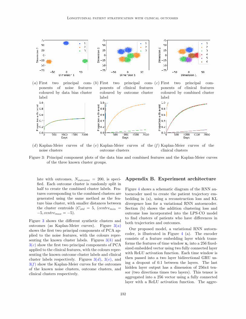
(a) First two principal com-ponents of noise featurescoloured by data bias clusterlabel

(b) First two principal com-ponents of clinical featurescoloured by outcome clusterlabel

(c) First two principal com-ponents of clinical featurescoloured by combined clusterlabel

(d) Kaplan-Meier curves of thenoise clusters

(e) Kaplan-Meier curves of theoutcome clusters

(f ) Kaplan-Meier curves of theclinical clusters

Figure 3: Principal component plots of the data bias and combined features and the Kaplan-Meier curvesof the three known cluster groups.

late with outcomes, Noutcome = 200, is speci-fied. Each outcome cluster is randomly split inhalf to create the combined cluster labels. Fea-tures corresponding to the combined clusters aregenerated using the same method as the fea-ture bias cluster, with smaller distances betweenthe cluster centroids (Cstd = 5, (centremin =−5, centremax = −5).

Figure 3 shows the different synthetic clusters andoutcomes (as Kaplan-Meier curves). Figure 3(a)shows the first two principal components of PCA ap-plied to the noise features, with the colours repre-senting the known cluster labels. Figures 3(b) and3(c) show the first two principal components of PCAapplied to the clinical features, with the colours repre-senting the known outcome cluster labels and clinicalcluster labels respectively. Figures 3(d), 3(e), and3(f ) show the Kaplan-Meier curves for the outcomesof the known noise clusters, outcome clusters, andclinical clusters respectively.

Appendix B. Experiment architecture

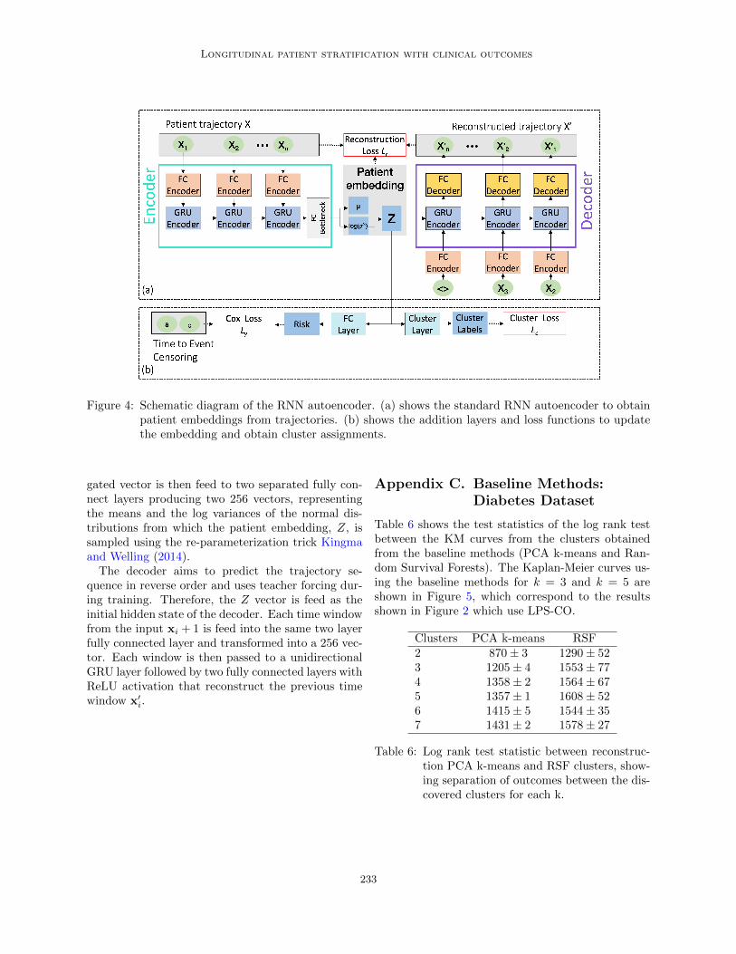
Figure 4 shows a schematic diagram of the RNN au-toencoder used to create the patient trajectory em-bedding in (a), using a reconstruction loss and KLdivergence loss for a variational RNN autoencoder.Section (b) shows the addition clustering loss andoutcome loss incorporated into the LPS-CO modelto find clusters of patients who have differences inboth trajectories and outcomes.

Our proposed model, a variational RNN autoen-coder, is illustrated in Figure 4 (a). The encoderconsists of a feature embedding layer which trans-forms the features of time window xi into a 256 fixed-sized embedded vector using two fully connected layerwith ReLU activation function. Each time window isthen passed into a two layer bidirectional GRU us-ing a dropout of 0.1 between the layers. The lasthidden layer output has a dimension of 256x4 ten-sor (two directions times two layers). This tensor isaggregated into a 256 vector using a fully connectedlayer with a ReLU activation function. The aggre-

232


Figure 4: Schematic diagram of the RNN autoencoder. (a) shows the standard RNN autoencoder to obtainpatient embeddings from trajectories. (b) shows the addition layers and loss functions to updatethe embedding and obtain cluster assignments.

gated vector is then feed to two separated fully con-nect layers producing two 256 vectors, representingthe means and the log variances of the normal dis-tributions from which the patient embedding, Z, issampled using the re-parameterization trick Kingmaand Welling (2014).The decoder aims to predict the trajectory se-

quence in reverse order and uses teacher forcing dur-ing training. Therefore, the Z vector is feed as theinitial hidden state of the decoder. Each time windowfrom the input xi + 1 is feed into the same two layerfully connected layer and transformed into a 256 vec-tor. Each window is then passed to a unidirectionalGRU layer followed by two fully connected layers withReLU activation that reconstruct the previous timewindow x′

i.

Appendix C. Baseline Methods:Diabetes Dataset

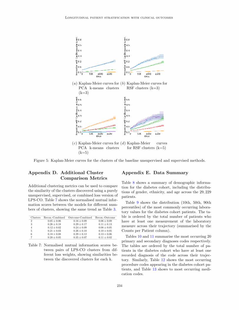
Table 6 shows the test statistics of the log rank testbetween the KM curves from the clusters obtainedfrom the baseline methods (PCA k-means and Ran-dom Survival Forests). The Kaplan-Meier curves us-ing the baseline methods for k = 3 and k = 5 areshown in Figure 5, which correspond to the resultsshown in Figure 2 which use LPS-CO.

Clusters PCA k-means RSF2 870± 3 1290± 523 1205± 4 1553± 774 1358± 2 1564± 675 1357± 1 1608± 526 1415± 5 1544± 357 1431± 2 1578± 27

Table 6: Log rank test statistic between reconstruc-tion PCA k-means and RSF clusters, show-ing separation of outcomes between the dis-covered clusters for each k.

233


(a) Kaplan-Meier curves forPCA k-means clusters(k=3)

(b) Kaplan-Meier curves forRSF clusters (k=3)

(c) Kaplan-Meier curves forPCA k-means clusters(k=5)

(d) Kaplan-Meier curvesfor RSF clusters (k=5)

Figure 5: Kaplan-Meier curves for the clusters of the baseline unsupervised and supervised methods.

Appendix D. Additional ClusterComparison Metrics

Additional clustering metrics can be used to comparethe similarity of the clusters discovered using a purelyunsupervised, supervised, or combined loss version ofLPS-CO. Table 7 shows the normalised mutual infor-mation scores between the models for different num-bers of clusters, showing the same trend as Table 3.

Clusters Recon.-Combined Outcome-Combined Recon.-Outcome2 0.05± 0.06 0.16± 0.09 0.06± 0.093 0.26± 0.18 0.29± 0.17 0.11± 0.134 0.12± 0.02 0.24± 0.09 0.08± 0.055 0.21± 0.03 0.26± 0.10 0.10± 0.056 0.18± 0.08 0.29± 0.12 0.13± 0.067 0.20± 0.05 0.35± 0.07 0.11± 0.02

Table 7: Normalised mutual information scores be-tween pairs of LPS-CO clusters from dif-ferent loss weights, showing similarities be-tween the discovered clusters for each k.

Appendix E. Data Summary

Table 8 shows a summary of demographic informa-tion for the diabetes cohort, including the distribu-tions of gender, ethnicity, and age across the 29, 229patients.

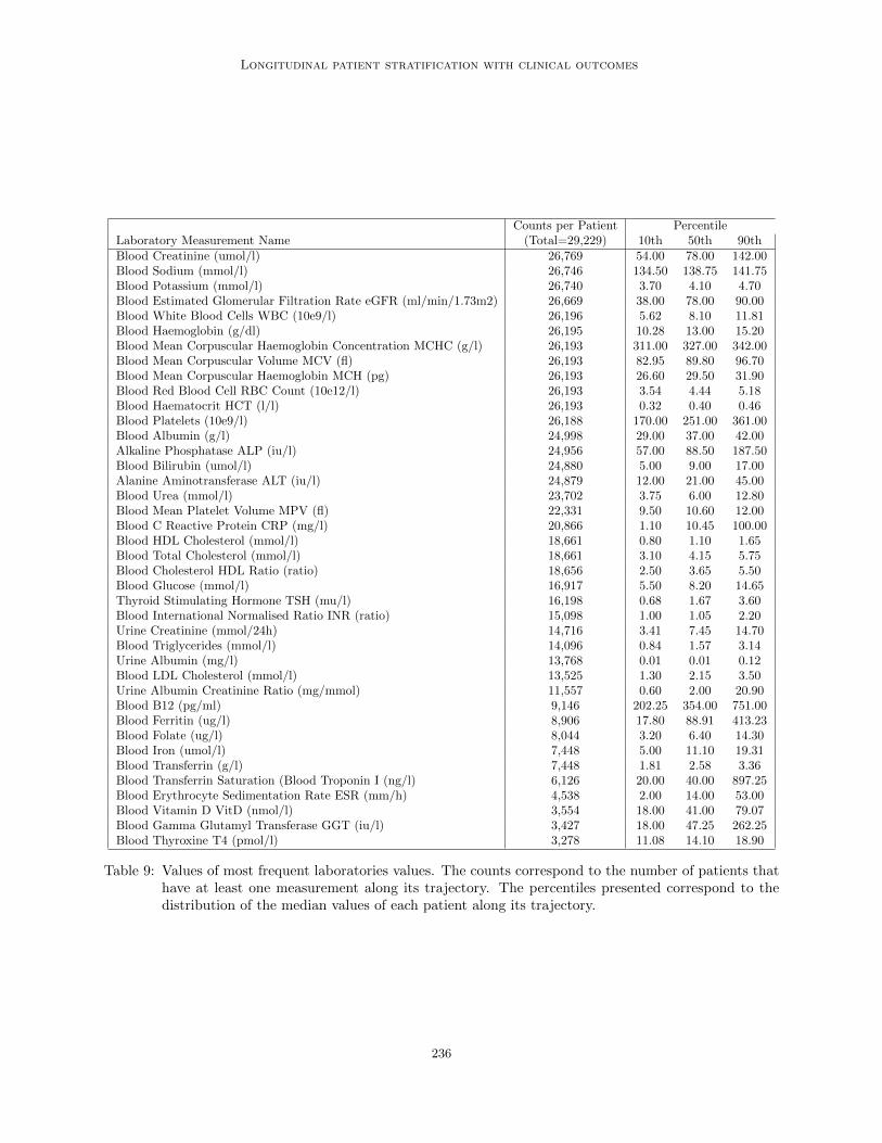
Table 9 shows the distribution (10th, 50th, 90thpercentiles) of the most commonly occurring labora-tory values for the diabetes cohort patients. The ta-ble is ordered by the total number of patients whohave at least one measurement of the laboratorymeasure across their trajectory (summarised by theCounts per Patient column).

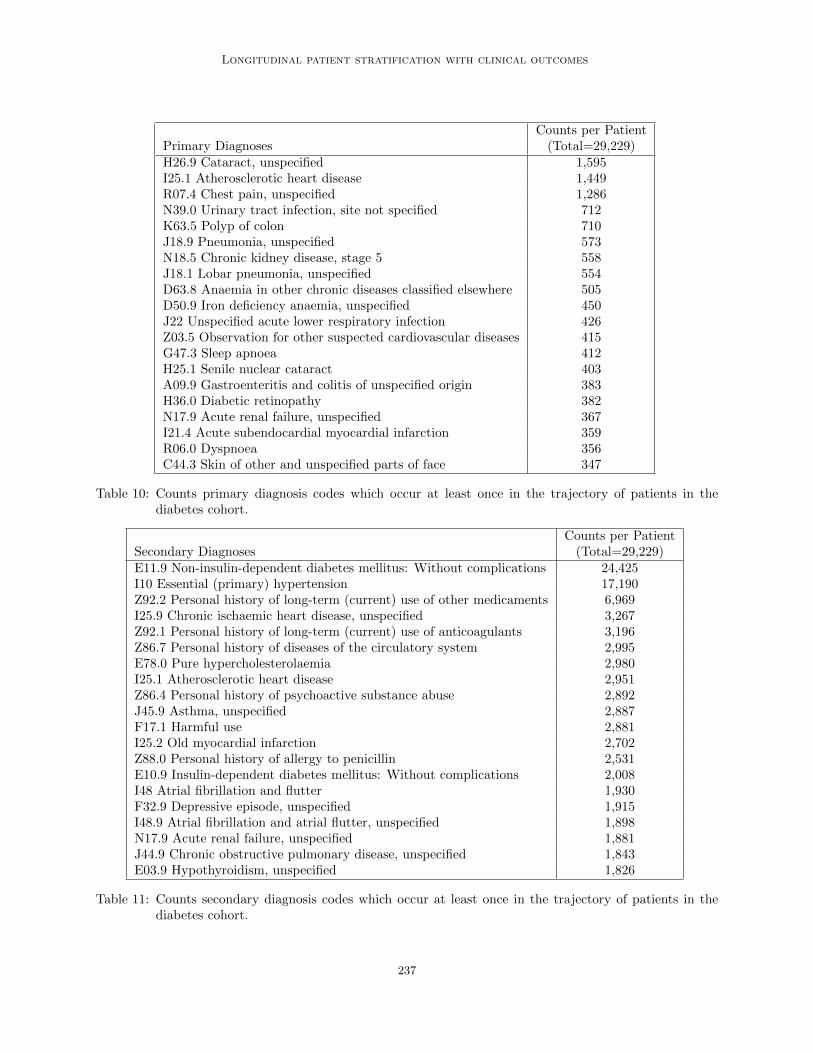
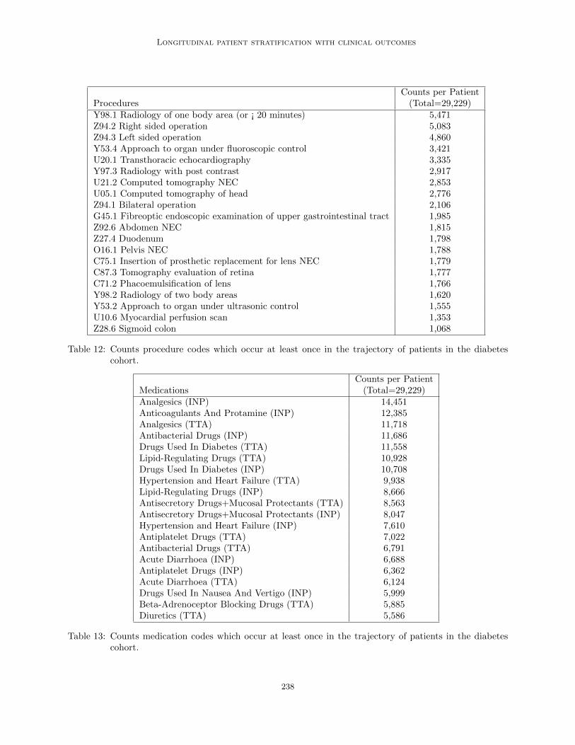
Tables 10 and 11 summarise the most occurring 20primary and secondary diagnoses codes respectively.The tables are ordered by the total number of pa-tients in the diabetes cohort who have at least onerecorded diagnosis of the code across their trajec-tory. Similarly, Table 12 shows the most occurringprocedure codes appearing in the diabetes cohort pa-tients, and Table 13 shows to most occurring medi-cation codes.

234


GenderMale Female Unknown16,824 12,403 2

EthnicityWhite British Not Stated Other

20,271 5,256 3,702

Age10th 50th 90th46.84 69.04 84.82

Table 8: Summary of demographic information of thediabetes cohort. Counts of gender, ethnic-ity, and percentiles of age are shown.

235


Counts per Patient PercentileLaboratory Measurement Name (Total=29,229) 10th 50th 90thBlood Creatinine (umol/l) 26,769 54.00 78.00 142.00Blood Sodium (mmol/l) 26,746 134.50 138.75 141.75Blood Potassium (mmol/l) 26,740 3.70 4.10 4.70Blood Estimated Glomerular Filtration Rate eGFR (ml/min/1.73m2) 26,669 38.00 78.00 90.00Blood White Blood Cells WBC (10e9/l) 26,196 5.62 8.10 11.81Blood Haemoglobin (g/dl) 26,195 10.28 13.00 15.20Blood Mean Corpuscular Haemoglobin Concentration MCHC (g/l) 26,193 311.00 327.00 342.00Blood Mean Corpuscular Volume MCV (fl) 26,193 82.95 89.80 96.70Blood Mean Corpuscular Haemoglobin MCH (pg) 26,193 26.60 29.50 31.90Blood Red Blood Cell RBC Count (10e12/l) 26,193 3.54 4.44 5.18Blood Haematocrit HCT (l/l) 26,193 0.32 0.40 0.46Blood Platelets (10e9/l) 26,188 170.00 251.00 361.00Blood Albumin (g/l) 24,998 29.00 37.00 42.00Alkaline Phosphatase ALP (iu/l) 24,956 57.00 88.50 187.50Blood Bilirubin (umol/l) 24,880 5.00 9.00 17.00Alanine Aminotransferase ALT (iu/l) 24,879 12.00 21.00 45.00Blood Urea (mmol/l) 23,702 3.75 6.00 12.80Blood Mean Platelet Volume MPV (fl) 22,331 9.50 10.60 12.00Blood C Reactive Protein CRP (mg/l) 20,866 1.10 10.45 100.00Blood HDL Cholesterol (mmol/l) 18,661 0.80 1.10 1.65Blood Total Cholesterol (mmol/l) 18,661 3.10 4.15 5.75Blood Cholesterol HDL Ratio (ratio) 18,656 2.50 3.65 5.50Blood Glucose (mmol/l) 16,917 5.50 8.20 14.65Thyroid Stimulating Hormone TSH (mu/l) 16,198 0.68 1.67 3.60Blood International Normalised Ratio INR (ratio) 15,098 1.00 1.05 2.20Urine Creatinine (mmol/24h) 14,716 3.41 7.45 14.70Blood Triglycerides (mmol/l) 14,096 0.84 1.57 3.14Urine Albumin (mg/l) 13,768 0.01 0.01 0.12Blood LDL Cholesterol (mmol/l) 13,525 1.30 2.15 3.50Urine Albumin Creatinine Ratio (mg/mmol) 11,557 0.60 2.00 20.90Blood B12 (pg/ml) 9,146 202.25 354.00 751.00Blood Ferritin (ug/l) 8,906 17.80 88.91 413.23Blood Folate (ug/l) 8,044 3.20 6.40 14.30Blood Iron (umol/l) 7,448 5.00 11.10 19.31Blood Transferrin (g/l) 7,448 1.81 2.58 3.36Blood Transferrin Saturation (Blood Troponin I (ng/l) 6,126 20.00 40.00 897.25Blood Erythrocyte Sedimentation Rate ESR (mm/h) 4,538 2.00 14.00 53.00Blood Vitamin D VitD (nmol/l) 3,554 18.00 41.00 79.07Blood Gamma Glutamyl Transferase GGT (iu/l) 3,427 18.00 47.25 262.25Blood Thyroxine T4 (pmol/l) 3,278 11.08 14.10 18.90

Table 9: Values of most frequent laboratories values. The counts correspond to the number of patients thathave at least one measurement along its trajectory. The percentiles presented correspond to thedistribution of the median values of each patient along its trajectory.

236


Counts per PatientPrimary Diagnoses (Total=29,229)H26.9 Cataract, unspecified 1,595I25.1 Atherosclerotic heart disease 1,449R07.4 Chest pain, unspecified 1,286N39.0 Urinary tract infection, site not specified 712K63.5 Polyp of colon 710J18.9 Pneumonia, unspecified 573N18.5 Chronic kidney disease, stage 5 558J18.1 Lobar pneumonia, unspecified 554D63.8 Anaemia in other chronic diseases classified elsewhere 505D50.9 Iron deficiency anaemia, unspecified 450J22 Unspecified acute lower respiratory infection 426Z03.5 Observation for other suspected cardiovascular diseases 415G47.3 Sleep apnoea 412H25.1 Senile nuclear cataract 403A09.9 Gastroenteritis and colitis of unspecified origin 383H36.0 Diabetic retinopathy 382N17.9 Acute renal failure, unspecified 367I21.4 Acute subendocardial myocardial infarction 359R06.0 Dyspnoea 356C44.3 Skin of other and unspecified parts of face 347

Table 10: Counts primary diagnosis codes which occur at least once in the trajectory of patients in thediabetes cohort.

Counts per PatientSecondary Diagnoses (Total=29,229)E11.9 Non-insulin-dependent diabetes mellitus: Without complications 24,425I10 Essential (primary) hypertension 17,190Z92.2 Personal history of long-term (current) use of other medicaments 6,969I25.9 Chronic ischaemic heart disease, unspecified 3,267Z92.1 Personal history of long-term (current) use of anticoagulants 3,196Z86.7 Personal history of diseases of the circulatory system 2,995E78.0 Pure hypercholesterolaemia 2,980I25.1 Atherosclerotic heart disease 2,951Z86.4 Personal history of psychoactive substance abuse 2,892J45.9 Asthma, unspecified 2,887F17.1 Harmful use 2,881I25.2 Old myocardial infarction 2,702Z88.0 Personal history of allergy to penicillin 2,531E10.9 Insulin-dependent diabetes mellitus: Without complications 2,008I48 Atrial fibrillation and flutter 1,930F32.9 Depressive episode, unspecified 1,915I48.9 Atrial fibrillation and atrial flutter, unspecified 1,898N17.9 Acute renal failure, unspecified 1,881J44.9 Chronic obstructive pulmonary disease, unspecified 1,843E03.9 Hypothyroidism, unspecified 1,826

Table 11: Counts secondary diagnosis codes which occur at least once in the trajectory of patients in thediabetes cohort.

237


Counts per PatientProcedures (Total=29,229)Y98.1 Radiology of one body area (or ¡ 20 minutes) 5,471Z94.2 Right sided operation 5,083Z94.3 Left sided operation 4,860Y53.4 Approach to organ under fluoroscopic control 3,421U20.1 Transthoracic echocardiography 3,335Y97.3 Radiology with post contrast 2,917U21.2 Computed tomography NEC 2,853U05.1 Computed tomography of head 2,776Z94.1 Bilateral operation 2,106G45.1 Fibreoptic endoscopic examination of upper gastrointestinal tract 1,985Z92.6 Abdomen NEC 1,815Z27.4 Duodenum 1,798O16.1 Pelvis NEC 1,788C75.1 Insertion of prosthetic replacement for lens NEC 1,779C87.3 Tomography evaluation of retina 1,777C71.2 Phacoemulsification of lens 1,766Y98.2 Radiology of two body areas 1,620Y53.2 Approach to organ under ultrasonic control 1,555U10.6 Myocardial perfusion scan 1,353Z28.6 Sigmoid colon 1,068

Table 12: Counts procedure codes which occur at least once in the trajectory of patients in the diabetescohort.

Counts per PatientMedications (Total=29,229)Analgesics (INP) 14,451Anticoagulants And Protamine (INP) 12,385Analgesics (TTA) 11,718Antibacterial Drugs (INP) 11,686Drugs Used In Diabetes (TTA) 11,558Lipid-Regulating Drugs (TTA) 10,928Drugs Used In Diabetes (INP) 10,708Hypertension and Heart Failure (TTA) 9,938Lipid-Regulating Drugs (INP) 8,666Antisecretory Drugs+Mucosal Protectants (TTA) 8,563Antisecretory Drugs+Mucosal Protectants (INP) 8,047Hypertension and Heart Failure (INP) 7,610Antiplatelet Drugs (TTA) 7,022Antibacterial Drugs (TTA) 6,791Acute Diarrhoea (INP) 6,688Antiplatelet Drugs (INP) 6,362Acute Diarrhoea (TTA) 6,124Drugs Used In Nausea And Vertigo (INP) 5,999Beta-Adrenoceptor Blocking Drugs (TTA) 5,885Diuretics (TTA) 5,586

Table 13: Counts medication codes which occur at least once in the trajectory of patients in the diabetescohort.

238

Documents

Longitudinal patient stratification of electronic health records