Embed Size (px)
Citation preview
The Association between the Uncertainty of Future Economic Benefits and Current R&D and Capital Expenditures:
Industry and Intertemporal Analyses
By
Eli Amir, Yanling Guan London Business School
Gilad Livne Cass School of Business
City University of London
June 2005
We thank Dan Weiss and seminar participants at Cardiff University, Lancaster University, London Business School, Singapore Management University, and Tel Aviv University for many useful comments. Address correspondence to Eli Amir, London Business School, +44-(0)207-2625050 (ext. 3182), [email protected].
1
The Association between the Uncertainty of Future Economic Benefits and Current R&D and Capital Expenditures:
Industry and Intertemporal Analyses
Abstract
Since 1974, R&D expenditures have been fully expensed when incurred partly because R&D activities are claimed to be associated with a high degree of uncertainty in future economic benefits. In this study, we estimate the association between R&D expenditures and capital expenditures (CAPEX) and the variance of future earnings per share and operating income. We show that R&D expenditures lead to higher volatility of future earnings than capital expenditures only in R&D-intensive industries, where industry R&D intensity is measured as the R&D-to-CAPEX ratio. We also find that the stronger association of R&D with uncertainty in future earnings is a recent phenomenon. Finally, we show that in industries that are relatively less dependent on R&D activities, the probability of recovering R&D expenditures is similar to that of capital expenditures. Overall, our results suggest that while some industries engage in a more innovative and uncertain R&D activities, R&D in other industries is less uncertain. These results suggest that the impact of R&D on future performance considerably varies across industries and time periods.
2
The Association between the Uncertainty of Future Economic Benefits and
Current R&D and Capital Expenditures: Industry and Intertemporal Analyses
1. Introduction
Accounting researchers have long debated whether the treatment of immediate expensing
of research and development (R&D) expenditures, required by Statement of Financial
Accounting Standard (SFAS) No. 2 is over-conservative. Specifically, to be accounted for as an
asset, an expenditure of interest should be related to future economic benefits, which are likely to
accrue to the reporting entity in future accounting periods. In particular, expenditures on
advertising, R&D, and training are expensed because it has been assumed that their link to future
benefits is tenuous. Capital expenditures, on the other hand, are incorporated into the balance
sheet as assets because it has been assumed that they generate future benefits to the firm with a
sufficiently high likelihood.
Prior literature has established that R&D expenditures are value relevant and that they
generate, on average, net future economic benefits. However, prior research also suggests that
R&D expenditures are associated with a high degree of variability in future economic benefits
more so than capital expenditures. This suggests that future benefits arising from R&D activities
are not sufficiently certain to meet the recognition criteria. Given the nature of R&D activities, it
is perhaps not surprising that, on average, R&D expenditures are more strongly associated with
uncertainty of future economic benefits than capital expenditures. Nonetheless, this result
deserves further scrutiny since R&D intensity varies significantly across industries and time.
While a large number of companies in many industries engage in R&D activities, the importance
3
of R&D and its effect on earnings, value and risk considerably varies over time, across
companies and in particular across industries.
The purpose of this study is therefore to examine whether the nature of the relation of R&D
expenditures and variability of future performance varies across industries and how it evolves
over time. Our first hypothesis is that the association between R&D and the variability of future
economic benefits varies across industries in a systematic and predictable manner. In particular,
we hypothesize that R&D is more associated with uncertainty in future benefits than capital
expenditures in industries in which R&D is a crucial driver of profitability. In industries in which
capital expenditures are the main driver of profitability and performance we would expect
weaker relation between R&D and variability of future benefits.
The second hypothesis advanced here relates to the possibility that a fundamental shift in
the way R&D projects are conducted has occurred in recent years. Specifically, the information
age revolution, which has witnessed an exponential increase in computing power coupled with
the development of efficient and rapid communication channels between the scientific
communities, entrepreneurs and companies, has introduced possibilities for innovation that were
not available before. A recent article in The Economist1 suggests, however, that its impact has
not been uniform across industries. Fast changing businesses whose success depends on the
ability to introduce genuinely new products have embraced the new frontiers by increasing
spending on R&D in the hope of finding one big winner. But, according to this article, despite
the increase in R&D, genuine innovations are fewer and far between. In other industries the
impact of the information age revolution has not been as dramatic since R&D is directed at
making relatively small improvements to existing products. In such industries, R&D expenditure
=================================================1 “Don’t laugh at gilded butterflies,” The Economist April 22nd 2004.
4
in recent years has not grown much and the rate of success has remained relatively unchanged.
Given the differential impact of information technology across industries, we conjecture that in
early years the relation between R&D and the variability of future performance was relatively
weak and quite similar across industries.
To examine these issues we collect a sample including all industries for which we could
obtain at least 1,000 firm-year observations with positive R&D expenditures. This is done to
ensure that we focus on industries with long “tradition” of expenditure on R&D. The nine sample
industries include traditional ones, such as Rubber & Plastics Products, as well as R&D-intensive
ones, such as Computers and Pharmaceuticals.
We define a measure of the relative importance of R&D to a firm’s success, which is based
on the ratio of annual R&D expenditures to annual capital expenditures (R&D-CAPEX ratio).
Industries that exhibit high R&D-CAPEX ratios are thought to be strongly reliant on R&D (e.g.,
Pharmaceuticals and Computers). Industries that exhibit low R&D-CAPEX ratios are less R&D
dependent (e.g., Metal Machinery and Rubber and Plastics).
We first assess what are the total benefits accruing to an investment of $1 in R&D. We find
that the undiscounted stream of benefits exceeds the original investment. This suggests that
investments in R&D are generally recoverable in our sample firms. This analysis also enables us
to assess the economic amortization rates of the implied R&D capital across the nine industries.
We find that useful life of R&D capital ranges between five and seven years. On this dimension
we observe little difference between traditional industries and R&D-intensive industries.
We then find that for industries with high R&D-CAPEX ratios, R&D exhibits greater
association with the variability of future benefits than capital expenditures. However, this result
is not obtained for industries with low R&D-CAPEX ratios. Incorporating measures of R&D
5
capital from the first analysis we also compare the association between R&D capital and property
plant and equipment (PPE) with variability of future performance. The results are similar to the
ones for R&D and capital expenditures. That is, R&D capital is more highly associated with
variability of future performance than PPE mainly for R&D-intensive firms.
Analyzing the evolution in the R&D-CAPEX ratio we note the beginning of an upward
trend in the mid 1980s in R&D-intensive industries, but no discernable trend for other industries.
Accordingly, we split our sample period into two sub-periods: 1972-1985 (early period) and
1986-1999 (late period). Firms in industries that exhibit high R&D-CAPEX ratios in the later
period seem to have significantly increased their investment in R&D relative to capital
expenditure over time. In contrast, we do not observe similar pattern in industries that exhibit
low R&D-CAPEX ratios in the late period. Furthermore, firms in industries that exhibit high
R&D-CAPEX ratios in the later period are also characterized by an increase in the variability of
R&D expenditures over time. Firms in industries that exhibit low R&D-CAPEX ratio in the
second period seem to have maintained similar variability of R&D over time. Interestingly, the
variability of capital expenditures seems to have decreased over time quite uniformly across all
industries. Against this background, we find that in the late period R&D expense and R&D
capital contribute to future earnings volatility more than capital expenditure and PPE for
industries with high R&D-CAPEX, but not so for industries with low R&D-CAPEX ratios.
Moreover, in the earlier period we do not find a systematic relation between R&D and volatility
of future performance across the sample’s industries.
We also conduct likelihood tests to empirically assess how often investments in R&D and
property plant and equipment are recovered by future performance. The likelihood tests reveal
that, on average, R&D expenditures are less likely to be recovered than CAPEX. However, this
6
“on-average” result is driven by R&D-intensive industries for which R&D is expected to involve
higher risk. In industries that are relatively less R&D-dependent, R&D expenditures are as likely
as CAPEX to be recovered.
The results in this study support the claim that a uniform accounting treatment (either
expensing or capitalization) of R&D is incompatible with the economics of R&D. Rather, our
results support the development of industry-based standards and/or implementation guides for
R&D. This is because R&D activity should be analyzed in its specific economic context.
Interestingly, our analysis suggests that SFAS 2, which came into power in the early 1970s, is
probably most applicable today (though only in certain industries), but was somewhat premature
when it was originally conceived.
This study proceeds as follows: Section 2 reviews prior literature. Section 3 describes the
sample selection and research design. Section 4 provides descriptive statistics on our total sample
and the industries. In Section 5 we provide the results of our analyses. Section 6 contains
concluding remarks.
2. Prior Literature
Much of the research on accounting for R&D has focused on relevance issues, in
particular, the value-relevance of R&D outlays (e.g., Dukes et al., 1980; Hirschey and Weygandt
1985; Chan et al., 1990; Wasley and Linsmeier 1992; Sougiannis 1994). Lev and Sougiannis
(1996) take this research one step further and show that unamortized R&D capital, estimated
using the association between lagged R&D expenditures and current operating income margin,
improves the explanatory power of stock returns. Simulating the R&D discovery process in the
pharmaceutical industry, Healy et al. (2002) provide evidence that capitalization using the
7
successful efforts method is more highly associated with firm value or changes in firm value than
immediate expensing. These findings support those who claim that R&D expenditures should be
capitalized on the balance sheet.
The reliability of R&D expenditures has been virtually neglected by researchers, perhaps
due to the lack of a unified definition of reliability and benchmark against which researchers
would be able to conduct empirical testing. Kothari et al. (2002) offer a test that relates R&D and
capital expenditures to the volatility of future earnings per share. They show that the variability
of future earnings per share increases in R&D outlays more than in capital expenditure outlays.
This evidence is consistent with the claim that R&D expenses are less reliable than capital
expenditures. The difficulty that arises in reconciling their results with those reported by Lev and
Sougiannis (1996) rests with the trade-off between relevance and reliability. The implied
conclusion from these two studies is that R&D expenditures are related to future economic
benefits; however, this relation may be insufficiently reliable to warrant capitalization.2
Our study contributes to the literature along the following dimensions. First, we perform
our analysis on an industry basis allowing identifications of circumstances in which R&D is
more or less uncertain than capital expenditures. This analysis may be useful to policy makers in
assessing the need for change in accounting for R&D. Second, we take into account in our
empirical design possible structural changes that may have resulted from rapid technological
developments. Specifically, the emergence of the New Economy has been associated with many
firms making unprecedented bets on developing cutting edge products and services. In an earlier
period, when the temptation for and the feasibility of such bets was perhaps more subdued, R&D
=================================================2 Shi (2003) examines the trade-off between R&D benefits and risk. He argues that an increase in the riskiness of future cash flows may be responsible for the positive relation between R&D and stock price. Looking at bonds, he shows that R&D risk dominates benefits in explaining bond ratings and risk premium.
8
activity may not have been associated with performance uncertainty to the same extent as in
recent years (Amir et al., 2003). Third, we use a wider definition of future benefits, consistent
with the broad definition generally used in accounting standards. In addition to EPS, we examine
another performance indicator -- operating income before R&D, depreciation, amortization and
advertising. This measure has the advantage of focusing on core profitability and is also free
from the effect of variability in future R&D and capital structure embedded in the variability of
future EPS. Finally, in tests that involve comparison of the contribution of R&D capital to
variability of future performance relative to property plant and equipment we use industry-
specific measures of R&D capital and amortization rates. Furthermore, we adjust future EPS to
take account of the capitalization of R&D expenditures.
3. Sample and Research Design
3.1 Sample Selection
Our sample contains data meeting the following requirements. First, it should include only
companies with positive R&D spending over the period 1972-2002. Second, it should be possible
to calculate measures of future economic benefits over subsequent periods. Third, it should allow
us to measure R&D capital, which requires lagged data. Finally, in order to perform a meaningful
industry analysis we have restricted the sample to include industries with a minimum of 1,000
firm/year usable observations for which the median R&D expense is at least 2% of the market
value of the firm. The final set of industries encompasses:
(1) Miscellaneous Durables: SIC codes 3000-3399 & 3900-3999.
(2) Fabricated Metal and Ex Machinery: SIC codes 3400-3499.
(3) Industrial & Commercial Machinery: SIC codes 3500-3599 except 3570-3579.
9
(4) Electronic & other Electric Equipment: SIC codes 3600-3699 except 3670-3679.
(5) Transportation Equipment: SIC codes 3700-3799.
(6) Measurement Instruments, Photo & Watches: SIC codes 3800-3899.
(7) Chemicals: SIC codes 2800-2824, 2840-2899.
(8) Computers: SIC codes 7370-7379, 3570-3579, & 3670-3679.
(9) Pharmaceuticals: SIC codes 2830- 2836.
The nature of the data selection process ensures that these industries are the most R&D
intensive ones in the Compustat population in terms of R&D spending as a proportion of market
value of equity. Naturally, a study on the reliability of R&D should focus on R&D-intensive
industries, as observations from other industries tend to obscure the underlying relations when
they matter the most. Nonetheless, the nine industries used here account for more than 60% of
the observations that could be used without this restriction.
Data variables are measured as follows: CAPEX is capital expenditures (Compustat data
#128). RDEX is research and development expense (data #46). ADEX is advertising expense
(data #45), with a zero reported amount not treated as a missing value. SIZE is the natural log of
market value of equity, MVE, which is measured as the product of fiscal year-end closing share
price (item #199), and common shares outstanding (item #54). FLEV is a measure of financial
leverage and is measured as long-term debt (item #9), plus current portion of long-term debt
(item #34), divided by long-term debt plus current portion of long-term debt plus MVE. EPS is
earnings per share before extraordinary items and discontinued operations (data #58). OPIN is
operating income before depreciation, amortization, advertising and R&D (data #13 + data #45 +
data #46).
10
3.2 Annual Cross-Sectional (Fama-Macbeth) Regressions
Our main analysis is based on two regression models similar to those used by Kothari et al.
(2002). In the first model, we estimate the association between the standard deviation of future
economic benefits and current investments in R&D deflated by lagged market value of equity
(DRDEX), current investments in fixed capital deflated by lagged market value of equity
(DCAPEX), advertising expenditures deflated by lagged market value of equity (DADEX),
financial leverage (FLEV), and firm size (SIZE). We measure volatility of future economic
benefits using the standard deviation of future earnings per share (SDFEPS1) deflated by
beginning of period stock price and future operating income before depreciation, amortization,
advertising and R&D (SDFOPIN) per share deflated by beginning of period stock price. The first
model is thus:
BENEFITit = β0t + β1tDRDEXit + β2t DCAPEXit + β3tDADEXit + β4tFLEVit + β5tSIZEit + ηit (1)
Where BENEFITit = {SDFOPINit, SDFEPS1it}
For the two benefit measures, we calculate standard deviations using data for subsequent
five years. If data are not available for the subsequent five years, we calculate the variable using
current data plus subsequent four years. If this variable is still missing, we use lagged, current
and subsequent three years of data. With the exception of FLEV and SIZE, we deflate all
independent variables by lagged market value of equity. Finally, to reduce the effect of extreme
observations, we set values above (below) the 99th (1st) percentile to be equal to the 99th (1st)
percentile. In addition, similar to Kothari et al. (2002), we winsorize observations with deflated
11
earnings per share values of less than –1 or greater than 1 at –1 and +1. We also set deflated
operating income per share above (below) +2 (-2) to be equal to +2 (-2).
Equation (1) ignores past R&D expenditures and past capital expenditures, which might
affect the variation of future economic benefits. We use a second model that includes R&D
capital deflated by lagged market value of equity (DRDCAP) and net fixed assets deflated by
lagged market value of equity (DPPECAP) as independent variables instead of DRDEX and
DCAPEX, respectively. To measure R&D capital (RDCAPit) we use the method prescribed by
Lev and Sougiannis (1996). In particular, we estimate the useful life and amortization rates for
each of our nine industries. Since R&D expenses are capitalized, it is needed to adjust the
reported EPS variable, which is measured after full expensing of R&D. Specifically, we re-
measure EPS by adding back R&D expense and deducting amortization expense (both adjusted
for tax), which is based on industry-specific rates. We then calculate the variability of the
adjusted EPS figure. The resulting variable is denoted SDFEPS2.
BENEFITit = γ0t + γ1tDRDCAPit + γ2tDPPECAPit + γ3tDADEXit + γ4tFLEVit + γ5tSIZEit + νit (2)
Where BENEFITit = {SDFOPINit, SDFEPS2it}
We estimate equations (1) and (2) for each year (cross section) and average the regression
coefficients over time as in Fama Macbeth (1973).
3.3 Capturing Relative R&D Intensity
Though all nine industries can be described as R&D-intensive, the degree of intensity may
vary across industries. Furthermore, the importance of capital expenditures may also vary across
industries. The relation between R&D expenses and CAPEX likely captures the strategic
12
importance of R&D. For example, when innovation is the main driver of profitability, one would
expect high ratio of R&D to CAPEX. When innovation is directed at small improvements of
existing products or services, a low ratio is expected. We would therefore like to distinguish
between industries that exhibit relatively high R&D-intensity combined with relatively low
capital intensity, and those that exhibit relatively low R&D-intensity combined with relatively
high capital intensity. We define a relative intensity measure calculated as:
( )& ( )
median DRDEXR D CAPEX Ratiomedian CAPEXP
− =
An industry with a ratio above one is relatively more R&D-intensive. If the ratio is below
one, we would say that the industry is relatively more capital-intensive.
4. Descriptive Statistics
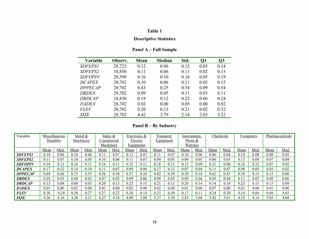
Table 1 provides descriptive statistics for the entire sample (Panel A) and by industry
(Panel B). Recall that we calculate the standard deviation of deflated future earnings per share in
two ways. The first way is based on subsequent reported earnings per share (SDFEPS1). The
second way (SDFEPS2) uses earnings per share adjusted for R&D capitalization. The mean
(median) SDFEPS1 is 0.11 (0.06), quite similar to the distribution of SDFEPS2. The highest
mean and median of SDFEPS1 (0.14 and 0.08, respectively) and of SDFEPS2 (0.13 and 0.08,
respectively) are obtained in the Computers industry. The lowest mean and medians of SDFEPS1
(0.06 and 0.04, respectively) and of SDFEPS2 (0.06 and 0.03, respectively) are obtained in the
Chemicals industry. The range of inter-industry variability of future operating income,
SDFOPIN, is 0.07-0.18 for the mean, and 0.05-0.13 for the median. These facts suggest that the
variability of future performance measures can be quite different across industries. Mean
(median) DRDEX (R&D expenditures over lagged market value of equity) is 0.09 (0.05),
reflecting the focus of this study on R&D-intensive industries. The wide range in the means
13
across industries (0.04-0.11) suggests that the importance of R&D activities may vary
considerably across sample firms. Note that for the entire sample mean DCAPEX (capital
expenditures deflated by lagged market value of equity) is similar to DRDEX. This similarity is
another indicator of the potentially crucial role R&D plays in sample firms. However, PPE tends
to be higher than R&D capital, suggesting that, on average, PPE has longer useful life. Deflated
advertising expense (DADEX) is relatively small, though its mean is quite high for the Chemicals
industry. Leverage (FLEV) seems to be relatively high in the Miscellaneous Durables, Metal and
Machinery, and Transport Equipment. This may be due to greater ability of such industries to
rely on tangible assets as collateral against debt.
(Table 1 about here)
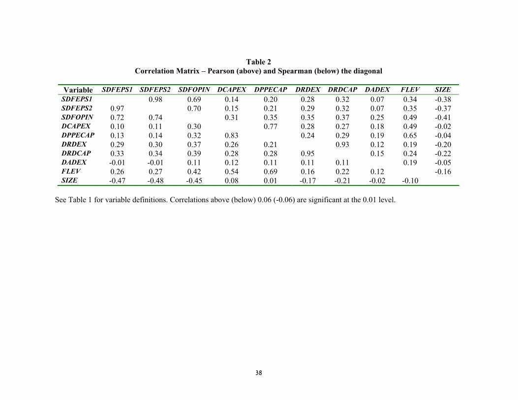
Table 2 provides a correlation matrix for the full sample. Several aspects of this table are
worth noting. First, the Pearson and Spearman correlations between the standard deviation of
future EPS (SDFEPS1) and the standard deviation of future operating income (SDFOPIN) are
0.69 and 0.72, respectively, suggesting that both measures are sufficiently different from each
other to warrant separate analysis. Second, the correlation between R&D expenditures and R&D
capital and between capital expenditure and PPE capital are very high, suggesting that both
measures are expected to yield similar results. Third, SIZE is negatively correlated with the
measures of variability consistent with the argument that larger firms have more stable earnings
and are less risky. Similarly, the positive correlation between leverage (FLEV) and the measures
of variability is consistent with the argument that both leverage and variance of future economic
benefits capture firm risk (Fama and French 1992, 1993). Finally, investments in R&D and fixed
assets are positively correlated with the standard deviation of future economic benefits, although
the degree of correlation differs across the two variability measures.
(Table 2 about here)
14
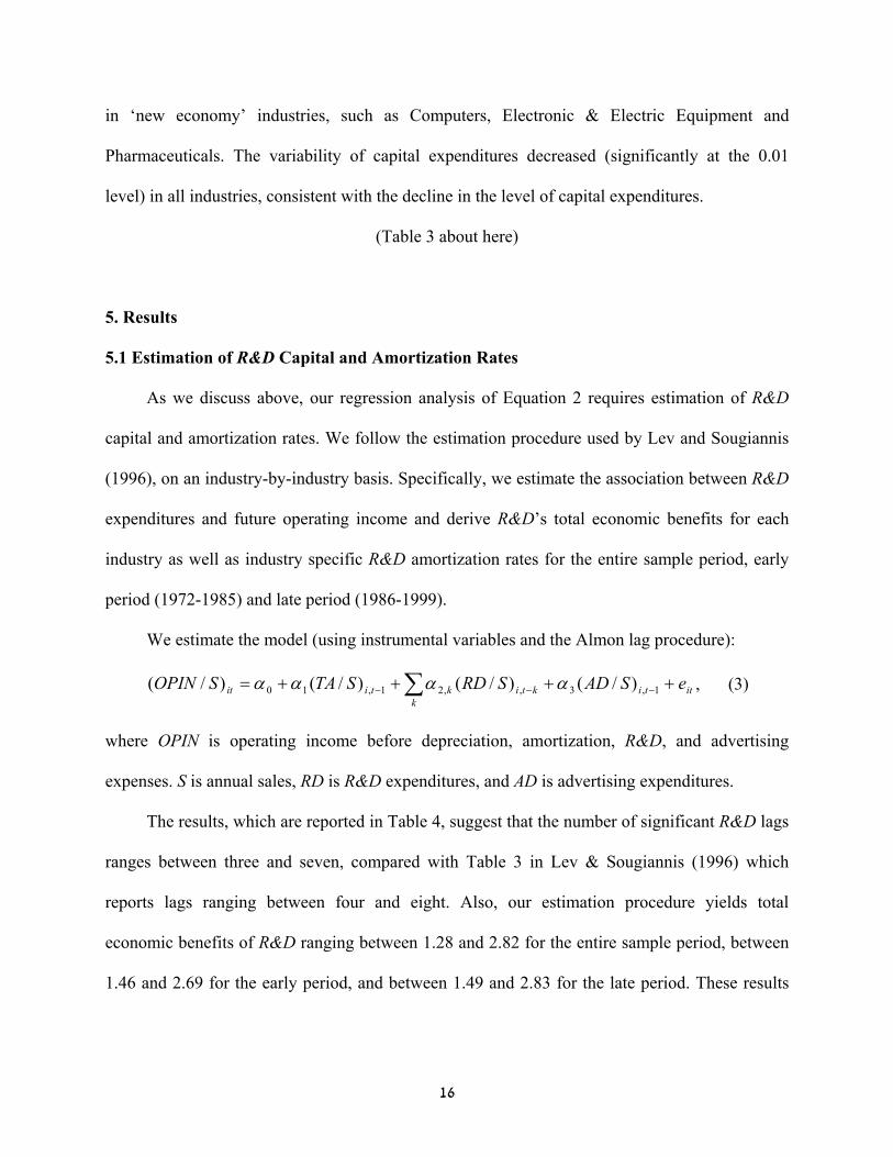
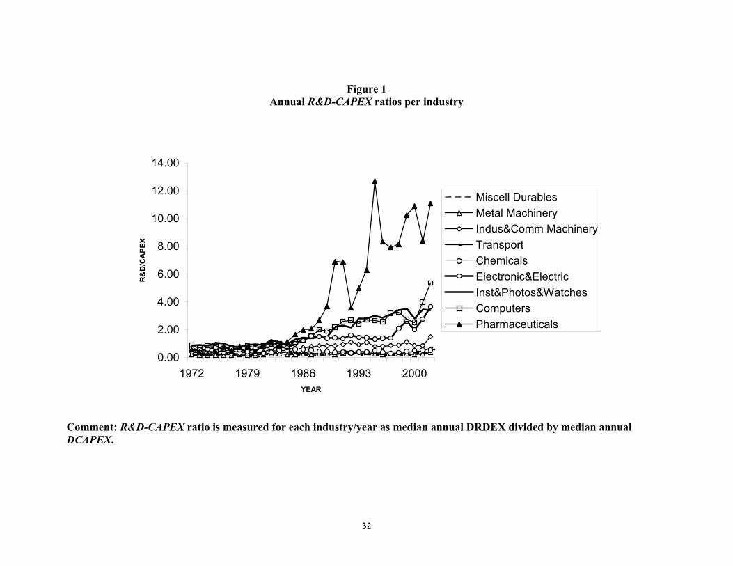
The distribution of R&D and capital intensity has changed over the sample period. Figure 1
presents annual R&D-CAPEX ratios medians of R&D expenditures deflated by annual medians
of capital expenditure for the nine sample industries. Until the mid 1980s all industries exhibit
similar R&D-CAPEX ratio, as can be seen by the tight cluster of industry lines in the early
period. However, after that point in time, this ratio dramatically increases for the Computer,
Measurement Instruments, Photo and Watches, Electronic and other Electric Equipment and
Pharmaceutical industries. Furthermore, this ratio has remained quite similar for the other
industries. In addition, the R&D-CAPEX ratio seems to be quite volatile for the Computer,
Measurement Instruments, Photo and Watches, Electronic and other Electric Equipment and
Pharmaceutical industries, but relatively smooth for the other industries. This pattern suggests a
possible structural change in R&D and innovation strategy in these four highly R&D-intensive
industries. Consequently, we distinguish between two sub-periods: early period (1972-1985) and
late period (1986-1999).3
(Figure 1 about here)
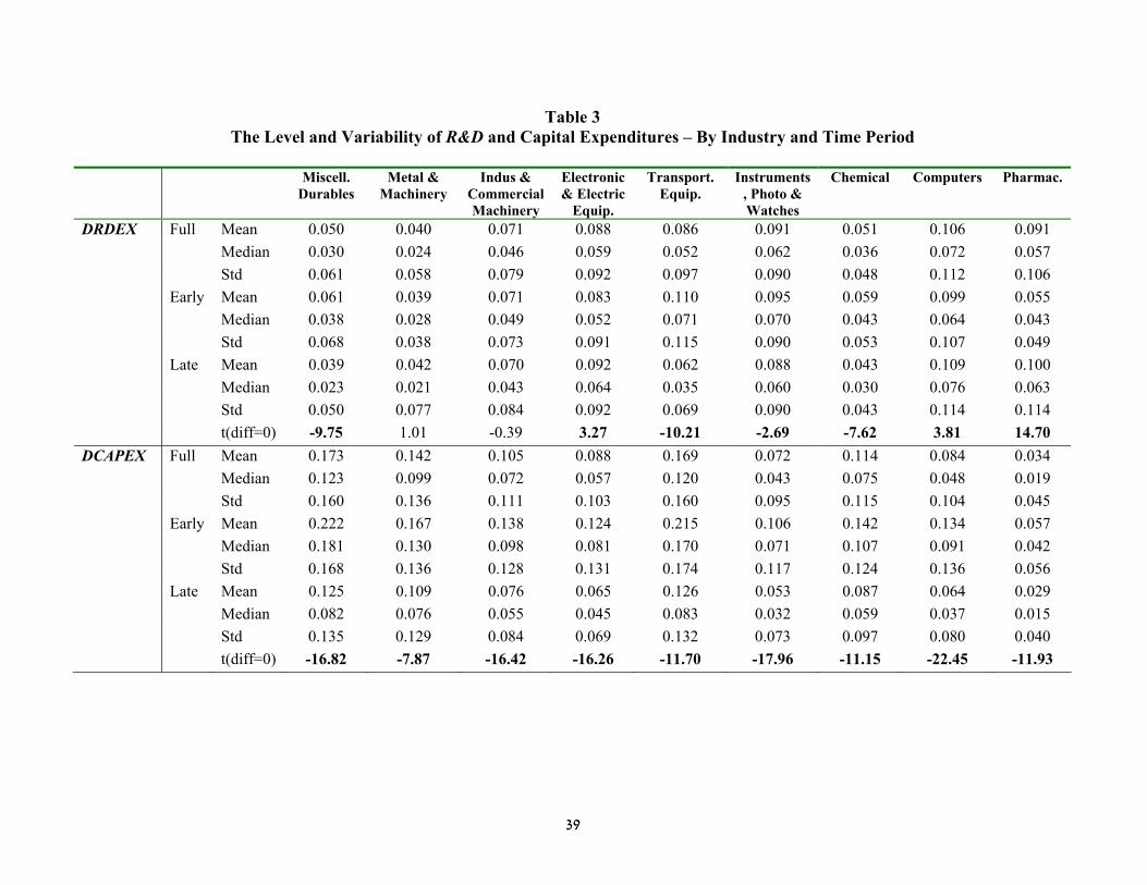
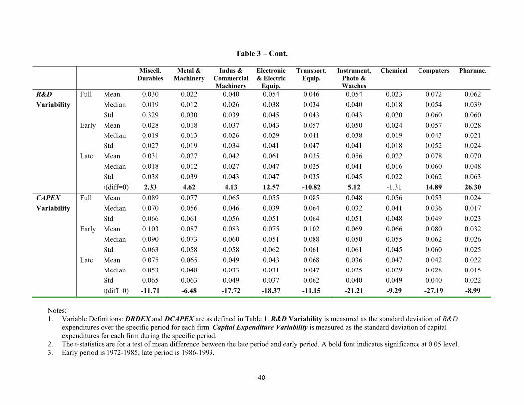
Table 3 provides a formal analysis of the level and variability of R&D and capital
expenditures by industry and time period. Variability is measured as the industry standard
deviation of DRDEX and DCAPEX. We report the t-tests for difference between the early and
late means. Over the entire sample period, the level of R&D expenditure has increased
(significantly at the 0.01 level) in three industries (Computers, Pharmaceuticals and Electronic &
Electric Equipment), decreased (significantly at the 0.01 level) in four industries (Miscellaneous
Durables, Transportation equipment, Instruments Photo & Watches and Chemical), and stayed
=================================================3 This change is associated with a number of developments which took place around that time. For example, Cisco was founded in 1984 and 1986 shipped its first products. The modern Internet came into existence during 1985-1987. IBM devised technology that better links LAN traffic between workstations and servers in 1986 while Sun
15
relatively stable in two industries (Metal & Machinery and Industrial & Commercial Machinery).
Not surprising is the fact that increases in R&D intensity occur in R&D-intensive industries
while decreases in R&D intensity occur in more ‘traditional’ industries. In contrast, the intensity
of capital expenditures has uniformly declined in all industries.
The variability of R&D and capital expenditures also varies across industries and over
time. Potentially owing to scale, the variability of R&D expenditures tends to be higher in R&D-
intensive industries and lower in industries with relatively low R&D intensity. The variability of
R&D increases (significantly at the 0.05 level or better) in seven of the nine industries. R&D
variability is relatively stable in the Chemical industry and has declined in the Transportation
Equipment industry. Note that in the Miscellaneous Durables, and Instruments, Photo &Watches
industries, the variability of R&D expenditures increases over time, though the level of the
expenditures has decreased over time. In the Metal & Machinery and Industrial & Commercial
Machinery industries the variability of R&D expenditures has increased over time, though the
level has been similar. In the Chemicals industry we do not observe any change in the variability,
though the level of R&D expenditure has increased over time. These observations illustrate that
changes over time in the level and variability of R&D need not be of the same sign. That both the
level and variability of R&D have increased most powerfully in the R&D-intensive industries
(e.g., Electronics, Computers and Pharmaceuticals) is consistent with the impact of the
information technology revolution on these industries and is suggestive of larger and more risky
bets taken by firms in the later period than ever before.
Turning to the variability of capital expenditures, note that it is higher in ‘traditional’
industries, such as Rubber & Plastic, Transportation Equipment and Metal Machinery, and lower
==========================================================================================================================================================launched its “The network is the computer” campaign in 1987. In 1990 the World Wide Web was born and the Human Genome project was initiated (and completed in 2003).
16
in ‘new economy’ industries, such as Computers, Electronic & Electric Equipment and
Pharmaceuticals. The variability of capital expenditures decreased (significantly at the 0.01
level) in all industries, consistent with the decline in the level of capital expenditures.
(Table 3 about here)
5. Results
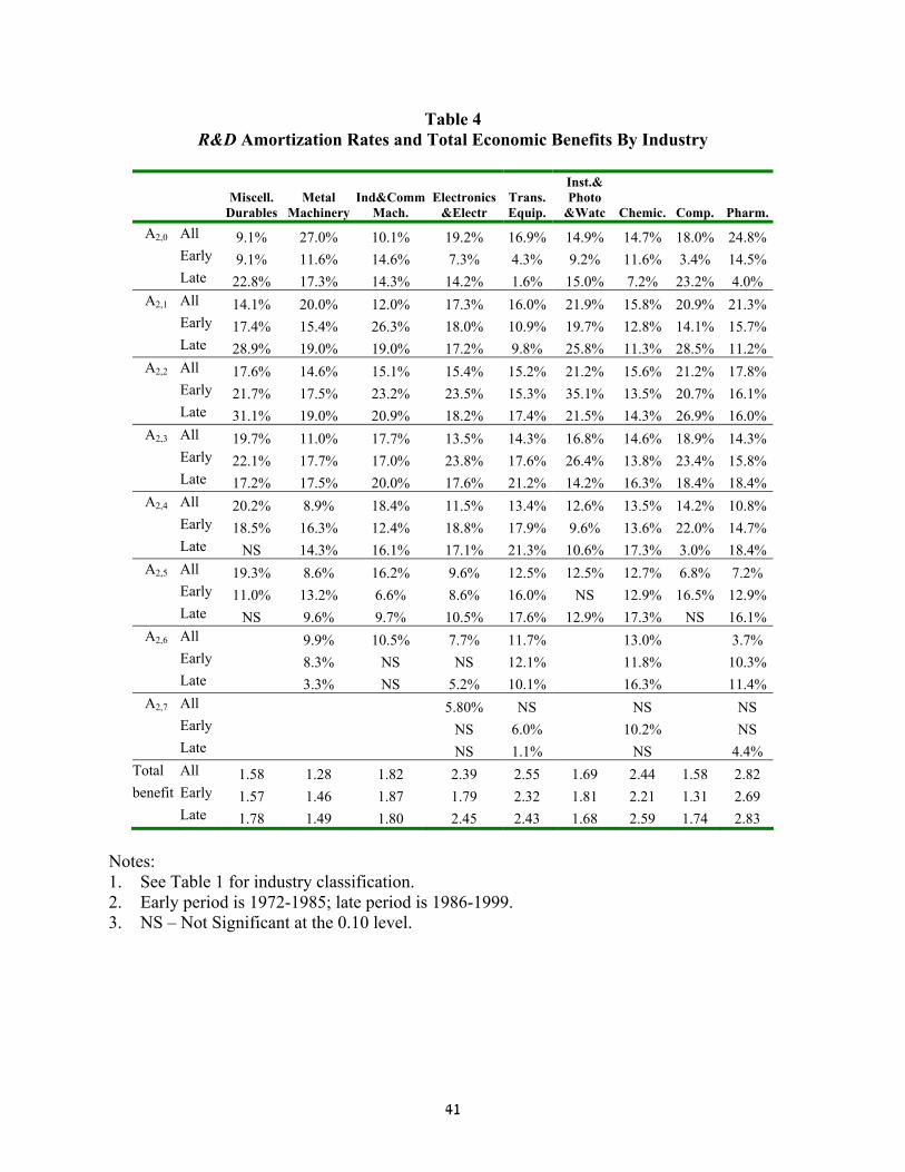
5.1 Estimation of R&D Capital and Amortization Rates
As we discuss above, our regression analysis of Equation 2 requires estimation of R&D
capital and amortization rates. We follow the estimation procedure used by Lev and Sougiannis
(1996), on an industry-by-industry basis. Specifically, we estimate the association between R&D
expenditures and future operating income and derive R&D’s total economic benefits for each
industry as well as industry specific R&D amortization rates for the entire sample period, early
period (1972-1985) and late period (1986-1999).
We estimate the model (using instrumental variables and the Almon lag procedure):
ittiktik
ktiit eSADSRDSTASOPIN ++++= −−− ∑ 1,3,,21,10 )/()/()/()/( αααα , (3)
where OPIN is operating income before depreciation, amortization, R&D, and advertising
expenses. S is annual sales, RD is R&D expenditures, and AD is advertising expenditures.
The results, which are reported in Table 4, suggest that the number of significant R&D lags
ranges between three and seven, compared with Table 3 in Lev & Sougiannis (1996) which
reports lags ranging between four and eight. Also, our estimation procedure yields total
economic benefits of R&D ranging between 1.28 and 2.82 for the entire sample period, between
1.46 and 2.69 for the early period, and between 1.49 and 2.83 for the late period. These results
17
are similar to those reported by Lev and Sougiannis (1996) -- between 1.67 and 2.63 (sample
period up to 1991) -- with chemicals and pharmaceuticals yielding the highest benefits.4
For the entire sample period, total economic return to $1 investment in R&D exceeds 1,
implying that R&D investment is recoverable on average. Total return seems to have increased
over time for all industries except for Industrial & Commercial Machinery and Measurement
Instruments, Photo & Watches. Annual amortization rates vary quite considerably across
industries and time periods. However, for the entire sample period the useful life of R&D capital
is five to seven years.
(Table 4 about here)
5.2 The Association between R&D and Variability of Future Benefits
Before we turn to our industry analysis, we first estimate equations (1) and (2) for the
entire sample using annual cross-sectional regressions and report mean and standard deviation of
the coefficients. All coefficients and t-statistics are adjusted for serial correlation using the
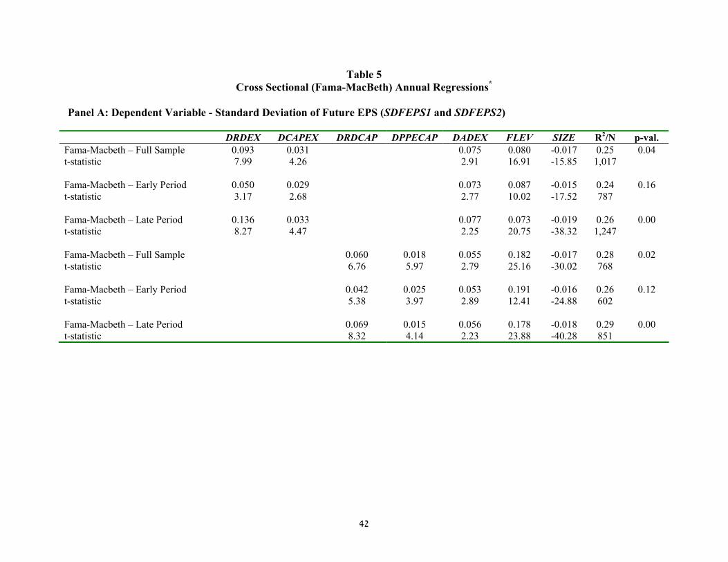
Newey-West (1987) procedure. Panel A of Table 5 presents results for the variability of future
EPS (SDFEPS1 for equation (1) and SDFEPS2 for equation (2)) as a measure of future economic
benefits. At the rightmost column of the panel, we present p-values of the test on the difference
between the coefficients on R&D and capital expenditures.
Estimation results of equation (1) for the entire sample-period yield a positive coefficient
on R&D expenditures (DRDEX). The average coefficient is significantly larger than zero at the
0.01 level. The average coefficient on capital expenditures (DCAPEX) is 0.031, also significantly
different from zero. Also, the average coefficient on DRDEX is larger than the average
coefficient on DCAPEX and the difference is significant at the 0.05 level. These results are
=================================================4 Companies in the Computers industry may choose to capitalize software development costs under SFAS 86.
18
slightly different that those reported by Kothari et al. (2002) as the coefficient on DRDEX in our
study is larger than that reported in their study. There are two possible reasons for these
differences. First, our sample period contains data for 1993-1999, years for which R&D is
presumably more uncertain and earnings are more volatile. Second, our treatment of replacing
missing future earnings is different than the method used by Kothari et al. (2002). Nonetheless,
the main inferences on the differences between the coefficient on R&D and the coefficient on
CAPEX are similar across the two studies.
Similar results are obtained with equation (2), where R&D and fixed capital replace R&D
and capital expenditures, respectively. Specifically, the average coefficient on R&D capital is
positive and significantly different from zero (γ1 = 0.060, t = 6.76); the coefficient on PPE is
significantly different from zero (γ1 = 0.018, t = 5.97). The difference between the two
coefficients is significantly different from zero with a p-value of 0.02.
We also present results for two sub-periods – an early period (1972-1985) and a late period
(1986-1999). Focusing on the late period 1986-1999, the coefficient on R&D expenditures is
0.136 (t = 8.27) whereas the coefficient on capital expenditures is 0.033 (t = 4.47). The
difference between them is significant at the 0.01 level. As for the early period (1972-1985), both
coefficients are positive, but the difference between them is not significantly larger than zero at
the 0.10 level. The results are similar but stronger when R&D capital and PPE are used instead
of R&D expense and capital expenditures, respectively.
To summarize, it is only the later period in which R&D capital contributes more than PPE
to the variability of future EPS. Also, the structural change evidenced in these results relates only
to R&D and not to capital expenditures as the average coefficient on DCAPEX remains relative
constant over time.
19
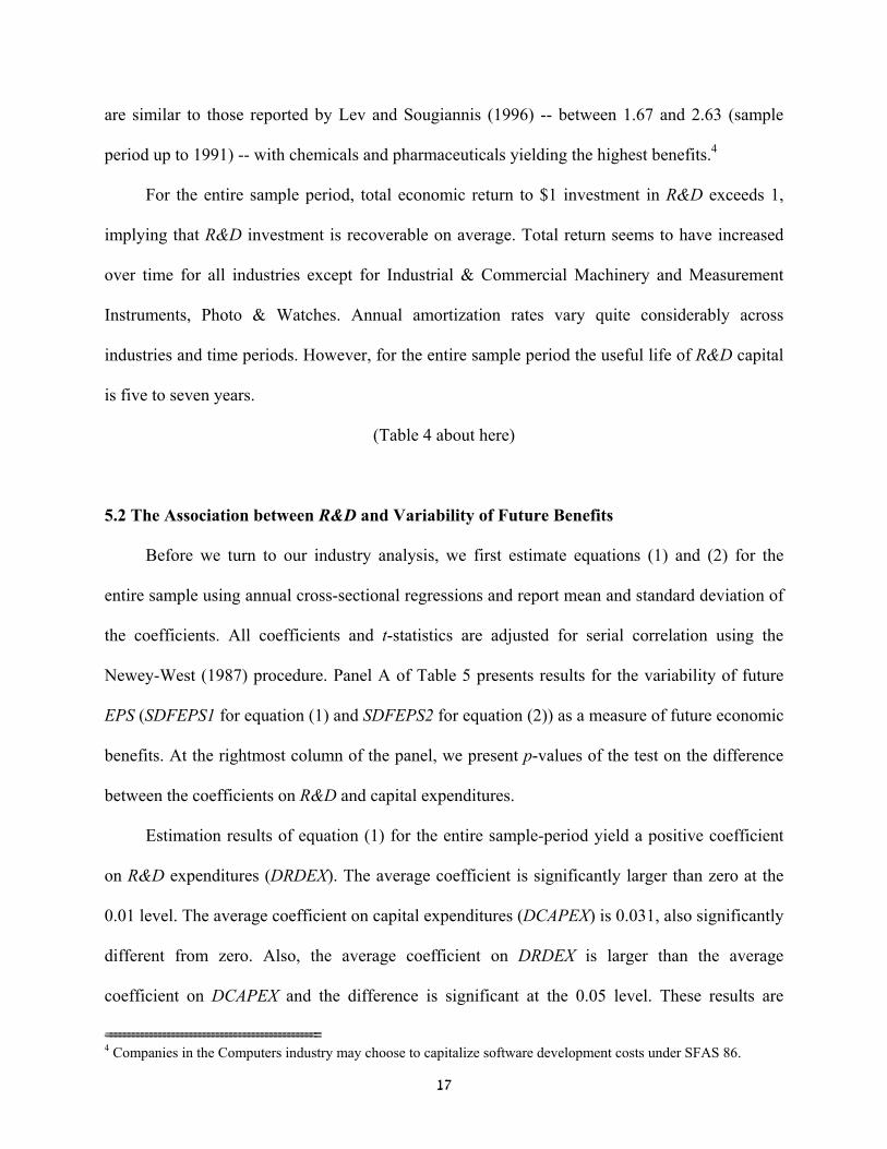
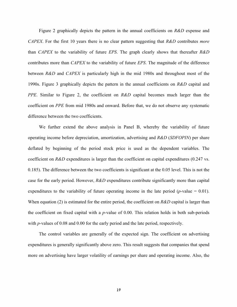
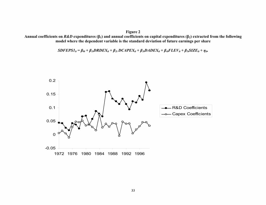
Figure 2 graphically depicts the pattern in the annual coefficients on R&D expense and
CAPEX. For the first 10 years there is no clear pattern suggesting that R&D contributes more
than CAPEX to the variability of future EPS. The graph clearly shows that thereafter R&D
contributes more than CAPEX to the variability of future EPS. The magnitude of the difference
between R&D and CAPEX is particularly high in the mid 1980s and throughout most of the
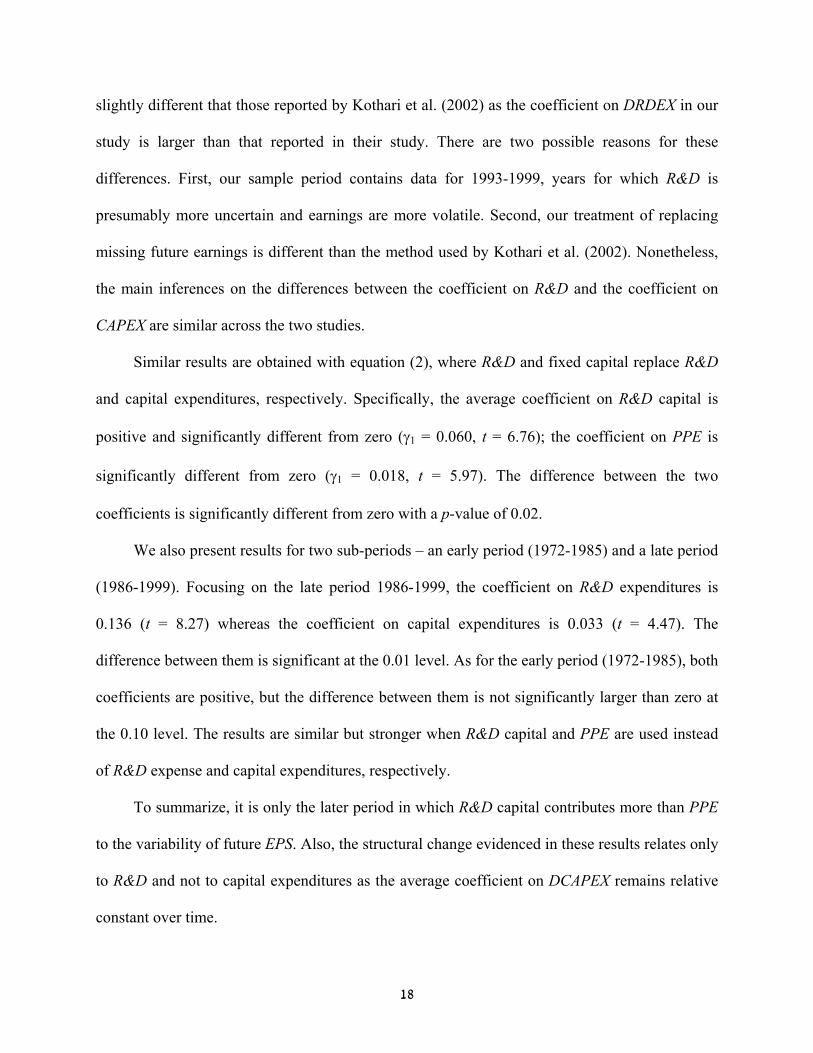
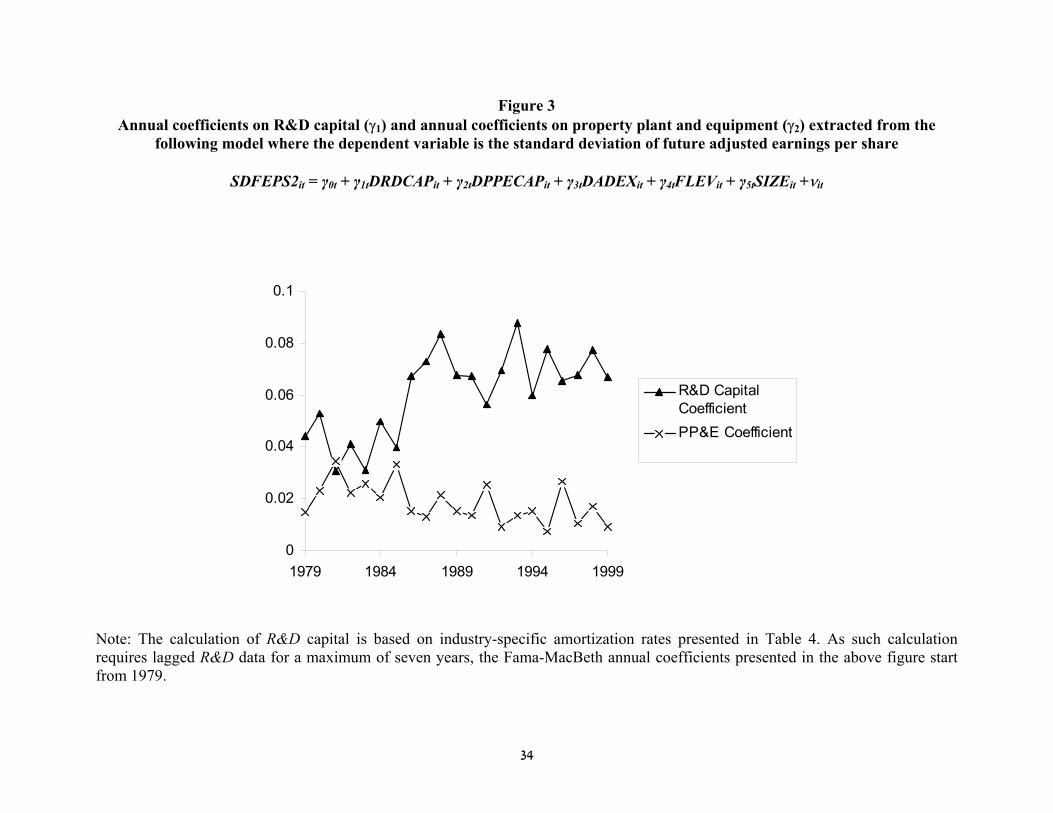
1990s. Figure 3 graphically depicts the pattern in the annual coefficients on R&D capital and
PPE. Similar to Figure 2, the coefficient on R&D capital becomes much larger than the
coefficient on PPE from mid 1980s and onward. Before that, we do not observe any systematic
difference between the two coefficients.
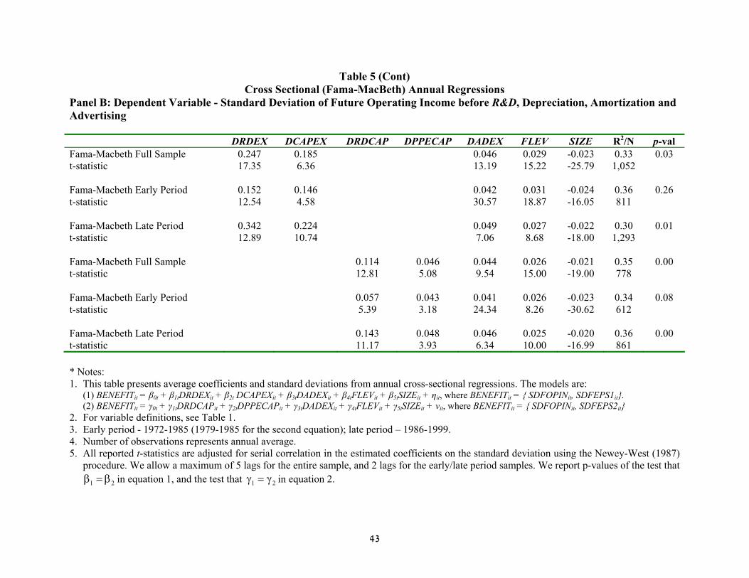
We further extend the above analysis in Panel B, whereby the variability of future
operating income before depreciation, amortization, advertising and R&D (SDFOPIN) per share
deflated by beginning of the period stock price is used as the dependent variables. The
coefficient on R&D expenditures is larger than the coefficient on capital expenditures (0.247 vs.
0.185). The difference between the two coefficients is significant at the 0.05 level. This is not the
case for the early period. However, R&D expenditures contribute significantly more than capital
expenditures to the variability of future operating income in the late period (p-value = 0.01).
When equation (2) is estimated for the entire period, the coefficient on R&D capital is larger than
the coefficient on fixed capital with a p-value of 0.00. This relation holds in both sub-periods
with p-values of 0.08 and 0.00 for the early period and the late period, respectively.
The control variables are generally of the expected sign. The coefficient on advertising
expenditures is generally significantly above zero. This result suggests that companies that spend
more on advertising have larger volatility of earnings per share and operating income. Also, the
20
coefficients on financial leverage are positive and the coefficients on company size are negative,
as expected.
The principal conclusion from this analysis is that R&D contributes more than capital
expenditures to the variability of future EPS and future operating income before R&D,
depreciation and amortization. However, this result is driven primarily by the late sub-period of
1986-1999. Also, the association between R&D and the variability of future economic benefits
has gone through a structural change during the mid-1980. This association has become stronger
while the benchmarked association between capital expenditures and variability of future
economic benefits has remained relatively unchanged.
(Table 5 about here)
5.3 Industry Analysis
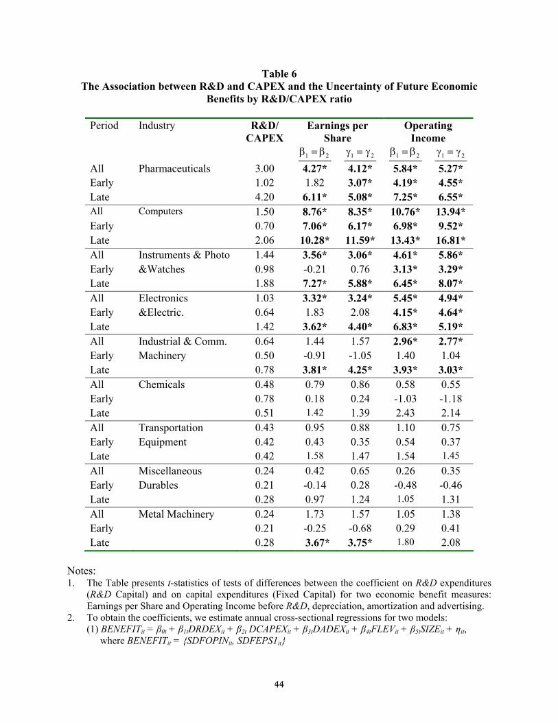
Table 6 reports results for our industry analysis, the prime focus of our study. The table is
organized along three dimensions. First, the nine industries are sorted by descending order of the
R&D-CAPEX ratio. We report the t-statistics for the test that β1, the coefficient on R&D
expenditure, is equal to β2, the coefficient on capital expenditure (Equation 1); and for the test
that γ1, the coefficient on R&D capital, is equal to γ2, the coefficient on PPE capital (Equation 2).
The second dimension relates to measures of future economic benefits. We report results for two
measures: earnings per share and operating income before R&D, depreciation, amortization and
advertising. The third dimension is time. Investment in R&D has become more intense and more
volatile over time due to the effects of the “information revolution.” Also, relative R&D intensity
has increased over time, as shown in Figure 1. In addition, it may have also changed in different
21
directions in different industries as reported in Table 3. To test such effects in the context of our
study, we report results for an early period (1972-1985) and a late period (1986-1999).
To illustrate the structure of the table, consider the t-statistics reported for the
Pharmaceutical industry under the EPS column: When the variability of future EPS is used as a
measure of uncertainty in future economic benefits, the coefficient on R&D capital is larger
(significant at the 0.01 level) than the coefficient on fixed capital, as reflected by the t-statistic of
4.12 under the 1 2γ = γ sub-column. This means that R&D capital contributes more to the
uncertainty in subsequent EPS than PPE. The t-statistic of 4.27 under the 1 2β = β sub-column in
the same industry means that during the late period, the coefficient on R&D expenditures is
larger than the coefficient on capital expenditures, at the 0.01 level. Negative t-statistics suggest
that capital expenditures (or fixed capital) contribute more to the uncertainty of subsequent
economic benefits than R&D expenditures (or R&D capital).5
As table 6 shows, for the entire sample period, in 4 of the 9 industries, the relative intensity
(R&D-CAPEX ratio) is above 1, ranging from 1.03 to 3. This indicates that annual investments in
R&D tend to exceed annual investments in fixed capital, namely, these industries are more R&D-
intensive than capital-intensive. Not surprisingly, these industries – Pharmaceuticals, Computers,
Measurement Instruments & Photo & Watches and Electronics & Electric Equipment – are often
considered as R&D-intensive industries. The other five industries exhibit R&D-CAPEX ratios of
below 1, ranging from 0.24 to 0.64, indicating that these industries are relatively more capital-
intensive. These industries – Industrial & Commercial Machinery, Chemicals, Transportation
Equipment, Miscellaneous Durables and Fabricated Metal & Machinery – are considered as
more ‘traditional’ industries.
22
Consider the four industries that are relatively more R&D-intensive. For the entire sample
period when EPS is used to measure the uncertainty in future economic benefits, the coefficients
on R&D expenditures are larger than those of capital expenditures and significant at the 0.01
level in all four industries. Also, the coefficients on R&D capital are larger than the coefficients
on fixed capital, respectively, in all four industries as reflected by positive and significant t-
statistics.
Now consider the five industries that are relatively more capital-intensive. For the entire
sample period, when EPS is used to measure uncertainty in future economic benefits, R&D
expenditures contribute more than capital expenditures in all five industries as reflected by
positive t-statistics. However, in none of these five industries, the coefficient on R&D
expenditures is larger than that of capital expenditures at the 0.10 level. Similarly, in none of
these five industries, the coefficient on R&D capital is significantly larger than the coefficient on
fixed capital at the 0.05 level. These results suggest that in ‘traditional’ industries R&D
expenditures do not contribute to the uncertainty in future economic benefits significantly more
than capital expenditures. The results for ‘traditional’ industries are generally inconsistent with
the claim that R&D expenditures (R&D capital) have larger effects on the uncertainty of future
economic benefits than capital expenditures (fixed capital).
Generally similar results are obtained when instead of EPS we calculate the volatility of
future benefits using subsequent operating income before R&D, depreciation, amortization and
advertising (SDFOPIN). For the entire sample period, R&D expenses contribute more than
CAPEX in all four R&D-intensive industries and in only one of the five traditional industries.
Similar pattern emerges for R&D capital versus fixed capital for the entire sample period.
==========================================================================================================================================================5 All coefficients and standard deviations are obtained from annual cross sectional regressions (i.e., Fama-MacBeth regressions) and are corrected for serial correlation using the Newey-West (1987) procedure.
23
Consider now the early sample-period 1972-1985. Note that the R&D-CAPEX ratios are
lower than those for the entire sample period. These ratios range from 0.21 for the Metal
Machinery industry to 1.02 in the Pharmaceuticals industry. The contribution of R&D
expenditures and capital expenditures to the uncertainty of future benefits is not identical across
industries and benefit measures. For example, when EPS is used to measure uncertainty in future
benefits, only the Computers industry and Pharmaceuticals industry exhibit positive t-statistics
significant at the 0.01 level for both equations (1) and (2). When operating income is used to
measure uncertainty in future benefits, all the R&D intensive industries exhibit positive t-
statistics significant at the 0.01 level. As another example, consider the Chemicals industry
where for this sub-period capital expenditures and PPE exhibit a stronger impact on EPS
variability than R&D expenditures or R&D capital, as reflected by the negative t-statistics. As for
the relative capital intensive firms, it is observed that generally there is no systematic difference
between R&D and capital expenditures or between R&D capital and PPE.
Turning to the late period 1986-1999, the distribution of R&D-CAPEX across industries
has changed dramatically sharpening the distinction between R&D-intensive and ‘traditional’
industries. In the four R&D-intensive industries the ratios are above one, ranging from 1.42 to
4.2 versus a range of 0.70 to 1.02 in the early period; and in the ‘traditional’ five industries the
ratios are below 1 ranging from 0.28 to 0.78. This range is quite similar to the one in the early
period, suggesting that technological advances have affected ‘traditional’ industries quite
marginally.
Results for the late period suggest that when EPS is used to measure the volatility in future
benefits, the coefficients on R&D expenditures (R&D capital) are larger than the coefficients on
capital expenditures (fixed capital) in all of the four industries that are relatively more R&D-
24
intensive (all 8 t-statistics are positive and significant at the 0.01 level). Turning to the
‘traditional’ industries, only one of the five industries exhibit t-statistics that are positive and
significant at the 0.01 level. Similar results are obtained when operating income is used to
measure uncertainty in future benefits.
Overall, the results in Table 6 suggest that the effect of R&D activities on the uncertainty
of future economic benefits is stronger than that of capital expenditures primarily in industries
that are relatively R&D-intensive, as measured by the R&D-CAPEX ratio. Furthermore, this
result is driven by recent years as R&D investments have potentially become more uncertain.
This result does not generally hold in industries that are relatively capital-intensive.
(Table 6 about here)
5.4 Frequency Analysis
The discussion thus far has focused on the effect of R&D on uncertainty of future
economic benefits. However, this discussion has ignored an important feature of accounting
recognition: the likelihood of recoverability. A cost could be associated with uncertain future
benefits but the likelihood of recoverability could still be very high. Table 4 shows that
investment in R&D is recoverable on average. But it is silent on the probability that such
investment will generate returns higher than the initial investment. To examine the likelihood of
recoverability, we measure the frequency of increases (decreases) in future earnings per share
following increases (decreases) in R&D and capital expenditures. Table 7 reports the results for
the nine industries, over five periods subsequent to changes in R&D and capital expenditures.
For brevity, we report the results for only earnings per share for the entire sample-period.
25
Consider first the frequencies associated with R&D expenditures. For industries that are
relatively more R&D-intensive these frequencies are 54.65%, 53.46%, 53.08%, 52.44% and
51.32% for one through five periods ahead, respectively. These frequencies are lower (at the 0.05
level) than the corresponding frequencies for industries that are relatively capital-intensive
(59.17%, 57.01%, 56.06%, 56.00%, and 54.28%). Next consider the frequencies associated with
capital expenditures. These frequencies are similar across the two industry types.
The variable of importance is the difference between the frequencies associated with R&D
expenditures with the corresponding frequencies associated with capital expenditures. For
industries that are relatively more R&D-intensive these differences are -4.71%, -3.78%, -3.64%,
-3.50% and -3.26% for the subsequent five periods, respectively, suggesting that the probability
of recoverability is lower for R&D expenditures than for capital expenditures. For industries that
are relatively more capital-intensive, these differences are -1.97%, 0.22%, 0.02%, 0.15% and -
0.02%, respectively, suggesting that R&D expenditures may not be less recoverable than capital
expenditures in these industries. Furthermore, the differences in frequencies between R&D and
capital expenditures in R&D intensive industries are all significant at the 0.01 level using a t-test
(t-statistics, which are not reported in a table, are -13.2, -27.8, -27.4, -26.7, and -25.5 for the five
subsequent periods, respectively).
The results in Table 7 highlight an important difference between the two types of
industries: On average, R&D expenditures are less certain and less likely to be recovered than
capital expenditures. However, this is driven by R&D-intensive industries for which R&D is
expected to involve higher risk. In industries that are relatively less R&D-dependent, R&D
expenditures are as likely as capital expenditures to be recovered.
(Table 7 about here)
26
5.5 Additional Analysis – The Effect of Variability in R&D Expense and CAPEX
The relative effect of R&D and capital expenditures on future performance uncertainty
may be influenced by their respective volatility. It is possible that the variability of past and
current expenditures is an important determinant of future uncertainty and that it is also
correlated with level of these expenditures. To control for this potentially omitted correlated
variable problem, we calculate the standard deviation of R&D (SDRDEX) and capital
expenditures (SDCAPEX) for each firm over a five-year period that ends in year t-1.
To examine the effect of volatility in R&D and CAPEX on the previous findings, we re-
estimate equations (1) and (2) after controlling for the volatility of R&D and capital
expenditures:
BENEFITit = β0t + β1tDRDEXit + β2tDCAPEXit + β3tDADEXit + β4tFLEVit + β5tSIZEit +
β6tSDRDEXit-1 + β7tSDCAPEXit-1 + ηit (1a)
where BENEFITit = {SDFOPINit, SDFEPS1it}.
BENEFITit = γ0t + γ1tDRDCAPit + γ2tDPPECAPit + γ3tDADEXit + γ4tFLEVit + γ5tSIZEit +
γ6tSDRDEXit-1 + γ7tSDCAPEXit-1 + ηit, (2a)
where BENEFITit = {SDFOPINit, SDFEPS2it}.
We conduct the following tests, expressed as two hypotheses in their null form:
(i) The coefficient on R&D expenditures, DRDEX, is equal to the coefficient on capital
expenditures, DCAPEX. That is: β1 = β2.
27
(ii) The coefficient on R&D volatility, SDRDEX, is equal to the coefficient on CAPEX
volatility, SDCAPEX, That is: β6 = β7.6
The evidence, which is not tabulated here, suggests that including volatility measures in
equations (1) and (2) does not change our prior inferences in a fundamental way. That is, the
results reported on Table 6 are largely unaffected by the inclusion of volatility measures, as
reflected by the results of the first test, β1 = β2. As in Table 6, the coefficients on R&D
expenditures are larger than the coefficients on capital expenditures for relatively R&D-intensive
industries but not for relatively capital-intensive ones. However, with uncertainty of EPS being
the dependent variable, inclusion of the volatility variables weakens the significance of the t-
statistics for the traditional industries in the late period, providing further support to the
observation that the impact of R&D on future EPS uncertainty is driven by R&D-intensive firms
in recent years.
The second result is that the volatility of R&D is more strongly related to the variability of
future EPS than the volatility of capital expenditures in 6 of the 9 industries. This is reflected by
the positive and significant t-statistic in our second test, β6 = β7. This result, which is driven by
the late period, suggests that more volatile R&D expenditures are associated with more volatile
future EPS.
To summarize, inclusion of the volatility variables does not alter the main inference
regarding the relative effect of R&D intensity vs. capital expense on uncertainty of future
performance. Nonetheless, the volatility of R&D and capital expenditures do influence future
performance uncertainty.
=================================================6 As before, all coefficients and standard deviations are obtained from annual cross sectional regressions.
28
6. Summary and Conclusions
One important aspect of asset recognition relates to the association between an expenditure
and future economic benefits. While much of the research on accounting for R&D has focused
on the value-relevance of R&D outlays, the uncertainty of R&D expenditures has received little
attention. An exception is Kothari et al. (2002) who examine the association between current
R&D and capital expenditures and the variability of subsequent earnings per share. They argue
that, on average, R&D is significantly more strongly associated with subsequent earnings per
share than capital expenditures. This result has implications for standard setting; in particular, it
supports the current treatment of full expensing of R&D expenditures under US GAAP.
However, if one is willing to relax the presumption of uniform accounting across different
industries, then a large sample study that spans a very large number of industries may obscure
the true nature of the association between R&D and volatility of future economic benefits. We
therefore study the issue in an industry context and show that the relation between R&D and the
volatility of future economic benefits varies over time and by industry in a predictable manner.
In particular, our study shows that R&D contributes more than capital expenditures to the
volatility of future economic benefits in industries in which R&D is relatively more intensive
than capital but not in industries in which capital is relatively more intensive than R&D.
Specifically, to conduct a meaningful industry analysis we limit our study to nine
industries with sufficiently high number of observations. For each industry we calculate a
relative intensity measure – R&D expenditures divided by capital expenditures (R&D-CAPEX
ratio). Then we show that R&D contributes more than capital expenditures to the variability in
future earnings per share only in industries that are relatively more R&D intensive but not in
industries that are relatively more capital intensive. In addition, we show that R&D has become
more uncertain over time. Finally, we conduct a frequency test aimed at measuring the likelihood
29
of recoverability of R&D and capital expenditures. We find that R&D expenditures are less
likely to be recovered only in industries that are relatively R&D-intensive.
Our results have some interesting implications for standard setting and financial statement
analysis. First, the results suggest that a uniform accounting rule (either expensing or
capitalization) for R&D expenditures may not be justified under classic accounting theory. Our
results support an accounting rule that takes into account industry and firm specific
circumstances, such as SFAS 86 (computer software development costs) and International
Accounting Standard (IAS) 38, Intangible Assets, whereby development costs are expensed or
capitalized depending on firm and market specific circumstances.
30
References
Accounting Principles Board, 1970, APB Statement Number 4. New York, New York. Amir, E., B. Lev, and T. Sougiannis, 2003, “Do Financial Analysts Get Intangibles?” European Accounting Review 12 (4):635-661. Chan, S., J. Martin, and J. Kensinger, 1990, “Corporate research and development expenditures and share value.” Journal of Financial Economics 26, 255-276. Dukes, R.E., T.R. Dyckman, and J.A. Elliott, 1980, “Accounting for research and development costs: The impact on research and development expenditures.” Journal of Accounting Research 18 (Supplement), 1-26. Fama, E., and K. French, 1992, “The cross-section of expected returns.” Journal of Finance 47, 427-465. Fama, E.F., and K.R. French, 1993, “Common risk factors in the returns of stocks and bonds.” Journal of Financial Economics 33: 3-56. Fama, E., and J. Macbeth, 1973, “Risk, return, and equilibrium: Empirical tests.” Journal of Political Economy 81, 607-636. Financial Accounting Standard Board, 1974. Statement of Financial Accounting Standard No. 2: Accounting For Research and Development. Stamford, Conn: FASB. Financial Accounting Standard Board, 1980a, Statement of Financial Accounting Concept No. 2: Qualitative Characteristics of Accounting Information. Stamford, CN: FASB. Financial Accounting Standard Board, 1980b, Statement of Financial Accounting Concept No. 6: Elements of Financial Statements. Stamford, CN: FASB. Financial Accounting Standard Board, 1985, Statement of Financial Accounting Standard No. 86: Accounting For Software Development Costs. Stamford, CN: FASB. Healy, P.M., S.C. Myers, and C.D. Howe, 2002, “R&D accounting and the tradeoff between relevance and objectivity.” Journal of Accounting Research 40 (3): 677-710. Hirschey, M., and J. Weygandt, 1985, “Amortization policy for advertising and research and development expenditures.” Journal of Accounting Research 23: 326-385. International Accounting Standards Board, 2004, International Accounting Standard No. 38: Intangible Assets (Revised): London, IASB.
31
Kothari, S.P., T.E. Laguerre, and A.J Leone, 2002, “Capitalization versus expensing: Evidence on the uncertainty of future earnings from capital expenditures versus R&D outlays.” Review of Accounting Studies 7 (4): 355-382. Lev, B. and T. Sougiannis, 1996, “The capitalization, amortization, and value-relevance of R&D.” Journal of Accounting Economics 21: 107-138. Newey, W.K., and K.D. West, 1987, “A simple, positive semi-definite heteroscedasticity and autocorrelation consistent covariance matrix.” Econometrica 55, 703-708. Newey, W.K., and K.D. West, 1994, “Automatic lag selection in covariance matrix estimation.” Review of Economic Studies 61, 631-653. Shi, C., 2003, “On the trade-off between the future benefits and the riskiness of R&D: a bondholders’ perspective.” Journal of Accounting and Economics 35: 227-254. Sougiannis, T., 1994, “The accounting based valuation of corporate R&D.” The Accounting Review 69, 44-68. Wasley, C.E., and T.J. Linsmeier, 1992, “A further examination of the economic consequences of SFAS No. 2.” Journal of Accounting Research 30, 156-164.
32
Figure 1 Annual R&D-CAPEX ratios per industry
0.00
2.00
4.00
6.00
8.00
10.00
12.00
14.00
1972 1979 1986 1993 2000YEAR
R&
D/C
APE
X
Miscell DurablesMetal MachineryIndus&Comm MachineryTransportChemicalsElectronic&ElectricInst&Photos&WatchesComputersPharmaceuticals
Comment: R&D-CAPEX ratio is measured for each industry/year as median annual DRDEX divided by median annual DCAPEX.
33
Figure 2 Annual coefficients on R&D expenditures (β1) and annual coefficients on capital expenditures (β2) extracted from the following
model where the dependent variable is the standard deviation of future earnings per share
SDFEPS1it = β0t + β1tDRDEXit + β2t DCAPEXit + β3tDADEXit + β4tFLEVit + β5tSIZEit + ηit.
-0.05
0
0.05
0.1
0.15
0.2
1972 1976 1980 1984 1988 1992 1996
R&D CoefficientsCapex Coefficients
34
Figure 3 Annual coefficients on R&D capital (γ1) and annual coefficients on property plant and equipment (γ2) extracted from the
following model where the dependent variable is the standard deviation of future adjusted earnings per share
SDFEPS2it = γ0t + γ1tDRDCAPit + γ2tDPPECAPit + γ3tDADEXit + γ4tFLEVit + γ5tSIZEit +νit
0
0.02
0.04
0.06
0.08
0.1
1979 1984 1989 1994 1999
R&D CapitalCoefficientPP&E Coefficient
Note: The calculation of R&D capital is based on industry-specific amortization rates presented in Table 4. As such calculation requires lagged R&D data for a maximum of seven years, the Fama-MacBeth annual coefficients presented in the above figure start from 1979.
35
Table 1
Descriptive Statistics
Panel A – Full Sample
Variable Observ. Mean Median Std. Q1 Q3 SDFEPS1 28,722 0.12 0.06 0.12 0.03 0.14 SDFEPS2 18,850 0.11 0.06 0.11 0.02 0.13 SDFOPIN 28,599 0.16 0.10 0.16 0.05 0.19 DCAPEX 28,702 0.10 0.06 0.11 0.02 0.12 DPPECAP 28,702 0.43 0.25 0.54 0.09 0.54 DRDEX 28,702 0.09 0.05 0.11 0.03 0.11 DRDCAP 18,850 0.19 0.12 0.22 0.06 0.24 DADEX 28,702 0.02 0.00 0.05 0.00 0.02 FLEV 28,702 0.20 0.13 0.21 0.02 0.32 SIZE 28,702 4.42 3.79 2.14 2.85 5.22
Panel B – By Industry
Variable Miscellaneous
Durables Metal &
Machinery Indus &
Commercial Machinery
Electronic & Electric
Equipment
Transport. Equipment
Instruments, Photo & Watches
Chemicals Computers Pharmaceuticals
Mean Med. Mean Med. Mean Med. Mean Med. Mean Med. Mean Med. Mean Med. Mean Med. Mean Med. SDFEPS1 0.10 0.06 0.10 0.06 0.11 0.07 0.11 0.07 0.11 0.07 0.10 0.06 0.06 0.04 0.14 0.08 0.08 0.05 SDFEPS2 0.11 0.07 0.10 0.05 0.10 0.06 0.11 0.07 0.09 0.05 0.09 0.05 0.06 0.03 0.13 0.08 0.07 0.04 SDFOPIN 0.18 0.13 0.16 0.11 0.16 0.11 0.15 0.11 0.18 0.13 0.13 0.09 0.11 0.08 0.16 0.12 0.07 0.05 DCAPEX 0.17 0.12 0.14 0.10 0.11 0.07 0.09 0.06 0.17 0.12 0.07 0.04 0.11 0.07 0.08 0.05 0.03 0.02 DPPECAP 0.89 0.60 0.75 0.55 0.56 0.38 0.37 0.24 0.82 0.59 0.30 0.18 0.62 0.43 0.28 0.15 0.15 0.08 DRDEX 0.05 0.03 0.04 0.02 0.07 0.05 0.09 0.06 0.09 0.05 0.09 0.06 0.05 0.04 0.11 0.07 0.09 0.06 DRDCAP 0.13 0.09 0.08 0.05 0.20 0.13 0.23 0.15 0.21 0.13 0.20 0.14 0.14 0.10 0.23 0.15 0.15 0.09 DADEX 0.03 0.00 0.02 0.00 0.02 0.00 0.02 0.00 0.02 0.00 0.01 0.00 0.07 0.00 0.01 0.00 0.01 0.00 FLEV 0.30 0.24 0.30 0.27 0.27 0.22 0.20 0.14 0.33 0.30 0.17 0.11 0.24 0.20 0.14 0.06 0.08 0.03 SIZE 4.26 4.10 4.26 4.11 4.27 4.18 4.09 3.88 5.37 5.50 3.83 3.60 5.42 5.61 4.35 4.14 5.05 4.68
36
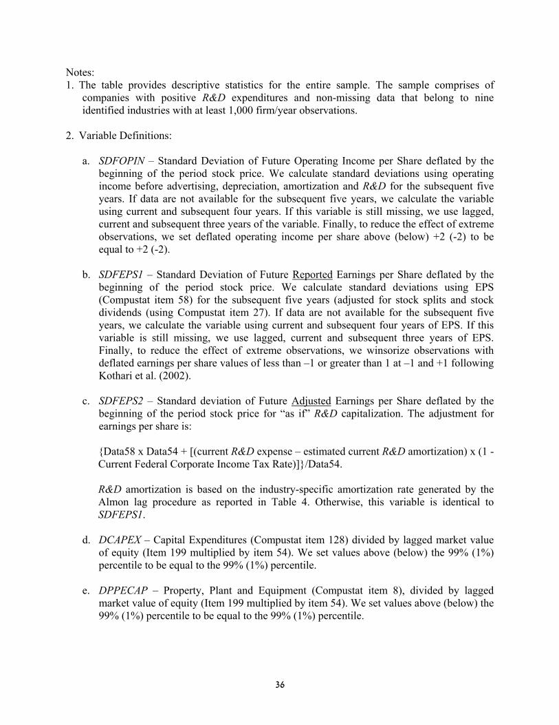
Notes: 1. The table provides descriptive statistics for the entire sample. The sample comprises of
companies with positive R&D expenditures and non-missing data that belong to nine identified industries with at least 1,000 firm/year observations.
2. Variable Definitions:
a. SDFOPIN – Standard Deviation of Future Operating Income per Share deflated by the beginning of the period stock price. We calculate standard deviations using operating income before advertising, depreciation, amortization and R&D for the subsequent five years. If data are not available for the subsequent five years, we calculate the variable using current and subsequent four years. If this variable is still missing, we use lagged, current and subsequent three years of the variable. Finally, to reduce the effect of extreme observations, we set deflated operating income per share above (below) +2 (-2) to be equal to +2 (-2).
b. SDFEPS1 – Standard Deviation of Future Reported Earnings per Share deflated by the
beginning of the period stock price. We calculate standard deviations using EPS (Compustat item 58) for the subsequent five years (adjusted for stock splits and stock dividends (using Compustat item 27). If data are not available for the subsequent five years, we calculate the variable using current and subsequent four years of EPS. If this variable is still missing, we use lagged, current and subsequent three years of EPS. Finally, to reduce the effect of extreme observations, we winsorize observations with deflated earnings per share values of less than –1 or greater than 1 at –1 and +1 following Kothari et al. (2002).
c. SDFEPS2 – Standard deviation of Future Adjusted Earnings per Share deflated by the
beginning of the period stock price for “as if” R&D capitalization. The adjustment for earnings per share is:
{Data58 x Data54 + [(current R&D expense – estimated current R&D amortization) x (1 - Current Federal Corporate Income Tax Rate)]}/Data54. R&D amortization is based on the industry-specific amortization rate generated by the Almon lag procedure as reported in Table 4. Otherwise, this variable is identical to SDFEPS1.
d. DCAPEX – Capital Expenditures (Compustat item 128) divided by lagged market value
of equity (Item 199 multiplied by item 54). We set values above (below) the 99% (1%) percentile to be equal to the 99% (1%) percentile.
e. DPPECAP – Property, Plant and Equipment (Compustat item 8), divided by lagged
market value of equity (Item 199 multiplied by item 54). We set values above (below) the 99% (1%) percentile to be equal to the 99% (1%) percentile.
37
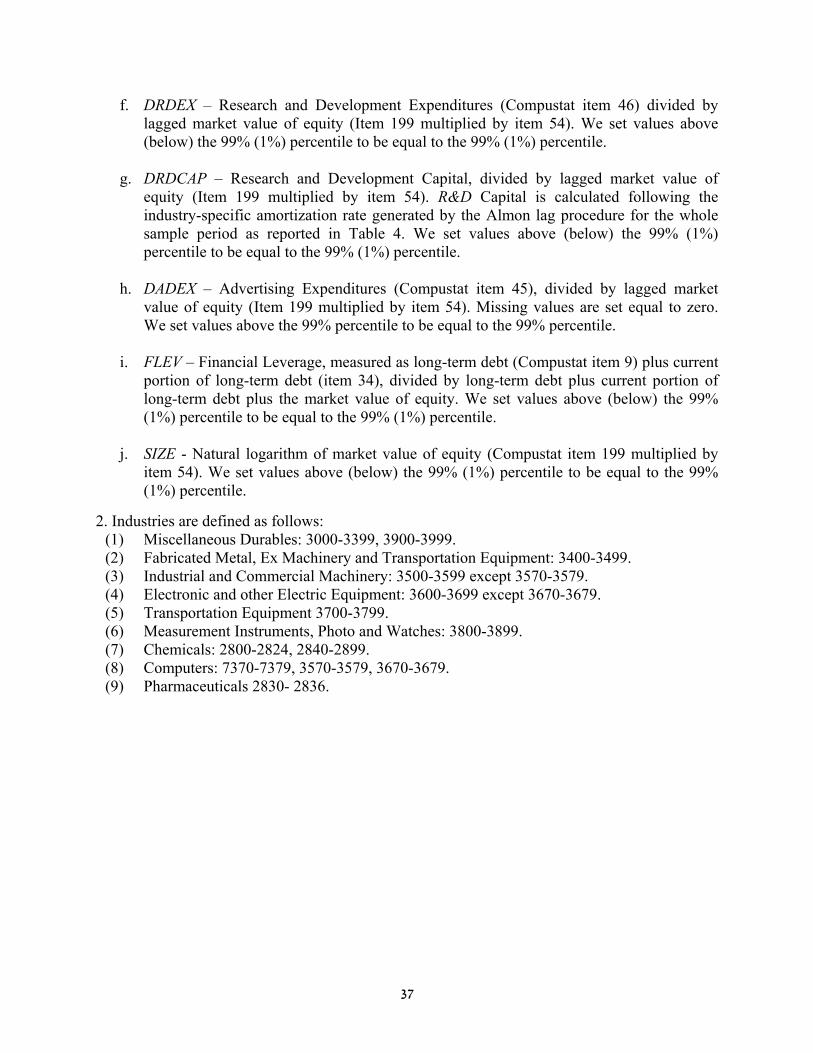
f. DRDEX – Research and Development Expenditures (Compustat item 46) divided by lagged market value of equity (Item 199 multiplied by item 54). We set values above (below) the 99% (1%) percentile to be equal to the 99% (1%) percentile.
g. DRDCAP – Research and Development Capital, divided by lagged market value of
equity (Item 199 multiplied by item 54). R&D Capital is calculated following the industry-specific amortization rate generated by the Almon lag procedure for the whole sample period as reported in Table 4. We set values above (below) the 99% (1%) percentile to be equal to the 99% (1%) percentile.
h. DADEX – Advertising Expenditures (Compustat item 45), divided by lagged market
value of equity (Item 199 multiplied by item 54). Missing values are set equal to zero. We set values above the 99% percentile to be equal to the 99% percentile.
i. FLEV – Financial Leverage, measured as long-term debt (Compustat item 9) plus current
portion of long-term debt (item 34), divided by long-term debt plus current portion of long-term debt plus the market value of equity. We set values above (below) the 99% (1%) percentile to be equal to the 99% (1%) percentile.
j. SIZE - Natural logarithm of market value of equity (Compustat item 199 multiplied by
item 54). We set values above (below) the 99% (1%) percentile to be equal to the 99% (1%) percentile.
2. Industries are defined as follows:
(1) Miscellaneous Durables: 3000-3399, 3900-3999. (2) Fabricated Metal, Ex Machinery and Transportation Equipment: 3400-3499. (3) Industrial and Commercial Machinery: 3500-3599 except 3570-3579. (4) Electronic and other Electric Equipment: 3600-3699 except 3670-3679. (5) Transportation Equipment 3700-3799. (6) Measurement Instruments, Photo and Watches: 3800-3899. (7) Chemicals: 2800-2824, 2840-2899. (8) Computers: 7370-7379, 3570-3579, 3670-3679. (9) Pharmaceuticals 2830- 2836.
38
Table 2
Correlation Matrix – Pearson (above) and Spearman (below) the diagonal
Variable SDFEPS1 SDFEPS2 SDFOPIN DCAPEX DPPECAP DRDEX DRDCAP DADEX FLEV SIZE
SDFEPS1 0.98 0.69 0.14 0.20 0.28 0.32 0.07 0.34 -0.38 SDFEPS2 0.97 0.70 0.15 0.21 0.29 0.32 0.07 0.35 -0.37 SDFOPIN 0.72 0.74 0.31 0.35 0.35 0.37 0.25 0.49 -0.41 DCAPEX 0.10 0.11 0.30 0.77 0.28 0.27 0.18 0.49 -0.02 DPPECAP 0.13 0.14 0.32 0.83 0.24 0.29 0.19 0.65 -0.04 DRDEX 0.29 0.30 0.37 0.26 0.21 0.93 0.12 0.19 -0.20 DRDCAP 0.33 0.34 0.39 0.28 0.28 0.95 0.15 0.24 -0.22 DADEX -0.01 -0.01 0.11 0.12 0.11 0.11 0.11 0.19 -0.05 FLEV 0.26 0.27 0.42 0.54 0.69 0.16 0.22 0.12 -0.16 SIZE -0.47 -0.48 -0.45 0.08 0.01 -0.17 -0.21 -0.02 -0.10
See Table 1 for variable definitions. Correlations above (below) 0.06 (-0.06) are significant at the 0.01 level.
39
Table 3 The Level and Variability of R&D and Capital Expenditures – By Industry and Time Period
Miscell.
Durables Metal &
Machinery Indus &
Commercial Machinery
Electronic & Electric
Equip.
Transport. Equip.
Instruments, Photo & Watches
Chemical Computers Pharmac.
DRDEX Full Mean 0.050 0.040 0.071 0.088 0.086 0.091 0.051 0.106 0.091 Median 0.030 0.024 0.046 0.059 0.052 0.062 0.036 0.072 0.057 Std 0.061 0.058 0.079 0.092 0.097 0.090 0.048 0.112 0.106 Early Mean 0.061 0.039 0.071 0.083 0.110 0.095 0.059 0.099 0.055 Median 0.038 0.028 0.049 0.052 0.071 0.070 0.043 0.064 0.043 Std 0.068 0.038 0.073 0.091 0.115 0.090 0.053 0.107 0.049 Late Mean 0.039 0.042 0.070 0.092 0.062 0.088 0.043 0.109 0.100 Median 0.023 0.021 0.043 0.064 0.035 0.060 0.030 0.076 0.063 Std 0.050 0.077 0.084 0.092 0.069 0.090 0.043 0.114 0.114 t(diff=0) -9.75 1.01 -0.39 3.27 -10.21 -2.69 -7.62 3.81 14.70 DCAPEX Full Mean 0.173 0.142 0.105 0.088 0.169 0.072 0.114 0.084 0.034 Median 0.123 0.099 0.072 0.057 0.120 0.043 0.075 0.048 0.019 Std 0.160 0.136 0.111 0.103 0.160 0.095 0.115 0.104 0.045 Early Mean 0.222 0.167 0.138 0.124 0.215 0.106 0.142 0.134 0.057 Median 0.181 0.130 0.098 0.081 0.170 0.071 0.107 0.091 0.042 Std 0.168 0.136 0.128 0.131 0.174 0.117 0.124 0.136 0.056 Late Mean 0.125 0.109 0.076 0.065 0.126 0.053 0.087 0.064 0.029 Median 0.082 0.076 0.055 0.045 0.083 0.032 0.059 0.037 0.015 Std 0.135 0.129 0.084 0.069 0.132 0.073 0.097 0.080 0.040 t(diff=0) -16.82 -7.87 -16.42 -16.26 -11.70 -17.96 -11.15 -22.45 -11.93
40
Table 3 – Cont.
Miscell. Durables
Metal & Machinery
Indus & Commercial Machinery
Electronic & Electric
Equip.
Transport. Equip.
Instrument, Photo & Watches
Chemical Computers Pharmac.
R&D Full Mean 0.030 0.022 0.040 0.054 0.046 0.054 0.023 0.072 0.062 Variability Median 0.019 0.012 0.026 0.038 0.034 0.040 0.018 0.054 0.039 Std 0.329 0.030 0.039 0.045 0.043 0.043 0.020 0.060 0.060 Early Mean 0.028 0.018 0.037 0.043 0.057 0.050 0.024 0.057 0.028 Median 0.019 0.013 0.026 0.029 0.041 0.038 0.019 0.043 0.021 Std 0.027 0.019 0.034 0.041 0.047 0.041 0.018 0.052 0.024 Late Mean 0.031 0.027 0.042 0.061 0.035 0.056 0.022 0.078 0.070 Median 0.018 0.012 0.027 0.047 0.025 0.041 0.016 0.060 0.048 Std 0.038 0.039 0.043 0.047 0.035 0.045 0.022 0.062 0.063 t(diff=0) 2.33 4.62 4.13 12.57 -10.82 5.12 -1.31 14.89 26.30 CAPEX Full Mean 0.089 0.077 0.065 0.055 0.085 0.048 0.056 0.053 0.024 Variability Median 0.070 0.056 0.046 0.039 0.064 0.032 0.041 0.036 0.017 Std 0.066 0.061 0.056 0.051 0.064 0.051 0.048 0.049 0.023 Early Mean 0.103 0.087 0.083 0.075 0.102 0.069 0.066 0.080 0.032 Median 0.090 0.073 0.060 0.051 0.088 0.050 0.055 0.062 0.026 Std 0.063 0.058 0.058 0.062 0.061 0.061 0.045 0.060 0.025 Late Mean 0.075 0.065 0.049 0.043 0.068 0.036 0.047 0.042 0.022 Median 0.053 0.048 0.033 0.031 0.047 0.025 0.029 0.028 0.015 Std 0.065 0.063 0.049 0.037 0.062 0.040 0.049 0.040 0.022 t(diff=0) -11.71 -6.48 -17.72 -18.37 -11.15 -21.21 -9.29 -27.19 -8.99
Notes: 1. Variable Definitions: DRDEX and DCAPEX are as defined in Table 1. R&D Variability is measured as the standard deviation of R&D
expenditures over the specific period for each firm. Capital Expenditure Variability is measured as the standard deviation of capital expenditures for each firm during the specific period.
2. The t-statistics are for a test of mean difference between the late period and early period. A bold font indicates significance at 0.05 level. 3. Early period is 1972-1985; late period is 1986-1999.
41
Table 4 R&D Amortization Rates and Total Economic Benefits By Industry
Miscell.
Durables Metal
Machinery Ind&Comm
Mach. Electronics
&Electr Trans. Equip.
Inst.& Photo
&Watc Chemic. Comp. Pharm.Α2,0 All 9.1% 27.0% 10.1% 19.2% 16.9% 14.9% 14.7% 18.0% 24.8%
Early 9.1% 11.6% 14.6% 7.3% 4.3% 9.2% 11.6% 3.4% 14.5% Late 22.8% 17.3% 14.3% 14.2% 1.6% 15.0% 7.2% 23.2% 4.0%
Α2,1 All 14.1% 20.0% 12.0% 17.3% 16.0% 21.9% 15.8% 20.9% 21.3% Early 17.4% 15.4% 26.3% 18.0% 10.9% 19.7% 12.8% 14.1% 15.7% Late 28.9% 19.0% 19.0% 17.2% 9.8% 25.8% 11.3% 28.5% 11.2%
Α2,2 All 17.6% 14.6% 15.1% 15.4% 15.2% 21.2% 15.6% 21.2% 17.8% Early 21.7% 17.5% 23.2% 23.5% 15.3% 35.1% 13.5% 20.7% 16.1% Late 31.1% 19.0% 20.9% 18.2% 17.4% 21.5% 14.3% 26.9% 16.0%
Α2,3 All 19.7% 11.0% 17.7% 13.5% 14.3% 16.8% 14.6% 18.9% 14.3% Early 22.1% 17.7% 17.0% 23.8% 17.6% 26.4% 13.8% 23.4% 15.8% Late 17.2% 17.5% 20.0% 17.6% 21.2% 14.2% 16.3% 18.4% 18.4%
Α2,4 All 20.2% 8.9% 18.4% 11.5% 13.4% 12.6% 13.5% 14.2% 10.8% Early 18.5% 16.3% 12.4% 18.8% 17.9% 9.6% 13.6% 22.0% 14.7% Late NS 14.3% 16.1% 17.1% 21.3% 10.6% 17.3% 3.0% 18.4%
Α2,5 All 19.3% 8.6% 16.2% 9.6% 12.5% 12.5% 12.7% 6.8% 7.2% Early 11.0% 13.2% 6.6% 8.6% 16.0% NS 12.9% 16.5% 12.9% Late NS 9.6% 9.7% 10.5% 17.6% 12.9% 17.3% NS 16.1%
Α2,6 All 9.9% 10.5% 7.7% 11.7% 13.0% 3.7% Early 8.3% NS NS 12.1% 11.8% 10.3% Late 3.3% NS 5.2% 10.1% 16.3% 11.4%
Α2,7 All 5.80% NS NS NS Early NS 6.0% 10.2% NS Late NS 1.1% NS 4.4%
Total All 1.58 1.28 1.82 2.39 2.55 1.69 2.44 1.58 2.82 benefit Early 1.57 1.46 1.87 1.79 2.32 1.81 2.21 1.31 2.69
Late 1.78 1.49 1.80 2.45 2.43 1.68 2.59 1.74 2.83 Notes: 1. See Table 1 for industry classification. 2. Early period is 1972-1985; late period is 1986-1999. 3. NS – Not Significant at the 0.10 level.
42
Table 5 Cross Sectional (Fama-MacBeth) Annual Regressions*
Panel A: Dependent Variable - Standard Deviation of Future EPS (SDFEPS1 and SDFEPS2)
DRDEX DCAPEX DRDCAP DPPECAP DADEX FLEV SIZE R2/N p-val. Fama-Macbeth – Full Sample 0.093 0.031 0.075 0.080 -0.017 0.25 0.04 t-statistic 7.99 4.26 2.91 16.91 -15.85 1,017 Fama-Macbeth – Early Period 0.050 0.029 0.073 0.087 -0.015 0.24 0.16 t-statistic 3.17 2.68 2.77 10.02 -17.52 787 Fama-Macbeth – Late Period 0.136 0.033 0.077 0.073 -0.019 0.26 0.00 t-statistic 8.27 4.47 2.25 20.75 -38.32 1,247 Fama-Macbeth – Full Sample 0.060 0.018 0.055 0.182 -0.017 0.28 0.02 t-statistic 6.76 5.97 2.79 25.16 -30.02 768 Fama-Macbeth – Early Period 0.042 0.025 0.053 0.191 -0.016 0.26 0.12 t-statistic 5.38 3.97 2.89 12.41 -24.88 602 Fama-Macbeth – Late Period 0.069 0.015 0.056 0.178 -0.018 0.29 0.00 t-statistic 8.32 4.14 2.23 23.88 -40.28 851
43
Table 5 (Cont) Cross Sectional (Fama-MacBeth) Annual Regressions
Panel B: Dependent Variable - Standard Deviation of Future Operating Income before R&D, Depreciation, Amortization and Advertising
DRDEX DCAPEX DRDCAP DPPECAP DADEX FLEV SIZE R2/N p-val Fama-Macbeth Full Sample 0.247 0.185 0.046 0.029 -0.023 0.33 0.03 t-statistic 17.35 6.36 13.19 15.22 -25.79 1,052 Fama-Macbeth Early Period 0.152 0.146 0.042 0.031 -0.024 0.36 0.26 t-statistic 12.54 4.58 30.57 18.87 -16.05 811 Fama-Macbeth Late Period 0.342 0.224 0.049 0.027 -0.022 0.30 0.01 t-statistic 12.89 10.74 7.06 8.68 -18.00 1,293 Fama-Macbeth Full Sample 0.114 0.046 0.044 0.026 -0.021 0.35 0.00 t-statistic 12.81 5.08 9.54 15.00 -19.00 778 Fama-Macbeth Early Period 0.057 0.043 0.041 0.026 -0.023 0.34 0.08 t-statistic 5.39 3.18 24.34 8.26 -30.62 612 Fama-Macbeth Late Period 0.143 0.048 0.046 0.025 -0.020 0.36 0.00 t-statistic 11.17 3.93 6.34 10.00 -16.99 861
* Notes: 1. This table presents average coefficients and standard deviations from annual cross-sectional regressions. The models are:
(1) BENEFITit = β0t + β1tDRDEXit + β2t DCAPEXit + β3tDADEXit + β4tFLEVit + β5tSIZEit + ηit, where BENEFITit = { SDFOPINit, SDFEPS1it}. (2) BENEFITit = γ0t + γ1tDRDCAPit + γ2tDPPECAPit + γ3tDADEXit + γ4tFLEVit + γ5tSIZEit + νit, where BENEFITit = { SDFOPINit, SDFEPS2it}
2. For variable definitions, see Table 1. 3. Early period - 1972-1985 (1979-1985 for the second equation); late period – 1986-1999. 4. Number of observations represents annual average. 5. All reported t-statistics are adjusted for serial correlation in the estimated coefficients on the standard deviation using the Newey-West (1987)
procedure. We allow a maximum of 5 lags for the entire sample, and 2 lags for the early/late period samples. We report p-values of the test that 1 2β = β in equation 1, and the test that 1 2γ = γ in equation 2.
44
Table 6 The Association between R&D and CAPEX and the Uncertainty of Future Economic
Benefits by R&D/CAPEX ratio
Period Industry R&D/
CAPEX Earnings per
Share Operating
Income 1 2β = β 1 2γ = γ 1 2β = β 1 2γ = γ All Pharmaceuticals 3.00 4.27* 4.12* 5.84* 5.27* Early 1.02 1.82 3.07* 4.19* 4.55* Late 4.20 6.11* 5.08* 7.25* 6.55* All Computers 1.50 8.76* 8.35* 10.76* 13.94* Early 0.70 7.06* 6.17* 6.98* 9.52* Late 2.06 10.28* 11.59* 13.43* 16.81* All Instruments & Photo 1.44 3.56* 3.06* 4.61* 5.86* Early &Watches 0.98 -0.21 0.76 3.13* 3.29* Late 1.88 7.27* 5.88* 6.45* 8.07* All Electronics 1.03 3.32* 3.24* 5.45* 4.94* Early &Electric. 0.64 1.83 2.08 4.15* 4.64* Late 1.42 3.62* 4.40* 6.83* 5.19* All Industrial & Comm. 0.64 1.44 1.57 2.96* 2.77* Early Machinery 0.50 -0.91 -1.05 1.40 1.04 Late 0.78 3.81* 4.25* 3.93* 3.03* All Chemicals 0.48 0.79 0.86 0.58 0.55 Early 0.78 0.18 0.24 -1.03 -1.18 Late 0.51 1.42 1.39 2.43 2.14 All Transportation 0.43 0.95 0.88 1.10 0.75 Early Equipment 0.42 0.43 0.35 0.54 0.37 Late 0.42 1.58 1.47 1.54 1.45 All Miscellaneous 0.24 0.42 0.65 0.26 0.35 Early Durables 0.21 -0.14 0.28 -0.48 -0.46 Late 0.28 0.97 1.24 1.05 1.31 All Metal Machinery 0.24 1.73 1.57 1.05 1.38 Early 0.21 -0.25 -0.68 0.29 0.41 Late 0.28 3.67* 3.75* 1.80 2.08
Notes: 1. The Table presents t-statistics of tests of differences between the coefficient on R&D expenditures
(R&D Capital) and on capital expenditures (Fixed Capital) for two economic benefit measures: Earnings per Share and Operating Income before R&D, depreciation, amortization and advertising.
2. To obtain the coefficients, we estimate annual cross-sectional regressions for two models: (1) BENEFITit = β0t + β1tDRDEXit + β2t DCAPEXit + β3tDADEXit + β4tFLEVit + β5tSIZEit + ηit,
where BENEFITit = {SDFOPINit, SDFEPS1it}

45
(2) BENEFITit = γ0t + γ1tDRDCAPit + γ2tDPPECAPit + γ3tDADEXit + γ4tFLEVit + γ5tSIZEit + νit, where BENEFITit = {SDFOPINit, SDFEPS2it}
3. All reported t-statistics are adjusted for serial correlation in the estimated coefficients on the standard deviation using the Newey-West (1987) procedure.
4. R&D-CAPEX Ratio is calculated as median DRDEX divided by median DCAPEX. 5. For other variable definitions, see Table 1. 6. “*” next to the t-statistic represents significance at the 0.01 level. 7. Early period - 1972-1985 (1979-1985 for the second equation); late period – 1986-1999.
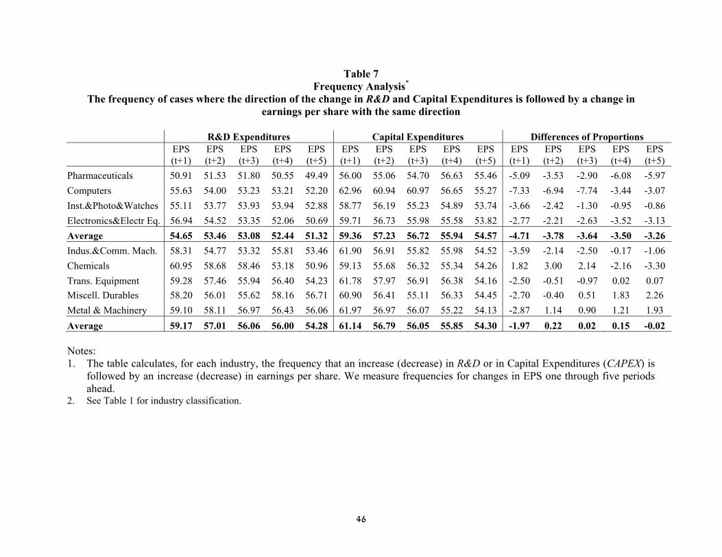
46
Table 7 Frequency Analysis*
The frequency of cases where the direction of the change in R&D and Capital Expenditures is followed by a change in earnings per share with the same direction
R&D Expenditures Capital Expenditures Differences of Proportions
EPS (t+1)
EPS (t+2)
EPS (t+3)
EPS (t+4)
EPS (t+5)
EPS (t+1)
EPS (t+2)
EPS (t+3)
EPS (t+4)
EPS (t+5)
EPS (t+1)
EPS (t+2)
EPS (t+3)
EPS (t+4)
EPS (t+5)
Pharmaceuticals 50.91 51.53 51.80 50.55 49.49 56.00 55.06 54.70 56.63 55.46 -5.09 -3.53 -2.90 -6.08 -5.97 Computers 55.63 54.00 53.23 53.21 52.20 62.96 60.94 60.97 56.65 55.27 -7.33 -6.94 -7.74 -3.44 -3.07 Inst.&Photo&Watches 55.11 53.77 53.93 53.94 52.88 58.77 56.19 55.23 54.89 53.74 -3.66 -2.42 -1.30 -0.95 -0.86 Electronics&Electr Eq. 56.94 54.52 53.35 52.06 50.69 59.71 56.73 55.98 55.58 53.82 -2.77 -2.21 -2.63 -3.52 -3.13 Average 54.65 53.46 53.08 52.44 51.32 59.36 57.23 56.72 55.94 54.57 -4.71 -3.78 -3.64 -3.50 -3.26 Indus.&Comm. Mach. 58.31 54.77 53.32 55.81 53.46 61.90 56.91 55.82 55.98 54.52 -3.59 -2.14 -2.50 -0.17 -1.06 Chemicals 60.95 58.68 58.46 53.18 50.96 59.13 55.68 56.32 55.34 54.26 1.82 3.00 2.14 -2.16 -3.30 Trans. Equipment 59.28 57.46 55.94 56.40 54.23 61.78 57.97 56.91 56.38 54.16 -2.50 -0.51 -0.97 0.02 0.07 Miscell. Durables 58.20 56.01 55.62 58.16 56.71 60.90 56.41 55.11 56.33 54.45 -2.70 -0.40 0.51 1.83 2.26 Metal & Machinery 59.10 58.11 56.97 56.43 56.06 61.97 56.97 56.07 55.22 54.13 -2.87 1.14 0.90 1.21 1.93 Average 59.17 57.01 56.06 56.00 54.28 61.14 56.79 56.05 55.85 54.30 -1.97 0.22 0.02 0.15 -0.02 Notes: 1. The table calculates, for each industry, the frequency that an increase (decrease) in R&D or in Capital Expenditures (CAPEX) is
followed by an increase (decrease) in earnings per share. We measure frequencies for changes in EPS one through five periods ahead.
2. See Table 1 for industry classification.