Graduate Theses, Dissertations, and Problem Reports

1999

Econometric analysis of household expenditures Econometric analysis of household expenditures

Samuel Berhanu West Virginia University

Follow this and additional works at: https://researchrepository.wvu.edu/etd

Recommended Citation Recommended Citation Berhanu, Samuel, "Econometric analysis of household expenditures" (1999). Graduate Theses, Dissertations, and Problem Reports. 3124. https://researchrepository.wvu.edu/etd/3124

This Dissertation is protected by copyright and/or related rights. It has been brought to you by the The Research Repository @ WVU with permission from the rights-holder(s). You are free to use this Dissertation in any way that is permitted by the copyright and related rights legislation that applies to your use. For other uses you must obtain permission from the rights-holder(s) directly, unless additional rights are indicated by a Creative Commons license in the record and/ or on the work itself. This Dissertation has been accepted for inclusion in WVU Graduate Theses, Dissertations, and Problem Reports collection by an authorized administrator of The Research Repository @ WVU. For more information, please contact researchrepository@mail.wvu.edu.

ECONOMETRIC ANALYSIS OF HOUSEHOLD EXPENDITURES

Samuel Berhanu

Dissertation Submitted to the College of Agriculture, Forestry and Consumer Sciences

at West Virginia Universityin partial fulfilment of the requirements

for the degree of

Doctor of Philosophyin

Natural Resource Economics

Dale K. Colyer, Ph.D., ChairTimothy T. Phipps, Ph.D.

Stratford M. Douglas, Ph.D.Gerard D’Souza, Ph.D.Laura Blanciforti, Ph.D.

Department of Agricultural and Resource Economics

Morgantown, West Virginia1999

Keywords: Household Expenditures, Budget Share, Expenditure Inequality Copyright 1999 Samuel Berhanu

ABSTRACT

An Econometric Analysis of Household Expenditures

Samuel Berhanu

While the traditional methods of measuring income inequality reveals interesting andimportant features of labor markets, estimates of income inequality do not provide completesummary statistics of the distribution of well-being. Interpreting the Gini coefficient of familyearnings as a measure of disparity in welfare implicitly assumes that households with the same levelof before tax income are equally well-off. Utility is derived from the consumption of goods andservices and there is ample empirical evidence which indicate that the distribution of totalexpenditure is likely to be different from the distribution of income. As Friedman indicatedhouseholds with low income levels are disproportionately represented by with those temporaryreductions in current income and will typically have high ratios of consumption to income.Households with high income levels are over represented by those with transitory increases inincome and will exhibit low ratios of consumption to income. The implication is that, all otherthings equal, one would expect less dispersion in the distribution of total expenditure relative to theincome distribution. The problems of using family income as a measure of well-being go beyondthe differences in the expenditure and income distributions. Treating heterogeneous householdssymmetrically, as is common in income inequality studies, indirectly assumes that two householdswith the same level of income but different sizes are equally well-off. If household characteristicsinfluences household expenditure patterns, consumption needs and welfare, such effects are likelyto have an important effect on both the level and trend of inequality in the distribution of welfare.Consumption rather than income may be a better measure of the actual economic welfare of ahousehold than its current income.

The main objectives of this study are to: 1. Measure the impact of demographiccharacteristics on the distribution of individual expenditures on the consumption of goods andservices. 2. Examine the inequality in the distribution of household consumption expenditures usingthe Gini coefficient.

The data are drawn from the 1980 through 1994 interview surveys conducted and gatheredby the U.S. Labor Statistics. An econometric method using the translog model is specified for sevencommodity groups. We estimated six equations using Seemingly Unrelated Regression procedure.

The parameters estimated to measure the impacts of demographic characteristics on theconsumption of goods and services indicated that the allocation of budget shares for differentconsumer goods is affected by the composition and characteristics of households. The decomposition of the Gini provides specific information concerning the concentration ofconsumption expenditures by budget components, and information about how the marginal changesin particular expenditures affect overall inequality. Unlike in income distribution, the Gini estimatesin expenditure distribution appear to be closer. It is possible to conclude that expenditure on goodsand services does depend not only on current income, but also on income earned through the years.This substantiates the permanent income hypothesis theory articulated by Friedman (1957). Beingable to measure these impacts can be useful for policy makers interested in the effect that certainprograms may have on the spending patterns of households. Results obtained in this studysubstantiate the importance of evaluating the differential impacts of proposed and enacted policies

on subgroups of the population and differences in inequality which can result when expenditures forbudget components change. Without adequate evaluation, policies and programs intended todecrease inequality may lead to the opposite outcome in the distribution of material well-beingacross household units in the population.

iv

ACKNOWLEDGMENT.

The task of conducting this research has been on of the most challenging and satisfying

experiences of my life. The completion of this work would have been impossible without the

generous advice, support and encouragement of many people.

The guidance and support of my committee members are greatly appreciated. Dr. Dale

Colyer, my committee chair provided practical and valuable knowledge of the subject, theoretical

and conceptual expertise. His professional advice and continuous encouragement, not only as the

chair of this committee, but also as a chair of my committee for my masters thesis will always be

valued. I also wish to acknowledge the contributions of the other members of my committee: Dr.

Gerard D’Souza, Dr. Tim Phipps, Dr. Strat Douglas, and Dr. Laura Blanciforti. Dr. Blanciforti

provided me with the opportunity to work on a project where I was privileged to obtain the data used

in this study. I have enormously profited from her expertise in the area of household budget and the

theory of demand systems. I am always grateful for her professional help and friendship.

I thank Lisa Lewis, Ellen Hartley, Gloria Nestor for their friendship and help. During my

doctoral program at WVU, I received funding from the Division of Resource Management and the

Regional Research Institute. I thank Dr. Luc Anselin, Dr. Scott Loveridge, Dr. Virgil Norton and Dr.

Peter Schaeffer for providing me with employment and financial assistance. Especially, Dr.

Schaeffer has played important roles in making the environment in the department more pleasant

and enjoyable. I am immensely grateful for his help and outstanding leadership.

Many other individuals have played various roles in making this difficult process more

pleasant. I am especially thankful for the friendship and unfailing support of Teferra Dinberu, Elias

Zewde and their families . Most importantly and with immense gratitude, I thank my good friends

v

Meselu Teferra and Zakarias Gebeyehu. They have practically demonstrated the true meaning of

friendship by standing with me during the bad and good times.

Finally, last but by no means least, a grateful kiss goes to my wife, Seble Hailu and my two

daughters, Rebecca and Leah for their unwavering love and support. Their devotion, patience and

understanding were indispensable.

I gratefully dedicate this piece of work to my late mother and father, Gete Mekonen and

Berhanu W. Mariam who instilled in me at an early age the importance of education and the value

of hard work. I only wish you could have been here to see me finish the journey I started with your

efforts and initiatives. I know you would have been so proud.

vi

TABLE OF CONTENTS

ACKNOWLEDGMENT. . . . . . . . . . . . . . . . . . . . . . . . . . . . . . . . . . . . . . . . . . . . . . . . . . . . . . . iv

CHAPTER 1: INTRODUCTION . . . . . . . . . . . . . . . . . . . . . . . . . . . . . . . . . . . . . . . . . . . . . . . . . 11.1 Background and Statement of the Problem. . . . . . . . . . . . . . . . . . . . . . . . . . . . . . . . . 11.2 Objectives . . . . . . . . . . . . . . . . . . . . . . . . . . . . . . . . . . . . . . . . . . . . . . . . . . . . . . . . . 61.3 Method and Organization. . . . . . . . . . . . . . . . . . . . . . . . . . . . . . . . . . . . . . . . . . . . . . 6

CHAPTER 2 LITERATURE REVIEW . . . . . . . . . . . . . . . . . . . . . . . . . . . . . . . . . . . . . . . . . . . . 82.1 Introduction . . . . . . . . . . . . . . . . . . . . . . . . . . . . . . . . . . . . . . . . . . . . . . . . . . . . . . . . . 82.2 The History and Development of Welfare Economics. . . . . . . . . . . . . . . . . . . . . . . 102.3 Conventional Ways of Measuring Income Distribution. . . . . . . . . . . . . . . . . . . . . . 26

2.3.1 Lorenz Curve . . . . . . . . . . . . . . . . . . . . . . . . . . . . . . . . . . . . . . . . . . . . . . . 272.3.2 Gini Coefficient. . . . . . . . . . . . . . . . . . . . . . . . . . . . . . . . . . . . . . . . . . . . . 302.3.3 Stochastic Dominance. . . . . . . . . . . . . . . . . . . . . . . . . . . . . . . . . . . . . . . . 392.3.4 An Income-Net Worth Approach. . . . . . . . . . . . . . . . . . . . . . . . . . . . . . . . 45

2.4 The Contributions of this Research. . . . . . . . . . . . . . . . . . . . . . . . . . . . . . . . . . . . . . 47

CHAPTER 3: THEORETICAL FRAMEWORK . . . . . . . . . . . . . . . . . . . . . . . . . . . . . . . . . . . . 493.1 Introduction . . . . . . . . . . . . . . . . . . . . . . . . . . . . . . . . . . . . . . . . . . . . . . . . . . . . . . . . 493.2 Aggregate Consumer Behavior. . . . . . . . . . . . . . . . . . . . . . . . . . . . . . . . . . . . . . . . . 493.3 Summary of Theoretical Considerations. . . . . . . . . . . . . . . . . . . . . . . . . . . . . . . . . . 613.4 Inequality in the Distribution of Household consumption Expenditure. . . . . . . . . . 64

CHAPTER 4: DATA AND DATA ORGANIZATION . . . . . . . . . . . . . . . . . . . . . . . . . . . . . . . 704.1 Introduction . . . . . . . . . . . . . . . . . . . . . . . . . . . . . . . . . . . . . . . . . . . . . . . . . . . . . . . . 704.2 Source of Data . . . . . . . . . . . . . . . . . . . . . . . . . . . . . . . . . . . . . . . . . . . . . . . . . . . . . . 704.3 Data Organization and Manipulation. . . . . . . . . . . . . . . . . . . . . . . . . . . . . . . . . . . . . 714.4 The Transformation of Time-Series-Cross Section Data to Panel Data. . . . . . . . . . 72

Chapter 5: Econometric Model and Estimation Results. . . . . . . . . . . . . . . . . . . . . . . . . . . . . . . 745.1 Introduction . . . . . . . . . . . . . . . . . . . . . . . . . . . . . . . . . . . . . . . . . . . . . . . . . . . . . . . . 745.2 Econometric Model. . . . . . . . . . . . . . . . . . . . . . . . . . . . . . . . . . . . . . . . . . . . . . . . . . 74

5.2.1 Dependent Variable Descriptions. . . . . . . . . . . . . . . . . . . . . . . . . . . . . . . . 755.2.2 Independent Variables. . . . . . . . . . . . . . . . . . . . . . . . . . . . . . . . . . . . . . . . . 75

5.3 Estimation and Empirical Results. . . . . . . . . . . . . . . . . . . . . . . . . . . . . . . . . . . . . . . 765.3.1 Food and Beverages. . . . . . . . . . . . . . . . . . . . . . . . . . . . . . . . . . . . . . . . . . 785.3.2 Housing and Housing Service. . . . . . . . . . . . . . . . . . . . . . . . . . . . . . . . . . . 815.3.3 Apparel. . . . . . . . . . . . . . . . . . . . . . . . . . . . . . . . . . . . . . . . . . . . . . . . . . . . 825.3.4 Entertainment. . . . . . . . . . . . . . . . . . . . . . . . . . . . . . . . . . . . . . . . . . . . . . . 845.3.5 Heath Care and Health Related Services. . . . . . . . . . . . . . . . . . . . . . . . . . 865.3.6 Transportation. . . . . . . . . . . . . . . . . . . . . . . . . . . . . . . . . . . . . . . . . . . . . . . 88

vii

5.3.7 Utilities . . . . . . . . . . . . . . . . . . . . . . . . . . . . . . . . . . . . . . . . . . . . . . . . . . . .905.4 Summary and Conclusions . . . . . . . . . . . . . . . . . . . . . . . . . . . . . . . . . . . . . . . . . . . . .91

5.4.1 The Impacts of the Age of the Head of the Household . . . . . . . . . . . . . . . .945.4.2 The Impact of the Size of Household . . . . . . . . . . . . . . . . . . . . . . . . . . . . .945.4.3 The Impacts of Geographic Location . . . . . . . . . . . . . . . . . . . . . . . . . . . . .965.4.4 The Impacts of Race . . . . . . . . . . . . . . . . . . . . . . . . . . . . . . . . . . . . . . . . . .97 5.4.5 Total Expenditure . . . . . . . . . . . . . . . . . . . . . . . . . . . . . . . . . . . . . . . . . . . .98

CHAPTER 6: INEQUALITY IN HOUSEHOLD CONSUMPTION EXPENDITURES . . . . . .996.1 Introduction . . . . . . . . . . . . . . . . . . . . . . . . . . . . . . . . . . . . . . . . . . . . . . . . . . . . . . . .996.2 The Gini Coefficient and Its Decomposition . . . . . . . . . . . . . . . . . . . . . . . . . . . . . . .996.3 Results and Discussions . . . . . . . . . . . . . . . . . . . . . . . . . . . . . . . . . . . . . . . . . . . . . .1026.4 Conclusion . . . . . . . . . . . . . . . . . . . . . . . . . . . . . . . . . . . . . . . . . . . . . . . . . . . . . . . .106

CHAPTER 7. SUMMARY AND CONCLUSION . . . . . . . . . . . . . . . . . . . . . . . . . . . . . . . . . .1187.1 Background . . . . . . . . . . . . . . . . . . . . . . . . . . . . . . . . . . . . . . . . . . . . . . . . . . . . . . .1187.2 Empirical Analysis . . . . . . . . . . . . . . . . . . . . . . . . . . . . . . . . . . . . . . . . . . . . . . . . . .120

7.2.1 The Impact of Demographic Characteristics . . . . . . . . . . . . . . . . . . . . . . .1217.2.2 Inequality in the Distribution of Consumption Expenditures . . . . . . . . . .123

7.3 Conclusions and Policy Implications . . . . . . . . . . . . . . . . . . . . . . . . . . . . . . . . . . . .1257.4 Limitations and Future Research . . . . . . . . . . . . . . . . . . . . . . . . . . . . . . . . . . . . . . .127

REFERENCES . . . . . . . . . . . . . . . . . . . . . . . . . . . . . . . . . . . . . . . . . . . . . . . . . . . . . . . . . . . . .131

Appendix . . . . . . . . . . . . . . . . . . . . . . . . . . . . . . . . . . . . . . . . . . . . . . . . . . . . . . . . . . . . . . . . . .141Appendix P-1: Program to Download Data and Create Data Set . . . . . . . . . . . . . . . . .142Appendix P-2: Program to Compute Expenditures by Month and Year . . . . . . . . . . . .174Appendix P-3: Rearrange the Month with the Year . . . . . . . . . . . . . . . . . . . . . . . . . . .177Appendix P-4: Program to Merge the Price File With the Expenditure Master File . . . 179Appendix P-5: Program to Display the Content of the Data Set . . . . . . . . . . . . . . . . . .180Appendix P-6: Program to Copy File . . . . . . . . . . . . . . . . . . . . . . . . . . . . . . . . . . . . . .181Appendix P-7: Program to Sort the Data Set . . . . . . . . . . . . . . . . . . . . . . . . . . . . . . . . .182Appendix P-8: Program to Compute Mean and Frequency . . . . . . . . . . . . . . . . . . . . . .183Appendix P-9: Program to Display Frequency Table . . . . . . . . . . . . . . . . . . . . . . . . . .184

viii

LIST OF TABLES

Table 5.1: Dependent Variables. . . . . . . . . . . . . . . . . . . . . . . . . . . . . . . . . . . . . . . . . . . . . . . . . . 75Table 5.2: Explanatory Variables. . . . . . . . . . . . . . . . . . . . . . . . . . . . . . . . . . . . . . . . . . . . . . . . . 76Table 5.3: Explanatory Dummy Variables. . . . . . . . . . . . . . . . . . . . . . . . . . . . . . . . . . . . . . . . . . 77Table 5.4: Food and Beverages. . . . . . . . . . . . . . . . . . . . . . . . . . . . . . . . . . . . . . . . . . . . . . . . . . 80Table 5.5: Housing and Housing Services. . . . . . . . . . . . . . . . . . . . . . . . . . . . . . . . . . . . . . . . . . 83Table 5.6: Apparel. . . . . . . . . . . . . . . . . . . . . . . . . . . . . . . . . . . . . . . . . . . . . . . . . . . . . . . . . . . . 85Table 5.7: Entertainment. . . . . . . . . . . . . . . . . . . . . . . . . . . . . . . . . . . . . . . . . . . . . . . . . . . . . . . 87Table 5.8: Health and Health Related Services. . . . . . . . . . . . . . . . . . . . . . . . . . . . . . . . . . . . . . 89Table 5.9: Transportation. . . . . . . . . . . . . . . . . . . . . . . . . . . . . . . . . . . . . . . . . . . . . . . . . . . . . . . 92Table 5.10: Utilities. . . . . . . . . . . . . . . . . . . . . . . . . . . . . . . . . . . . . . . . . . . . . . . . . . . . . . . . . . . 93Table 5.11: The Impact of Age of the Household (Compared to age 16-24 household. . . . . . . 95Table 5.12: The Impact of Size of the Household (Compared to single member household). . . 95Table 5.13: Impacts of Geographic Location of a Household (Compared to the Northeast). . . . 96Table 5.14: The Impact of Race (Compared to white). . . . . . . . . . . . . . . . . . . . . . . . . . . . . . . . . 97Table 5.15: The Impact of Total Expenditure on Share of Expenditures. . . . . . . . . . . . . . . . . . 98Table 6.1: Descriptions of Measures of Inequality. . . . . . . . . . . . . . . . . . . . . . . . . . . . . . . . . . 102Table 6.2: Signs for Ik - Sk . . . . . . . . . . . . . . . . . . . . . . . . . . . . . . . . . . . . . . . . . . . . . . . . . . . . . 105Table 6.3: Expenditure Inequality Effects by Expenditure Component for Year 1980. . . . . . . 107Table 6.4: Expenditure Inequality Effects by Expenditure Component for Year 1981. . . . . . . 108Table 6.5: Expenditure Inequality Effects by Expenditure Component for Year 1982. . . . . . . 108Table 6.6: Expenditure Inequality Effects by Expenditure Component for year 1983. . . . . . . 109Table 6.7: Expenditure Inequality Effects by Expenditure Component for Year 1984. . . . . . . 109Table 6.8: Expenditure Inequality Effects by Expenditure Component for Year 1985. . . . . . . 110Table 6.9: Expenditure Inequality Effects by Expenditure Component for Year 1986. . . . . . . 110Table 6.10: Expenditure Inequality Effects by Expenditure Component for Year 1987. . . . . . 111Table 6.11: Expenditure Inequality Effects by Expenditure Component for Year 1988. . . . . . 111Table 6.12: Expenditure Inequality Effects by Expenditure Component for Year 1989. . . . . . 112Table 6.13: Expenditure Inequality Effects by Expenditure Component for Year 1990. . . . . . 112Table 6.14: Expenditure Inequality Effects by Expenditure Component for Year 1991. . . . . . 113Table 6.15: Expenditure Inequality Effects by Expenditure Component for Year 1992. . . . . . 113Table 6.16: Expenditure Inequality Effects by Expenditure Component for Year 1993. . . . . . 114Table 6.17: Expenditure Inequality Effects by Expenditure Component for Year 1994. . . . . . 114Table 6.18: Expenditure Inequality by Age Using the Gini Coefficient. . . . . . . . . . . . . . . . . . 115Table 6.19: Expenditure Inequality Effects by Race Using the Gini Coefficient. . . . . . . . . . . 116Table 6.20: Income Inequality. . . . . . . . . . . . . . . . . . . . . . . . . . . . . . . . . . . . . . . . . . . . . . . . . . 117

ix

LIST OF FIGURES

Figure 2.1: Lorenz Curve. . . . . . . . . . . . . . . . . . . . . . . . . . . . . . . . . . . . . . . . . . . . . . . . . . . . . . . 28Figure 3.1: Gini Coefficient. . . . . . . . . . . . . . . . . . . . . . . . . . . . . . . . . . . . . . . . . . . . . . . . . . . . . 66Figure 6.1: Gini Coefficient for Total Expenditure, 1980-1994. . . . . . . . . . . . . . . . . . . . . . . . 107

1

CHAPTER 1: INTRODUCTION

1.1 Background and Statement of the Problem

The measurement of individual and household welfare stands out in applied welfare

economics for its ability to usefully combine economic theory with empirical practice. It is an area

where empirical study clearly relies on theoretical insight. There are important issues to be

addressed in identifying who lost and who gained as a result of complex policy implementations.

Potential Pareto improvements to societal welfare may not be known until the sizes of the gains and

losses are specifically measured or evaluated in some kind of quantitative unit.

In welfare economics, different considerations arise between the theoretical formulation of

a problem and the actual measurement of the effect of initiating a particular policy. Some theoretical

variables are not observable in the real world. For example, how does one measure a change in

conditions and how does one determine if the change is generally good or not. Measures showing

changes in income, wealth or expenditures are often used. However, these indicators are far from

precise and difficult to interpret for different circumstances. Alternative measures must be designed.

One observable alternative for measuring the intensity of individual preferences for a

situation is the amount of money the individual would pay or accept to move from one situation to

another (Just, Hueth and Schmitz, p.10, 1982). This principle has become the basis of modern

applied welfare economics. The two most important willingness-to-pay measures are compensating

(CV) and equivalent variations (EV). Based on the definition by Just, Hueth and Schmitz (p. 10-11,

1982) compensating variation (CV) is the amount of money, which when taken away from an

individual after a price and/or income change, will restore the individual’s original welfare level.

Similarly, equivalent variation is the amount of money given to an individual which if an economic

2

change does not happen leaves the individual as well off as if the change had taken place. In this

case the individual can be a consumer or producer. Thus, compensating and equivalent variations

are defined and perceived as mechanisms used to adjust the consumer’s income in order to maintain

his or her level of welfare. The compensating variation deals with the initial level of welfare, that

which the consumer held prior to price and/or income changes; and equivalent variation deals with

the subsequent level of welfare, that which the consumer would obtain with potential price and/or

income changes.

In most real world cases, public policies are enacted on a large number of people in a uniform

fashion. However, the determination of the policy effects on each individual decision unit is

impractical, both computationally and from the stand point of the availability of relevant data.

Generally, to perform a good welfare analysis of alternative policies, some aggregation is needed.

The welfare change measures discussed above are constructed on the assumption that all consumers

could be aggregated into a single representative consumer for welfare measurement purposes. The

conditions under which this can be done are very stringent. For one, it assumes that the marginal

social utility of income is identical for all persons, whether this results from a process of continually

redistributing income to maintain this equality, or whether this is a created assumption such as

marginal utility of income is the same for all households. The latter situation is straightforward in

the case where household indifference curve maps coincide. Failing either of these means that the

entire demand side of the economy could not be aggregated into a single individual from the social

point of view.

Nonetheless, most empirical studies using applied welfare economics proceed to measure

welfare change by simply aggregating CVs or consumer’s surplus over individuals. The question

3

naturally arises as to what interpretation can be given to the results of such exercises. The usual

argument is that the use of aggregated CVs to measure welfare change should not be interpreted as

measuring social welfare in any direct sense but, rather, it should be interpreted as indicating whether

or not there has been a potential improvement in social welfare. A potential improvement means

that the gainers from the change could hypothetically compensate the losers from the change while

remaining at least as well off after the change as before.

To obtain a measure of social change many consumer-economists rank all alternatives. The

ranking of social states involves making value judgements regarding measurability and comparability

which are not required when using the Pareto criterion or the compensation test. Although a social

welfare function is a desirable concept in theory, it does not exist in reality. As Just et al. (1982)

suggested, one should keep the concept of welfare economics in the background; but this does not

mean that one should totally forget the study of welfare economics just because the welfare function

cannot be specified in terms of any practical meaning. Even those who are critical of welfare

economics for the lack of defining a welfare function, must come to a consensus that it is often

possible to conclude who loses and who gains at least in monetary terms, as well as the magnitude

of these losses and gains, from specific policies, and that this information is crucial for policymakers.

Due to the problem of welfare aggregation and the non-existence of the social welfare function, we

are forced to rely on imperfect measures of welfare such as income distribution, wealth distribution

and expenditure functions.

There are a number of ways of characterizing income distributions. These are often used as

summary statistics for evaluating inequality in the distribution of income or for evaluating the

distributive impact of, say, tax policy changes. They include the Gini coefficient, or its graphical

4

counterpart the Lorenz curve, the variance of income, the relative mean deviation, the standard

deviation of logarithms of incomes, and the like.

Similarly, a money metric of utility, such as an expenditure function, has a role in measuring

social welfare. The utility of an individual may be written as a function of a money metric

representing the expenditure function. Indifference curves can uniquely define utility associated with

the expenditure function. Utility can be written or defined as a function of expenditures given the

reference price vector. Based on this definition, the value of the indirect utility of the consumer at

the reference prices, given that utility is, fully measurable. Social welfare may be written as a

function of the individual expenditure function at a given set of reference prices. The measurement

of social welfare can proceed by using the appropriate aggregation of the money metric measures of

utilities rather than the utilities themselves. There are also a variety of other imperfect methods to

measure welfare changes, in addition to the ones discussed above.

While the investigation of inequality using the imperfect methods observed above reveals

interesting and important features of the market, estimates of inequality are not particularly

informative summary statistics of the distribution of well-being in the United States. For example,

interpretation of the Gini coefficient of family income as a measure of dispersion in welfare

implicitly assumes that families with the same level of before tax income are equally well-off.

However, utility is derived from the consumption of goods and services and there is ample evidence,

emanating from Friedman’s (1957) permanent income hypothesis, which suggests that the

distribution of total expenditures is likely to be quite different from the distribution of incomes.

According to Friedman, households with low income levels are disproportionately represented by

those with temporary reductions in current income and will typically have high ratios of consumption

5

to income. Households with high income levels are over represented by those with transitory

increases in income and will exhibit low ratios of consumption to income. The implication is that,

all other things equal, one would expect less dispersion in the distribution of total expenditures

relative to the income distribution.

The problems created as a result of using family income as a measure of well-being go

beyond the differences in income and expenditure distributions. Households have different

characteristics. Treating heterogeneous households symmetrically, as is common in income

inequality examination, indirectly assumes that two households with the same level of income but

different sizes and demographic characteristics are equally well-off. If household composition

influences household expenditure patterns, needs and welfare, such effects are likely to have an

important impact on both the levels and trends of expenditures and inequality in the distribution of

welfare.

Using family income as a measure of household welfare also ignores the potential impact of

prices on the distribution of well-being. Increases in the prices of basic necessities relative to

luxuries will hurt the poor relatively more than the rich and increase the disparity in welfare. The

large increase in the relative prices of energy goods in the 1970s could have had a substantial impact

on the relative welfare levels. Looking at the distribution of family income alone would obviously

ignore the above effect.

One of the goals of this study is to use a different methodology for measuring inequality in

the distribution of welfare, one which is operationally feasible and broader in scope than the

traditional money income measure. This approach to inequality measurement is based on the theory

of exact aggregation developed by Lau (1977). One of the important implication’s of Lau’s theory

6

of exact aggregation is that systems of demand functions for individuals with common demographic

characteristics can be recovered uniquely from the system of aggregate demand functions. By

requiring that the individual demand functions be integrable, it is possible to recover the indirect

utility functions for all consumers. Finally, measures of individual welfare can be defined in terms

of these indirect utilities. The model used in this study incorporates pseudo-panel micro data on the

allocation of consumer expenditures due to different demographic consumer characteristics.

1.2 Objectives

The overall of goals of this study are to provide information on inequality in the distribution

of household consumption expenditures and to measure the impact of demographic attributes of a

household on consumption expenditures. The specific objectives are to:

1. Measure the impact of demographic characteristics on the distribution of individual

expenditures on the consumption of goods and services in the United States between 1980

and 1994.

2. Evaluate the changes in individual household expenditures across demographic subgroups.

3. Examine the inequality in the distribution of household consumption expenditures using

the Gini coefficient. Gini coefficients will be calculated for commodity components and

demographic subgroups of the population defined in terms of household composition, the

race, age of the reference person, and region of residence.

1.3 Method and Organization

Chapter 2 presents a review of related literature and is divided into 4 sections. An

introduction is given in section 2.1 followed by section 2.2 addressing the history and development

of welfare economics. The conventional ways of measuring income distribution are presented in

7

section 2.3. A discussion on the expected contribution of this study is given in section 2.4. The

theoretical framework to address the development of empirical models for this topic is addressed in

sections 3.2 and 3.4 of chapter 3. The data set used in this study is discussed in chapter 4. This data

set is developed from a BLS consumer expenditure survey. In section 5.2 of chapter 5, the

econometric methodology for developing a model to measure the impact of demographic

characteristics on household consumption expenditures is outlined. In section 5.3 of the same

chapter, the implementation of the econometric model, its results, and detailed discussions are

presented. In chapter 6, section 6.2 the method for measuring the inequality of household

consumption expenditures is presented. The estimates are presented and broad discussions of the

results are reported in section 6.3.

Finally, a summary, conclusions, limitations of the study, and a discussions of future research

needs are presented in chapter 7.

8

CHAPTER 2 LITERATURE REVIEW

2.1 Introduction

The measurement of inequality has long concerned writers in the field of personal income

distribution. Interest in measurement of income inequality and level of poverty can be traced to as

early as 1890, when the development of a poverty line was discussed by Charles Booth. Economists

are well aware that money income is not a completely accurate indication of relative standard of

living. But most people interested in the issue of inequality base their perception of the degree of

economic inequality on the Census Bureau’s data on the distribution of money income. The

underlaying issues of measuring the economic status of families and defining the poor remain to be

settled. The effects of these problems are detrimental if the intention is to provide uniform

treatment to families of equivalent economic status. For example, government programs directed

at poor families often intend to include all those who are poor and to totally exclude those who are

not. When receipt or denial of very much needed benefits is decided by a single empirical index, it

is obviously important for that index to conform to a generally shared view of both horizontal and

vertical equity. Hugh Dalton, in the preface to The Inequality of Income (September 1920), referred

to the ambiguity of the conception of inequality and the need to give it a more precise definition and

a logical measure (Atkinson, 1983). Dalton, in this pioneering article on the measurement of

inequality, took issue with earlier researchers who had suggested that the position of an economist

choosing a measure of inequality was identical to that of a biologist in determining the distribution

of a physical characteristic (Atkinson, 1983). Dalton (1920, p. 348) argued that:

This is clearly wrong. For the economist is primarily interested, not in the

distribution of income as such, but in the effect of the distribution of income upon

the distribution and total amount of economic welfare, which may be derived from

9

income.

The above statement of Dalton did not receive the attention which it deserved for many years

(Atkinson, 1983). Empirical work on income and wealth inequality continued to use summary

indicators of inequality, such as the mean deviation of the Gini coefficient, which were statistical in

origin rather than derived from considerations of social welfare. It was, indeed, nearly fifty years

later that Serge Kolm (1969) independently raised Dalton’s approach and argued for a

reconsideration of the measurement of inequality. These contributions led in turn to a very

substantial literature on the underlying and basic conceptual issues.

Cash income is the most commonly used indicator of economic status, but it is widely

recognized that this measure is inadequate. Comparisons using a cash income measure may not

assure horizontal equity since other consumable resources may be missing. For some families

current cash receipts constitute only a small portion of the available sources of economic welfare.

Differing amounts of in kind transfers and physical and human capital can substantially change the

economic status of families with similar cash incomes, causing them to no longer be as equals. For

this reason, other sources of resources are often included to create alternative indices of family status.

Moreover, vertical equity considerations--the ranking of the families and the equality of the

distribution are more likely to be affected. Wealth, family size, location of residence, disability,

income variability, and age are often introduced to alter the rankings that result from using either

cash income alone or some expanded definition of economic welfare.

The need for a more expansive and accurate measure of economic status for descriptive,

analytic, and policy purposes is obvious if standards are to be identified. The place to start, perhaps,

is the theory of welfare economics, since measurement of inequality falls in the study of welfare

10

economics. Welfare economics is a branch of economics developed to help society make better

choices (Just et al., 1982). The measurement of individual and household welfare stands out in

applied welfare economics for its capability to usefully blend economic theory with empirical

practice (Blundell et al., 1994). It is an area where empirical investigation clearly benefits from

theoretical insight and where theoretical concepts are brought alive and appropriately focused by the

discipline of empirical relevance and policy design (Blundell et al., 1994). Yet there are many

unanswered questions in identifying who gains and who loses from complex policy initiatives. This

is exactly the problem to which this study is directed. A good measure of well-beingness is required

for successful policy implementation.

This chapter has three more sections. The summary of the history of welfare economics and

related theoretical and empirical developments is presented in section 2.2. Section 2.3 addresses the

traditional methods of the measurement of income inequality and gives a summary of literature in

this area. The third section, 2.4, discusses the potential contributions this research will make in field

of income and welfare distribution.

2.2 The History and Development of Welfare Economics

An answer to the question of the method and content of normative economics, and more

precisely welfare economics, can be made to turn on historic analysis. What for instance, did

Marshal (1920), Pigou (1946), Little (1957), Graaf (1957), and many others, mean when they wrote

about welfare economics? There is much conflict between what the better known writers have meant

by welfare economics and its understanding among the profession today. Differences between the

conclusions reached by the older tradition associated with Marshal, Pigou, Robertson, and to some

extent Lerner (1946), as distinguished proponents of the Cambridge or Neoclassical School--which

11

is built on a foundation of diminishing marginal utility and a belief in a basic similarity of human

beings and a more modern approach, associated with the names of Vilfredo Pareto (1896), Hicks

(1939), Samuelson (1950), and many others, turn out to be significant only with respect to

distributional propositions. With respect to the purely allocative analysis, there is a general

agreement, although with the passage of time there is a greater appreciation today of its limitations.

We adopt what is today the more popular approach to the subject, building on the foundation laid

by Bergson (1938), Kaldor (1939), and Hicks (1939) from whence sprang modern welfare

economics; there will be little difficulty in pointing out, from time to time, certain differences in

premises and conclusions between the older neoclassicist treatment and the more modern treatment.

Often, a distinction is made between the old welfare economics of Marshal et al. and what

has come to be called the new welfare economics. The old welfare economics accepts the principle

that social gains are maximized by competitive markets and, therefore, where noncompetitive

interferences exist, the economist is justified in recommending policy measures that eliminate those

distortions (Just et al., 1982). Also, the old welfare economics employs the technique of partial-

equilibrium analysis in developing recommendations. Partial-equilibrium or piecemeal analysis

considers the welfare effects of a change in one market, assuming the effects in other markets are

negligible (Just et al., 1982). From an empirical stand point, the old welfare economics holds that

the triangle like area to the left of the demand curve and above price (often called consumer surplus)

is a serviceable money measure of utility to the consumer in a market and that a triangle like area to

the left of the supply curve and below price (producer’s surplus) is similarly an adequate money

measure of welfare for producers in a market (Just et al., 1982). Changes in these areas can be used

to measure welfare changes to society.

12

The principles of the old welfare economics have been attacked on several grounds by those

economists associated with the new welfare economics. For example, beginning in 1942,

economists such as Paul A. Samuelson demonstrated that the basic welfare measure of the old

welfare economics--consumer surplus--is not well defined (Just et al., 1982). That is, consumer

surplus is not generally a unique money measure of utility; uniqueness can imply contradictions

depending on the use of empirical data. This criticism of the use of consumer surplus put applied

welfare economics on somewhat shaky grounds until Willig’s work appeared in the mid 1970's (Just

et al., 1982).

Another criticism of welfare economics is based on an argument advanced as early as 1896

by Pareto. He argued that any policy that makes any person worse off cannot be supported on

objective grounds. As further elaborated by Hicks and Kaldor, the welfare weight attached to each

individual need not be the same and, hence, simply summing changes in consumer or producer

surpluses across individuals is not a sufficient basis for evaluating change. Pareto argued that the

only objective basis under which one can say society is better off is when some people are made

better off and no one is made worse off. This criterion has come to be known as the Pareto principle.

In an attempt to extend the class of questions that can be addressed objectively by welfare

economics, Hicks and Kaldor introduced the compensation principle in 1939 by which a change

should be made if potential gain exists so all could be made better off by some redistribution of

goods or income following the change (Just et al., 1982). The associated measurement problem was

addressed by Hicks who suggested that alternative money measures of welfare, while not directly

related to utility gains and losses, can be given willingness to pay interpretations (Just et al., 1982).

These measures, known as compensating and equivalent variations, are unique measures in any

13

situation and are hence not subject to the Samuelson criticism of consumer surplus (Just et al., 1982).

The notion of compensating and equivalent variations and the associated compensating criteria are

key concepts and form the foundation of applied welfare economics.

But even the compensating principles did not escape criticism. Scitovsky, in what has

become known as the reversal paradox, illustrated how inconsistencies can arise in using this

principle in policy analysis. Later, Gorman extended this analysis to illustrated the intransivity

problem associated with inconsistent rankings of three or more situations (Just et al., 1982).

Applied welfare economics have been used extensively in recent years as though (if not

actually) innocent of the controversy. Applied welfare economists continued to use partial

equilibrium models for policy recommendations; and some recommendations have been

legislatively mandated. The Flood Control Act of 1936 required that the benefits from water

resource development projects must exceed the costs regardless of to whomever either may accrue

(Just et al., 1982). To measure these benefits and costs in project evaluation work, economists

continue to use the areas behind supply and demand curves. Policy makers demand economic

analysis of policy decisions and applied welfare economists have used the only tools they have had

available to provide information (Just et al., 1982).

Fortunately, however, some theoretical justification for feasible empirical work practices

have followed. For example, the piecemeal approach has been shown to be appropriate when some

markets or sectors have little economic impact on others. Where market interdependence exists,

welfare economists now have better guidance as to how far they need to look to obtain the total

welfare effects of a policy change. Similar advances have been made in other areas and under other

assumptions. A number of important issues have characterized the recent literature on the

14

measurement of welfare: how to incorporate differences in household characteristics into welfare

evaluation; how to evaluate the welfare of individuals when they live in households; the potential

for using subjective survey data for measuring welfare; and how to measure social welfare, inequality

and poverty from individual welfare measures (Blundell et al., 1994).

One of the key concepts in economics is utility or welfare. The first thorough introductions

of the concept were those by Gossen (1854) and Jevons (1871) and Edgeworth (1881). They

assumed, using modern jargon, that a commodity bundle x in the commodity space (�+) contains the

intrinsic utility value (Ux). The consumer problem could then be described as looking for the bundle

with the highest utility value that could be bought at prices p and income y (Van Praag, 1994). Such

a model is capable of describing and predicting the purchasing behavior of an individual. Actually,

this is the behavioral aspect of the model. According to Van Praag the model can also be used for

normative purposes, where we compare utility differences between bundles x1, x2, x3 for a specific

individual. The utility of income levels y1, y2, y3 may be calculated by means of the indirect utility

function V(y,p) which is defined as the maximum utility to be derived from income y at given prices

p. It also would be possible to define a social welfare function, W(U1,.......,Un), where social

welfare is a function of individual utilities. The most common application of that concept is to

compare distributions of social wealth and design policies which may lead to a better distribution.

Pareto (1909) gave a fierce blow to the utility concept by showing that demand behavior was

completely determined by the contour lines, defined by the equation U(x) = constant (Van Praag,

1994; Just et al., 1982). The result is that demand behavior does not define the utility function

uniquely, but rather that there is a whole equivalence class of utility functions which yields the same

demand behavior. Those utility functions have a property that � = �(U) where �(.) is any

15

monothonically increasing function (Van Praag, 1994). This eroded utility concept is called the

ordinal concept. The original one of, for example, Edgeworth is called the cardinal utility concept.

Pareto (1909) did not state that cardinal utility was a nonsensical concept but only that it was not

necessary to know the utility function to explain demand behavior, as knowledge of the contour lines

of the utility surface on the commodity space is all that is needed (Kirman, 1987).

Robbins (1932) made a fierce attack on cardinal utility and stated that it was an unmeasurable

concept altogether. Hicks and Allen (1934) and later Houthakker (1950) gave rigorous explanations

of demand behavior without applying the utility concept at all. Deaton and Muellbauer (1982) made

similar observations. So, the utility concept degenerated to a handsome tool to describe choice

behavior. However, during the last thirty years the number of economists disagreeing with Pareto

has been increasing. Several attempts at measurement or developing methods of possible

measurement of utility have been made. The procedure can be described by the assumption that

utility is the same function of a number of determinants or components for all individuals or

households but with parameters characterized by the individual being considered which differ among

individuals (Jorgenson and Slesnick, 1984). Thus, in recent years, major empirical measurements

were made by three different groups of economists American, Dutch, and French groups.

The American group, which is made up of Christensen, Jorgenson, Slesnick, and Stocker,

use a translog utility function, that is, one where the log utility is a quadratic function of the log of

determinants and the latter are three or five consumption goods or services. The number of

parameters to characterize the groups of consumers is also five: family size, age of head, region of

residence, race, and type of residence. They introduce restrictions on preferences not used by

ordinalists which may be considered the price they pay to justify being cardinalists. The restrictions

16

w � �i

�i ln(xi � 1) (2.1)

�w�xi

�

�i

(xi � 1)(2.2)

used are exact aggregation of individual demand to total demand and the integrability of demand

functions rather than formal criteria.

The Dutch economists are led by Van Praag and Kapteyn. They use one determinant, income

and test a large number of utility functions, although they prefer the cumulated lognormal function,

for reason of convenience in a number of applications (Van Praag, 1971; Kapteyn, 1977; Van

Herwaarden and Kapteyn, 1981). The function they prefer is linear in the logs of determinants xi,

plus unity:

The advantage of this relationship is that it shows falling marginal utilities, namely:

The general restriction implies that the qualifications used to carry out the measurement procedure

of the satisfaction experienced have the same meaning to the person compared. This restriction can

be accepted since, in discussion on the policy resulting from the use of welfare measurement, the

same words are also used either to accept or reject the policy. The restriction can be applicable only

on a local or national level, rather than on international level, because the concept of a good income

means something different to, say, an American and a Chinese metal worker.

The French economist who engaged in measuring welfare is Maurice Allias. He uses one

component, psychological assets, and prefers the functional shape of linearity in its log (Allias,

1984). He only claims this shape for the main interval of the variable and admits that deviations

17

occur at the extremes. At the upper extreme he finds the phenomenon of satiety (an asymptote).

Measuring welfare or utility has become a respectable activity among many economists, and

is considered to be comparable to similar processes and developments in other sciences. Clear

examples can be found in physics where initially qualitative characteristics were followed by very

satisfactory quantitative measurements. In the theory of heat qualification, qualitative values such

as hot, warm, luckwarm, and cold were later replaced by specific temperature. In the theory of light,

qualitative characteristics such as red, orange, yellow, green, blue, and purple were replaced by wave

length. In the theory of sound and music, wave lengths also became characteristics of low and high

sounds.

One way to measure economic status as suggested by Peter Hammond (1976) is to do

interpersonal comparisons. Interpersonal comparisons can be of utility levels and/or utility

differences. Comparisons of levels can be used to define equity in the distribution of income. Sen

(1973) gives a particular example by a thorough and interesting discussion of the welfare economics

of income distribution in his book, On Economic Inequality. At the beginning of this book,

utilitarianism is criticized on the grounds that it may lead to choices of income distribution which

conflict with the notion of equity (Sen, 1973). He emphasized how one can make interpersonal

comparisons of utility differences.

Hammond (1976), instead, set out to find an equity-regarding additive Bergson social welfare

function, taking account of both types of comparisons. He further explains (p. 70):

It may not exist unless the interpersonal comparisons satisfy certain restrictions. The

precise nature of these restrictions depends upon the precise nature of the dual

interpersonal comparison. The most restrictive case is the one which Sen considered,

18

where both levels and differences of a single list of consumers� utility functions are

being compared. In the least restrictive case, the level of one list of utility functions

and the differences of a quite separable list of utility functions are compared. There

is a third, intermediate case, where one compares the levels of a list of utility

functions and the differences of a cardinally related but different list of utility

functions.

If the price vector is considered along with the distribution of income, then dual interpersonal

comparability may restrict the form of the consumers� indirect utility functions (Hammond, 1976).

Hammond goes on to say (p.70):

In the most restrictive case, the restrictions imply that any one consumer�s Engle

curves can be obtained from any other consumer�s Engle curves by way of simple

lateral shift. The property needed for consistent aggregation, the Engle curves are

parallel straight lines, emerges as special case. The intermediate kind of dual

comparability gives somewhat weaker restrictions; the least restrictive kind of dual

comparability puts no restriction at all on consumers� indirect utility functions, or on

their demand functions.

Hammond (1976) points out that market data helps to determine the precise form of the

welfare function.

Muellbauer (1974a) analyzed household composition, Engle curves and welfare comparisons

between households using a duality approach. The household composition effects in consumer

theory are important for the specification and estimation of Engel curves and demand functions. The

models examined by Muellbauer (1974a) have important applications in the areas of measurement

19

of cost of living indices, the study of poverty and equality and in certain aspects of social policy.

These models are based on the approach of Barten (1964). In his study, test differences between

households are parameterized in a way which has been called simple good augmenting or simple

repackaging in the literature on equality change--see Fisher and Shell (1967) and Muellbauer

(1973a). In this theory, changes in household composition play an analogous role to price changes.

Barten (1964) suggests that price elasticities might be estimated from cross-section data alone.

The indices introduced are of considerable importance in analyzing poverty and inequality

(Muellbauer,1974a). Unless household composition is taken into account in this way, it makes

virtually no sense to compare the money incomes of different households. Recently Atkinson (1970)

and Sen (1973), among others, have discussed measures of inequality. As far as operational

measures are concerned, this always boils down to measures of money inequality and it is always

assumed that the individual utility functions are identical (Muellbauer, 1974a). Clearly, this is

inadequate for households. However, with the above theory, the approach of Atkinson and Sen can

be extended to measure economic inequality between households. Muellbauer states that the Engel

method is painfully devoid of any micro-economic theoretical basis and continues in use only

because recent advances in the basic theory of consumption economics have not been applied to the

estimation of equivalence scale.

Still on the subject of welfare comparison, Pollak and Wales (1979) addressed the distinction

between the equivalence scale required for welfare comparisons and the equivalence scale which

arises in demand analysis. Of course, equivalence scales are used in both demand and welfare

analyses. In demand analysis they permit us to pool data from households of different sizes, or more

generally, with different demographic profiles. In welfare analysis, they enable comparison of the

20

well-being of such households, since they purport to answer questions of the form: what expenditure

level would make a family with three children as well off as it would be with two children and

$12,000? According to Pollak and Wales (1979) such welfare comparisons are generally thought

to provide the rationale for different treatments of different family types in income tax or family

allowance schedules, or in an income maintenance program (Pollak and Wales,1979).

The authors also explicitly pointed out the types of equivalence scale appropriate for demand

analysis or welfare comparisons. Conditional equivalence scales are used in demand analysis while

unconditional equivalence scales are used for welfare comparisons. Conditional equivalence scales

can be estimated from observed differences in the consumption patterns of households with different

demographic profiles, but construction of unconditional equivalence scales requires more

information than is contained in household consumption data (Pollak and Wales, 1979).

Pollak and Wales (1979) explicitly stated the implications of their analysis of welfare

comparisons and equivalence scales as:

1. Even if all families have identical unconditional preferences, conditional

equivalence scales estimated from observed differences in the consumption patterns

of families with different demographic profiles cannot be used to make welfare

comparisons; for example, we cannot use such data to determine the amount needed

to make families with three children as well off as those with two children and

$12,000. Unconditional equivalence scales are required to make welfare

comparisons.

2. If tastes vary systematically with demographic characteristics, then the

construction of unconditional equivalence scales requires the selection of an

21

appropriate base unconditional preference ordering; theory offers little guidance in

making this selection, but there is no selection which permits us to compare the

welfare of a family with a strong desire for children with that of one with a weak

desire for children. Such comparisons require interpersonal or inter family

comparisons of welfare levels.

Slesnick (1994) empirically demonstrated that the distribution of expenditures is different

from the distribution of income. The paper also assesses the robustness of the widely accepted

conclusion that inequality in the United States has reversed course and attained unprecedented (high)

levels. The author avoided the problems associated with money income inequality studies by using

a measure of welfare that is based on consumption level and incorporates the needs of households,

as well as the influence of prices. It came out that the distribution of a consumption based welfare

measure is different from the family income distribution, which is used to demonstrate rising

inequality in the United States (Slesnick, 1994). The result points out that income performs poorly

as a proxy for household welfare in measuring inequality (Slesnick , 1994). Further, Slesnick found

that income inequality overstates consumption based on inequality measures by a substantial

amount. The trends and consumption based on inequality indexes also diverge, with income

measures indicating rising inequality over the postwar United States and the consumption measure

showing the reverse.

What accounts for the difference between the distribution of before tax income and the

distribution of real per equivalent expenditure? The answer given by Slesnick is that the distribution

of total expenditure is less dispersed than the distribution of income which, in turn, appears to be the

result of consumption smoothing across the population. The inclusion of household needs in the

22

evaluation of welfare is also an important component in accounting for the differences in the levels

and trends of inequality in the United States.

The focus of attention of policy makers and researchers has been the U-turn in income

inequality in the United States. But Slesnick’s findings indicate that when household welfare is

measured using real per equivalent expenditures, the level of inequality fell until the early 1970s and

has remained essentially constant thereafter. However, in 1991 the level of inequality remains high

so that substantial gains in social welfare can be had through further equalization of the distribution

of welfare. The suggestion given on policy issues is that it is perhaps more useful to focus attention

on the forces that induced the reduction in inequality rather than try to explain the illusory U-turn

in inequality that occurred in the 1970's and 1980's.

On a related topic Blundell, Browning and Meghir (1994) estimated the parameters of

household preferences that determine the allocation of goods within the period and over the life-

cycle, using micro data. In doing so, they were able to identify important effects of demographic,

labor market status and other household characteristics on the intertemporal allocation of

expenditures. The distinctive feature of their approach is that it integrates traditional demand

analysis with an intertemporal substitution model in a coherent way.

Based on the author’s suggestions, the findings of this type of research is open to a variety

of interpretations which cannot be distinguished convincingly within this framework. First, it is

quite possible that the importance of labor market variables in the intertemporal model does in fact

reflect a shift in tastes as a function of labor market status; since labor market status and the growth

rate of income are obviously correlated ignoring the former makes the later spuriously significant

(Blundell, Browning and Meghir, 1994). Further, they point out that for the same reason labor

23

market status is a good predictor of income growth and, thus, labor market status may just capture

excess sensitivity. In a recent empirical finding, Jorgenson and Slesnick (1984) were able to

measure welfare inequality based on an econometric model of aggregate consumer behavior. This

model allows them to uniquely recover systems of individual demand functions from the systems

of aggregate demand functions. By requiring that individual demand functions be integrable, they

recovered indirect utility functions for all consumers (Jorgenson and Slesnick, 1984). As a result,

they were able to define measures of individual welfare in terms indirect utility functions.

To represent preferences for all individuals in a form suitable for measuring individual

welfare, households are taken as consuming units. It is also assumed that expenditures on individual

commodities are allocated so as to maximize welfare functions. As a result, the household behaves

in the same way as an individual maximizing a utility function, as demonstrated by Samuelson

(1956) and Pollak (1981). By assuming that each household maximizes a household welfare

function, the focus can be on the distribution of welfare among households (Jorgenson and Slesnick,

1984). An econometric model based on exact aggregation can be defined through representing

individual preferences by means of an indirect utility function for each consuming unit (Jorgenson

and Slesnick, 1984). They also assume the kth consuming unit allocates expenditures in accordance

with the translog indirect utility function. By applying Roy�s identity, the system of individual

shares is obtained. Aggregate expenditure patterns depend on the distribution of expenditures over

all consuming units through summary statistics of the joint distribution of expenditures and attributes

(Jorgenson and Slesnick, 1984). The first step in analyzing inequality in the distribution of

individual welfare is to select a representation of the individual welfare function. The assumption

is that the individual welfare of the kth consuming unit is equal to the logarithm of the indirect utility

24

function. The indirect utility function provides a cardinal measure of utility. If a system of

individual expenditure shares can be generated as an indirect utility function, we can say that the

system is integrable. A complete set of conditions for integrability is given by Jorgenson and

Slesnick (1984):

Homogeneity The individual expenditure shares are homogeneous of degree zero in prices and

total expenditure.

Summability: The sum of the individual expenditure shares over all commodity groups is equal to

unity.

Symmetry: The matrix of compensated own- and cross-price substitution effects must be symmetric

Nonnegativity: The individual expenditure shares must be nonnegative.

Monotonicity: The matrix of compensated own-and cross-price substitution effects must be non-

positive definite.

To provide a basis for evaluating the impact of transfers among households on social welfare,

it is useful to represent household preferences by means of utility functions that are the same for all

consuming units. Consumer equilibrium implies the existence of an indirect utility function that is

the same for all consuming units. The level of utility for the kth consuming unit depends on the

price s of individual commodities, the household equivalence scale, and the level of total

expenditures (Jorgenson and Slesnick, 1984). The first step in analyzing inequality in the

distribution of welfare is to select a representation of the individual welfare function. Jorgenson and

Slesnick (1984) assume that the individual welfare for the kth consuming unit is equal to the

logarithm of the translog utility function. The next step is to generate a social welfare function that

has the properties of an unrestricted domain, independence of irrelevant alternatives, positive

25

association, nonimpostion, and cardinal full comparability (Jorgenson and Slesnick, 1984). They

impose the additional assumption that the degree of aversion to inequality is constant and require

the social welfare function to satisfy requirements of horizontal and vertical equity.

To develop indexes of inequality in the distribution of individual welfare, Jorgenson and

Slesnick (1984) decompose the measure of social welfare into measures of efficiency and measures

of equity. Efficiency can be defined as the maximum level of welfare that is potentially available

through redistribution of aggregate expenditures. The absolute level of inequality is defined as the

difference between the measure of efficiency and the actual level of social welfare. Also, a relative

measure of inequality is defined as the ratio between the absolute index of inequality and the

measure of efficiency. The decomposition of social welfare into measures of efficiency and equity

takes place through the maximization of social welfare for a fixed level of aggregate expenditure.

The average level of individual welfare for a given level of aggregate expenditures can be maximized

by means of the Langrangian.

If aggregate expenditure is distributed so as to equalize total expenditures per household

equivalent member, the level of individual welfare is the same for all consuming units. Equivalent

member is a member of a household for which expenditure is allocated based on an index called

equivalent scale. Equivalent scale is an index which deflates family income or expenditure by a

score that may be less than one for each extra member. This is the maximum level of welfare that

is potentially available and can be taken as a measure of efficiency. We can refer to this measure

as the translog index of efficiency. The translog index is equal to the translog indirect utility

function, evaluated at aggregate expenditure per household equivalent member for society as a whole

(Jorgenson and Slesnick, 1984).

26

Given the translog index of efficiency defined in terms of the social welfare function, we can

define a measure of inequality as the difference between the translog index of efficiency and the

actual value of the social welfare function (Jorgenson and Slesnick, 1984). We can refer to this

measure as the translog index of inequality. Likewise, it is possible to develop a measure of

inequality within subgroups of the U.S. population. For this purpose, a group welfare functions are

introduced that are precisely analogous to the social welfare function discussed earlier. A group

welfare function can be defined as a mapping from the set of individual welfare functions to the set

of group orderings(Jorgenson and Slesnick, 1984). A group ordering can be described in terms of

properties of a social welfare function. The same steps can be taken to decompose a group welfare

function into measures of efficiency and equity. As a result, measures of inequality within groups

are obtained.

2.3 Conventional Ways of Measuring Income Distribution

The distribution of income is one of the main features of any social system. David Ricardo,

the classical economist par excellence, regarded the determination of income distribution as the most

important task facing economics. This view is no longer widely held in the face of today’s problems

(unemployment, inflation). Nevertheless, stagnation in economic growth in virtually all modern

industrialized societies, which has became the subject of public debate recently, has meant increasing

pressure for more attention to be paid to the distribution of the national pie.

Theoretical success in the study of personal income distribution is still modest. None of the

existing theories are entirely satisfactory. Money income is what we observe and tax. But it is not

completely satisfactory indicator of well-being. Throughout the last fifty years numerous

measurement methods have been employed to measure the distribution of income. This section

27

�(x) � �x

0g(r)dr (2.3)

Q(x) � �x

0rg(r)dr (2.4)

reviews and discusses some of the methods used and some of the articles and books published on

this particular topic.

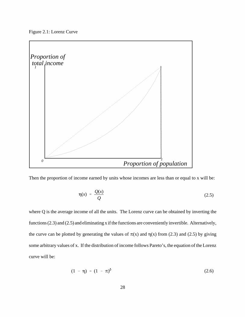
2.3.1 Lorenz Curve

The Lorenz curve is a powerful tool in the analysis of the size distribution of income and

wealth. The curve is defined as the relationship between the commutative portion of income and the

commutative portion of income receiving units. Let �(x) represent the proportion of the units that

receive income up to x and �(x) represent the proportion of total income received by the same units.

The Lorenz curve is then the graphical representation of the parametric relationship between � and

�. The graph of the curve is represented in a unit square. The straight line is joining the points (0,0)

and (1,1) is called the egalitarian line, because along the line � = �, which means that each unit

receives the same income. The Lorenz curve falls below the egalitarian line. Figure 2.1 illustrates

the Lorenz curve.

To derive the Lorenz curve, let x be the income of the unit and g(x) be the probability density

function of x. G(x)dx will then represent the probability that a unit selected at random will have

income less that or equal to x is:

and the average income earned by these units is:

28

0Proportion of population

Proportion of total income

1

1

�(x) �

Q(x)Q

(2.5)

(1 � �) � (1 � �)� (2.6)

Figure 2.1: Lorenz Curve

Then the proportion of income earned by units whose incomes are less than or equal to x will be:

where Q is the average income of all the units. The Lorenz curve can be obtained by inverting the

functions (2.3) and (2.5) and eliminating x if the functions are conveniently invertible. Alternatively,

the curve can be plotted by generating the values of �(x) and �(x) from (2.3) and (2.5) by giving

some arbitrary values of x. If the distribution of income follows Pareto’s, the equation of the Lorenz

curve will be:

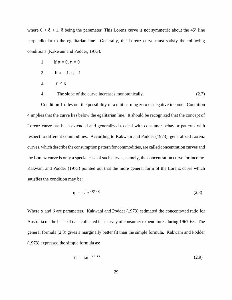
29

� � ��e��(1��) (2.8)

� � �e��(1��) (2.9)

where 0 < � < 1, � being the parameter. This Lorenz curve is not symmetric about the 450 line

perpendicular to the egalitarian line. Generally, the Lorenz curve must satisfy the following

conditions (Kakwani and Podder, 1973):

1. If � = 0, � = 0

2. If � = 1, � = 1

3. � < �

4. The slope of the curve increases monotonically. (2.7)

Condition 1 rules out the possibility of a unit earning zero or negative income. Condition

4 implies that the curve lies below the egalitarian line. It should be recognized that the concept of

Lorenz curve has been extended and generalized to deal with consumer behavior patterns with

respect to different commodities. According to Kakwani and Podder (1973), generalized Lorenz

curves, which describe the consumption pattern for commodities, are called concentration curves and

the Lorenz curve is only a special case of such curves, namely, the concentration curve for income.

Kakwani and Podder (1973) pointed out that the more general form of the Lorenz curve which

satisfies the condition may be:

Where � and � are parameters. Kakwani and Podder (1973) estimated the concentrated ratio for

Australia on the basis of data collected in a survey of consumer expenditures during 1967-68. The

general formula (2.8) gives a marginally better fit than the simple formula. Kakwani and Podder

(1973) expressed the simple formula as:

30

The standard error of the concentration ratio based on the general formula is higher than that of the

simple one. This may be because the concentration ratio is a function of a coefficient which could

not be estimated precisely in the general formula due to the high correlation between the independent

variables .

2.3.2 Gini Coefficient

The Gini coefficient is a well-known summary measure of inequality. It is derived from the

Lorenz curve. A variety of empirical studies on income distribution have used the Gini and extended

Gini to measure income distribution. Garner (1993) used the Lerman and Yitzhaki covariance

method to analyze inequality in the distribution of household consumption expenditures, and to

examine relationships between various expenditure budget components and total expenditures using

United States data. This method had been applied previously to the study income inequality by

income source in the U.S. (e.g., Ahearn, Johnson, and Strickland, 1985; Lerman and Yitzhaki,

1985), to assess the progressivity of taxation in Israel (Yitzhaki, 1990), and to determine the welfare

dominance of excise taxation for the Cote d’Ivoire (Yitzhaki and Thrisk, 1990).

Other researchers (e.g. Iyengar, 1960; Kakwani, 1978; Blaylock and Smallwood, 1982;

Yitzhaki, 1990; Yitzhaki and Thrisk, 1990) have used the Gini coefficient and concentration curves

to produce income or expenditure elasticities. In each of these previous studies, with the exception

of Kakwani (1978), elasticities were produced for a selected few commodities and commodity

groups.

Gartner’s (1993) study disaggregated total expenditures into nine exhaustive categories: food,

shelter, household fuels and utilities, household operations, apparel and services, transportation,

medical care and services, entertainment, and other expenditures. Expenditures allocated to savings,

31

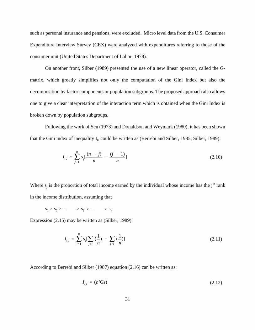
IG � �n

j�1sj[

(n � j)n

�

(j � 1)n

] (2.10)

IG � �n

i�1si[�

j�i

( 1n

) � �j�i

( 1n

)] (2.11)

IG � (e�Gs) (2.12)

such as personal insurance and pensions, were excluded. Micro level data from the U.S. Consumer

Expenditure Interview Survey (CEX) were analyzed with expenditures referring to those of the

consumer unit (United States Department of Labor, 1978).

On another front, Silber (1989) presented the use of a new linear operator, called the G-

matrix, which greatly simplifies not only the computation of the Gini Index but also the

decomposition by factor components or population subgroups. The proposed approach also allows

one to give a clear interpretation of the interaction term which is obtained when the Gini Index is

broken down by population subgroups.

Following the work of Sen (1973) and Donaldson and Weymark (1980), it has been shown

that the Gini index of inequality IG could be written as (Berrebi and Silber, 1985; Silber, 1989):

Where sj is the proportion of total income earned by the individual whose income has the jth rank

in the income distribution, assuming that

s1 � s2 � ... � sj � ... � sn

Expression (2.15) may be written as (Silber, 1989):

According to Berrebi and Silber (1987) equation (2.16) can be written as:

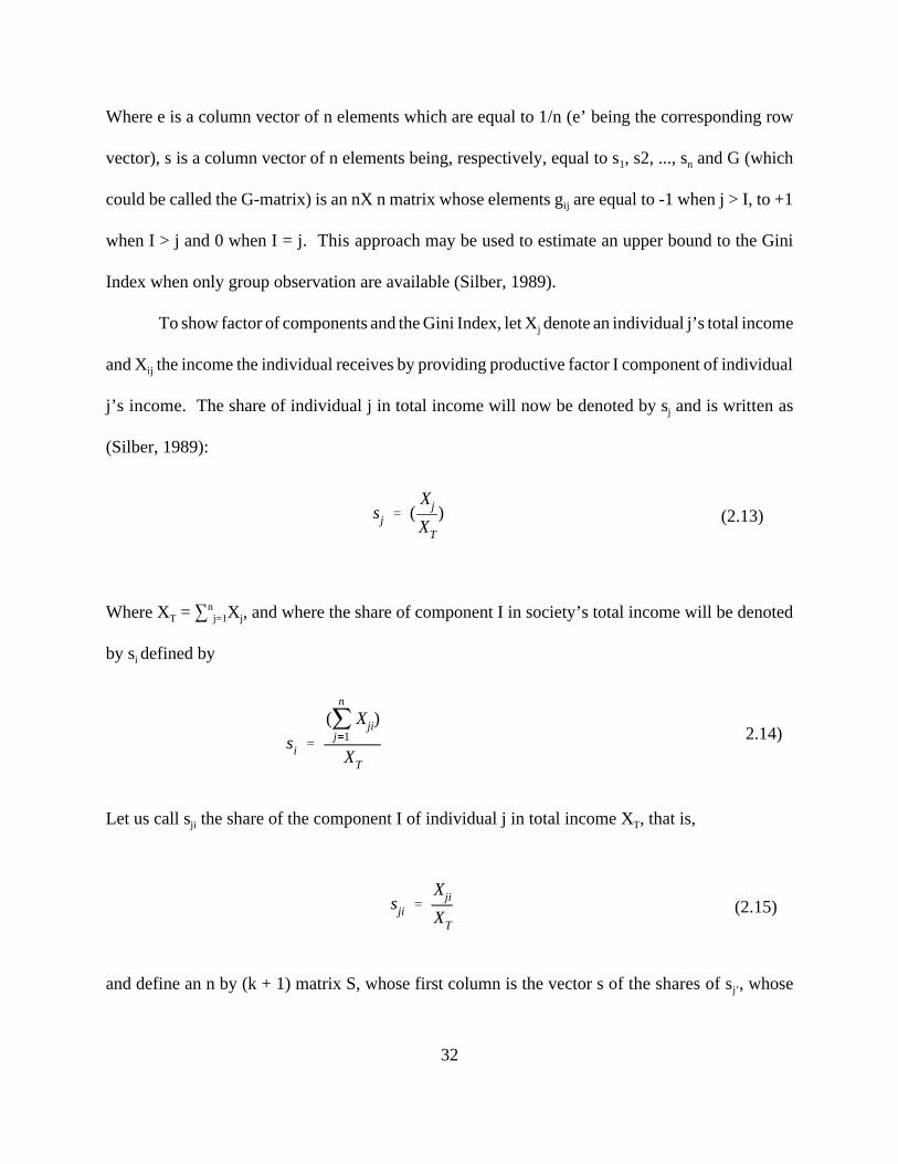
32

sj � (Xj

XT

) (2.13)

si �

(�n

j�1Xji)

XT

2.14)

sji �Xji

XT

(2.15)

Where e is a column vector of n elements which are equal to 1/n (e’ being the corresponding row

vector), s is a column vector of n elements being, respectively, equal to s1, s2, ..., sn and G (which

could be called the G-matrix) is an nX n matrix whose elements gij are equal to -1 when j > I, to +1

when I > j and 0 when I = j. This approach may be used to estimate an upper bound to the Gini

Index when only group observation are available (Silber, 1989).

To show factor of components and the Gini Index, let Xj denote an individual j’s total income

and Xij the income the individual receives by providing productive factor I component of individual

j’s income. The share of individual j in total income will now be denoted by sj and is written as

(Silber, 1989):

Where XT = �nj=1Xj, and where the share of component I in society’s total income will be denoted

by si defined by

Let us call sji the share of the component I of individual j in total income XT, that is,

and define an n by (k + 1) matrix S, whose first column is the vector s of the shares of sj’ , whose

33

e�GS � z (2.16)

zi�1 � e�Gs.i (i � 1...k) (2.17)

�k

i�1zi�1 � e�G(s.1 � ....� s.i � s.k)

� e�Gs � z1

(2.18)

zi�1 � e�G

(s1i

s.i

)s.i

.

.

.

(sni

s.i

)s.i

� zi�1 � e�Gv.i(s.i) � (s.i)e�Gv.i

(2.19)

second column is the vector s.1 of the shares sj1 and whose (I + 1)th column in the vector s.i of the

shares sji. The product

is a row vector of (k + 1) elements whose first element, as indicated by equation (2.12), is the Gini

Index of total income inequality. The next k element of z may be written as:

so that

Let us call v.i the vector of the ratios (sji/s.i) (j = 1...n) so that the element vji of v.i is the share of

individual j in the total income derived from component I. Expression (2.17) may then be written

as:

34

Gi � e�Gy.i (2.20)

The scalar e’Gv.i is generally not the Gini Inequality Index Gi of the ith component of income since

the elements vji and v.i (j = 1....n) may not necessarily be ranked by decreasing value as are the

elements sj. of s. To obtain the Gini Inequality index of Gi of component I, one has to construct a

new vector y.i whose elements yji (j = 1.....n) are the shares (sji/s.i) previously defined, but they are

not ordered according to the order of the shares sj of vector s but according to their own rank in the

vector y.i. The Gini Index Gi for component I is therefore defined as:

The scalar Ci = e’Gv.i, on the other hand, has been called the pseudo Gini of component I by Fei,

Ranis and Kuo (1978) or the concentration ratio of component I by Rao (1969), Kakwani (1980),

Pyatt, Chen and Fei (1980) and Shalit (1985).

The above procedure to decompose the Gini Inequality Index among all factors that

contribute to income is, therefore, relatively uncomplicated. It requires construction of a matrix S

whose first column refers to the shares of each individual’s total income in society’s total income

whereas the next column refers to the shares of each individual’s income from specific component

in society’s total income (Silber, 1989). All vectors are ranked according to the (decreasing) rank

of the individuals in total income. The product e’GS is then a vector z whose first element is the

Gini Inequality Index IG, whereas the other elements are the contributions of each component to the

overall inequality IG. Both techniques presented above were tested with real data. The outcome is

very consistent with the other measures of inequality.

Another study, by Husted (1991), examines the change in state-level income inequality from

1981 to 1987. Inequality is measured by the state’s Gini coefficient, as calculated from each state’s

35

P(Y) � �y

0f(Y)dY (2.21)

Q(Y) �

1µ �

y

0Y f(Y) dY (2.22)

� �

1

2[P(Y) � Q(Y)], � �

1

2[P(Y) � Q(Y)] (2.23)

d�d�

�

(µ � y)(µ � y)

(2.24)

Lorenz curve. The study uses techniques developed in Kakwani and Podder (1973, 1976) and

described in Slottje (1989) to estimate state-leve Lorenz curves. The parameter estimates then are

used to calculate the associated Gini coefficients and their asymptotic standard errors.

Following Kakwani and Podder (1976), family income Y is a random variable with

probability density function f(Y), so that

is the proportion of families with income less than or equal to y and

is the proportion of income earned by the families who have income less than or equal to y, where

µ represents the mean income of all families in the population.

Given these definitions, any point of a Lorenz curve can be described by two line segments,

The first line segment � is the ordinate from the point on the Lorenz curve to the diagonal egalitarian

line. The second segment (�) extends from the origin to this ordinate along the diagonal egalitarian

line. It follows this definition that

The proposed Lorenz curve for this study is (Husted, 1991):

36

� � a� � ( 2 � �)�,0 < � < 2, �: a, �, � > 0 (2.25)

log(�) � log(a) � � log (�) � � log ( 2 � �) (2.26)

�( 2 � �) � �� �

(µ � y)(µ � )

�( 2 � �)

�(2.27)

Taking the log of both sides, equation (2.25) becomes

This specification satisfies the necessary properties for a Lorenz curve (Husted, 1991). In particular,

� > 0 when a > 0 and the Lorenz curve lies below the egalitarian line. The parameters � and � are

restricted to be greater than zero, so that � = 0 when � = 0 or � = �2. Additional restrictions are

imposed by equation (2.24) and the negative second derivative. The additional restrictions contain

0 < � � 1 and 0 < � � 1 and indicate, for the Lorenz curve defined in equation (2.25), that

To calculate the Gini coefficient, the parameters of the Lorenz curve in equation (2.25) and the

restriction on the curve in equation (2.26) must be jointly estimated. However, since the available

income data for the analysis by Husted (1991) are grouped by income class, � and � are not observed

(Husted, 1991). In the data used for this study, there are N families grouped into K + 1 income

classes for each time series t (1 = 1,.......,T) and within each cross section. If nt,ck is the number of

families earning income between yk-1 and yk in time period t and cross section c, then ft,ck = nt,c

k/N

is a consistent estimator of the probability that a family belongs to this particular income group in

cross section c and time t (Husted, 1991). Therefore the estimators of P(Y) and Q(Y) are (Husted,

1991):

37

p kt,c � �

k

f��1�

t � 1,.....C

q kt,c �

1µt,c

�k

��1m�f�

t � 1,..........,T. c � 1,.........C.(2.28)

I kt,c �

[p kt,c � q k

t,c]

2, n k

t,c �

[p kt,c � q k

t,c]

2(2.29)

log (n kt,c � a �

� � log (I kt,c) � � log ( 2 � I k

t,c) � 1 (2.30)

(µt,c � yk)

(µt,c � yk)

( 2 I kt,c)

n kt,c

� � ( 2 � I kt,c) � � (I k

t,c) � 1 (2.31)

where m� is the mean income group �, and µt,c is the mean income for all families in cross section

c and in year t. By substituting pt,ck and qt,c

k into the expressions in equation (2.23), consistent

estimators of � and � are (Husted, 1991):

Since the estimators differ from the true � and � by a random disturbance, equation (2.26) is

expressed as:

Finally, after substituting pt,ck and qt,c

k for � and �, equation (2.27) becomes

A joint generalized least square (GLS) estimation of the proposed Lorenz curve in the equation

(2.30) and its restrictions in equation (2.31) is carried out for state level grouped pre-tax family

income data (Husted, 1991). This estimation is more efficient than ordinary least squares estimation

38

G � 2a ( 2)1 �� �� � (1 � �, 1 � �) (2.32)

of the Lorenz curve parameters in equation (2.29). With the estimated coefficients from the GLS

estimation - a, �, and �, the Gini coefficient can be calculated. The Gini coefficient for each state

derived from the Lorenz curve in equation (2.29) is (Husted, 1991):

where � (1 + �, 1 + �) is the beta function, with 1 + � and 1 + � degrees of freedom.

The calculated state level Gini coefficients for family income from 1981 to 1987 reflect the

increasing inequality observed in the United States during the 1980s (Husted, 1991). This measure

also indicates significant differences in the growth of family income inequality across states.

Although the paper did not explore the exact cause of these differences, they reflect, in part, the

uneven incidence of the state level economic restructuring, from high and middle wage

manufacturing, construction, and mining sectors to the low wage service and trade sectors (Husted,

1991).

To explain the drawbacks to Gini measurements, Braun (1988) re-examined the direct

relationship between income inequality (as measured by a variety of indices, including the Gini ratio)

and development or economic improvement (as measured by several independent variables,

including mean income). A corollary hypothesis suggested by Braun is that the original

relationships may not be present when other measurements of income inequality are employed, both

because of their differing sensitivities and because these alternate techniques are measuring

substantively different types of income inequality. Growing evidence shows that the Gini ratio has

serious weaknesses (Braun, 1988). The simple aging of a population will increase inequality

(Morgan, 1962). Although Paglin (1975) introduced a modification to correct for this bias, it has

39

not been widely adopted in subsequent research. A popular method of computing Gini scores

utilizes census income categories, frequently with the adjustment using a Pareto curve for the open-

ended interval at the top (Knott, 1970). Employing the Pareto curve is not always done, however,

which can lead to inconsistent comparisons. It has been shown that the Gini coefficient will be

reduced to the degree that the number of income intervals also declines (Sale, 1974). Income

intervals differ from one census to another, with 14 in 1950, 13 in 1960, 15 in 1970, and 9 in 1980.

The Gini coefficient is also insensitive to non-money income components and differential

price indices between states, which exaggerate income inequalities in rural area (Jonish and Kau,

1973). Bud (1973) finds a tendency toward error for researchers making comparisons between

various dates. Additionally, the Gini coefficient is more responsive to changes in income of the

middle class than to changes among the rich or the poor (Osberg, 1984; Allison, 1978). This is

perhaps why Gini scores show such stability over long periods of time in the United States (Braun,

1987). One study of Wisconsin income data (Soltow, 1971) shows no great change in Gini scores

over 100 years. Reynolds and Smolensky (1977) find that despite major changes in taxation and

welfare in the 1950-1970 period, inequality is virtually unchanged as measured by Gini ratios. A

serious problem also results when Lorenz curves intersect as countries are compared (Allison, 1978).

Schwarz and Winship’s (1979) re-examination of Kuznets’ data concludes that of 66 possible pairs

of comparisons between countries, in only 16 comparisons is it possible to use Lorenz-based Gini

scores to discover which country unequivocally has the most unequal distribution of income (Braun,

1988).

2.3.3 Stochastic Dominance

Until relatively recently, the conventional view in economics was that the size distribution

40

W � � U(x) dF � � U(x) dF�(33)

of income does not change very much across time (Bishop and Formby, 1994). Dominance

techniques for ranking entire distributions stand at the forefront of these developments. If two

income distributions differ, which one is better? If two growth processes distribute the benefits of

economic growth differently, which is better? The dominance method can be used to address both

of this questions. If we are interested in comparing two multi-variance distributions, represented by

the (continuous) cumulative distribution functions F(x) and F*(x), where x is a vector of random

variables. It is assumed that the comparison is based on the difference in expected utility (Atkinson,

1983):

Where expected utility is assumed to be well-defined. One distribution, F, is said to stochastically

dominate the other, F*, for a specific class of utility functions when W is non-negative for all U�U

and is strictly positive for some U (Atkinson, 1983). The condition for F to dominate F* becomes

progressively weaker as one strengthens the conditions on the class U .

The dominance method of evaluating income distributions is very general and can be applied

to investigate income inequality, economic efficiency, and changes in the overall status of welfare

in an economic system. It can also be applied to evaluate the distribution of the benefits of economic

growth across time. Recent empirical studies based on the dominance principle are indicative of the

applicability of the methodology to the study of statistical distributions in general. Examples where

dominance methodology is used to evaluate a variety of issues are changes in the U.S. income

distribution across time (Bishop, Formby and Smith, 1991a; Bishop, Chow and Formby, 1991a); the

convergence and divergence of U.S. regional income distribution in the 1970s (Bishop, Formby and

41

Thistle, 1992a,b); the effects of growth and recessions on poverty (Bishop, Chow and Formby,

1991a); international differences in income distribution (Bishop, Formby and Smith, 1991b, 1993;

Bishop, Formby and Sakano, 1992a); the effects of tax evasion on the distribution of income and tax

burdens (Bishop ,Chow and Formby, 1991b; Bishop, Chow, Formby, and Ho, 1993); the effects of

the U.S. Food Stamp program on under nutrition (Bishop, Formby and Zeager, 1992b); and

differences in mortality distributions and the problem of "missing women" in major regions of the

LDC world (Bishop, Formby and Zeager, 1992a).

According to Bishop and Formby (1994), the appeal of the dominance approach is traceable

to three distinct but related features of the methodology. First, it rests upon explicit welfare criteria

that are widely acceptable and which rank the distributions of interest using a series of steps, or

stages, that are referred to as first, second, and third degree dominance. If two distributions can be

ranked, any two researchers or policy makers are likely to be in general agreement concerning which

of the distributions is best. Second, new statistical inference procedures developed over the last

decade have substantially expanded the capacity of the dominance method to rank income

distributions and evaluate comparative levels of welfare. As a consequence, studies of income

distribution need no longer rely on descriptive statistics, but can make use of explicit tests of

hypothesis. The dominance method relies on ordinal measures of entire distributions and levels of

welfare, while avoiding the use of index numbers that rest on a dubious assumption of cardinality.

If two income distributions differ, which is "better"? If two growth processes distribute the

benefits of economic growth differently, which is better? The dominance method can be used to

answer both of these questions. Important theoretical contributions by Atkinson (1970), Shorrocks

(1983), and Saposnick (1981, 1983) establish a powerful relationship between the dominance of one

42

income distribution over another and ordinal level of welfare. Foster and Skorrocks (1988) extend

the theory to show an equally powerful relation between dominance of income distribution and

poverty. New statistical inference procedures pioneered by Beach and Davidson (1983) complement

the theoretical developments by permitting the dominance relationship between income distributions

to be subjected to rigorous hypothesis testing.

Atkinson (1970) demonstrates that, for distributions with equal means, strong inferences can

be made about comparative states of economic welfare when one Lorenz curve dominates another.

As emphasized by Sen (1973), when the mean of the distributions of interest are unequal, the Lorenz

dominance principle is devoid of welfare content. In related but distinct ways, Shorrocks (1983) and

Saposnik (1981, 1983) extended the dominance approach to consider distributions with unequal

means. Shorrocks demonstrates that Lorenz curves can be re-scaled by the mean of the distribution

and dominance comparison can be made in the same fashion as with ordinary Lorenz curves.

Shorrocks refers to this re-scaled Lorenz curve as the Generalized Lorenz curve. Like dominance

in terms of ordinary Lorenz, GL dominance incorporates a preference for equality; but unlike the

Lorenz curve, the GL curve also incorporates an efficiency preference (Bishop and Formby, 1994).

Saposnik (1981, 1983) adopts a more straightforward approach and applies first order dominance

techniques directly to income distributions. The criterion compares absolute income in ranked

positions in the income distribution and is referred as "rank dominance" (Bishop and Formby, 1994).

It is well established that first order dominance implies second order dominance; as a result rank

dominance implies GL dominance. Further, a first order dominance is a pure efficiency criterion

and, unlike second order dominance, does not contain a preference for equity (Bishop, Formby and

Smith, 1991a)

43

Several sources of micro data have been analyzed and some of the findings from the analysis

of CPS, Public Use Samples of the decennial Census of Populations are summarized below. The

Internal Revenue Service’s Tax payer Compliance Measurement Program (TCMP) and the

Luxembourg Income Study are two such studies. Perhaps the most dramatic change uncovered using

inferences based dominance analysis is the rise in U.S. income inequality in the period following

1978. Bishop, Formby and Smith (1991a) analyze the period 1967-1986 and present statistics that

identify the sub-periods: 1967-1977, 1978-1982 and 1983-1986. Their results reveal a significant

rise in inequality between 1978 and 1982 which they describe as "massive". Before 1978, there were

several statistically significant changes in U.S. Lorenz curves, which were associated with cyclical

swings in the economy (Bishop and Formby, 1994). Consistent with earlier findings of Beach

(1977) and Blinder and Esaki (1978), inequality rose in recession years and declined in years of

recovery. But beginning 1978, the shifts in Lorenz curves were different; inequality began to rise

well before any recession, the changes were quite large by historical standards, and there were no

reverse movements toward equality during the period of recovery (Bishop, Formby and Smith,

1991a). In fact, inequality rose slightly between 1982 and 1986. Further, a more recent study

(Bishop, Chiou and Formby, 1992) extends the Lorenz dominance analysis to 1989 and finds that

inequality continued to rise in the late 1980s.

The second dramatic change in U.S. income distributions revealed by inference-based

dominance analysis involves convergence of regional income distributions in the 1970s (Bishop,

Formby and Thistle, 1992a,b). The U.S. south historically had both lower absolute incomes and

greater inequality than the Non-South. Bishop, Formby and Thistle (1992a) apply the dominance

methodology to Public Use Samples from the 1970 and 1980 decennial censuses and show that, as

44

expected, the South was unambiguously dominated in 1969. However, the evidence reveals

extraordinary changes in the 1970s. Lorenz curves, first order dominance and second order

dominance all indicate that the south’s income distribution either converged or almost converged

to that of the Non-South (Bishop and Formby, 1994).

The third dramatic result from inference-based dominance analysis comes from a follow-up

study of U.S. regional income distribution. Bishop, Formby and Thistle (1992b) disaggregate the

Non-South into its major sub-regions consisting of the West, Midwest, and Northeast and apply the

same methodology used to show the convergence of the South to Non-South. Income distributions

in the major regions of the Non-South were equivalent in 1969 and the South was uniformly

dominated by all other regions. Bishop and Formby (1994) further point out that fundamental

changes in the 1970s resulted in the West’s rank dominating the Midwest, which dominated the

South, which in turn dominated the Northeast. Thus, while the South’s income distribution was

converging to the Non-South, the West, Northeast and Midwest income distributions were

significantly diverging from one another (Bishop, Formby and Thistle, 1992a,b).

The fourth dramatic result uncovered using inference-based dominance analysis relates to

the effects of tax evasion on the U.S. distribution of income and tax burdens. Bishop, Chow and

Formby (1991b) and Bishop, Chow, Formby, and Ho (1993) use the internal revenue service TCMP

micro data to analyze the effects of tax evasion on the Lorenz and associated concentration curves

of income and tax burdens. Confidential TCMP data consisting of weighted samples of

approximately 50,000 tax payers were analyzed for 1979, 1982, and 1985 Bishop, Chow and

Formby,1991b; Bishop, Chow, Formby, and Ho, 1993). According to Bishop, Chow and Formby

(1991b); Bishop, Chow, Formby and HO (1993) the results reveal a surprising but consistent

45

pattern; lower income tax-paying units under report a larger percentage of their incomes than higher

income tax-paying units and pay proportionally less tax than required under the Internal Revenue

Code (IRC). Stated differently, higher income receiving units have smaller shares of after-tax

income and pay larger shares of the income tax burden before the TCMP audits than they do after

random audits and compulsory compliance with the IRS (Bishop, Chow and Formby,1991b; Bishop,

Chow, Formby, and Ho, 1993).

The dominance technique is a general method that can be applied to evaluate income

inequality, economic efficiency, and changes in the overall level of welfare in an economic system.

This methodology has been used by many economists to address a variety of issues related to

income, welfare and economics in general. The dominance technique remains one of the widely

used methodologies.

2.3.4 An Income-Net Worth Approach

The income - net worth measure is based on the assumption that current income and current

net worth are both important determinants, although not the sole determinants, of the economic

position of a consumer. An individual’s economic well-being should be thought of as a function of

the flow of services over which he or she has command. This flow depends importantly on the

consumer’s current income and also on the services received from his or her assets, net of liabilities

(Moon, 1977; Weisbrod and Hansen, 1977).

Weisbrod and Hansen used data from the Survey of Financial Characteristics of Consumers

(SFCC) and the Current Population Survey (CPS) for 1962 to measure well-being or economic

inequality in the United States. The SFCC provides data on families by age of head, income, and

net worth; the CPS provides data on family income by age of head, broken down into finer income

46

classes. As Weisbrod and Hansen pointed out, the income-net worth approach while incomplete as

a measure of economic welfare, has a number of useful attributes, the major one being that of

merging two separate but obviously related measures of economic status into a unified measure. The

most striking result is its impact on the economic position of the aged, who by this measure appear

to be considerably better-off than is shown by the current income measure (Weisbrod and Hansen,

1977). This results from the interaction of income, net worth holdings, and life expectancy. The

authors suggest that the income-net worth measure may be useful as a basis for redefining tax

progressivity, and as explanatory variable in consumption behavior theory.

An empirical study by Moon (1977) also used the income-net worth approach to measure the

economic well-being of the aged poor. To derive an empirical approximation of the potential

consumption measure, she makes several adjustments to the annual money income indicator of

economic status. These adjustments include an imputation for net worth including home equity, the

addition of an estimate of the cash value of three in-kind transfers -- medicare, medicaid, and public

housing -- the subtraction of an estimate of income and payroll taxes paid and the addition of an

estimate of intra-family transfers. Moon then examines how the rankings of several groups of the

aged vary with the definition of economic status that she employs. She discovers, for example, that

relative to the annual money income measure, her more comprehensive measure of economic status

places an even larger proportion of families headed by nonwhites in the bottom part of the

distribution of economic well-being. An unexpected finding is that more aged families with workers

fall into the bottom part of the distribution when the more comprehensive measure of economic

status is used.

Finally, Moon employs her more comprehensive definition of economic well-being to

47

examine the impact of government programs on the well-being of the aged. Five cash transfer

programs are examined: social security, public assistance, government pensions, veterans’ benefits,

unemployment insurance, and workmen’s compensation; also included are three in-kind transfer

programs (medicare, medicaid, and public housing) and three income tax provisions (the double

personal exemption, exclusion of transfer income, and the retirement tax credit). Moon discovered

that government pensions, workmen’s compensation, and unemployment benefits do provide

substantial benefits to some aged families. Social security and medicare provide almost universal

coverage for the aged but are a very inefficient way of helping those at the lower end of both

distributions. The study also revealed that the income-conditioned transfers which provide the

greatest share of benefits to aged families with the lowest resource level are none-the-less of limited

help to this group. On the tax expenditure Moon writes that it is the most inefficient means for

directing resources towards the aged poor.

In addition to the above methods of measuring income distribution, there are numerous other

ways of measuring inequality. A large number of books and articles have articulated this issue to

the point of saturation. What is being questioned is the level of precision of these studies and their

methodological approach. The need for the development of a better approach to measure the well-

beingness of families has become a hot topic in welfare economics.

2.4 The Contributions of this Research

The empirical results from this research will be used as indicators of economic well-being

and will provide a better understanding for formulating public policy. The results are also expected

to shed light on the impacts of relative price changes and the impacts of household composition on

the patterns of distribution of household consumption expenditures. An examination of inequality

48

at a desegregated level will reveal that most of the level and trends of the consumption-based

measure can be explained by within group movements rather than inequality between groups. This

is true for households expenditures classified by commodity components, age, and race. A greater

effort will be devoted in summarizing the results and rationalizing the implications.

The theoretical and empirical background included in this study will definitely consolidate

and expand the dimension of the literature (knowledge) concerning this topic and the issue of welfare

measurement in general. The use of combined time series and cross sectional data may reveal some

interesting results in the measurement of the impact of demographic attributes on the distribution

of consumption expenditures. This is a major contribution expected from of this research. The

empirical results of this study should also enable comparison of the inequality in the distribution of

consumption expenditure among the years between 1980 and 1994.

49

CHAPTER 3: THEORETICAL FRAMEWORK

3.1 Introduction

This chapter addresses the conceptual and methodological framework based on a remarkable

convergence that has occurred between economic theory and econometrics over the past decade

(Jorgensen et al., 1982). This convergence has taken place between the theory of social choice and

econometric modeling of aggregate consumer behavior. The result of this phenomenon has produced

a new approach to normative economics. This new approach has been implemented to test and

evaluate economic policies, measure poverty and inequality, and assess the standard of living and

its cost.

The following sections will be presented in this chapter: In section 3.2 aggregate consumer

behavior is derived based on the theory of exact aggregation, following Jorgensen (1980, 1981, 1982,

1984); conclusions and a summary of the theoretical framework are given in section 3.3; section 3.4

presents methods for examining inequality in the distribution of consumption expenditures.

3.2 Aggregate Consumer Behavior

According to Jorgensen et al. (1982), a common problem in modeling consumer behavior

and social choice is the representation of individual preferences. Simplification of the aggregate

demand function is necessary for econometric modeling of aggregate consumer behavior. The

simplest and most familiar approach to this problem is the technique of a representative consumer

(Jorgensen et al., 1982). This model is required to justify applications of the theory of individual

consumer behavior to aggregate data on prices and quantities consumed. The model is based on the

assumption of identical homothetic preferences for all individuals.

Under identical homothetic preferences, aggregate quantities consumed are functions of

50

aggregate expenditure and prices. The functions exhibit the same properties as demand functions

in the theory of individual consumer behavior. The conditions for identical homothetic preferences

was weakened by Gorman (1953) to permit displacements from the origin. Gorman showed that a

necessary and sufficient condition for aggregate demand functions to depend on aggregate

expenditure is that all individuals must have parallel linear Engle curves. This condition has been

used many times in modeling aggregate consumer behavior.

In 1975, Muelbauer significantly broadened Gorman’s definition of the concept of a

representative consumer and constructed a model of a representative consumer where individual

preferences are assumed to be identical, but not necessarily homothetic. Aggregate expenditure

shares depend on prices and a function of the distribution of individual expenditures that is not

restricted to aggregate expenditures. A model developed by Lau (1977b), however, does not require

the concept of a representative consumer. Aggregate demand functions are obtained by exact

aggregation over individual demand functions. The model incorporates differences in individual

preferences into demand functions through attributes of individuals such as demographic

characteristics. Aggregate demand functions depend on the joint distribution of attributes and total

expenditure over all consuming units through summary statistics of the distribution. Jorgensen et

al., (1982) point out that within the framework provided by Lau (1977b) and Muellbauer (1975), the

assumption of identical homothetic preferences for all individuals appears as a highly over-

simplified approach to modeling aggregate consumer behavior. Homethetic preferences are

inconsistent with well established empirical regularities in the behavior of individual consumers

(Jorgensen and Slesnick, 1984). Besides, identical preferences are inconsistent with empirical

findings that expenditure patterns depend on the demographic characteristics of consumers, among

51

other factors.

This framework to the measurement of welfare inequality is based on the an econometric

model of aggregate consumer behavior. The advantage of this approach is that systems of individual

demand functions can be obtained from the system of aggregate demand functions. Based on that

demand function being integrable, one can recover the indirect utility functions for all consumers.

Measures of individual welfare can be defined in terms of these utility functions.

To represent preferences for all individuals in a form suitable for measuring individual

welfare, households are taken as a consuming unit. It is assumed that expenditures on individual

commodities are allocated so as to maximize a household’s welfare function. As a consequence, the

household behaves in the same way as an individual maximizing a utility function, as demonstrated

by Samuelson (1956) and Pollak (1981). By assuming that each household maximizes a household

welfare function, the focus can be on the distribution of welfare among households rather than the

distribution among individuals within households.

To construct an econometric model based on exact aggregation, individual preferences are

represented by means of an indirect utility function for each consuming unit, using the following

notation (Jorgenson and Slesnick, 1984):

pn is the price of the nth commodity, assumed to be the same for all consuming units.

p = (p1, p2,....., pN) is the vector of prices of all commodities,

xnk is the quantity of the nth commodity group consumed by the kth consuming unit

(n= 1,2,......., N; k = 1, 2,........, K),

Mk = �n=1 N pnxnk to the total expenditure of the kth consuming unit (k = 1, 2,,......, K),

wnk = pnxnk/Mk is the expenditure share of the nth commodity group in the budget of the kth

52

ln pMk

� (lnp1

Mk

, lnp2

Mk

,........, lnpN

Mk

), 3.1

ln Vk � G(lnp �

Mk

�p �

12

lnp �

Mk

�pp lnp �

Mk

�paAk, Ak)

(k�1,2,....,K)(3.2)

lnp �

Mk

�p �

12

lnp �

Mk

�pp lnp

Mk

� lnp �

Mk

�pAAk (3.3)

consuming unit (n = 1, 2,......., N; k = 1, 2,........., K),

wk = (w1k, w2k,........, wNk) is the vector of expenditure shares for the kth consuming

unit, (k =1, 2,......., K),

is the vector of logarithms of ratios of prices to expenditure by the kth consuming unit (k =

1,2,.....,K),

ln p = (ln p1, ln p2,......, ln pN) is the vector of logarithms of prices, and

Ak is the vector of attributes of the kth unit (k = 1, 2,....., K).

It is assumed that the kth consuming unit allocates expenditures in accord with the transcendental

logarithmic or translog indirect utility function, say Vk, where:

In this representation, the function G is a monotone increasing function of the variable:

In addition, the function G depends directly on the attribute vector Ak. The vector �p and the

matrices �pp and �pA are constant parameters that are the same for all consuming units.

The expenditure shares of the kth consuming unit can be derived by the logarithmic form of

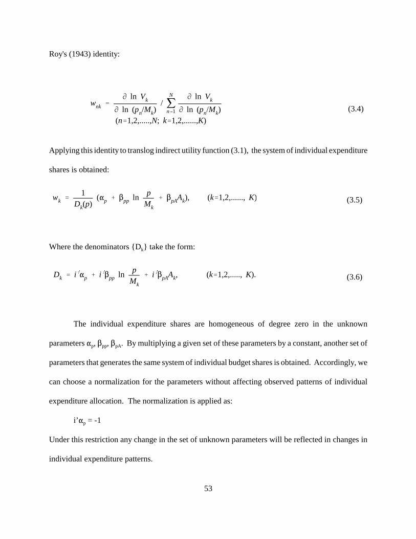
53

wnk �

� ln Vk

� ln (pn/Mk)/ �

N

n�1

� ln Vk

� ln (pn/Mk)(n�1,2,.....,N; k�1,2,......,K)

(3.4)

wk �

1Dk(p)

(�p � �pp lnp

Mk

� �pAAk), (k�1,2,......,K) (3.5)

Dk � i ��p � i ��pp lnp

Mk

� i ��pAAk, (k�1,2,.....,K). (3.6)

Roy's (1943) identity:

Applying this identity to translog indirect utility function (3.1), the system of individual expenditure

shares is obtained:

Where the denominators {Dk} take the form:

The individual expenditure shares are homogeneous of degree zero in the unknown

parameters �p, �pp, �pA. By multiplying a given set of these parameters by a constant, another set of

parameters that generates the same system of individual budget shares is obtained. Accordingly, we

can choose a normalization for the parameters without affecting observed patterns of individual

expenditure allocation. The normalization is applied as:

i’�p = -1

Under this restriction any change in the set of unknown parameters will be reflected in changes in

individual expenditure patterns.

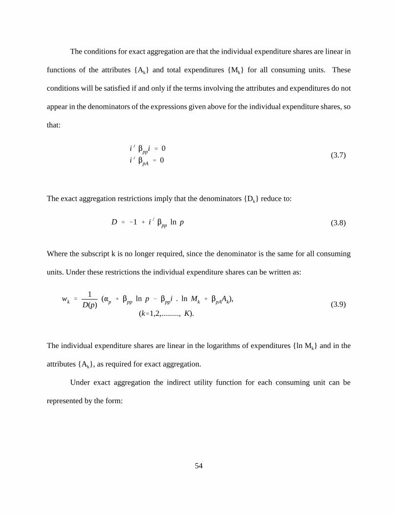
54

i � �ppi � 0

i � �pA � 0(3.7)

D � �1 � i � �pp ln p (3.8)

wk �

1D(p)

(�p � �pp ln p � �ppi . ln Mk � �pAAk),

(k�1,2,.........,K).(3.9)

The conditions for exact aggregation are that the individual expenditure shares are linear in

functions of the attributes {Ak} and total expenditures {Mk} for all consuming units. These

conditions will be satisfied if and only if the terms involving the attributes and expenditures do not

appear in the denominators of the expressions given above for the individual expenditure shares, so

that:

The exact aggregation restrictions imply that the denominators {Dk} reduce to:

Where the subscript k is no longer required, since the denominator is the same for all consuming

units. Under these restrictions the individual expenditure shares can be written as:

The individual expenditure shares are linear in the logarithms of expenditures {ln Mk} and in the

attributes {Ak}, as required for exact aggregation.

Under exact aggregation the indirect utility function for each consuming unit can be

represented by the form:

55

ln Vk�F(Ak)� ln p �(�p�12

�pp ln p � �pAAk) � D(p) ln Mk,

(k � 1,2,......................,K).(3.10)

Uk � U[x1k

m1(Ak),

x2k

m2(Ak),.......,

xNk

mN(Ak)],

(k�1,2,...............,K),

(3.11)

Mk � �N

n�1pnxnk, (k�1,2,.......,K), (3.12)

In this representation the indirect utility function is linear in the logarithm of total expenditures (ln

Mk) with a coefficient that depends on the prices p(k=1,2,........, K). This property is invariant with

respect to positive affine transformations, but is not preserved by arbitrary monotone increasing

transformations. It is concluded that the indirect utility function (3.10) provides a cardinal measure

of utility for each consuming unit.

To provide a basis for evaluating the impact of transfers among households on social welfare,

it is useful to represent household preferences by means of a utility function that is the same for all

accounting units. For this purpose, it is assumed that the kth consuming unit maximizes its utility,

say Uk, where:

subject to the budget constraint

In this representation of consumer preferences, the quantities {xnk/mn(Ak)} can be regarded as

effective quantities consumed, as proposed by Barten (1964). The crucial assumption embodied in

this representation is that differences in preferences among consumers enter the utility function U

56

Vk � V[p1m1(Ak)

Mk

,p2m2(Ak)

Mk

,.........,pNmN(Ak)

Mk

],

(k�1,2,..................,K).

(3.13)

only through differences in the commodity specific household equivalence scales {mk(Ak)}.

Consumer equilibrium implies the existence of an indirect utility function, say V, that is the

same for all consuming units. The level of utility for the kth consuming unit, say Vk, depends on the

prices of individual commodities, the household equivalence scales, and the level of total

expenditure:

In this representation the prices {pn mn(Ak)} can be regarded as effective prices. Differences in

preferences among consuming units enter this indirect utility function only through the household

equivalence scales {mn(Ak)} (k=1,2,..........., ).

To represent the translog indirect utility function (3.2) in terms of household equivalence

scales, Jorgenson and Slesnick (1984) used some additional notations:

ln pm(Ak)/Mk is the vector of logarithms of ratios of effective prices {pnmn(Ak)} to total

expenditure Mk of the kth consuming unit (k=1,2,......, K), and

ln m(Ak) = (ln m1(Ak), ln m2(Ak),..........., ln mN(Ak) is the vector of logarithms of the

household equivalence scales of the kth consuming unit (k=1,2,........., K).

It is assumed, as before, that the kth consuming unit allocates its expenditures in accord with

the translog indirect utility function (3.2). However, it is assumed that this function, expressed in

terms of the effective prices {pnmn(Ak)} and total expenditures Mk, is the same for all consuming

units. The indirect utility function takes the form:

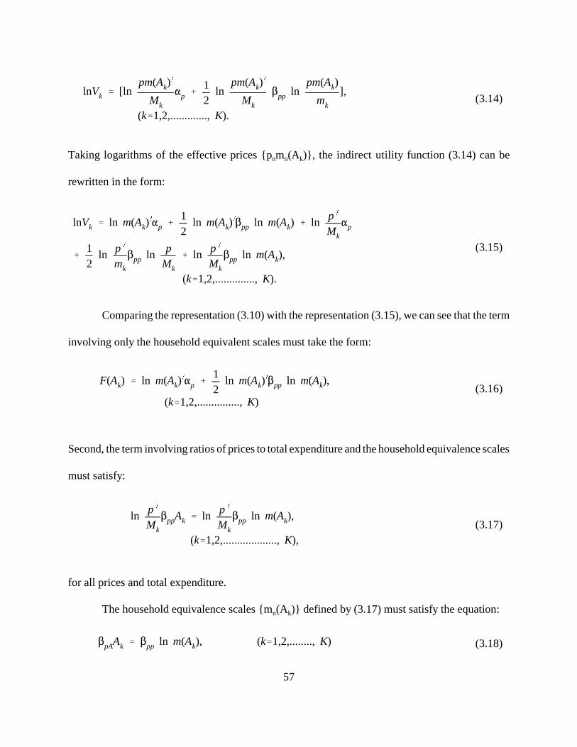
57

lnVk � [lnpm(Ak)

�

Mk

�p �

12

lnpm(Ak)

�

Mk

�pp lnpm(Ak)

mk

],

(k�1,2,.............,K).

(3.14)

lnVk � ln m(Ak)��p �

12

ln m(Ak)��pp ln m(Ak) � ln

p �

Mk

�p

�

12

lnp �

mk

�pp lnp

Mk

� lnp �

Mk

�pp ln m(Ak),

(k�1,2,..............,K).

(3.15)

F(Ak) � ln m(Ak)��p �

12

ln m(Ak)��pp ln m(Ak),

(k�1,2,...............,K)(3.16)

lnp �

Mk

�ppAk � lnp �

Mk

�pp ln m(Ak),

(k�1,2,...................,K),(3.17)

�pAAk � �pp ln m(Ak), (k�1,2,........,K) (3.18)

Taking logarithms of the effective prices {pnmn(Ak)}, the indirect utility function (3.14) can be

rewritten in the form:

Comparing the representation (3.10) with the representation (3.15), we can see that the term

involving only the household equivalent scales must take the form:

Second, the term involving ratios of prices to total expenditure and the household equivalence scales

must satisfy:

for all prices and total expenditure.

The household equivalence scales {mn(Ak)} defined by (3.17) must satisfy the equation:

58

ln m(Ak) � ��1pp�pAAk, (k�1,2,.........,K). (3.19)

ln Vk � A /k�

/pA�

�1pp�p �

12

A /k�pA�

�1pp�pAAk � ln p �(�p

�

12�pp ln p � �pAAk) � D(p) ln Mk,

(k�1,2,........................,K).

(3.20)

ln Mk �

1D(p)

[A /k�

/pA�

�1pp�p �

12

A /k�pA/�pp�1�pAAk

� ln p �(�p �

12�pp ln p � �pAAk) � ln Vk],

(k�1,2,......................,K).

(3.21)

Under monotonicity of the individual expenditures shares the matrix �pp has an inverse, so that we

can express the household equivalence scales in terms of the parameters of the translog indirect

utility function, �pp, �pA , and the attributes {Ak}:

These scales are referred to as the commodity specific translog household equivalence scales.

Substituting the commodity specific equivalence scales (3.18) into the indirect utility function

(3.15) a representation of the indirect utility function can be obtained in terms of the attributes {Ak}:

This form of the translog indirect utility function is equivalent to the form (3.2) in that both generate

the same system of individual demand functions. By requiring that the attributes Ak enter only

through the commodity specific household equivalence scales, the Jorgenson and Slesnick (1984)

provided a specific form for the function F(Ak) in (3.10).

Given the indirect utility function (3.20) for each consuming unit, total expenditures can be

expressed as a function of prices, consumer attributes, and the level of utility:

59

m0 �

Mk[pm(Ak), V0k ]

M0(p, V0k )

, (k�1,2,............,K) (3.22)

We can refer to this function as the translog expenditure function. The translog expenditure function

gives the minimum expenditures required for the kth consuming unit to achieve the utility level Vk,

given prices p (k=1,2,........., K).

Jorgenson and Slesnick (1984) also introduced household equivalence scales that are not

specific to a given commodity. Equivalent scale is an index which deflates family income by a score

that may be less than one for each extra member. Equivalent income for household equals observed

income divided by the equivalence scale value for household of its type. Following Muellbauer

(1974a), they defined a general household equivalence scale, say m0, as follows:

Where Mk is the expenditure function for the kth household, M0 is the expenditure function for a

reference household with commodity specific equivalence scales equal to unity for all commodities,

and pm (Ak) is a vector of effective prices {pnmn(Ak)}.

The general household equivalence scale m0 is the ratio between total expenditures required

by the kth household and by the reference household for the same level of utility, Vk0

(k=1,2,.........................., K). This scale can be interpreted as the number of household equivalence

members. The number of members depends on the attributes Ak of the consuming unit and on the

prices p.

If each household has a translog indirect utility function, then the general household

equivalence scale for the kth household takes the form:

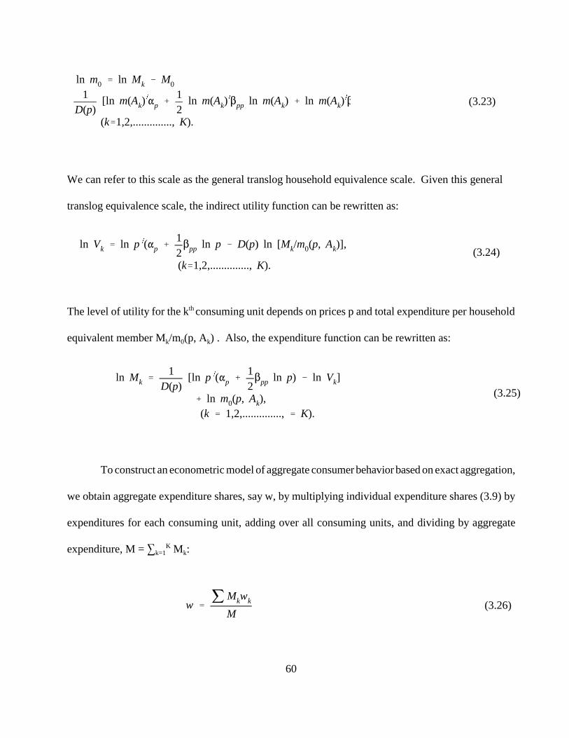
60

ln m0 � ln Mk � M0

1D(p)

[ln m(Ak)��p �

12

ln m(Ak)��pp ln m(Ak) � ln m(Ak)

��

(k�1,2,..............,K).

(3.23)

ln Vk � ln p �(�p �

12�pp ln p � D(p) ln [Mk/m0(p, Ak)],

(k�1,2,..............,K).(3.24)

ln Mk �

1D(p)

[ln p �(�p �

12�pp ln p) � ln Vk]

� ln m0(p, Ak),(k � 1,2,..............,� K).

(3.25)

w �

� Mkwk

M(3.26)

We can refer to this scale as the general translog household equivalence scale. Given this general

translog equivalence scale, the indirect utility function can be rewritten as:

The level of utility for the kth consuming unit depends on prices p and total expenditure per household

equivalent member Mk/m0(p, Ak) . Also, the expenditure function can be rewritten as:

To construct an econometric model of aggregate consumer behavior based on exact aggregation,

we obtain aggregate expenditure shares, say w, by multiplying individual expenditure shares (3.9) by

expenditures for each consuming unit, adding over all consuming units, and dividing by aggregate

expenditure, M = �k=1K Mk:

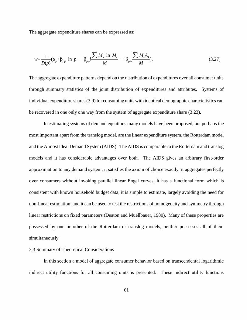
61

w� 1D(p)

(�p��pp ln p � �ppi� Mk ln Mk

M� �pA

� MkAk

M), (3.27)

The aggregate expenditure shares can be expressed as:

The aggregate expenditure patterns depend on the distribution of expenditures over all consumer units

through summary statistics of the joint distribution of expenditures and attributes. Systems of

individual expenditure shares (3.9) for consuming units with identical demographic characteristics can

be recovered in one only one way from the system of aggregate expenditure share (3.23).

In estimating systems of demand equations many models have been proposed, but perhaps the

most important apart from the translog model, are the linear expenditure system, the Rotterdam model

and the Almost Ideal Demand System (AIDS). The AIDS is comparable to the Rotterdam and translog

models and it has considerable advantages over both. The AIDS gives an arbitrary first-order

approximation to any demand system; it satisfies the axiom of choice exactly; it aggregates perfectly

over consumers without invoking parallel linear Engel curves; it has a functional form which is

consistent with known household budget data; it is simple to estimate, largely avoiding the need for

non-linear estimation; and it can be used to test the restrictions of homogeneity and symmetry through

linear restrictions on fixed parameters (Deaton and Muellbauer, 1980). Many of these properties are

possessed by one or other of the Rotterdam or translog models, neither possesses all of them

simultaneously

3.3 Summary of Theoretical Considerations

In this section a model of aggregate consumer behavior based on transcendental logarithmic

indirect utility functions for all consuming units is presented. These indirect utility functions

62

incorporate restrictions on individual behavior that result from maximization of utility functions subject

to budget constraints. Each individual consuming unit has an indirect utility function that is

homogeneous of degree zero in prices and expenditures, non-increasing in prices and non-decreasing

in expenditures. To include differences in individual preferences in the model of aggregate consumer

behavior, we allow the indirect utility functions for all consuming units to depend on attributes, such

as demographic characteristics, that vary among individual households.

Given a translog indirect utility function for each consuming unit, we derive the expenditure

shares for that unit by using Roy’s identity. This results in expenditure shares that can be expressed as

ratios of two functions that are linear in the logarithms of ratios of prices for all commodities to total

expenditure and attributes. The denominators of these ratios are functions that are the same for all

commodity groups. Under exact aggregation the individual expenditure shares are linear in functions

of attributes and total expenditures, so that the denominators are independent of total expenditures and

attributes and are the same for all individuals.

Under the exact aggregation condition, the translog indirect utility function is additive in

functions of the attributes and the total expenditures of the individual consuming unit and provides a

cardinal measure of individual welfare as well as an ordinal measure. Based on the indirect utility

function for each unit, we can explicitly solve for the expenditure function, giving the minimum

expenditures required to achieve the stipulated level of the individual welfare for given prices.

The expenditure function and indirect utility function can be employed in examining the impacts

of alternative economic policies on the welfare of the individual consuming unit. In fact, the concept

of equivalent and compensating variations in expenditures can be empirically tested. The equivalent

variation gives the additional or reduction in expenditures required to achieve the level of utility after

63

the change in policy. The compensating variation gives the additional or reduction in expenditures to

achieve required to achieve the level of utility before the change in policy, i.e., that which would exist

if the change actually taken place.

To derive aggregate expenditure shares, we multiply the individual expenditure shares by total

expenditures for each consuming unit, sum over all consuming units, and divide by aggregate

expenditure. The aggregate expenditure shares, can be expressed as ratios of two functions. The

denominators are the same as for individual expenditure shares. The numerators are linear in the

logarithms of prices, in a statistic of the distribution of expenditures over all consuming units � Mk ln

Mk/� Mk, and in the shares of all demographic groups in aggregate expenditures.

The individual expenditure shares are homogeneous of degree zero in prices and expenditures.

Given the restrictions implied by exact aggregation, this implies an additional N - 1 restrictions on the

parameters of the trans indirect utility functions, where N is the number of commodities. Second, the

sum of individual expenditure shares over all commodity groups is equal to unity. Given the exact

aggregation restrictions, there are N additional restrictions implied by summability. Third, the matrix

of compensated own -- and cross - - price effects must be symmetric. The implication of this is that

there are ½ (N - 1) restrictions on the parameters of the translog indirect utility functions.

Monotonicity of the indirect utility functions implies that the individual expenditure shares must

be non-negative. The indirect utility function is quasi convex, which implies that the individual

expenditure shares must be monotonic, or equivalently, that the matrix of compensated own -- and

cross - price substitution effects must be non-positive definite. It is always possible to choose prices

so that monotonicity of the indirect utility functions or non-negativity of the individual expenditure

shares is violated. Accordingly, we consider restrictions that imply monotonicity of the expenditure

64

G �

XX�Y

(3.28)

shares wherever they are non-negative.

3.4 Inequality in the Distribution of Household Consumption Expenditure

Economic well-being can be defined in terms of the capability individuals or households have

for potential consumption. Official income statistics are produced to reflect the consumption ability

of individuals and families, with money income used to proxy this consumption potential most

frequently. Garner (1993) pointed out that consumption may be a better measure of the actual

economic welfare of a household than its current income. The value of consumption sometimes can

be greater than annually reported income to the extent that households have accumulated savings or

accounting losses from a business (Sawhill, 1988; Garner, 1993), or that they are able to borrow against

future income. Thus, it may be safe to assume that consumption reflects material well-being in terms

of past, current, and expected future income, not just current income. How a household budgets its

income across different consumption groups can reflect the overall economic well-being of households

differently. Measuring the impact of marginal changes in different expenditures on the inequality of

total expenditures can provide important information, particularly for policy makers.

The inequality in the distribution of household consumption can be measured using the Gini

Coefficient. One of the most commonly calculated inequality statistics is the Gini Coefficient, which

is illustrated in figure 3.1. It is equal to the ratio of the area enclosed by the Lorenz curve and the

diagonal line of perfect equality to the total area below the diagonal.

Although the standard Gini lacks the flexibility to yield estimates that vary with individual’ aversion

65

A � �b

a

F(y)[1 � F(y)]dy (3.29)

A � 2�b

a

y[F(y) �

12

]f(y)dy (3.30)

to inequality (Atkinson, 1970), several authors including Kakwani (1980), Yitzhaki (1983), and

Donaldson and Weymark (1983) have developed versions of the extended Gini, a family of Ginis that

depend on social welfare functions in a manner resembling the Atkinson index. More recently, Lerman

and Yitzhaki (1984) derived a method for decomposing the Gini by income source and for calculating

the marginal effects on inequality from alternative sources.

In spite of the advantages of the Gini index and the existence of many derivations of the Gini,

calculating the Gini has remained a cumbersome process (Lerman and Yitzhaki, 1984). On this same

subject Deaton (1982) noted that it is considerably easier to calculate the Theil information index than

the Gini index. Lerman and Yitzhaki (1984) pointed out that this inconvenience in calculation along

with the ease in working with such variance measures as the coefficient of variation and the log of the

variance, have probably contributed to the frequent substitution of other measures for the Gini.

One formula for the absolute Gini as derived by Lerman and Yitzhaki (1983), is

where A is half of Gini’s expected mean difference, a is the lowest and b is the highest value of the

variable y, and F(y) is the commutative distribution of y. Using integration by part, with u = F(y)[1-

F(y)] and v = y, we obtain

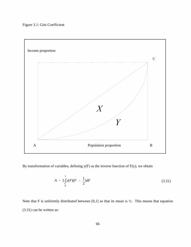
66

Income proportion

C

A Population proportion B

A � 2�1

0

y(F)(F �

12

)dF (3.31)

Figure 3.1: Gini Coefficient

By transformation of variables, defining y(F) as the inverse function of F(y), we obtain

Note that F is uniformly distributed between [0,1] so that its mean is ½. This means that equation

(3.31) can be written as:

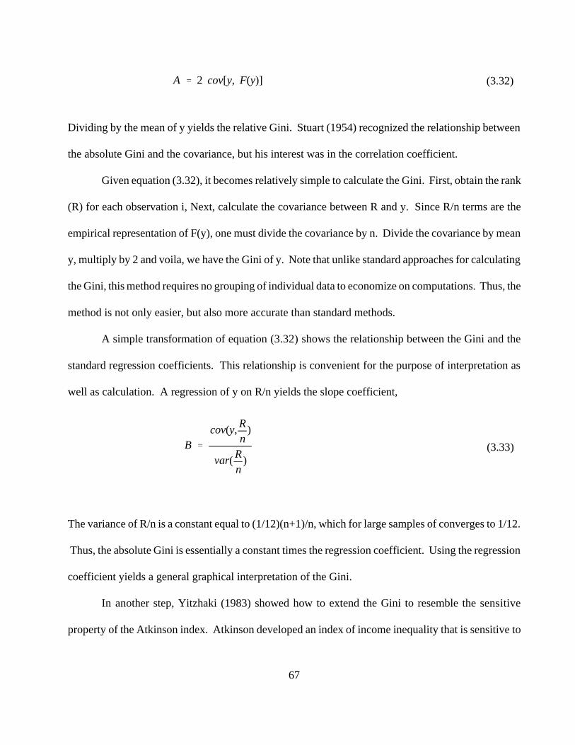
67

A � 2 cov[y, F(y)] (3.32)

B �

cov(y,Rn

)

var(Rn

)(3.33)

Dividing by the mean of y yields the relative Gini. Stuart (1954) recognized the relationship between

the absolute Gini and the covariance, but his interest was in the correlation coefficient.

Given equation (3.32), it becomes relatively simple to calculate the Gini. First, obtain the rank

(R) for each observation i, Next, calculate the covariance between R and y. Since R/n terms are the

empirical representation of F(y), one must divide the covariance by n. Divide the covariance by mean

y, multiply by 2 and voila, we have the Gini of y. Note that unlike standard approaches for calculating

the Gini, this method requires no grouping of individual data to economize on computations. Thus, the

method is not only easier, but also more accurate than standard methods.

A simple transformation of equation (3.32) shows the relationship between the Gini and the

standard regression coefficients. This relationship is convenient for the purpose of interpretation as

well as calculation. A regression of y on R/n yields the slope coefficient,

The variance of R/n is a constant equal to (1/12)(n+1)/n, which for large samples of converges to 1/12.

Thus, the absolute Gini is essentially a constant times the regression coefficient. Using the regression

coefficient yields a general graphical interpretation of the Gini.

In another step, Yitzhaki (1983) showed how to extend the Gini to resemble the sensitive

property of the Atkinson index. Atkinson developed an index of income inequality that is sensitive to

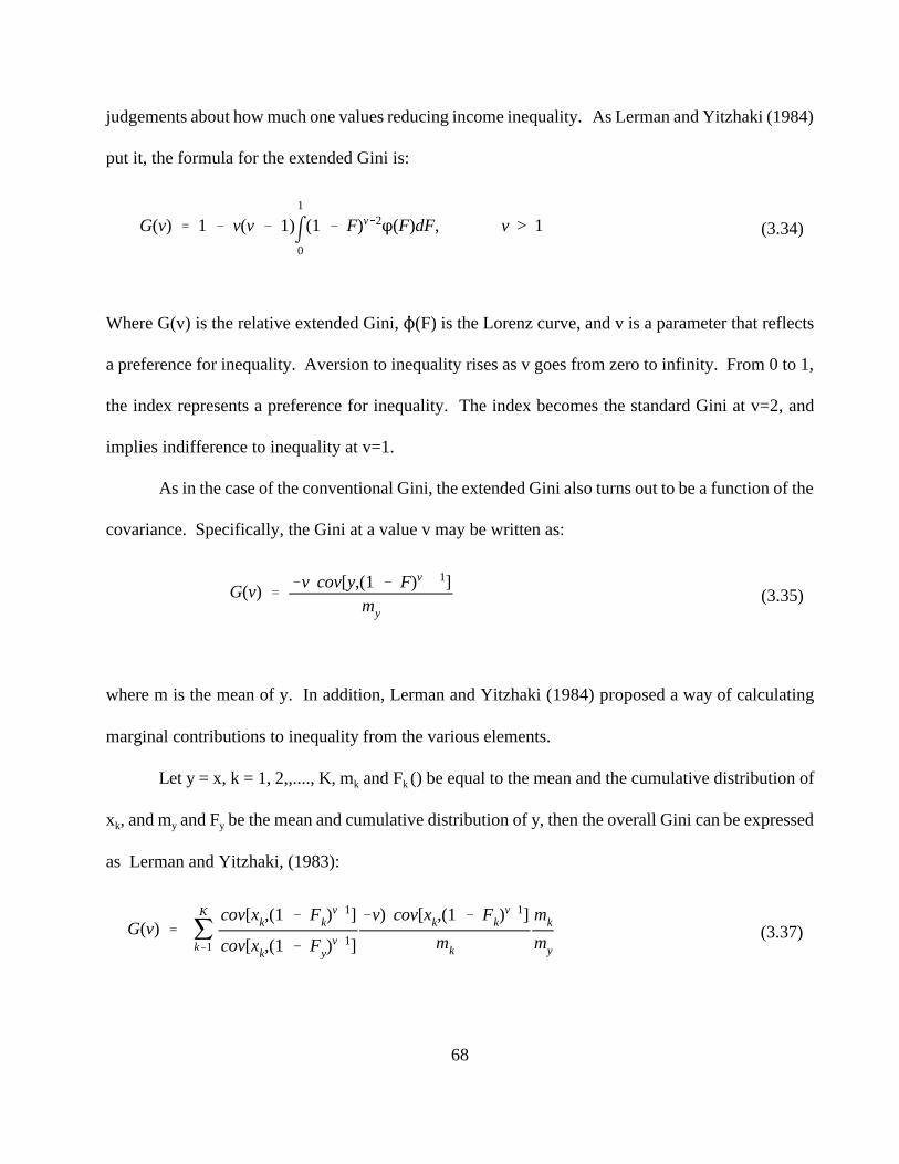
68

G(v) � 1 � v(v � 1)�1

0

(1 � F)v�2�(F)dF, v > 1 (3.34)

G(v) �

�v cov[y,(1 � F)v � 1]my

(3.35)

G(v) � �K

k�1

cov[xk,(1 � Fk)v�1]

cov[xk,(1 � Fy)v�1]

�v) cov[xk,(1 � Fk)v�1]

mk

mk

my

(3.37)

judgements about how much one values reducing income inequality. As Lerman and Yitzhaki (1984)

put it, the formula for the extended Gini is:

Where G(v) is the relative extended Gini, �(F) is the Lorenz curve, and v is a parameter that reflects

a preference for inequality. Aversion to inequality rises as v goes from zero to infinity. From 0 to 1,

the index represents a preference for inequality. The index becomes the standard Gini at v=2, and

implies indifference to inequality at v=1.

As in the case of the conventional Gini, the extended Gini also turns out to be a function of the

covariance. Specifically, the Gini at a value v may be written as:

where m is the mean of y. In addition, Lerman and Yitzhaki (1984) proposed a way of calculating

marginal contributions to inequality from the various elements.

Let y = x, k = 1, 2,,...., K, mk and Fk () be equal to the mean and the cumulative distribution of

xk, and my and Fy be the mean and cumulative distribution of y, then the overall Gini can be expressed

as Lerman and Yitzhaki, (1983):

69

� �K

k�1CkGkSk (3.36)

Where Ck is the Gini correlation between element k and the rank of total y, Gk is the Gini element k,

and Sk is the mean of x divided by the mean of y (or x’s share of y). The Gini correlation has properties

that are similar to Pearson’s and the rank correlation. Lerman and Yitzhaki (1983) pointed out that

Pearson correlation and Gini correlation between component x and the rank of y have the same

numerators, but the Pearson numerator correlation deflates the cov(xk, Rk) by a constant (equal to the

standard deviation of the rank of xk ) while the Gini correlation uses the Gini of xk as denominator. The

result yields a convenient interpretation in the case of the standard Gini (v = 2), where Gk may be

represented by the ratio of the slope coefficient from the regression of xk and Ry the slope coefficient

from the regression of xk and Rk, according to Lerman and Yitzhaki.

The key rationale for studying decomposition by source is to learn how changes in particular

income sources will affect overall income inequality. The theoretical framework explained in this

section extends derivations reported by Kakwani (1977) and Shorrocks (1982) in which a given

source’s contribution is the product of the share of total income and a term called the pseudo-Gini. The

pseudo-Gini appears as the product of the source itself and the correlation between the source and the

rank of total income (Lerman and Yitzhaki, 1984) . It also has been shown that a similar result holds

for the extended Gini, a measure that is like the Atkinson (1970) index in permitting alternative weights

in different parts of income distributions (Lerman and Yitzhaki, 1984) .

70

CHAPTER 4: DATA AND DATA ORGANIZATION

4.1 Introduction

This chapter discusses the source, organization and transformation of data. It is divided into

three additional sections. The source of the data and the method in which the data are collected are

presented in section 4.2. Section 4.3 discusses how the data are downloaded from one form of storage

to another form of storage using the Job Control (JCL) and Statistical Analysis System Languages

(SAS), including the creation of the SAS data set. The transformation of the cross sectional data

downloaded from the external medium of storage to panel data is presented in section 4.4.

4.2 Source of Data

The key ingredient to the evaluation of consumption-based inequality is a disaggregated data

set on consumer expenditures. In the United States, the only source of such data is the consumer

expenditure surveys. The Census Bureau conducts this survey on behalf of the Bureau of Labor

Statistics. The consumer expenditure data are collected from a national probability sample of

households designed to represent the total civilian noninstitutional population and a portion of

institutional population living in selected types of group quarters. Housing units occupied by students

are also surveyed. The interview sample, selected on a rotating panel basis, is targeted at 5000

consumer units per quarter. Each quarter one-fifth of the sample is new to the survey. After being

interviewed for five consecutive quarters, a panel is dropped from the survey. The fifth quarter overlaps

with the first quarter of the next year.

The rotating sample design of the interview survey has an effect on the structure of the data files

and the use of the data itself . This is described by the Bureau as a distinction between calendar period

and collection period. Respondents are asked to report expenditures made since the first of the month

71

three months prior to the interview month. For example, if the Consumer Unit is interviewed in January

of 1991, they are reporting expenditures for October, November, and December of 1990. The period

between October 1 and December 31 is referred as the reference period for the interview. Files on the

public use tapes are organized and identified by collection period, and the actual period of expenditure

is not reflected.

The data upon which this study is based are drawn from the 1980 through 1994 Interview

Surveys which include consumer characteristics and expenditures. The consumer characteristics or

family characteristics data pertain to age, sex, race, martial status, education, and consumer unit

relationship for each member. The expenditure file, which is referred as ‘Detailed Expenditure’,

provides expenditure data at the most detailed level available. The mechanics of downloading the

above two files and the creation of the SAS data set are presented in the next section.

4.3 Data Organization and Manipulation

Two files, consumer characteristics and expenditure files, were downloaded from a reel tape

obtained from the BLS, to cartridge tapes by quarter using job control computer language (JCL). A

permanent SAS data set was created by merging the two files, the consumer characteristics and

expenditures by the unique consumer identification number assigned to each household . Appendix P-1

illustrates the JCL and SAS programs used to download and merge files, including that for creating a

permanent SAS data set.

As stated in section 4.2, one problem with the structure is that the reference and collection

periods of the data are different. The collection period is not consistent with the true price of the

commodity for which the expenditure is made. The questions are written in such a way to ask the

respondent how much she/he spent on a particular commodity in the last three months. Since this study

72

uses prices and price data are collected by month, it is important to make the date in which the

expenditure was made consistent with price on the actual date of purchase. To do that we divided each

quarter by three and back dated to the month of purchase. Once the data is disaggregated by month,

the next task is to merge the data set with the data set for prices. Data for the prices of the commodities

used in this study are obtained from BLS database using the internet access. All prices are reported as

indexes. Appendix P-1 through appendix P9 show the SAS programs used to accomplish the above

computing

4.4 The Transformation of Time-Series-Cross Section Data to Panel Data

The transformation of cross section data to panel data is based on the theoretical framework

described in chapter 3. The Consumer Expenditure Survey is not a panel; the same individual

households are not followed through long period of time. Participation of a household is limited to only

five quarters after adjustments. However, the survey is a continuous operation so that it provides a

random sample of the population each quarter (subject to the exclusion and inclusion of certain

households every quarter). Our data represents the period between 1980 and 1994. Hence, although

we cannot track individual households, we can track groups of households. In particular, if we take age

as age of the household head, we can look at the average behavior of, say, those 25 years old in 1980,

26 years old in 1981, etc. Given the linear in parameter functional forms, mean cohort behavior

reproduces the form of individual behavior and the cohorts can thus effectively be treated as

individuals. If the price of lifetime utility is constant for all members of the cohort from one year to the

next, then its mean is constant for the cohort as a whole. Hence, the sample mean from the survey will

be a consistent estimator of the same quantity from year to year, with a precision determined by the

sample design (Deaton, 1985). Based on the conclusion made by Deaton (1985), the cohorts means can

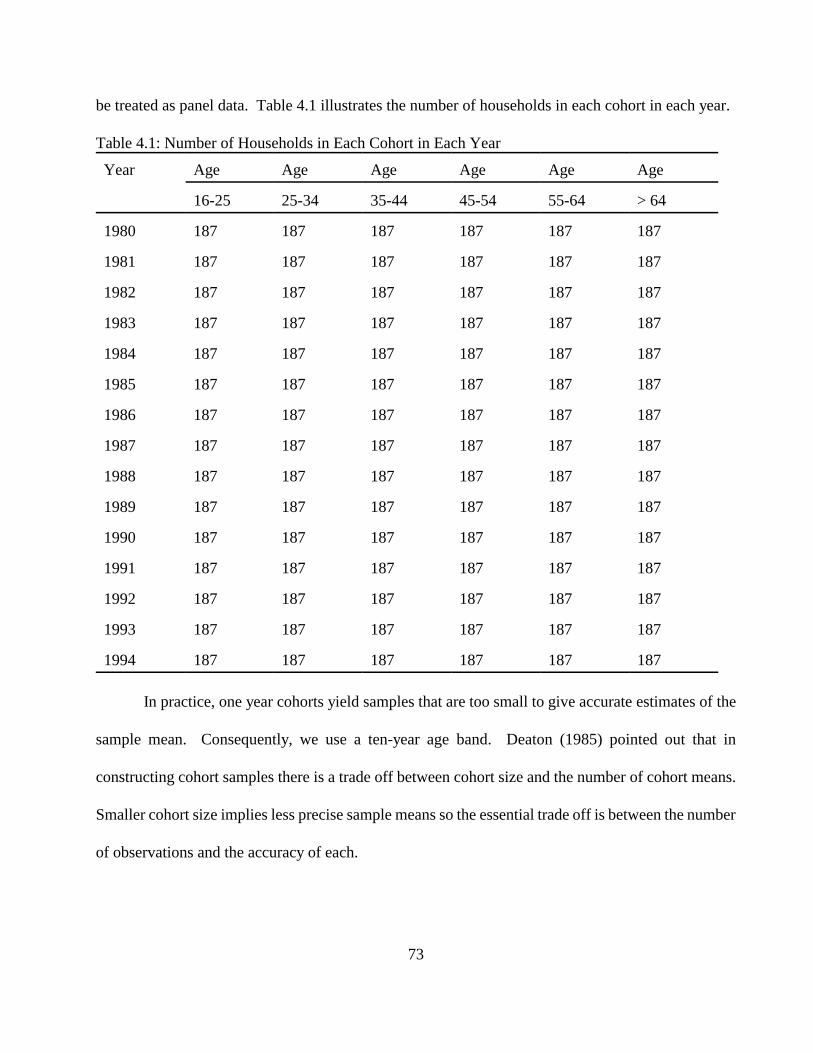
73

be treated as panel data. Table 4.1 illustrates the number of households in each cohort in each year.

Table 4.1: Number of Households in Each Cohort in Each Year

Year Age Age Age Age Age Age

16-25 25-34 35-44 45-54 55-64 > 64

1980 187 187 187 187 187 187

1981 187 187 187 187 187 187

1982 187 187 187 187 187 187

1983 187 187 187 187 187 187

1984 187 187 187 187 187 187

1985 187 187 187 187 187 187

1986 187 187 187 187 187 187

1987 187 187 187 187 187 187

1988 187 187 187 187 187 187

1989 187 187 187 187 187 187

1990 187 187 187 187 187 187

1991 187 187 187 187 187 187

1992 187 187 187 187 187 187

1993 187 187 187 187 187 187

1994 187 187 187 187 187 187

In practice, one year cohorts yield samples that are too small to give accurate estimates of the

sample mean. Consequently, we use a ten-year age band. Deaton (1985) pointed out that in

constructing cohort samples there is a trade off between cohort size and the number of cohort means.

Smaller cohort size implies less precise sample means so the essential trade off is between the number

of observations and the accuracy of each.

74

Yit � � � �Xit � �it (5.1)

CHAPTER 5: Econometric Model and Estimation Results

5.1 Introduction

This chapter has three sections. Section 5.2 presents the econometric model and its

implementation to estimate the impact of demographic characteristics on individual household

expenditure patterns. The results of the empirical estimations are illustrated and discussed in section

5.3. Section 5.4 presents the summary and conclusions.

5.2 Econometric Model

The general econometric model to measure the impact of prices and demographic characteristics

on the expenditure pattern of household units is specified as:

Where Y is the a vector of expenditure shares used as dependent variables. The expenditures are

divided among eight commodity groups. X represents a vector of independent variables, a nonrandom

function of prices, expenditure and demographic characteristics. � is an unobserved random disturbance

that is functionally independent of the explanatory variables. The disturbance may result from errors

in implementation, random elements in the determination of consumer preferences not reflected in the

list of attributes of consuming units, errors in measurements of individual expenditure shares,

specification error, or errors in the design and collection of data. We assume that the individual

disturbances have an expected value equal to zero. Since the individual expenditure shares for all

commodities sum to unity for each consuming unit in each time period, the unobservable random

disturbances for all commodities sum to zero. These disturbances are distributed normally with mean

zero and covariance matrix �. We also assume that the covariance matrix of the individual

75

disturbances has the rank equal to N - 1, where N is the number of commodities. Finally, we assume

that disturbances corresponding to distinct observations are uncorrelated. The above model is specified

for eight commodity groups in which eight equations are specified and only seven equations are

required for a complete model. Since the equations for the budget shares are generated from the

indirect translog utility function, the parameters satisfy equality and symmetry restrictions that are

strictly analogous to the corresponding restrictions the direct translog utility function..

5.2.1 Dependent Variable Descriptions

There are seven dependent variables one for each equation. As stated in chapter three, these

expenditure shares are derived by the logarithmic form of Roy’s identity. Table 5.1 gives descriptions

of the dependent variables which are the budget shares.

Table 5.1: Dependent Variables

VARIABLE DESCRIPTION

FOOD_SHARE SHARE OF EXPENDITURE ON FOOD AND BEVERAGES.

HOUSING_SHARE AGGREGATED EXPENDITURE SHARE ON HOUSING.

APPAREL_SHARE EXPENDITURE SHARE ON APPAREL.

ENTER_SHARE EXPENDITURE SHARE ON ALL FORMS OF ENTERTAINMENT.

HEALTH_SHARE EXPENDITURE SHARE ON HEALTH.

TRANS_SHARE EXPENDITURE SHARE ON TRANSPORTATION.

UTILITY_SHARE EXPENDITURE SHARE ON UTILITY

5.2.2 Independent Variables

There are twenty five independent variables of which 17 are dummy variables. We have four

categories of demographic characteristics: age of head of the household, family size, geographic region

of residence, and race. The logarithms of price indexes for each commodity group along with the

logarithms of total expenditure for each commodity group are also defined as explanatory variables.

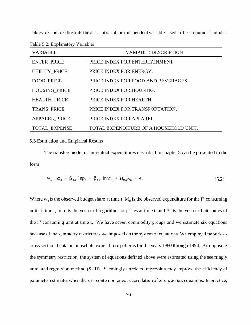
76

wit ��P � �PP lnpit � �PP lnMit � BPAAit � �it (5.2)

Tables 5.2 and 5.3 illustrate the description of the independent variables used in the econometric model.

Table 5.2: Explanatory Variables

VARIABLE VARIABLE DESCRIPTION

ENTER_PRICE PRICE INDEX FOR ENTERTAINMENT

UTILITY_PRICE PRICE INDEX FOR ENERGY.

FOOD_PRICE PRICE INDEX FOR FOOD AND BEVERAGES.

HOUSING_PRICE PRICE INDEX FOR HOUSING.

HEALTH_PRICE PRICE INDEX FOR HEALTH.

TRANS_PRICE PRICE INDEX FOR TRANSPORTATION.

APPAREL_PRICE PRICE INDEX FOR APPAREL

TOTAL_EXPENSE TOTAL EXPENDITURE OF A HOUSEHOLD UNIT.

5.3 Estimation and Empirical Results

The translog model of individual expenditures described in chapter 3 can be presented in the

form:

Where wit is the observed budget share at time t, Mit is the observed expenditure for the ith consuming

unit at time t, ln pit is the vector of logarithms of prices at time t, and Ait is the vector of attributes of

the ith consuming unit at time t. We have seven commodity groups and we estimate six equations

because of the symmetry restrictions we imposed on the system of equations. We employ time series -

cross sectional data on household expenditure patterns for the years 1980 through 1994. By imposing

the symmetry restriction, the system of equations defined above were estimated using the seemingly

unrelated regression method (SUR). Seemingly unrelated regression may improve the efficiency of

parameter estimates when there is contemporaneous correlation of errors across equations. In practice,

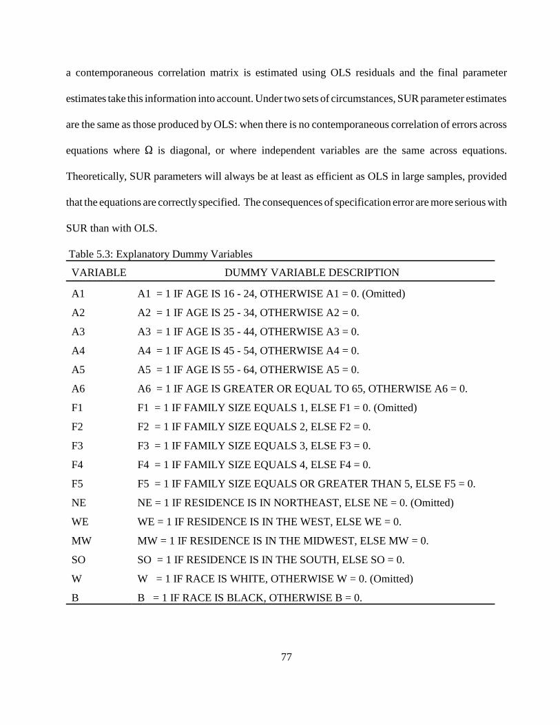
77

a contemporaneous correlation matrix is estimated using OLS residuals and the final parameter

estimates take this information into account. Under two sets of circumstances, SUR parameter estimates

are the same as those produced by OLS: when there is no contemporaneous correlation of errors across

equations where is diagonal, or where independent variables are the same across equations.

Theoretically, SUR parameters will always be at least as efficient as OLS in large samples, provided

that the equations are correctly specified. The consequences of specification error are more serious with

SUR than with OLS.

Table 5.3: Explanatory Dummy Variables

VARIABLE DUMMY VARIABLE DESCRIPTION

A1 A1 = 1 IF AGE IS 16 - 24, OTHERWISE A1 = 0. (Omitted)

A2 A2 = 1 IF AGE IS 25 - 34, OTHERWISE A2 = 0.

A3 A3 = 1 IF AGE IS 35 - 44, OTHERWISE A3 = 0.

A4 A4 = 1 IF AGE IS 45 - 54, OTHERWISE A4 = 0.

A5 A5 = 1 IF AGE IS 55 - 64, OTHERWISE A5 = 0.

A6 A6 = 1 IF AGE IS GREATER OR EQUAL TO 65, OTHERWISE A6 = 0.

F1 F1 = 1 IF FAMILY SIZE EQUALS 1, ELSE F1 = 0. (Omitted)

F2 F2 = 1 IF FAMILY SIZE EQUALS 2, ELSE F2 = 0.

F3 F3 = 1 IF FAMILY SIZE EQUALS 3, ELSE F3 = 0.

F4 F4 = 1 IF FAMILY SIZE EQUALS 4, ELSE F4 = 0.

F5 F5 = 1 IF FAMILY SIZE EQUALS OR GREATER THAN 5, ELSE F5 = 0.

NE NE = 1 IF RESIDENCE IS IN NORTHEAST, ELSE NE = 0. (Omitted)

WE WE = 1 IF RESIDENCE IS IN THE WEST, ELSE WE = 0.

MW MW = 1 IF RESIDENCE IS IN THE MIDWEST, ELSE MW = 0.

SO SO = 1 IF RESIDENCE IS IN THE SOUTH, ELSE SO = 0.

W W = 1 IF RACE IS WHITE, OTHERWISE W = 0. (Omitted)

B B = 1 IF RACE IS BLACK, OTHERWISE B = 0.

78

Economic theory requires that the individual expenditure shares be homogeneous of degree zero

in prices and total expenditures, the sum of the individual expenditure shares over all commodity

groups, be equal to unity, the matrix of compensated own and cross-price substitution effects be

symmetric, and the individual expenditure shares be non-negative. The translog model with the above

conditions imposed is estimated using the Zellner Regression Method and the results are illustrated in

tables 5.5 - 5.11. To avoid the problem of perfect multicollinearity, one dummy variable from each

category is omitted. The significant variables are shaded in the tables and the degree of significance

is indicated by asterisks in the last column of each table.

5.3.1 Food and Beverages

Prices play an important role in the allocation of budget share for the consumption of food and

beverages. The coefficient for FOOD_PRICE, price for food and beverages indicates that as price

increases by one unit, the level of expenditure share for food and beverages increases by 0.075 (see

table 5.4) indicating inelastic demand. Other prices such as the prices of health care and housing have

negative effect indicating substitutability in the distribution of share of expenditures. The coefficient

for apparel is 99% significant with a positive sign. Households tend to allocate less for food as the

amount of their total expenditure rises. The coefficient for the prices of entertainment, utility, and

transportation are not statistically significant.

As indicated by the coefficient for A2, the food expenditure share for the head of the household

age 25-35 is less by 0.005597 compared with the expenditure share for a household headed by an

individual aged 16-24 (Table 5.4). This difference may be attributed to the difference in life styles

between these two age groups. The individual aged 16-24 may be spending more money on food and

beverages away from home in outlets such as restaurants and hotels which are more expensive or it

79

could be that the income for age group 16-24 is smaller and, typically, people with smaller incomes

spend a greater proportion of that income on food. Households headed by individuals aged 35-44, 45-

54, and 55-64 have relatively larger shares of expenditures on food and beverages than the 16-24 age

group. Estimates representing family size show that families with 2, 3, 4, and 5 family members have

larger expenditure shares for food and beverages than households with a single person. The more the

members the more the expenditure share on food and beverages. In terms of residence, households

living in the west, south and mid-west allocate relatively less to food than do households residing in

the northeast geographical region. This may be related to differences in prices, income, life style or

culture.

The dummy variable representing race shows that the expenditure share decreases when the

head of the household is black instead of white. Actually, the result should have been the other way

around because of that blacks earn less than whites and lower income people tend to spend more of their

incomes on food. One possible explanation for this phenomenon is that since many low income

families receive subsidies in the form of food stamps they do not need to allocate more cash for food

and this study does not include expenditures in other forms other than cash. However, lower income

people may allocate more of their income on food items such as potatoes, chicken, and others which

are priced low. Since higher income people are more educated and health conscious their share of

expenditure could be higher because the type of food they consume may be more expensive. These data

include food at home, food away from home, beverages, and other expenditures related to food, so that

consumption patterns could also affect the results.

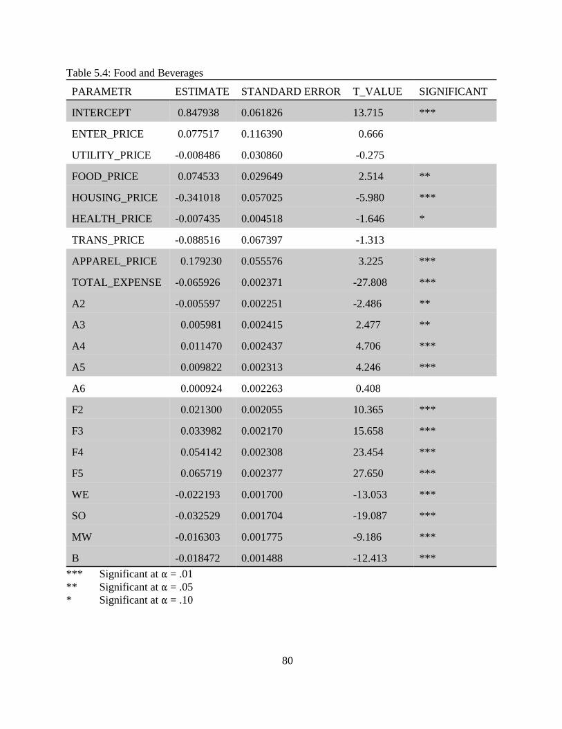
80

Table 5.4: Food and Beverages

PARAMETR ESTIMATE STANDARD ERROR T_VALUE SIGNIFICANT

INTERCEPT 0.847938 0.061826 13.715 ***

ENTER_PRICE 0.077517 0.116390 0.666

UTILITY_PRICE -0.008486 0.030860 -0.275

FOOD_PRICE 0.074533 0.029649 2.514 **

HOUSING_PRICE -0.341018 0.057025 -5.980 ***

HEALTH_PRICE -0.007435 0.004518 -1.646 *

TRANS_PRICE -0.088516 0.067397 -1.313

APPAREL_PRICE 0.179230 0.055576 3.225 ***

TOTAL_EXPENSE -0.065926 0.002371 -27.808 ***

A2 -0.005597 0.002251 -2.486 **

A3 0.005981 0.002415 2.477 **

A4 0.011470 0.002437 4.706 ***

A5 0.009822 0.002313 4.246 ***

A6 0.000924 0.002263 0.408

F2 0.021300 0.002055 10.365 ***

F3 0.033982 0.002170 15.658 ***

F4 0.054142 0.002308 23.454 ***

F5 0.065719 0.002377 27.650 ***

WE -0.022193 0.001700 -13.053 ***

SO -0.032529 0.001704 -19.087 ***

MW -0.016303 0.001775 -9.186 ***

B -0.018472 0.001488 -12.413 ***

*** Significant at � = .01** Significant at � = .05* Significant at � = .10

81

5.3.2 Housing and Housing Service

The price variable for housing, HOUSING_PRICE has a positive relation with the expenditure

share for housing. As the price increases by one unit the expenditure share increases by 0.050 (Table

5.5). Expenditure on housing is a long term planned commitment and one cannot react to changes in

prices right away. If the prices of maintenance goes up, the owner has little choice, except to pay for

it in order to protect his or her investment and/or life style. On the other hand, the effect of data

aggregation might have resulted in positive estimate than a negative one, since expenditure share for

housing includes the mortgage/rent, expenditure on furniture and related items, housing maintenance,

and domestic serves. While prices for utilities, health care, and total expenditures have negative

coefficient estimates, prices for transportation and apparel have positive coefficients. The coefficients

of the other price variables are not statistically significant.

Dummy variables representing the age category indicate that expenditure share for housing and

housing related services is relatively higher for households headed by individuals aged 25-34 and 35-44

when compared with the head os a household age 16-24. In most cases people between 25-55 maintain

a larger family and make investments in housing and real estate. So, increases in the age of the head

of the household, at least until 50, may be one possible factor for the increase in expenditure share for

housing and housing related services such as rent, mortgage, maintenance, and other services. Also,

the two age groups mentioned were buying homes in an era when costs increasing. The fact that 16-24

age group is a typical low income group, may be one more reason for having less expenditure share than

the next two age groups. Estimates for the variables representing ages 45-54, 55-64 and 65 or over are

not statistically significant.

Increases in the family size have negative effects on expenditure share for housing. From the

82

simple inspection of this expenditure data we observe that housing takes a high share of the household’s

budget. Households with more family members may be forced to allocate their resources for other basic

necessities rather than to bigger or more expensive homes and services. Also, the more people in the

family the greater the possibility that some of the services could be rendered by the family members,

which may help reduce the cost of housing.

Expenditure share for housing and housing related services is less in the West and South

geographic regions than the Northeast. This phenomenon could be attributed to the difference in the

climatic conditions of the regions, especially during winter. Also, the differences in prices of housing

and the wages rate may be a factor, as well as differences in land values. Households living in the mid-

west geographical region have a higher expenditure share than those living in the northeast region.

The relative expenditure share on housing and housing related services by a household headed

by a black person is less than the household headed by a white individual. This can be directly attributed

to the low proportion of income distribution for blacks. According to Charles Nelson (1994) in 1967

the Black-White household income ratio was 0.58. In 1990, 23 years later, this ratio was only slightly

higher (0.62). This fact directly supports the our findings regarding expenditure inequality between

blacks and whites on housing and housing related investments with its root cause being inequality in

earnings. Since blacks earn less and spend a smaller share of that on housing, probably means that they

1. live in inferior housing, and 2. a greater proportion live in government subsidized housing.

5.3.3 Apparel

The own price for apparel is not statistically significant (Table 5.6). While estimates for the

prices of entertainment, and housing are positive, estimate for the price of health care is negative. As

83

Table 5.5: Housing and Housing Services

PARAMETR ESTIMATE STANDARD ERROR T_VALUE SIGNIFICANCE

INTERCEPT 0.294487 0.104539 2.817 ***

ENTER_PRICE -0.008486 0.030860 -0.275

UTILITY_PRICE -0.113629 0.031441 -3.614 ***

FOOD_PRICE -0.028550 0.018834 -1.516

HOUSING_PRICE 0.050135 0.023511 2.132 **

HEALTH_PRICE -0.015791 0.004999 -3.159 ***

TRANS_PRICE 0.145934 0.054527 2.676 ***

APPAREL_PRICE 0.048422 0.028591 1.694 *

TOTAL_EXPENSE -0.031175 0.004430 -7.037 ***

A2 0.044804 0.004111 10.900 ***

A3 0.040076 0.004408 9.092 ***

A4 0.004809 0.004418 1.089

A5 -0.006514 0.004214 -1.546

A6 -0.006008 0.004175 -1.439

F2 -0.009668 0.003829 -2.525 **

F3 -0.009329 0.004032 -2.314 **

F4 -0.010969 0.004291 -2.557 **

F5 -0.026052 0.004435 -5.875 ***

WE -0.023951 0.003256 -7.355 ***

SO -0.035285 0.003253 -10.484 ***

MW 0.016101 0.003381 4.762 ***

B -0.005210 0.002844 -1.832 *

*** Significant at � = .01** Significant at � = .05* Significant at � = .10

84

expenditure increases the share of budget for apparel decreases. The estimates for the other variables

are statistically insignificant.

Expenditure shares on apparel tend to decrease as the age of the head of the household increases

except for the 55-64 age group. Since apparel is an expendable and non-basic item, people may shift

their resource to something more important or to something which has a return. Also, the life styles of

people in different age groups are different. It appears households between age 55-64 spend more and

those age 65 or over spend relatively less than the household between age 16-24. Households with two

or three family members spend a smaller share of their income on apparel than household with a single

individual, which is contrary to expectations in that families with more members would seem to need

more clothing, but they also need more food, medical services, etc. Households living in the Western

geographical region allocate relatively more and those living in the south have relatively less expenditure

shares than those living in the Northeastern geographical region. This phenomenon may be attributed

to differences in life style of people living in different regions and also differences in climate of the

geographical regions. In the case of race, blacks tend to have relatively larger expenditure shares on

apparel than whites.

5.3.4 Entertainment

Table 5.7 illustrates the estimates for entertainment. Entertainment is a fast growing industry,

both in terms demand and supply. As the price of entertainment increases by a unit the expenditure share

for entertainment decreases by 0.341 and its significant level is over 99%. Coefficients for prices of food

and beverages, housing, and apparel indicate that they are complements for entertainment, i.e., they have

positive coefficients. When the entertainment activity takes place at home, more is allocated to pay for

domestic services or for furniture or electronic appliances. Differences in the age of the head of a

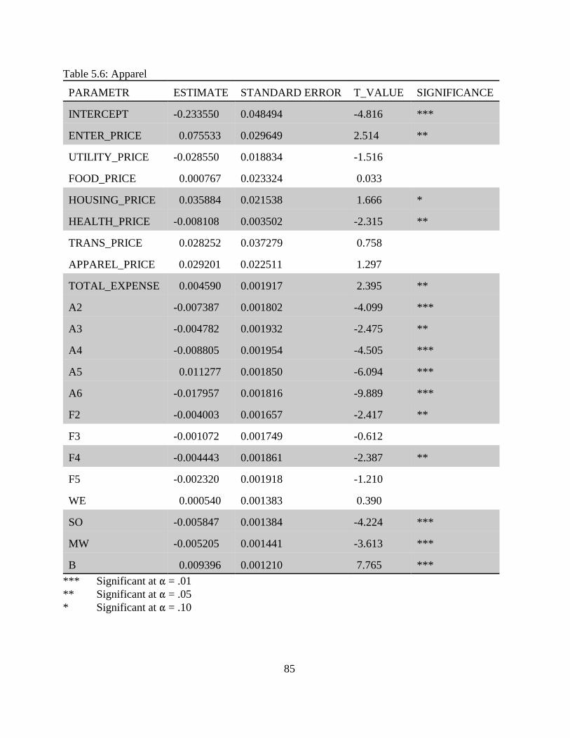
85

Table 5.6: Apparel

PARAMETR ESTIMATE STANDARD ERROR T_VALUE SIGNIFICANCE

INTERCEPT -0.233550 0.048494 -4.816 ***

ENTER_PRICE 0.075533 0.029649 2.514 **

UTILITY_PRICE -0.028550 0.018834 -1.516

FOOD_PRICE 0.000767 0.023324 0.033

HOUSING_PRICE 0.035884 0.021538 1.666 *

HEALTH_PRICE -0.008108 0.003502 -2.315 **

TRANS_PRICE 0.028252 0.037279 0.758

APPAREL_PRICE 0.029201 0.022511 1.297

TOTAL_EXPENSE 0.004590 0.001917 2.395 **

A2 -0.007387 0.001802 -4.099 ***

A3 -0.004782 0.001932 -2.475 **

A4 -0.008805 0.001954 -4.505 ***

A5 0.011277 0.001850 -6.094 ***

A6 -0.017957 0.001816 -9.889 ***

F2 -0.004003 0.001657 -2.417 **

F3 -0.001072 0.001749 -0.612

F4 -0.004443 0.001861 -2.387 **

F5 -0.002320 0.001918 -1.210

WE 0.000540 0.001383 0.390

SO -0.005847 0.001384 -4.224 ***

MW -0.005205 0.001441 -3.613 ***

B 0.009396 0.001210 7.765 ***

*** Significant at � = .01** Significant at � = .05* Significant at � = .10

86

household is a factor in the allocation of resources for entertainment purpose. People in the age groups

25-34 and 35-44 tend to have relatively more expenditure shares for entertainment than people between

the age 16-24. It is not uncommon for people between 25-45 to have a family and choose a form of

entertainment like traveling, out door entertainment and others which are more expensive. The

coefficients for households aged 45 to 64 are not significant, whereas the coefficient for those

households aged 65 or older is negative. Households residing in the west and mid-west tend to allocate

relatively more money for entertainment than those living in northeast and the south. The environments

which these households live under could be a factor in the difference. Again, blacks allocate relatively

less resources for entertainment than whites. On one hand, differences in income could be a factor but,

on the other hand, preference and tastes may determine the kind of entertainment blacks tend consume.

5.3.5 Heath Care and Health Related Services

We can easily observe from the data set used in this study that in the last fifteen years alone the

prices for health care and health care related services have doubled. Government expenditures on

medicare and medicaid, and health insurance rates also have increased. Table 5.8 shows that almost all

estimates except one for personal care and education have negative coefficients, which indicates that

their expenditure shares can be substituted for the expenditure share of health care. The coefficient for

price of health care is not significant, a surprising finding since rising health care costs have been blamed

for increasing expenditures. However, insurance, medicare, and medicaid pay for a large share of health

care.

The coefficients for age variables between 25-45 are not statistically significant, however ages

45 and over spend relatively more on health care as their age increases. Naturally, as a person gets older

the chance of having a health problem also increases. By almost any measure, the elderly comprise the

87

Table 5.7: Entertainment

PARAMETR ESTIMATE STANDARD ERROR T_VALUE SIGNIFICANCE

INTERCEPT -0.101563 0.049748 -2.042 **

ENTER_PRICE -0.341018 0.057025 -5.980 ***

UTILITY_PRICE 0.050135 0.023511 2.132 **

FOOD_PRICE 0.035884 0.021538 1.666 *

HOUSING_PRICE 0.301138 0.045866 6.566 ***

HEALTH_PRICE -0.006835 0.003609 -1.894 *

TRANS_PRICE -0.160623 0.051228 -3.135 ***

APPAREL_PRICE 0.123587 0.031179 3.964 ***

TOTAL_EXPENSE -0.000649 0.001881 -0.345

A2 0.003056 0.001792 1.705 *

A3 0.003654 0.001921 1.902 *

A4 0.001013 0.001942 0.522

A5 -0.001395 0.001841 -0.758

A6 -0.007458 0.001796 -4.152 ***

F2 -0.005380 0.001631 -3.297 ***

F3 -0.007160 0.001722 -4.158 ***

F4 -0.005998 0.001832 -3.273 ***

F5 -0.006589 0.001885 -3.496 ***

WE 0.000220 0.001344 0.164

SO -0.003246 0.001346 -2.408 **

MW 0.006426 0.0001405 4.574 ***

B -0.012547 0.001176 -10.669 ***

*** Significant at � = .01** Significant at � = .05* Significant at � = .10

88

age group most affected by problems of ill health. According to Viscusi (1979) only 20% of those aged

65 to 75 are free of chronic illness and less than 13% of those aged 75 and older are classified healthy.

In terms of limitations on their normal activities, far fewer elderly are affected. Less than one fourth of

those aged 75 and over are not physically able to carry out their daily activities. These assertions directly

and indirectly support the findings concerning the increase in share of expenditures on health as the

individual gets older. The results also show that as the number of people in the family increases the

amount of expenditure shares also increases. For family size two and three the estimated coefficients

are statistically significant, but not for larger family size. Health care expenditure shares for households

living in the western and mid-western geographical regions are relatively less than the ones living in the

northeastern geographical region. This difference can be attributed at least in part to the higher price

index for medical services in the northeastern geographical region. The race variable indicates that

blacks allocate less on health care services than whites. Households earning below certain amount of

income get free health benefits from the government and other public programs. A good proportion of

the black population may rely on these programs for their health care services.

5.3.6 Transportation

The need of transportation has become a basic necessity in the life styles of industrialized

societies. The information age might be able to reverse this phenomenon in the future. As indicated in

table 5.9, as the price of transportation goes up the expenditure shares for transportation also increase.

This is probably due to transportation being vital to the household’s livelihood, making the the response

inelastic. The prices of food and personal care and education are negatively related to the share of

expenditures on transportation, while the remainder of the price variables, and the total expenditures

are positively related.

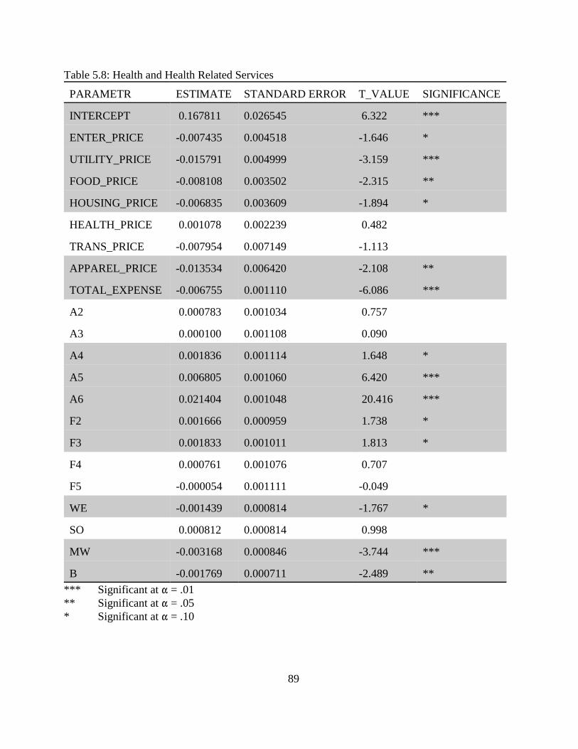
89

Table 5.8: Health and Health Related Services

PARAMETR ESTIMATE STANDARD ERROR T_VALUE SIGNIFICANCE

INTERCEPT 0.167811 0.026545 6.322 ***

ENTER_PRICE -0.007435 0.004518 -1.646 *

UTILITY_PRICE -0.015791 0.004999 -3.159 ***

FOOD_PRICE -0.008108 0.003502 -2.315 **

HOUSING_PRICE -0.006835 0.003609 -1.894 *

HEALTH_PRICE 0.001078 0.002239 0.482

TRANS_PRICE -0.007954 0.007149 -1.113

APPAREL_PRICE -0.013534 0.006420 -2.108 **

TOTAL_EXPENSE -0.006755 0.001110 -6.086 ***

A2 0.000783 0.001034 0.757

A3 0.000100 0.001108 0.090

A4 0.001836 0.001114 1.648 *

A5 0.006805 0.001060 6.420 ***

A6 0.021404 0.001048 20.416 ***

F2 0.001666 0.000959 1.738 *

F3 0.001833 0.001011 1.813 *

F4 0.000761 0.001076 0.707

F5 -0.000054 0.001111 -0.049

WE -0.001439 0.000814 -1.767 *

SO 0.000812 0.000814 0.998

MW -0.003168 0.000846 -3.744 ***

B -0.001769 0.000711 -2.489 **

*** Significant at � = .01** Significant at � = .05* Significant at � = .10

90

Expenditure shares on transportation decrease as both the age and the number of people in the

household increase. As both age and family size increase, people may find ways to reduce the

transportation costs such as trading vehicle less frequently and by doing more things at home.

Households residing in the west and south have a higher expenditure shares on transportation than

people living in the northeast. This could be attributed to a difference in public transportation where the

west and the south may be lagging behind the northeast. Distances also tend to be higher since the

Northeast is a relatively compact region compared to the others. In terms of race, blacks have relatively

higher expenditure shares on transportation than whites, which may be related to social and cultural

differences between blacks and whites.

5.3.7 Utilities

Utilities are another important category of commodity which is essential for life and Americans

tend to spend a large amounts of money for the consumption of energy and energy related items. As

table 5.10 illustrates, the expenditure shares for utilities increase as the price increases. Energy is a vital

ingredient of a household system. The prices for housing, transportation, and apparel have a negative

relations with the utility expenditure share. The economic rationale is that when prices increase people

tend to select smaller and more energy efficient homes, use cheaper forms of transportation, drive less,

and buy less or cheaper clothes.

Households headed by people over the age of 35 spend more on utilities than those below the age

of 25. Usually people older than 30 live in larger houses that require more energy during the summer

and winter seasons. Also, households with three or five family members allocate relatively more

expenditure shares on utilities than families with a single individual, since large numbers of people

require more heat, light and water. Blacks tend to have relatively larger expenditure shares

91

on utilities than whites, since with lower income they must spend a higher proportion towards the

consumption of energy for the purpose of heating, cooling, and cooking. It requires a good understanding

in the efficient use of energy and utility related items. Even though blacks earn less than whites, a higher

proportion of their income may be allocated towards the consumption of energy for the purpose of

heating, cooling, and cooking. These could be some of the factors for the difference between the

expenditure shares of blacks and whites on the consumption of energy items.

5.4 Summary and Conclusions

We have implemented an econometric model by combining time-series and cross-section data

for the years between 1980 and 1994. The model allocates personal consumption expenditures among

eight commodity groups: food and beverages, housing, apparel, entertainment, health, transportation,

utility, and personal items and education. Households are classified by four sets of demographic

characteristics: age of the head of the household, family size, region of residence, and race. The impacts

of changes in total expenditures as related to demographic characteristics of the individual household

are estimated very precisely.

The results of the estimation clearly show that prices and demographic characteristics of

households have an effect on the expenditure patterns of households. There is a clear difference and

pattern in the allocation of resources for the consumption of food and beverages based on the age of the

head of the family, the size of the household, the race of the head of the family, and the geographical

location of the residence of the household. We summarize the effect of each household characteristic

on expenditure by category.

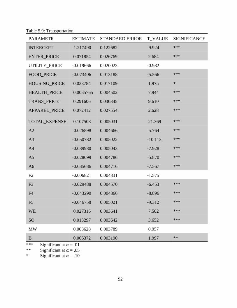
92

Table 5.9: Transportation

PARAMETR ESTIMATE STANDARD ERROR T_VALUE SIGNIFICANCE

INTERCEPT -1.217490 0.122682 -9.924 ***

ENTER_PRICE 0.071854 0.026769 2.684 ***

UTILITY_PRICE -0.019666 0.020023 -0.982

FOOD_PRICE -0.073406 0.013188 -5.566 ***

HOUSING_PRICE 0.033784 0.017109 1.975 *

HEALTH_PRICE 0.0035765 0.004502 7.944 ***

TRANS_PRICE 0.291606 0.030345 9.610 ***

APPAREL_PRICE 0.072412 0.027554 2.628 ***

TOTAL_EXPENSE 0.107508 0.005031 21.369 ***

A2 -0.026898 0.004666 -5.764 ***

A3 -0.050782 0.005022 -10.113 ***

A4 -0.039980 0.005043 -7.928 ***

A5 -0.028099 0.004786 -5.870 ***

A6 -0.035686 0.004716 -7.567 ***

F2 -0.006821 0.004331 -1.575

F3 -0.029488 0.004570 -6.453 ***

F4 -0.043290 0.004866 -8.896 ***

F5 -0.046758 0.005021 -9.312 ***

WE 0.027316 0.003641 7.502 ***

SO 0.013297 0.003642 3.652 ***

MW 0.003628 0.003789 0.957

B 0.006372 0.003190 1.997 **

*** Significant at � = .01** Significant at � = .05* Significant at � = .10

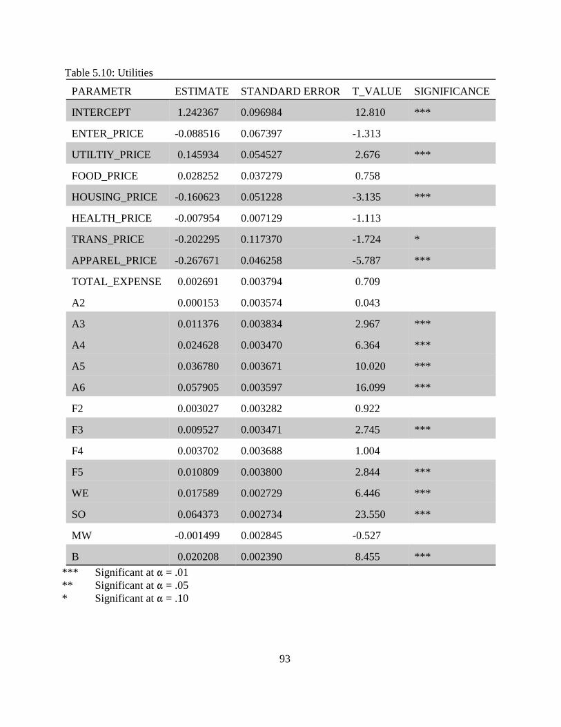
93

Table 5.10: Utilities

PARAMETR ESTIMATE STANDARD ERROR T_VALUE SIGNIFICANCE

INTERCEPT 1.242367 0.096984 12.810 ***

ENTER_PRICE -0.088516 0.067397 -1.313

UTILTIY_PRICE 0.145934 0.054527 2.676 ***

FOOD_PRICE 0.028252 0.037279 0.758

HOUSING_PRICE -0.160623 0.051228 -3.135 ***

HEALTH_PRICE -0.007954 0.007129 -1.113

TRANS_PRICE -0.202295 0.117370 -1.724 *

APPAREL_PRICE -0.267671 0.046258 -5.787 ***

TOTAL_EXPENSE 0.002691 0.003794 0.709

A2 0.000153 0.003574 0.043

A3 0.011376 0.003834 2.967 ***

A4 0.024628 0.003470 6.364 ***

A5 0.036780 0.003671 10.020 ***

A6 0.057905 0.003597 16.099 ***

F2 0.003027 0.003282 0.922

F3 0.009527 0.003471 2.745 ***

F4 0.003702 0.003688 1.004

F5 0.010809 0.003800 2.844 ***

WE 0.017589 0.002729 6.446 ***

SO 0.064373 0.002734 23.550 ***

MW -0.001499 0.002845 -0.527

B 0.020208 0.002390 8.455 ***

*** Significant at � = .01** Significant at � = .05* Significant at � = .10

94

5.4.1 The Impacts of the Age of the Head of the Household

There is a clear difference and pattern in the allocation of resources for the consumption of food

and beverages based on the age of the head of the family. It appears that as the age increases the

expenditure share for food also increases. Expenditure on housing increases at the earlier ages of the

head of the household. One reason for the increase on the share of expenditure on housing might be that

expenditure on housing is considered as a long term investment. People tend to make major investment

decisions in their earlier age. The budget share for apparel generally decreases as age increases and it

is significant at 99%. It is reasonable to say that people allocate more for entertainment and leisure

services during their prime age. The results indicate that the older the head of the household the less the

budget share for entertainment. As people get older their health the state of their health deteriorates and

more is allocated towards health care and health related expenditures. This fact is supported by this

result at 99% level of confidence. While the share of budget for transportation decreases as age

increases, on the contrary the expenditure on utilities increases. The summary of the effects of the age

of the head of the household on the share of expenditure for food is illustrated in Table 5.11.

5.4.2 The Impact of the Size of Household

It appears that as age and family size increase the expenditure shares for food and beverages also

increases. The more the number of people in a household the more food consumed causing an increase

in the share of expenditure for food. The effect of the size of household has a positive effect on goods

and services which are considered basic necessities; goods such as food, health and utilities. The margin

of expenditure decreases for housing, apparel, entertainment, and transportation and the size of the

household increases. The priorities of household consumption are reflected in the amount of resources

allocated for certain commodities and services as the size of the household grows. Table 5.12 just

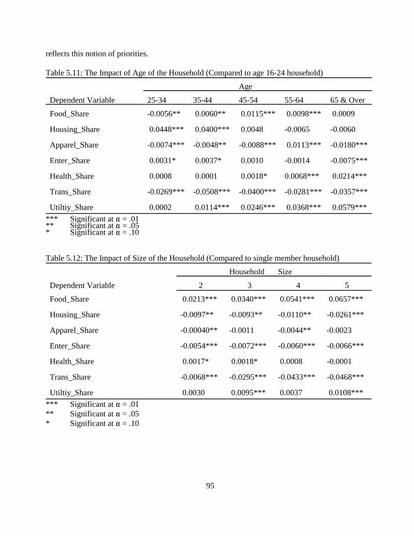
95

reflects this notion of priorities.

Table 5.11: The Impact of Age of the Household (Compared to age 16-24 household)

Age

Dependent Variable 25-34 35-44 45-54 55-64 65 & Over

Food_Share -0.0056** 0.0060** 0.0115*** 0.0098*** 0.0009

Housing_Share 0.0448*** 0.0400*** 0.0048 -0.0065 -0.0060

Apparel_Share -0.0074*** -0.0048** -0.0088*** 0.0113*** -0.0180***

Enter_Share 0.0031* 0.0037* 0.0010 -0.0014 -0.0075***

Health_Share 0.0008 0.0001 0.0018* 0.0068*** 0.0214***

Trans_Share -0.0269*** -0.0508*** -0.0400*** -0.0281*** -0.0357***

Utiltiy_Share 0.0002 0.0114*** 0.0246*** 0.0368*** 0.0579***

*** Significant at � = .01** Significant at � = .05* Significant at � = .10

Table 5.12: The Impact of Size of the Household (Compared to single member household)

Household Size

Dependent Variable 2 3 4 5

Food_Share 0.0213*** 0.0340*** 0.0541*** 0.0657***

Housing_Share -0.0097** -0.0093** -0.0110** -0.0261***

Apparel_Share -0.00040** -0.0011 -0.0044** -0.0023

Enter_Share -0.0054*** -0.0072*** -0.0060*** -0.0066***

Health_Share 0.0017* 0.0018* 0.0008 -0.0001

Trans_Share -0.0068*** -0.0295*** -0.0433*** -0.0468***

Utiltiy_Share 0.0030 0.0095*** 0.0037 0.0108***

*** Significant at � = .01** Significant at � = .05* Significant at � = .10

96

5.4.3 The Impacts of Geographic Location

Geographic location of residence of a household has an effect on the share of expenditure

allocated for the consumption of goods and services. Households living in the east tend to allocate more

for food and beverages than those living in the west, south, and midwest. Households residing in the

southern geographic regions of the country allocate relatively less resources to those living in the

northeast. The Western region residents allocate marginally more on apparel, entertainment,

transportation and utilities while the south spends more on health, transportation, utilities, and less on

apparel, entertainment. Households in the midwestern geographic region spend relatively less on food,

apparel, health and utilities while more is allocated for housing, entertainment, and transportation. Table

5.13 illustrates the relationship and the level of significance.

Table 5.13: Impacts of Geographic Location of a Household (Compared to the Northeast)

Geographic Location

Dependent Variable West South Midwest

Food_Share -0.0222*** -0.0325*** -0.0163***

Housing_Share -0.0240*** -0.0353*** 0.0161

Apparel_Share 0.0005 -0.0059*** -0.0052***

Enter_Share 0.0002 -0.0033** 0.0064***

Health_Share -0.0014* 0.0008 -0.0032***

Trans_Share 0.0273*** 0.0133*** 0.0036

Utiltiy_Share 0.00176*** 0.0644*** -0.0015

*** Significant at � = .01** Significant at � = .05* Significant at � = .10

97

5.4.4 The Impacts of Race

The regression coefficients for the dummy variable race are all statistically significant, indicating

that share of income spent on the different categories vary significantly between white and black

households. Households with a black head of household spend smallest shares of their incomes on

food, housing, health and entertainment, but larger shares on clothing, transportation and utilities.

People whose income is critically small usually receive government assistance in the form of food

stamps, housing rent subsidies and health care services. If blacks allocate less on food, housing and

health care it could be possible that substantial part of their expenditure is covered by public assistance

programs. The assistance received from the public program would free some of these resources,

enabling them to increase the budget shares for apparel, transportation and utilities. Table 5.14

illustrates this relationship with the degree of statistical significance level.

Table 5.14: The Impact of Race (Compared to white)

Dependent Variable Black

Food_Share -0.0185***

Housing_Share -0.0005*

Apparel_Share 0.0094***

Enter_Share -0.0126***

Health_Share -0.0018***

Trans_Share 0.0064**

Utiltiy_Share 0.0202***

*** Significant at � = .01** Significant at � = .05* Significant at � = .10

98

5.4.5 Total Expenditure

Table 5.15 shows the relation between expenditure and budget shares for varius types of goods

and services. The interpretation has to be handled with greater care, because expenditures in this case

does not replace income. To some degree expenditures may indicate whether the good or service is

normal or superior. Most goods and services classified as basic necessity goods are normal goods. Such

goods and services are indicated by negative signs, where as the budget shares for transportation,

utilities and apparel increase as expenditures increase. This is a very interesting finding for

understanding the consumption patterns of households.

The impact of demographic characteristics has a wide range of implications for both private

organizations, which have a business interest in understanding the distribution of expenditure patterns

of households, and government agencies which help determine the economic well-being of the nation

and make long term and short term planning to improve the welfare of especially the less fortunate.

Table 5.15: The Impact of Total Expenditure on Share of Expenditures

Dependent Variable Total Expenditure

Food_Share -0.0659***

Housing_Share -0.0312***

Apparel_Share 0.0046**

Enter_Share -0.0007

Health_Share -0.0068***

Trans_Share 0.1075***

Utiltiy_Share 0.0027

*** Significant at � = .01** Significant at � = .05* Significant at � = .10

99

G �

2 cov(X, F)m

(6.1)

CHAPTER 6: INEQUALITY IN HOUSEHOLD CONSUMPTION EXPENDITURES

6.1 Introduction

Following the methodology and formulas laid out in section 3.3 of chapter 3, this chapter is an

analysis of inequality in the household consumption expenditures, where relationships are examined

between various expenditure budget components using the consumer expenditure data from 1980 to

1994. Identifying the impact of marginal changes in expenditures for specific commodities on the

inequality of total expenditures can provide useful information concerning the effect that certain policies,

such as the introduction of percentage commodity taxes and subsidies, may have on the spending

patterns of consumers. Section 6.2 addresses the use of the Gini coefficient and its decomposition. Then,

the results are presented and discussed in section 6.3. Conclusions are presented in section 6.4.

6.2 The Gini Coefficient and Its Decomposition

The overall Gini coefficient is applied to produce an estimate of the inequality in the distribution

of total household consumption expenditure over the population. Following the derivation by Lerman

and Yitzhaki (1984), we can express the formula for the Gini coefficient as:

This formula is expressed in terms of the covariance between total expenditures (X) and the

commutative distribution of X (F), and the mean of X (m). The lower the value of the Gini, the lower

the inequality in the distribution of expenditures; zero represents absolute equality. The overall Gini is

decomposed by expenditure budget components as: Let x1, .....,xk represent the level of expenditure for

budget components. The Gini coefficient for component k is:

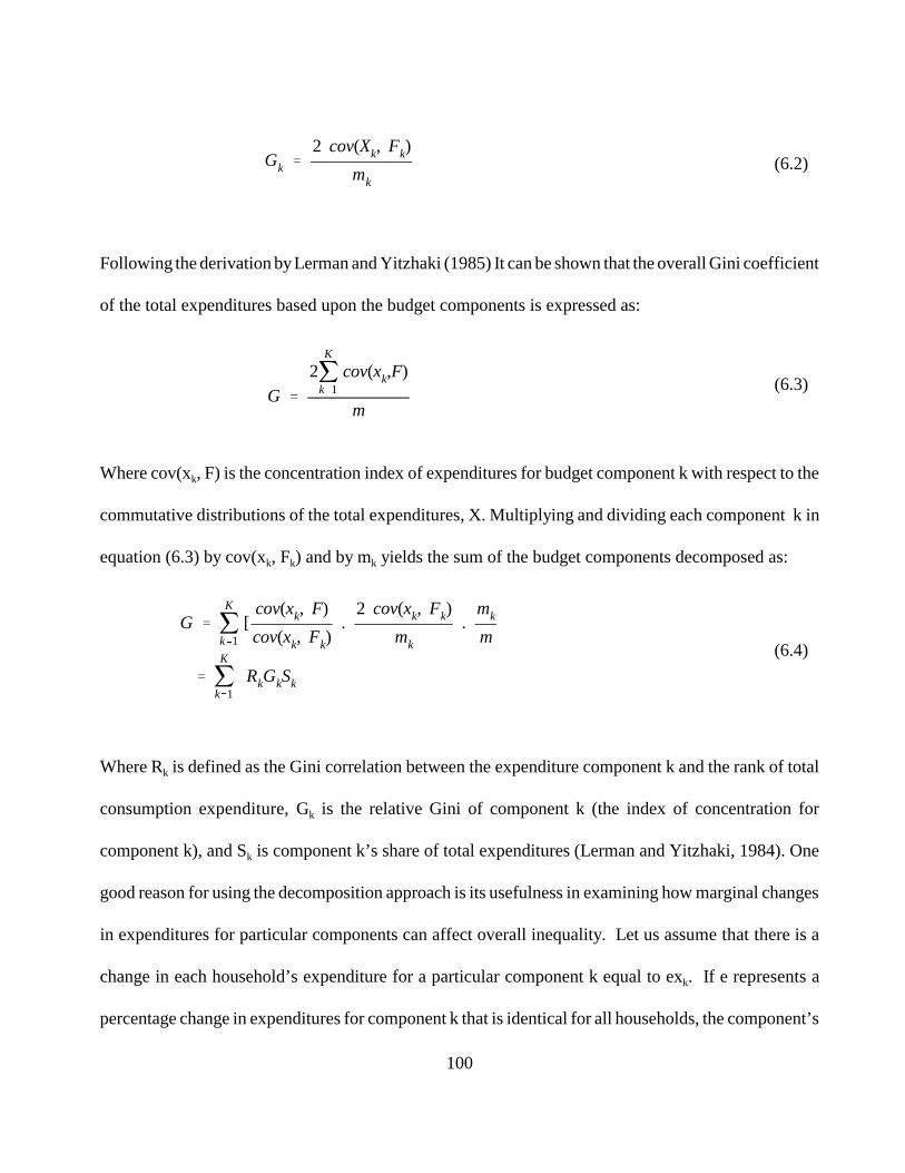
100

Gk �

2 cov(Xk, Fk)

mk

(6.2)

G �

2�K

k�1cov(xk,F)

m

(6.3)

G � �K

k�1[

cov(xk, F)

cov(xk, Fk).

2 cov(xk, Fk)

mk

.mk

m

� �K

k�1RkGkSk

(6.4)

Following the derivation by Lerman and Yitzhaki (1985) It can be shown that the overall Gini coefficient

of the total expenditures based upon the budget components is expressed as:

Where cov(xk, F) is the concentration index of expenditures for budget component k with respect to the

commutative distributions of the total expenditures, X. Multiplying and dividing each component k in

equation (6.3) by cov(xk, Fk) and by mk yields the sum of the budget components decomposed as:

Where Rk is defined as the Gini correlation between the expenditure component k and the rank of total

consumption expenditure, Gk is the relative Gini of component k (the index of concentration for

component k), and Sk is component k’s share of total expenditures (Lerman and Yitzhaki, 1984). One

good reason for using the decomposition approach is its usefulness in examining how marginal changes

in expenditures for particular components can affect overall inequality. Let us assume that there is a

change in each household’s expenditure for a particular component k equal to exk. If e represents a

percentage change in expenditures for component k that is identical for all households, the component’s

101

�G�ek

G�

RkGSkk

G� Sk

(6.5)

marginal effect relative to the overall Gini coefficient can be represented as (Garner, 1989):

The interpretation of the above equation is that the percentage change in the overall Gini, caused by a

small change in a commodity expenditure is equal to the commodity’s contribution to overall inequality

(named as Ik in the results column). The overall Gini would remain unchanged if all components are

multiplied by e (Lerman and Yitzhaki, 1985). The result from equation (8.5) may help to determine the

distributional effect of imposing a commodity percentage tax or raising the tax rate, where the tax leads

to a small change in commodity expenditures. When the relative marginal effect is positive, taxing a

commodity would decrease overall inequality (Garner, 1993). Such a tax would be progressive since

it affects the rich more than it affects the poor at the margin. When the relative marginal effect is

negative, taxing the commodity would increase inequality, as would be expected from a tax which is

regressive (Garner, 1993).

The above method and approach is implemented using total expenditures which are

disaggregated into eight categories: food and beverages, housing, apparel, entertainment, health care,

transportation, utilities, and personal care and education. Also, inequality in the distribution of

expenditures is measured within each of the age categories of 16-24, 25-34, 35-44, 45-54, 55-64, and

65 and above, as well as within each of the two racial subgroups.

As described in chapter 6, microlevel data from the U.S. Consumer Expenditure Interview

Survey for the years 1980-1994 are analyzed. Table 6.1 gives descriptions of the measures of inequality.

102

Table 6.1: Descriptions of Measures of Inequality

NAME DESCRIPTION

Ck CONTRIBUTION TO TOTAL INEQUALITY FOR COMPONENT K

Rk CORRELATION TO RANK OF TOTAL EXPENDITURE

G OVERALL Gini COEFFICIENT FOR THE WHOLE POPULATION

Gk Gini OF COMPONENT k

Sk EXPENDITURE SHARE FOR COMPONENT K

Ik SHARE EXPENDITURE INEQUALITY FOR COMPONENT K

Ik/Sk RELATIVE EXPENDITURE INEQUALITY FOR COMPONENT K

Ik - Sk RELATIVE MARGINAL EFFECT FOR COMPONENT K

6.3 Results and Discussions

The expenditure inequality effects by budget component are presented in tables 6.3 - 6.17 for the

years 1980 - 1994. In the discussion of the results, the focus is mainly on the result for the year 1980.

There are two reasons for doing this: first, the differences in the Gini inequality in consumption

expenditures, among the years from 1980 to 1994 is small. There are no clear patterns or trends of

inequality from year to year. Second, by showing how to interpret the results for one year, the reader

can make his/her interpretations for the rest, using the same approach.

The first column in the table 6.3 presents the contribution of each budget component to total

inequality as identified by Ck. This measure is the product of three terms: the Gini correlation between

the budget component and the rank of total expenditures (Rk), the component’s Gini (Gk), and its share

of total expenditures (Sk). The higher the value of each factor, the greater is the contribution of the

budget component to total inequality. The proportion of inequality to total expenditures attributable to

each commodity is given in column five as Ik, and is defined as Ck divided by G. Relative effects are

presented in columns six and seven.

103

The overall Gini based on the total annual consumption expenditure for the last 15 year is

between 0.195 the lowest and 0.281 the highest. The overall Gini ratio (from the total row Table 6.3)

of household expenditure inequality for the year 1980 calculated as 0.214. The Gini coefficient for total

expenditure inequality is graphically illustrated in figure 6.1. These numbers indicate a relatively low

household inequality in expenditures. Nelson (1994) calculated the Gini for family income inequality

as 0.365 (see table 6.19) and a study by Garner (1993) calculated the Gini for income and expenditure

inequalities for the 1987 as 0.435 and 0.330 respectively. In both cases the differences between

expenditure and income inequalities is around 0.100. The smaller expenditure inequality can be

attributed to the consumption and expenditure patterns based on the permanent income theory.

Expenditures in one year do not depend only on the income of that year. People with reduced incomes

tend to spend from their savings or they may borrow and spend against their expected future income.

Also, there are numerous government and community based programs which provide food, energy,

medical even cash assistance to millions who are in the lower income brackets. Above all, the major

factor for the difference in inequality between consumption and expenditure is that in normal years

people usually do not consume everything they earn, some of it goes to savings and investment. As a

result of the inequality in consumption is smaller than inequality in income. In general, the overall Gini

for expenditure inequality has not changed much through the years from 1980 to 1994.

Expenditures shares for food and beverages, housing, and transportation account for over 50%

of the inequality in total expenditures. Their share of total expenditures is about the same as their share

of inequality. Housing and transportation have the highest shares of expenditure inequality as

represented by Ik, 0.229 and 0.234, respectively for 1980.

A high Gini correlation indicates higher total expenditures with greater spending on the

104

individual commodity. Expenditures for food, housing, and transportation are more highly correlated

with the rank of total expenditures. High Gk’s are an indication that there are differences in consumption

expenditures. The results in general imply that there are relatively large differences in spending for

health care, entertainment, utilities, transportation, and personal care and education. Expenditures for

food and beverages, apparel, and housing are fairly equally distributed, relative to expenditures for other

commodities.

Relative expenditure inequality (Ik/ Sk) measures the inequality for components as a percentage

of expenditure shares. These estimates are calculated as the ratio of the proportional contribution to the

share of total expenditures. Expenditures for food, housing, entertainment, transportation, and personal

care and education contribute more to the inequality in total expenditures than they contribute to total

expenditures in terms of their shares.

Changes in expenditures which would lead to reductions in inequality are associated with

expenditures categories for which the expenditure shares are greater than the shares of inequality. The

direction of the relative marginal relationship indicates the effect at the margin of an increase in

expenditures for a component for overall inequality (Ik - Sk). These results reveal that increases in

expenditures in 1980 for food and beverages, housing, apparel, entertainment, health care, utilities, and

personal care and education would have decreased overall inequality in total expenditures, holding all

else constant. Table 6.2 illustrates the signs for the overall inequality (Ik - Sk) for all commodities for

the year between 1980-1994. Food, apparel. And housing expenditures had negative signs in all fifteen

years, while transportation had a positive sign in 13 of the 15 years, entertainment was positive about

half the time. The other categories all had 13 to 14 years with negative signs. From a policy perspective,

increases in overall inequality could be achieved by reducing taxes on these goods and services or by

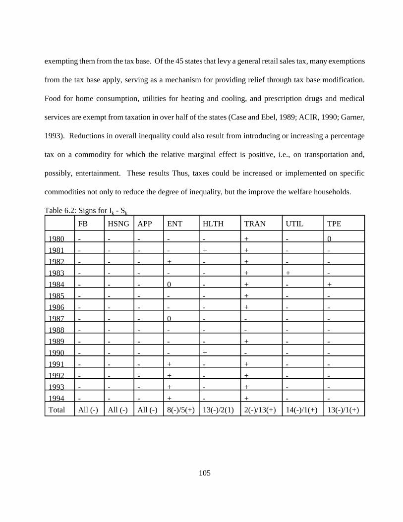
105

exempting them from the tax base. Of the 45 states that levy a general retail sales tax, many exemptions

from the tax base apply, serving as a mechanism for providing relief through tax base modification.

Food for home consumption, utilities for heating and cooling, and prescription drugs and medical

services are exempt from taxation in over half of the states (Case and Ebel, 1989; ACIR, 1990; Garner,

1993). Reductions in overall inequality could also result from introducing or increasing a percentage

tax on a commodity for which the relative marginal effect is positive, i.e., on transportation and,

possibly, entertainment. These results Thus, taxes could be increased or implemented on specific

commodities not only to reduce the degree of inequality, but the improve the welfare households.

Table 6.2: Signs for Ik - Sk

FB HSNG APP ENT HLTH TRAN UTIL TPE

1980 - - - - - + - 0

1981 - - - - + + - -

1982 - - - + - + - -

1983 - - - - - + + -

1984 - - - 0 - + - +

1985 - - - - - + - -

1986 - - - - - + - -

1987 - - - 0 - - - -

1988 - - - - - - - -

1989 - - - - - + - -

1990 - - - - + - - -

1991 - - - + - + - -

1992 - - - + - + - -

1993 - - - + - + - -

1994 - - - + - + - -

Total All (-) All (-) All (-) 8(-)/5(+) 13(-)/2(1) 2(-)/13(+) 14(-)/1(+) 13(-)/1(+)

106

Inequality in expenditures by age is computed and presented in table 6.18. The categories are

made up of ages 16-24, 25-34, 35-44, 45-54, 55-64, and 65 and over. The overall Gin is within each

group are extremely low (all under 0.08) implying that expenditures are fairly equal within each group.

Table 6.19 illustrates expenditure inequality based on race: black and white. Again, the overall Gini is

for both races are relatively low, and are similar to those for all consumers. The highest Gini for whites

is 0.284 in 1988 and the lowest 0.176 in 1981. For blacks the highest Gini is 0.244 in 1984 and the

lowest 0.166 in 1991. These results do not, however, indicate that expenditures are equal between the

races; this was not measured. Table 6.20 is included to show the difference between the income and

expenditure inequalities.

6.4 Conclusion

The focus of this chapter has been to measure inequality in the distribution of consumption

expenditures across consumer units in general, consumers grouped based on age, and consumers

categorized by race. The overall Gini coefficient and other forms of inequality measures were produced

as estimates to shed light on the state of consumer expenditures for the years 1980-1994. These results

reveal very important information which can be used in the formulation of policy initiatives. The

inequality of household consumption expenditures in particular commodity categories suggests possible

targets for additional consumption taxation introduced to reduce the social impact created by other

economic inequalities.

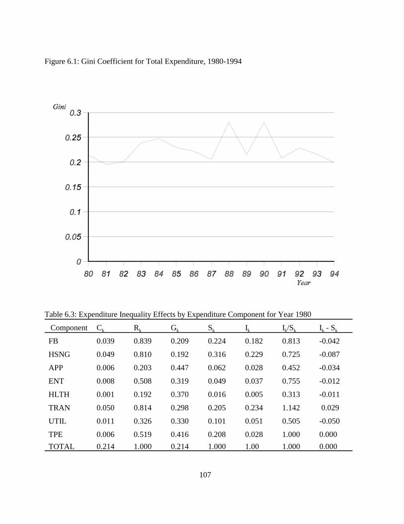
107

Figure 6.1: Gini Coefficient for Total Expenditure, 1980-1994

Table 6.3: Expenditure Inequality Effects by Expenditure Component for Year 1980

Component Ck Rk Gk Sk Ik Ik/Sk Ik - Sk

FB 0.039 0.839 0.209 0.224 0.182 0.813 -0.042

HSNG 0.049 0.810 0.192 0.316 0.229 0.725 -0.087

APP 0.006 0.203 0.447 0.062 0.028 0.452 -0.034

ENT 0.008 0.508 0.319 0.049 0.037 0.755 -0.012

HLTH 0.001 0.192 0.370 0.016 0.005 0.313 -0.011

TRAN 0.050 0.814 0.298 0.205 0.234 1.142 0.029

UTIL 0.011 0.326 0.330 0.101 0.051 0.505 -0.050

TPE 0.006 0.519 0.416 0.208 0.028 1.000 0.000

TOTAL 0.214 1.000 0.214 1.000 1.00 1.000 0.000

108

Table 6.4: Expenditure Inequality Effects by Expenditure Component for Year 1981

Component Ck Rk Gk Sk Ik Ik/Sk Ik - Sk

FB 0.038 0.813 0.222 0.211 0.195 0.924 -0.016

HSNG 0.053 0.770 0.211 0.323 0.272 0.842 -0.051

APP 0.012 0.740 0.277 0.063 0.062 0.984 -0.001

ENT 0.009 0.563 0.328 0.048 0.046 0.958 -0.002

HLTH 0.010 0.218 0.371 0.017 0.051 3.000 0.034

TRAN 0.047 0.784 0.293 0.204 0.241 1.181 0.037

UTIL 0.017 0.620 0.254 0.106 0.088 0.830 -0.018

TPE 0.005 0.434 0.420 0.028 0.026 0.929 -0.002

TOTAL 0.195 1.000 0.195 1.000 1.000 1.000 0.000

Table 6.5: Expenditure Inequality Effects by Expenditure Component for Year 1982

Component Ck Rk Gk Sk Ik Ik/Sk Ik - Sk

FB 0.036 0.860 0.220 0.192 0.180 0.938 -0.012

HSNG 0.058 0.858 0.205 0.333 0.290 0.871 -0.043

APP 0.012 0.788 0.248 0.061 0.060 0.984 -0.001

ENT 0.011 0.722 0.297 0.049 0.055 1.120 0.006

HLTH 0.001 0.097 0.303 0.017 0.005 0.294 -0.012

TRAN 0.046 0.776 0.295 0.201 0.230 1.144 0.029

UTIL 0.016 0.534 0.264 0.114 0.080 0.702 -0.034

TPE 0.006 0.385 0.432 0.034 0.030 0.882 -0.004

TOTAL 0.200 1.000 0.200 1.000 1.000 1.000 0.000

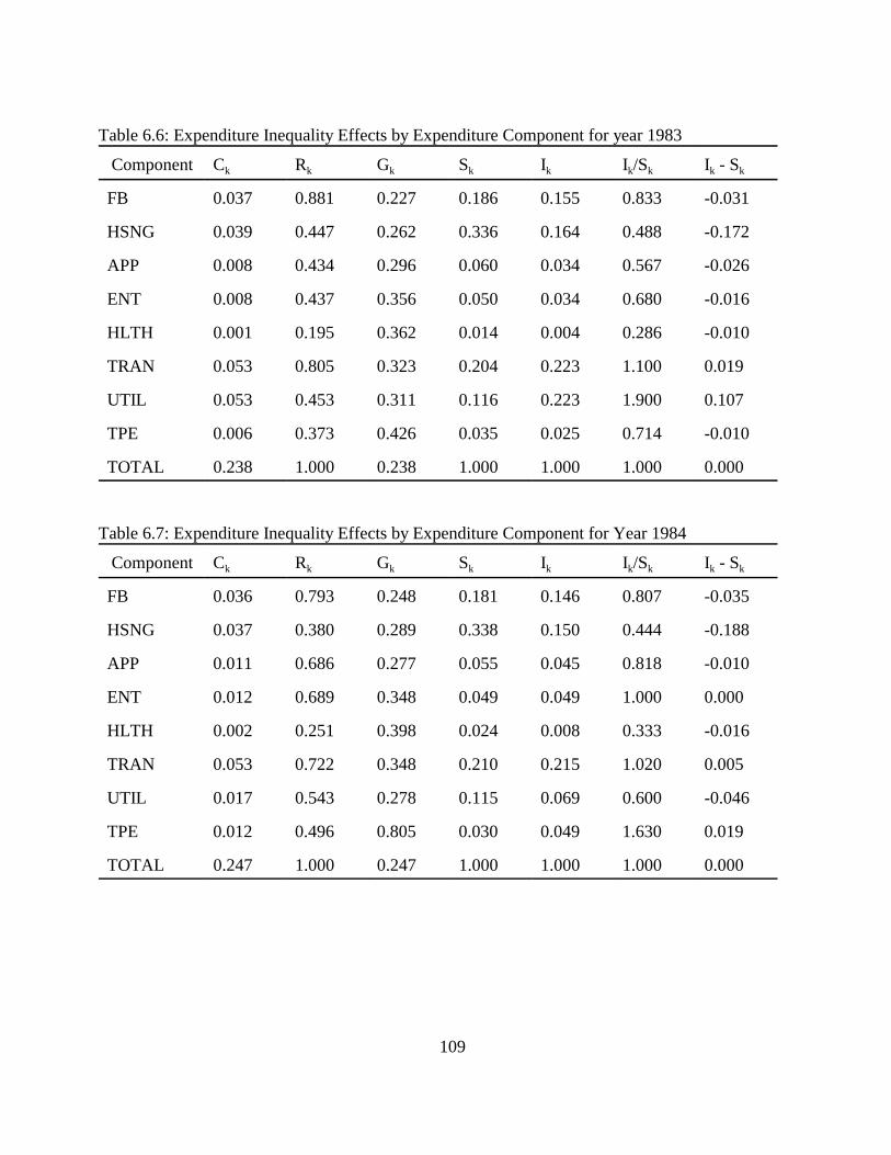
109

Table 6.6: Expenditure Inequality Effects by Expenditure Component for year 1983

Component Ck Rk Gk Sk Ik Ik/Sk Ik - Sk

FB 0.037 0.881 0.227 0.186 0.155 0.833 -0.031

HSNG 0.039 0.447 0.262 0.336 0.164 0.488 -0.172

APP 0.008 0.434 0.296 0.060 0.034 0.567 -0.026

ENT 0.008 0.437 0.356 0.050 0.034 0.680 -0.016

HLTH 0.001 0.195 0.362 0.014 0.004 0.286 -0.010

TRAN 0.053 0.805 0.323 0.204 0.223 1.100 0.019

UTIL 0.053 0.453 0.311 0.116 0.223 1.900 0.107

TPE 0.006 0.373 0.426 0.035 0.025 0.714 -0.010

TOTAL 0.238 1.000 0.238 1.000 1.000 1.000 0.000

Table 6.7: Expenditure Inequality Effects by Expenditure Component for Year 1984

Component Ck Rk Gk Sk Ik Ik/Sk Ik - Sk

FB 0.036 0.793 0.248 0.181 0.146 0.807 -0.035

HSNG 0.037 0.380 0.289 0.338 0.150 0.444 -0.188

APP 0.011 0.686 0.277 0.055 0.045 0.818 -0.010

ENT 0.012 0.689 0.348 0.049 0.049 1.000 0.000

HLTH 0.002 0.251 0.398 0.024 0.008 0.333 -0.016

TRAN 0.053 0.722 0.348 0.210 0.215 1.020 0.005

UTIL 0.017 0.543 0.278 0.115 0.069 0.600 -0.046

TPE 0.012 0.496 0.805 0.030 0.049 1.630 0.019

TOTAL 0.247 1.000 0.247 1.000 1.000 1.000 0.000

110

Table 6.8: Expenditure Inequality Effects by Expenditure Component for Year 1985

Component Ck Rk Gk Sk Ik Ik/Sk Ik - Sk

FB 0.036 0.873 0.230 0.180 0.157 0.872 -0.023

HSNG 0.069 0.865 0.238 0.335 0.301 0.899 –0.034

APP 0.012 0.734 0.275 0.061 0.052 0.852 -0.009

ENT 0.010 0.575 0.369 0.051 0.044 0.863 -0.047

HLTH 0.002 0.189 0.452 0.024 0.009 0.375 -0.015

TRAN 0.058 0.813 0.350 0.202 0.253 1.252 0.051

UTIL 0.018 0.549 0.290 0.112 0.079 0.705 -0.033

TPE 0.007 0.357 0.463 0.034 0.020 0.588 -0.014

TOTAL 0.229 1.000 0.229 1.000 1.000 1.000 0.000

Table 6.9: Expenditure Inequality Effects by Expenditure Component for Year 1986

Component Ck Rk Gk Sk Ik Ik/Sk Ik - Sk

FB 0.033 0.841 0.223 0.176 0.149 0.847 -0.027

HSNG 0.065 0.861 0.227 0.333 0.293 0.880 -0.040

APP 0.010 0.757 0.251 0.059 0.045 0.763 -0.014

ENT 0.009 0.473 0.347 0.053 0.041 0.774 -0.012

HLTH 0.002 0.268 0.338 0.021 0.006 0.286 -0.015

TRAN 0.058 0.838 0.332 0.208 0.261 1.260 0.053

UTIL 0.020 0.556 0.297 0.121 0.090 0.744 -0.031

TPE 0.006 0.462 0.427 0.030 0.027 0.223 -0.003

TOTAL 0.222 1.000 0.222 1.000 1.000 1.000 0.000

111

Table 6.10: Expenditure Inequality Effects by Expenditure Component for Year 1987

Component Ck Rk Gk Sk Ik Ik/Sk Ik - Sk

FB 0.032 0858 0212 0.175 0.156 0.891 -0.019

HSNG 0.049 0.618 0.235 0.335 0.239 0.713 -0.096

APP 0.010 0.620 0.246 0.063 0.049 0.778 -0.014

ENT 0.011 0.665 0.295 0.054 0.054 1.000 0.000

HLTH 0.002 0.267 0.313 0.021 0.010 0.476 -0.011

TRAN 0.048 0.789 0.298 0.205 0.234 1.142 -0.029

UTIL 0.020 0.659 0.259 0.114 0.098 0.860 -0.016

TPE 0.005 0.421 0.385 0.032 0.024 0.750 -0.008

TOTAL 0.205 1.000 0.205 1.000 1.000 1.000 0.000

Table 6.11: Expenditure Inequality Effects by Expenditure Component for Year 1988

Component Ck Rk Gk Sk Ik Ik/Sk Ik - Sk

FB 0.031 0.782 0.224 0.179 0.110 0.615 -0.069

HSNG 0.014 0.390 0.307 0.339 0.146 0431 -0.193

APP 0.010 0.677 0.268 0.057 0.036 0.632 -0.021

ENT 0.011 0.609 0.349 0.052 0.039 0.750 -0.013

HLTH 0.002 0.225 0.338 0.023 0.007 0.304 -0.016

TRAN 0.023 0.245 0.464 0.205 0.082 0.400 -0.123

UTIL 0.017 0.432 0.332 0.117 0.061 0.521 -0.560

TPE 0.005 0.475 0.392 0.028 0.018 0.643 -0.010

TOTAL 0.281 1.000 0.281 1.000 1.000 1.000 0.0000

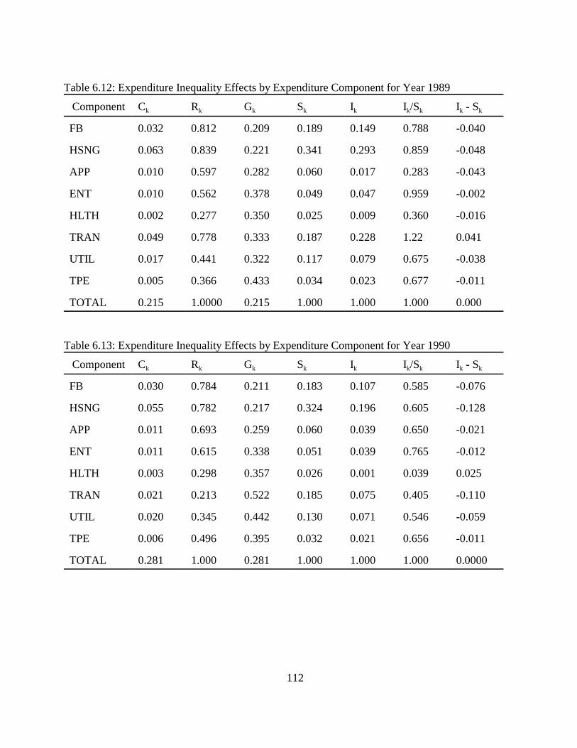
112

Table 6.12: Expenditure Inequality Effects by Expenditure Component for Year 1989

Component Ck Rk Gk Sk Ik Ik/Sk Ik - Sk

FB 0.032 0.812 0.209 0.189 0.149 0.788 -0.040

HSNG 0.063 0.839 0.221 0.341 0.293 0.859 -0.048

APP 0.010 0.597 0.282 0.060 0.017 0.283 -0.043

ENT 0.010 0.562 0.378 0.049 0.047 0.959 -0.002

HLTH 0.002 0.277 0.350 0.025 0.009 0.360 -0.016

TRAN 0.049 0.778 0.333 0.187 0.228 1.22 0.041

UTIL 0.017 0.441 0.322 0.117 0.079 0.675 -0.038

TPE 0.005 0.366 0.433 0.034 0.023 0.677 -0.011

TOTAL 0.215 1.0000 0.215 1.000 1.000 1.000 0.000

Table 6.13: Expenditure Inequality Effects by Expenditure Component for Year 1990

Component Ck Rk Gk Sk Ik Ik/Sk Ik - Sk

FB 0.030 0.784 0.211 0.183 0.107 0.585 -0.076

HSNG 0.055 0.782 0.217 0.324 0.196 0.605 -0.128

APP 0.011 0.693 0.259 0.060 0.039 0.650 -0.021

ENT 0.011 0.615 0.338 0.051 0.039 0.765 -0.012

HLTH 0.003 0.298 0.357 0.026 0.001 0.039 0.025

TRAN 0.021 0.213 0.522 0.185 0.075 0.405 -0.110

UTIL 0.020 0.345 0.442 0.130 0.071 0.546 -0.059

TPE 0.006 0.496 0.395 0.032 0.021 0.656 -0.011

TOTAL 0.281 1.000 0.281 1.000 1.000 1.000 0.0000

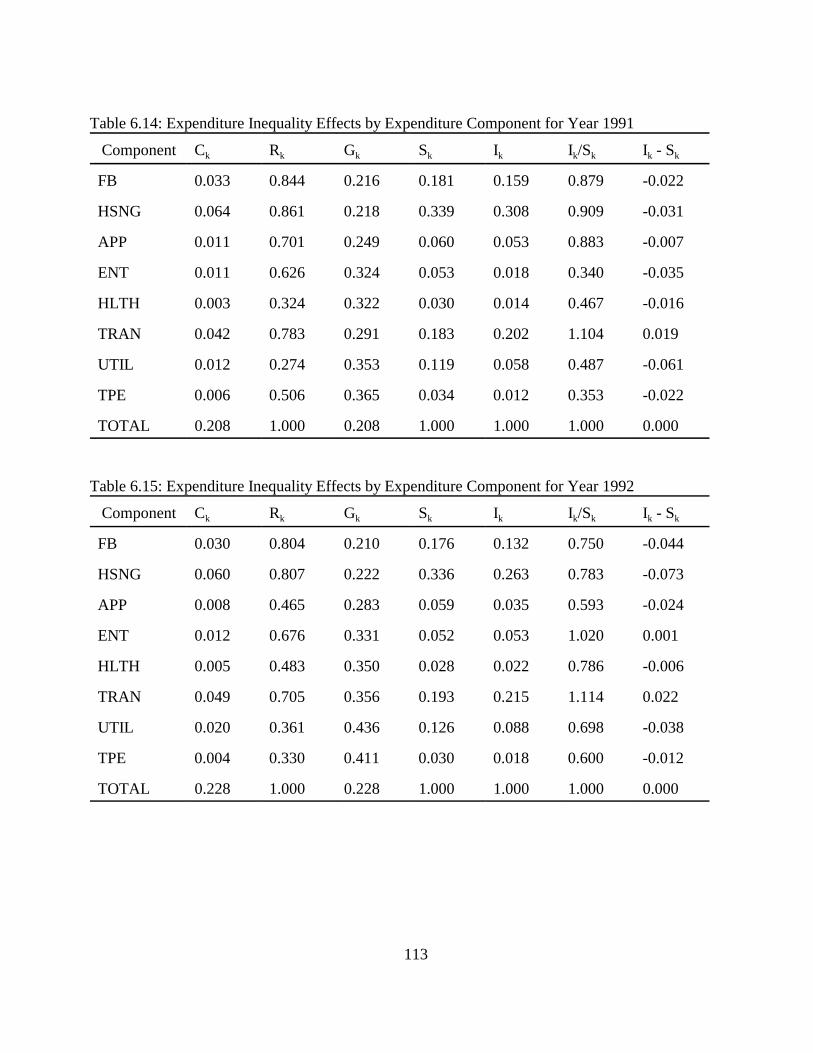
113

Table 6.14: Expenditure Inequality Effects by Expenditure Component for Year 1991

Component Ck Rk Gk Sk Ik Ik/Sk Ik - Sk

FB 0.033 0.844 0.216 0.181 0.159 0.879 -0.022

HSNG 0.064 0.861 0.218 0.339 0.308 0.909 -0.031

APP 0.011 0.701 0.249 0.060 0.053 0.883 -0.007

ENT 0.011 0.626 0.324 0.053 0.018 0.340 -0.035

HLTH 0.003 0.324 0.322 0.030 0.014 0.467 -0.016

TRAN 0.042 0.783 0.291 0.183 0.202 1.104 0.019

UTIL 0.012 0.274 0.353 0.119 0.058 0.487 -0.061

TPE 0.006 0.506 0.365 0.034 0.012 0.353 -0.022

TOTAL 0.208 1.000 0.208 1.000 1.000 1.000 0.000

Table 6.15: Expenditure Inequality Effects by Expenditure Component for Year 1992

Component Ck Rk Gk Sk Ik Ik/Sk Ik - Sk

FB 0.030 0.804 0.210 0.176 0.132 0.750 -0.044

HSNG 0.060 0.807 0.222 0.336 0.263 0.783 -0.073

APP 0.008 0.465 0.283 0.059 0.035 0.593 -0.024

ENT 0.012 0.676 0.331 0.052 0.053 1.020 0.001

HLTH 0.005 0.483 0.350 0.028 0.022 0.786 -0.006

TRAN 0.049 0.705 0.356 0.193 0.215 1.114 0.022

UTIL 0.020 0.361 0.436 0.126 0.088 0.698 -0.038

TPE 0.004 0.330 0.411 0.030 0.018 0.600 -0.012

TOTAL 0.228 1.000 0.228 1.000 1.000 1.000 0.000

114

Table 6.16: Expenditure Inequality Effects by Expenditure Component for Year 1993

Component Ck Rk Gk Sk Ik Ik/Sk Ik - Sk

FB 0.031 0.814 0.216 0.173 0.144 0.832 -0.029

HSNG 0.067 0.835 0.234 0.344 0.310 0.901 -0.034

APP 0.009 0.552 0.273 0.059 0.042 0.712 -0.017

ENT 0.012 0.094 0.335 0.052 0.056 1.08 0.004

HLTH 0.005 0.509 0.324 0.030 0.023 0.767 -0.007

TRAN 0.050 0.773 0.356 0.181 0.232 1.282 0.051

UTIL 0.019 0.474 0.306 0.130 0.088 0.677 -0.042

TPE 0.006 0.483 0.399 0.030 0.028 0.933 -0.002

TOTAL 0.216 1.000 0.216 1.000 1.000 1.000 0.000

Table 6.17: Expenditure Inequality Effects by Expenditure Component for Year 1994

Component Ck Rk Gk Sk Ik Ik/Sk Ik - Sk

FB 0.029 0.809 0.216 0.168 0.146 0.869 -0.022

HSNG 0.059 0.811 0.213 0.343 0.297 0.866 -0.046

APP 0.008 0.604 0.246 0.054 0.040 0.741 -0.014

ENT 0.010 0.732 0.295 0.048 0.050 1.042 0.002

HLTH 0.005 0.547 0.336 0.029 0.025 0.862 -0.004

TRAN 0.043 0.656 0.328 0.201 0.216 1.075 0.015

UTIL 0.021 0.537 0.315 0.125 0.106 0.848 -0.019

TPE 0.005 0.436 0.369 0.033 0.025 0.758 -0.008

TOTAL 0.199 1.000 0.199 1.000 1.000 1.000 0.000

115

Table 6.18: Expenditure Inequality by Age Using the Gini Coefficient.

YEAR 16-24 25-34 35-44 45-54 55-64 >=65

1980 0.035 0.020 0.028 0.041 0.037 0.032

1981 0.022 0.025 0.028 0.034 0.030 0.036

1982 0.022 0.026 0.030 0.033 0.040 0.030

1983 0.025 0.030 0.035 0.036 0.054 0.041

1984 0.033 0.035 0.052 0.036 0.035 0.045

1985 0.032 0.034 0.033 0.032 0.044 0.038

1986 0.025 0.031 0.036 0.036 0.039 0.038

1987 0.023 0.029 0.028 0.033 0.038 0.035

1988 0.026 0.028 0.044 0.052 0.032 0.078

1989 0.023 0.029 0.033 0.037 0.042 0.029

1990 0.026 0.076 0.034 0.033 0.051 0.037

1991 0.020 0.027 0.040 0.034 0.029 0.040

1992 0.025 0.033 0.035 0.043 0.035 0.038

1993 0.021 0.027 0.034 0.038 0.042 0.026

1994 0.021 0.029 0.031 0.034 0.034 0.036

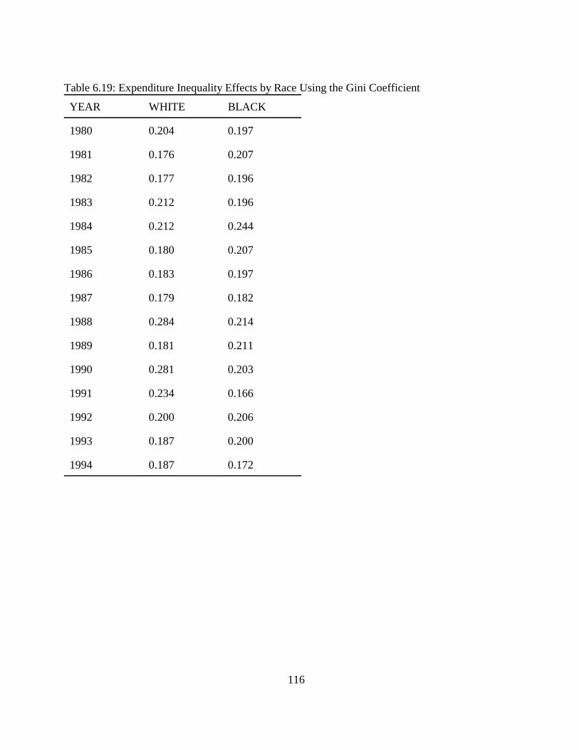
116

Table 6.19: Expenditure Inequality Effects by Race Using the Gini Coefficient

YEAR WHITE BLACK

1980 0.204 0.197

1981 0.176 0.207

1982 0.177 0.196

1983 0.212 0.196

1984 0.212 0.244

1985 0.180 0.207

1986 0.183 0.197

1987 0.179 0.182

1988 0.284 0.214

1989 0.181 0.211

1990 0.281 0.203

1991 0.234 0.166

1992 0.200 0.206

1993 0.187 0.200

1994 0.187 0.172

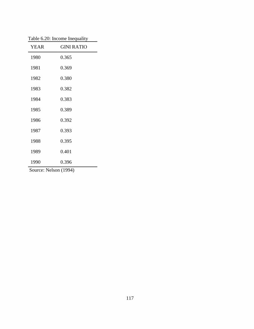
117

Table 6.20: Income Inequality

YEAR GINI RATIO

1980 0.365

1981 0.369

1982 0.380

1983 0.382

1984 0.383

1985 0.389

1986 0.392

1987 0.393

1988 0.395

1989 0.401

1990 0.396

Source: Nelson (1994)

118

CHAPTER 7. SUMMARY AND CONCLUSION

7.1 Background

The measurement of inequality has long concerned writers in the field of personal income

distribution. A casual examination the menu of government programs reveals that distributional

considerations play an important role in the formulation of public policy in the United States. There are

many different expenditures on social insurance and transfer programs that are designed both to provide

a minimal standard of living for the poor as well as reduce the level of inequality, however, there also are

some tax and other policies that increase inequality. There are traditional methods of measuring income

inequality that help to shed light on the situation in the labor market. However, many issues in the

distribution of well-being have remained unanswered.

Using family income as a measure of well-being without taking into account prices and other

characteristics may lead to erroneous conclusions about the general welfare of households. Each

household has its own characteristics in which its consumption and expenditure patterns are a function

of its composition and other demographic factors. A household with five members differs from a

household with two members in its expenditure and consumption patterns, given the same amount of

resources. Using earnings alone to measure welfare ignores the effects of prices and the impacts of

demographic characteristics and may not be a good indicator of welfare disparity.

Economic well-being can be defined in terms of the command individuals or households have

over potential consumption. Official income statistics are produced to reflect the consumption potential

of individuals or families with money income used most frequently to proxy this consumption potential.

However, consumption, rather than income, may be a better indicator of the actual economic welfare of

a household. The value of consumption may be much greater than annually reported income to the extent

119

that households have accumulated savings or accounting losses from businesses, or because they are able

to borrow against future income (Garner, 1993). Thus, one could argue that consumption reflects

material well-being in terms of past, current, and expected future income. How a household allocates its

income across different consumption categories can affect the overall economic well-being of households

differently. Identifying the effects of demographic characteristics of a household, the impact of marginal

changes in different expenditures on the inequality of total expenditures can provide useful information,

especially for policy makers.

This study addresses two important issues related to measures of economic well-being. The first

part analyzes the impacts of demographic characteristics on the expenditure patterns of households using

an econometric approach. In this model a system of individual demand functions depend of the prices

faced by all households, total expenditures, and attributes such as demographic characteristics that vary

among households. There are four categories of demographic characteristics included in the model.

These characteristics are represented with a dummy variable valued 1 if true or 0 if false. Consumer

expenditures are divided among eight commodity groups and with the share of expenditures of each used

as the dependent variable.

1. Food and Beverages: Expenditures on food and beverages at home and away from home.

2. Housing: Expenditures on housing and housing services.

3.Apparel: Expenditures on clothing

4. Entertainment: Expenditures on all forms entertainment.

5. Heath: Expenditures on health and health services.

6. Transportation: Expenditures on transportation.

7. Utilities: Expenditures on utilities.

120

8. Personal care and education: Expenditures on personal care and education.

The following demographic characteristics are employed as attributes of individual households; to avoid

perfect collinearity the first dummy variable from each group is omitted.

1. Family size: 1, 2, 3, 4, 5 persons.

2.Age of the head of the family: 16-24, 25-34, 35-44, 45-54, 55-64, 65 or greater.

3. Region of residence: Northeast, West, Midwest, South.

4. Race: White, black.

The logarithmic indirect translog functional form is used in the application of the model.

Aggregate demand functions are obtained by summing over individual functions. Yearly consumer

expenditure data for the years 1980-1994 are used in this analysis and combined cross section-time series

are used in the econometric estimation..

The second part of this study evaluates inequality in consumption expenditures across consumer

units including inequality within time, age and race categories. Gini coefficients are calculated for the

total population sample and for demographic subgroups for the years 1980-1994. In addition, the Gini

coefficients are decomposed by budget components, using the Lerman-Yitzhaki covariance method, to

examine the effects of changes in expenditures on overall inequality. The same data set, the consumer

expenditure survey, used in the econometric analysis is also used in estimating inequality in expenditures.

7.2 Empirical Analysis

The next two sections summarize the analyses conducted in this study. Section 7.2.1 addresses

the econometric model and estimations to measure the impact of demographic characteristics of

households on expenditures. Section 7.2.2 presents the summary of the measurement of inequality in the

distribution of expenditures.

121

7.2.1 The Impact of Demographic Characteristics

Based on the conceptual framework discussed in chapter three and the econometric model

specified in chapter five, seven equations with eight expenditure shares as endogenous variables, eight

explanatory variables representing commodity prices and total expenditures, and fifteen dummy variables

for demographic characteristics were estimated using the seemingly unrelated regression method. To

avoid perfect multicollinearity, one dummy variable from each category of the demographic attributes

is necessarily omitted. All required conditions such as homogeneity, symmetry, and non-negativity

conditions were imposed on the system of equations.

In general there is statistically conclusive evidence that demographic characteristics affect the

expenditures of households on goods and services. In this section, we discusses the results for three

commodities. For detailed discussion of the results please see chapter five. As the age of the head a

household and the size of the household increases the rate of expenditure on food and beverages also

increases. People living in the western, midwestern, and southern geographical regions spend relatively

less money on food and beverages when compared with households living in the northeastern

geographical region. The variables representing the race attribute show that blacks spend relatively less

on food and beverages than whites which, since, they also have lower incomes indicate lower

expenditures too.

The estimates on expenditures on housing and housing related services indicate that a head of a

household aged between 25 and 45 spends relatively more than the head of a household aged 16-24.

While families living in the west and south spends relatively less money on housing than those in

northeast, the variable representing the midwest shows that typical families living in that region have

higher relative expenditures than households in the northeast. A household headed by a black relatively

122

spends less than a household headed by a white person.

Another interesting result obtained from this analysis is the impact of demographic attributes on

health care expenditures. Heads of households who are 45 years old or older spend more money on heath

care services than younger heads of households. Also families with two or three members have relatively

larger health expenditures than families with a single member. Households residing in the western and

midwestern regions allocate relatively more resources for health care services than families living in the

northeastern geographical region. At a 95% level of statistical significance, the analysis confirms that

the expenditures for the consumption of health care services by households headed by blacks are

relatively less than the expenditures by households headed by whites, and by implication also absolutely

lower.

These results confirm that demographic characteristics are important factors in the decision of

households to allocate resources for the consumption of goods and services. One may not reach the right

conclusions about well being without the inclusion of prices and demographic attributes in the process

of measuring inequality. The impact of geographic location of residence has clearly an impact on the

patterns of household expenditures. This is directly attributed to differences in the cost of living, but may

also be affected by other factors.

All these household attributes have very significant implications not only on the well-being of

individuals, but also on the design and implementation of public policy measures to improve the quality

of life. For example, low income people spend a major portion of their income on the consumption of

food and other basic necessity and the elderly might allocate substantial portion of their income on health

care and other health related items. Programs such as the ones financed by the government must identify

the expenditure patterns of each subgroup in order to provide right assistance and services.

123

7.2.2 Inequality in the Distribution of Consumption Expenditures

The overall Gini coefficient is used to produce an estimate of the inequality in the distribution of

total household consumption expenditures for the U.S. population based on the consumer expenditure

survey ; Gini coefficients are also calculated for age and racial subgroups, and by expenditure budget

components. The following parameters are used to measure the inequality:

G : Overall Gini Coefficient.

Gk : Gini coefficient for component k, age k or race k..

Ck : Contribution to total inequality of component k.

Rk : Correlation with rank of total expenditures of component k.

Sk : Expenditure share of component k.

Ik : Share expenditure inequality of component k.

Ik / Sk : Relative expenditure inequality of component k.

Ik - Sk : Relative marginal effect of component k.

All of these parameters are calculated for the years 1980 through 1994. The expenditure categories are

the same as the ones in the econometric analysis and the same data are used to measure inequality. The

results only for the year 1980 are discussed in this section, for a more detailed discussion see chapter 6.

The overall Gini coefficient of the whole population for 1980 is 0.214, with 0 being the lowest

(no inequality) and 1 the highest. The disparity in consumption expenditures appears to be high for the

following goods and services: apparel = 0.447, entertainment = 0.319, heath care = 0.370, utility = 0.330,

and personal care and education = 0.416. Four commodities: food = 0.224, housing = 0.316,

transportation = 0.205, and personal care and education make up over 65% of the total share of

expenditures and contribute over 50% of the inequality in the total expenditures.

124

To determine the contribution of each budget component to the overall Gini, the column under

Ik (in tables 6.3-6.17) presents the proportion of inequality of total expenditures attributable to the

component. This proportion is given by the ratio of each component’s contribution to total inequality to

the overall Gini (Ck divided by G). Expenditures on food, housing, and transportation exhibit the highest

correlations with the rank of total expenditures. A high Gini correlation means that the higher the total

expenditures the greater the spending on an individual commodity. Relative measures of inequality are

presented in the last two columns of tables 6.3-6.17. The relative expenditure inequality (Ik / Sk )

measures the inequality for components as a percentage of expenditure shares. Relative expenditure

inequalities are calculated as the ratio of proportional contribution to the share of total expenditures.

Expenditures for food, housing, entertainment, transportation, and personal care and education contribute

greater, proportionally, to the inequality in total expenditures than they contribute to total expenditures

in terms of their shares. The last column presents the relative effect of marginal increase in each budget

component. The component would exert a negative effect on inequality if the relative marginal effect is

negative. For 1980, all components have this negative effect except for expenditures on transportation

and personal care and education.

Overall Ginis were also calculated for expenditures based on age and race. The Gini measuring

inequality within each age group indicate nearly equal expenditures, implying that incomes are probably

relatively uniform within each age group. Also disparity in expenditures within black and white groups

is similar to that for the entire sample, but the measures do not reflect the degree of inequality between

the two groups.

The material well-being of the population, as defined in terms of expenditures, is evaluated in

terms of the inequality across consumer units in the United States in 1980-1994. Results presented in this

125

study shed light about the state of our well-being through measuring inequality in expenditures. From

these measures one may be able to deduce broader implications, especially in terms of designing the right

government policies towards improving the welfare of the lower income class. Slesnick (1994) pointed

out that an indicator of well being that is consistent with economic theory should be based on

consumption. In spite of this, the preponderance of empirical evidence on inequality in the United States

is based on the income distribution (Slesnick,1994). Income might have performed poorly as a proxy for

household welfare in measuring inequality.

7.3 Conclusions and Policy Implications

This study has addressed two important issues, the impact of demographic attributes on

expenditures and inequality in expenditures which are directly related to economic well being.

Household’s ability to improve its state of well-being is very much affected by its ability to increase its

level of consumption through increasing expenditure. The level of expenditure is influenced by the

compositions and demographic characteristics of a household. The impacts of demographic

characteristics of households on consumption expenditures was fully examined using an econometric

model. The results of the analysis reveal that demographic characteristics of households such as age,

family size, geographic location of residence, and race have direct effects on the consumption patterns

of households. For example, as the age of the head of the household increases the share expenditures

allocated for medical services also increases. The implications of this phenomenon is that a relatively

high proportion of income of the elderly goes to medical services instead of entertainment or

transportation. The allocation of resources for food and beverages depend on the size of the family. As

the number of people in the household increases so does the expenditure share. From the interpretations

and inspections of the results one can clearly see a well defined patterns in expenditure distributions given

126

the demographic characteristics of households. The second main objective of this study is to measure

inequality in consumption expenditures using the Gini coefficient method. The results obtained from this

analysis show that while there is little change in the overall Gini ratio and fairly low inequality in

expenditures when compared to incomes from 1980 to 1994, there is ample evidence that there exist

bigger disparity in consumption expenditures for commodities such as apparel, health care, entertainment,

transportation, and personal care and education. There is very little differences in inequality within age

and race groups, but there might be between groups. Comparisons also are made between expenditure

and income inequalities to confirm that the Gini for expenditure is smaller than the Gini for income.

While no evidence is available from this study, one reason for the difference is that people may not spend

all their earnings on consumption of goods and services. A part of their previous income could have been

saved or invested; they use those savings when their incomes decline. In general, the method applied to

measure inequality has provided a comprehensive framework for analyzing not only the inequality in

expenditures; but the marginal effects of the consumption of each commodity on inequality.

An indicator of well-being that is consistent with economic theory should be based on

consumption. In this study we have shown that consumption is affected by demographic characteristics

of a household, prices, geographic location of residence, and race which are major factors that should

be included in measuring welfare. Without taking these factors into account, putting a household into

a certain income groups and making comparisons among households can cause erroneous conclusions.

As a result, income inequality overstates consumption-based inequality measures by a substantial amount

(Slesnick, 1994). While income inequality measures inequality based on current income, expenditure

inequality may not reflect inequality based on the current income. Without some of the expenditures

coming from life time savings and future income, expenditure inequality based on current income could

127

be larger than what is presented in this study. Future income is not earned income.

Results presented from measuring inequality in consumption expenditures substantiate the

importance of evaluating the differential impacts of proposed policies on subgroups of the population and

differences in inequality which can result when expenditures for budget components change.

7.4 Limitations and Future Research

This study does not answer all the questions related to demographic attributes and expenditure

inequality. There are numerous unanswered question towards identifying the core sources of inequality

in expenditures and the effects on demographic characteristics. One major limitation of the data set is

that price does not vary adequately if a study uses a yearly data. Price is a measure factor affecting

household expenditure. This problem could affect the precision of the parameters estimated. Also, price

differences between urban and rural areas is not desegregated. Using the average price for both rural and

urban consumers may not reflect the real price the consumers face at the market place. Households may

not pay the same price for the same quantity and quality of goods consumed. Price data should be

obtained from households instead of using the labor statistics aggregated price. Pseudo prices may be

considered as a proxy for price which can be calculated from expenditure and quantity of goods and

services.

It is important that one not get the impression that income inequality and consumption inequality

are the same. In terms of measuring the well-being of households income or expenditure inequality or

both can be employed. But income must be comprised of current income, income from assets, benefits

gained from existing properties such as old cars, houses and other facilities used by the household free

of charge. These benefits must be translated into income to reflect how well off the household is.

Basically, it is the same as using the permanent income approach. Current income alone may not reflect

128

the well-beingness of a household and inequality measurement based on current income alone is

inadequate. Rather, inequality based on expenditures is better than the inequality measured based on

current income. Current consumption of goods and services does not solely depend on current income.

Besides depending on current income, current consumption of goods and services depends on direct and

indirect monetary and non-monetary benefits including future income and current government cash and

in-kind assistance. Future studies on inequality and well-beingness must consider these and other sources

on incomes and benefits.

This study can be expanded to learn more about economic of well-being by using a better

methodology and data set. The impact of demographic characteristics can be analyzed more effectively

using true panel data. The main advantage of panel data, compared to a single cross-section or a time-

series, is that it allows one to control for temporally persistent differences among individuals or firms that

in many instances may bias estimates obtained from cross-sections. Hsiao (1985, 1986), Klivmarken

(1989), and Solon (1989), and Baltagi (1995) list several advantages and benefits from using panel data.

The most visible advantages are the following:

1. Controlling for individual heterogeneity. Panel data treats individuals firms, states or countries

as heterogenous. Time series and cross-section studies are not adequately capable of controlling

for this heterogeneity and run the risk of obtaining biased results (Moulton, 1986, 1987).

2. Panel data give more informative data, more variation, less collinearity among variables, more

degrees of freedom and more efficiency compared to time series. Multicollinearity is a common

problem in time series studies. Panel data usually give researchers a large number of data points,

increasing the degree of freedom and reducing the collinearity among independent variables,

hence improving the efficiency of econometric estimates. With this more informative data one

129

can produce more reliable parameter estimates.

3. Panel data are more convenient in the study of dynamic adjustments. Cross-sectional

distributions that look relatively stable, do not fully reveal a multitude of changes. Spells of

unemployment, job turnover, residential and income mobility are better studied with panels. Panel

data are also well suited in the study of the duration of economic states like unemployment and

poverty, and if these panels cover a long enough time period, they can shed light on the speed of

adjustments to economic policy changes (Baltagi, 1995). Panel data are also useful for the

estimation of inter-temporal relations, life-cycle and inter-generational models.

4. Panel data are useful in identifying and measuring some effects that are not detectable in cross-

sectional and time-series data. Based on the example given by Ben-Porath, suppose we have a

cross-section of women with a 50% average yearly labor force participation rate. This may be the

results of:

a. Each woman having a 50% chance of being in the labor force, in any given year,

b. 50% of the women work all the time and 50% do not.

Case (a) has higher turnover, while case (b) has no turnover. Only panel data could make

distinctions between these two cases. Another example is the determination of whether union

membership increases or decreases wages. This can be better answered as we observe a worker

moving from union to nonunion jobs or vice versa. Holding the individual characteristics

constant, we can determine whether union membership affects wages and by how much (Freeman,

1984).

5. Panel data models allow the constructing and testing of more complicated behavioral models

than regular cross-sectional and time series data. Also, fewer restrictions need to be imposed on

130

a distributed lag model than in a purely time series study (Hsiao, 1986).

Panel data has its own limitations. Some of the limitations include:

1. Problems of Survey Design and Data Collection: These include problems of coverage

(incomplete account of the population of interest), non-response (due to lack of cooperation of

the respondent or errors in framing the questions to solicit information), recall (respondent not

remembering clearly), frequency of interviewing, interview spacing, reference period, the use of

bounding and the time-in-sample bias (Bailar, 1989).

2. Distortions of Measurement Errors: Measurement errors may arise as a result of faulty

responses due to unclear questions, memory errors, deliberate distortion responses, inappropriate

informants, mis-recording of responses and interviewer effects (Kalton, Kasprzyk and McMillen,

1989).

3. Short Time-Series Dimension: Typical panels involve annual data covering a short panel of

time for each individual (Baltagi, 1995). This means that asymptotic arguments depend crucially

on the number of individuals tending ti infinity. Increasing the time span of the panel is not

without cost.

Future research in the area of measuring expenditure inequality must include out-of-pocket

expenditures, including expenditures for savings and taxes paid. This approach would provide

information more related to permanent income which ultimately would help us to narrow down

differences between income and expenditures.

131

REFERENCES

Advisory Commission on Intergovernmental Relations (ACIR). (1990). Significant Features of FiscalFederalism, Vol. 1, Budget Processes and Tax Systems, M-169.

Ahearn, Mary, J. Johnson, and R. Strickland, (1985), “The Distribution of Income and Wealth of FarmOperator Households”, Paper Presented at the AJAE meeting, Ames, Iowa.

Allison, Paul, (1978), “Measures of Inequality”, American Sociological Review 43, 865-880.

Atkinson, A.B., (1970), � On Measurement of Inequality, � Journal of Economic Theory 2 (3) September,244-263.

---------------, (1983). Social Justice and Public Policy, The MIT Press, Cambridge, Massachusetts.

Bailar, B.A., (1973). "Information Needs, Surveys, and Measurement Errors", in D. Kasprzyk, G.J.Ducan, G. Kalton and M.P. Singh, eds., Panel Surveys, John Wiley: New York, 1-24.

Baltagi, B.H, (1995). Econometric Analysis of Panel Data, John-Wiley and Sons

Barten, A.P., (1964), "Family Composition, Prices and Expenditure Patterns", in Colston Papers 16,277-293.

Beach, C.M., and R. Davidson, (1983), "Distribution-Free statistical Inference with Lorenz Curves andIncome Shares", Review of Economics and Statistics 59, 56-66.

Beach, C.M., (1977), "Cyclical Sensitivity of Aggregate Income Inequality", Review of Economics andStatistics, 59, 56-66.

Bergson, Abram, (1938), "A Reformulation of Certain Aspects of Welfare Economics", QuarterlyJournal of Economics, 52(February), 310-34.

Berrebi, M., and J. Silber, (1985), "Income Inequality Indices and depravation: A Generalization",Journal of Economics 99, 807-810.

---------------, (1987, "Regional Differences and the Components of Growth and Inequality Change",Economic Letters 25, 295-298.

Bishop, J.A., K.V. Chiou, and J.P. Formby, (1992), “Truncation Bias and the Ordinal Evaluation ofIncome Inequality”. Working Paper, Department of Economics, University of Alabama.

Bishop, J.A., K.V. Chow, and J.P. Formby, (1991a), “A Stochastic Dominance Analysis of the Effectsof Growth and Recessions on the U.S. Income Distribution, 1967-1986, Souther Economic

132

Journal 57, 936-946.

---------------, (1991b), “A large Sample Test for Differences between Lorenz andConcentration Curves”. Working Paper Department of Economics, University of Alabama.

Bishop, J.A. and John Formby, (1994). “A Dominance Evaluation of Distributions of Income and theBenefits of Economic Growth”. In The Changing Distribution of Income”, ed. Bergstrand, J.H.,T.F. Cosimano, J.W. Houck and R.G Sheehan, in Open U.S. Economy, North Holland.

Bishop, J.A., K.V. Chow, J.P. Formby, and C.C. Ho, (1993), Tax Payer Non-compliance and theDistribution of Income and Tax Burdens in the United States: Evidence from Recent TCMPAudits.Report to the KPGM Peat Marwick Foundation and the Division of Research of theInternal Revenue Service. Department of Economics University of Alabama.

Bishop, J.A., J.P. Formby, and R. Sakano, (1992a), “Lorenz stochastic Dominance Comparisons ofEuropean Income Distributions”, in C. Dagum and A,. Lemmi (eds.), Research on IncomeInequality, Vol. 6, Greenwich, CT: JAI press.

Bishop, J.A., J.P. Formby, and W.J. Smith, (1991a), "Lorenz Dominance and Welfare: Changes in theU.S. Distribution of Income", 1967-1986, Review of Economics and Statistics 73, 134-139.

---------------, (1991b), "International Comparisons of Income Inequality: Test for LorenzDominance Across Nine Countries", Economica, 58, 461-477.

---------------, (1992), "International Comparisons of Welfare and Poverty",Canadian JournalofEconomics, XXVI, No. 3, August, 707-726.

Bishop, J.A., J.P. Formby, and P.D. Thistle, (1991), “Rank Dominance and International Comparisonsof Income Distributions", European Economic Review 35, 1399-1410.

Bishop, J.A., J.P. Formby, and P.D. Thistle, (1992a), “The Convergence of South and Non-SouthIncome Distributions, 1969-1979", American Economic Review 82, 262-272.

---------------, (1992b), “The Convergence and Divergence of Regional Income Distributions andWelfare”. Working Paper, Department of Economics, University of Alabama.

Bishop, J.A., J.P. Formby, and L.P. Zeager, (1992a), “Evaluating a Neglected dimension of Economic

Development: Mortality, Risk Aversion and Uncertainty”, International Journal of Economics andFinance.

---------------, (1992b), “Nutrition and Non-Participation in the U.S. food Stamp Program”, AppliedEconomics 24, 945-949.

133

Blaylock, J. and D. Smallwood, (1982), “Analysis of Income and Food Expenditure Distribution”,Review of Economics and Statistics 64, 104-109.

Blinder, A.S. and H.Y. Esaki, (1978), "Macroeconomic Activity and Income Distribution in the PostwarUnited States", Review of Economics and Statistics, 61, 604-609.

Blundell, Richard, Martin Browning, Costas Meghir, (1994), "Consumer Demand and Life-CycleAllocation of Household Expenditures", Review of Economic Studies 61, 57-80.

Braun, Denny, (1988), "Multiple Measurement of U.S. Income Inequality", The Review of Economicsand Statistics, Vol. LXX, Number 3, 398-405.

Budd, Edward C., (1970), "Changes in the size of Distribution of Income in the U.S.", American IncomeReview 60, 247-260.

Case, Bradford and Robert Ebel, 1989, Using State Consumer Tax Credits for Achieving Equity,National Tax Journal 42, 323-337.

Dalton, H., (1920), � The Measurement of the Inequality of Income, � Economic Journal 30 (119)September, 361-384.

Deaton, A., (1982), "Inequality and Needs: Some Experimental Results for Sri Lanka, in Yoram Ben-Porath, ed., Income Distribution and The family", A supplement to Population and DevelopmentReview 8, 35-49.

---------------, (1985), "Panel Data from Time Series of Cross Sections", Journal of Econometrics, 30,109-126.

Deaton, A. and J. Muellbauer (1980), "An Almost Ideal Demand System", American Economic Review,70, 312-326.

Dorfman, Robert, (1979), "A Formula for the Gini Coefficient", Review of Economics and Statistics,Vol. LXI, No.1, February, 146-149.

Donaldson, D. and J. Weymark, (1980), "A single Parameter Generalization of the Gini Indices ofInequality", Journal of Economic Theory 22, 67-87.

----------------, (1983), "Ethically Flexible Gini Indices for Income Distribution in the Continuum",Journal of Economic Theory, April, 353-358.

Fei, J., Gustav Ranis, and Shirely Kuo, (1978), "Growth and the Family Distribution of Income by FactorComponents", Quarterly Journal of Economics 92, 17-53.

134

Fisher, F.M. (1956), � Income Distribution, Value Judgements, and Welfare, � Quarterly Journal ofEconomics, May, 380-424.

Fisher, F.M and K. Shell, (1967). "Taste and Quality Change in the Pure Theory of the Cost of Living",in: J.N. Wolf, ed., Value and Capital: Essays in Honor of Sir John Hicks, Edinburgh.

Foster, J.E. and A.F. Shorrocks, (1988), "Poverty Orderings", Econometrica 56, 173-177.

Freeman, R.B., (1984), "Longitudinal Analysis of the Effects of Trade Unions", Journal of LaborEconomics 2, 1-26. Friedman, M., (1957). A Theory of Consumption Function, National Bureau of Economic Research,

Princeton, N.J.: Princeton University Press.

Garner, Thesia, (1993), "Consumer Expenditures and Inequality: An Analysis Based on Decompositionof the Gini Coefficient", The Review of Economics and Statistics, 134-138.

Gastwirth, Joseph, (1972), "The Estimation of the Lorenz Curve and Gini Index", Review of Economics

and Statistics 54, Aug.

Graaff, J., (1957), Theoretical Welfare Economics, London: Cambridge University Press.

Gorman, William, (1953), "Community Preference Fields", Econometrica 21, No. 1(January):63-80.

Hammod, Peter, (1976, "Equity, Arrow’s Conditions, and Rawl’s Difference Principle", Econometrica,Vol.44, No. 4, 793-809.

Herwaarden, Floor and Arie Kapteyn, (1981), "Empirical Comparison of the Shape of WelfareFunctions", European Economic Review, 15, 262-286.

Hicks, J.R.., (1939), "The Foundation of Welfare Economics," Economic Journal, 49, No. 196,(December), 696-712.

Hicks, J.R. and R.G.D. Allen, (1934), " A Consideration of the Theory of Value", Economic, 1, 52-75,196-219.

Houthakker, H.S., (1950) "Revealed Preference and Utility Function", Economic, 17, 159-174.

Hsiao, Chen, 1985, "Benefits and Limitations of Panel Data", Econometric Reviews 4, 121-174.

---------------, (1986), Analysis of Panel Data, Cambridge University Press, Cambridge.

Husted, Thomas, 1991, "Changes in State Income Inequality from 1981 to 1987", The Review of

135

Regional Studies, Number 3, 248-260. Iyengar, Sreenivasa, (1960), "On a Method of Computing Engel Elasticities from Concentration Curves",

Econometrica, 28(4), 882-891.

Jonish, James F. and James Kau, (1973), "State Differentials in Income Inequality", Review of SocialEconomy 31, 179-190.

Jorgenson, D.W., L.J. Lau, and T.M. Stocker, (1980), “A Welfare Comparison Under ExactAggregation”, American Economic Review 70 (2) May, 268-272.

---------------, (1982), “The Transcendental Logarithmic Model of Aggregate Consumer Behavior”,Advances in Econometrics, Vol. 1, Greenwich: JAI Press, 97-238.

---------------, (1981), �Aggregate Consumer Behavior and Individual Welfare, In D Currie, R. Nobay,and D. Peel (eds.), Macroeconomic Analysis, London, Croom- Helm, 35-64.

---------------, 1982), � The Transcendental Logarithmic Models of Aggregate Consumer Behavior", inR.L. Basmann and G.F. Rhodes, Jr. (Eds.), Advances in Econometrics, Vol. 1, Greenwich, CT.,JAI Press: 97-238.

Jorgenson, D. W. and Daniel T. Slesnick, (1984), � Aggregate Consumer Behavior and the Measurementof Inequality, � Advances in Econometrics, Vol. 3, Greenwich: JAI Press, 67-130.

Just, Richard E., Darrel L. Hueth, and Andrew Schmitz, (1982), Applied Welfare Economics and PublicPolicy. Englewood Cliffs, N.J.: Prentice-Hall.

Kakwani, N., (1980), Income Inequality and Poverty methods of Estimation and Policy Applications,New York: Oxford University Press.

---------------, (1978), "A New Method of Estimating Engel Elasticities", Journal of Econometric 8,103-110.

Kakwani, N. and N. Podder, (1973), "On the Estimation of Lorenz Curves from Grouped Observations",International Economic Reviews, Vol. 14, No. 2, 278-292.

---------------, (1976), "Efficient Estimation of the Lorenz Curve and Associated InequalityMeasures from Grouped Observations", Econometrica, 44(January): 138-148.

---------------, (1977), "Application of Lorenz Curve in Economic Analysis", Econometrica 45(April), 719-727.

Kaldor, Nicholas, (1939), "Welfare Proposition of Economics and Interpersonal Comparisons of

136

Utility", The Economic Journal, 49, No. 195(September), 549-52.

Kalton, G., Kasprzyk and D. McMillen, (1989), "Nonsampling Errors in Panel Surveys", in D. Kasprzyk,G.J. Ducan, G. Kalton and M.P. Singh, eds., Panel Surveys, John Wiley: New York, 249-270.

Kapteyn, A., (1977), A Theory of Preference Formation, Leyden University, Unpublished Ph.D. Thesis.

Kirman, A.P., (1987), Pareto as An Economist", in J. Eatwell et al. (eds.), The New York Palgrave: ADictionary of Economics, London, Macmillan.

Klevmarken, N.A., (1989), "Panel studies: what can we learn from them? Introduction", EuropeanEconomic Review 33, 523-529.

Knott, J., (1970), "The Index of Income Concentration in the 1970 Census of Population and Housing",Working Paper Available from the Population Division, U.S. Bureau of Census.

Kolm, S.C., (1969), The Optimal Production of Social Justice, In J. Margolis and H. Guitton (eds.),Public Economics, London, Macmillan: 145-200.

Kolm, S.C. (1976a and 1976b), �Unequal Inequalities I and II,� Journal of Economic Theory 12 (3)June: 416-442, and 13(1) August, 82-111.

Lau, Lawrence J., (1977a), "Complete Systems of Consumer Demand Functions Through Duality", ineds. Michael Intriligator and David A. Kendrick, Frontiers of Quantitative Economics, vol. 3,59-86. Amsterdam: North Holland.

---------------, (1977b), "Existence Conditions for Aggregate Demand Functions: The Caseof Multiple Indexes". Technical Report No. 248 (October), Stanford, CA.

Lancaster, K. (1966), "A New Approach to Consumer Theory", Journal of Political Economy 84.

Lerman, R.I., and S. Yitzhaki, (1985), "Income Inequality Effects by Income Source: A New Approachand Applications the United States", Review of Economics and Statistics 67 (1), 151-156.

---------------, (1984), "A Note on the Calculation and Interpretation of the Gini Index", Economic Letters15, 363-368.

Lerner, A.P. 1946. The Economic of Control. New York: Macmillan.Little, I.M.D., (1957), Critic of Welfare Economics. 2nd ed., Oxford: Clarendon Press.

Lyengar, S., (1960), "On a Method of Computing Engel Elasticities from Concentration Curves",Econometrica 28 (4), 882-891.

137

Marshall, Alfred, (1920), Principles of Economics. 8th ed. London: Macmillan & Co.

Modigliani, Franco, (1986), "Life Cycle, Individual Thrift, and the Wealth of Nations", American Economic Review, June, 76(3): 297-313.

Moon, Marilyn, (1977), "The Economic Welfare of the Aged and Income security programs,"inImproving Measurement of Economic Well-Being, ed. Moon, Marilyn and Eugene Smolensky,New York: Academic Press.

Morgan, James, (1962), "The Anatomy of Income distribution", The Review of Economics and Statistics 44, 270-283.

Moulton, B.R., (1986), "Random Group Effects and the Precision of Regression Estimates, Journal ofEconometrics 32. 385-397.

---------------, (1987), "Diagnosis for Group Effects and the Precision of Regression Estimates, Journalof Business and Economic Statistics 5, 275-282.

Muellbauer, J., (1974a), "Household Composition, Engel Curves and Welfare Comparisons BetweenHouseholds: A Duality Approach", European Economic Review 5 (2) August, 103-122.

----------------, (1974b), " Inequality Measures, Prices and Household Composition", Review ofEconomic Studies 41 (128) October, 493-504.

---------------, (1974c), "Prices and Inequality: The United Kingdom Experience", Econometric Journal84(333) March, 32-55.

---------------, (1973), "Taste and Quality Change and the True Cost of Living Index: TheImplications of Economic Theory of Measurement", Discussion Paper No.2 (EconomicsDepartment, Birkbeck College).

---------------, (1975), "Aggregation, Income Distribution, and Consumer Demand", Review ofEconomic Studies 42, No. 132 (October): 525-543.

Nelson, Charles, (1994), “Levels of and Changes in the Distribution of U.S. Income”, in The ChangingDistribution of Income in Open U.S. Economy, ed. Bergstrand, J.H., T.F. Cosimano, J.W. Houckand R.G. Sheehan, North Holland.

Osberg, Lars, (1984), Economic Inequality in the United States, New York: M.E. Sharpe.

Paglin, M., (1975), "The Measurement of Trends of Inequality: A Basic Revision", American EconomicReview 65, 598-609.

138

Pareto, V., (1896), Cours D’Economie Politique, 2, Lausanne.

Pigou, A.C., 1946, The Economics of Welfare, London: Macmillan & Company Ltd. Pollak, R.A., (1981), "The Social Cost of Living Index", Journal of Public Economics" 15, (3) June,311-

336.

Pollak, R.A. and T.J. Wales, (1979), "Welfare Comparisons and Equivalent Scales", AmericanEconomic Review 69, (2) May, 216-221.

Porter, Philip and Daniel Slottje, (1985), "A comprehensive Analysis of Inequality in the Size

Distribution of Income for the United States, 1952-1981," Southern Economic Journal 52(2)October, 412-420.

Pyatt, G., C. Chen, and J. Fei, (1980), "The Distribution of Income by factor Components", QuarterlyJournal of Economics 95, 451-473.

Rao, V.N., (1969), "Two Decompositions of Concentration Ratios", Journal of the Royal statisticalsociety, Series A, 132, 418-425.

Reynolds, M. and E. Smalsky, (1977), Public Expenditures, taxes, and the Distribution of Income, NewYork: Academic Press.

Ricardo, David, 1829, The Principles of Political Economy and taxation, London: Macmillan andCompany Ltd..

Roberts, K.W.S ,(1980c), Price Independent Welfare Prescriptions, Journal of Public Economics 13(3)June, 277-298.

Robins, L., (1932), An Essay on the Nature and Significance of Economic Science, London, Macmillan.

Sale, Tom S., (1974), “Interstate Analysis of the size Distribution of Family Income 1950-1970",Southern Economic Journal 40, 434-441.

Samuelson, P.A., 1942, Consistence of Marginal Utility of Income, Studies in mathematical Economicsin Memory of Henry Schultz, ed. O. Lange et al. Chicago: University of Chicago Press.

---------------, (1950), “Evaluation of Real National Income”, Oxford Economic Papers, New Series, 2,1-29.

---------------, (1956), “Social Indifference Curves”, Quarterly Journal of Economics 70, (1) February,1-22.

Saposnik, R., (1981), “Rank Dominance”, Public Choice 6, 147-151.

139

---------------, (1983), “On Evaluating Income Distribution: Rank Dominance, the Suppes-Sen GradingPrinciple of Justice, and Pareto Optimality”, Public Choice, 40, 329-336.

Schwarz, J. and c. Winshing, (1979), The Welfare Approach of Measuring Inequalities, in KarlF.Schuessler (ed.), Sociological Methodology 1980, San Francisco: Jossey-Bass.

Scitovsky, T., 1941, “A Note on Welfare Proposition in Economics”, Review of Economic Studies, 9,No. 1(November), 77-88.

Sen, A.K., (1973), On Economic Inequality, Oxford: Claredon Press.

Shalit, H., (1985), “Calculating the Gini Index for Individual Data”, Oxford Bulletin of Economics andStatistics 47, 185-189.

---------------, (1983), "On Evaluating Income Distributions: Rank Dominance, the Suppes-Sen GradingPrinciple of Justice, and Pareto Optimality", Public choice 40, 329-336.

Shorrocks, A.F., (1983), "Ranking Income Distributions", Economic 50, 3-17.

---------------, (1982), "Inequality Decomposition by Factor Components", Econometrica 50 (January),193-211.

Silber, Jacques, (1989), "Factor Components, Population Subgroups and the Computation of the GiniIndex of Inequality", The Review of Economics and Statistics, 71(1): 107-116.

Slesnick, D.T., (1994), "Consumption, Needs and Inequality", International Economic Review, vol. 35,No. 3, 677-703.

Slottje, Daniel J., (1989), The Structure of Earnings and the Measurement of Income Inequality in theU.S., Amsterdam: North Holland.

Solon, G.S., (1989), The Value of Panel Data in Economic Research, in D. Kasprzyk, G.J. Ducan, G.Kalton and M.P. sign, eds., Panel Surveys, John-Wiley, New York, 486-496.

Soltow, Lee, (1971), Pattern of Wealthholding in Wisconsin Since 1850, Madison: Wisconsin UniversityPress.

Stewart, Allen, (1954), "The Correlation Between Variate Values and Ranks in Samples from aContinuous Distribution", British Journal of Statistical Psychology, Vol. VIII, 25-27.

Theil, H., (1967), Economics and Information Theory, Amsterdam: North-Holland Pub. Co.

U.S. Department of Labor (1979-1994), Consumer Expenditure Survey: Interview Survey, Bureau of

140

Labor Statistics. Van Praag, Bernand, (1994), Ordinal and Cardinal Utility: An Integration of Two Dimensions of the

Welfare Concept, in the Measurement of Household Welfare, Edited by: Richard Blundell, IanPreston and Ian Walker, Cambridge University Press.

---------------, (1971), "The Welfare Function of Income in Belgium: An Empirical Investigation",European Economic Review, 2, 337-369.

Viscusi, Kip, (1979), Welfare of the Elderly: An Economic Analysis and Policy Prescription, John Wiley& Sons.

Yitzhaki, S., (1983), "On An Extension of the Gini. Index", International Economic Review 24, 617-628.

----------, (1990), "On the Progressivity of Commodity Taxation", Working Paper # 187, Department ofEconomics, Hebrew University, Jerusalem, Israel.

Yitzhaki, S. and Thrisk, (1990), “Welfare Dominance and the Design of Excise Taxation in the CoteD’Ivoir”, Journal of Development Economics 33, 1-18.

Weisbrod, Burton and Lee Hanson, (1977), "An Income Net Worth Approach to Measuring EconomicWelfare", in Improving Measurement of Economic Well-Being, ed. Moon, Marilyn and EugeneSmolensky, New York: Academic Press.

141

Appendix

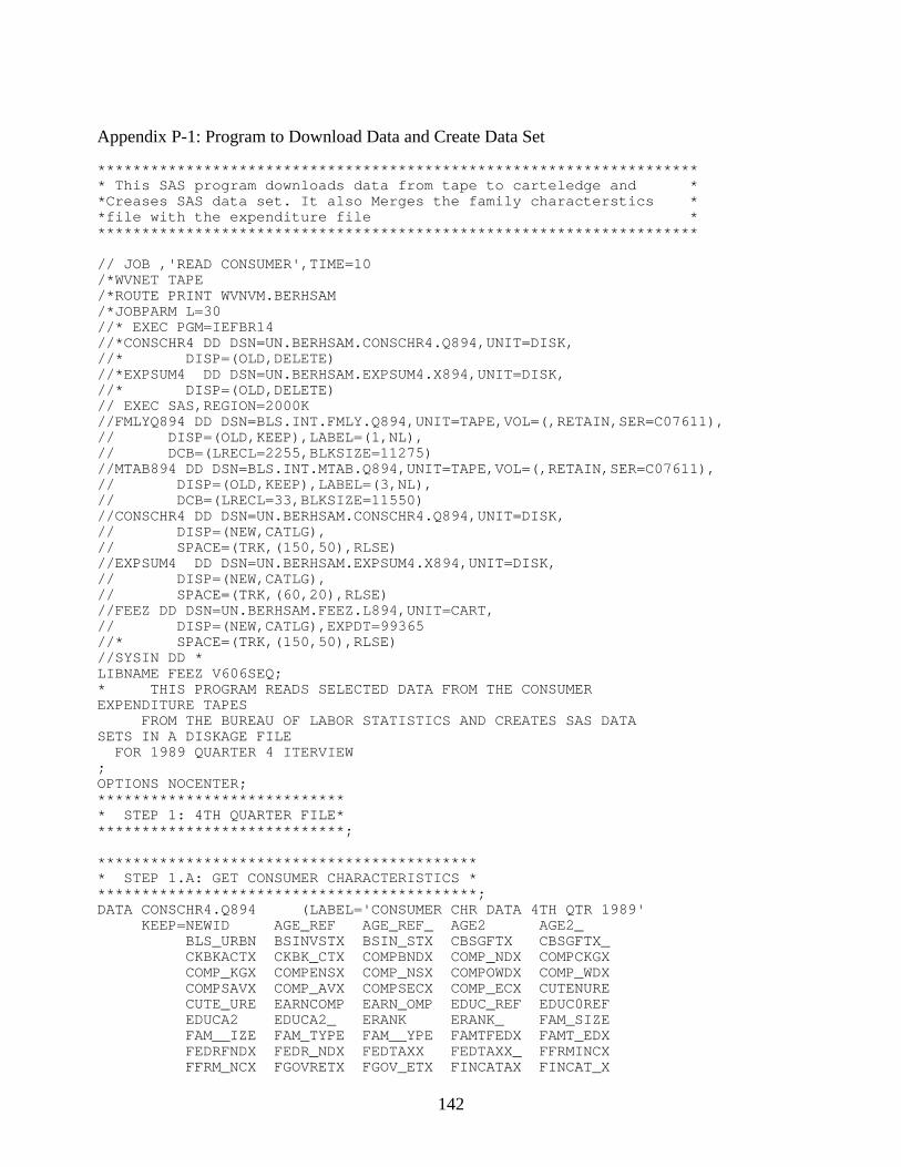
142

Appendix P-1: Program to Download Data and Create Data Set

********************************************************************* This SAS program downloads data from tape to carteledge and **Creases SAS data set. It also Merges the family characterstics **file with the expenditure file *********************************************************************

// JOB ,'READ CONSUMER',TIME=10/*WVNET TAPE/*ROUTE PRINT WVNVM.BERHSAM/*JOBPARM L=30//* EXEC PGM=IEFBR14//*CONSCHR4 DD DSN=UN.BERHSAM.CONSCHR4.Q894,UNIT=DISK,//* DISP=(OLD,DELETE)//*EXPSUM4 DD DSN=UN.BERHSAM.EXPSUM4.X894,UNIT=DISK,//* DISP=(OLD,DELETE)// EXEC SAS,REGION=2000K//FMLYQ894 DD DSN=BLS.INT.FMLY.Q894,UNIT=TAPE,VOL=(,RETAIN,SER=C07611),// DISP=(OLD,KEEP),LABEL=(1,NL),// DCB=(LRECL=2255,BLKSIZE=11275)//MTAB894 DD DSN=BLS.INT.MTAB.Q894,UNIT=TAPE,VOL=(,RETAIN,SER=C07611),// DISP=(OLD,KEEP),LABEL=(3,NL),// DCB=(LRECL=33,BLKSIZE=11550)//CONSCHR4 DD DSN=UN.BERHSAM.CONSCHR4.Q894,UNIT=DISK,// DISP=(NEW,CATLG),// SPACE=(TRK,(150,50),RLSE)//EXPSUM4 DD DSN=UN.BERHSAM.EXPSUM4.X894,UNIT=DISK,// DISP=(NEW,CATLG),// SPACE=(TRK,(60,20),RLSE)//FEEZ DD DSN=UN.BERHSAM.FEEZ.L894,UNIT=CART,// DISP=(NEW,CATLG),EXPDT=99365//* SPACE=(TRK,(150,50),RLSE)//SYSIN DD *LIBNAME FEEZ V606SEQ;* THIS PROGRAM READS SELECTED DATA FROM THE CONSUMEREXPENDITURE TAPES FROM THE BUREAU OF LABOR STATISTICS AND CREATES SAS DATASETS IN A DISKAGE FILE FOR 1989 QUARTER 4 ITERVIEW;OPTIONS NOCENTER;***************************** STEP 1: 4TH QUARTER FILE*****************************; ******************************************** STEP 1.A: GET CONSUMER CHARACTERISTICS ********************************************;DATA CONSCHR4.Q894 (LABEL='CONSUMER CHR DATA 4TH QTR 1989' KEEP=NEWID AGE_REF AGE_REF_ AGE2 AGE2_ BLS_URBN BSINVSTX BSIN_STX CBSGFTX CBSGFTX_ CKBKACTX CKBK_CTX COMPBNDX COMP_NDX COMPCKGX COMP_KGX COMPENSX COMP_NSX COMPOWDX COMP_WDX COMPSAVX COMP_AVX COMPSECX COMP_ECX CUTENURE CUTE_URE EARNCOMP EARN_OMP EDUC_REF EDUC0REF EDUCA2 EDUCA2_ ERANK ERANK_ FAM_SIZE FAM__IZE FAM_TYPE FAM__YPE FAMTFEDX FAMT_EDX FEDRFNDX FEDR_NDX FEDTAXX FEDTAXX_ FFRMINCX FFRM_NCX FGOVRETX FGOV_ETX FINCATAX FINCAT_X

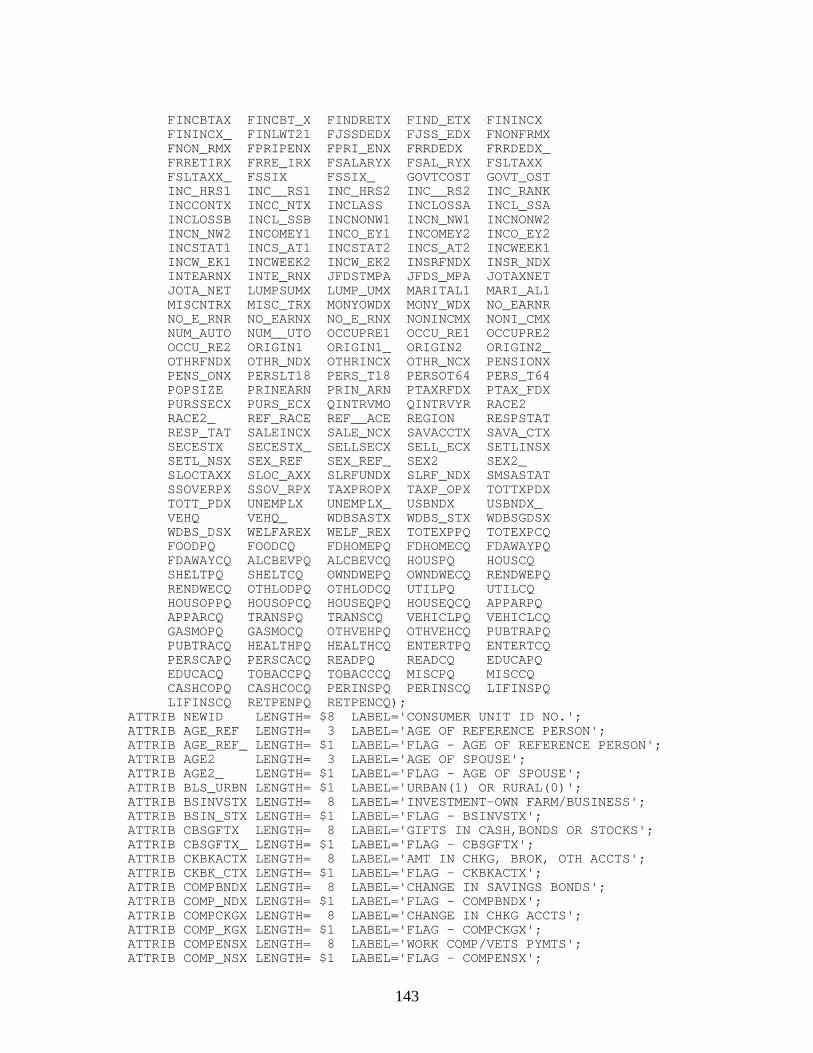
143

FINCBTAX FINCBT_X FINDRETX FIND_ETX FININCX FININCX_ FINLWT21 FJSSDEDX FJSS_EDX FNONFRMX FNON_RMX FPRIPENX FPRI_ENX FRRDEDX FRRDEDX_ FRRETIRX FRRE_IRX FSALARYX FSAL_RYX FSLTAXX FSLTAXX_ FSSIX FSSIX_ GOVTCOST GOVT_OST INC_HRS1 INC__RS1 INC_HRS2 INC__RS2 INC_RANK INCCONTX INCC_NTX INCLASS INCLOSSA INCL_SSA INCLOSSB INCL_SSB INCNONW1 INCN_NW1 INCNONW2 INCN_NW2 INCOMEY1 INCO_EY1 INCOMEY2 INCO_EY2 INCSTAT1 INCS_AT1 INCSTAT2 INCS_AT2 INCWEEK1 INCW_EK1 INCWEEK2 INCW_EK2 INSRFNDX INSR_NDX INTEARNX INTE_RNX JFDSTMPA JFDS_MPA JOTAXNET JOTA_NET LUMPSUMX LUMP_UMX MARITAL1 MARI_AL1 MISCNTRX MISC_TRX MONYOWDX MONY_WDX NO_EARNR NO_E_RNR NO_EARNX NO_E_RNX NONINCMX NONI_CMX NUM_AUTO NUM__UTO OCCUPRE1 OCCU_RE1 OCCUPRE2 OCCU_RE2 ORIGIN1 ORIGIN1_ ORIGIN2 ORIGIN2_ OTHRFNDX OTHR_NDX OTHRINCX OTHR_NCX PENSIONX PENS_ONX PERSLT18 PERS_T18 PERSOT64 PERS_T64 POPSIZE PRINEARN PRIN_ARN PTAXRFDX PTAX_FDX PURSSECX PURS_ECX QINTRVMO QINTRVYR RACE2 RACE2_ REF_RACE REF__ACE REGION RESPSTAT RESP_TAT SALEINCX SALE_NCX SAVACCTX SAVA_CTX SECESTX SECESTX_ SELLSECX SELL_ECX SETLINSX SETL_NSX SEX_REF SEX_REF_ SEX2 SEX2_ SLOCTAXX SLOC_AXX SLRFUNDX SLRF_NDX SMSASTAT SSOVERPX SSOV_RPX TAXPROPX TAXP_OPX TOTTXPDX TOTT_PDX UNEMPLX UNEMPLX_ USBNDX USBNDX_ VEHQ VEHQ_ WDBSASTX WDBS_STX WDBSGDSX WDBS_DSX WELFAREX WELF_REX TOTEXPPQ TOTEXPCQ FOODPQ FOODCQ FDHOMEPQ FDHOMECQ FDAWAYPQ FDAWAYCQ ALCBEVPQ ALCBEVCQ HOUSPQ HOUSCQ SHELTPQ SHELTCQ OWNDWEPQ OWNDWECQ RENDWEPQ RENDWECQ OTHLODPQ OTHLODCQ UTILPQ UTILCQ HOUSOPPQ HOUSOPCQ HOUSEQPQ HOUSEQCQ APPARPQ APPARCQ TRANSPQ TRANSCQ VEHICLPQ VEHICLCQ GASMOPQ GASMOCQ OTHVEHPQ OTHVEHCQ PUBTRAPQ PUBTRACQ HEALTHPQ HEALTHCQ ENTERTPQ ENTERTCQ PERSCAPQ PERSCACQ READPQ READCQ EDUCAPQ EDUCACQ TOBACCPQ TOBACCCQ MISCPQ MISCCQ CASHCOPQ CASHCOCQ PERINSPQ PERINSCQ LIFINSPQ LIFINSCQ RETPENPQ RETPENCQ); ATTRIB NEWID LENGTH= $8 LABEL='CONSUMER UNIT ID NO.'; ATTRIB AGE_REF LENGTH= 3 LABEL='AGE OF REFERENCE PERSON'; ATTRIB AGE_REF_ LENGTH= $1 LABEL='FLAG - AGE OF REFERENCE PERSON'; ATTRIB AGE2 LENGTH= 3 LABEL='AGE OF SPOUSE'; ATTRIB AGE2_ LENGTH= $1 LABEL='FLAG - AGE OF SPOUSE'; ATTRIB BLS_URBN LENGTH= $1 LABEL='URBAN(1) OR RURAL(0)'; ATTRIB BSINVSTX LENGTH= 8 LABEL='INVESTMENT-OWN FARM/BUSINESS'; ATTRIB BSIN_STX LENGTH= $1 LABEL='FLAG - BSINVSTX'; ATTRIB CBSGFTX LENGTH= 8 LABEL='GIFTS IN CASH,BONDS OR STOCKS'; ATTRIB CBSGFTX_ LENGTH= $1 LABEL='FLAG - CBSGFTX'; ATTRIB CKBKACTX LENGTH= 8 LABEL='AMT IN CHKG, BROK, OTH ACCTS'; ATTRIB CKBK_CTX LENGTH= $1 LABEL='FLAG - CKBKACTX'; ATTRIB COMPBNDX LENGTH= 8 LABEL='CHANGE IN SAVINGS BONDS'; ATTRIB COMP_NDX LENGTH= $1 LABEL='FLAG - COMPBNDX'; ATTRIB COMPCKGX LENGTH= 8 LABEL='CHANGE IN CHKG ACCTS'; ATTRIB COMP_KGX LENGTH= $1 LABEL='FLAG - COMPCKGX'; ATTRIB COMPENSX LENGTH= 8 LABEL='WORK COMP/VETS PYMTS'; ATTRIB COMP_NSX LENGTH= $1 LABEL='FLAG - COMPENSX';

144

ATTRIB COMPOWDX LENGTH= 8 LABEL='CHANGE IN MONEY OWED CU'; ATTRIB COMP_WDX LENGTH= $1 LABEL='FLAG - COMPOWDX'; ATTRIB COMPSAVX LENGTH= 8 LABEL='CHANGE IN SVGS ACCT'; ATTRIB COMP_AVX LENGTH= $1 LABEL='FLAG - COMPSAVX'; ATTRIB COMPSECX LENGTH= 8 LABEL='CHANGE IN STKS, BNDS'; ATTRIB COMP_ECX LENGTH= $1 LABEL='FLAG - COMPSECX'; ATTRIB CUTENURE LENGTH= $1 LABEL='HOUSING TENURE: 1-6'; ATTRIB CUTE_URE LENGTH= $1 LABEL='FLAG - CUTENURE'; ATTRIB EARNCOMP LENGTH= $1 LABEL='COMPOSITION OF EARNERS 1-8'; ATTRIB EARN_OMP LENGTH= $1 LABEL='FLAG - EARNCOMP'; ATTRIB EDUC_REF LENGTH= $1 LABEL='EDUCATION OF REF. PERSON 1-7'; ATTRIB EDUC0REF LENGTH= $1 LABEL='FLAG - EDUC_REF'; ATTRIB EDUCA2 LENGTH= $1 LABEL='EDUCATION OF SPOUSE 0-32'; ATTRIB EDUCA2_ LENGTH= $1 LABEL='FLAG - EDUCA2'; ATTRIB ERANK LENGTH= 8 LABEL='WTD. RANKING BY EXPENDS. (9.7)'; ATTRIB ERANK_ LENGTH= $1 LABEL='FLAG - ERANK'; ATTRIB FAM_SIZE LENGTH= 2 LABEL='NO. OF MEMBRS IN CONS. UNIT'; ATTRIB FAM__IZE LENGTH= $1 LABEL='FLAG - FAM_SIZE'; ATTRIB FAM_TYPE LENGTH= $1 LABEL='CONS. UNIT TYPE 1-9'; ATTRIB FAM__YPE LENGTH= $1 LABEL='FLAG - FAM_TYPE'; ATTRIB FAMTFEDX LENGTH= 8 LABEL='FED Y TX WHLD LAST CHK-ANNUAL.'; ATTRIB FAMT_EDX LENGTH= $1 LABEL='FLAG - FAMTFEDX'; ATTRIB FEDRFNDX LENGTH= 8 LABEL='REFUND FROM FED INCOME TAX'; ATTRIB FEDR_NDX LENGTH= $1 LABEL='FLAG - FEDRFNDX'; ATTRIB FEDTAXX LENGTH= 8 LABEL='FEDERAL TAX PAID'; ATTRIB FEDTAXX_ LENGTH= $1 LABEL='FLAG - FEDTAXX'; ATTRIB FFRMINCX LENGTH= 8 LABEL='INCOME/LOSS FROM OWN FARM'; ATTRIB FFRM_NCX LENGTH= $1 LABEL='FLAG - FFRMINCX'; ATTRIB FGOVRETX LENGTH= 8 LABEL='GOVT RETIREMT DEDUCTED'; ATTRIB FGOV_ETX LENGTH= $1 LABEL='FLAG - FGOVRETX'; ATTRIB FINCATAX LENGTH= 8 LABEL='CONS. UNIT INCOME AFTER TAXES'; ATTRIB FINCAT_X LENGTH= $1 LABEL='FLAG - FINCATAX'; ATTRIB FINCBTAX LENGTH= 8 LABEL='CONS. UNIT INCOME BEFORE TAXES'; ATTRIB FINCBT_X LENGTH= $1 LABEL='FLAG - FINCBTAX'; ATTRIB FINDRETX LENGTH= 8 LABEL='SELF-EMPLOYED RETIREMENT PLAN'; ATTRIB FIND_ETX LENGTH= $1 LABEL='FLAG - FINCRETX'; ATTRIB FININCX LENGTH= 8 LABEL='DIVID/ROYALTIES/ESTATES/TRUSTS'; ATTRIB FININCX_ LENGTH= $1 LABEL='FLAG - FININCX'; ATTRIB FINLWT21 LENGTH= 8 LABEL='CONS. UNIT WEIGHT (11.3)'; ATTRIB FJSSDEDX LENGTH= 8 LABEL='SOC SEC PAYMENT'; ATTRIB FJSS_EDX LENGTH= $1 LABEL='FLAG - FJSSDEDX'; ATTRIB FNONFRMX LENGTH= 8 LABEL='INC. FROM NONFARM BUSINESS'; ATTRIB FNON_RMX LENGTH= $1 LABEL='FLAG - FNON_RMX'; ATTRIB FPRIPENX LENGTH= 8 LABEL='PRIV. PENS. DEDUCT. FR LAST PAY'; ATTRIB FPRI_ENX LENGTH= $1 LABEL='FLAG - FRIPENX'; ATTRIB FRRDEDX LENGTH= 8 LABEL='RAIL. RETIR. DEDUCT FR LAST PAY'; ATTRIB FRRDEDX_ LENGTH= $1 LABEL='FLAG - FRRDEDX'; ATTRIB FRRETIRX LENGTH= 8 LABEL='AMT. FROM RRR AND SS'; ATTRIB FRRE_IRX LENGTH= $1 LABEL='FLAG - FRRETIRX'; ATTRIB FSALARYX LENGTH= 8 LABEL='WAGE AND SALARY INCOME'; ATTRIB FSAL_RYX LENGTH= $1 LABEL='FLAG - FSALARYX'; ATTRIB FSLTAXX LENGTH= 8 LABEL='ST. AND LOCAL INCOME TAXES'; ATTRIB FSLTAXX_ LENGTH= $1 LABEL='FLAG - FSLTAXX'; ATTRIB FSSIX LENGTH= 8 LABEL='COMBINES SSI CHECKS'; ATTRIB FSSIX_ LENGTH= $1 LABEL='FLAG - FSSIX'; ATTRIB GOVTCOST LENGTH= $1 LABEL='GOVT. PAYS HOUSING 1-2'; ATTRIB GOVT_OST LENGTH= $1 LABEL='FLAG - GOVTCOST'; ATTRIB INC_HRS1 LENGTH= 3 LABEL='HOURS WORKED/WK BY REF. PERSON'; ATTRIB INC__RS1 LENGTH= $1 LABEL='FLAG - INC_HRS1'; ATTRIB INC_HRS2 LENGTH= 3 LABEL='HOURS WORKED/WEEK BY SPOUSE';

145

ATTRIB INC__RS2 LENGTH= $1 LABEL='FLAG - INC_HRS2'; ATTRIB INC_RANK LENGTH= 8 LABEL='WEIGHTED % INCOME RANKING(9.7)'; ATTRIB INCCONTX LENGTH= 8 LABEL='REGULAR CONTRIB. RECEIVED'; ATTRIB INCC_NTX LENGTH= $1 LABEL='FLAG - INCCONTX'; ATTRIB INCLASS LENGTH= $1 LABEL='INCOME CLASS 1-8'; ATTRIB INCLOSSA LENGTH= 8 LABEL='LOSS FROM RENTERS'; ATTRIB INCL_SSA LENGTH= $1 LABEL='FLAG - INCLOSSA'; ATTRIB INCLOSSB LENGTH= 8 LABEL='LOSS FROM OTHER RENTAL UNITS'; ATTRIB INCL_SSB LENGTH= $1 LABEL='FLAG - INCLOSSB'; ATTRIB INCNONW1 LENGTH= $1 LABEL='REAS. REF PER NOT WORKING 1-6'; ATTRIB INCN_NW1 LENGTH= $1 LABEL='FLAG - INCNONW1'; ATTRIB INCNONW2 LENGTH= $1 LABEL='REAS. SPOUSE NOT WORKING 1-6'; ATTRIB INCN_NW2 LENGTH= $1 LABEL='FLAG - INCNONW2'; ATTRIB INCOMEY1 LENGTH= $1 LABEL='PREV TYPE EMPLOYEE-REF PERS 1-6'; ATTRIB INCO_EY1 LENGTH= $1 LABEL='FLAG - INCOMEY1'; ATTRIB INCOMEY2 LENGTH= $1 LABEL='PREV TYPE EMPLOYEE-SPOUSE 1-6'; ATTRIB INCO_EY2 LENGTH= $1 LABEL='FLAG - INCOMEY2'; ATTRIB INCSTAT1 LENGTH= $1 LABEL='WORK STATUS-REF PERS 1-2'; ATTRIB INCS_AT1 LENGTH= $1 LABEL='FLAG - INCSTAT1'; ATTRIB INCSTAT2 LENGTH= $1 LABEL='WORK STATUS-SPOUSE 1-2'; ATTRIB INCS_AT2 LENGTH= $1 LABEL='FLAG - INCSTAT2'; ATTRIB INCWEEK1 LENGTH= 2 LABEL='WEEKS WORKED-REF PERS'; ATTRIB INCW_EK1 LENGTH= $1 LABEL='FLAG - INCWEEK1'; ATTRIB INCWEEK2 LENGTH= 2 LABEL='WEEKS WORKED-SPOUSE'; ATTRIB INCW_EK2 LENGTH= $1 LABEL='FLAG - INCWEEK2'; ATTRIB INSRFNDX LENGTH= 8 LABEL='REFUND FROM INSURANCE POL.'; ATTRIB INSR_NDX LENGTH= $1 LABEL='FLAG - INSRFNDX'; ATTRIB INTEARNX LENGTH= 8 LABEL='INTEREST-SVGS ACCTS OR BONDS'; ATTRIB INTE_RNX LENGTH= $1 LABEL='FLAG - INTEARNX'; ATTRIB JFDSTMPA LENGTH= 8 LABEL='ANNUAL VALUE OF FOOD STAMPS'; ATTRIB JFDS_MPA LENGTH= $1 LABEL='FLAG - JFDSTMPA'; ATTRIB JOTAXNET LENGTH= 8 LABEL='OTH TAXES PD DURING PAST YR'; ATTRIB JOTA_NET LENGTH= $1 LABEL='FLAG - JOTAXNET'; ATTRIB LUMPSUMX LENGTH= 8 LABEL='LUMP SUM RECEIPTS'; ATTRIB LUMP_UMX LENGTH= $1 LABEL='FLAG - LUMPSUMX'; ATTRIB MARITAL1 LENGTH= $1 LABEL='MARITAL STATUS OF REF PER 1-5'; ATTRIB MARI_AL1 LENGTH= $1 LABEL='FLAG - MARITAL1'; ATTRIB MISCNTRX LENGTH= 8 LABEL='CONTRIBS. TO OTH. ORGS.'; ATTRIB MISC_TRX LENGTH= $1 LABEL='FLAG - MISCNTRX'; ATTRIB MONYOWDX LENGTH= 8 LABEL='MONEY OWED TO CU'; ATTRIB MONY_WDX LENGTH= $1 LABEL='FLAG - MONYOWDX'; ATTRIB NO_EARNR LENGTH= 2 LABEL='NO. EARNERS'; ATTRIB NO_E_RNR LENGTH= $1 LABEL='FLAG - NO_EARNR'; ATTRIB NO_EARNX LENGTH= 8 LABEL='INCOME OTHER THAN EARNINGS'; ATTRIB NO_E_RNX LENGTH= $1 LABEL='FLAG - NO_EARNX'; ATTRIB NONINCMX LENGTH= 8 LABEL='OTH. MONEY EXCL FR FINCBEFTX'; ATTRIB NONI_CMX LENGTH= $1 LABEL='FLAG - NONINCMX'; ATTRIB NUM_AUTO LENGTH= 2 LABEL='NO. OR AUTOS'; ATTRIB NUM__UTO LENGTH= $1 LABEL='FLAG - NUMAUTO'; ATTRIB OCCUPRE1 LENGTH= $2 LABEL='REF PER OCCUPATION 01-11'; ATTRIB OCCU_RE1 LENGTH= $1 LABEL='FLAG - OCCUPRE1'; ATTRIB OCCUPRE2 LENGTH= $2 LABEL='SPOUSES OCCUPATION 01-11'; ATTRIB OCCU_RE2 LENGTH= $1 LABEL='FLAG - OCCUPRE2'; ATTRIB ORIGIN1 LENGTH= $1 LABEL='ORIGIN OF REF. PERSON (1-4)'; ATTRIB ORIGIN1_ LENGTH= $1 LABEL='FLAG - ORIGIN1'; ATTRIB ORIGIN2 LENGTH= $1 LABEL='ORIGIN OF SPOUSE (1-4)'; ATTRIB ORIGIN2_ LENGTH= $1 LABEL='FLAG - ORIGIN2'; ATTRIB OTHRFNDX LENGTH= 8 LABEL='REFUND FROM OTHER SOURCES'; ATTRIB OTHR_NDX LENGTH= $1 LABEL='FLAG - OTHRFNDX'; ATTRIB OTHRINCX LENGTH= 8 LABEL='OTHER MONEY INCOME';

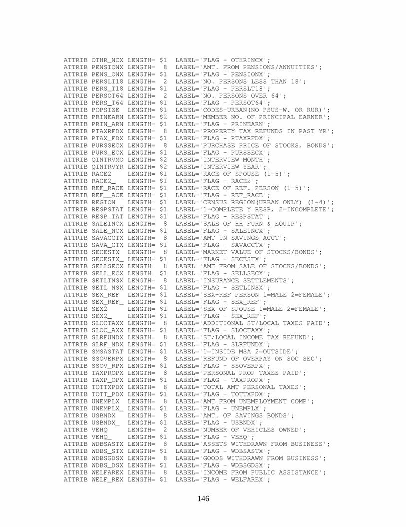
146

ATTRIB OTHR_NCX LENGTH= $1 LABEL='FLAG - OTHRINCX'; ATTRIB PENSIONX LENGTH= 8 LABEL='AMT. FROM PENSIONS/ANNUITIES'; ATTRIB PENS_ONX LENGTH= $1 LABEL='FLAG - PENSIONX'; ATTRIB PERSLT18 LENGTH= 2 LABEL='NO. PERSONS LESS THAN 18'; ATTRIB PERS_T18 LENGTH= $1 LABEL='FLAG - PERSLT18'; ATTRIB PERSOT64 LENGTH= 2 LABEL='NO. PERSONS OVER 64'; ATTRIB PERS_T64 LENGTH= $1 LABEL='FLAG - PERSOT64'; ATTRIB POPSIZE LENGTH= $1 LABEL='CODES-URBAN(NO PSUS-W. OR RUR)'; ATTRIB PRINEARN LENGTH= $2 LABEL='MEMBER NO. OF PRINCIPAL EARNER'; ATTRIB PRIN_ARN LENGTH= $1 LABEL='FLAG - PRINEARN'; ATTRIB PTAXRFDX LENGTH= 8 LABEL='PROPERTY TAX REFUNDS IN PAST YR'; ATTRIB PTAX_FDX LENGTH= $1 LABEL='FLAG - PTAXRFDX'; ATTRIB PURSSECX LENGTH= 8 LABEL='PURCHASE PRICE OF STOCKS, BONDS'; ATTRIB PURS_ECX LENGTH= $1 LABEL='FLAG - PURSSECX'; ATTRIB QINTRVMO LENGTH= $2 LABEL='INTERVIEW MONTH'; ATTRIB QINTRVYR LENGTH= $2 LABEL='INTERVIEW YEAR'; ATTRIB RACE2 LENGTH= $1 LABEL='RACE OF SPOUSE (1-5)'; ATTRIB RACE2_ LENGTH= $1 LABEL='FLAG - RACE2'; ATTRIB REF_RACE LENGTH= $1 LABEL='RACE OF REF. PERSON (1-5)'; ATTRIB REF__ACE LENGTH= $1 LABEL='FLAG - REF_RACE'; ATTRIB REGION LENGTH= $1 LABEL='CENSUS REGION(URBAN ONLY) (1-4)'; ATTRIB RESPSTAT LENGTH= $1 LABEL='1=COMPLETE Y RESP, 2=INCOMPLETE'; ATTRIB RESP_TAT LENGTH= $1 LABEL='FLAG - RESPSTAT'; ATTRIB SALEINCX LENGTH= 8 LABEL='SALE OF HH FURN & EQUIP'; ATTRIB SALE_NCX LENGTH= $1 LABEL='FLAG - SALEINCX'; ATTRIB SAVACCTX LENGTH= 8 LABEL='AMT IN SAVINGS ACCT'; ATTRIB SAVA_CTX LENGTH= $1 LABEL='FLAG - SAVACCTX'; ATTRIB SECESTX LENGTH= 8 LABEL='MARKET VALUE OF STOCKS/BONDS'; ATTRIB SECESTX_ LENGTH= $1 LABEL='FLAG - SECESTX'; ATTRIB SELLSECX LENGTH= 8 LABEL='AMT FROM SALE OF STOCKS/BONDS'; ATTRIB SELL_ECX LENGTH= $1 LABEL='FLAG - SELLSECX'; ATTRIB SETLINSX LENGTH= 8 LABEL='INSURANCE SETTLEMENTS'; ATTRIB SETL_NSX LENGTH= $1 LABEL='FLAG - SETLINSX'; ATTRIB SEX_REF LENGTH= $1 LABEL='SEX-REF PERSON 1=MALE 2=FEMALE'; ATTRIB SEX_REF_ LENGTH= $1 LABEL='FLAG - SEX_REF'; ATTRIB SEX2 LENGTH= $1 LABEL='SEX OF SPOUSE 1=MALE 2=FEMALE'; ATTRIB SEX2_ LENGTH= $1 LABEL='FLAG - SEX_REF'; ATTRIB SLOCTAXX LENGTH= 8 LABEL='ADDITIONAL ST/LOCAL TAXES PAID'; ATTRIB SLOC_AXX LENGTH= $1 LABEL='FLAG - SLOCTAXX'; ATTRIB SLRFUNDX LENGTH= 8 LABEL='ST/LOCAL INCOME TAX REFUND'; ATTRIB SLRF_NDX LENGTH= $1 LABEL='FLAG - SLRFUNDX'; ATTRIB SMSASTAT LENGTH= $1 LABEL='1=INSIDE MSA 2=OUTSIDE'; ATTRIB SSOVERPX LENGTH= 8 LABEL='REFUND OF OVERPAY ON SOC SEC'; ATTRIB SSOV_RPX LENGTH= $1 LABEL='FLAG - SSOVERPX'; ATTRIB TAXPROPX LENGTH= 8 LABEL='PERSONAL PROP TAXES PAID'; ATTRIB TAXP_OPX LENGTH= $1 LABEL='FLAG - TAXPROPX'; ATTRIB TOTTXPDX LENGTH= 8 LABEL='TOTAL AMT PERSONAL TAXES'; ATTRIB TOTT_PDX LENGTH= $1 LABEL='FLAG - TOTTXPDX'; ATTRIB UNEMPLX LENGTH= 8 LABEL='AMT FROM UNEMPLOYMENT COMP'; ATTRIB UNEMPLX_ LENGTH= $1 LABEL='FLAG - UNEMPLX'; ATTRIB USBNDX LENGTH= 8 LABEL='AMT. OF SAVINGS BONDS'; ATTRIB USBNDX_ LENGTH= $1 LABEL='FLAG - USBNDX'; ATTRIB VEHQ LENGTH= 2 LABEL='NUMBER OF VEHICLES OWNED'; ATTRIB VEHQ_ LENGTH= $1 LABEL='FLAG - VEHQ'; ATTRIB WDBSASTX LENGTH= 8 LABEL='ASSETS WITHDRAWN FROM BUSINESS'; ATTRIB WDBS_STX LENGTH= $1 LABEL='FLAG - WDBSASTX'; ATTRIB WDBSGDSX LENGTH= 8 LABEL='GOODS WITHDRAWN FROM BUSINESS'; ATTRIB WDBS_DSX LENGTH= $1 LABEL='FLAG - WDBSGDSX'; ATTRIB WELFAREX LENGTH= 8 LABEL='INCOME FROM PUBLIC ASSISTANCE'; ATTRIB WELF_REX LENGTH= $1 LABEL='FLAG - WELFAREX';

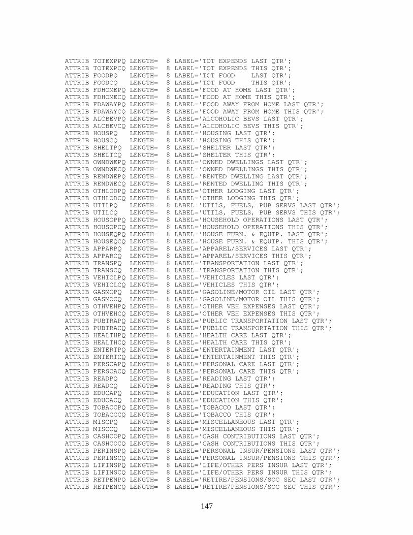
147

ATTRIB TOTEXPPQ LENGTH= 8 LABEL='TOT EXPENDS LAST QTR'; ATTRIB TOTEXPCQ LENGTH= 8 LABEL='TOT EXPENDS THIS QTR'; ATTRIB FOODPQ LENGTH= 8 LABEL='TOT FOOD LAST QTR'; ATTRIB FOODCQ LENGTH= 8 LABEL='TOT FOOD THIS QTR'; ATTRIB FDHOMEPQ LENGTH= 8 LABEL='FOOD AT HOME LAST QTR'; ATTRIB FDHOMECQ LENGTH= 8 LABEL='FOOD AT HOME THIS QTR'; ATTRIB FDAWAYPQ LENGTH= 8 LABEL='FOOD AWAY FROM HOME LAST QTR'; ATTRIB FDAWAYCQ LENGTH= 8 LABEL='FOOD AWAY FROM HOME THIS QTR'; ATTRIB ALCBEVPQ LENGTH= 8 LABEL='ALCOHOLIC BEVS LAST QTR'; ATTRIB ALCBEVCQ LENGTH= 8 LABEL='ALCOHOLIC BEVS THIS QTR'; ATTRIB HOUSPQ LENGTH= 8 LABEL='HOUSING LAST QTR'; ATTRIB HOUSCQ LENGTH= 8 LABEL='HOUSING THIS QTR'; ATTRIB SHELTPQ LENGTH= 8 LABEL='SHELTER LAST QTR'; ATTRIB SHELTCQ LENGTH= 8 LABEL='SHELTER THIS QTR'; ATTRIB OWNDWEPQ LENGTH= 8 LABEL='OWNED DWELLINGS LAST QTR'; ATTRIB OWNDWECQ LENGTH= 8 LABEL='OWNED DWELLINGS THIS QTR'; ATTRIB RENDWEPQ LENGTH= 8 LABEL='RENTED DWELLING LAST QTR'; ATTRIB RENDWECQ LENGTH= 8 LABEL='RENTED DWELLING THIS QTR'; ATTRIB OTHLODPQ LENGTH= 8 LABEL='OTHER LODGING LAST QTR'; ATTRIB OTHLODCQ LENGTH= 8 LABEL='OTHER LODGING THIS QTR'; ATTRIB UTILPQ LENGTH= 8 LABEL='UTILS, FUELS, PUB SERVS LAST QTR'; ATTRIB UTILCQ LENGTH= 8 LABEL='UTILS, FUELS, PUB SERVS THIS QTR'; ATTRIB HOUSOPPQ LENGTH= 8 LABEL='HOUSEHOLD OPERATIONS LAST QTR'; ATTRIB HOUSOPCQ LENGTH= 8 LABEL='HOUSEHOLD OPERATIONS THIS QTR'; ATTRIB HOUSEQPQ LENGTH= 8 LABEL='HOUSE FURN. & EQUIP. LAST QTR'; ATTRIB HOUSEQCQ LENGTH= 8 LABEL='HOUSE FURN. & EQUIP. THIS QTR'; ATTRIB APPARPQ LENGTH= 8 LABEL='APPAREL/SERVICES LAST QTR'; ATTRIB APPARCQ LENGTH= 8 LABEL='APPAREL/SERVICES THIS QTR'; ATTRIB TRANSPQ LENGTH= 8 LABEL='TRANSPORTATION LAST QTR'; ATTRIB TRANSCQ LENGTH= 8 LABEL='TRANSPORTATION THIS QTR'; ATTRIB VEHICLPQ LENGTH= 8 LABEL='VEHICLES LAST QTR'; ATTRIB VEHICLCQ LENGTH= 8 LABEL='VEHICLES THIS QTR'; ATTRIB GASMOPQ LENGTH= 8 LABEL='GASOLINE/MOTOR OIL LAST QTR'; ATTRIB GASMOCQ LENGTH= 8 LABEL='GASOLINE/MOTOR OIL THIS QTR'; ATTRIB OTHVEHPQ LENGTH= 8 LABEL='OTHER VEH EXPENSES LAST QTR'; ATTRIB OTHVEHCQ LENGTH= 8 LABEL='OTHER VEH EXPENSES THIS QTR'; ATTRIB PUBTRAPQ LENGTH= 8 LABEL='PUBLIC TRANSPORTATION LAST QTR'; ATTRIB PUBTRACQ LENGTH= 8 LABEL='PUBLIC TRANSPORTATION THIS QTR'; ATTRIB HEALTHPQ LENGTH= 8 LABEL='HEALTH CARE LAST QTR'; ATTRIB HEALTHCQ LENGTH= 8 LABEL='HEALTH CARE THIS QTR'; ATTRIB ENTERTPQ LENGTH= 8 LABEL='ENTERTAINMENT LAST QTR'; ATTRIB ENTERTCQ LENGTH= 8 LABEL='ENTERTAINMENT THIS QTR'; ATTRIB PERSCAPQ LENGTH= 8 LABEL='PERSONAL CARE LAST QTR'; ATTRIB PERSCACQ LENGTH= 8 LABEL='PERSONAL CARE THIS QTR'; ATTRIB READPQ LENGTH= 8 LABEL='READING LAST QTR'; ATTRIB READCQ LENGTH= 8 LABEL='READING THIS QTR'; ATTRIB EDUCAPQ LENGTH= 8 LABEL='EDUCATION LAST QTR'; ATTRIB EDUCACQ LENGTH= 8 LABEL='EDUCATION THIS QTR'; ATTRIB TOBACCPQ LENGTH= 8 LABEL='TOBACCO LAST QTR'; ATTRIB TOBACCCQ LENGTH= 8 LABEL='TOBACCO THIS QTR'; ATTRIB MISCPQ LENGTH= 8 LABEL='MISCELLANEOUS LAST QTR'; ATTRIB MISCCQ LENGTH= 8 LABEL='MISCELLANEOUS THIS QTR'; ATTRIB CASHCOPQ LENGTH= 8 LABEL='CASH CONTRIBUTIONS LAST QTR'; ATTRIB CASHCOCQ LENGTH= 8 LABEL='CASH CONTRIBUTIONS THIS QTR'; ATTRIB PERINSPQ LENGTH= 8 LABEL='PERSONAL INSUR/PENSIONS LAST QTR'; ATTRIB PERINSCQ LENGTH= 8 LABEL='PERSONAL INSUR/PENSIONS THIS QTR'; ATTRIB LIFINSPQ LENGTH= 8 LABEL='LIFE/OTHER PERS INSUR LAST QTR'; ATTRIB LIFINSCQ LENGTH= 8 LABEL='LIFE/OTHER PERS INSUR THIS QTR'; ATTRIB RETPENPQ LENGTH= 8 LABEL='RETIRE/PENSIONS/SOC SEC LAST QTR'; ATTRIB RETPENCQ LENGTH= 8 LABEL='RETIRE/PENSIONS/SOC SEC THIS QTR';

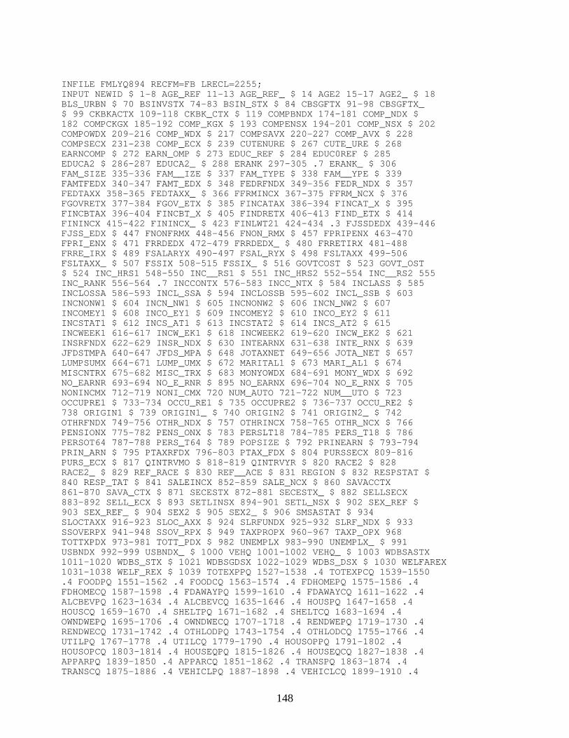
148

INFILE FMLYQ894 RECFM=FB LRECL=2255;INPUT NEWID $ 1-8 AGE_REF 11-13 AGE_REF_ $ 14 AGE2 15-17 AGE2_ $ 18BLS_URBN $ 70 BSINVSTX 74-83 BSIN_STX $ 84 CBSGFTX 91-98 CBSGFTX_$ 99 CKBKACTX 109-118 CKBK_CTX $ 119 COMPBNDX 174-181 COMP_NDX $182 COMPCKGX 185-192 COMP_KGX $ 193 COMPENSX 194-201 COMP_NSX $ 202COMPOWDX 209-216 COMP_WDX $ 217 COMPSAVX 220-227 COMP_AVX $ 228COMPSECX 231-238 COMP_ECX $ 239 CUTENURE $ 267 CUTE_URE $ 268EARNCOMP $ 272 EARN_OMP $ 273 EDUC_REF $ 284 EDUC0REF $ 285EDUCA2 $ 286-287 EDUCA2_ $ 288 ERANK 297-305 .7 ERANK_ $ 306FAM_SIZE 335-336 FAM__IZE $ 337 FAM_TYPE $ 338 FAM__YPE $ 339FAMTFEDX 340-347 FAMT_EDX $ 348 FEDRFNDX 349-356 FEDR_NDX $ 357FEDTAXX 358-365 FEDTAXX_ $ 366 FFRMINCX 367-375 FFRM_NCX $ 376FGOVRETX 377-384 FGOV_ETX $ 385 FINCATAX 386-394 FINCAT_X $ 395FINCBTAX 396-404 FINCBT_X $ 405 FINDRETX 406-413 FIND_ETX $ 414FININCX 415-422 FININCX_ $ 423 FINLWT21 424-434 .3 FJSSDEDX 439-446FJSS_EDX $ 447 FNONFRMX 448-456 FNON_RMX $ 457 FPRIPENX 463-470FPRI_ENX $ 471 FRRDEDX 472-479 FRRDEDX_ $ 480 FRRETIRX 481-488FRRE_IRX $ 489 FSALARYX 490-497 FSAL_RYX $ 498 FSLTAXX 499-506FSLTAXX_ $ 507 FSSIX 508-515 FSSIX_ $ 516 GOVTCOST $ 523 GOVT_OST$ 524 INC_HRS1 548-550 INC__RS1 $ 551 INC_HRS2 552-554 INC__RS2 555INC_RANK 556-564 .7 INCCONTX 576-583 INCC_NTX $ 584 INCLASS $ 585INCLOSSA 586-593 INCL_SSA $ 594 INCLOSSB 595-602 INCL_SSB $ 603INCNONW1 $ 604 INCN_NW1 $ 605 INCNONW2 $ 606 INCN_NW2 $ 607INCOMEY1 $ 608 INCO_EY1 $ 609 INCOMEY2 $ 610 INCO_EY2 $ 611INCSTAT1 $ 612 INCS_AT1 $ 613 INCSTAT2 $ 614 INCS_AT2 $ 615INCWEEK1 616-617 INCW_EK1 $ 618 INCWEEK2 619-620 INCW_EK2 $ 621INSRFNDX 622-629 INSR_NDX $ 630 INTEARNX 631-638 INTE_RNX $ 639JFDSTMPA 640-647 JFDS_MPA $ 648 JOTAXNET 649-656 JOTA_NET $ 657LUMPSUMX 664-671 LUMP_UMX $ 672 MARITAL1 $ 673 MARI_AL1 $ 674MISCNTRX 675-682 MISC_TRX $ 683 MONYOWDX 684-691 MONY_WDX $ 692NO_EARNR 693-694 NO_E_RNR $ 895 NO_EARNX 696-704 NO_E_RNX $ 705NONINCMX 712-719 NONI_CMX 720 NUM_AUTO 721-722 NUM__UTO $ 723OCCUPRE1 $ 733-734 OCCU_RE1 $ 735 OCCUPRE2 $ 736-737 OCCU_RE2 $738 ORIGIN1 $ 739 ORIGIN1_ $ 740 ORIGIN2 $ 741 ORIGIN2_ $ 742OTHRFNDX 749-756 OTHR_NDX $ 757 OTHRINCX 758-765 OTHR_NCX $ 766PENSIONX 775-782 PENS_ONX $ 783 PERSLT18 784-785 PERS_T18 $ 786PERSOT64 787-788 PERS_T64 $ 789 POPSIZE $ 792 PRINEARN $ 793-794PRIN_ARN $ 795 PTAXRFDX 796-803 PTAX_FDX $ 804 PURSSECX 809-816PURS_ECX $ 817 QINTRVMO $ 818-819 QINTRVYR $ 820 RACE2 $ 828RACE2_ $ 829 REF_RACE $ 830 REF__ACE $ 831 REGION $ 832 RESPSTAT $840 RESP_TAT $ 841 SALEINCX 852-859 SALE_NCX $ 860 SAVACCTX861-870 SAVA_CTX $ 871 SECESTX 872-881 SECESTX_ $ 882 SELLSECX883-892 SELL_ECX $ 893 SETLINSX 894-901 SETL_NSX $ 902 SEX_REF $903 SEX_REF_ $ 904 SEX2 $ 905 SEX2_ $ 906 SMSASTAT $ 934SLOCTAXX 916-923 SLOC_AXX $ 924 SLRFUNDX 925-932 SLRF_NDX $ 933SSOVERPX 941-948 SSOV_RPX $ 949 TAXPROPX 960-967 TAXP_OPX 968TOTTXPDX 973-981 TOTT_PDX $ 982 UNEMPLX 983-990 UNEMPLX_ $ 991USBNDX 992-999 USBNDX_ $ 1000 VEHQ 1001-1002 VEHQ_ $ 1003 WDBSASTX1011-1020 WDBS_STX $ 1021 WDBSGDSX 1022-1029 WDBS_DSX $ 1030 WELFAREX1031-1038 WELF_REX $ 1039 TOTEXPPQ 1527-1538 .4 TOTEXPCQ 1539-1550.4 FOODPQ 1551-1562 .4 FOODCQ 1563-1574 .4 FDHOMEPQ 1575-1586 .4FDHOMECQ 1587-1598 .4 FDAWAYPQ 1599-1610 .4 FDAWAYCQ 1611-1622 .4ALCBEVPQ 1623-1634 .4 ALCBEVCQ 1635-1646 .4 HOUSPQ 1647-1658 .4HOUSCQ 1659-1670 .4 SHELTPQ 1671-1682 .4 SHELTCQ 1683-1694 .4OWNDWEPQ 1695-1706 .4 OWNDWECQ 1707-1718 .4 RENDWEPQ 1719-1730 .4RENDWECQ 1731-1742 .4 OTHLODPQ 1743-1754 .4 OTHLODCQ 1755-1766 .4UTILPQ 1767-1778 .4 UTILCQ 1779-1790 .4 HOUSOPPQ 1791-1802 .4HOUSOPCQ 1803-1814 .4 HOUSEQPQ 1815-1826 .4 HOUSEQCQ 1827-1838 .4APPARPQ 1839-1850 .4 APPARCQ 1851-1862 .4 TRANSPQ 1863-1874 .4TRANSCQ 1875-1886 .4 VEHICLPQ 1887-1898 .4 VEHICLCQ 1899-1910 .4

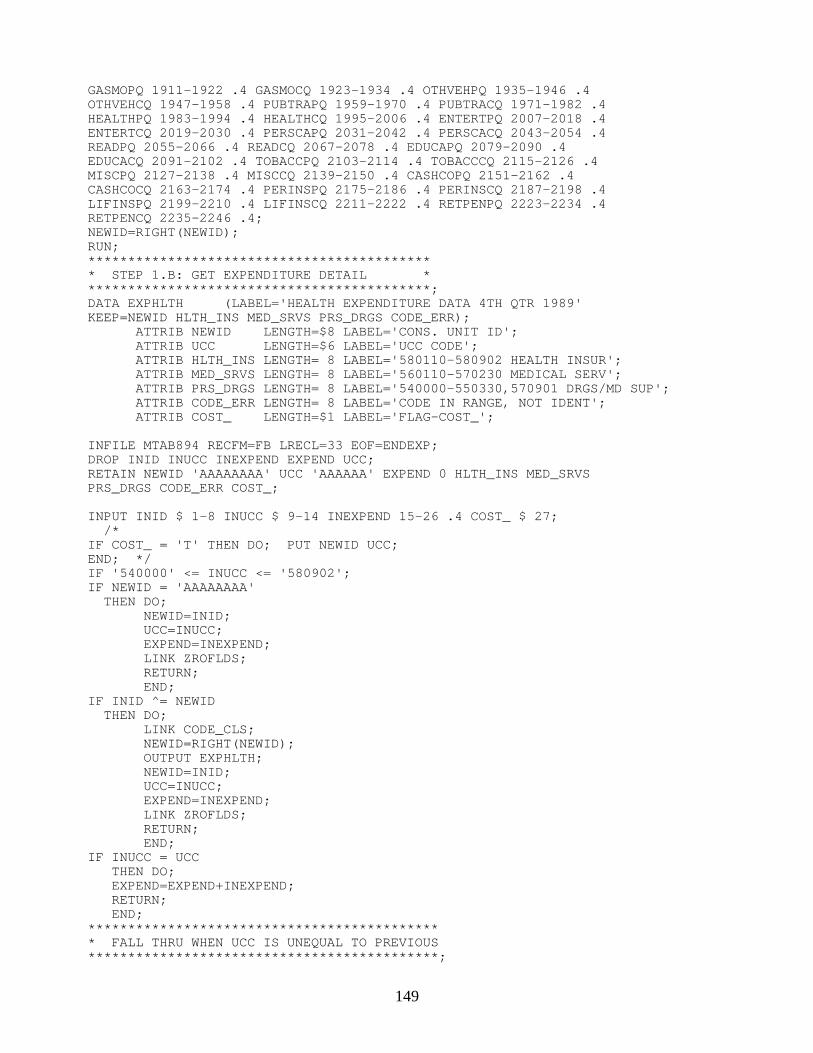
149

GASMOPQ 1911-1922 .4 GASMOCQ 1923-1934 .4 OTHVEHPQ 1935-1946 .4OTHVEHCQ 1947-1958 .4 PUBTRAPQ 1959-1970 .4 PUBTRACQ 1971-1982 .4HEALTHPQ 1983-1994 .4 HEALTHCQ 1995-2006 .4 ENTERTPQ 2007-2018 .4ENTERTCQ 2019-2030 .4 PERSCAPQ 2031-2042 .4 PERSCACQ 2043-2054 .4READPQ 2055-2066 .4 READCQ 2067-2078 .4 EDUCAPQ 2079-2090 .4EDUCACQ 2091-2102 .4 TOBACCPQ 2103-2114 .4 TOBACCCQ 2115-2126 .4MISCPQ 2127-2138 .4 MISCCQ 2139-2150 .4 CASHCOPQ 2151-2162 .4CASHCOCQ 2163-2174 .4 PERINSPQ 2175-2186 .4 PERINSCQ 2187-2198 .4LIFINSPQ 2199-2210 .4 LIFINSCQ 2211-2222 .4 RETPENPQ 2223-2234 .4RETPENCQ 2235-2246 .4;NEWID=RIGHT(NEWID);RUN;******************************************** STEP 1.B: GET EXPENDITURE DETAIL ********************************************;DATA EXPHLTH (LABEL='HEALTH EXPENDITURE DATA 4TH QTR 1989'KEEP=NEWID HLTH_INS MED_SRVS PRS_DRGS CODE_ERR); ATTRIB NEWID LENGTH=$8 LABEL='CONS. UNIT ID'; ATTRIB UCC LENGTH=$6 LABEL='UCC CODE'; ATTRIB HLTH_INS LENGTH= 8 LABEL='580110-580902 HEALTH INSUR'; ATTRIB MED_SRVS LENGTH= 8 LABEL='560110-570230 MEDICAL SERV'; ATTRIB PRS_DRGS LENGTH= 8 LABEL='540000-550330,570901 DRGS/MD SUP'; ATTRIB CODE_ERR LENGTH= 8 LABEL='CODE IN RANGE, NOT IDENT'; ATTRIB COST_ LENGTH=$1 LABEL='FLAG-COST_'; INFILE MTAB894 RECFM=FB LRECL=33 EOF=ENDEXP;DROP INID INUCC INEXPEND EXPEND UCC;RETAIN NEWID 'AAAAAAAA' UCC 'AAAAAA' EXPEND 0 HLTH_INS MED_SRVSPRS_DRGS CODE_ERR COST_; INPUT INID $ 1-8 INUCC $ 9-14 INEXPEND 15-26 .4 COST_ $ 27; /*IF COST_ = 'T' THEN DO; PUT NEWID UCC;END; */IF '540000' <= INUCC <= '580902';IF NEWID = 'AAAAAAAA' THEN DO; NEWID=INID; UCC=INUCC; EXPEND=INEXPEND; LINK ZROFLDS; RETURN; END;IF INID ^= NEWID THEN DO; LINK CODE_CLS; NEWID=RIGHT(NEWID); OUTPUT EXPHLTH; NEWID=INID; UCC=INUCC; EXPEND=INEXPEND; LINK ZROFLDS; RETURN; END;IF INUCC = UCC THEN DO; EXPEND=EXPEND+INEXPEND; RETURN; END;********************************************* FALL THRU WHEN UCC IS UNEQUAL TO PREVIOUS********************************************;

150

LINK CODE_CLS;EXPEND=INEXPEND;UCC=INUCC;RETURN;********************************************* EXECUTE FOLLOWING AT END OF FILE *********************************************;ENDEXP:LINK CODE_CLS;NEWID=RIGHT(NEWID);OUTPUT EXPHLTH;RETURN;************************************** ZERO EXPENDITURE ACCUMULATORS **************************************;ZROFLDS:HLTH_INS = 0; MED_SRVS = 0; PRS_DRGS = 0; CODE_ERR = 0;RETURN;************************************** ADD UNIT'S EXPENSE TO ACCUMULATOR**************************************;CODE_CLS:IF UCC = '580110' OR UCC = '580210' OR UCC = '580310' OR UCC = '580901' OR UCC = '580902' THEN DO; HLTH_INS = HLTH_INS + EXPEND; RETURN; END;IF UCC = '560110' OR UCC = '560210' OR UCC = '560310' OR UCC = '560320' OR UCC = '560330' OR UCC = '560900' OR UCC = '570110' OR UCC = '570210' OR UCC = '570220' OR UCC = '570230' THEN DO; MED_SRVS = MED_SRVS + EXPEND; RETURN; END;IF UCC = '540000' OR UCC = '550110' OR UCC = '550320' OR UCC = '550330' OR UCC = '570901' THEN DO; PRS_DRGS = PRS_DRGS + EXPEND; RETURN; END;******************************************************** IN UNLIKELY CASE THAT CODE IS UNMATCHED, ADD TO ** SPECIAL ACCUMULATOR ********************************************************;CODE_ERR=CODE_ERR+EXPEND; RETURN;RUN;/*DATA;SET;IF CODE_ERR ^= 0 THEN DO;PUT NEWID HLTH_INS MED_SRVS PRS_DRGS CODE_ERR;END; */****************************************************** AGGREGATING FOOD EXPENDITURE. ******************************************************;DATA EXPFOOD (LABEL='FOOD EXPENDITURE'KEEP=NEWID FOOD_HOM FOOD_AWY CODE_FUD); ATTRIB NEWID LENGTH=$8 LABEL='CONS. UNIT ID'; ATTRIB UCC LENGTH=$6 LABEL='UCC CODE'; ATTRIB FOOD_HOM LENGTH=8 LABEL='FOOD AT HOME'; ATTRIB FOOD_AWY LENGTH=6 LABEL='FOOD AWAY FROM HOME'; ATTRIB CODE_FUD LENGTH=8 LABEL='CODE IN RANGE, NOT IDENT'; ATTRIB COST_ LENGTH=$1 LABEL='FLAG-COST_';INFILE MTAB894 RECFM=FB LRECL=33 EOF=ENDEXP;DROP FDID FDUCC FDEXPEND EXPEND UCC;RETAIN NEWID 'AAAAAAAA' UCC 'AAAAAA' EXPEND 0 FOOD_HOM FOOD_AWY CODE_FUDCOST_;INPUT FDID $ 1-8 FDUCC $ 9-14 FDEXPEND 15-26 .4 COST_ $ 27; /*IF COST_ = 'T' THEN DO; PUT NEWID UCC;

151

END; */IF '190901'<= FDUCC <= '190904'OR '790220'<= FDUCC <= '790230'OR FDUCC = '790430'OR FDUCC = '790410'OR FDUCC = '800700';IF NEWID = 'AAAAAAAA' THEN DO;NEWID=FDID;UCC=FDUCC;EXPEND=FDEXPEND;LINK ZROFLDS;RETURN;END;IF FDID ^= NEWID THEN DO;LINK CODE_CLS;NEWID=RIGHT(NEWID);OUTPUT EXPFOOD;NEWID=FDID;UCC=FDUCC;EXPEND=FDEXPEND;LINK ZROFLDS;RETURN; END;IF FDUCC = UCC THEN DO; EXPEND=EXPEND+FDEXPEND; RETURN; END;LINK CODE_CLS;EXPEND=FDEXPEND;UCC=FDUCC;RETURN;ENDEXP:LINK CODE_CLS;NEWID=RIGHT(NEWID);OUTPUT EXPFOOD;RETURN;ZROFLDS:FOOD_HOM=0; FOOD_AWY=0; CODE_FUD=0;RETURN;CODE_CLS:IF UCC = '190904' OR UCC = '790220' OR UCC = '790230' THEN DO;FOOD_HOM = FOOD_HOM + EXPEND;RETURN;END;IF UCC = '190901' OR UCC = '190902' OR UCC = '190903' OR UCC = '790410' OR UCC = '800700' OR UCC = '790430' THEN DO;FOOD_AWY =FOOD_AWY + EXPEND;RETURN;END;CODE_FUD = CODE_FUD +EXPEND;RETURN;RUN; /*DATA;SET;IF CODE_FUD ^= 0 THEN DO;PUT NEWID FOOD_HOM FOOD_AWY CODE_FUD;END; */****************************************************** AGGREGATING EXPENDITURE FOR ALCOHOLIC BEVERAGES ******************************************************;DATA EXPBEVER (LABEL='ALCOHOL EXPENDITURE'KEEP=NEWID ALCH_BVG CODE_BVG);

152

ATTRIB NEWID LENGTH=$8 LABEL='CONS. UNIT ID'; ATTRIB UCC LENGTH=$6 LABEL='UCC CODE'; ATTRIB ALCH_BVG LENGTH=8 LABEL='ALCHOLIC BEVERAGES'; ATTRIB CODE_BVG LENGTH=8 LABEL='CODE IN RANGE, NOT IDENT'; ATTRIB COST_ LENGTH=$1 LABEL='FLAG-COST_';INFILE MTAB894 RECFM=FB LRECL=33 EOF=ENDEXP;DROP ALID ALUCC ALEXPEND EXPEND UCC;RETAIN NEWID 'AAAAAAAA' UCC 'AAAAAA' EXPEND 0 ALCH_BVG CODE_BVG COST_;INPUT ALID $ 1-8 ALUCC $ 9-14 ALEXPEND 15-26 .4 COST_ $ 27; /*IF COST_ = 'T' THEN DO; PUT NEWID UCC;END; */IF ALUCC = '200900'OR ALUCC = '790310'OR ALUCC = '790320'OR ALUCC = '790420';IF NEWID = 'AAAAAAAA' THEN DO;NEWID=ALID;UCC=ALUCC;EXPEND=ALEXPEND;LINK ZROFLDS;RETURN;END;IF ALID ^= NEWID THEN DO;LINK CODE_CLS;NEWID=RIGHT(NEWID);OUTPUT EXPBEVER;NEWID=ALID;UCC=ALUCC;EXPEND=ALEXPEND;LINK ZROFLDS;RETURN; END;IF ALUCC = UCC THEN DO; EXPEND=EXPEND+ALEXPEND; RETURN; END;LINK CODE_CLS;EXPEND=ALEXPEND;UCC=ALUCC;RETURN;ENDEXP:LINK CODE_CLS;NEWID=RIGHT(NEWID);OUTPUT EXPBEVER;RETURN;ZROFLDS:ALCH_BVG=0; CODE_BVG=0;RETURN;CODE_CLS:IF UCC = '200900' OR UCC = '790310' OR UCC = '790320' OR UCC = '790420' THEN DO;ALCH_BVG = ALCH_BVG + EXPEND;RETURN; END;CODE_BVG = CODE_BVG + EXPEND;RETURN;RUN; /*DATA;SET;IF CODE_BVG ^= 0 THEN DO;PUT NEWID ALCH_BVG CODE_BVG;END; */

153

****************************************************** AGGREGATING HOUSING EXPENDITURE. ******************************************************;DATA EXPHOUS (LABEL='HOUSING EXPENDITURE'KEEP=NEWID OWND_DWL RENT_DWL OTHR_DWL CODE_DWL); ATTRIB NEWID LENGTH=$8 LABEL='CONS. UNIT ID'; ATTRIB UCC LENGTH=$6 LABEL='UCC CODE'; ATTRIB OWND_DWL LENGTH=8 LABEL='OWNED DWELLING'; ATTRIB RENT_DWL LENGTH=8 LABEL='RENTED DWELLING'; ATTRIB OTHR_DWL LENGTH=8 LABEL='OTHER LODGING'; ATTRIB CODE_DWL LENGTH=8 LABEL='CODE IN RANGE, NOT IDENT'; ATTRIB COST_ LENGTH=$1 LABEL='FLAG-COST_';INFILE MTAB894 RECFM=FB LRECL=33 EOF=ENDEXP;DROP HSID HSUCC HSEXPEND EXPEND UCC;RETAIN NEWID 'AAAAAAAA' UCC 'AAAAAA' EXPEND 0 OWND_DWL RENT_DWL OTHR_DWLCODE_DWL COST_;INPUT HSID $ 1-8 HSUCC $ 9-14 HSEXPEND 15-26 .4 COST_ $ 27; /*IF COST_ = 'T' THEN DO; PUT NEWID UCC;END; */IF '210110' <= HSUCC <= '220322'OR '220901' <= HSUCC <= '270214'OR '270411' <= HSUCC <= '300412'OR '320110' <= HSUCC <= '340530'OR '340620' <= HSUCC <= '340901'OR '340903' <= HSUCC <= '340904'OR '340906' <= HSUCC <= '350110'OR HSUCC = '430130'OR HSUCC = '670310'OR '690110' <= HSUCC <= '690245'OR HSUCC = '790600'OR HSUCC = '790690'OR HSUCC = '800710'OR '990900' <= HSUCC <= '990950';IF NEWID = 'AAAAAAAA' THEN DO;NEWID=HSID;UCC=HSUCC;EXPEND=HSEXPEND;LINK ZROFLDS;RETURN;END;IF HSID ^= NEWID THEN DO;LINK CODE_CLS;NEWID=RIGHT(NEWID);OUTPUT EXPHOUS;NEWID=HSID;UCC=HSUCC;EXPEND=HSEXPEND;LINK ZROFLDS;RETURN; END;IF HSUCC = UCC THEN DO; EXPEND=EXPEND+HSEXPEND; RETURN; END;LINK CODE_CLS;EXPEND=HSEXPEND;UCC=HSUCC;RETURN;ENDEXP:

154

LINK CODE_CLS;NEWID=RIGHT(NEWID);OUTPUT EXPHOUS;RETURN;ZROFLDS:OWND_DWL=0; RENT_DWL=0; OTHR_DWL=0; CODE_DWL=0;RETURN;CODE_CLS:IF UCC = '220311' OR UCC = '220321' OR UCC = '220211' OR UCC = '230901'OR UCC = '340911' OR UCC = '220121' OR UCC = '220111' OR UCC = '210901'OR UCC = '230112' OR UCC = '230113' OR UCC = '230114' OR UCC = '230115'OR UCC = '230116' OR UCC = '220901' OR UCC = '230122' OR UCC = '230142'OR UCC = '240112' OR UCC = '240122' OR UCC = '240312' OR UCC = '240322'OR UCC = '320622' OR UCC = '240212' OR UCC = '240213' OR UCC = '240222'OR UCC = '320632' OR UCC = '320612' OR UCC = '990930' THEN DO;OWND_DWL = OWND_DWL + EXPEND;RETURN;END;IF UCC = '230111' OR UCC = '230121' OR UCC = '230141' OR UCC = '350110'OR UCC = '240111' OR UCC = '240121' OR UCC = '240211' OR UCC = '240221'OR UCC = '240311' OR UCC = '240321' OR UCC = '320611' OR UCC = '990910'OR UCC = '990920' OR UCC = '790690' OR UCC = '320621' OR UCC = '320631'OR UCC = '210110' OR UCC = '800710'OR UCC = '990950' THEN DO;RENT_DWL =RENT_DWL + EXPEND;RETURN;END;IF UCC = '220212' OR UCC = '220122' OR UCC = '220112' OR UCC = '210902'OR UCC = '230119' OR UCC = '230123' OR UCC = '240113' OR UCC = '240123'OR UCC = '240214' OR UCC = '240223' OR UCC = '240313' OR UCC = '240323'OR UCC = '320613' OR UCC = '990940' OR UCC = '320623' OR UCC = '320633'OR UCC = '230902' OR UCC = '340912' OR UCC = '220902' OR UCC = '790600'OR UCC = '220322' OR UCC = '220312' OR UCC = '210310' OR UCC = '210210' THEN DO;OTHR_DWL =OTHR_DWL + EXPEND;RETURN;END;CODE_DWL = CODE_DWL +EXPEND;RETURN;RUN; /*DATA;SET;IF CODE_DWL ^= 0 THEN DO;PUT NEWID OWND_DWL RENT_DWL OTHR_DWL CODE_DWL;END; */****************************************************** AGGREGATING EXPENDITURE ON UTILITY ******************************************************;DATA EXPUTIL (LABEL='UTILITY EXPENDITURE'KEEP=NEWID NATL_GAS ELEC_ITY FUEL_OIL TELE_PHN WATR_PLS CODE_UTL); ATTRIB NEWID LENGTH=$8 LABEL='CONS. UNIT ID'; ATTRIB UCC LENGTH=$6 LABEL='UCC CODE'; ATTRIB NATL_GAS LENGTH=8 LABEL='NATURAL GAS'; ATTRIB ELEC_ITY LENGTH=8 LABEL='ELECTRICITY'; ATTRIB FUEL_OIL LENGTH=8 LABEL='FUEL OIL'; ATTRIB TELE_PHN LENGTH=8 LABEL='TELEPHONE'; ATTRIB WATR_PLS LENGTH=8 LABEL='WATER AND OTHER SERVICES'; ATTRIB CODE_UTL LENGTH=8 LABEL='CODE IN RANGE, NOT IDENT'; ATTRIB COST_ LENGTH=$1 LABEL='FLAG-COST_';INFILE MTAB894 RECFM=FB LRECL=33 EOF=ENDEXP;DROP UTID UTUCC UTEXPEND EXPEND UCC;RETAIN NEWID 'AAAAAAAA' UCC 'AAAAAA' EXPEND 0 NATL_GAS ELEC_ITY FUEL_OILTELE_PHN WATR_PLS CODE_UTL COST_;

155

INPUT UTID $ 1-8 UTUCC $ 9-14 UTEXPEND 15-26 .4 COST_ $ 27; /*IF COST_ = 'T' THEN DO; PUT NEWID UCC;END; */IF '250111' <= UTUCC <= '270214'OR '270411' <= UTUCC <= '270904';IF NEWID = 'AAAAAAAA' THEN DO;NEWID=UTID;UCC=UTUCC;EXPEND=UTEXPEND;LINK ZROFLDS;RETURN;END;IF UTID ^= NEWID THEN DO;LINK CODE_CLS;NEWID=RIGHT(NEWID);OUTPUT EXPUTIL;NEWID=UTID;UCC=UTUCC;EXPEND=UTEXPEND;LINK ZROFLDS;RETURN; END;IF UTUCC = UCC THEN DO; EXPEND=EXPEND+UTEXPEND; RETURN; END;LINK CODE_CLS;EXPEND=UTEXPEND;UCC=UTUCC;RETURN;ENDEXP:LINK CODE_CLS;NEWID=RIGHT(NEWID);OUTPUT EXPUTIL;RETURN;ZROFLDS:NATL_GAS=0; ELEC_ITY=0; FUEL_OIL=0; TELE_PHN=0; WATR_PLS=0; CODE_UTL=0;RETURN;CODE_CLS:IF UCC = '260211' OR UCC = '260212' OR UCC = '260213' OR UCC = '260214' THEN DO;NATL_GAS = NATL_GAS + EXPEND;RETURN;END;IF UCC = '260111' OR UCC = '260112' OR UCC = '260113' OR UCC = '260114' THEN DO;ELEC_ITY =ELEC_ITY + EXPEND;RETURN;END;IF UCC = '250111' OR UCC = '250112' OR UCC = '250113' OR UCC = '250114'OR UCC = '250211' OR UCC = '250212' OR UCC = '250213' OR UCC = '250214'OR UCC = '250221' OR UCC = '250222' OR UCC = '250223' OR UCC = '250224'OR UCC = '250901' OR UCC = '250902' OR UCC = '250903' OR UCC = '250904' THEN DO;FUEL_OIL = FUEL_OIL + EXPEND;RETURN;END;IF UCC = '270000' THEN DO;

156

TELE_PHN = TELE_PHN + EXPEND;RETURN;END;IF UCC = '270211' OR UCC = '270212' OR UCC = '270213' OR UCC = '270214'OR UCC = '270411' OR UCC = '270412' OR UCC = '270413' OR UCC = '270414'OR UCC = '270901' OR UCC = '270902' OR UCC = '270903' OR UCC = '270904' THEN DO;WATR_PLS + WATR_PLS + EXPEND;RETURN;END;CODE_UTL = CODE_UTL +EXPEND;RETURN;RUN; /*DATA;SET;IF CODE_UTL ^= 0 THEN DO;PUT NEWID NATL_GAS ELEC_ITY FUEL_OIL TELE_PHN WATR_PLS CODE_UTL;END; */****************************************************** AGGREGATING EXPENDITURE ON HOUSEHOLD OPERATION. ******************************************************;DATA EXPHHOLD (LABEL='HOUSEHOL OPERATION EXPENDITURE'KEEP=NEWID DOME_SER OTHR_SER CODE_SER); ATTRIB NEWID LENGTH=$8 LABEL='CONS. UNIT ID'; ATTRIB UCC LENGTH=$6 LABEL='UCC CODE'; ATTRIB DOME_SER LENGTH=8 LABEL='DOMESTIC SERVICES'; ATTRIB OTHR_SER LENGTH=8 LABEL='OTHER HOUSEHOLD EXPENSES'; ATTRIB CODE_SER LENGTH=8 LABEL='CODE IN RANGE, NOT IDENT'; ATTRIB COST_ LENGTH=$1 LABEL='FLAG-COST_';INFILE MTAB894 RECFM=FB LRECL=33 EOF=ENDEXP;DROP HHID HHUCC HHEXPEND EXPEND UCC;RETAIN NEWID 'AAAAAAAA' UCC 'AAAAAA' EXPEND 0 DOME_SER OTHR_SER CODE_SERCOST_;INPUT HHID $ 1-8 HHUCC $ 9-14 HHEXPEND 15-26 .4 COST_ $ 27; /*IF COST_ = 'T' THEN DO; PUT NEWID UCC;END; */IF HHUCC = '330511'OR '340210' <= HHUCC <= '340530'OR '340620' <= HHUCC <= '340901'OR HHUCC = '340903'OR '340906' <= HHUCC <= '340908'OR HHUCC = '670310'OR HHUCC = '990900'OR HHUCC = '690113';IF NEWID = 'AAAAAAAA' THEN DO;NEWID=HHID;UCC=HHUCC;EXPEND=HHEXPEND;LINK ZROFLDS;RETURN;END;IF HHID ^= NEWID THEN DO;LINK CODE_CLS;NEWID=RIGHT(NEWID);OUTPUT EXPHHOLD;NEWID=HHID;UCC=HHUCC;EXPEND=HHEXPEND;LINK ZROFLDS;RETURN; END;IF HHUCC = UCC THEN DO;

157

EXPEND=EXPEND+HHEXPEND; RETURN; END;LINK CODE_CLS;EXPEND=HHEXPEND;UCC=HHUCC;RETURN;ENDEXP:LINK CODE_CLS;NEWID=RIGHT(NEWID);OUTPUT EXPHHOLD;RETURN;ZROFLDS:DOME_SER=0; OTHR_SER=0; CODE_SER=0;RETURN;CODE_CLS:IF UCC = '340210' OR UCC = '340310' OR UCC = '340410' OR UCC = '340420'OR UCC = '340520' OR UCC = '340530' OR UCC = '340903' OR UCC = '340906'OR UCC = '670310' THEN DO;DOME_SER = DOME_SER + EXPEND;RETURN;END;IF UCC = '330511' OR UCC = '340510' OR UCC = '340620' OR UCC = '340630'OR UCC = '340901' OR UCC = '990900' OR UCC = '340907' OR UCC = '340908'OR UCC = '690113' THEN DO;OTHR_SER = OTHR_SER + EXPEND;RETURN;END;CODE_SER = CODE_SER +EXPEND;RETURN;RUN; /*DATA;SET;IF CODE_SER ^= 0 THEN DO;PUT NEWID DOME_SER OTHR_SER CODE_SER;END; */****************************************************** AGGREGATING EXPENDITURE ON HOUSEFURNISHING. ******************************************************;DATA EXPFURN (LABEL='HOUSEFURNISHING EXPENDITURE'KEEP=NEWID HOUS_FUR CODE_FUR); ATTRIB NEWID LENGTH=$8 LABEL='CONS. UNIT ID'; ATTRIB UCC LENGTH=$6 LABEL='UCC CODE'; ATTRIB HOUS_FUR LENGTH=8 LABEL='HOUSEFURNISHINGS'; ATTRIB CODE_FUR LENGTH=8 LABEL='CODE IN RANGE, NOT IDENT'; ATTRIB COST_ LENGTH=$1 LABEL='FLAG-COST_';INFILE MTAB894 RECFM=FB LRECL=33 EOF=ENDEXP;DROP HFID HFUCC HFEXPEND EXPEND UCC;RETAIN NEWID 'AAAAAAAA' UCC 'AAAAAA' EXPEND 0 HOUS_FUR CODE_FUR COST_;INPUT HFID $ 1-8 HFUCC $ 9-14 HFEXPEND 15-26 .4 COST_ $ 27; /*IF COST_ = 'T' THEN DO; PUT NEWID UCC;END; */IF '230117' <= HFUCC <= '230118'OR '230131' <= HFUCC <= '230132'OR '280110' <= HFUCC <= '300412'OR '320110' <= HFUCC <= '320522'OR '320901' <= HFUCC <= '320904'OR HFUCC <= '340904'OR HFUCC <= '430130'OR '690110' <= HFUCC <= '690230';IF NEWID = 'AAAAAAAA' THEN DO;

158

NEWID=HFID;UCC=HFUCC;EXPEND=HFEXPEND;LINK ZROFLDS;RETURN;END;IF HFID ^= NEWID THEN DO;LINK CODE_CLS;NEWID=RIGHT(NEWID);OUTPUT EXPFURN;NEWID=HFID;UCC=HFUCC;EXPEND=HFEXPEND;LINK ZROFLDS;RETURN; END;IF HFUCC = UCC THEN DO; EXPEND=EXPEND+HFEXPEND; RETURN; END;LINK CODE_CLS;EXPEND=HFEXPEND;UCC=HFUCC;RETURN;ENDEXP:LINK CODE_CLS;NEWID=RIGHT(NEWID);OUTPUT EXPFURN;RETURN;ZROFLDS:HOUS_FUR=0; CODE_FUR=0;RETURN;CODE_CLS:IF UCC = '280110' OR UCC = '280120' OR UCC = '280130' OR UCC = '280210'OR UCC = '280220' OR UCC = '280230' OR UCC = '280900' OR UCC = '290110'OR UCC = '290120' OR UCC = '290210' OR UCC = '290310' OR UCC = '290320'OR UCC = '290410' OR UCC = '290420' OR UCC = '290430' OR UCC = '290440'OR UCC = '300111' OR UCC = '300112' OR UCC = '300211' OR UCC = '300212'OR UCC = '300221' OR UCC = '300222' OR UCC = '300311' OR UCC = '300312'OR UCC = '300321' OR UCC = '300322' OR UCC = '300331' OR UCC = '300332'OR UCC = '300411' OR UCC = '300412' OR UCC = '230131' OR UCC = '230132'OR UCC = '320110' OR UCC = '320120' OR UCC = '320130' OR UCC = '320150'OR UCC = '320161' OR UCC = '320162' OR UCC = '320210' OR UCC = '320220'OR UCC = '320231' OR UCC = '320232' OR UCC = '320310' OR UCC = '320320'OR UCC = '320330' OR UCC = '320340' OR UCC = '320350' OR UCC = '320360'OR UCC = '320370' OR UCC = '320410' OR UCC = '320420' OR UCC = '320511'OR UCC = '320512' OR UCC = '320521' OR UCC = '320522' OR UCC = '230117'OR UCC = '230118' OR UCC = '340904' OR UCC = '690210' OR UCC = '690210'OR UCC = '690220' OR UCC = '690230'OR UCC = '430130' OR UCC = '320901' OR UCC = '320902' OR UCC = '320903'OR UCC = '320904' THEN DO;HOUS_FUR = HOUS_FUR + EXPEND;RETURN;END;CODE_FUR = CODE_FUR +EXPEND;RETURN;RUN; /*DATA;SET;IF CODE_FUR ^= 0 THEN DO;PUT NEWID HOUS_FUR CODE_FUR;END;*/*****************************************************

159

* AGGREGATING EXPENDITURE ON APPAREL AND SERVICES. ******************************************************;DATA EXPAPRL (LABEL='APPAREL EXPENDITURE'KEEP=NEWID BOYS_MEN WOME_GIR CHIL_TWO FOOT_WER OTHR_APP CODE_APP); ATTRIB NEWID LENGTH=$8 LABEL='CONS. UNIT ID'; ATTRIB UCC LENGTH=$6 LABEL='UCC CODE'; ATTRIB BOYS_MEN LENGTH=8 LABEL='MEN AND BOYS'; ATTRIB WOME_GIR LENGTH=8 LABEL='WOMEN AND GIRLS'; ATTRIB CHIL_TWO LENGTH=8 LABEL='CHILDREN UNDER TWO'; ATTRIB FOOT_WER LENGTH=8 LABEL='FOOTWEAR'; ATTRIB OTHR_APP LENGTH=8 LABEL='OTHER APPAREL PRODUCTS'; ATTRIB CODE_APP LENGTH=8 LABEL='CODE IN RANGE, NOT IDENT'; ATTRIB COST_ LENGTH=$1 LABEL='FLAG-COST_';INFILE MTAB894 RECFM=FB LRECL=33 EOF=ENDEXP;DROP APID APUCC APEXPEND EXPEND UCC;RETAIN NEWID 'AAAAAAAA' UCC 'AAAAAA' EXPEND 0 BOYS_MEN WOME_GIR CHIL_TWOFOOT_WER OTHR_APP CODE_APP COST_;INPUT APID $ 1-8 APUCC $ 9-14 APEXPEND 15-26 .4 COST_ $ 27; /*IF COST_ = 'T' THEN DO; PUT NEWID UCC;END; */IF '360110' <= APUCC <= '430120'OR '440110' <= APUCC <= '440900';IF NEWID = 'AAAAAAAA' THEN DO;NEWID=APID;UCC=APUCC;EXPEND=APEXPEND;LINK ZROFLDS;RETURN;END;IF APID ^= NEWID THEN DO;LINK CODE_CLS;NEWID=RIGHT(NEWID);OUTPUT EXPAPRL;NEWID=APID;UCC=APUCC;EXPEND=APEXPEND;LINK ZROFLDS;RETURN; END;IF APUCC = UCC THEN DO; EXPEND=EXPEND+APEXPEND; RETURN; END;LINK CODE_CLS;EXPEND=APEXPEND;UCC=APUCC;RETURN;ENDEXP:LINK CODE_CLS;NEWID=RIGHT(NEWID);OUTPUT EXPAPRL;RETURN;ZROFLDS:BOYS_MEN=0; WOME_GIR=0; CHIL_TWO=0; FOOT_WER=0; OTHR_APP=0; CODE_APP=0;RETURN;CODE_CLS:IF UCC = '360110' OR UCC = '360120' OR UCC = '360210' OR UCC = '360311'OR UCC = '360312' OR UCC = '360320' OR UCC = '360330' OR UCC = '360340'OR UCC = '360350' OR UCC = '360410' OR UCC = '360511' OR UCC = '360512'

160

OR UCC = '360901' OR UCC = '360902' OR UCC = '370110' OR UCC = '370120'OR UCC = '370130' OR UCC = '370211' OR UCC = '370212' OR UCC = '370213'OR UCC = '370220' OR UCC = '370311' OR UCC = '370312' OR UCC = '370313'OR UCC = '370901' OR UCC = '370902' THEN DO;BOYS_MEN = BOYS_MEN + EXPEND;RETURN;END;IF UCC = '380110' OR UCC = '380210' OR UCC = '380311' OR UCC = '380312'OR UCC = '380313' OR UCC = '380320' OR UCC = '380331' OR UCC = '380332'OR UCC = '380340' OR UCC = '380410' OR UCC = '380420' OR UCC = '380430'OR UCC = '380510' OR UCC = '380901' OR UCC = '380902' OR UCC = '380903'OR UCC = '390110' OR UCC = '390120' OR UCC = '390210' OR UCC = '390221'OR UCC = '390222' OR UCC = '390230' OR UCC = '390310' OR UCC = '390321'OR UCC = '390322' OR UCC = '390901' OR UCC = '390902' THEN DO;WOME_GIR =WOME_GIR + EXPEND;RETURN;END;IF UCC = '410111' OR UCC = '410112' OR UCC = '410121' OR UCC = '410122'OR UCC = '410131' OR UCC = '410132' OR UCC = '410141' OR UCC = '410142'OR UCC = '410901' OR UCC = '410902' OR UCC = '410903' OR UCC = '410904' THEN DO;CHIL_TWO = CHIL_TWO + EXPEND;RETURN;END;IF UCC = '400110' OR UCC = '400210' OR UCC = '400220' OR UCC = '400310' THEN DO;FOOT_WER = FOOT_WER + EXPEND;RETURN;END;IF UCC = '420110' OR UCC = '420120' OR UCC = '430110' OR UCC = '430120'OR UCC = '440110' OR UCC = '440120' OR UCC = '440130' OR UCC = '440140'OR UCC = '440150' OR UCC = '440210' OR UCC = '440900' THEN DO;OTHR_APP = OTHR_APP + EXPEND;RETURN;END;CODE_APP = CODE_APP +EXPEND;RETURN;RUN; /*DATA;SET;IF CODE_APP ^= 0 THEN DO;PUT NEWID BOYS_MEN WOME_GIR CHIL_TWO FOOT_WER OTHR_APP CODE_APP;END; */****************************************************** AGGREGATING EXPENDITURE ON TRANSPORTATION. ******************************************************;DATA EXPTRANS (LABEL='TRANSPORT EXPENDITURE'KEEP=NEWID NCAR_TRC UCAR_TRC OTHR_VCL VHCL_FIN GALN_OIL MAIN_RPR VHCL_INS PUBL_TRA VHCL_RET CODE_TRA); ATTRIB NEWID LENGTH=$8 LABEL='CONS. UNIT ID'; ATTRIB UCC LENGTH=$6 LABEL='UCC CODE'; ATTRIB NCAR_TRC LENGTH=8 LABEL='NEW CARS AND TRUCKS'; ATTRIB UCAR_TRC LENGTH=8 LABEL='USED CARS AND TRUCKS'; ATTRIB OTHR_VCL LENGTH=8 LABEL='OTHER VEHICLES'; ATTRIB VHCL_FIN LENGTH=8 LABEL='VEHICLE FINANCE CHARGES'; ATTRIB GALN_OIL LENGTH=8 LABEL='GASOLINE AND OIL'; ATTRIB MAIN_RPR LENGTH=8 LABEL='MAINTENANCE AND REPAIRS'; ATTRIB VHCL_INS LENGTH=8 LABEL='VEHICLE INSURANCE'; ATTRIB PUBL_TRA LENGTH=8 LABEL='PUBLIC TRANSPORTATION'; ATTRIB VHCL_RET LENGTH=8 LABEL='VEHICLE RENTAL'; ATTRIB CODE_TRA LENGTH=8 LABEL='CODE IN RANGE, NOT IDENT';

161

ATTRIB COST_ LENGTH=$1 LABEL='FLAG-COST_';INFILE MTAB894 RECFM=FB LRECL=33 EOF=ENDEXP;DROP TRID TRUCC TREXPEND EXPEND UCC;RETAIN NEWID 'AAAAAAAA' UCC 'AAAAAA' EXPEND 0 NCAR_TRC UCAR_TRC OTHR_VCLVHCL_FIN GALN_OIL MAIN_RPR VHCL_INS PUBL_TRA VHCL_RET CODE_TRA COST_;INPUT TRID $ 1-8 TRUCC $ 9-14 TREXPEND 15-26 .4 COST_ $ 27; /*IF COST_ = 'T' THEN DO; PUT NEWID UCC;END; */IF TRUCC = '450110'OR TRUCC = '450210'OR TRUCC = '450220'OR TRUCC = '460110'OR TRUCC = '450900'OR '460901' <= TRUCC <= '460903'OR '470111' <= TRUCC <= '470212'OR '470220' <= TRUCC <= '530902'OR '620906' <= TRUCC <= '620907'OR TRUCC = '850300'OR TRUCC = '620902';IF NEWID = 'AAAAAAAA' THEN DO;NEWID=TRID;UCC=TRUCC;EXPEND=TREXPEND;LINK ZROFLDS;RETURN;END;IF TRID ^= NEWID THEN DO;LINK CODE_CLS;NEWID=RIGHT(NEWID);OUTPUT EXPTRANS;NEWID=TRID;UCC=TRUCC;EXPEND=TREXPEND;LINK ZROFLDS;RETURN; END;IF TRUCC = UCC THEN DO; EXPEND=EXPEND+TREXPEND; RETURN; END;LINK CODE_CLS;EXPEND=TREXPEND;UCC=TRUCC;RETURN;ENDEXP:LINK CODE_CLS;NEWID=RIGHT(NEWID);OUTPUT EXPTRANS;RETURN;ZROFLDS:NCAR_TRC=0; UCAR_TRC=0; OTHR_VCL=0; VHCL_FIN=0; GALN_OIL=0; MAIN_RPR=0;VHCL_INS=0; PUBL_TRA=0; VHCL_RET=0; CODE_TRA=0;RETURN;CODE_CLS:IF UCC = '450110' OR UCC = '450210' THEN DO;NCAR_TRC = NCAR_TRC + EXPEND;RETURN;END;

162

IF UCC = '460110' OR UCC = '460901' THEN DO;UCAR_TRC =UCAR_TRC + EXPEND;RETURN;END;IF UCC = '450900' OR UCC = '460902' OR UCC = '460903' THEN DO;OTHR_VCL = OTHR_VCL + EXPEND;RETURN;END;IF UCC = '510110' OR UCC = '510901' OR UCC = '510902' OR UCC = '850300' THEN DO;VHCL_FIN = VHCL_FIN + EXPEND;RETURN;END;IF UCC = '470111' OR UCC = '470112' OR UCC = '470113' OR UCC = '470211'OR UCC = '470212' THEN DO;GALN_OIL = GALN_OIL + EXPEND;RETURN;END;IF UCC = '470220' OR UCC = '480110' OR UCC = '480211' OR UCC = '490110'OR UCC = '490211' OR UCC = '490212' OR UCC = '490220' OR UCC = '490231'OR UCC = '490232' OR UCC = '490311' OR UCC = '490312' OR UCC = '490313'OR UCC = '490314' OR UCC = '490315' OR UCC = '490317' OR UCC = '490318'OR UCC = '490411' OR UCC = '490412' OR UCC = '490413' OR UCC = '490900' THEN DO;MAIN_RPR = MAIN_RPR + EXPEND;RETURN;END;IF UCC = '500110' THEN DO;VHCL_INS = VHCL_INS + EXPEND;RETURN;END;IF UCC = '530110' OR UCC = '530210' OR UCC = '530311' OR UCC = '530312'OR UCC = '530411' OR UCC = '530412' OR UCC = '530510' OR UCC = '530901'OR UCC = '530902' THEN DO;PUBL_TRA = PUBL_TRA + EXPEND;RETURN;END;IF UCC = '520110' OR UCC = '520310' OR UCC = '520410' OR UCC = '520511'OR UCC = '520512' OR UCC = '520521' OR UCC = '520522' OR UCC = '520530'OR UCC = '520542' OR UCC = '520550' OR UCC = '520901' OR UCC = '520902' OR UCC = '520903' OR UCC = '520904' OR UCC = '520905' OR UCC = '520906' OR UCC = '520907' OR UCC = '620906' OR UCC = '620907' OR UCC = '620902' THEN DO;VHCL_RET = VHCL_RET + EXPEND;RETURN;END;CODE_TRA = CODE_TRA +EXPEND;RETURN;RUN;/*DATA;SET;IF CODE_TRA ^= 0 THEN DO;PUT NEWID NCAR_TRC UCAR_TRC OTHR_VCL VHCL_FIN GALN_OIL MAIN_RPR VHCL_INSPUBL_TRA VHCL_RET CODE_TRA;END; */****************************************************** AGGREGATING EXPENDITURE ON ENTERTAINMENT. *

163

*****************************************************;DATA EXPENMT (LABEL='ENTERTAINMENT EXPENDITURE'KEEP=NEWID ADMS_FEE ELEC_NIC OTHR_EQP CODE_ENT); ATTRIB NEWID LENGTH=$8 LABEL='CONS. UNIT ID'; ATTRIB UCC LENGTH=$6 LABEL='UCC CODE'; ATTRIB ADMS_FEE LENGTH=8 LABEL='FEES AND ADMISSIONS'; ATTRIB ELEC_NIC LENGTH=8 LABEL='ELECTRONICS'; ATTRIB OTHR_EQP LENGTH=8 LABEL='OTHER EQUIPMENT AND SERVICES'; ATTRIB CODE_ENT LENGTH=8 LABEL='CODE IN RANGE, NOT IDENT'; ATTRIB COST_ LENGTH=$1 LABEL='FLAG-COST_';INFILE MTAB894 RECFM=FB LRECL=33 EOF=ENDEXP;DROP ETID ETUCC ETEXPEND EXPEND UCC;RETAIN NEWID 'AAAAAAAA' UCC 'AAAAAA' EXPEND 0 ADMS_FEE ELEC_NIC OTHR_EQPCODE_ENT COST_;INPUT ETID $ 1-8 ETUCC $ 9-14 ETEXPEND 15-26 .4 COST_ $ 27; /*IF COST_ = 'T' THEN DO; PUT NEWID UCC;END;*/IF ETUCC = '270310'OR '310110' <= ETUCC <= '310342'OR ETUCC = '340610'OR ETUCC = '340902'OR ETUCC = '340905'OR ETUCC = '520901'OR ETUCC = '520904'OR ETUCC = '520907'OR '600110' <= ETUCC <= '600122'OR '600131' <= ETUCC <= '600132'OR '600210' <= ETUCC <= '620420'OR '620902' <= ETUCC <= '620912';IF NEWID = 'AAAAAAAA' THEN DO;NEWID=ETID;UCC=ETUCC;EXPEND=ETEXPEND;LINK ZROFLDS;RETURN;END;IF ETID ^= NEWID THEN DO;LINK CODE_CLS;NEWID=RIGHT(NEWID);OUTPUT EXPENMT;NEWID=ETID;UCC=ETUCC;EXPEND=ETEXPEND;LINK ZROFLDS;RETURN; END;IF ETUCC = UCC THEN DO; EXPEND=EXPEND+ETEXPEND; RETURN; END;LINK CODE_CLS;EXPEND=ETEXPEND;UCC=ETUCC;RETURN;ENDEXP:LINK CODE_CLS;NEWID=RIGHT(NEWID);OUTPUT EXPENMT;RETURN;

164

ZROFLDS:ADMS_FEE=0; ELEC_NIC=0; OTHR_EQP=0; CODE_ENT=0;RETURN;CODE_CLS:IF UCC = '610900' OR UCC = '620110' OR UCC = '620121' OR UCC = '620122'OR UCC = '620211' OR UCC = '620212' OR UCC = '620221' OR UCC = '620222'OR UCC = '620310' OR UCC = '620903' THEN DO;ADMS_FEE = ADMS_FEE + EXPEND;RETURN;END;IF UCC = '310110' OR UCC = '310120' OR UCC = '310130' OR UCC = '310210'OR UCC = '310220' OR UCC = '310230' OR UCC = '310311' OR UCC = '310312'OR UCC = '310313' OR UCC = '310320' OR UCC = '310330' OR UCC = '310341'OR UCC = '310342' OR UCC = '340902' OR UCC = '340610' OR UCC = '620912'OR UCC = '270310' OR UCC = '620904' OR UCC = '340905' OR UCC = '610130' THEN DO;ELEC_NIC = ELEC_NIC + EXPEND;RETURN;END;IF UCC = '600210' OR UCC = '600310' OR UCC = '600410' OR UCC = '600420'OR UCC = '600430' OR UCC = '600900' OR UCC = '610110' OR UCC = '610120'OR UCC = '610210' OR UCC = '610230' OR UCC = '610320' OR UCC = '620905'OR UCC = '620906' OR UCC = '620907' OR UCC = '620908' OR UCC = '520901'OR UCC = '520904' OR UCC = '520907' OR UCC = '620902' OR UCC = '620330'OR UCC = '620410' OR UCC = '620420' OR UCC = '600110' OR UCC = '600121'OR UCC = '600122' OR UCC = '600131' OR UCC = '600132' THEN DO;OTHR_EQP = OTHR_EQP + EXPEND;RETURN;END;CODE_ENT = CODE_ENT +EXPEND;RETURN;RUN; /*DATA;SET;IF CODE_ENT ^= 0 THEN DO;PUT NEWID ADMS_FEE ELEC_NIC OTHR_EQP CODE_ENT;END; */ */****************************************************** AGGREGATING EXPENDITURE ON PERSONAL CARE. ******************************************************;DATA EXPPCARE (LABEL='PERSONAL CARE EXPENDITURE'KEEP=NEWID PERS_CAR CODE_CAR); ATTRIB NEWID LENGTH=$8 LABEL='CONS. UNIT ID'; ATTRIB UCC LENGTH=$6 LABEL='UCC CODE'; ATTRIB PERS_CAR LENGTH=8 LABEL='PERSONAL CARE'; ATTRIB CODE_CAR LENGTH=8 LABEL='CODE IN RANGE, NOT IDENT'; ATTRIB COST_ LENGTH=$1 LABEL='FLAG-COST_';INFILE MTAB894 RECFM=FB LRECL=33 EOF=ENDEXP;DROP PCID PCUCC PCEXPEND EXPEND UCC;RETAIN NEWID 'AAAAAAAA' UCC 'AAAAAA' EXPEND 0 PERS_CAR CODE_CAR COST_;INPUT PCID $ 1-8 PCUCC $ 9-14 PCEXPEND 15-26 .4 COST_ $ 27; /*IF COST_ = 'T' THEN DO; PUT NEWID UCC;END;*/IF '640130' <= PCUCC <= '650900';IF NEWID = 'AAAAAAAA' THEN DO;NEWID=PCID;UCC=PCUCC;EXPEND=PCEXPEND;LINK ZROFLDS;

165

RETURN;END;IF PCID ^= NEWID THEN DO;LINK CODE_CLS;NEWID=RIGHT(NEWID);OUTPUT EXPPCARE;NEWID=PCID;UCC=PCUCC;EXPEND=PCEXPEND;LINK ZROFLDS;RETURN; END;IF PCUCC = UCC THEN DO; EXPEND=EXPEND+PCEXPEND; RETURN; END;LINK CODE_CLS;EXPEND=PCEXPEND;UCC=PCUCC; RETURN;ENDEXP:LINK CODE_CLS;NEWID=RIGHT(NEWID);OUTPUT EXPPCARE;RETURN;ZROFLDS:PERS_CAR=0; CODE_CAR=0;RETURN;CODE_CLS:IF UCC = '640130' OR UCC = '640420' OR UCC = '650110' OR UCC = '650210'OR UCC = '650900' THEN DO;PERS_CAR = PERS_CAR + EXPEND;RETURN;END;CODE_CAR = CODE_CAR +EXPEND;RETURN;RUN; /*DATA;SET;IF CODE_CAR ^= 0 THEN DO;PUT NEWID PERS_CAR CODE_CAR;END; */****************************************************** AGGREGATING EXPENDITURE ON READING. ******************************************************;DATA EXPREAD (LABEL='READING EXPENDITURE SUMMARY'KEEP=NEWID READ_EXP CODE_RID); ATTRIB NEWID LENGTH=$8 LABEL='CONS. UNIT ID'; ATTRIB UCC LENGTH=$6 LABEL='UCC CODE'; ATTRIB READ_EXP LENGTH=8 LABEL='READING'; ATTRIB CODE_RID LENGTH=8 LABEL='CODE IN RANGE, NOT IDENT'; ATTRIB COST_ LENGTH=$1 LABEL='FLAG-COST_';INFILE MTAB894 RECFM=FB LRECL=33 EOF=ENDEXP;DROP RDID RDUCC RDEXPEND EXPEND UCC;RETAIN NEWID 'AAAAAAAA' UCC 'AAAAAA' EXPEND 0 READ_EXP CODE_RID COST_;INPUT RDID $ 1-8 RDUCC $ 9-14 RDEXPEND 15-26 .4 COST_ $ 27; /*IF COST_ = 'T' THEN DO; PUT NEWID UCC;END; */IF '590110' <= RDUCC <= '590230'OR RDUCC = '660310'; *LOOK HERE AGAIN!;IF NEWID = 'AAAAAAAA'

166

THEN DO;NEWID=RDID;UCC=RDUCC;EXPEND=RDEXPEND;LINK ZROFLDS;RETURN;END;IF RDID ^= NEWID THEN DO;LINK CODE_CLS;NEWID=RIGHT(NEWID);OUTPUT EXPREAD;NEWID=RDID;UCC=RDUCC;EXPEND=RDEXPEND;LINK ZROFLDS;RETURN; END;IF RDUCC = UCC THEN DO; EXPEND=EXPEND+RDEXPEND; RETURN; END;LINK CODE_CLS;EXPEND=RDEXPEND;UCC=RDUCC;RETURN;ENDEXP:LINK CODE_CLS;NEWID=RIGHT(NEWID);OUTPUT EXPREAD;RETURN;ZROFLDS:READ_EXP=0; CODE_RID=0;RETURN;CODE_CLS:IF UCC = '590110' OR UCC = '590210' OR UCC = '590220' OR UCC = '590230'OR UCC = '660310' THEN DO;READ_EXP = READ_EXP + EXPEND;RETURN;END;CODE_RID = CODE_RID +EXPEND;RETURN;RUN; /*DATA;SET;IF CODE_RID ^= 0 THEN DO;PUT NEWID READ_EXP CODE_RID;END; */****************************************************** AGGREGATING EXPENDITURE ON EDUCATION. ******************************************************;DATA EXPEDUC (LABEL='EDUCATION EXPENDITURE'KEEP=NEWID EDUC_EXP CODE_EDU); ATTRIB NEWID LENGTH=$8 LABEL='CONS. UNIT ID'; ATTRIB UCC LENGTH=$6 LABEL='UCC CODE'; ATTRIB EDUC_EXP LENGTH=8 LABEL='EDUCATION'; ATTRIB CODE_EDU LENGTH=8 LABEL='CODE IN RANGE, NOT IDENT'; ATTRIB COST_ LENGTH=$1 LABEL='FLAG-COST_';INFILE MTAB894 RECFM=FB LRECL=33 EOF=ENDEXP;DROP EDID EDUCC EDEXPEND EXPEND UCC;RETAIN NEWID 'AAAAAAAA' UCC 'AAAAAA' EXPEND 0 EDUC_EXP CODE_EDU COST_;INPUT EDID $ 1-8 EDUCC $ 9-14 EDEXPEND 15-26 .4 COST_ $ 27; /*

167

IF COST_ = 'T' THEN DO; PUT NEWID UCC;END; */IF '660110' <= EDUCC <= '660210'OR '660900' <= EDUCC <= '670210'OR '670901' <= EDUCC <= '670902';IF NEWID = 'AAAAAAAA' THEN DO;NEWID=EDID;UCC=EDUCC;EXPEND=EDEXPEND;LINK ZROFLDS;RETURN;END;IF EDID ^= NEWID THEN DO;LINK CODE_CLS;NEWID=RIGHT(NEWID);OUTPUT EXPEDUC;NEWID=EDID;UCC=EDUCC;EXPEND=EDEXPEND;LINK ZROFLDS;RETURN; END;IF EDUCC = UCC THEN DO; EXPEND=EXPEND+EDEXPEND; RETURN; END;LINK CODE_CLS;EXPEND=EDEXPEND;UCC=EDUCC;RETURN;ENDEXP:LINK CODE_CLS;NEWID=RIGHT(NEWID);OUTPUT EXPEDUC;RETURN;ZROFLDS:EDUC_EXP=0; CODE_EDU=0;RETURN;CODE_CLS:IF UCC = '670901' OR UCC = '670902' OR UCC = '660110' OR UCC = '660210'OR UCC = '660900' OR UCC = '670110' OR UCC = '670210' THEN DO;EDUC_EXP = EDUC_EXP + EXPEND;RETURN;END;CODE_EDU = CODE_EDU +EXPEND;RETURN;RUN; /*DATA;SET;IF CODE_EDU ^= 0 THEN DO;PUT NEWID EDUC_EXP CODE_EDU;END; */********************************************************** AGGREGATING EXPENDITURE TOBACCO AND SMOKING SUPPLIES. ***********************************************************;DATA EXPTOBAC (LABEL='TOBACCO EXPENDITURE'KEEP=NEWID TOBC_EXP CODE_SMK); ATTRIB NEWID LENGTH=$8 LABEL='CONS. UNIT ID'; ATTRIB UCC LENGTH=$6 LABEL='UCC CODE'; ATTRIB TOBC_EXP LENGTH=8 LABEL='ETOBACCO AND SMOKING'; ATTRIB CODE_SMK LENGTH=8 LABEL='CODE IN RANGE, NOT IDENT';

168

ATTRIB COST_ LENGTH=$1 LABEL='FLAG-COST_';INFILE MTAB894 RECFM=FB LRECL=33 EOF=ENDEXP;DROP TBID TBUCC TBEXPEND EXPEND UCC;RETAIN NEWID 'AAAAAAAA' UCC 'AAAAAA' EXPEND 0 TOBC_EXP CODE_SMK COST_;INPUT TBID $ 1-8 TBUCC $ 9-14 TBEXPEND 15-26 .4 COST_ $ 27; /*IF COST_ = 'T' THEN DO; PUT NEWID UCC;END; */IF '630110' <= TBUCC <= '630210';IF NEWID = 'AAAAAAAA' THEN DO;NEWID=TBID;UCC=TBUCC;EXPEND=TBEXPEND;LINK ZROFLDS;RETURN;END;IF TBID ^= NEWID THEN DO;LINK CODE_CLS;NEWID=RIGHT(NEWID);OUTPUT EXPTOBAC;NEWID=TBID;UCC=TBUCC;EXPEND=TBEXPEND;LINK ZROFLDS;RETURN; END;IF TBUCC = UCC THEN DO; EXPEND=EXPEND+TBEXPEND; RETURN; END;LINK CODE_CLS;EXPEND=TBEXPEND;UCC=TBUCC; RETURN;ENDEXP:LINK CODE_CLS;NEWID=RIGHT(NEWID);OUTPUT EXPTOBAC;RETURN;ZROFLDS:TOBC_EXP=0; CODE_SMK=0;RETURN;CODE_CLS:IF UCC = '630110' OR UCC = '630210' THEN DO;TOBC_EXP = TOBC_EXP + EXPEND;RETURN;END;CODE_SMK = CODE_SMK +EXPEND;RETURN;RUN; /*DATA;SET;IF CODE_SMK ^= 0 THEN DO;PUT NEWID TOBC_EXP CODE_SMK;END; */********************************************************** AGGREGATING EXPENDITURE ON MISCELLANEOUS SPPLIES. ***********************************************************;DATA EXPMISC (LABEL='MISCELLANEOUS EXPENDITURE'KEEP=NEWID MISC_EXP CODE_MSC); ATTRIB NEWID LENGTH=$8 LABEL='CONS. UNIT ID';

169

ATTRIB UCC LENGTH=$6 LABEL='UCC CODE'; ATTRIB MISC_EXP LENGTH=8 LABEL='MISCELLANEOUS EXPENCE'; ATTRIB CODE_MSC LENGTH=8 LABEL='CODE IN RANGE, NOT IDENT'; ATTRIB COST_ LENGTH=$1 LABEL='FLAG-COST_';INFILE MTAB894 RECFM=FB LRECL=33 EOF=ENDEXP;DROP MSID MSUCC MSEXPEND EXPEND UCC;RETAIN NEWID 'AAAAAAAA' UCC 'AAAAAA' EXPEND 0 MISC_EXP CODE_MSC COST_;INPUT MSID $ 1-8 MSUCC $ 9-14 MSEXPEND 15-26 .4 COST_ $ 27; /*IF COST_ = 'T' THEN DO; PUT NEWID UCC;END; */IF '680110' <= MSUCC <= '680902'OR MSUCC = '710110'OR MSUCC = '900001';IF NEWID = 'AAAAAAAA' THEN DO;NEWID=MSID;UCC=MSUCC;EXPEND=MSEXPEND;LINK ZROFLDS;RETURN;END;IF MSID ^= NEWID THEN DO;LINK CODE_CLS;NEWID=RIGHT(NEWID);OUTPUT EXPMISC;NEWID=MSID;UCC=MSUCC;EXPEND=MSEXPEND;LINK ZROFLDS;RETURN; END;IF MSUCC = UCC THEN DO; EXPEND=EXPEND+MSEXPEND; RETURN; END;LINK CODE_CLS;EXPEND=MSEXPEND;UCC=MSUCC;RETURN;ENDEXP:LINK CODE_CLS;NEWID=RIGHT(NEWID);OUTPUT EXPMISC;RETURN;ZROFLDS:MISC_EXP=0; CODE_MSC=0;RETURN;CODE_CLS:IF UCC = '680110' OR UCC = '680140' OR UCC = '680210' OR UCC = '680220'OR UCC = '680901' OR UCC = '680902' OR UCC = '710110' OR UCC = '900001' THEN DO;MISC_EXP = MISC_EXP + EXPEND;RETURN;END;CODE_MSC = CODE_MSC +EXPEND;RETURN;RUN; /*DATA;SET;IF CODE_MSC ^= 0 THEN DO;PUT NEWID MISC_EXP CODE_MSC;END; */

170

********************************************************** AGGREGATING EXPENDITURE ON CASH CONTRIBUTIONS. ***********************************************************;DATA EXPCASH (LABEL='CONTRIBUTIONS EXPENDITURE'KEEP=NEWID CASH_CON CODE_CON); ATTRIB NEWID LENGTH=$8 LABEL='CONS. UNIT ID'; ATTRIB UCC LENGTH=$6 LABEL='UCC CODE'; ATTRIB CASH_CON LENGTH=8 LABEL='CASH CONTRIBUTIONS'; ATTRIB CODE_CON LENGTH=8 LABEL='CODE IN RANGE, NOT IDENT'; ATTRIB COST_ LENGTH=$1 LABEL='FLAG-COST_';INFILE MTAB894 RECFM=FB LRECL=33 EOF=ENDEXP;DROP CSID CSUCC CSEXPEND EXPEND UCC;RETAIN NEWID 'AAAAAAAA' UCC 'AAAAAA' EXPEND 0 CASH_CON CODE_CON COST_;INPUT CSID $ 1-8 CSUCC $ 9-14 CSEXPEND 15-26 .4 COST_ $ 27; /*IF COST_ = 'T' THEN DO; PUT NEWID UCC;END; */IF CSUCC = '800801'OR '800810' <= CSUCC <= '800870';IF NEWID = 'AAAAAAAA' THEN DO;NEWID=CSID;UCC=CSUCC;EXPEND=CSEXPEND;LINK ZROFLDS;RETURN;END;IF CSID ^= NEWID THEN DO;LINK CODE_CLS;NEWID=RIGHT(NEWID);OUTPUT EXPCASH;NEWID=CSID;UCC=CSUCC;EXPEND=CSEXPEND;LINK ZROFLDS;RETURN; END;IF CSUCC = UCC THEN DO; EXPEND=EXPEND+CSEXPEND; RETURN; END;LINK CODE_CLS;EXPEND=CSEXPEND;UCC=CSUCC; RETURN;ENDEXP:LINK CODE_CLS;NEWID=RIGHT(NEWID);OUTPUT EXPCASH;RETURN;ZROFLDS:CASH_CON=0; CODE_CON=0;RETURN;CODE_CLS:IF UCC = '800801' OR UCC = '800810' OR UCC = '800820' OR UCC = '800830'OR UCC = '800840' OR UCC = '800850' OR UCC = '800860' OR UCC = '800870' THEN DO;CASH_CON = CASH_CON + EXPEND;RETURN;END;CODE_CON = CODE_CON +EXPEND;

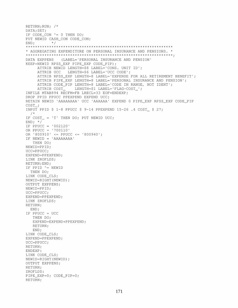
171

RETURN;RUN; /*DATA;SET;IF CODE_CON ^= 0 THEN DO;PUT NEWID CASH_CON CODE_CON;END; */**************************************************************** AGGREGATING EXPENDITURE ON PERSONAL INSURANCE AND PENSIONS. ****************************************************************;DATA EXPPENS (LABEL='PERSONAL INSURANCE AND PENSION'KEEP=NEWID RPSS_EXP PIPE_EXP CODE_PIP); ATTRIB NEWID LENGTH=$8 LABEL='CONS. UNIT ID'; ATTRIB UCC LENGTH=$6 LABEL='UCC CODE'; ATTRIB RPSS_EXP LENGTH=8 LABEL='EXPENSE FOR ALL RETIREMENT BENEFIT'; ATTRIB PIPE_EXP LENGTH=8 LABEL='PERSONAL INSURANCE AND PENSION'; ATTRIB CODE_PIP LENGTH=8 LABEL='CODE IN RANGE, NOT IDENT'; ATTRIB COST_ LENGTH=$1 LABEL='FLAG-COST_';INFILE MTAB894 RECFM=FB LRECL=33 EOF=ENDEXP;DROP PPID PPUCC PPEXPEND EXPEND UCC;RETAIN NEWID 'AAAAAAAA' UCC 'AAAAAA' EXPEND 0 PIPE_EXP RPSS_EXP CODE_PIPCOST_;INPUT PPID $ 1-8 PPUCC $ 9-14 PPEXPEND 15-26 .4 COST_ $ 27; /*IF COST_ = 'T' THEN DO; PUT NEWID UCC;END; */IF PPUCC = '002120'OR PPUCC = '700110'OR '800910' <= PPUCC <= '800940';IF NEWID = 'AAAAAAAA' THEN DO;NEWID=PPID;UCC=PPUCC;EXPEND=PPEXPEND;LINK ZROFLDS;RETURN;END;IF PPID ^= NEWID THEN DO;LINK CODE_CLS;NEWID=RIGHT(NEWID);OUTPUT EXPPENS;NEWID=PPID;UCC=PPUCC;EXPEND=PPEXPEND;LINK ZROFLDS;RETURN; END;IF PPUCC = UCC THEN DO; EXPEND=EXPEND+PPEXPEND; RETURN; END;LINK CODE_CLS;EXPEND=PPEXPEND;UCC=PPUCC;RETURN;ENDEXP:LINK CODE_CLS;NEWID=RIGHT(NEWID);OUTPUT EXPPENS;RETURN;ZROFLDS:PIPE_EXP=0; CODE_PIP=0;RETURN;

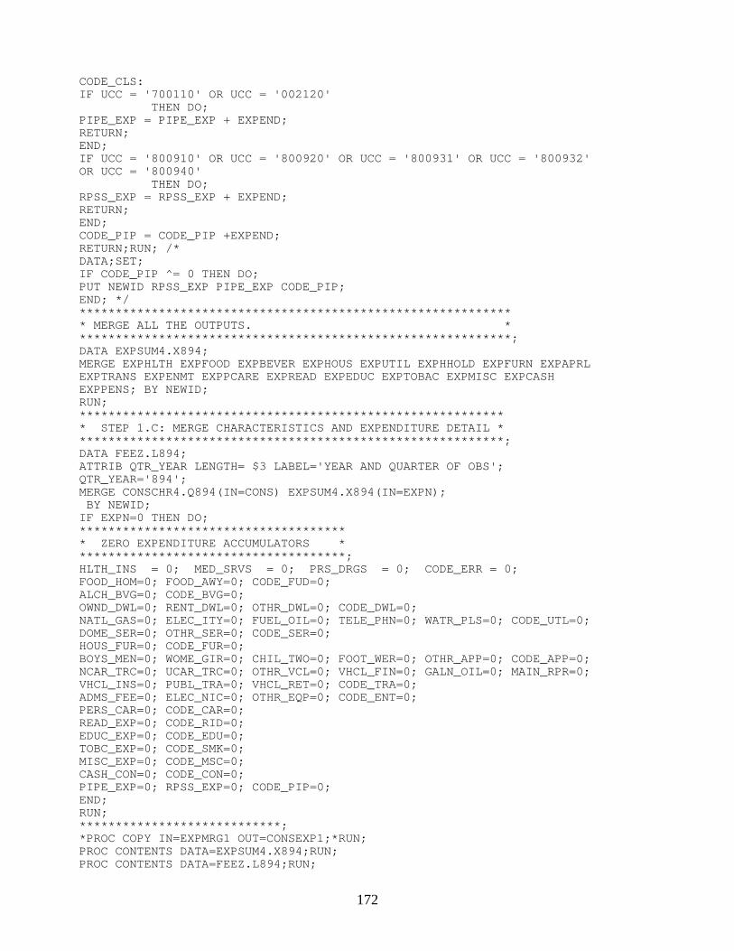
172

CODE_CLS:IF UCC = '700110' OR UCC = '002120' THEN DO;PIPE_EXP = PIPE_EXP + EXPEND;RETURN;END;IF UCC = '800910' OR UCC = '800920' OR UCC = '800931' OR UCC = '800932'OR UCC = '800940' THEN DO;RPSS_EXP = RPSS_EXP + EXPEND;RETURN;END;CODE_PIP = CODE_PIP +EXPEND;RETURN;RUN; /*DATA;SET;IF CODE_PIP ^= 0 THEN DO;PUT NEWID RPSS_EXP PIPE_EXP CODE_PIP;END; */************************************************************* MERGE ALL THE OUTPUTS. *************************************************************;DATA EXPSUM4.X894;MERGE EXPHLTH EXPFOOD EXPBEVER EXPHOUS EXPUTIL EXPHHOLD EXPFURN EXPAPRLEXPTRANS EXPENMT EXPPCARE EXPREAD EXPEDUC EXPTOBAC EXPMISC EXPCASHEXPPENS; BY NEWID;RUN;************************************************************ STEP 1.C: MERGE CHARACTERISTICS AND EXPENDITURE DETAIL ************************************************************;DATA FEEZ.L894;ATTRIB QTR_YEAR LENGTH= $3 LABEL='YEAR AND QUARTER OF OBS';QTR_YEAR='894';MERGE CONSCHR4.Q894(IN=CONS) EXPSUM4.X894(IN=EXPN); BY NEWID;IF EXPN=0 THEN DO;************************************** ZERO EXPENDITURE ACCUMULATORS **************************************;HLTH_INS = 0; MED_SRVS = 0; PRS_DRGS = 0; CODE_ERR = 0;FOOD_HOM=0; FOOD_AWY=0; CODE_FUD=0;ALCH_BVG=0; CODE_BVG=0;OWND_DWL=0; RENT_DWL=0; OTHR_DWL=0; CODE_DWL=0;NATL_GAS=0; ELEC_ITY=0; FUEL_OIL=0; TELE_PHN=0; WATR_PLS=0; CODE_UTL=0;DOME_SER=0; OTHR_SER=0; CODE_SER=0;HOUS_FUR=0; CODE_FUR=0;BOYS_MEN=0; WOME_GIR=0; CHIL_TWO=0; FOOT_WER=0; OTHR_APP=0; CODE_APP=0;NCAR_TRC=0; UCAR_TRC=0; OTHR_VCL=0; VHCL_FIN=0; GALN_OIL=0; MAIN_RPR=0;VHCL_INS=0; PUBL_TRA=0; VHCL_RET=0; CODE_TRA=0;ADMS_FEE=0; ELEC_NIC=0; OTHR_EQP=0; CODE_ENT=0;PERS_CAR=0; CODE_CAR=0;READ_EXP=0; CODE_RID=0;EDUC_EXP=0; CODE_EDU=0;TOBC_EXP=0; CODE_SMK=0;MISC_EXP=0; CODE_MSC=0;CASH_CON=0; CODE_CON=0;PIPE_EXP=0; RPSS_EXP=0; CODE_PIP=0;END;RUN;****************************;*PROC COPY IN=EXPMRG1 OUT=CONSEXP1;*RUN;PROC CONTENTS DATA=EXPSUM4.X894;RUN;PROC CONTENTS DATA=FEEZ.L894;RUN;

173

/*//* EXEC PGM=IEFBR14//*CONSCHR4 DD DSN=UN.BERHSAM.CONSCHR4,UNIT=DISK,//* DISP=(OLD,DELETE)//*EXPSUM4 DD DSN=UN.BERHSAM.EXPSUM4,UNIT=DISK,//* DISP=(OLD,DELETE)

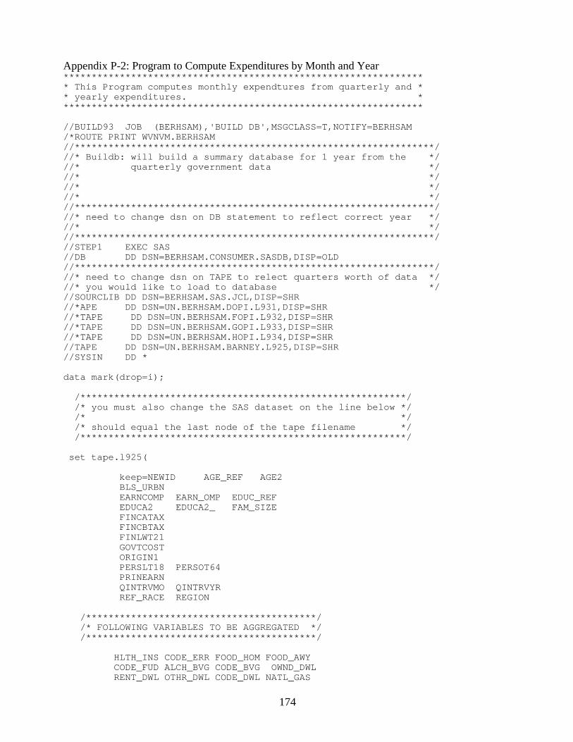
174

Appendix P-2: Program to Compute Expenditures by Month and Year***************************************************************** This Program computes monthly expendtures from quarterly and ** yearly expenditures. *****************************************************************

//BUILD93 JOB (BERHSAM),'BUILD DB',MSGCLASS=T,NOTIFY=BERHSAM /*ROUTE PRINT WVNVM.BERHSAM //****************************************************************/ //* Buildb: will build a summary database for 1 year from the */ //* quarterly government data */ //* */ //* */ //* */ //****************************************************************/ //* need to change dsn on DB statement to reflect correct year */ //* */ //****************************************************************/ //STEP1 EXEC SAS //DB DD DSN=BERHSAM.CONSUMER.SASDB,DISP=OLD //****************************************************************/ //* need to change dsn on TAPE to relect quarters worth of data */ //* you would like to load to database */ //SOURCLIB DD DSN=BERHSAM.SAS.JCL,DISP=SHR //*APE DD DSN=UN.BERHSAM.DOPI.L931,DISP=SHR //*TAPE DD DSN=UN.BERHSAM.FOPI.L932,DISP=SHR //*TAPE DD DSN=UN.BERHSAM.GOPI.L933,DISP=SHR //*TAPE DD DSN=UN.BERHSAM.HOPI.L934,DISP=SHR //TAPE DD DSN=UN.BERHSAM.BARNEY.L925,DISP=SHR //SYSIN DD * data mark(drop=i); /**********************************************************/ /* you must also change the SAS dataset on the line below */ /* */ /* should equal the last node of the tape filename */ /**********************************************************/ set tape.l925( keep=NEWID AGE_REF AGE2 BLS_URBN EARNCOMP EARN_OMP EDUC_REF EDUCA2 EDUCA2_ FAM_SIZE FINCATAX FINCBTAX FINLWT21 GOVTCOST ORIGIN1 PERSLT18 PERSOT64 PRINEARN QINTRVMO QINTRVYR REF_RACE REGION /*****************************************/ /* FOLLOWING VARIABLES TO BE AGGREGATED */ /*****************************************/ HLTH_INS CODE_ERR FOOD_HOM FOOD_AWY CODE_FUD ALCH_BVG CODE_BVG OWND_DWL RENT_DWL OTHR_DWL CODE_DWL NATL_GAS

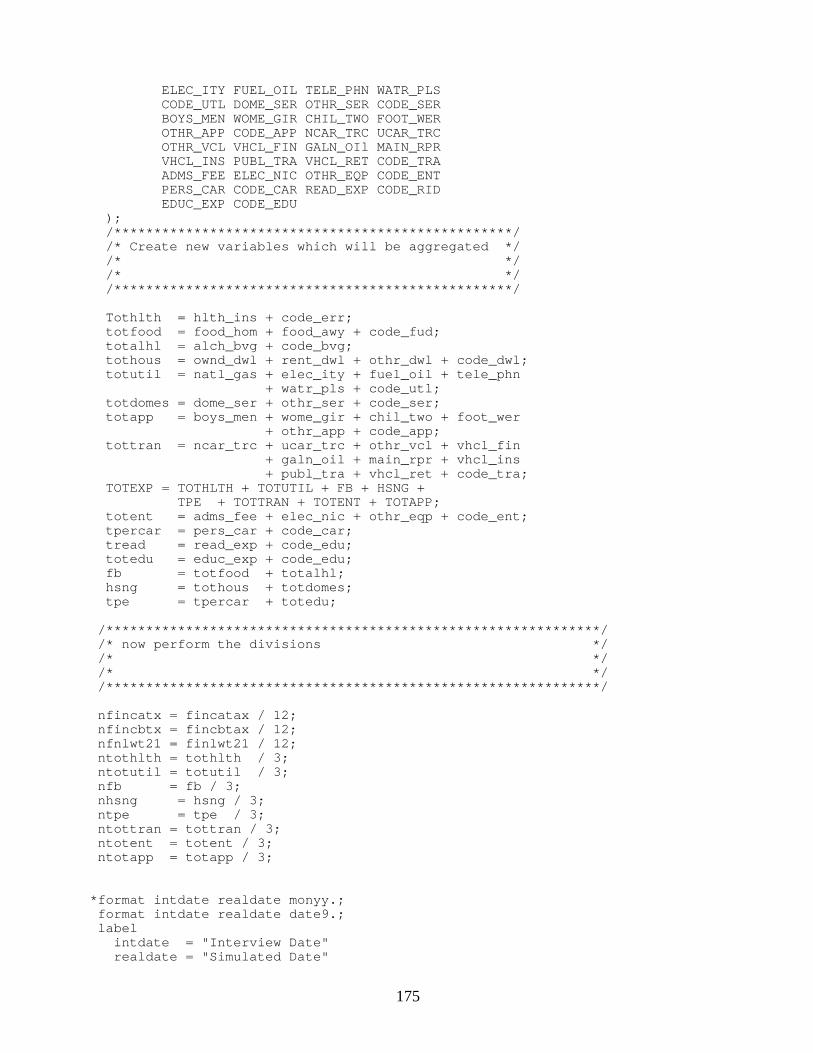
175

ELEC_ITY FUEL_OIL TELE_PHN WATR_PLS CODE_UTL DOME_SER OTHR_SER CODE_SER BOYS_MEN WOME_GIR CHIL_TWO FOOT_WER OTHR_APP CODE_APP NCAR_TRC UCAR_TRC OTHR_VCL VHCL_FIN GALN_OIl MAIN_RPR VHCL_INS PUBL_TRA VHCL_RET CODE_TRA ADMS_FEE ELEC_NIC OTHR_EQP CODE_ENT PERS_CAR CODE_CAR READ_EXP CODE_RID EDUC_EXP CODE_EDU ); /**************************************************/ /* Create new variables which will be aggregated */ /* */ /* */ /**************************************************/ Tothlth = hlth_ins + code_err; totfood = food_hom + food_awy + code_fud; totalhl = alch_bvg + code_bvg; tothous = ownd_dwl + rent_dwl + othr_dwl + code_dwl; totutil = natl_gas + elec_ity + fuel_oil + tele_phn + watr_pls + code_utl; totdomes = dome_ser + othr_ser + code_ser; totapp = boys_men + wome_gir + chil_two + foot_wer + othr_app + code_app; tottran = ncar_trc + ucar_trc + othr_vcl + vhcl_fin + galn_oil + main_rpr + vhcl_ins + publ_tra + vhcl_ret + code_tra; TOTEXP = TOTHLTH + TOTUTIL + FB + HSNG + TPE + TOTTRAN + TOTENT + TOTAPP; totent = adms_fee + elec_nic + othr_eqp + code_ent; tpercar = pers_car + code_car; tread = read_exp + code_edu; totedu = educ_exp + code_edu; fb = totfood + totalhl; hsng = tothous + totdomes; tpe = tpercar + totedu; /**************************************************************/ /* now perform the divisions */ /* */ /* */ /**************************************************************/ nfincatx = fincatax / 12; nfincbtx = fincbtax / 12; nfnlwt21 = finlwt21 / 12; ntothlth = tothlth / 3; ntotutil = totutil / 3; nfb = fb / 3; nhsng = hsng / 3; ntpe = tpe / 3; ntottran = tottran / 3; ntotent = totent / 3; ntotapp = totapp / 3; *format intdate realdate monyy.; format intdate realdate date9.; label intdate = "Interview Date" realdate = "Simulated Date"

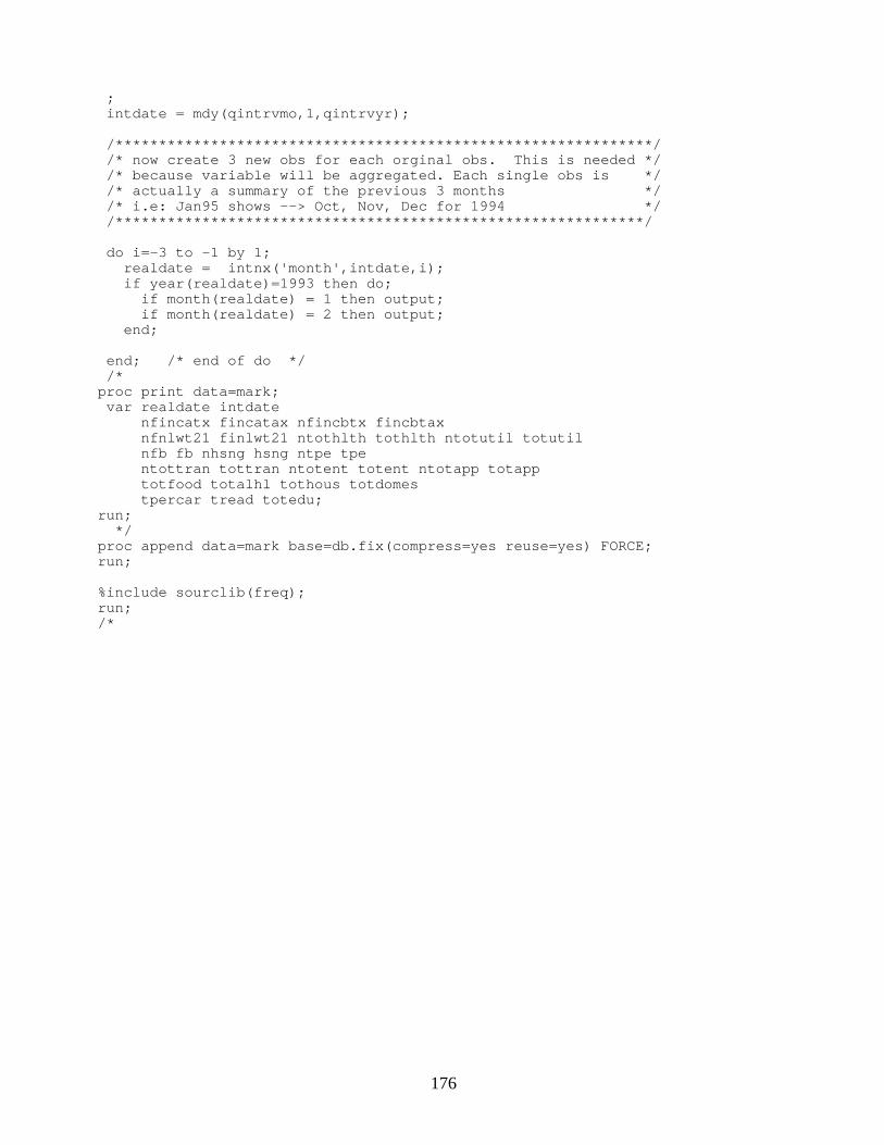
176

; intdate = mdy(qintrvmo,1,qintrvyr); /**************************************************************/ /* now create 3 new obs for each orginal obs. This is needed */ /* because variable will be aggregated. Each single obs is */ /* actually a summary of the previous 3 months */ /* i.e: Jan95 shows --> Oct, Nov, Dec for 1994 */ /*************************************************************/ do i=-3 to -1 by 1; realdate = intnx('month',intdate,i); if year(realdate)=1993 then do; if month(realdate) = 1 then output; if month(realdate) = 2 then output; end; end; /* end of do */ /* proc print data=mark; var realdate intdate nfincatx fincatax nfincbtx fincbtax nfnlwt21 finlwt21 ntothlth tothlth ntotutil totutil nfb fb nhsng hsng ntpe tpe ntottran tottran ntotent totent ntotapp totapp totfood totalhl tothous totdomes tpercar tread totedu; run; */ proc append data=mark base=db.fix(compress=yes reuse=yes) FORCE; run; %include sourclib(freq); run; /*

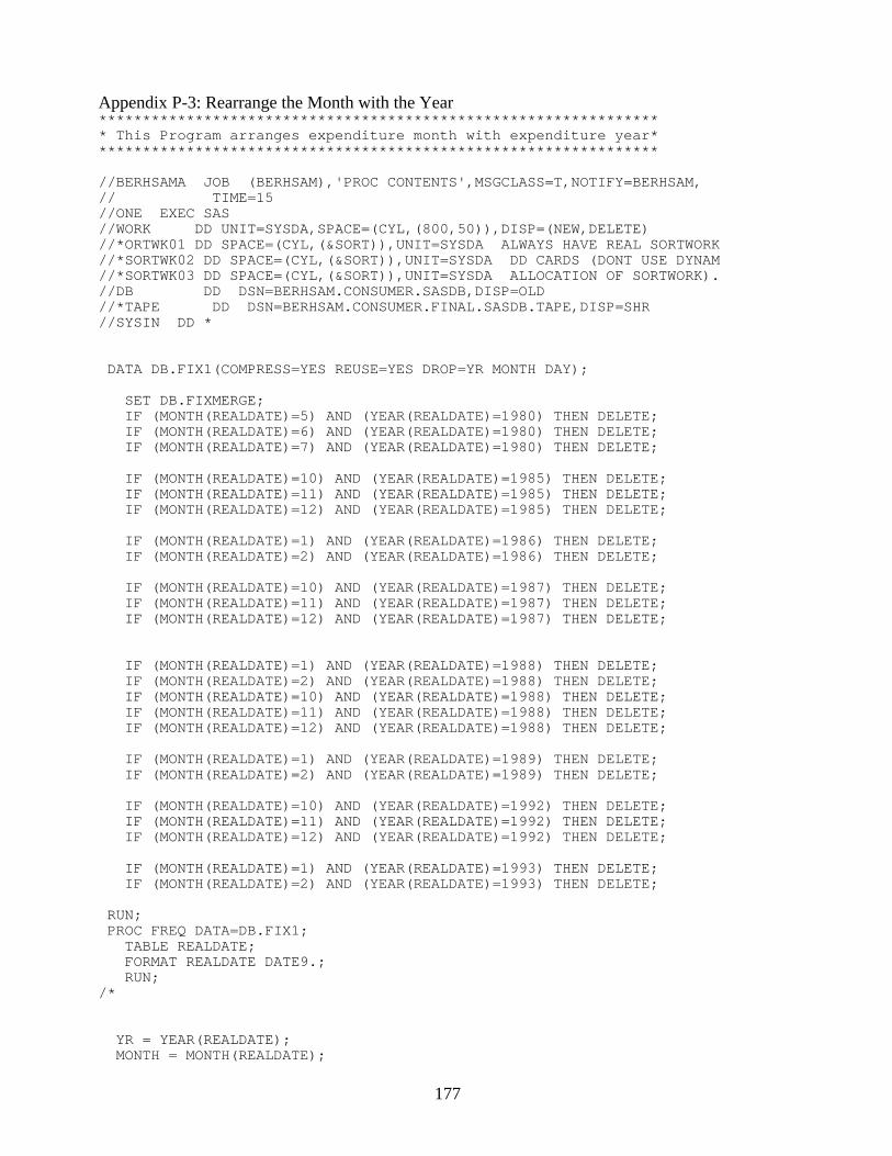
177

Appendix P-3: Rearrange the Month with the Year ***************************************************************** This Program arranges expenditure month with expenditure year*****************************************************************

//BERHSAMA JOB (BERHSAM),'PROC CONTENTS',MSGCLASS=T,NOTIFY=BERHSAM, // TIME=15 //ONE EXEC SAS //WORK DD UNIT=SYSDA,SPACE=(CYL,(800,50)),DISP=(NEW,DELETE) //*ORTWK01 DD SPACE=(CYL,(&SORT)),UNIT=SYSDA ALWAYS HAVE REAL SORTWORK //*SORTWK02 DD SPACE=(CYL,(&SORT)),UNIT=SYSDA DD CARDS (DONT USE DYNAM //*SORTWK03 DD SPACE=(CYL,(&SORT)),UNIT=SYSDA ALLOCATION OF SORTWORK). //DB DD DSN=BERHSAM.CONSUMER.SASDB,DISP=OLD //*TAPE DD DSN=BERHSAM.CONSUMER.FINAL.SASDB.TAPE,DISP=SHR //SYSIN DD * DATA DB.FIX1(COMPRESS=YES REUSE=YES DROP=YR MONTH DAY); SET DB.FIXMERGE; IF (MONTH(REALDATE)=5) AND (YEAR(REALDATE)=1980) THEN DELETE; IF (MONTH(REALDATE)=6) AND (YEAR(REALDATE)=1980) THEN DELETE; IF (MONTH(REALDATE)=7) AND (YEAR(REALDATE)=1980) THEN DELETE; IF (MONTH(REALDATE)=10) AND (YEAR(REALDATE)=1985) THEN DELETE; IF (MONTH(REALDATE)=11) AND (YEAR(REALDATE)=1985) THEN DELETE; IF (MONTH(REALDATE)=12) AND (YEAR(REALDATE)=1985) THEN DELETE; IF (MONTH(REALDATE)=1) AND (YEAR(REALDATE)=1986) THEN DELETE; IF (MONTH(REALDATE)=2) AND (YEAR(REALDATE)=1986) THEN DELETE; IF (MONTH(REALDATE)=10) AND (YEAR(REALDATE)=1987) THEN DELETE; IF (MONTH(REALDATE)=11) AND (YEAR(REALDATE)=1987) THEN DELETE; IF (MONTH(REALDATE)=12) AND (YEAR(REALDATE)=1987) THEN DELETE; IF (MONTH(REALDATE)=1) AND (YEAR(REALDATE)=1988) THEN DELETE; IF (MONTH(REALDATE)=2) AND (YEAR(REALDATE)=1988) THEN DELETE; IF (MONTH(REALDATE)=10) AND (YEAR(REALDATE)=1988) THEN DELETE; IF (MONTH(REALDATE)=11) AND (YEAR(REALDATE)=1988) THEN DELETE; IF (MONTH(REALDATE)=12) AND (YEAR(REALDATE)=1988) THEN DELETE; IF (MONTH(REALDATE)=1) AND (YEAR(REALDATE)=1989) THEN DELETE; IF (MONTH(REALDATE)=2) AND (YEAR(REALDATE)=1989) THEN DELETE; IF (MONTH(REALDATE)=10) AND (YEAR(REALDATE)=1992) THEN DELETE; IF (MONTH(REALDATE)=11) AND (YEAR(REALDATE)=1992) THEN DELETE; IF (MONTH(REALDATE)=12) AND (YEAR(REALDATE)=1992) THEN DELETE; IF (MONTH(REALDATE)=1) AND (YEAR(REALDATE)=1993) THEN DELETE; IF (MONTH(REALDATE)=2) AND (YEAR(REALDATE)=1993) THEN DELETE; RUN; PROC FREQ DATA=DB.FIX1; TABLE REALDATE; FORMAT REALDATE DATE9.; RUN; /* YR = YEAR(REALDATE); MONTH = MONTH(REALDATE);

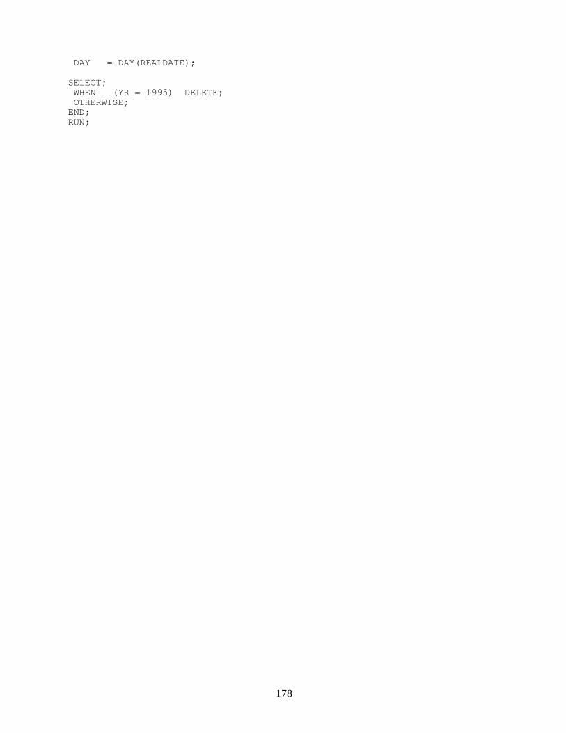
178

DAY = DAY(REALDATE); SELECT; WHEN (YR = 1995) DELETE; OTHERWISE; END; RUN;

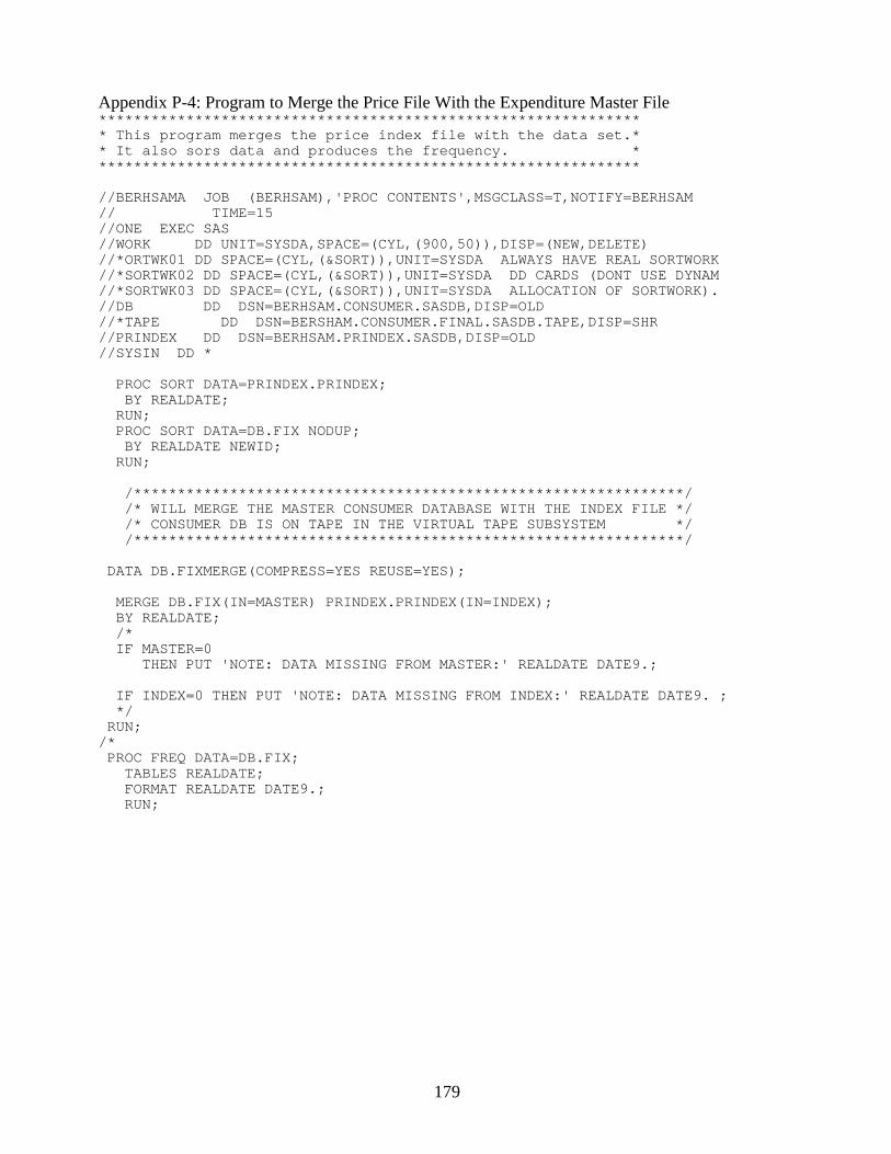
179

Appendix P-4: Program to Merge the Price File With the Expenditure Master File*************************************************************** This program merges the price index file with the data set.** It also sors data and produces the frequency. ***************************************************************

//BERHSAMA JOB (BERHSAM),'PROC CONTENTS',MSGCLASS=T,NOTIFY=BERHSAM // TIME=15 //ONE EXEC SAS //WORK DD UNIT=SYSDA,SPACE=(CYL,(900,50)),DISP=(NEW,DELETE) //*ORTWK01 DD SPACE=(CYL,(&SORT)),UNIT=SYSDA ALWAYS HAVE REAL SORTWORK //*SORTWK02 DD SPACE=(CYL,(&SORT)),UNIT=SYSDA DD CARDS (DONT USE DYNAM //*SORTWK03 DD SPACE=(CYL,(&SORT)),UNIT=SYSDA ALLOCATION OF SORTWORK). //DB DD DSN=BERHSAM.CONSUMER.SASDB,DISP=OLD //*TAPE DD DSN=BERSHAM.CONSUMER.FINAL.SASDB.TAPE,DISP=SHR //PRINDEX DD DSN=BERHSAM.PRINDEX.SASDB,DISP=OLD //SYSIN DD * PROC SORT DATA=PRINDEX.PRINDEX; BY REALDATE; RUN; PROC SORT DATA=DB.FIX NODUP; BY REALDATE NEWID; RUN; /***************************************************************/ /* WILL MERGE THE MASTER CONSUMER DATABASE WITH THE INDEX FILE */ /* CONSUMER DB IS ON TAPE IN THE VIRTUAL TAPE SUBSYSTEM */ /***************************************************************/ DATA DB.FIXMERGE(COMPRESS=YES REUSE=YES); MERGE DB.FIX(IN=MASTER) PRINDEX.PRINDEX(IN=INDEX); BY REALDATE; /* IF MASTER=0 THEN PUT 'NOTE: DATA MISSING FROM MASTER:' REALDATE DATE9.; IF INDEX=0 THEN PUT 'NOTE: DATA MISSING FROM INDEX:' REALDATE DATE9. ; */ RUN; /* PROC FREQ DATA=DB.FIX; TABLES REALDATE; FORMAT REALDATE DATE9.; RUN;

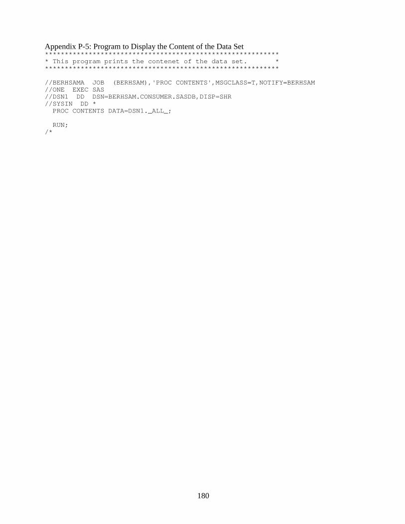
180

Appendix P-5: Program to Display the Content of the Data Set************************************************************ This program prints the contenet of the data set. ************************************************************

//BERHSAMA JOB (BERHSAM),'PROC CONTENTS',MSGCLASS=T,NOTIFY=BERHSAM //ONE EXEC SAS //DSN1 DD DSN=BERHSAM.CONSUMER.SASDB,DISP=SHR //SYSIN DD * PROC CONTENTS DATA=DSN1._ALL_; RUN; /*

181

Appendix P-6: Program to Copy File******************************************************* This program is used to copy a file to another file*******************************************************

//BERHSAMA JOB (BERHSAM),'PROC CONTENTS',MSGCLASS=T,NOTIFY=BERHSAM, // TIME=1440 //* WILL COPY DISK CONSUMER DATABASE TO TAPE //* //ONE EXEC SAS //*WORK DD UNIT=SYSDA,SPACE=(CYL,(500,50)),DISP=(NEW,DELETE) //*ORTWK01 DD SPACE=(CYL,(&SORT)),UNIT=SYSDA ALWAYS HAVE REAL SORTWORK //*SORTWK02 DD SPACE=(CYL,(&SORT)),UNIT=SYSDA DD CARDS (DONT USE DYNAM //*SORTWK03 DD SPACE=(CYL,(&SORT)),UNIT=SYSDA ALLOCATION OF SORTWORK) //TAPE DD DSN=BERHSAM.CONSUMER.SURVEY.NOV0197,DISP=(NEW,CATLG), // UNIT=VTS //DB DD DSN=BERHSAM.CONSUMER.SASDB,DISP=SHR //SYSIN DD * PROC COPY IN=DB OUT=TAPE; RUN; ENDSAS; RUN;

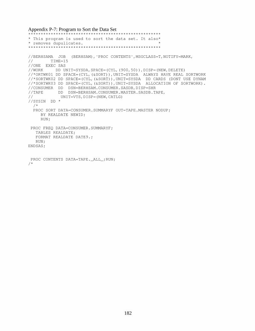
182

Appendix P-7: Program to Sort the Data Set****************************************************** This program is used to sort the data set. It also** removes dupulicates. ******************************************************

//BERHSAMA JOB (BERHSAM),'PROC CONTENTS',MSGCLASS=T,NOTIFY=MARK, // TIME=15 //ONE EXEC SAS //WORK DD UNIT=SYSDA,SPACE=(CYL,(900,50)),DISP=(NEW,DELETE) //*ORTWK01 DD SPACE=(CYL,(&SORT)),UNIT=SYSDA ALWAYS HAVE REAL SORTWORK //*SORTWK02 DD SPACE=(CYL,(&SORT)),UNIT=SYSDA DD CARDS (DONT USE DYNAM //*SORTWK03 DD SPACE=(CYL,(&SORT)),UNIT=SYSDA ALLOCATION OF SORTWORK). //CONSUMER DD DSN=BERHSAM.CONSUMER.SASDB,DISP=SHR //TAPE DD DSN=BERHSAM.CONSUMER.MASTER.SASDB.TAPE, // UNIT=VTS,DISP=(NEW,CATLG) //SYSIN DD * /* PROC SORT DATA=CONSUMER.SUMMARYF OUT=TAPE.MASTER NODUP; BY REALDATE NEWID; RUN; PROC FREQ DATA=CONSUMER.SUMMARYF; TABLES REALDATE; FORMAT REALDATE DATE9.; RUN; ENDSAS; PROC CONTENTS DATA=TAPE._ALL_;RUN; /*

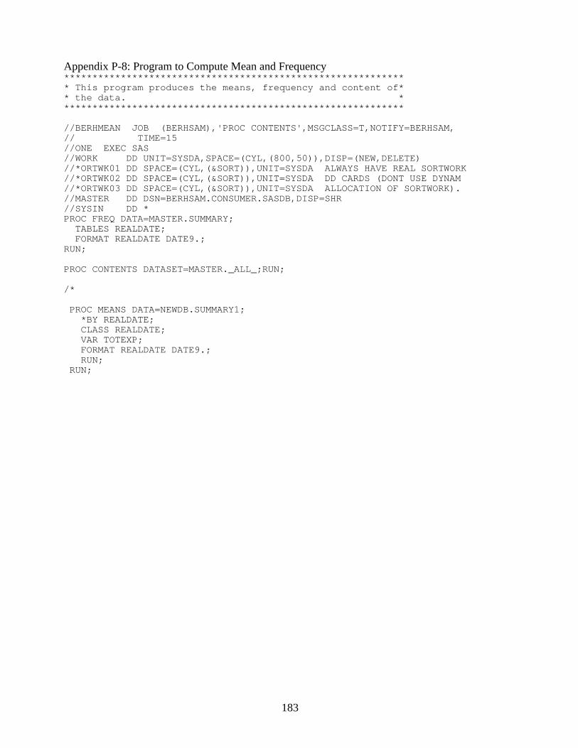
183

Appendix P-8: Program to Compute Mean and Frequency ************************************************************* This program produces the means, frequency and content of** the data. *************************************************************

//BERHMEAN JOB (BERHSAM),'PROC CONTENTS',MSGCLASS=T,NOTIFY=BERHSAM, // TIME=15 //ONE EXEC SAS //WORK DD UNIT=SYSDA,SPACE=(CYL,(800,50)),DISP=(NEW,DELETE) //*ORTWK01 DD SPACE=(CYL,(&SORT)),UNIT=SYSDA ALWAYS HAVE REAL SORTWORK //*ORTWK02 DD SPACE=(CYL,(&SORT)),UNIT=SYSDA DD CARDS (DONT USE DYNAM //*ORTWK03 DD SPACE=(CYL,(&SORT)),UNIT=SYSDA ALLOCATION OF SORTWORK). //MASTER DD DSN=BERHSAM.CONSUMER.SASDB,DISP=SHR //SYSIN DD * PROC FREQ DATA=MASTER.SUMMARY; TABLES REALDATE; FORMAT REALDATE DATE9.; RUN; PROC CONTENTS DATASET=MASTER._ALL_;RUN; /* PROC MEANS DATA=NEWDB.SUMMARY1; *BY REALDATE; CLASS REALDATE; VAR TOTEXP; FORMAT REALDATE DATE9.; RUN; RUN;

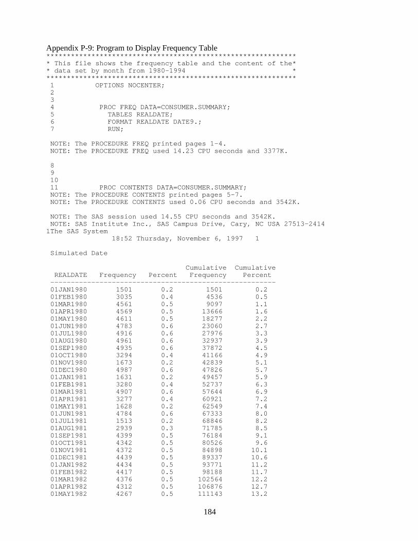
184

Appendix P-9: Program to Display Frequency Table************************************************************** This file shows the frequency table and the content of the** data set by month from 1980-1994 ************************************************************** 1 OPTIONS NOCENTER; 2 3 4 PROC FREQ DATA=CONSUMER.SUMMARY; 5 TABLES REALDATE; 6 FORMAT REALDATE DATE9.; 7 RUN; NOTE: The PROCEDURE FREQ printed pages 1-4. NOTE: The PROCEDURE FREQ used 14.23 CPU seconds and 3377K. 8 9 10 11 PROC CONTENTS DATA=CONSUMER.SUMMARY; NOTE: The PROCEDURE CONTENTS printed pages 5-7. NOTE: The PROCEDURE CONTENTS used 0.06 CPU seconds and 3542K. NOTE: The SAS session used 14.55 CPU seconds and 3542K. NOTE: SAS Institute Inc., SAS Campus Drive, Cary, NC USA 27513-24141The SAS System 18:52 Thursday, November 6, 1997 1 Simulated Date Cumulative Cumulative REALDATE Frequency Percent Frequency Percent ------------------------------------------------------- 01JAN1980 1501 0.2 1501 0.2 01FEB1980 3035 0.4 4536 0.5 01MAR1980 4561 0.5 9097 1.1 01APR1980 4569 0.5 13666 1.6 01MAY1980 4611 0.5 18277 2.2 01JUN1980 4783 0.6 23060 2.7 01JUL1980 4916 0.6 27976 3.3 01AUG1980 4961 0.6 32937 3.9 01SEP1980 4935 0.6 37872 4.5 01OCT1980 3294 0.4 41166 4.9 01NOV1980 1673 0.2 42839 5.1 01DEC1980 4987 0.6 47826 5.7 01JAN1981 1631 0.2 49457 5.9 01FEB1981 3280 0.4 52737 6.3 01MAR1981 4907 0.6 57644 6.9 01APR1981 3277 0.4 60921 7.2 01MAY1981 1628 0.2 62549 7.4 01JUN1981 4784 0.6 67333 8.0 01JUL1981 1513 0.2 68846 8.2 01AUG1981 2939 0.3 71785 8.5 01SEP1981 4399 0.5 76184 9.1 01OCT1981 4342 0.5 80526 9.6 01NOV1981 4372 0.5 84898 10.1 01DEC1981 4439 0.5 89337 10.6 01JAN1982 4434 0.5 93771 11.2 01FEB1982 4417 0.5 98188 11.7 01MAR1982 4376 0.5 102564 12.2 01APR1982 4312 0.5 106876 12.7 01MAY1982 4267 0.5 111143 13.2

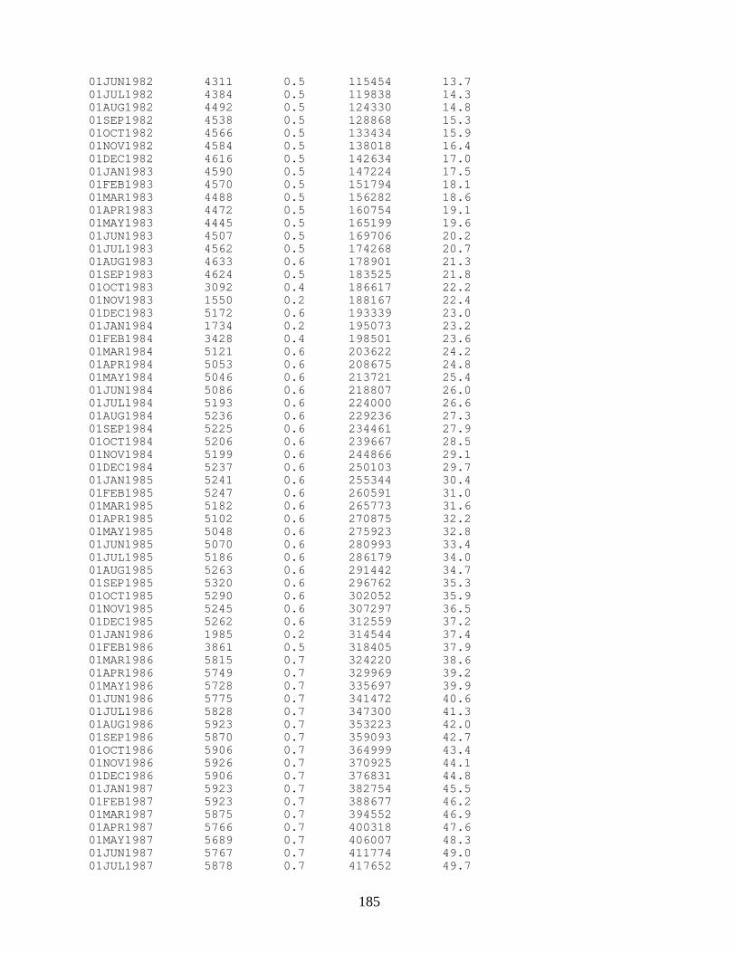
185

01JUN1982 4311 0.5 115454 13.7 01JUL1982 4384 0.5 119838 14.3 01AUG1982 4492 0.5 124330 14.8 01SEP1982 4538 0.5 128868 15.3 01OCT1982 4566 0.5 133434 15.9 01NOV1982 4584 0.5 138018 16.4 01DEC1982 4616 0.5 142634 17.0 01JAN1983 4590 0.5 147224 17.5 01FEB1983 4570 0.5 151794 18.1 01MAR1983 4488 0.5 156282 18.6 01APR1983 4472 0.5 160754 19.1 01MAY1983 4445 0.5 165199 19.6 01JUN1983 4507 0.5 169706 20.2 01JUL1983 4562 0.5 174268 20.7 01AUG1983 4633 0.6 178901 21.3 01SEP1983 4624 0.5 183525 21.8 01OCT1983 3092 0.4 186617 22.2 01NOV1983 1550 0.2 188167 22.4 01DEC1983 5172 0.6 193339 23.0 01JAN1984 1734 0.2 195073 23.2 01FEB1984 3428 0.4 198501 23.6 01MAR1984 5121 0.6 203622 24.2 01APR1984 5053 0.6 208675 24.8 01MAY1984 5046 0.6 213721 25.4 01JUN1984 5086 0.6 218807 26.0 01JUL1984 5193 0.6 224000 26.6 01AUG1984 5236 0.6 229236 27.3 01SEP1984 5225 0.6 234461 27.9 01OCT1984 5206 0.6 239667 28.5 01NOV1984 5199 0.6 244866 29.1 01DEC1984 5237 0.6 250103 29.7 01JAN1985 5241 0.6 255344 30.4 01FEB1985 5247 0.6 260591 31.0 01MAR1985 5182 0.6 265773 31.6 01APR1985 5102 0.6 270875 32.2 01MAY1985 5048 0.6 275923 32.8 01JUN1985 5070 0.6 280993 33.4 01JUL1985 5186 0.6 286179 34.0 01AUG1985 5263 0.6 291442 34.7 01SEP1985 5320 0.6 296762 35.3 01OCT1985 5290 0.6 302052 35.9 01NOV1985 5245 0.6 307297 36.5 01DEC1985 5262 0.6 312559 37.2 01JAN1986 1985 0.2 314544 37.4 01FEB1986 3861 0.5 318405 37.9 01MAR1986 5815 0.7 324220 38.6 01APR1986 5749 0.7 329969 39.2 01MAY1986 5728 0.7 335697 39.9 01JUN1986 5775 0.7 341472 40.6 01JUL1986 5828 0.7 347300 41.3 01AUG1986 5923 0.7 353223 42.0 01SEP1986 5870 0.7 359093 42.7 01OCT1986 5906 0.7 364999 43.4 01NOV1986 5926 0.7 370925 44.1 01DEC1986 5906 0.7 376831 44.8 01JAN1987 5923 0.7 382754 45.5 01FEB1987 5923 0.7 388677 46.2 01MAR1987 5875 0.7 394552 46.9 01APR1987 5766 0.7 400318 47.6 01MAY1987 5689 0.7 406007 48.3 01JUN1987 5767 0.7 411774 49.0 01JUL1987 5878 0.7 417652 49.7

186

01AUG1987 5954 0.7 423606 50.4 01SEP1987 5999 0.7 429605 51.1 01OCT1987 1785 0.2 431390 51.3 01NOV1987 3552 0.4 434942 51.7 01DEC1987 5286 0.6 440228 52.3 01JAN1988 1670 0.2 441898 52.5 01FEB1988 3301 0.4 445199 52.9 01MAR1988 4994 0.6 450193 53.5 01APR1988 4958 0.6 455151 54.1 01MAY1988 4975 0.6 460126 54.7 01JUN1988 5040 0.6 465166 55.3 01JUL1988 5119 0.6 470285 55.9 01AUG1988 5198 0.6 475483 56.5 01SEP1988 5190 0.6 480673 57.2 01OCT1988 3476 0.4 484149 57.6 01NOV1988 1749 0.2 485898 57.8 01DEC1988 5153 0.6 491051 58.4 01JAN1989 1688 0.2 492739 58.6 01FEB1989 3422 0.4 496161 59.0 01MAR1989 5076 0.6 501237 59.6 01APR1989 5078 0.6 506315 60.2 01MAY1989 4987 0.6 511302 60.8 01JUN1989 5008 0.6 516310 61.4 01JUL1989 5028 0.6 521338 62.0 01AUG1989 5100 0.6 526438 62.6 01SEP1989 5104 0.6 531542 63.2 01OCT1989 5088 0.6 536630 63.8 01NOV1989 5085 0.6 541715 64.4 01DEC1989 5139 0.6 546854 65.0 01JAN1990 5201 0.6 552055 65.6 01FEB1990 5206 0.6 557261 66.3 01MAR1990 5169 0.6 562430 66.9 01APR1990 5106 0.6 567536 67.5 01MAY1990 5023 0.6 572559 68.1 01JUN1990 5045 0.6 577604 68.7 01JUL1990 5120 0.6 582724 69.3 01AUG1990 5184 0.6 587908 69.9 01SEP1990 5168 0.6 593076 70.5 01OCT1990 5190 0.6 598266 71.1 01NOV1990 5161 0.6 603427 71.8 01DEC1990 5188 0.6 608615 72.4 01JAN1991 3398 0.4 612013 72.8 01FEB1991 1729 0.2 613742 73.0 01MAR1991 5091 0.6 618833 73.6 01APR1991 1678 0.2 620511 73.8 01MAY1991 3299 0.4 623810 74.2 01JUN1991 5066 0.6 628876 74.8 01JUL1991 5126 0.6 634002 75.4 01AUG1991 5205 0.6 639207 76.0 01SEP1991 5181 0.6 644388 76.6 01OCT1991 5151 0.6 649539 77.2 01NOV1991 5171 0.6 654710 77.9 01DEC1991 5158 0.6 659868 78.5 01JAN1992 5203 0.6 665071 79.1 01FEB1992 5232 0.6 670303 79.7 01MAR1992 5157 0.6 675460 80.3 01APR1992 5152 0.6 680612 80.9 01MAY1992 5094 0.6 685706 81.5 01JUN1992 5165 0.6 690871 82.2 01JUL1992 5197 0.6 696068 82.8 01AUG1992 5234 0.6 701302 83.4 01SEP1992 5223 0.6 706525 84.0

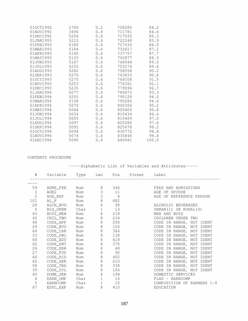
187

01OCT1992 1760 0.2 708285 84.2 01NOV1992 3496 0.4 711781 84.6 01DEC1992 5254 0.6 717035 85.3 01JAN1993 5213 0.6 722248 85.9 01FEB1993 5185 0.6 727433 86.5 01MAR1993 5184 0.6 732617 87.1 01APR1993 5140 0.6 737757 87.7 01MAY1993 5120 0.6 742877 88.3 01JUN1993 5167 0.6 748044 89.0 01JUL1993 5232 0.6 753276 89.6 01AUG1993 5282 0.6 758558 90.2 01SEP1993 5275 0.6 763833 90.8 01OCT1993 5275 0.6 769108 91.5 01NOV1993 5253 0.6 774361 92.1 01DEC1993 5235 0.6 779596 92.7 01JAN1994 5277 0.6 784873 93.3 01FEB1994 5255 0.6 790128 94.0 01MAR1994 5158 0.6 795286 94.6 01APR1994 5070 0.6 800356 95.2 01MAY1994 5044 0.6 805400 95.8 01JUN1994 5034 0.6 810434 96.4 01JUL1994 5055 0.6 815489 97.0 01AUG1994 5097 0.6 820586 97.6 01SEP1994 5092 0.6 825678 98.2 01OCT1994 5094 0.6 830772 98.8 01NOV1994 5074 0.6 835846 99.4 01DEC1994 5095 0.6 840941 100.0 CONTENTS PROCEDURE -----Alphabetic List of Variables and Attributes----- # Variable Type Len Pos Format Label ---------------------------------------------------------------------------------- 59 ADMS_FEE Num 8 346 FEES AND ADMISSIONS 3 AGE2 Num 3 11 AGE OF SPOUSE 2 AGE_REF Num 3 8 AGE OF REFERENCE PERSON 101 AL_P Num 8 682 28 ALCH_BVG Num 8 98 ALCHOLIC BEVERAGES 4 BLS_URBN Char 1 14 URBAN(1) OR RURAL(0) 43 BOYS_MEN Num 8 218 MEN AND BOYS 45 CHIL_TWO Num 8 234 CHILDREN UNDER TWO 48 CODE_APP Num 8 258 CODE IN RANGE, NOT IDENT 29 CODE_BVG Num 8 106 CODE IN RANGE, NOT IDENT 64 CODE_CAR Num 8 386 CODE IN RANGE, NOT IDENT 33 CODE_DWL Num 8 138 CODE IN RANGE, NOT IDENT 68 CODE_EDU Num 8 418 CODE IN RANGE, NOT IDENT 62 CODE_ENT Num 8 370 CODE IN RANGE, NOT IDENT 24 CODE_ERR Num 8 68 CODE IN RANGE, NOT IDENT 27 CODE_FUD Num 8 90 CODE IN RANGE, NOT IDENT 66 CODE_RID Num 8 402 CODE IN RANGE, NOT IDENT 42 CODE_SER Num 8 210 CODE IN RANGE, NOT IDENT 58 CODE_TRA Num 8 338 CODE IN RANGE, NOT IDENT 39 CODE_UTL Num 8 186 CODE IN RANGE, NOT IDENT 40 DOME_SER Num 8 194 DOMESTIC SERVICES 6 EARN_OMP Char 1 16 FLAG - EARNCOMP 5 EARNCOMP Char 1 15 COMPOSITION OF EARNERS 1-8 67 EDUC_EXP Num 8 410 EDUCATION

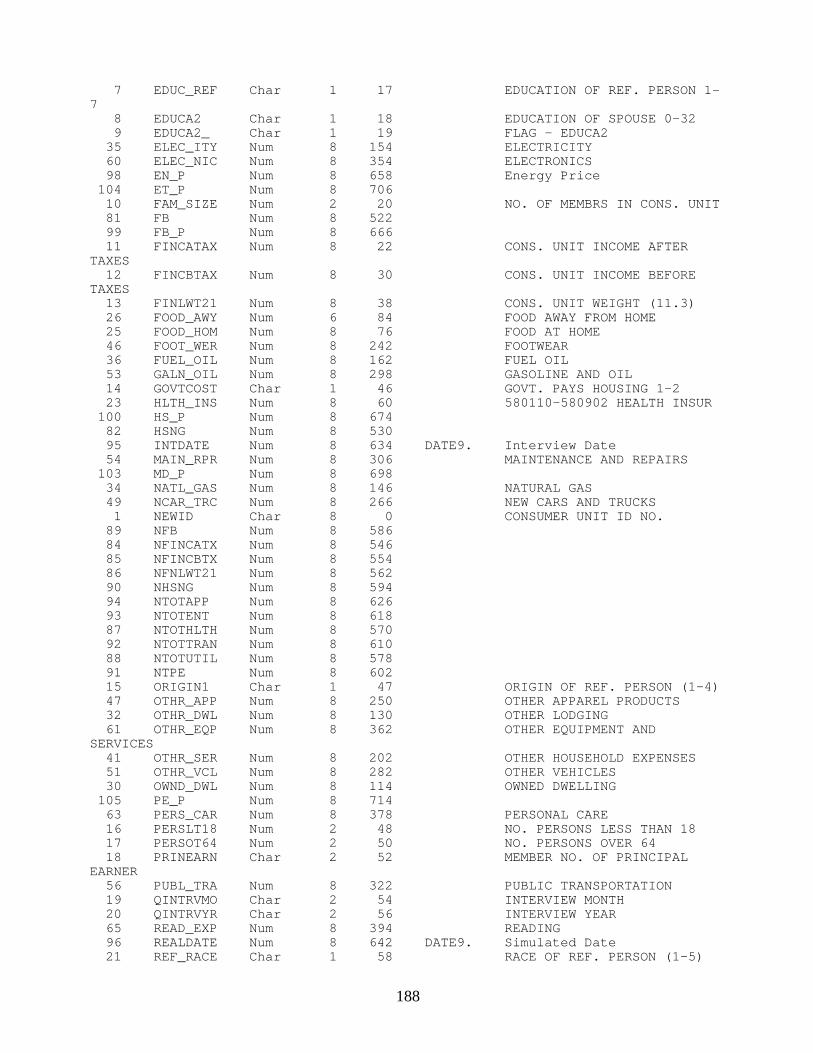
188

7 EDUC_REF Char 1 17 EDUCATION OF REF. PERSON 1-7 8 EDUCA2 Char 1 18 EDUCATION OF SPOUSE 0-32 9 EDUCA2_ Char 1 19 FLAG - EDUCA2 35 ELEC_ITY Num 8 154 ELECTRICITY 60 ELEC_NIC Num 8 354 ELECTRONICS 98 EN_P Num 8 658 Energy Price 104 ET_P Num 8 706 10 FAM_SIZE Num 2 20 NO. OF MEMBRS IN CONS. UNIT 81 FB Num 8 522 99 FB_P Num 8 666 11 FINCATAX Num 8 22 CONS. UNIT INCOME AFTERTAXES 12 FINCBTAX Num 8 30 CONS. UNIT INCOME BEFORETAXES 13 FINLWT21 Num 8 38 CONS. UNIT WEIGHT (11.3) 26 FOOD_AWY Num 6 84 FOOD AWAY FROM HOME 25 FOOD_HOM Num 8 76 FOOD AT HOME 46 FOOT_WER Num 8 242 FOOTWEAR 36 FUEL_OIL Num 8 162 FUEL OIL 53 GALN_OIL Num 8 298 GASOLINE AND OIL 14 GOVTCOST Char 1 46 GOVT. PAYS HOUSING 1-2 23 HLTH_INS Num 8 60 580110-580902 HEALTH INSUR 100 HS_P Num 8 674 82 HSNG Num 8 530 95 INTDATE Num 8 634 DATE9. Interview Date 54 MAIN_RPR Num 8 306 MAINTENANCE AND REPAIRS 103 MD_P Num 8 698 34 NATL_GAS Num 8 146 NATURAL GAS 49 NCAR_TRC Num 8 266 NEW CARS AND TRUCKS 1 NEWID Char 8 0 CONSUMER UNIT ID NO. 89 NFB Num 8 586 84 NFINCATX Num 8 546 85 NFINCBTX Num 8 554 86 NFNLWT21 Num 8 562 90 NHSNG Num 8 594 94 NTOTAPP Num 8 626 93 NTOTENT Num 8 618 87 NTOTHLTH Num 8 570 92 NTOTTRAN Num 8 610 88 NTOTUTIL Num 8 578 91 NTPE Num 8 602 15 ORIGIN1 Char 1 47 ORIGIN OF REF. PERSON (1-4) 47 OTHR_APP Num 8 250 OTHER APPAREL PRODUCTS 32 OTHR_DWL Num 8 130 OTHER LODGING 61 OTHR_EQP Num 8 362 OTHER EQUIPMENT ANDSERVICES 41 OTHR_SER Num 8 202 OTHER HOUSEHOLD EXPENSES 51 OTHR_VCL Num 8 282 OTHER VEHICLES 30 OWND_DWL Num 8 114 OWNED DWELLING 105 PE_P Num 8 714 63 PERS_CAR Num 8 378 PERSONAL CARE 16 PERSLT18 Num 2 48 NO. PERSONS LESS THAN 18 17 PERSOT64 Num 2 50 NO. PERSONS OVER 64 18 PRINEARN Char 2 52 MEMBER NO. OF PRINCIPALEARNER 56 PUBL_TRA Num 8 322 PUBLIC TRANSPORTATION 19 QINTRVMO Char 2 54 INTERVIEW MONTH 20 QINTRVYR Char 2 56 INTERVIEW YEAR 65 READ_EXP Num 8 394 READING 96 REALDATE Num 8 642 DATE9. Simulated Date 21 REF_RACE Char 1 58 RACE OF REF. PERSON (1-5)

189

22 REGION Char 1 59 CENSUS REGION(URBAN ONLY)(1-4) 31 RENT_DWL Num 8 122 RENTED DWELLING 37 TELE_PHN Num 8 170 TELEPHONE 71 TOTALHL Num 8 442 75 TOTAPP Num 8 474 74 TOTDOMES Num 8 466 80 TOTEDU Num 8 514 77 TOTENT Num 8 490 97 TOTEXP Num 8 650 70 TOTFOOD Num 8 434 69 TOTHLTH Num 8 426 72 TOTHOUS Num 8 450 76 TOTTRAN Num 8 482 73 TOTUTIL Num 8 458 83 TPE Num 8 538 78 TPERCAR Num 8 498 102 TR_P Num 8 690 79 TREAD Num 8 506 50 UCAR_TRC Num 8 274 USED CARS AND TRUCKS 52 VHCL_FIN Num 8 290 VEHICLE FINANCE CHARGES 55 VHCL_INS Num 8 314 VEHICLE INSURANCE 57 VHCL_RET Num 8 330 VEHICLE RENTAL 38 WATR_PLS Num 8 178 WATER AND OTHER SERVICES 44 WOME_GIR Num 8 226 WOMEN AND GIRLS -----Sort Information----- Sortedby: REALDATE NEWID Validated: YES Character Set: EBCDIC Sort Option: NODUPKEY