The all-weather portfolio - NTNU Open

NTN

UN

orw

egia

n U

nive

rsity

of S

cien

ce a

nd T

echn

olog

yFa

culty

of E

cono

mic

s an

d M

anag

emen

t N

TNU

Bus

ines

s Sc

hool

Lars Andreas Forsmo SimonsenMarkus Hermo

The all-weather portfolio

A review of Bridgewater Associates investmentstrategy: The all-weather portfolio

Master’s thesis in Economics and Business AdministrationSupervisor: Denis M. Becker

May 2021

Mas

ter’s

thes

is




Master’s thesis in Economics and Business AdministrationSupervisor: Denis M. BeckerMay 2021

Norwegian University of Science and TechnologyFaculty of Economics and ManagementNTNU Business School

i

Preface

The master thesis is written as a part of NTNU Handelshøyskolens master program in

Economics and Business Administration. This is a master thesis in the field of Finance and

Investment spring 2021. The thesis examines one of Bridgewater’s investing strategies and

the choice of theme is due to the authors’ common interest in finance and investment

strategies.

The process has been both time demanding and challenging, but also instructive and

educational. We would like to thank our supervisor Denis M. Becker for all the help and

constructive feedback along the way.

The authors take full responsibility for the content of this thesis. NTNU does not have any

responsibility for the content or views in the thesis.

Norwegian University of Science and Technology

May, 2021

---------------------------------------------------- ----------------------------------------------------

Lars Andreas Forsmo Simonsen Markus Hermo

ii

Abstract

The objective of this thesis is to investigate the relevance of the all-weather portfolio, created

by Bridgewater Associates, and compare it with two traditional portfolios: 60/40 and all-

equity. In addition, the assumptions made by Bridgewater Associates regarding the all-

weather portfolio is examined. Using quarterly data from 1970 to 2021, we explore how the

portfolios perform in terms of historical returns and different risk- and drawdowns

measurements. Furthermore, we tested whether asset classes have biases to perform better in

different economic states using average return and OLS regression. We further calculated the

historical Sharpe ratio to test Bridgewater’s assumptions that all assets have a similar risk-

adjusted return. We find that the all-weather portfolio provides a higher risk-adjusted return

than the 60/40 and all-equity portfolios, and that it has a lower downside risk for the sample

period. However, we cannot confirm that the assumptions in Bridgewater Associates theory

are valid. The relationship between asset classes with inflation and economic growth showed

rather inconsistent results. Further, the assumption of similar risk-adjusted return for the asset

classes were also rejected as the results exhibited a large difference in Sharpe ratio.

Altogether, the results obtained from this thesis indicate that the portfolio has a higher risk-

adjusted return and lower downside risk for our sample period. However, we cannot confirm

that this is because of the relationships proposed by Bridgewater Associates.

iii

Table of content

Preface i

Abstract ii

Table of content iii

List of tables v

List of figures vi

1 Introduction 1

2 Literature review 3

2.1 Theoretical framework 3

2.1.1 Factor models 3

2.1.2 Modern portfolio theory 5

2.1.3 Risk factor parity 6

2.2 The Bridgewater philosophy 9

2.2.1 All-weather portfolio explained 9

2.2.2 A review of Bridgewater’s economic market approach 11

2.2.3 Volatility of asset classes 13

2.2.4 Asset biases towards economic environments 14

2.2.4.1 Equities 14

2.2.4.2 U.S. Treasuries 15

2.2.4.3 Commodities 15

2.2.4.4 Gold 16

3 Data and methodology 18

3.1 Data 18

3.2 Calculation of asset class returns 19

3.3 Dependent variables 21

3.4 Independent variables 22

3.5 Construction and backtesting of the all-weather portfolio 24

3.5.1 Construction of the all-weather portfolio 24

3.5.2 Historical return and different risk- and drawdown measures 26

3.6 Testing for asset class bias 29

3.6.1 Average return tests 29

3.6.2 Ordinary least squares regression 30

3.6.3 Testing of ordinary least square assumptions 31

iv

3.7 Historical risk-adjusted returns for the different asset classes 33

4 Empirical results and discussion 34

4.1 Results from construction and backtesting of the all-weather portfolio 34

4.1.1 Weights in all-weather portfolio 34

4.1.2 Historical return and different risk- and drawdown measures 36

4.1.2.1 Historical return and risk measures 36

4.1.2.2 Drawdown measures 40

4.2 Results from the economic bias tests 42

4.2.1 Results from average return tests 42

4.2.2 Results from regression analysis 44

4.3 Results from the risk-adjusted return test 46

5 Conclusion and further prospects 47

6 References 50

Appendices 54

Appendix A: Descriptive statistics 54

Appendix B: OLS assumptions 55

Appendix C: Robustness test for average return tests 62

Appendix D: Historical Sharpe Ratio in five different decades 64

v

List of tables

Table 3.1 - Asset class bias and preferred economic states...................................................... 24

Table 3.2 - Definition of the four sub-portfolios ...................................................................... 25

Table 3.3 - Description of the four economic biases ................................................................ 29

Table 3.4 - Description of the four economic states ................................................................ 29

Table 4.1 - Weights in asset classes ......................................................................................... 34

Table 4.2 - Weights in sub-portfolios ....................................................................................... 34

Table 4.3 - Risk balance between economic states .................................................................. 35

Table 4.4 - Risk balance between economic biases ................................................................. 35

Table 4.5 - Historical statistics ................................................................................................. 36

Table 4.6 - Statistics for rolling holding periods ...................................................................... 37

Table 4.7 - Average excess return in periods of either high or low inflation/GDP growth ..... 38

Table 4.8 - Average excess return in the four economic states ................................................ 39

Table 4.9 - Drawdown statistical measures .............................................................................. 41

Table 4.10 - Average excess return in periods of either high or low inflation/GDP growth ... 42

Table 4.11 - Average excess return in the four economic states .............................................. 43

Table 4.12 - Regression analysis for asset class bias ............................................................... 44

Table 4.13 - Risk-adjusted return test ...................................................................................... 46

vi

List of figures

Figure 2.1 - Capital and risk allocation in 60/40 ........................................................................ 7

Figure 2.2 - Capital and risk allocation in 25/75 ........................................................................ 7

Figure 2.3 - The three key drivers of the economy .................................................................. 11

Figure 3.1 - The four economic states ...................................................................................... 24

Figure 4.1 - Historical return for the full sample period .......................................................... 36

Figure 4.2 - Drawdowns for the all-weather portfolio ............................................................. 40

Figure 4.3 - Drawdowns for the 60/40 portfolio ...................................................................... 40

Figure 4.4 - Drawdowns for the all-equity portfolio ................................................................ 40

1

1 Introduction

Since the early 1980 the yield on US treasuries have been steadily falling until March 2020

when the 10-year US treasury bond hit an all-time low at 0.54% (U.S. Department of the

Treasury, 2021). Ever-falling interest rates are bad news for investors in general and this has

led many to increase the share of equities in their portfolio to achieve a higher expected

return. The traditional portfolio allocation strategy where one invests 60 percent in equities

and 40 percent in government bonds may not give a satisfactory return as the general yields

are expected to remain low for the foreseeable future (Blanchard, 2019). Some advisors are

now suggesting that a long-term investor should invest all their money into equity because of

its higher expected return (Lian et al., 2019).

However, history has shown that investing all your money in equity is a very risky approach

as the stock market has a tendency to become highly correlated and have big declines during

economic turmoil (Bruder & Roncalli, 2012). In addition to being highly volatile during

economic turmoil’s, the stock market also tends to go into longer periods with low and even

negative returns. Being equity heavy is unfortunately the conventional method that the world's

pension funds have taken, and this leads to a high concentration in equity risk (Prince, 2011).

Bridgewater’s founder Ray Dalio proposes the all-weather portfolio as the solution for the

age-old problem of how to best allocate capital. The goal of this type of investment strategy is

to perform well in all economic environments, thereby minimizing the downside without

giving up too much of the expected return. Dalio (2004) has stated that the portfolio has

approximately the same level of return as the stock market, but a significantly lower downside

risk, making it an investment that is superior to the 60/40 and all-equity portfolios.

The primary objective of this thesis is to analyse whether a portfolio constructed on the basis

of the all-weather portfolio principles would have a low downside risk and still yield a

satisfying return. In addition, we investigate the assumptions made by Dalio and Bridgewater

regarding the all-weather portfolio. First, that there is a timeless and reliable relationship

between asset classes and macroeconomic risk factors, such as inflation and economic

growth. Second, that all asset classes have approximately the same risk-adjusted return. To

limit the size of the task, we have chosen to use macro-economic data from the United States,

since the U.S. economy is the largest and most influential.

2

The following research question has been formulated for this research:

How does the all-weather portfolio perform compared to the 60/40 and all-equity portfolios,

and are the assumptions for the all-weather portfolio valid?

This research question is further tested by the following three hypotheses.

Null hypothesis 1: The all-weather portfolio does not have a higher risk-adjusted return and

lower downside risk than the 60/40 and all-equity portfolios.

Null hypothesis 2: Asset classes do not have a tendency to perform better in the preferred

economic state as defined in Table 3.1.

Null hypothesis 3: The different asset classes do not have similar risk-adjusted excess return.

The first hypothesis is a test of the historical performance of the all-weather portfolio, and the

second and third hypothesis is a test of the most important assumptions that Bridgewater

Associates makes regarding the all-weather portfolio.

The rest of this thesis is structured as follows. Chapter 2 reviews the financial theory

regarding factor models and modern portfolio theory. The risk parity approach is also

examined to identify whether it can solve some of the problems with modern portfolio theory.

Furthermore, Bridgewater’s philosophy is reviewed with the focus on the assumptions on

which the all-weather portfolio is based. Chapter 3 presents the dataset and examines how the

returns and the dependent and independent variables are calculated. The methodology for the

construction of the all-weather portfolio, backtesting, testing asset class bias, and testing risk-

adjusted return are also presented in this chapter. Chapter 4 presents and discusses the results

of the three tests conducted. Chapter 5 summarizes the results and concludes the thesis.

3

2 Literature review

This chapter summarizes theoretical statements and empirical findings from previous research

literature on factor models, modern portfolio theory and risk parity. Moreover, different

literature is reviewed to examine the potential and credibility of the all-weather portfolio.

2.1 Theoretical framework

2.1.1 Factor models

Risk factor models are an approach where one uses the underlying risk factors and their risk

premium as a means to explain the risk premiums on asset classes. Factor models generally

decompose the return on assets into two types of components; the first type is correlated

across assets and is often referred to as the underlying risk factors. These are believed to have

an effect on all assets, but to a varying degree (Ang, 2014). The second type is asset specific

and is therefore not correlated across assets.

The first factor model is the capital asset pricing model (CAPM) used by Sharpe (1964),

Lintner (1965), and Mossin (1966). The CAPM takes only the market risk factor into account

and is therefore most applicable for equities. The sensitivity towards the market risk factor is

often referred to as the market beta, and the size of this beta reflects how much the assets

change, on average, when the overall stock market changes by 1%. The market beta is a

measure of the inherent risk in the equity market as a whole. This is often referred to as the

systematic risk, and it cannot be diversified away.

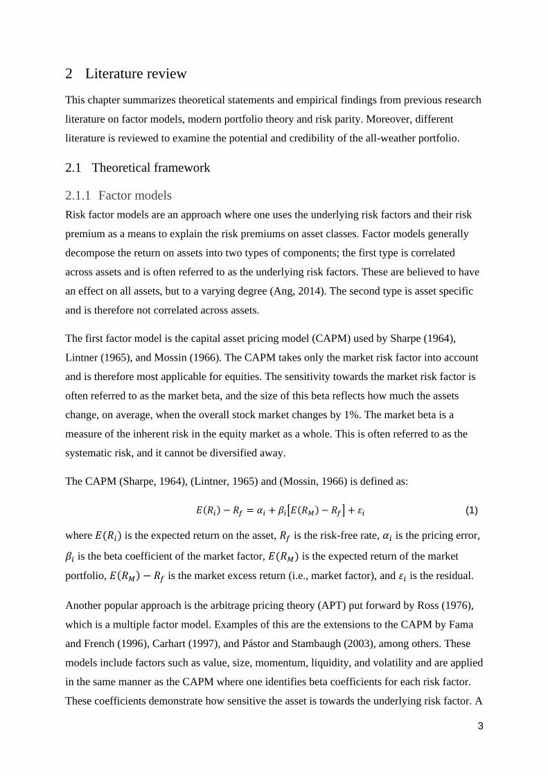
The CAPM (Sharpe, 1964), (Lintner, 1965) and (Mossin, 1966) is defined as:

𝐸(𝑅𝑖) − 𝑅𝑓 = 𝛼𝑖 + 𝛽𝑖[𝐸(𝑅𝑀) − 𝑅𝑓] + 𝜀𝑖 (1)

where 𝐸(𝑅𝑖) is the expected return on the asset, 𝑅𝑓 is the risk-free rate, 𝛼𝑖 is the pricing error,

𝛽𝑖 is the beta coefficient of the market factor, 𝐸(𝑅𝑀) is the expected return of the market

portfolio, 𝐸(𝑅𝑀) − 𝑅𝑓 is the market excess return (i.e., market factor), and 𝜀𝑖 is the residual.

Another popular approach is the arbitrage pricing theory (APT) put forward by Ross (1976),

which is a multiple factor model. Examples of this are the extensions to the CAPM by Fama

and French (1996), Carhart (1997), and Pástor and Stambaugh (2003), among others. These

models include factors such as value, size, momentum, liquidity, and volatility and are applied

in the same manner as the CAPM where one identifies beta coefficients for each risk factor.

These coefficients demonstrate how sensitive the asset is towards the underlying risk factor. A

4

key feature of both the CAPM and the APT is that there is a linear relation between asset risk

premium and the risk premium associated with one or several risk factors (Barucci & Fontana,

2017).

The APT (Ross, 1976) is defined as:

𝐸(𝑅𝑖) − 𝑅𝑓 = 𝛼𝑖 + 𝛽𝑖′𝑓 + 𝜀𝑖 (2)

where 𝐸(𝑅𝑖) is the expected return on asset 𝑖, 𝑅𝑓 is the risk-free rate, 𝛼𝑖 is the pricing error,

𝛽𝑖′ is the vector of factor loadings, 𝑓 is the risk factors, and 𝜀𝑖 is the residual.

Leite et al., (2020) examined whether the risk factors of the Fama-French five-factor model

could be proxies for macro risk factors. They found that when aggregate dividend yield, term

spread, default spread, one-month T-bill and consumer price index (CPI) are included; high

minus low (HML), small minus big (SMB), and robust minus weak (RMW) lose their

explanatory ability. This indicates that macro variables may be the real underlying risk

factors.

Risk factors can generally be categorized into three types: investment, dynamic, and macro

factors (Ang, 2014). In this thesis, the focus is on macro factors because they are more

universal for all asset classes, which is in line with the view of Bridgewater Associates – see

Chapter 2.2.

The application of risk factor models means that all asset returns can be explained by a linear

combination of risk factors, risk premiums (beta coefficient), and a random component (the

residual) that is often referred to as an unsystematic risk component or idiosyncratic risk

component. The idiosyncratic risk component is bigger for single securities, such as a single

stock, and this component gets smaller as the number of securities in the portfolio increases

(Mokkelbost, 1971). This implies that an allocation to whole asset classes will reduce the

importance of idiosyncratic risk, and thereby increase the importance of systematic risk

factors.

5

2.1.2 Modern portfolio theory

Modern portfolio theory (MPT) – also known as the mean-variance model – was first put

forward by Markowitz (1952). In his article ‘Portfolio Selection’ he describes a framework in

which an optimizing investor is looking to maximize the return for a given level of risk. The

main idea is that if one has several assets that are less than perfectly correlated one could

obtain a higher expected return for a given level of risk by combining the assets. The author

assumed that the world is uncertain, and that each investment has a probability distribution of

potential outcomes, where one can only estimate the expected return and expected risk level

(variance or volatility). Since it is not known which asset class will have the highest rate of

return, the rational investor will diversify across multiple assets (Markowitz, 1991).

According to Markowitz (1991), investors have different levels of risk aversion. This implies

that investors may obtain the same amount of utility from portfolios with different risk levels.

This is because as long as the portfolio is placed on the efficient frontier, no other portfolio

will give investors the same amount of return, without increasing the risk of the portfolio

(Markowitz, 1991). Thus, investors with different levels of preferred risk have different

optimal portfolios.

Markowitz (1991) further states that for risk averse investors the optimal portfolio is the

tangency portfolio. This is the portfolio in which all the unsystematic risk is diversified away,

leaving only systematic risk. Furthermore, given that the equity market is in equilibrium, the

market weight index would be the tangent portfolio. For a portfolio consisting of different

asset classes, the optimal portfolio would not be as easy to identify. However, one will find

the optimal portfolio by maximizing the Sharpe ratio.

The Sharpe ratio is one of the most common measurements of risk-adjusted return (Sharpe,

1994). By dividing the expected asset class return above the risk-free rate with the standard

deviation of the asset one obtains the Sharpe ratio – see Chapter 3.7 for more details.

𝑆ℎ𝑎𝑟𝑝𝑒 𝑟𝑎𝑡𝑖𝑜 =𝑅𝐴 − 𝑅𝑓

𝜎𝐴 (3)

The Markowitz (1952) mean-variance model is a simple and intuitive approach to portfolio

optimization. However, it has some major drawbacks. The optimal portfolio depends on the

expectations of returns, standard deviations, and the correlation between the different asset

classes, and it is therefore highly sensitive to errors and changes in the input parameters.

6

Destabilization of the correlation between assets and identifying which assets have the highest

expected return over time are examples of problems with the input parameters. The 2007–

2009 subprime crisis demonstrated that the mean-variance approach is not a truly effective

diversification method, as correlations tend to increase during economic crises (Bruder &

Roncalli, 2012).

Therefore, since the subprime crisis, the asset management industry has become increasingly

focused on risk management. One of the solutions developed is to allocate based on risk

instead of the market value of the different assets.

2.1.3 Risk factor parity

In contrast to MPT, risk parity focuses on the allocation of risk, thus equally weighting the

amount of risk that each part of the portfolio contributes to the total portfolio (Martellini &

Tarelli, 2015). The goal is to balance risk to gain the optimal level of return at a preferred risk

level, and to avoid long periods of poor performance. This approach bears a strong

resemblance to the ideas behind the all-weather portfolio, and Bridgewater Associates even

claim that their strategy is ‘the foundation of the risk parity movement’ (Bridgewater

Associates, 2012, p.1).

There are many definitions of risk, and variance or volatility have traditionally been used as

the standard measurement of risk. Alternative proxies for the risk of an asset class are value at

risk, conditional value at risk, and the market beta value (Szegö, 2002). According to Shahidi

(2014), it is important to factor in the volatility of the asset class in the asset allocation

process. This is because highly volatile asset classes tend to fluctuate more around average

return than less volatile asset classes. Thus, less volatile asset classes will have a lower impact

on the portfolio over time, in terms of how they affect the return. However, by allocating a

larger amount to the less volatile assets, one can ensure that the impact of fluctuations in the

various assets in the portfolio is approximately the same; thereby ensuring that the portfolio’s

return is approximately the same in all states of the economy.

Qian (2011) studied how the risk of the different components in a traditional 60/40 portfolio

contributed to the portfolio's overall risk. He found that because equities were more volatile

than bonds, the risk contribution of equities was 92% – see Figure 2.1.

7

Figure 2.1 - Capital and risk allocation in 60/40

Figure 2.2 - Capital and risk allocation in 25/75

Furthermore, Qian (2011) tested a portfolio consisting of 25% equities and 75% bonds to

balance the risk contribution of the two assets. The capital- and risk allocation of the two

portfolios are illustrated in Figure 2.1 and Figure 2.2. The author also calculated the

correlation between the two portfolios and their underlying assets. There was a 98%

correlation between the 60/40 portfolio and equities, and a 13% correlation between the 60/40

portfolio and bonds. For the 25/75 portfolio, the correlation with equities and bonds was 77%

and 77%, respectively. This is a good illustration of how one can adjust the risk contribution

of the various components in a portfolio by changing the capital allocated to its parts.

The same technique can be applied in risk factor parity. As mentioned in Chapter 2.1.1, it is

believed that movements in asset classes are determined by underlying factors. The risk factor

parity approach addresses this assumption by identifying these risk factors and subsequently

changing the allocation based on the exposure to the underlying risk factors (Bhansali, 2011).

In this way, for example, one can change the allocation so that the portfolio has a neutral

position to the underlying risk factors.

8

Page and Taborsky (2011) emphasize that economic conditions frequently undergo regime

shifts, which are documented through market turbulence, inflation, and gross domestic

product (GDP) growth. They further state that asset class returns are driven by risk factors

that are highly regime specific, which is why portfolio construction should be based on risk

factors (Page & Taborsky, 2011).

As mentioned earlier, studies have demonstrated that the correlation between asset classes

does not exhibit a stable relationship, because asset classes tend to be highly correlated in

economic turmoil (Amato & Lohre, 2020). Thus, in line with the approach of Bridgewater

Associates, this paper is focused on the correlation between asset classes and their risk factors

(i.e., inflation and economic growth), as this seems like a more stable and predictable

relationship (Bridgewater Associates, 2012).

On the other hand, ignoring the covariance between asset classes may lead to the portfolio

being highly sensitive to the particular asset classes that are included in the portfolio

(Bhansali et al., 2012). Furthermore, Baltas (2016) emphasizes that in periods of increased

asset correlation, the allocation process in which one ignores the correlation between asset

components may lead to a highly skewed risk distribution in periods. It is therefore important

to choose assets with different sensitivity towards the underlying risk factors to address the

problems with increased asset correlation.

9

2.2 The Bridgewater philosophy

2.2.1 All-weather portfolio explained

Bridgewater Associates created the all-weather investment portfolio (Bridgewater Associates,

2012). Based on their knowledge of the drivers behind economic shifts and how these shifts

affect asset class return, they developed a strategy whose goal was to adopt a neutral position

towards the different underlying risk factors (i.e., economic environments). This was to avoid

having to be dependent on successfully predicting future economic conditions (Shahidi,

2014).

According to Shahidi (2014), the underlying risk factors for asset class return can be classified

into the following three categories: (1) shift in expectations of future interest rate, (2) shift in

risk appetite, and (3) shift in the economic environment. The author further explains that the

first two categories affect all asset classes in the same manner, while the latter category is

diversifiable because there is a possibility of achieving neutral exposure to economic

environments - see Chapter 2.2.3 for more details.

Shahidi (2014) states that a neutral exposure to economic environments can be achieved by

owning assets that are going to perform above average in different economic states. Thus,

ensuring that when an unexpected shift in the economy happens, the portfolio has some assets

that are going to outperform, and hopefully give a high enough excess return to offset the loss

from the assets that are underperforming in the same state. The weighting of the different

assets in the portfolio is therefore chosen so that each economic state has the same amount of

risk, and thus ensuring that the portfolio has approximately the same expected return in each

economic state.

In Bridgewater’s article ‘The Biggest Mistake in Investing’, the author states that asset

allocation can be done by leveraging and deleveraging low/high risk assets to obtain a similar

expected return and risk for all assets in the portfolio (Jensen & Rotenberg, 2004). This

implies that all asset classes have the same risk-adjusted return (Sharpe ratio), and one can

therefore allocate based on risk only and still get the same expected return in each economic

state.

Tang and Whitelaw (2011) find evidence that the Sharpe ratio in the equity market coincides

with the phases of the business cycle over time, indicating that the Sharpe ratios in the

recession and expansion phases differ. Moreover, Tang and Whitelaw (2011) cites evidence

10

of a significantly better return/volatility tradeoff when entering expansion phases than when

leaving the expansion phase. However, Bridgewater Associates is referring to a long-term

relationship, which might be the long-term average Sharpe ratio for a longer period than the

10-year period used by Tang and Whitelaw (2011).

The founder of Bridgewater Associates, Ray Dalio, believed that ‘...all asset classes have

environmental biases’ (Bridgewater Associates, 2012, p.5). He argues, for example, that

owning a traditional equity-heavy portfolio is like taking a bet that economic growth will be

above expectations and that inflation will be below expectations. The traditional equity-heavy

portfolio is thereby exposed to a significant risk of changes regarding the economic growth

and inflation in the future.

Prince (2011) states that the price of asset classes is reflecting the expected development in

the macroeconomic variables, where inflation and economic growth are the most important.

This is because the volume of economic activity (growth) and its pricing (inflation) primarily

determines the aggregated cash flow of an asset class. The effects of whether growth and

inflation are higher or lower than what was expected will therefore influence the asset class

returns. Thus, by dividing the portfolio into four sections that perform well in different states

of the economy, one can capture the majority of risk premiums attached to owning risky

assets, but still achieve a neutral position towards the underlying risk factors.

11

2.2.2 A review of Bridgewater’s economic market approach

To gain a better understanding of the key drivers behind asset class return and why a balanced

portfolio is beneficial, one needs to understand the different factors that cause the economy to

function the way it does today (Shahidi, 2014). According to Dalio (2012), there are three

main forces that drive the economy: productivity growth, short-term debt cycle (business

cycle), and long-term debt cycle.

Figure 2.3 presents the overlays of the short-term business cycle, the long-term debt cycle,

and the productivity trend line. This figure is a simple illustration on how these three forces

affect the economy, and it serves as a useful roadmap to understand why asset price fluctuates

(Dalio, 2012).

Figure 2.3 - The three key drivers of the economy

The most important underlying driver in the economy is productivity growth. One can think

of productivity growth as the average output produced by each worker in a society (Dalio,

2012). Productivity growth per capita is the same as real per capita GDP growth, and

according to Dalio (2012), this measure has been approximately 2% per annum for the past

100 years in the US.

Figure 2.3 presents the productivity trend line, which is increasing slowly at an approximately

constant rate. This is due to the fact that we either need to improve our work ethic or learn to

work smarter for productivity to increase, and this can be a slow process. In the real world,

however, we see large fluctuations in the GDP that are caused by two types of cycles, referred

to by Dalio (2012) as the short-term and long-term debt cycles.

12

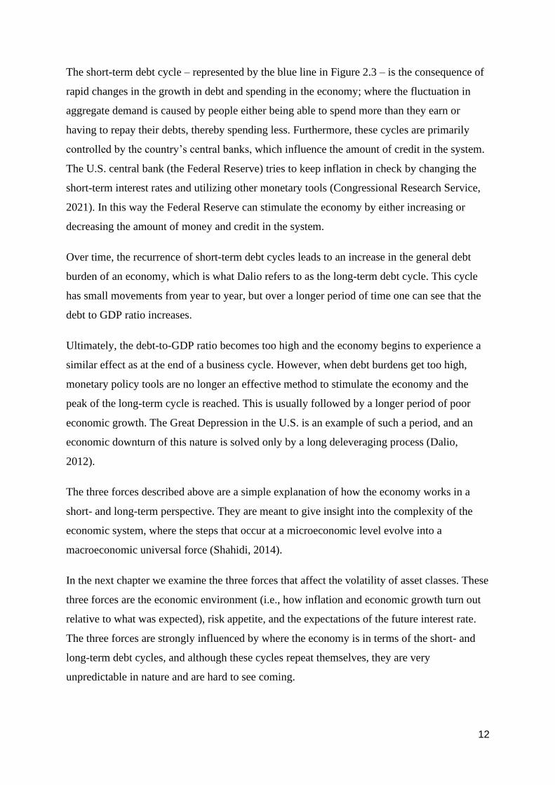
The short-term debt cycle – represented by the blue line in Figure 2.3 – is the consequence of

rapid changes in the growth in debt and spending in the economy; where the fluctuation in

aggregate demand is caused by people either being able to spend more than they earn or

having to repay their debts, thereby spending less. Furthermore, these cycles are primarily

controlled by the country’s central banks, which influence the amount of credit in the system.

The U.S. central bank (the Federal Reserve) tries to keep inflation in check by changing the

short-term interest rates and utilizing other monetary tools (Congressional Research Service,

2021). In this way the Federal Reserve can stimulate the economy by either increasing or

decreasing the amount of money and credit in the system.

Over time, the recurrence of short-term debt cycles leads to an increase in the general debt

burden of an economy, which is what Dalio refers to as the long-term debt cycle. This cycle

has small movements from year to year, but over a longer period of time one can see that the

debt to GDP ratio increases.

Ultimately, the debt-to-GDP ratio becomes too high and the economy begins to experience a

similar effect as at the end of a business cycle. However, when debt burdens get too high,

monetary policy tools are no longer an effective method to stimulate the economy and the

peak of the long-term cycle is reached. This is usually followed by a longer period of poor

economic growth. The Great Depression in the U.S. is an example of such a period, and an

economic downturn of this nature is solved only by a long deleveraging process (Dalio,

2012).

The three forces described above are a simple explanation of how the economy works in a

short- and long-term perspective. They are meant to give insight into the complexity of the

economic system, where the steps that occur at a microeconomic level evolve into a

macroeconomic universal force (Shahidi, 2014).

In the next chapter we examine the three forces that affect the volatility of asset classes. These

three forces are the economic environment (i.e., how inflation and economic growth turn out

relative to what was expected), risk appetite, and the expectations of the future interest rate.

The three forces are strongly influenced by where the economy is in terms of the short- and

long-term debt cycles, and although these cycles repeat themselves, they are very

unpredictable in nature and are hard to see coming.

13

2.2.3 Volatility of asset classes

The three factors that affect volatility in asset class return are shifts in expected interest rate,

shifts in risk appetite, and shifts in the expected economic environment.

Shifts in the expectations of future interest rates are fairly stable and the expectation of how

the interest rate will transpire over time is reflected in the treasury yield curve. However,

unanticipated changes in expected future interest rate will influence the asset class price,

which in turn will influence the asset class returns (Chen et al., 1986). Thus, the risk is

unavoidable because it will affect all asset classes.

Shifts in risk appetite is also not a diversifiable asset class risk. This is because the value of

risky assets generally moves in the same direction when there are shifts due to increasing or

decreasing risk appetite. Thus, these changes will impact all asset class prices and return

(Coudert & Gex, 2008).

The effect of both shifts in expectation of future interest rate and risk appetite can be

explained by the net present value (NPV), as shown in equation 4.

𝑁𝑒𝑡 𝑝𝑟𝑒𝑠𝑒𝑛𝑡 𝑣𝑎𝑙𝑢𝑒 𝑜𝑓 𝑎𝑠𝑠𝑒𝑡𝑛 = ∑𝐸(𝐶𝐹𝑡)

(1 + 𝑖)𝑡

𝑛

𝑡=1

(4)

The NPV is an equation used to value expected future cash flows, where the value of an asset

class will decline as the discount rate 𝑖 increases, or rise as the discount rate decreases (Greer,

1997). Ultimately, changes in expectation with regard to future interest rate and risk appetite

affect the discount rate 𝑖, but this will be the same for all asset classes and hence does not

constitute a diversifiable risk.

The expected future cash flow 𝐸(𝐶𝐹𝑡) is based on what the market expects the value of an

investment to be. If there is a shift in the expectations of the underlying factors of future cash

flow, the value of the asset class will change. Since inflation and economic growth are the

two main factors that determine the cash flow for asset classes, changes in these factors will

ultimately affect the expected future cash flow 𝐸(𝐶𝐹𝑡) (Shahidi, 2014).

Furthermore, the idea is not to diversify away the economic biases within each asset class, but

to construct a pool of different asset classes so that the portfolio will have a neutral position

towards economic biases. Shahidi (2014) emphasizes that, ‘The goal of efficient portfolio

14

construction is to capture the excess returns above cash offered by the first two parts (Shifts in

expectations of future interest rate and shift in risk appetite) and diversify away the risk of

shifts in the economic environment’ (p.46).

2.2.4 Asset biases towards economic environments

In 2011, Bridgewater Associates published a research paper, ‘Risk Parity is About Balance’,

where they stated that ‘the relationship of asset performance to growth and inflation are

reliable – indeed, timeless and universal – and knowable, rooted in the duration and sources of

variability of the assets cash flow’ (Prince, 2011, p. 4).

The choice of asset classes in the portfolio is based on their sensitivity to the underlying risk

factors. For example, the opposite sensitivity of stocks and bonds to economic growth, and the

opposite sensitivity of bonds and commodities to inflation makes the combination of these

assets risk reducing for the portfolio (Ilmanen et al., 2014). This thesis follows the all-season

portfolio in terms of which asset classes that are included in the portfolio (Robbins, 2014).

The logical relationship that economic growth- and inflation have with the different asset

classes is presented below.

2.2.4.1 Equities

According to Shahidi (2014), equities tend to outperform expected returns when economic

growth exceeds expectations. The author further argues that this is because the return on

equities is a function of two primary variables, namely revenue and profit margins; where a

positive shift in expected economic growth will ultimately lead to increased expectations in

relation to the level of revenue. This theory is shared by Ang (2014), who also explains that

equities underperform and are more volatile in periods of low economic growth.

In addition, Shahidi (2014) claims that equities tend to perform better than average when

inflation is lower than expected. This is due to the fact that businesses generally have higher

profit margins when prices of input goods (i.e., the cost of goods and services) are lower than

expected, and when the central bank cuts interest rates to avoid deflation. The reason for this

is that the savings on input and interest are not passed on to consumers, as the price on their

products is already set. On the other hand, when inflation is higher than expected, equities

tend to perform lower than average, and are therefore a poor hedge against inflation (Ang,

2014).

15

2.2.4.2 U.S. Treasuries

Shahidi (2014) states that treasuries perform better in periods when economic growth and

inflation are lower than expected. This is because of the high probability that the central bank

will act and lower interest rates.

U.S. Treasuries are considered a risk-free asset in the sense that they have no call, event, or

default risk, and they have virtually no liquidity risk. They are fixed income securities, which

means that if one buys a 20-year treasury bond, one receives the same coupon payment twice

a year. At the issue date, the yield-to-maturity is approximately the same as the coupon rate.

Thus, if the prevailing interest rate in the market is lower than the coupon rate, then the value

is higher than the face value (Finra, 2021). Since bonds have a fixed interest rate, a decline in

the interest rate in the market is beneficial for treasuries (Shahidi, 2014). However, the return

calculation is more complicated when holding a bond portfolio with constant time to maturity,

which is the case for the all-weather portfolio – see Chapter 3.2.

In addition to the mathematical function in relation to changes in interest rate, treasuries are

also well-recognized as a safe haven and are therefore an attractive asset class in periods of

low economic growth. The fact that they act as a hedge in periods of turmoil and uncertainty

makes treasuries a highly recommended option to balance the portfolio (Gupta et al., 2021).

2.2.4.3 Commodities

According to Shahidi (2014), commodities are biased to have better-than-average returns

when economic growth is higher than expected. This is because the price of commodities is

determined by supply and demand. If the economy is performing better than expected by the

producers of commodities (i.e., leading to higher unexpected demand for commodities), there

might be a shortage of supply, which would drive up prices. Research by Ang (2014) also

found that returns on commodities are higher when economic growth is high, especially for

energy and agriculture. This also means that commodities tend to perform poorly when

economic growth is lower than expected.

Moreover, Shahidi (2014) states that commodities are biased to perform better than average

when inflation is higher than expected. This argument is based on the fact that commodities

are part of the equation when calculating the general price level of which the CPI is a

measure. Ang (2014) argues that the linkage is due to the fact that supplies such as oil and

16

agriculture affect commodity prices directly and have an indirect effect on many of the other

items in the CPI basket.

The study by Stoll and Whaley (2010) suggests that the advantage of including commodities

in the portfolio is due to the lack of correlation between commodity returns and returns of

other traditional asset classes, such as bonds and equities. The authors claim that this is

because commodities perform well during high inflation, while asset classes such as bonds

and equities perform rather poorly – thus making commodities a risk-reducing asset class in

an investment portfolio.

2.2.4.4 Gold

Numerous studies have been conducted on gold acting as a safe haven and its ability to

outperform during recessions (Roache & Rossi, 2010). Ang (2014) supports the theory of gold

acting as a safe haven and a hedge against disaster risk or extreme market stress. However, he

emphasizes that gold is not a good inflation hedge (in terms of the correlation of gold with

inflation) unless one has an investment perspective of over a century.

According to Fan et al., (2014), there is a reasonable explanation for gold acting as a hedge

during recession. They identify relatively strong economic growth during the first phase of

inflation, leading to a higher demand for industrial based or ‘necessary’ items in the

commodity basket, in contrast to gold. ‘As a result, the rise of gold price will be less than

other commodities’ (Fan et al., 2014, p. 59). However, the authors emphasize that in the later

phase of inflation, economic growth will decline, resulting in lower demand for items in the

commodity basket and leading to stagflation. Fear of a recession will therefore strengthen

gold’s hedging properties. This will result in higher demand for gold, and hence increased

prices, while the prices of other items in the commodity basket will start to stagnate or

decline. Dempster and Artigas (2010) emphasize that the diversification effect gold provides

is due to the fact that other commodities are more industrially based, and therefore tend to be

more highly correlated with other asset classes (such as equities) during economic downturns.

Another perspective regarding the gold-inflation relationship relates to gold being regarded as

having a money-like status. Since gold has a limited stock, at least in the short run, the

government cannot increase the supply of gold in the same way that is possible for fiat money

(O'Connor et al., 2015). This indicates that gold is biased to outperform when inflation is

higher than expected.

17

Furthermore, Fortune (1987) suggests that inflation directly affects the gold price through a

substitution effect. If there is an expectation of higher inflation, market participants who have

assets with a fixed nominal return will be encouraged to move into gold to protect their

purchasing power. In testing this theory, Fortune (1987) identified a positive relationship

between the gold price and inflation.

Scholars still disagree in terms of the relationship between gold and inflation/economic

growth. However, gold seems to contribute as a good hedge because of its money-like

properties and the fact that it is a safe haven.

18

3 Data and methodology

This chapter is divided into seven parts. First, a description of the data set is presented, which

is followed by an explanation of how the asset class return, dependent- and independent

variables are calculated. Thereafter, we examine how the three hypothesizes are tested. First

we examine the method for backtesting the all-weather, 60/40, and all-equity portfolios. The

next part examines how we test for asset biases with the help of historical average return and

ordinary least square (OLS). Finally, we demonstrate how we test the assumption that risk-

adjusted return is approximately the same for all asset classes.

3.1 Data

This thesis is based on historical data relating to the period between 01.02.1970 and

01.01.2021. The price development of the various asset classes was extracted on a monthly

basis. Historical data were collected from the following sources: Standard & Poor's 500 (S&P

500) from Yahoo Finance, S&P GSCI Commodity Total Return (GSCI) from investing.com,

the gold spot price from datahub.io, and Treasury constant maturity yields from the website of

the Federal Reserve Bank of St. Louis. Data on the three-month treasury bills were also

gathered from this website.

The values of GDP and CPI all items were extracted from the Federal Reserve Bank of St.

Louis website on a quarterly basis, since GDP is reported on a quarterly basis.

In addition to GDP and CPI, the analyses applied the VIX index – the spread between

Moody's Seasoned Baa Corporate Bond yield relative to the yield on 10-year treasury constant

maturity bonds, and the spread between 10-year constant maturity bonds and three-month

bills. These were extracted from the Federal Reserve Bank of St. Louis website, and are

available for the whole sample period, except the VIX index, which is available from

01.01.1986.

19

3.2 Calculation of asset class returns

The asset class returns are defined as the quarterly logarithmic changes. The formula for

returns on the S&P 500, GSCI and the gold spot price are as follows.

𝑅𝑒𝑡𝑢𝑟𝑛 𝑜𝑛 𝐴𝑠𝑠𝑒𝑡𝑖 = ln (𝑃𝑟𝑖𝑐𝑒𝑡

𝑃𝑟𝑖𝑐𝑒𝑡−1) (5)

Investor returns on treasury notes and bonds were found by using the formula applied by

Swinkels (2019), where modified duration and convexity are established and then used to

calculate the period return on the different bond portfolios. In our case, we downloaded the

historic coupon yields on 5-year, 10-year, and 20-year U.S. Treasuries with a monthly

frequency.

Modified duration was calculated as indicated in Equation 6:

𝐷𝑡 =1

𝑦𝑡[1 −

1

(1 +𝑦𝑡2

)2∗𝑇𝑡

] (6)

Convexity was calculated as indicated in Equation 7:

𝐶𝑡 =2

𝑦𝑡2 [1 −

1

(1 +𝑦𝑡2 )

2∗𝑇𝑡] −

2 ∗ 𝑇𝑡

𝑦𝑡 (1 +𝑦𝑡2 )

2∗𝑇𝑡+1 (7)

Once modified duration and convexity had been calculated, we then used Equation 8 to

calculate the monthly investor return:

𝑅𝑡 = 𝑦𝑡−1 − 𝐷𝑡 ∗ (𝑦𝑡 − 𝑦𝑡−1) +1

2∗ 𝐶𝑡 ∗ (𝑌𝑡 − 𝑌𝑡−1)2 (8)

Furthermore, the monthly returns were used to identify how a $100 investment would change

in value if it had been invested in February 1970. Then we used Equation 5 to calculate the

quarterly returns. This process was repeated for all three types of treasury bonds.

Two different treasury portfolios were used in the all-season portfolio proposed by Ray Dalio,

a long-term portfolio, and an intermediate-term portfolio (Robbins, 2014). In this thesis, we

used portfolios with an average maturity of 15 and 7.5 years. The chosen length to maturity is

not a critical factor as all treasuries should have the same bias towards economic

environments. However, the long-term treasury portfolio has a higher expected return and

fluctuates more around average than the intermediate-term treasury portfolio, which means

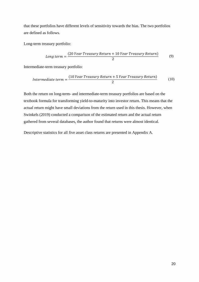
20

that these portfolios have different levels of sensitivity towards the bias. The two portfolios

are defined as follows.

Long-term treasury portfolio:

𝐿𝑜𝑛𝑔 𝑡𝑒𝑟𝑚 =(20 𝑌𝑒𝑎𝑟 𝑇𝑟𝑒𝑎𝑠𝑢𝑟𝑦 𝑅𝑒𝑡𝑢𝑟𝑛 + 10 𝑌𝑒𝑎𝑟 𝑇𝑟𝑒𝑎𝑠𝑢𝑟𝑦 𝑅𝑒𝑡𝑢𝑟𝑛)

2 (9)

Intermediate-term treasury portfolio:

𝐼𝑛𝑡𝑒𝑟𝑚𝑒𝑑𝑖𝑎𝑡𝑒 𝑡𝑒𝑟𝑚 =(10 𝑌𝑒𝑎𝑟 𝑇𝑟𝑒𝑎𝑠𝑢𝑟𝑦 𝑅𝑒𝑡𝑢𝑟𝑛 + 5 𝑌𝑒𝑎𝑟 𝑇𝑟𝑒𝑎𝑠𝑢𝑟𝑦 𝑅𝑒𝑡𝑢𝑟𝑛)

2 (10)

Both the return on long-term- and intermediate-term treasury portfolios are based on the

textbook formula for transforming yield-to-maturity into investor return. This means that the

actual return might have small deviations from the return used in this thesis. However, when

Swinkels (2019) conducted a comparison of the estimated return and the actual return

gathered from several databases, the author found that returns were almost identical.

Descriptive statistics for all five asset class returns are presented in Appendix A.

21

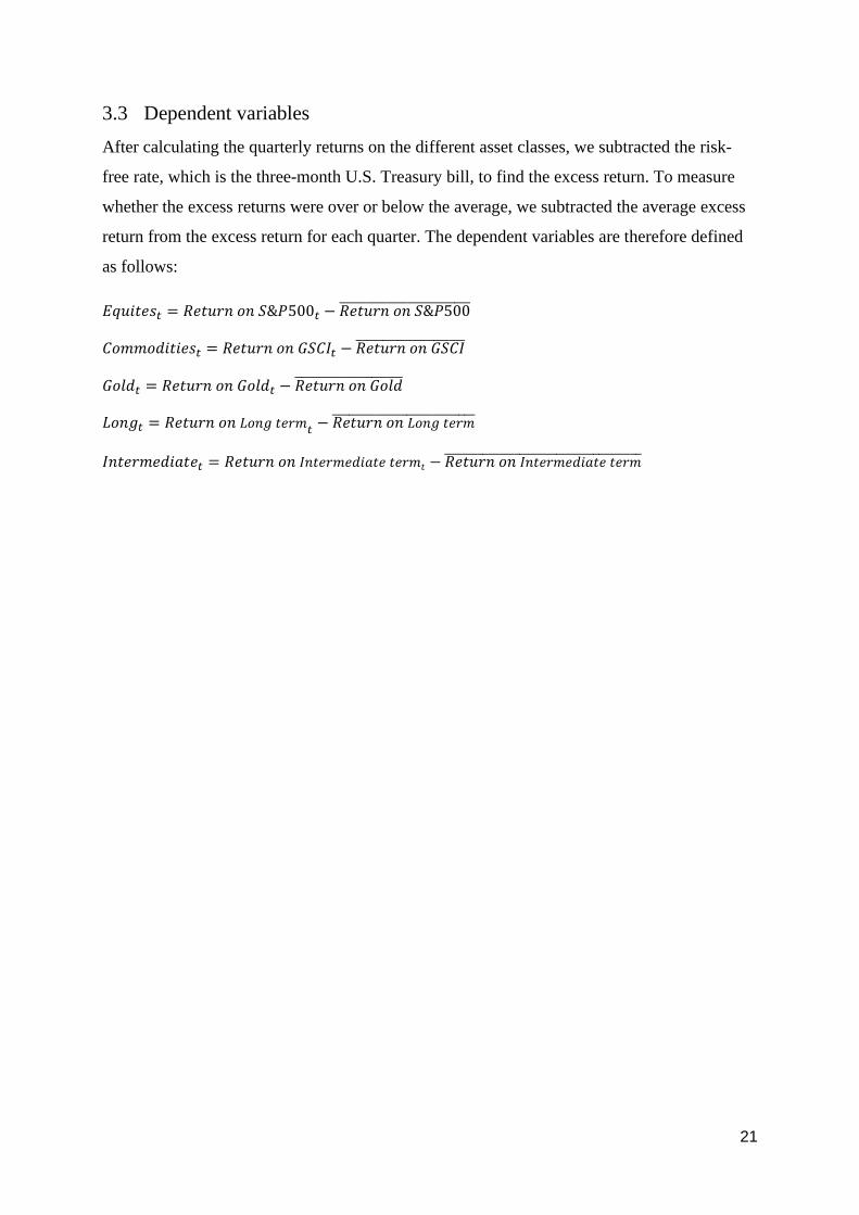
3.3 Dependent variables

After calculating the quarterly returns on the different asset classes, we subtracted the risk-

free rate, which is the three-month U.S. Treasury bill, to find the excess return. To measure

whether the excess returns were over or below the average, we subtracted the average excess

return from the excess return for each quarter. The dependent variables are therefore defined

as follows:

𝐸𝑞𝑢𝑖𝑡𝑒𝑠𝑡 = 𝑅𝑒𝑡𝑢𝑟𝑛 𝑜𝑛 𝑆&𝑃500𝑡 − 𝑅𝑒𝑡𝑢𝑟𝑛 𝑜𝑛 𝑆&𝑃500̅̅ ̅̅ ̅̅ ̅̅ ̅̅ ̅̅ ̅̅ ̅̅ ̅̅ ̅̅ ̅̅ ̅̅ ̅

𝐶𝑜𝑚𝑚𝑜𝑑𝑖𝑡𝑖𝑒𝑠𝑡 = 𝑅𝑒𝑡𝑢𝑟𝑛 𝑜𝑛 𝐺𝑆𝐶𝐼𝑡 − 𝑅𝑒𝑡𝑢𝑟𝑛 𝑜𝑛 𝐺𝑆𝐶𝐼̅̅ ̅̅ ̅̅ ̅̅ ̅̅ ̅̅ ̅̅ ̅̅ ̅̅ ̅̅ ̅

𝐺𝑜𝑙𝑑𝑡 = 𝑅𝑒𝑡𝑢𝑟𝑛 𝑜𝑛 𝐺𝑜𝑙𝑑𝑡 − 𝑅𝑒𝑡𝑢𝑟𝑛 𝑜𝑛 𝐺𝑜𝑙𝑑̅̅ ̅̅ ̅̅ ̅̅ ̅̅ ̅̅ ̅̅ ̅̅ ̅̅ ̅̅ ̅

𝐿𝑜𝑛𝑔𝑡 = 𝑅𝑒𝑡𝑢𝑟𝑛 𝑜𝑛 𝐿𝑜𝑛𝑔 𝑡𝑒𝑟𝑚𝑡 − 𝑅𝑒𝑡𝑢𝑟𝑛 𝑜𝑛 𝐿𝑜𝑛𝑔 𝑡𝑒𝑟𝑚̅̅ ̅̅ ̅̅ ̅̅ ̅̅ ̅̅ ̅̅ ̅̅ ̅̅ ̅̅ ̅̅ ̅̅ ̅̅ ̅

𝐼𝑛𝑡𝑒𝑟𝑚𝑒𝑑𝑖𝑎𝑡𝑒𝑡 = 𝑅𝑒𝑡𝑢𝑟𝑛 𝑜𝑛 𝐼𝑛𝑡𝑒𝑟𝑚𝑒𝑑𝑖𝑎𝑡𝑒 𝑡𝑒𝑟𝑚𝑡 − 𝑅𝑒𝑡𝑢𝑟𝑛 𝑜𝑛 𝐼𝑛𝑡𝑒𝑟𝑚𝑒𝑑𝑖𝑎𝑡𝑒 𝑡𝑒𝑟𝑚̅̅ ̅̅ ̅̅ ̅̅ ̅̅ ̅̅ ̅̅ ̅̅ ̅̅ ̅̅ ̅̅ ̅̅ ̅̅ ̅̅ ̅̅ ̅̅ ̅̅ ̅̅ ̅

22

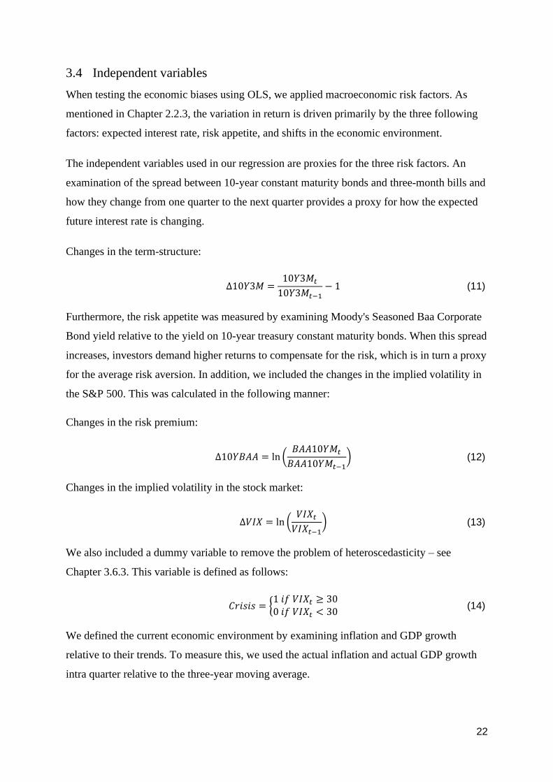
3.4 Independent variables

When testing the economic biases using OLS, we applied macroeconomic risk factors. As

mentioned in Chapter 2.2.3, the variation in return is driven primarily by the three following

factors: expected interest rate, risk appetite, and shifts in the economic environment.

The independent variables used in our regression are proxies for the three risk factors. An

examination of the spread between 10-year constant maturity bonds and three-month bills and

how they change from one quarter to the next quarter provides a proxy for how the expected

future interest rate is changing.

Changes in the term-structure:

Δ10𝑌3𝑀 =10𝑌3𝑀𝑡

10𝑌3𝑀𝑡−1− 1 (11)

Furthermore, the risk appetite was measured by examining Moody's Seasoned Baa Corporate

Bond yield relative to the yield on 10-year treasury constant maturity bonds. When this spread

increases, investors demand higher returns to compensate for the risk, which is in turn a proxy

for the average risk aversion. In addition, we included the changes in the implied volatility in

the S&P 500. This was calculated in the following manner:

Changes in the risk premium:

Δ10𝑌𝐵𝐴𝐴 = ln (𝐵𝐴𝐴10𝑌𝑀𝑡

𝐵𝐴𝐴10𝑌𝑀𝑡−1) (12)

Changes in the implied volatility in the stock market:

Δ𝑉𝐼𝑋 = ln (𝑉𝐼𝑋𝑡

𝑉𝐼𝑋𝑡−1) (13)

We also included a dummy variable to remove the problem of heteroscedasticity – see

Chapter 3.6.3. This variable is defined as follows:

𝐶𝑟𝑖𝑠𝑖𝑠 = {1 𝑖𝑓 𝑉𝐼𝑋𝑡 ≥ 300 𝑖𝑓 𝑉𝐼𝑋𝑡 < 30

(14)

We defined the current economic environment by examining inflation and GDP growth

relative to their trends. To measure this, we used the actual inflation and actual GDP growth

intra quarter relative to the three-year moving average.

23

Actual inflation:

𝐴𝑐𝑡𝑢𝑎𝑙 𝑖𝑛𝑓𝑙𝑎𝑡𝑖𝑜𝑛 = 𝑙𝑛 (𝐶𝑜𝑛𝑠𝑢𝑚𝑒𝑟 𝑃𝑟𝑖𝑐𝑒 𝐼𝑛𝑑𝑒𝑥𝑡

𝐶𝑜𝑛𝑠𝑢𝑚𝑒𝑟 𝑃𝑟𝑖𝑐𝑒 𝐼𝑛𝑑𝑒𝑥𝑡−1) (15)

Actual GDP growth:

𝐴𝑐𝑡𝑢𝑎𝑙 𝐺𝐷𝑃 𝐺𝑟𝑜𝑤𝑡ℎ = ln (𝑅𝑒𝑎𝑙 𝐺𝑟𝑜𝑠𝑠 𝐷𝑜𝑚𝑒𝑠𝑡𝑖𝑐 𝑃𝑟𝑜𝑑𝑢𝑐𝑡𝑡

𝑅𝑒𝑎𝑙 𝐺𝑟𝑜𝑠𝑠 𝐷𝑜𝑚𝑒𝑠𝑡𝑖𝑐 𝑃𝑟𝑜𝑑𝑢𝑐𝑡𝑡−1) (16)

Actual inflation relative to trend:

𝑀𝐴_𝐼𝑛𝑓𝑙𝑎𝑡𝑖𝑜𝑛12 =∑ 𝐴𝑐𝑡𝑢𝑎𝑙 𝑖𝑛𝑓𝑙𝑎𝑡𝑖𝑜𝑛𝑖

12𝑖=1

12 (17)

𝐴𝐼𝑀𝑇 = 𝐴𝑐𝑡𝑢𝑎𝑙 𝑖𝑛𝑓𝑙𝑎𝑡𝑖𝑜𝑛 − 𝑀𝐴_𝐼𝑛𝑓𝑙𝑎𝑡𝑖𝑜𝑛12 (18)

Actual GDP growth relative to trend:

𝑀𝐴_𝐺𝐷𝑃12 =∑ 𝐴𝑐𝑡𝑢𝑎𝑙 𝐺𝐷𝑃 𝐺𝑟𝑜𝑤𝑡ℎ𝑖

12𝑖=1

12 (19)

𝐴𝐺𝑀𝑇 = 𝐴𝑐𝑡𝑢𝑎𝑙 𝐺𝐷𝑃 𝐺𝑟𝑜𝑤𝑡ℎ − 𝑀𝐴_𝐺𝐷𝑃12 (20)

Actual inflation and GDP growth relative to the moving average were applied in the equation

because the present trend is approximately the same as the expectation; since most people

expect the future to closely resemble the current trend (Shahidi, 2014). However, we need to

emphasize that using the current trend as a measure for the expected inflation and GDP

growth is not perfect. This is because big movements in inflation and GDP growth during the

last three years can have big impacts on the moving average, which may lead to the current

trend not representing investors' expectations.

24

3.5 Construction and backtesting of the all-weather portfolio

This chapter presents how we constructed an all-weather portfolio with risk parity principals.

Furthermore, we present the calculations of historical return and different risk- and

drawdowns measures which were used to compare the all-weather portfolio with a 60/40 and

all-equity portfolio.

3.5.1 Construction of the all-weather portfolio

Bridgewater Associates asset allocation is not publicly available. This thesis therefore uses the

asset classes that were included in the simplified version of the all-weather portfolio – the ‘all-

season portfolio’ – which was popularized by Tony Robbins in his book Money: Master the

Game (Robbins, 2014). To determine the weights of the different asset classes in the portfolio

we applied a risk factor parity approach.

Figure 3.1 - The four economic states

Based on the most important macroeconomic risk factors – inflation and economic growth –

we divided the economy into four possible economic states, as illustrated in Figure 3.1 above.

Table 3.1 - Asset class bias and preferred economic states

Asset class bias Inflation is GDP Growth is

GSCI should do better when: Higher than expected Higher than expected

Gold should do better when: Higher than expected Lower than expected

S&P 500 should do better when: Lower than expected Higher than expected

Long-term treasuries should do better when: Lower than expected Lower than expected

Intermediate-term treasuries should do better when: Lower than expected Lower than expected

The expected economical biases for the five different asset classes – as discussed in Chapter

2.2.4 – are summarized in Table 3.1 above. The preferred economic states are found by

combining the economic biases of the different asset classes; this also implies that the worst

economic state is the state with the opposite values for inflation and GDP growth.

25

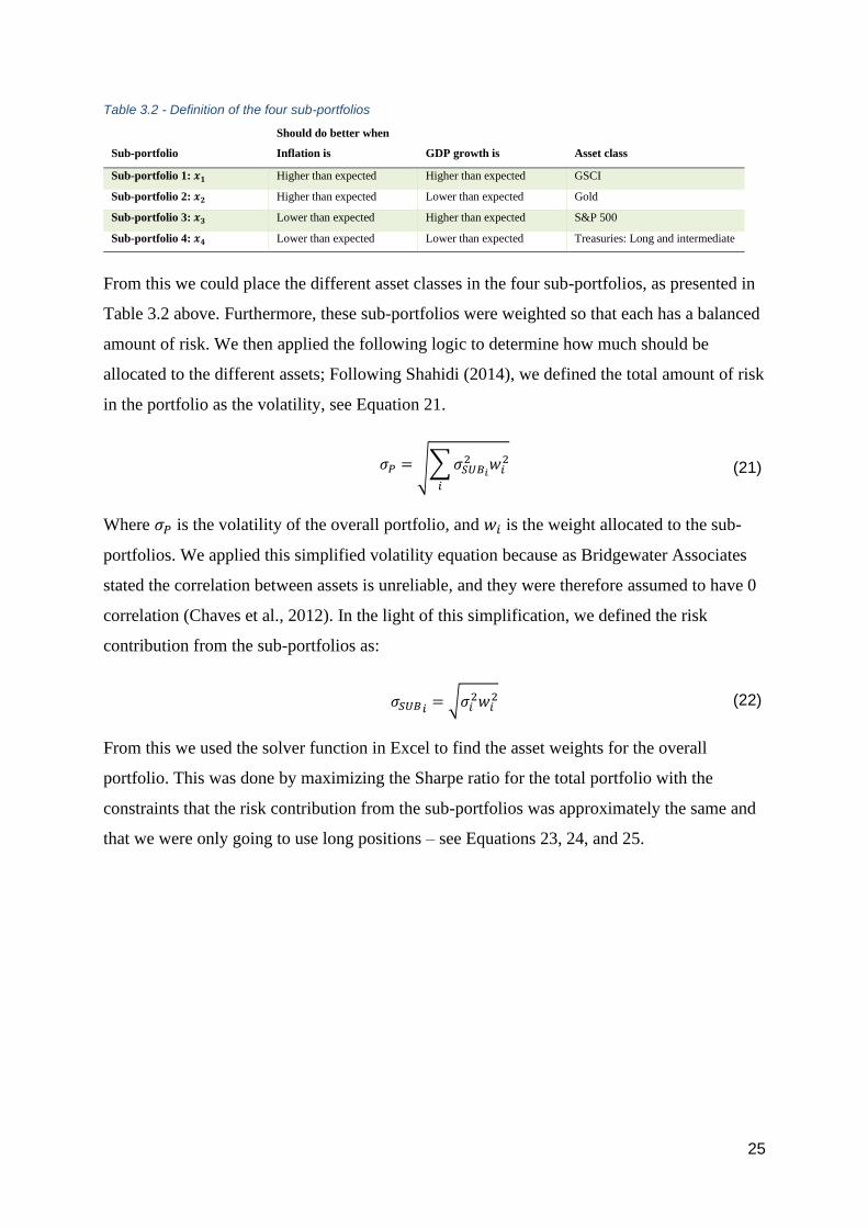
Table 3.2 - Definition of the four sub-portfolios

Sub-portfolio

Should do better when

Inflation is

GDP growth is

Asset class

Sub-portfolio 1: 𝒙𝟏 Higher than expected Higher than expected GSCI

Sub-portfolio 2: 𝒙𝟐 Higher than expected Lower than expected Gold

Sub-portfolio 3: 𝒙𝟑 Lower than expected Higher than expected S&P 500

Sub-portfolio 4: 𝒙𝟒 Lower than expected Lower than expected Treasuries: Long and intermediate

From this we could place the different asset classes in the four sub-portfolios, as presented in

Table 3.2 above. Furthermore, these sub-portfolios were weighted so that each has a balanced

amount of risk. We then applied the following logic to determine how much should be

allocated to the different assets; Following Shahidi (2014), we defined the total amount of risk

in the portfolio as the volatility, see Equation 21.

𝜎𝑃 = √∑ 𝜎𝑆𝑈𝐵𝑖

2 𝑤𝑖2

𝑖

(21)

Where 𝜎𝑃 is the volatility of the overall portfolio, and 𝑤𝑖 is the weight allocated to the sub-

portfolios. We applied this simplified volatility equation because as Bridgewater Associates

stated the correlation between assets is unreliable, and they were therefore assumed to have 0

correlation (Chaves et al., 2012). In the light of this simplification, we defined the risk

contribution from the sub-portfolios as:

𝜎𝑆𝑈𝐵𝑖= √𝜎𝑖

2𝑤𝑖2 (22)

From this we used the solver function in Excel to find the asset weights for the overall

portfolio. This was done by maximizing the Sharpe ratio for the total portfolio with the

constraints that the risk contribution from the sub-portfolios was approximately the same and

that we were only going to use long positions – see Equations 23, 24, and 25.

26

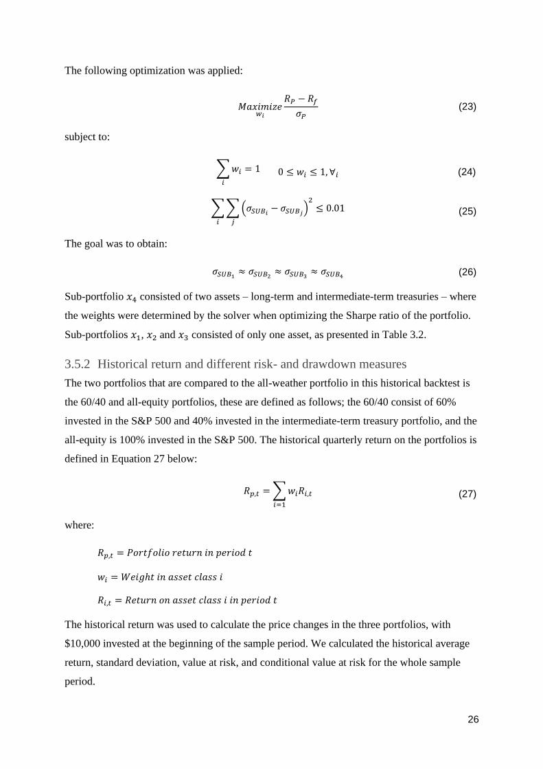
The following optimization was applied:

𝑀𝑎𝑥𝑖𝑚𝑖𝑧𝑒𝑤𝑖

𝑅𝑃 − 𝑅𝑓

𝜎𝑃 (23)

subject to:

∑ 𝑤𝑖 = 1

𝑖

0 ≤ 𝑤𝑖 ≤ 1, ∀𝑖 (24)

∑ ∑ (𝜎𝑆𝑈𝐵𝑖− 𝜎𝑆𝑈𝐵𝑗

)2

≤ 0.01

𝑗𝑖

(25)

The goal was to obtain:

𝜎𝑆𝑈𝐵1≈ 𝜎𝑆𝑈𝐵2

≈ 𝜎𝑆𝑈𝐵3≈ 𝜎𝑆𝑈𝐵4

(26)

Sub-portfolio 𝑥4 consisted of two assets – long-term and intermediate-term treasuries – where

the weights were determined by the solver when optimizing the Sharpe ratio of the portfolio.

Sub-portfolios 𝑥1, 𝑥2 and 𝑥3 consisted of only one asset, as presented in Table 3.2.

3.5.2 Historical return and different risk- and drawdown measures

The two portfolios that are compared to the all-weather portfolio in this historical backtest is

the 60/40 and all-equity portfolios, these are defined as follows; the 60/40 consist of 60%

invested in the S&P 500 and 40% invested in the intermediate-term treasury portfolio, and the

all-equity is 100% invested in the S&P 500. The historical quarterly return on the portfolios is

defined in Equation 27 below:

𝑅𝑝,𝑡 = ∑ 𝑤𝑖𝑅𝑖,𝑡

𝑖=1

(27)

where:

𝑅𝑝,𝑡 = 𝑃𝑜𝑟𝑡𝑓𝑜𝑙𝑖𝑜 𝑟𝑒𝑡𝑢𝑟𝑛 𝑖𝑛 𝑝𝑒𝑟𝑖𝑜𝑑 𝑡

𝑤𝑖 = 𝑊𝑒𝑖𝑔ℎ𝑡 𝑖𝑛 𝑎𝑠𝑠𝑒𝑡 𝑐𝑙𝑎𝑠𝑠 𝑖

𝑅𝑖,𝑡 = 𝑅𝑒𝑡𝑢𝑟𝑛 𝑜𝑛 𝑎𝑠𝑠𝑒𝑡 𝑐𝑙𝑎𝑠𝑠 𝑖 𝑖𝑛 𝑝𝑒𝑟𝑖𝑜𝑑 𝑡

The historical return was used to calculate the price changes in the three portfolios, with

$10,000 invested at the beginning of the sample period. We calculated the historical average

return, standard deviation, value at risk, and conditional value at risk for the whole sample

period.

27

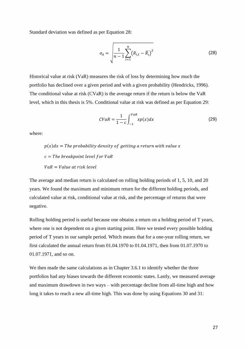
Standard deviation was defined as per Equation 28:

𝜎𝐴 = √1

𝑛 − 1∑(𝑅𝑖,𝑡 − 𝑅�̅�)

2𝑛

𝑖=1

(28)

Historical value at risk (VaR) measures the risk of loss by determining how much the

portfolio has declined over a given period and with a given probability (Hendricks, 1996).

The conditional value at risk (CVaR) is the average return if the return is below the VaR

level, which in this thesis is 5%. Conditional value at risk was defined as per Equation 29:

𝐶𝑉𝑎𝑅 =1

1 − 𝑐∫ 𝑥𝑝(𝑥)𝑑𝑥

𝑉𝑎𝑅

−1

(29)

where:

𝑝(𝑥)𝑑𝑥 = 𝑇ℎ𝑒 𝑝𝑟𝑜𝑏𝑎𝑏𝑖𝑙𝑖𝑡𝑦 𝑑𝑒𝑛𝑠𝑖𝑡𝑦 𝑜𝑓 𝑔𝑒𝑡𝑡𝑖𝑛𝑔 𝑎 𝑟𝑒𝑡𝑢𝑟𝑛 𝑤𝑖𝑡ℎ 𝑣𝑎𝑙𝑢𝑒 𝑥

𝑐 = 𝑇ℎ𝑒 𝑏𝑟𝑒𝑎𝑘𝑝𝑜𝑖𝑛𝑡 𝑙𝑒𝑣𝑒𝑙 𝑓𝑜𝑟 𝑉𝑎𝑅

𝑉𝑎𝑅 = 𝑉𝑎𝑙𝑢𝑒 𝑎𝑡 𝑟𝑖𝑠𝑘 𝑙𝑒𝑣𝑒𝑙

The average and median return is calculated on rolling holding periods of 1, 5, 10, and 20

years. We found the maximum and minimum return for the different holding periods, and

calculated value at risk, conditional value at risk, and the percentage of returns that were

negative.

Rolling holding period is useful because one obtains a return on a holding period of T years,

where one is not dependent on a given starting point. Here we tested every possible holding

period of T years in our sample period. Which means that for a one-year rolling return, we

first calculated the annual return from 01.04.1970 to 01.04.1971, then from 01.07.1970 to

01.07.1971, and so on.

We then made the same calculations as in Chapter 3.6.1 to identify whether the three

portfolios had any biases towards the different economic states. Lastly, we measured average

and maximum drawdown in two ways – with percentage decline from all-time high and how

long it takes to reach a new all-time high. This was done by using Equations 30 and 31:

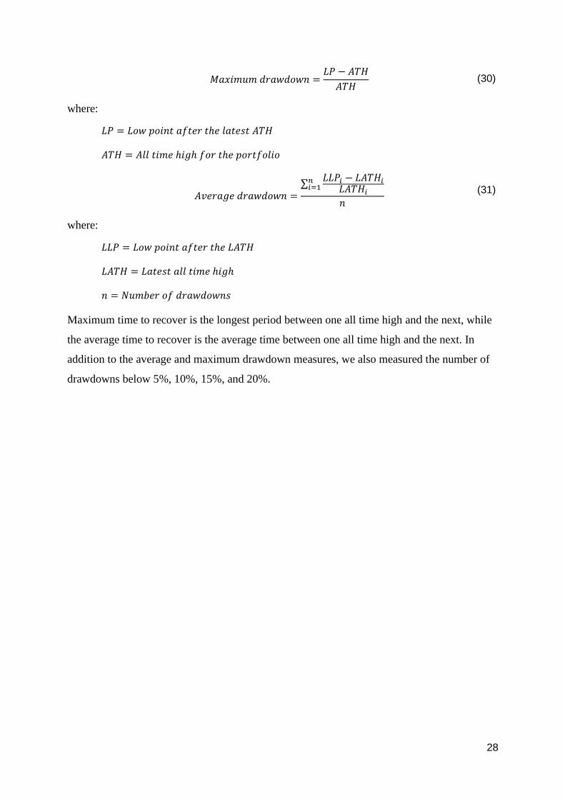
28

𝑀𝑎𝑥𝑖𝑚𝑢𝑚 𝑑𝑟𝑎𝑤𝑑𝑜𝑤𝑛 =𝐿𝑃 − 𝐴𝑇𝐻

𝐴𝑇𝐻 (30)

where:

𝐿𝑃 = 𝐿𝑜𝑤 𝑝𝑜𝑖𝑛𝑡 𝑎𝑓𝑡𝑒𝑟 𝑡ℎ𝑒 𝑙𝑎𝑡𝑒𝑠𝑡 𝐴𝑇𝐻

𝐴𝑇𝐻 = 𝐴𝑙𝑙 𝑡𝑖𝑚𝑒 ℎ𝑖𝑔ℎ 𝑓𝑜𝑟 𝑡ℎ𝑒 𝑝𝑜𝑟𝑡𝑓𝑜𝑙𝑖𝑜

𝐴𝑣𝑒𝑟𝑎𝑔𝑒 𝑑𝑟𝑎𝑤𝑑𝑜𝑤𝑛 =

∑𝐿𝐿𝑃𝑖 − 𝐿𝐴𝑇𝐻𝑖

𝐿𝐴𝑇𝐻𝑖

𝑛𝑖=1

𝑛

(31)

where:

𝐿𝐿𝑃 = 𝐿𝑜𝑤 𝑝𝑜𝑖𝑛𝑡 𝑎𝑓𝑡𝑒𝑟 𝑡ℎ𝑒 𝐿𝐴𝑇𝐻

𝐿𝐴𝑇𝐻 = 𝐿𝑎𝑡𝑒𝑠𝑡 𝑎𝑙𝑙 𝑡𝑖𝑚𝑒 ℎ𝑖𝑔ℎ

𝑛 = 𝑁𝑢𝑚𝑏𝑒𝑟 𝑜𝑓 𝑑𝑟𝑎𝑤𝑑𝑜𝑤𝑛𝑠

Maximum time to recover is the longest period between one all time high and the next, while

the average time to recover is the average time between one all time high and the next. In

addition to the average and maximum drawdown measures, we also measured the number of

drawdowns below 5%, 10%, 15%, and 20%.

29

3.6 Testing for asset class bias

This chapter presents how we tested for asset class bias. First, we calculated the historical

average return on the different asset classes in periods when inflation and GDP growth were

higher or lower than the three-year moving average. We further examined asset class bias

using OLS regressions to test whether the different asset classes had the expected sign on the

beta coefficients.

3.6.1 Average return tests

Historical arithmetic average returns were calculated on the five different asset classes on a

quarterly basis for the whole sample period. We then calculated the historical average return

in periods of high or low inflation and economic growth, both separately and combined.

Thereby testing whether the assets have a bias toward the two risk factors, and if the assets

perform differently in the four different economic states. The four economic biases are

presented in Table 3.3 below.

Table 3.3 - Description of the four economic biases

Description of the four economic biases

Bias 1: Higher than expected inflation

Bias 2: Lower than expected inflation

Bias 3: Higher than expected GDP growth

Bias 4: Lower than expected GDP growth

Finally, we combined the measurements on inflation and GDP growth so that the economy

consisted of the four states presented in Table 3.4 below.

Table 3.4 - Description of the four economic states

Description of the four economic states Inflation is: GDP Growth is:

Economic state 1: Higher than expected Higher than expected

Economic state 2: Higher than expected Lower than expected

Economic state 3: Lower than expected Higher than expected

Economic state 4: Lower than expected Lower than expected

This made it possible to measure whether the different assets, on average, perform better in

the economic states defined in this chapter.

In addition, we tested the robustness of this test by dividing the sample period into two sub-

periods: the first period from 01.04.1970 to 01.10.1994, and the second from 01.01.1995 to

01.01.2021. We then repeated the test described in this chapter on the sub-holding periods.

30

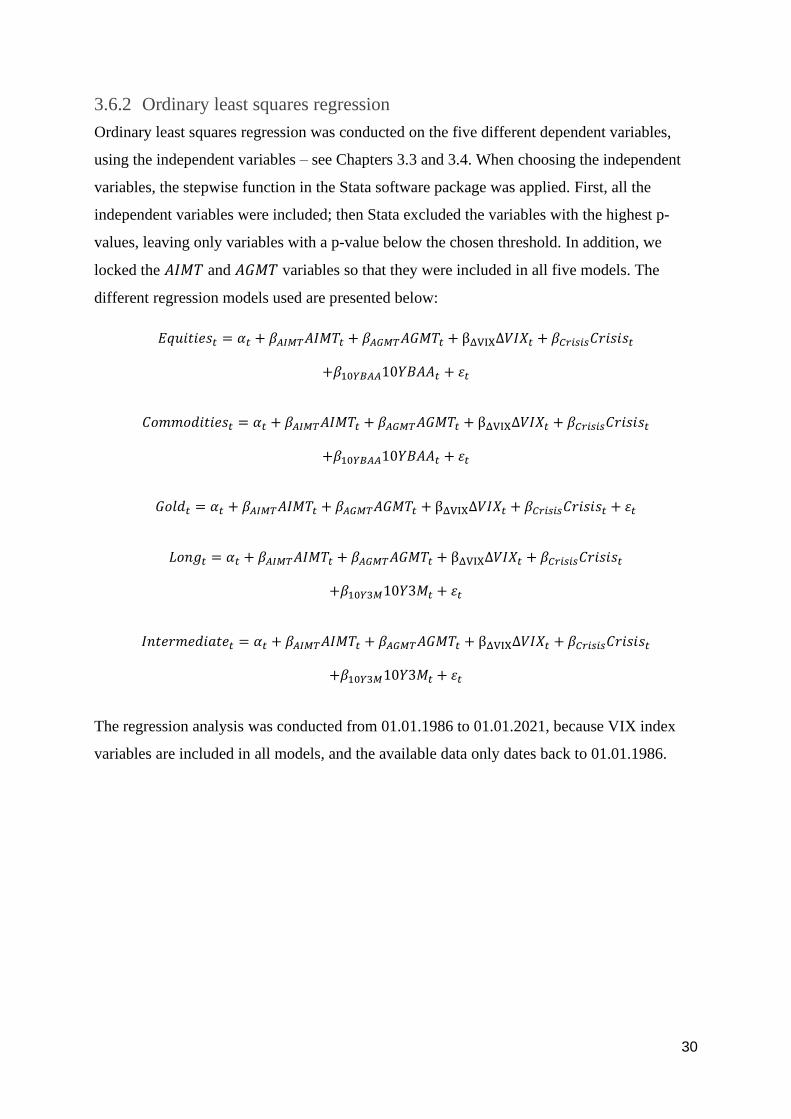
3.6.2 Ordinary least squares regression

Ordinary least squares regression was conducted on the five different dependent variables,

using the independent variables – see Chapters 3.3 and 3.4. When choosing the independent

variables, the stepwise function in the Stata software package was applied. First, all the

independent variables were included; then Stata excluded the variables with the highest p-

values, leaving only variables with a p-value below the chosen threshold. In addition, we

locked the 𝐴𝐼𝑀𝑇 and 𝐴𝐺𝑀𝑇 variables so that they were included in all five models. The

different regression models used are presented below:

𝐸𝑞𝑢𝑖𝑡𝑖𝑒𝑠𝑡 = 𝛼𝑡 + 𝛽𝐴𝐼𝑀𝑇𝐴𝐼𝑀𝑇𝑡 + 𝛽𝐴𝐺𝑀𝑇𝐴𝐺𝑀𝑇𝑡 + βΔVIXΔ𝑉𝐼𝑋𝑡 + 𝛽𝐶𝑟𝑖𝑠𝑖𝑠𝐶𝑟𝑖𝑠𝑖𝑠𝑡

+𝛽10𝑌𝐵𝐴𝐴10𝑌𝐵𝐴𝐴𝑡 + 𝜀𝑡

𝐶𝑜𝑚𝑚𝑜𝑑𝑖𝑡𝑖𝑒𝑠𝑡 = 𝛼𝑡 + 𝛽𝐴𝐼𝑀𝑇𝐴𝐼𝑀𝑇𝑡 + 𝛽𝐴𝐺𝑀𝑇𝐴𝐺𝑀𝑇𝑡 + βΔVIXΔ𝑉𝐼𝑋𝑡 + 𝛽𝐶𝑟𝑖𝑠𝑖𝑠𝐶𝑟𝑖𝑠𝑖𝑠𝑡

+𝛽10𝑌𝐵𝐴𝐴10𝑌𝐵𝐴𝐴𝑡 + 𝜀𝑡

𝐺𝑜𝑙𝑑𝑡 = 𝛼𝑡 + 𝛽𝐴𝐼𝑀𝑇𝐴𝐼𝑀𝑇𝑡 + 𝛽𝐴𝐺𝑀𝑇𝐴𝐺𝑀𝑇𝑡 + βΔVIXΔ𝑉𝐼𝑋𝑡 + 𝛽𝐶𝑟𝑖𝑠𝑖𝑠𝐶𝑟𝑖𝑠𝑖𝑠𝑡 + 𝜀𝑡

𝐿𝑜𝑛𝑔𝑡 = 𝛼𝑡 + 𝛽𝐴𝐼𝑀𝑇𝐴𝐼𝑀𝑇𝑡 + 𝛽𝐴𝐺𝑀𝑇𝐴𝐺𝑀𝑇𝑡 + βΔVIXΔ𝑉𝐼𝑋𝑡 + 𝛽𝐶𝑟𝑖𝑠𝑖𝑠𝐶𝑟𝑖𝑠𝑖𝑠𝑡

+𝛽10𝑌3𝑀10𝑌3𝑀𝑡 + 𝜀𝑡

𝐼𝑛𝑡𝑒𝑟𝑚𝑒𝑑𝑖𝑎𝑡𝑒𝑡 = 𝛼𝑡 + 𝛽𝐴𝐼𝑀𝑇𝐴𝐼𝑀𝑇𝑡 + 𝛽𝐴𝐺𝑀𝑇𝐴𝐺𝑀𝑇𝑡 + βΔVIXΔ𝑉𝐼𝑋𝑡 + 𝛽𝐶𝑟𝑖𝑠𝑖𝑠𝐶𝑟𝑖𝑠𝑖𝑠𝑡

+𝛽10𝑌3𝑀10𝑌3𝑀𝑡 + 𝜀𝑡

The regression analysis was conducted from 01.01.1986 to 01.01.2021, because VIX index

variables are included in all models, and the available data only dates back to 01.01.1986.

31

3.6.3 Testing of ordinary least square assumptions

When running a regression analysis, one needs to ensure that the models are correctly

specified. To do this we tested for functional form, stationarity, autocorrelation,

heteroscedasticity, and multicollinearity. In addition, we checked whether the variables were

approximately normally distributed.

We applied the Ramsey regression equation specification error test (RESET) to determine

whether there was a high probability that the regression model was wrongly specified.

However, there were no significant specification errors – see Appendix B.1.

Stationarity means that the time series has constant mean and variance over the sample period

(Studenmund, 2017). This is an important prerequisite for obtaining reliable coefficients from

the regression.

The two-way plot in Appendices B.2 to B.6 reveals that the return on all asset classes seems

to be stationary, except gold which seem to have some problems with autocorrelation. The

independent variables have more serious problems with stationarity; inflation relative to trend

has certain large outliers which we addressed by including a dummy variable for ‘𝐶𝑟𝑖𝑠𝑖𝑠’,

where 1 indicates values over 30 on the VIX. This method mostly removes the problems with

outliers (Studenmund, 2017). GDP growth relative to trend has approximately the same mean

throughout the sample period, but it also has a large outlier during the coronavirus crisis in

2020. This problem was also solved by using the ‘𝐶𝑟𝑖𝑠𝑖𝑠’ dummy.

An examination of the absolute values on VIX, the risk premium on corporate bonds, and the

spreads between 10-year treasuries and three-month treasuries reveals that there is a

significant difference in mean and in volatility over time. This is why we examined changes

from one period to the next to deal with the non-stationarity. This yielded variables that seem

to be stationary – see Appendices B.7 to B.10.

Autocorrelation was tested by using the Durbin-Watson test and the Breusch-Godfrey test, the

results of which are presented in Appendix B.11 and demonstrate that there is no significant

autocorrelation. This is also confirmed by the correlograms in Appendix B.12.

Heteroscedasticity was tested by using the White test and the Breusch-Pagan test, the results

of which are summarized in Appendix B.13. Here it is observed that the equity model has

significant heteroscedasticity. This problem was solved by using heteroscedasticity-corrected

32

standard errors, where we adjusted the estimated standard errors for heteroscedasticity while

still using the same OLS estimated coefficients (Studenmund, 2017).

Testing for multicollinearity was done by first examining the correlation between the

independent variables. In addition, we used the VIF test in Stata, the results of which are

presented in Appendices B.14 and B.15. From the correlation matrix it is clear that there is a

0.552 correlation between the Δ𝑉𝐼𝑋 and Δ10𝑌𝐵𝐴𝐴 variables. In addition, it is observed that

there are multiple variables with a correlation around +/-032. However, the VIF table reveals

no significant multicollinearity.

Furthermore, we tested for normally distributed residuals by applying the skewness and

kurtosis test, the Shapiro-Wilk test, and the Shapiro-Francia test for normality. These results

can be reviewed in Appendix B.16. In addition, we created residual histograms – see

Appendix B.17. These tests reveal that the equity and commodity models residuals are not

normally distributed. This is not necessarily a problem, as we have a large sample size with

139 observations, and we can therefore assume normality based on the central limit theorem

(Thomas, 2005).

33

3.7 Historical risk-adjusted returns for the different asset classes

In one of the Bridgewater Associates research papers it is stated that, ‘in risk-adjusted terms

asset classes have roughly equivalent returns’ (Jensen & Rotenberg, 2004, p. 3). This is tested

by calculating the Sharpe ratio for the different asset classes (i.e., how much return received

per unit of risk). The reason this is an important assumption is that if asset classes have

different Sharpe ratios, the allocation method based on risk alone will give some parts of the

portfolio a lower expected return than others.

The historical Sharpe ratio is calculated by subtracting the risk-free rate of return 𝑅𝑓 from the

expected asset class return 𝑅𝐴 over a given period, which is then divided by the standard

deviation (volatility) of the expected asset class return 𝜎𝐴 during the same period – the

standard deviation is defined in Equation 28. We used the quarterly returns in the manner

explained in Chapter 3.2, the risk-free rate is the quarterly treasury bill yield, and the Sharpe

ratio was calculated on a quarterly basis as presented in Equation 32. Next, we identified the

average values for the Sharpe ratio, for the whole sample period and for the five individual

decades.

The Sharpe ratio was defined as per Equation 32:

𝑆ℎ𝑎𝑟𝑝𝑒 𝑟𝑎𝑡𝑖𝑜 =𝑅𝐴 − 𝑅𝑓

𝜎𝐴 (32)

34

4 Empirical results and discussion

This chapter presents the results of our analysis. The main purpose of this thesis is to examine

how the all-weather portfolio performs compared to the 60/40 and all-equity portfolios, and if

the assumptions for the all-weather portfolio are valid. First, we present the results from the

construction of the portfolio and the backtesting with a comparison to 60/40 and all-equity

portfolios. Second, the test of assumed asset class bias towards defined economic risk factors

are presented. Finally, we present the risk-adjusted return test for the different asset classes.

4.1 Results from construction and backtesting of the all-weather portfolio

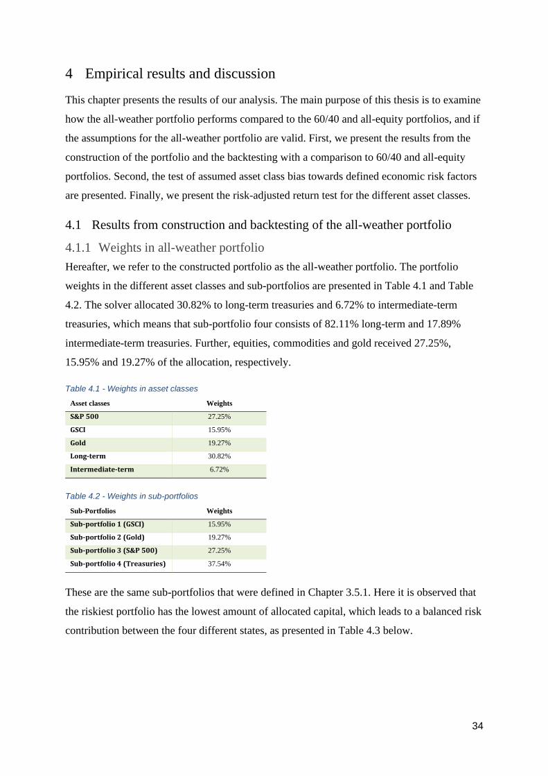
4.1.1 Weights in all-weather portfolio

Hereafter, we refer to the constructed portfolio as the all-weather portfolio. The portfolio

weights in the different asset classes and sub-portfolios are presented in Table 4.1 and Table

4.2. The solver allocated 30.82% to long-term treasuries and 6.72% to intermediate-term

treasuries, which means that sub-portfolio four consists of 82.11% long-term and 17.89%

intermediate-term treasuries. Further, equities, commodities and gold received 27.25%,

15.95% and 19.27% of the allocation, respectively.

Table 4.1 - Weights in asset classes

Asset classes Weights

S&P 500 27.25%

GSCI 15.95%

Gold 19.27%

Long-term 30.82%

Intermediate-term 6.72%

Table 4.2 - Weights in sub-portfolios

Sub-Portfolios Weights

Sub-portfolio 1 (GSCI) 15.95%

Sub-portfolio 2 (Gold) 19.27%

Sub-portfolio 3 (S&P 500) 27.25%

Sub-portfolio 4 (Treasuries) 37.54%

These are the same sub-portfolios that were defined in Chapter 3.5.1. Here it is observed that

the riskiest portfolio has the lowest amount of allocated capital, which leads to a balanced risk

contribution between the four different states, as presented in Table 4.3 below.

35

Table 4.3 - Risk balance between economic states

Economic states Risk contribution

State 1 – High/High 24.64%

State 2 – High/Low 25.00%

State 3 – Low/High 24.86%

State 4 – Low/Low 25.50%

Table 4.4 below indicates that the portfolio also has a balanced allocation on both

macroeconomic risk factors, where the portfolio has approximately the same amount of risk in

higher-than-expected and lower-than-expected inflation and GDP growth.

Table 4.4 - Risk balance between economic biases

Economical biases Risk contribution

High inflation 24.82%

Low inflation 25.18%

High GDP growth 24.75%

Low GDP growth 25.25%

36

4.1.2 Historical return and different risk- and drawdown measures

4.1.2.1 Historical return and risk measures

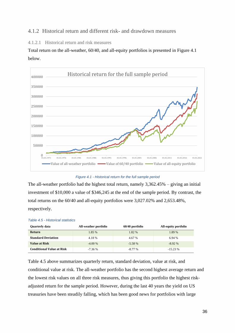
Total return on the all-weather, 60/40, and all-equity portfolios is presented in Figure 4.1

below.

Figure 4.1 - Historical return for the full sample period

The all-weather portfolio had the highest total return, namely 3,362.45% – giving an initial

investment of $10,000 a value of $346,245 at the end of the sample period. By contrast, the

total returns on the 60/40 and all-equity portfolios were 3,027.02% and 2,653.48%,

respectively.

Table 4.5 - Historical statistics

Quarterly data All-weather portfolio 60/40 portfolio All-equity portfolio

Return 1.85 % 1.82 % 1.89 %

Standard Deviation 4.18 % 4.67 % 6.94 %

Value at Risk -4.00 % -5.58 % -8.92 %

Conditional Value at Risk -7.36 % -8.77 % -15.23 %

Table 4.5 above summarizes quarterly return, standard deviation, value at risk, and

conditional value at risk. The all-weather portfolio has the second highest average return and

the lowest risk values on all three risk measures, thus giving this portfolio the highest risk-

adjusted return for the sample period. However, during the last 40 years the yield on US

treasuries have been steadily falling, which has been good news for portfolios with large

0

50000

100000

150000

200000

250000

300000

350000

400000

01.01.1971 01.01.1976 01.01.1981 01.01.1986 01.01.1991 01.01.1996 01.01.2001 01.01.2006 01.01.2011 01.01.2016 01.01.2021

Historical return for the full sample period

Value of all-weather portfolio Value of 60/40 portfolio Value of all-equity portfolio

37

allocation to US Treasuries, such as the all-weather and 60/40 portfolio. The high return on

these portfolios may however not be replicable in the future as we cannot expect the yield to

fall much further.

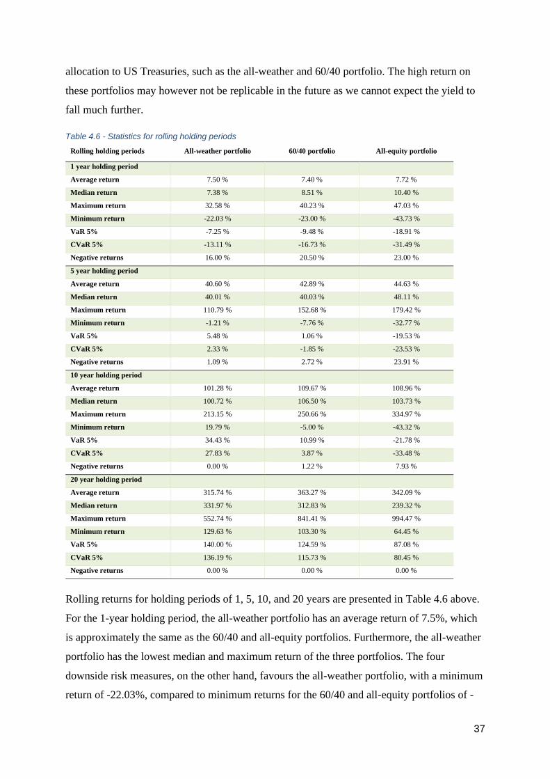
Table 4.6 - Statistics for rolling holding periods

Rolling holding periods All-weather portfolio 60/40 portfolio All-equity portfolio

1 year holding period

Average return 7.50 % 7.40 % 7.72 %

Median return 7.38 % 8.51 % 10.40 %

Maximum return 32.58 % 40.23 % 47.03 %

Minimum return -22.03 % -23.00 % -43.73 %

VaR 5% -7.25 % -9.48 % -18.91 %

CVaR 5% -13.11 % -16.73 % -31.49 %

Negative returns 16.00 % 20.50 % 23.00 %


Average return 40.60 % 42.89 % 44.63 %

Median return 40.01 % 40.03 % 48.11 %

Maximum return 110.79 % 152.68 % 179.42 %

Minimum return -1.21 % -7.76 % -32.77 %

VaR 5% 5.48 % 1.06 % -19.53 %

CVaR 5% 2.33 % -1.85 % -23.53 %



Average return 101.28 % 109.67 % 108.96 %

Median return 100.72 % 106.50 % 103.73 %

Maximum return 213.15 % 250.66 % 334.97 %

Minimum return 19.79 % -5.00 % -43.32 %

VaR 5% 34.43 % 10.99 % -21.78 %

CVaR 5% 27.83 % 3.87 % -33.48 %



Average return 315.74 % 363.27 % 342.09 %

Median return 331.97 % 312.83 % 239.32 %

Maximum return 552.74 % 841.41 % 994.47 %

Minimum return 129.63 % 103.30 % 64.45 %

VaR 5% 140.00 % 124.59 % 87.08 %

CVaR 5% 136.19 % 115.73 % 80.45 %


Rolling returns for holding periods of 1, 5, 10, and 20 years are presented in Table 4.6 above.

For the 1-year holding period, the all-weather portfolio has an average return of 7.5%, which

is approximately the same as the 60/40 and all-equity portfolios. Furthermore, the all-weather

portfolio has the lowest median and maximum return of the three portfolios. The four

downside risk measures, on the other hand, favours the all-weather portfolio, with a minimum

return of -22.03%, compared to minimum returns for the 60/40 and all-equity portfolios of -

38

23% and -43.73%, respectively. Moreover, the all-weather portfolio has the highest VaR 5%

and CVaR 5% (i.e., less risk), with a negative return only 16% of the time.

The 5- and 10-year holding periods display a similar result, where the average, median, and

maximum return is approximately the same or lower for the all-weather portfolio, but the

downside risk is significantly lower.

When the holding period is increased to 20 years, the average return is lowest for the all-

weather portfolio, but it has the highest median return. Furthermore, the all-weather portfolio

has a much lower maximum return. However, the downside risk is lower, as indicated by the

minimum return, VaR 5% and CVaR 5% measurements. None of the portfolios has a negative

return when the holding period is increased to 20 years.

Tests of the average return with asset class biases towards economic growth and inflation

revealed that the all-weather portfolio deviates least from the average return for the full

sample period – see Table 4.7 for periods with higher or lower than expected inflation and

GDP growth and Table 4.8 for periods of the four economic states.

Table 4.7 - Average excess return in periods of either high or low inflation/GDP growth

Average excess return Average excess return on

all-weather portfolio

Average excess return on

60/40 portfolio


all-equity portfolio

Full sample

Average excess return 0.71 % 0.68 % 0.76 %

Inflation is

Higher than expected


Lower than expected


GDP growth is



Lower than expected

Average excess return 0.91 % 0.40 % -0.19 %

From Table 4.7 above we can see that the largest deviation for the three portfolios is

approximately ±0.20% for the all-weather portfolio, approximately ±0.60% for the 60/40

portfolio, and approximately ±0.90% for the all-equity portfolio. Indicating that the all-

weather portfolio has less economical bias.

39

Table 4.8 - Average excess return in the four economic states

Average excess return Average excess return on

all-weather portfolio


60/40 portfolio


all-equity portfolio

Full sample


High inflation/ High GDP growth


High inflation/ Low GDP growth

Average excess return 1.41 % -0.21 % -0.86 %

Low inflation/ High GDP growth


Low inflation/ Low GDP growth


It is clear from Table 4.8 above that the all-weather portfolio performs best in the state with

high inflation/low GDP growth and performs poorest in the high inflation/ high GDP growth

state. Although there is a larger deviation in returns between these four states, the all-weather

portfolio has less variation in returns and the poorest performing state for this portfolio is

better than the poorest performing state for the two other portfolios.

40

4.1.2.2 Drawdown measures

The drawdown charts in Figure 4.2, Figure 4.3, and Figure 4.4 indicate that there is a

significant difference in how frequently the three different portfolios are below the all-time

high. In addition, it is clear that the magnitude of the drawdown and how long it takes for the

portfolio to recover are significantly different.

Figure 4.2 - Drawdowns for the all-weather portfolio

Figure 4.3 - Drawdowns for the 60/40 portfolio

Figure 4.4 - Drawdowns for the all-equity portfolio

-60%

-50%

-40%

-30%

-20%

-10%

0%

All-weather portfolio

-60%

-50%

-40%

-30%

-20%

-10%

0%

60/40 portfolio

-60%

-50%

-40%

-30%

-20%

-10%

0%

All-equity portfolio

41

Table 4.9 - Drawdown statistical measures

Drawdown measures All-weather portfolio 60/40 portfolio All-equity portfolio

Maximum percentage drawdown -22.21% -26.85% -50.31%

Average percentage drawdown -4.99% -5.86% -11.29%

Maximum number of quarters until new all-time high 13 18 30

Average number of quarters until new all-time high 2.93 3.59 5.46

Number of drawdowns less than -5% 8 11 12




Table 4.9 confirms the view expressed above. The maximum drawdown for the all-weather

portfolio is -22.21% compared to the 60/40 and all-equity portfolios which have maximum

drawdowns of -26.85% and -50.31%, respectively. The average drawdown is also lower for

the all-weather portfolio. The maximum time to recover from a drawdown is 13 quarters, and

the average time is 2.93 quarters for the all-weather portfolio. This is significantly lower than

for the two other portfolios. Furthermore, the number of drawdowns below 5%, 10%, 15%,

and 20% is the same or lower for the all-weather portfolio.

42

4.2 Results from the economic bias tests

4.2.1 Results from average return tests

Table 4.10 presents asset class average excess returns in periods of high or low economic

growth and inflation, while Table 4.11 presents the average excess return for the economic

states. In both tables, average excess returns for each asset class are calculated for the

economic environments and the full sample period.

Table 4.10 - Average excess return in periods of either high or low inflation/GDP growth

Average excess return Excess return

S&P 500

Excess return

GSCI

Excess return

Gold

Excess return

Long-Term

Excess return

Intermediate-Term

Full sample

Average excess return 0.76 % 0.33 % 0.82 % 0.83 % 0.57 %

Inflation is


Average excess return 0.37 % 2.61 % 2.58 % -0.56 % -0.33 %

Lower than expected

Average excess return 1.10 % -1.72 % -0.75 % 2.09 % 1.39 %

GDP growth is


Average excess return 1.67 % 1.10 % -0.26 % -0.16 % -0.12 %

Lower than expected

Average excess return -0.19 % -0.46 % 1.94 % 1.85 % 1.29 %

It is clear from Table 4.10 that all asset classes have an above average excess return in the

periods when inflation and economic growth are assumed to be favourable for the different

asset classes, as defined in Table 3.1. With an average return of 1.10% and 1.67%, the results

indicate that equities are biased towards performing above average when inflation is lower

than expected and when economic growth is higher than expected. The results for

commodities, gold, long-term treasuries, and intermediate-term treasuries also indicate that

they are biased towards performing above average in the economic environments presented in

Table 3.1.

The results from our robustness test shows that when the sample period is split into two

periods (01.04.1970–01.10.1994 and 01.01.1995–01.10.2021), we do not obtain the same

result as in Table 4.10 – see Appendix C.1. This indicates that the relationship between asset

class return and the assumed economic bias is not constant over time, but rather a spurious

relationship. It is therefore not possible to confirm a stable relationship between the asset

classes and their assumed favourable economic bias.

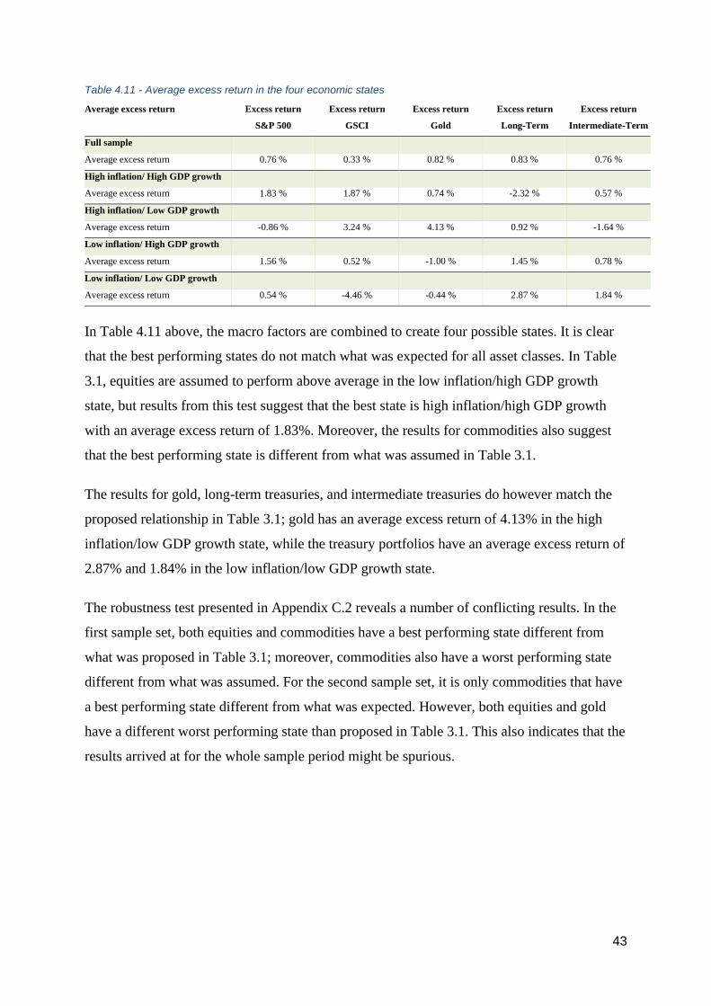
43

Table 4.11 - Average excess return in the four economic states

Average excess return Excess return

S&P 500

Excess return

GSCI

Excess return

Gold

Excess return

Long-Term

Excess return

Intermediate-Term

Full sample

Average excess return 0.76 % 0.33 % 0.82 % 0.83 % 0.76 %


Average excess return 1.83 % 1.87 % 0.74 % -2.32 % 0.57 %


Average excess return -0.86 % 3.24 % 4.13 % 0.92 % -1.64 %


Average excess return 1.56 % 0.52 % -1.00 % 1.45 % 0.78 %


Average excess return 0.54 % -4.46 % -0.44 % 2.87 % 1.84 %

In Table 4.11 above, the macro factors are combined to create four possible states. It is clear

that the best performing states do not match what was expected for all asset classes. In Table

3.1, equities are assumed to perform above average in the low inflation/high GDP growth

state, but results from this test suggest that the best state is high inflation/high GDP growth

with an average excess return of 1.83%. Moreover, the results for commodities also suggest

that the best performing state is different from what was assumed in Table 3.1.

The results for gold, long-term treasuries, and intermediate treasuries do however match the

proposed relationship in Table 3.1; gold has an average excess return of 4.13% in the high

inflation/low GDP growth state, while the treasury portfolios have an average excess return of

2.87% and 1.84% in the low inflation/low GDP growth state.

The robustness test presented in Appendix C.2 reveals a number of conflicting results. In the

first sample set, both equities and commodities have a best performing state different from

what was proposed in Table 3.1; moreover, commodities also have a worst performing state

different from what was assumed. For the second sample set, it is only commodities that have

a best performing state different from what was expected. However, both equities and gold

have a different worst performing state than proposed in Table 3.1. This also indicates that the

results arrived at for the whole sample period might be spurious.

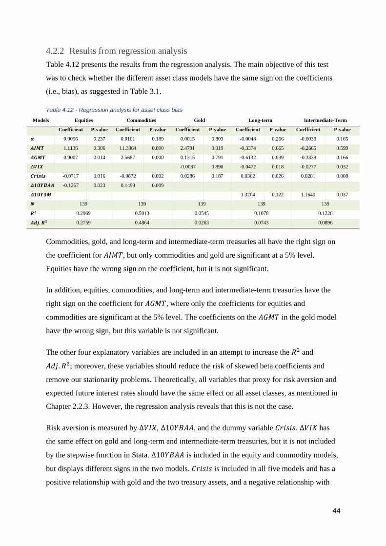
44

4.2.2 Results from regression analysis

Table 4.12 presents the results from the regression analysis. The main objective of this test

was to check whether the different asset class models have the same sign on the coefficients

(i.e., bias), as suggested in Table 3.1.

Table 4.12 - Regression analysis for asset class bias

Models Equities Commodities Gold Long-term Intermediate-Term

Coefficient P-value Coefficient P-value Coefficient P-value Coefficient P-value Coefficient P-value

𝜶 0.0056 0.237 0.0101 0.189 0.0015 0.803 -0.0048 0.266 -0.0039 0.165

𝑨𝑰𝑴𝑻 1.1136 0.306 11.3064 0.000 2.4791 0.019 -0.3374 0.665 -0.2665 0.599

𝑨𝑮𝑴𝑻 0.9007 0.014 2.5687 0.000 0.1315 0.791 -0.6132 0.099 -0.3339 0.166

𝜟𝑽𝑰𝑿 -0.0037 0.890 -0.0472 0.018 -0.0277 0.032

𝑪𝒓𝒊𝒔𝒊𝒔 -0.0717 0.016 -0.0872 0.002 0.0286 0.187 0.0362 0.026 0.0281 0.008

𝜟𝟏𝟎𝒀𝑩𝑨𝑨 -0.1267 0.023 0.1499 0.009

𝜟𝟏𝟎𝒀𝟑𝑴 1.3204 0.122 1.1640 0.037

𝑵 139 139 139 139 139

𝑹𝟐 0.2969 0.5013 0.0545 0.1078 0.1226

𝑨𝒅𝒋. 𝑹𝟐 0.2759 0.4864 0.0263 0.0743 0.0896

Commodities, gold, and long-term and intermediate-term treasuries all have the right sign on

the coefficient for 𝐴𝐼𝑀𝑇, but only commodities and gold are significant at a 5% level.

Equities have the wrong sign on the coefficient, but it is not significant.

In addition, equities, commodities, and long-term and intermediate-term treasuries have the

right sign on the coefficient for 𝐴𝐺𝑀𝑇, where only the coefficients for equities and

commodities are significant at the 5% level. The coefficients on the 𝐴𝐺𝑀𝑇 in the gold model

have the wrong sign, but this variable is not significant.

The other four explanatory variables are included in an attempt to increase the 𝑅2 and

𝐴𝑑𝑗. 𝑅2; moreover, these variables should reduce the risk of skewed beta coefficients and

remove our stationarity problems. Theoretically, all variables that proxy for risk aversion and

expected future interest rates should have the same effect on all asset classes, as mentioned in

Chapter 2.2.3. However, the regression analysis reveals that this is not the case.

Risk aversion is measured by Δ𝑉𝐼𝑋, Δ10𝑌𝐵𝐴𝐴, and the dummy variable 𝐶𝑟𝑖𝑠𝑖𝑠. Δ𝑉𝐼𝑋 has

the same effect on gold and long-term and intermediate-term treasuries, but it is not included

by the stepwise function in Stata. Δ10𝑌𝐵𝐴𝐴 is included in the equity and commodity models,

but displays different signs in the two models. 𝐶𝑟𝑖𝑠𝑖𝑠 is included in all five models and has a

positive relationship with gold and the two treasury assets, and a negative relationship with

45

equities and commodities. Since 𝐶𝑟𝑖𝑠𝑖𝑠 is included in all five models, and has a positive

coefficient in three models and a negative coefficient in two, this indicates that the bias

towards increased risk in the market has a different effect on different asset classes. This

indicates that the theory presented in Chapter 2.2.3 about the drivers of volatility, is not

correct for our sample period. Thus, implying that the risk-aversion factor can be

diversifiable. Δ10𝑌3𝑀 is used as a proxy for the expected interest rate level. This variable

was only included in the two treasury assets, and it is therefore not possible to measure

whether it has another effect on other types of assets.

The above results indicate that the relationship between asset classes and macroeconomic

environments is not as proposed in Bridgewater’s theory. The regression analysis reveals that

none of the variables with the wrong sign on their coefficients are significant. However, if we

combine the results from Chapters 4.2.1 with the results from our regression analysis it is

clear that there are some differences between the proposed relationships and our results.

In Chapter 4.2.1, equities have the ‘correct’ bias, but when the sample period is split into two

periods of approximately 25 years, inflation has a negative impact on equities in the first

period and a positive impact on equities in the second period. Since the regression analysis is

conducted on the last 35 years, and therefore excludes the 1970s when inflation was at

extremely high levels, this may indicate that inflation needs to be above a certain level before

it has a significantly negative effect on equities.

Gold also has the wrong sign on the coefficient for economic growth. This coefficient is not

significant and one of the reasons for this may be that there are small differences in average

return between periods with high and low GDP growth in the last 25 years, as indicated in

Appendix C.1.

Commodities display a clear result in this regression analysis, but this may also be a spurious

result since it is clear that low GDP growth was better for commodities in the first sub-sample

period. Treasuries do not display any significant result, but since there is the correct bias in all

three tests there may be a relationship.

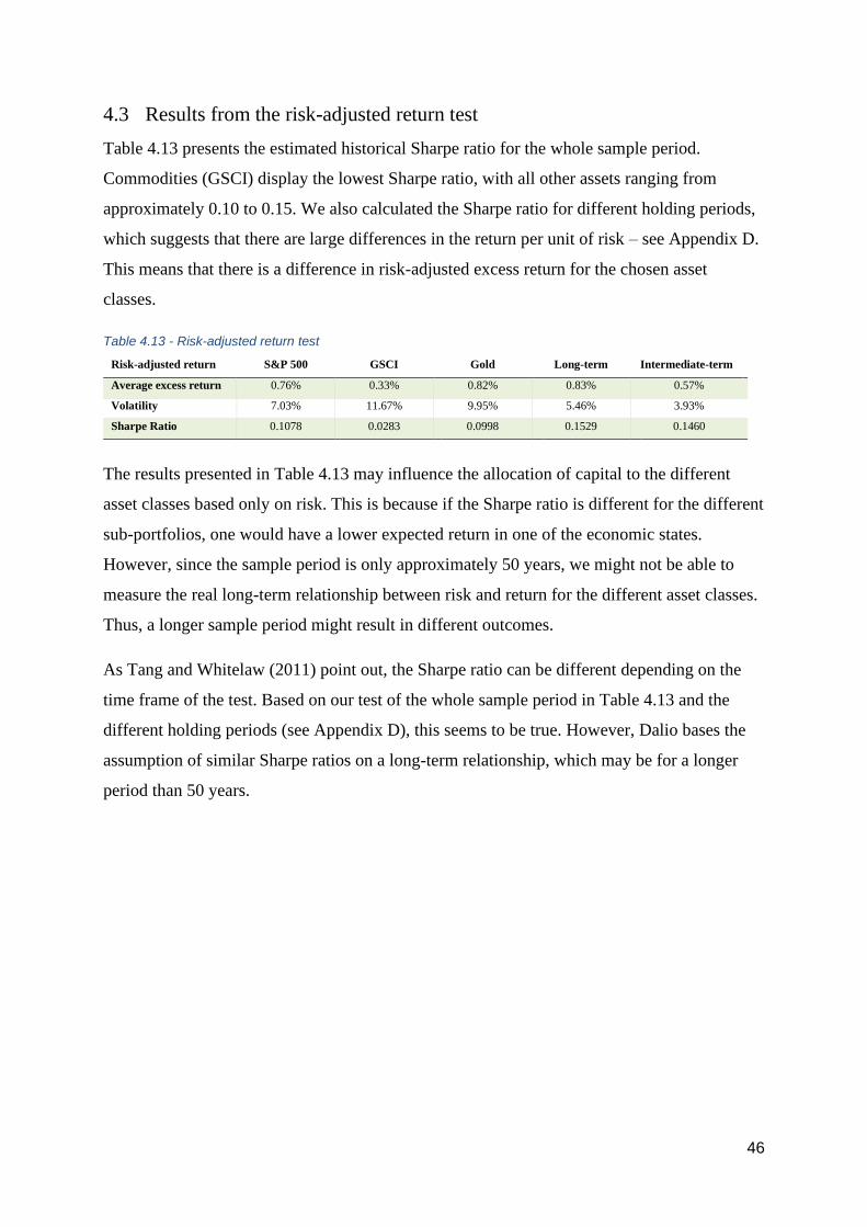
46

4.3 Results from the risk-adjusted return test

Table 4.13 presents the estimated historical Sharpe ratio for the whole sample period.

Commodities (GSCI) display the lowest Sharpe ratio, with all other assets ranging from

approximately 0.10 to 0.15. We also calculated the Sharpe ratio for different holding periods,

which suggests that there are large differences in the return per unit of risk – see Appendix D.

This means that there is a difference in risk-adjusted excess return for the chosen asset

classes.

Table 4.13 - Risk-adjusted return test

Risk-adjusted return S&P 500 GSCI Gold Long-term Intermediate-term

Average excess return 0.76% 0.33% 0.82% 0.83% 0.57%

Volatility 7.03% 11.67% 9.95% 5.46% 3.93%

Sharpe Ratio 0.1078 0.0283 0.0998 0.1529 0.1460

The results presented in Table 4.13 may influence the allocation of capital to the different

asset classes based only on risk. This is because if the Sharpe ratio is different for the different

sub-portfolios, one would have a lower expected return in one of the economic states.

However, since the sample period is only approximately 50 years, we might not be able to

measure the real long-term relationship between risk and return for the different asset classes.

Thus, a longer sample period might result in different outcomes.

As Tang and Whitelaw (2011) point out, the Sharpe ratio can be different depending on the

time frame of the test. Based on our test of the whole sample period in Table 4.13 and the

different holding periods (see Appendix D), this seems to be true. However, Dalio bases the

assumption of similar Sharpe ratios on a long-term relationship, which may be for a longer

period than 50 years.

47

5 Conclusion and further prospects

This thesis has examined the following research question:

How does the all-weather portfolio perform compared to the 60/40 and all-equity portfolios,

and are the assumptions for the all-weather portfolio valid?

We found that the all-weather portfolio provides a higher risk-adjusted return than the 60/40

and all-equity portfolios, and that it has a lower downside risk for the sample period.

However, we cannot confirm that the assumptions made for the construction of the portfolio

are valid.

The results in Chapter 4.1 demonstrate that we can create a portfolio which has a balanced

risk contribution across the four different economic states if the asset classes have the

economic bias as discussed in Chapter 2.2.4. We also found that the all-weather portfolio had

the highest total return of the three portfolios for the whole sample period. Furthermore, the

all-weather portfolio has the second highest average quarterly return for the whole sample

period. However, the portfolio is superior in terms of standard deviation, value at risk, and

conditional value at risk, and it has the highest risk-adjusted return.

In addition, we calculated the average return on rolling holding periods. Here the results

indicated that the all-weather portfolio did not have the highest average or maximum return in

any of the different holding periods. This was also true for the median returns, except for the

20-year holding period. However, the downside risk measurements on the rolling holding

periods indicated that the all-weather portfolio has the highest minimum return in all holding

periods. Value at risk and conditional value at risk are also higher (i.e., less risk) for the all-

weather portfolio, and the percentage of negative returns were lower than or equal to the other

portfolios.

We also tested whether the portfolio has a bias towards an economic state, and if it performed

better or worse than the average return. Here we found that the all-weather portfolio had the

least deviation from the average return, and that the average return in the poorest state was

higher than the worst state of the other portfolios. The all-weather portfolio also had the

lowest maximum and average drawdown, as well as the shortest recovery time.

48

The results indicate that the all-weather portfolio may not provide superior returns; however,

the goal of an all-weather portfolio is not to provide exceptional returns, but rather to increase

the risk-adjusted return and to protect against downside risk. We therefore reject null

hypothesis 1.

The results in Chapter 4.2 demonstrate that the relationship between asset class return and

economic bias/state is inconsistent, and we therefore cannot reject null hypothesis 2.

The average return for the asset classes in periods of either high or low inflation and GDP

growth was as expected when we used the whole sample period. However, when we divided

the sample period into two parts, the biases were no longer the same for both periods. This

result indicates that the relationship is not reliable.

When the macro factors were combined into four states, we found that the assumed best states

according to the theory did not always correspond with the best state identified in the test. It

was observed that both equities and commodities had their best performing economic state in

a state other than the one suggested by the theory. On the other hand, the test indicated that in

the worst economic state, asset classes had below average excess return, which was in line

with the theory. When we divided the sample periods into two parts, the results demonstrated

a different outcome for the combined states, indicating that the relationship between asset

classes and economic states might be spurious.

The results of the regression analysis demonstrate that only the commodity model had

significant coefficients with the expected sign on both 𝐴𝐼𝑀𝑇 and 𝐴𝐺𝑀𝑇. For the equity and

gold model, only one of the risk factor coefficients was found to be significant with the ‘right’

sign; the other was non-significant with the ‘wrong’ sign. The treasury models had no

significant coefficients, but all coefficients had the expected sign.

In Chapter 4.3, the test for risk-adjusted return exhibited a large difference in Sharpe ratio for

the five asset classes. This indicates that risk-adjusted performance is not similar for all asset

classes, at least not in the sample period used in this thesis. We therefore cannot reject null

hypothesis 3. This result has implications for allocating based on risk only. This is because

when one is paid more for exposure to one economic state, in terms of return per unit of risk,

it makes sense to have an overweight in that sub-portfolio.

49

The results regarding economic biases and risk-adjusted returns give rise to two points that

future researchers could investigate. First, we limited ourselves to macroeconomic data from

the U.S., but since commodities, gold, and to a lesser extent the S&P 500 are international

asset classes, inflation and GDP data from other major economies could have been included.

In addition, Bridgewater Associates examined the economical biases and risk-adjusted return

over several centuries, while this thesis analysed data relating to the past 50 years. It would

therefore be interesting to test the economical biases and Sharpe ratio for an even longer time

frame.

50

6 References

Amato, L., & Lohre, H. (2020, August 31). Diversifying Macroeconomic Factors—for Better

or for Worse. SSRN. http://dx.doi.org/10.2139/ssrn.3730154

Ang, Andrew. (2014). Asset Management. Oxford University Press.

https://doi.org/10.1093/acprof:oso/9780199959327.001.0001

Baltas, Nick. (2016). 3 - Trend-Following, Risk-Parity and the Influence of Correlations. In

Risk-Based and Factor Investing (pp. 65–95). Elsevier Ltd. https://doi.org/10.1016/B978-1-

78548-008-9.50003-4

Barucci, Emilio, & Fontana, Claudio. (2017). Financial Markets Microstructure. In Financial

Markets Theory (pp. 583–659). Springer London. https://doi.org/10.1007/978-1-4471-7322-

9_10

Bhansali, Vineer. (2011). Beyond Risk Parity. The Journal of Investing, 20(1), 137–147.

https://doi.org/10.3905/joi.2011.20.1.137

Bhansali, Vineer, Davis, Josh, Rennison, Graham, Hsu, Jason, & Li, Feifei. (2012). The Risk

in Risk Parity: A Factor-Based Analysis of Asset-Based Risk Parity. The Journal of Investing,

21(3), 102–110. https://doi.org/10.3905/joi.2012.21.3.102

Blanchard, Olivier. (2019). Public Debt and Low Interest Rates. The American Economic

Review, 109(4), 1197–1229. https://doi.org/10.1257/aer.109.4.1197

Bridgewater Associates. (2012, January). The All Weather Story, Bridgewater.

https://www.bridgewater.com/research-and-insights/the-all-weather-story

Bruder, B., & Roncalli, T. (2012, January 20). Managing risk exposures using the risk

budgeting approach. SSRN. http://dx.doi.org/10.2139/ssrn.2009778

Carhart, Mark M. (1997). On Persistence in Mutual Fund Performance. The Journal of

Finance (New York), 52(1), 57–82. https://doi.org/10.1111/j.1540-6261.1997.tb03808.x

Chaves, Denis, Hsu, Jason, Li, Feifei, & Shakernia, Omid. (2012). Efficient Algorithms for

Computing Risk Parity Portfolio Weights. The Journal of Investing, 21(3), 150–163.

https://doi.org/10.3905/joi.2012.21.3.150

Congressional Research Service. (2021, January). Introduction to U.S. Economy: The

Business Cycle and Growth. Fas. https://fas.org/sgp/crs/misc/IF10411.pdf

Coudert, Virginie, & Gex, Mathieu. (2008). Does risk aversion drive financial crises? Testing

the predictive power of empirical indicators. Journal of Empirical Finance, 15(2), 167–184.

https://doi.org/10.1016/j.jempfin.2007.06.001

Dalio, Ray. (2004). Engineering targeted returns and risks: Ray Dalio, founder of Bridgewater

Associates, explains how to achieve a 10% return by taking 10% to 12% risk. Global

Investor, 178, 58.

51

Dalio, R. (2012). How the economic machine works. Academia. Retrieved March 06, 2021,

from

https://www.academia.edu/3802715/How_the_Economic_Machine_Works_A_Template_for_

Understanding_What_is_Happening_Now_Ray_Dalio_Bridgewater

Dempster, Natalie, & Artigas, Juan Carlos. (2010). Gold: Inflation hedge and long-term

strategic asset. The Journal of Wealth Management, 13(2), 69–75.

https://doi.org/10.3905/jwm.2010.13.2.069

Fama, Eugene F, & French, Kenneth R. (1996). Multifactor Explanations of Asset Pricing

Anomalies. The Journal of Finance (New York), 51(1), 55–84. https://doi.org/10.1111/j.1540-

6261.1996.tb05202.x

Fan, Wei, Fang, Sihai, & Lu, Tao. (2014). Macro-factors on gold pricing during the financial

crisis. China Finance Review International, 4(1), 58–75. https://doi.org/10.1108/CFRI-09-

2012-0097

Finra. U.S. Treasury Securities. Retrieved March 10, 2021, from

https://www.finra.org/investors/learn-to-invest/types-investments/bonds/types-of-bonds/us-

treasury-securities

Greer, RJ. (1997). What is an asset class, anyway? Journal of Portfolio Management, 23(2),

86–91. https://doi.org/10.3905/jpm.23.2.86

Gupta, Rangan, Subramaniam, Sowmya, Bouri, Elie, & Ji, Qiang. (2021). Infectious disease-

related uncertainty and the safe-haven characteristic of US treasury securities. International

Review of Economics & Finance, 71, 289–298. https://doi.org/10.1016/j.iref.2020.09.019

Hendricks, Darryll. (1996). Evaluation of value-at-risk models using historical data.

Economic Policy Review (Federal Reserve Bank of New York), 2(1), 39.

Ilmanen, Antti, Maloney, Thomas, & Ross, Adrienne. (2014). Exploring macroeconomic

sensitivities: How investments respond to different economic environments. Journal of

Portfolio Management, 40(3), 87–99. https://doi.org/10.3905/jpm.2014.40.3.087

Jensen, G., & Rotenberg, J. (2004, August 18). The biggest mistake in investing. Bridgewater.

https://www.bridgewater.com/research-and-insights/the-biggest-mistake-in-investing

Leite, André Luis, Klotzle, Marcelo Cabus, Pinto, Antonio Carlos Figueiredo, & da Silveira

Barbedo, Claudio Henrique. (2020). The Fama-French’s five-factor model relation with

interest rates and macro variables. The North American Journal of Economics and Finance,

53, 101197. https://doi.org/10.1016/j.najef.2020.101197

Lian, Chen, Ma, Yueran, & Wang, Carmen. (2019). Low Interest Rates and Risk-Taking:

Evidence from Individual Investment Decisions. The Review of Financial Studies, 32(6),

2107–2148. https://doi.org/10.1093/rfs/hhy111

Lintner, John. (1965). The Valuation of Risk Assets and the Selection of Risky Investments in

Stock Portfolios and Capital Budgets. The Review of Economics and Statistics, 47(1), 13–37.

https://doi.org/10.2307/1924119

Markowitz, H. (1952). Portfolio selection. Journal of finance, 7(1), 77-91.

52

Markowitz, HM. (1991). FOUNDATIONS OF PORTFOLIO THEORY. The Journal of

Finance (New York), 46(2), 469–477. https://doi.org/10.2307/2328831

Martellini, Lionel, Milhau, Vincent, & Tarelli, Andrea. (2015). Toward conditional risk

parity: Improving risk budgeting techniques in changing economic environments. The Journal

of Alternative Investments, 18(1), 48–64. https://doi.org/10.3905/jai.2015.18.1.048

Mokkelbost, Per B. (1971). Unsystematic Risk Over Time. Journal of Financial and

Quantitative Analysis, 6(2), 785–796. https://doi.org/10.2307/2329714

Mossin, Jan. (1966). Equilibrium in a Capital Asset Market. Econometrica, 34(4), 768–783.

https://doi.org/10.2307/1910098

Nai-Fu Chen, Richard Roll, & Stephen A. Ross. (1986). Economic Forces and the Stock

Market. The Journal of Business (Chicago, Ill.), 59(3), 383–403.

https://doi.org/10.1086/296344

Neill Fortune, J. (1987). The inflation rate of the price of gold, expected prices and interest

rates. Journal of Macroeconomics, 9(1), 71–82. https://doi.org/10.1016/S0164-

0704(87)80007-1

O'Connor, Fergal A, Lucey, Brian M, Batten, Jonathan A, & Baur, Dirk G. (2015). The

financial economics of gold — A survey. International Review of Financial Analysis, 41,

186–205. https://doi.org/10.1016/j.irfa.2015.07.005

Page, Sébastien, & Taborsky, Mark A. (2011). The myth of diversification: Risk factors

versus asset classes. Journal of Portfolio Management, 37(4), 1–2.

https://doi.org/10.3905/jpm.2011.37.4.001

Pastor, L, & Stambaugh, RF. (2003). Liquidity Risk and Expected Stock Returns. The Journal

of Political Economy, 111(3), 642–685. https://doi.org/10.1086/374184

Prince, B. (2011, August). Risk Parity Is About Balance. Bridgewater.

https://www.bridgewater.com/research-and-insights/risk-parity-is-about-balance

Qian, Edward. (2011). Risk Parity and Diversification. The Journal of Investing, 20(1), 119–

127. https://doi.org/10.3905/joi.2011.20.1.119

Roache, Shaun K, & Rossi, Marco. (2010). The effects of economic news on commodity

prices. The Quarterly Review of Economics and Finance, 50(3), 377–385.

https://doi.org/10.1016/j.qref.2010.02.007

Robbins, T. (2014). Money master the game: 7 simple steps to financial freedom. Simon and

Schuster.

Ross, Stephen A. (1976). The arbitrage theory of capital asset pricing. Journal of Economic

Theory, 13(3), 341–360. https://doi.org/10.1016/0022-0531(76)90046-6

Shahidi, A. (2014). Balanced asset allocation: how to profit in any economic climate. John

Wiley & Sons, Inc.

53

Sharpe, William F. (1964). Capital Asset Prices: A Theory of Market Equilibrium under

Conditions of Risk. The Journal of Finance (New York), 19(3), 425–442.

https://doi.org/10.1111/j.1540-6261.1964.tb02865.x

Sharpe, W. F. (1994). The sharpe ratio. Journal of portfolio management, 21(1), 49-58.

Stoll, Hans R, & Whaley, Robert E. (2010). Commodity index investing and commodity

futures prices. Journal of Applied Finance: JAF, 20(1), 7.

Studenmund, A. H., & Johnson, B. K. (2017). A Practical guide to using econometrics (7th

edition, global edition.). Pearson.

Swinkels, L. (2019, June 28). Treasury bond return data starting in 1962. MDPI.

https://doi.org/10.3390/data4030091

Szegö, Giorgio. (2002). Measures of risk. Journal of Banking & Finance, 26(7), 1253–1272.

https://doi.org/10.1016/S0378-4266(02)00262-5

Tang, Y., & Whitelaw, R. F. (2011). Time-varying Sharpe ratios and market timing. The

Quarterly Journal of Finance, 1(03), 465-493. https://doi.org/10.1142/S2010139211000122

Thomas, R. L. (2005). Using statistics in economics (pp. XIV, 611). McGraw Hill.

U.S. Department of the treasury. (2021, May 20). Daily Treasury Yield Curve Rates.

Treasury.gov. https://www.treasury.gov/resource-center/data-chart-center/interest-

rates/Pages/TextView.aspx?data=yieldAll

54

Appendices

Appendix A: Descriptive statistics

A.1 Historical price development for the five asset classes used in this thesis, this is from

01.04.1970 to 01.01.2021

A.2 Descriptive statistics for the five asset classes from 01.04.1970 to 01.01.2021

A.3 Quarterly return distribution for the five asset classes

Descriptive statistics Mean St.dev Max Min Skewness Kurtosis

S&P 500 0.0221 0.0702 0.2221 -0.2687 -0.9209 5.6316

GSCI 0.0076 0.1166 0.2976 -0.5378 -1.6535 8.8913

Gold 0.0102 0.0680 0.2241 -0.1466 0.3611 3.2839

Long-term 0.0224 0.0529 0.2013 -0.0940 0.7402 3.9613

Intermediate-term 0.0181 0.0365 0.1613 -0.0523 0.7920 3.9365

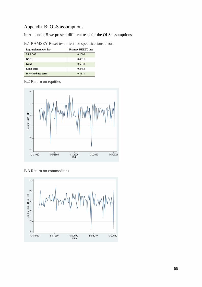
55

Appendix B: OLS assumptions

In Appendix B we present different tests for the OLS assumptions

B.1 RAMSEY Reset test – test for specifications error.

B.2 Return on equities

B.3 Return on commodities

Regression model for: Ramsey RESET test

S&P 500 0.1506

GSCI 0.4311

Gold 0.6018

Long-term 0.2453

Intermediate-term 0.3811

56

B.4 Return on gold

B.5 Return on long-term treasuries

B.6 Return on intermediate-term treasuries

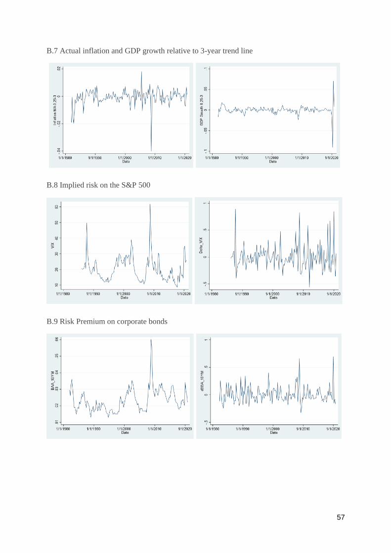
57

B.7 Actual inflation and GDP growth relative to 3-year trend line

B.8 Implied risk on the S&P 500

B.9 Risk Premium on corporate bonds

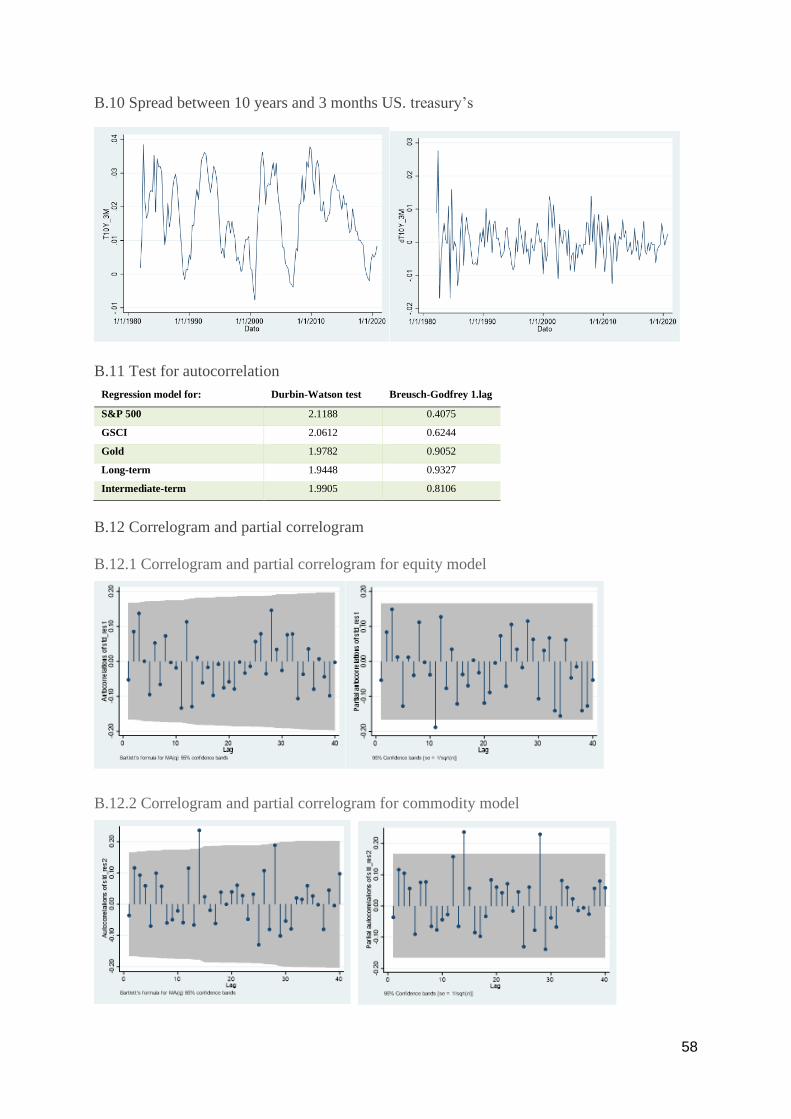
58

B.10 Spread between 10 years and 3 months US. treasury’s

B.11 Test for autocorrelation

B.12 Correlogram and partial correlogram

B.12.1 Correlogram and partial correlogram for equity model

B.12.2 Correlogram and partial correlogram for commodity model

Regression model for: Durbin-Watson test Breusch-Godfrey 1.lag

S&P 500 2.1188 0.4075

GSCI 2.0612 0.6244

Gold 1.9782 0.9052

Long-term 1.9448 0.9327

Intermediate-term 1.9905 0.8106

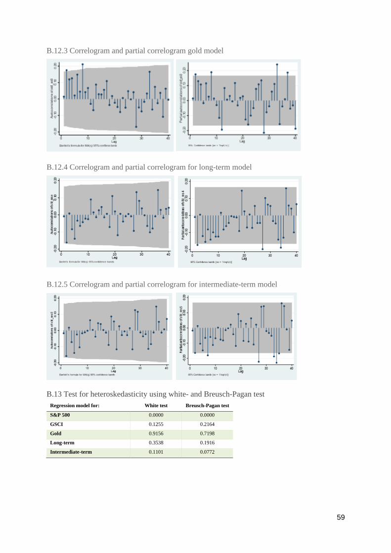
59

B.12.3 Correlogram and partial correlogram gold model

B.12.4 Correlogram and partial correlogram for long-term model

B.12.5 Correlogram and partial correlogram for intermediate-term model

B.13 Test for heteroskedasticity using white- and Breusch-Pagan test

Regression model for: White test Breusch-Pagan test

S&P 500 0.0000 0.0000

GSCI 0.1255 0.2164

Gold 0.9156 0.7198

Long-term 0.3538 0.1916

Intermediate-term 0.1101 0.0772

60

B.14 Correlation matrix for the independent variables

B.15 Test for multicollinearity using VIF

B.16 Test for normality

Correlation: 1 2 3 4 5 6

𝑨𝑰𝑴𝑻 1.000

𝑨𝑮𝑴𝑻 0.269 1.000

𝚫𝑽𝑰𝑿 -0.315 -0.194 1.000

𝑪𝒓𝒊𝒔𝒊𝒔 -0.185 -0.316 0.313 1.000

𝜟𝟏𝟎𝒀𝑩𝑨𝑨 -0.319 -0.170 0,552 0.211 1.000

𝜟𝑻𝟏𝟎𝟑𝑴 0.1087 0.000 -0.112 -0.087 -0.243 1.000

Regression model for: VIF-Test

S&P 500 1.16

GSCI 1.16

Gold 1.19

Long-term 1.16

Intermediate-term 1.16

Regression model

for:

Skewness and kurtosis

tests for normality

pr(skewness)

Skewness and kurtosis

tests for normality

p(kurtosis)

Shapiro-Wilk W test for

normal data

Shapiro-Francia W' test

for normal data

S&P 500 0.3810 0.0086 0.02585 0.00911

GSCI 0.0467 0.0030 0.00289 0.00161

Gold 0.1155 0.9629 0.41312 0.45330

Long-term 0.1876 0.1076 0.31496 0.15876

Intermediate-term 0.6746 0.5747 0.90720 0.97864

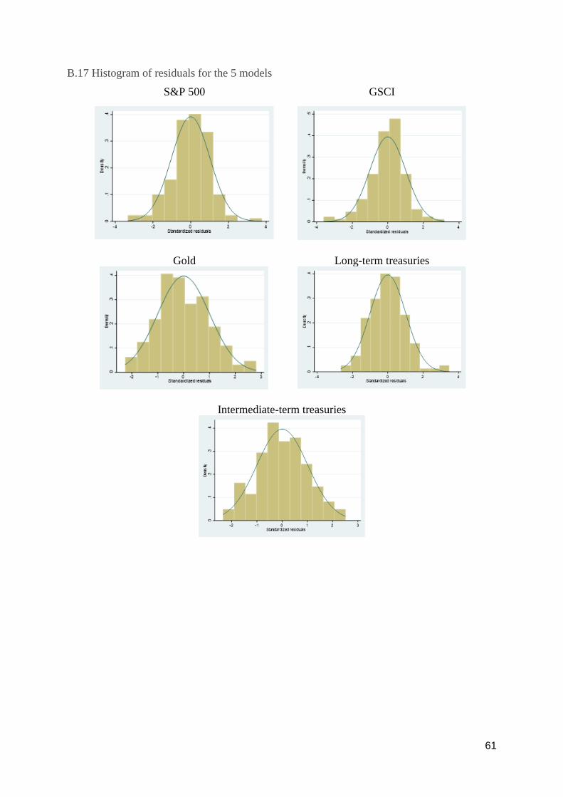
61

B.17 Histogram of residuals for the 5 models

S&P 500 GSCI

Gold

Long-term treasuries

Intermediate-term treasuries

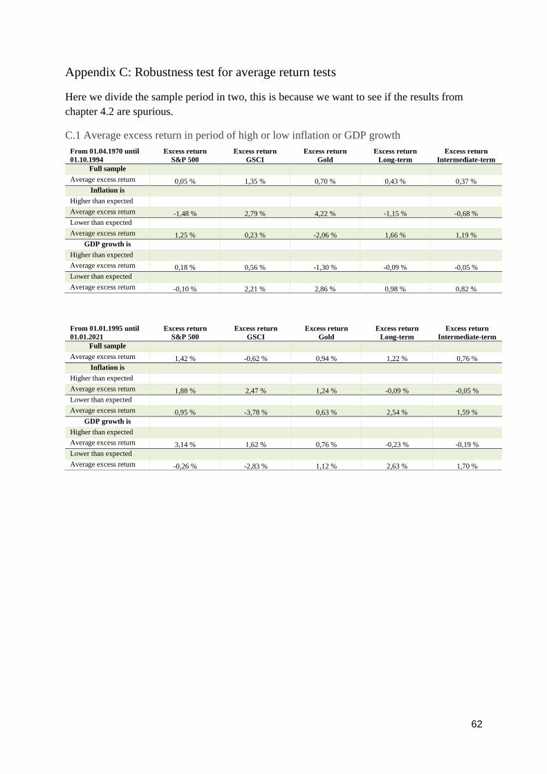
62

Appendix C: Robustness test for average return tests

Here we divide the sample period in two, this is because we want to see if the results from

chapter 4.2 are spurious.

C.1 Average excess return in period of high or low inflation or GDP growth

From 01.04.1970 until

01.10.1994

Excess return

S&P 500

Excess return

GSCI

Excess return

Gold

Excess return

Long-term

Excess return

Intermediate-term

Full sample

Average excess return 0,05 % 1,35 % 0,70 % 0,43 % 0,37 %

Inflation is


Average excess return -1,48 % 2,79 % 4,22 % -1,15 % -0,68 %

Lower than expected

Average excess return 1,25 % 0,23 % -2,06 % 1,66 % 1,19 %

GDP growth is


Average excess return 0,18 % 0,56 % -1,30 % -0,09 % -0,05 %

Lower than expected

Average excess return -0,10 % 2,21 % 2,86 % 0,98 % 0,82 %

From 01.01.1995 until

01.01.2021

Excess return

S&P 500

Excess return

GSCI

Excess return

Gold

Excess return

Long-term

Excess return

Intermediate-term

Full sample

Average excess return 1,42 % -0,62 % 0,94 % 1,22 % 0,76 %

Inflation is


Average excess return 1,88 % 2,47 % 1,24 % -0,09 % -0,05 %

Lower than expected


GDP growth is



Lower than expected

Average excess return -0,26 % -2,83 % 1,12 % 2,63 % 1,70 %

63

C.2 Average excess return in period of combinations of high/high, high/low, low/high, and

low/low inflation or GDP growth

From 01.04.1970 until 01.10.1994 Excess return

S&P 500

Excess return

GSCI

Excess return

Gold

Excess return

Long-term

Excess return

Intermediate-term

Full sample



Average excess return -0,45 % 1,61 % 0,71 % -3,41 % -2,56 %


Average excess return -1,98 % 3,36 % 5,92 % -0,06 % 0,22 %





From 01.01.1995 until 01.01.2021 Excess return

S&P 500

Excess return

GSCI

Excess return

Gold

Excess return

Long-term

Excess return

Intermediate-term

Full sample









Average excess return -0,89 % -7,36 % 0,54 % 3,00 % 1,87 %

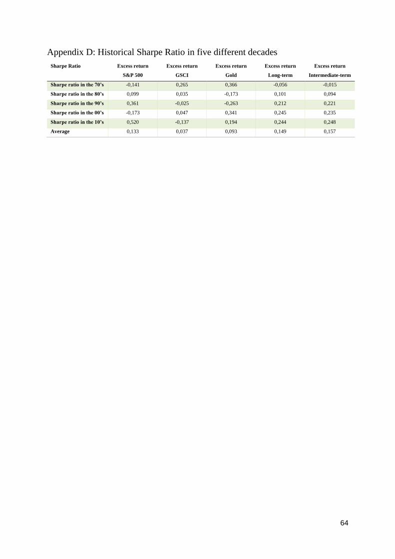
64

Appendix D: Historical Sharpe Ratio in five different decades

Sharpe Ratio Excess return

S&P 500

Excess return

GSCI

Excess return

Gold

Excess return

Long-term

Excess return

Intermediate-term

Sharpe ratio in the 70’s -0,141 0,265 0,366 -0,056 -0,015

Sharpe ratio in the 80’s 0,099 0,035 -0,173 0,101 0,094

Sharpe ratio in the 90’s 0,361 -0,025 -0,263 0,212 0,221

Sharpe ratio in the 00’s -0,173 0,047 0,341 0,245 0,235

Sharpe ratio in the 10’s 0,520 -0,137 0,194 0,244 0,248

Average 0,133 0,037 0,093 0,149 0,157

NTN

UN

orw

egia

n U

nive

rsity

of S

cien

ce a

nd T

echn

olog

yFa

culty

of E

cono

mic

s an

d M

anag

emen

t N

TNU

Bus

ines

s Sc

hool




Master’s thesis in Economics and Business AdministrationSupervisor: Denis M. Becker

May 2021

Mas

ter’s

thes

is

Documents

The all-weather portfolio - NTNU Open