Embed Size (px)
Citation preview

Testing Distributed Systems through SymbolicModel Checking of Traces
Gabriel Kalyon?, Thierry Massart, Cedric Meuter, and Laurent Van Begin??
Universite Libre de Bruxelles (U.L.B.),Boulevard du Triomphe, CP-212, 1050 Bruxelles, BELGIUM
{gkalyon,tmassart,cmeuter,lvbegin}@ulb.ac.be
Abstract. The observation of a distributed system’s finite execution canbe abstracted as a partial ordered set of events generally called finite trace.In practice, this trace can be obtained through a standard code instru-mentation, which takes advantage of existing communications betweenprocesses to partially order events of different processes. We show thattesting that such a distributed execution satisfies some global propertyamounts therefore to model check the corresponding trace. This work canbe time consuming; we therefore provide an efficient symbolic Ctl model-checking algorithm for traces. This method is based on a symbolic datastructure, called Interval Sharing Trees, allowing to efficiently representand manipulate sets of k-uples of naturals. Efficient symbolic operationsare defined on this data structure in order to deal with all Ctl modali-ties. We show that in practice this data structure is well adapted for Ctlmodel checking of traces.
Keywords: testing, asynchronous distributed systems, global property,model checking of traces, trace checking
1 Introduction
A distributed system is typically a set of distributed hardware equipments whichrun concurrent processes, communicating through some network. The design ofsuch system is known to be a difficult task. When the purpose of such a system isto perform some control of critical equipment like an industrial plant, a plane, ora satellite, its correctness is extremely important. The designer can ease her workby various techniques [1, 2] including validation and debugging. In particular,traditional model-based approaches abstract the action the system can do intoevents which change the system’s global state. Validation works therefore on alabelled directed graph called a Kripke structure which describes the possiblesystem’s behaviours. Verification tools (e.g. [3–5]) can be used to validate parts ofmodels. For instance, such tools can be used to check that, in the system, everytime the system goes in a state where a condition p holds, it is followed by astate where q and r holds. p can for instance be an abstraction for some alarmdetected through some given sensor, while q and r, may correspond to, possiblydistributed, values assignment on some actuators.? Supported by the Belgian National Science Foundation (FNRS) under a FRIA grant.
?? Research fellow supported by the Belgian National Science Foundation (FNRS).

2 Gabriel Kalyon, Thierry Massart, Cedric Meuter, and Laurent Van Begin
Unfortunately in practice, even with this abstraction, the state-explosion prob-lem generally prevents the designer from exhaustively verifying the whole system,even with efficient exploration techniques such as partial order reduction [6, 7] orsymbolic model checking [8–10].
In such cases, the designer generally falls back to testing which cannot guar-antee that a system is completely bug-free, but if achieved on a large numberof test-cases (e.g. covering all the functionalities of the system), can give a rea-sonable confidence that the system is correct. In this context, a test-case definesthe model of the part of the system which corresponds to a particular execution.Testing may therefore be seen as the validation of this smaller model.
To extract this smaller model from a system, the implementation is instru-mented to record only relevant events. A special process, called the monitor,records this model (the events of the system), that we can just call executionhere, and then checks that it satisfies some desired property.
Notice that an execution can also be extracted from a design model. In par-ticular scenarios of executions, modelled as MSC (Message Sequence Charts) is aparticular form of such execution and can also be validated. Hence, at both thedesign and implementation levels, it is an important activity for which efficientmethods must be provided.
In the centralized case, an execution of the system is a sequence of events.Determining if such an execution satisfies a property is in general simple. Inthe distributed case, if the system to control is slow enough, one can assumethat all processes of the system are synchronized using a global discrete clock.This so-called synchrony hypothesis allows to see such distributed execution as asequence of set of events where all events in a set are seen as simultaneous. Thishypothesis allows a relatively simple validation of such a distributed execution.Unfortunately, if the system to control is too fast compared to the synchronizationmechanism offered by the implementation, the synchrony hypothesis cannot bemade and the asynchronism between distributed processes must be taken intoaccount in the analysis. In this case, the exact order in which two concurrentevents occur in the execution is, in general, not always known or guaranteed. Bytaking into account the communications between processes, only a partial orderon the events of the execution can be obtained. In practice, this partial orderrelation, often called the happened-before relation [11], can be obtained throughcorrect code instrumentation using, for instance, vector clocks [11, 12].
Hence in this case, an execution is a finite trace, i.e. a partially ordered set ofevents. Since the order in which the events of this partial order trace are inter-leaved is generally relevant to the safety of the system, testing that a distributedexecution satisfies a global property φ amounts to verifying that every sequentialexecution, compatible with the partial order, satisfies φ or, in other terms, modelchecking φ on the corresponding trace. Unfortunately, this problem is hard [13],since the number of compatible sequential executions and the size of the Kripkestructure which models an execution may be exponential in the number of con-current processes. Therefore, to tackle this complexity, instead of working on theunderlying Kripke structure, efficient techniques have been developed to workdirectly on the partial order itself, which is, in general, exponentially more com-

Testing Distributed Systems through Symbolic Model Checking of Traces 3
pact. In this line, in [14], A. Sen and Garg present the temporal logic RCtl (forregular-Ctl), which is a subset of the branching time temporal logic Ctl [15] andshows that the compact symbolic data structure called computation slice [16], canbe used to efficiently compute all global states which satisfy a RCtl formula.
However, RCtl does not include such simple Ctl property as AG(p =⇒AF(q ∧ r)), i.e. every p is eventually followed by a state where q and r hold true;formula that may be very useful during validation. In general, a computation sliceis too restrictive to represent any arbitrary set of global states of a finite trace.
This motivates our work; in this paper, we introduce an efficient symbolicmethod using Interval Sharing Trees (IST) [17, 18]. This data structure allowsto represent any set of global states of a finite trace. We define how to use ISTto provide a full Ctl model checking of finite traces. We show that intervals ofnaturals can be used, in practice, to have a compact representation for sets ofglobal states of the trace satisfying the desired formula and hence, to provide anefficient algorithm for Ctl model checking of finite traces. Moreover, we show thatour algorithms perform very well compared to standard symbolic model checkingusing BDDs [10] and implemented in the tool NuSMV [5].
This paper is organized as follows. In section 2, we detail related works. Insection 3, we introduce our model for traces and define the Ctl over this model.In section 4, we explain how sets of configurations can be represented compactlyusing intervals and interval sharing trees. In section 5, we show how Ctl modelchecking on traces can be solved using this symbolic representation. Next, insection 6, we experimentally validate our method on various examples comparedto Ctl model-checking with the NuSMV tool. Finally, future works are given insection 7. Note : all proofs from sec. 5 are included for the reviewers in app. A.
2 Related Works
Testing and monitoring the global behaviours of distributed systems can be cat-egorized in two classes: trace model-checking and global predicate detection.
Trace model checking has been studied mainly theoretically through the def-inition of several linear temporal logic for Mazurkiewicz traces. A Mazurkiewicztrace [19], over an alphabet Σ with a independence relation I, can be definedas a Σ-labelled partial order set of events with special properties not explainedhere. For Mazurkiewicz traces, local [20, 21] and global [22–24] trace logics havebeen defined. However, in our case, the trace is an abstraction of a distributedexecution (or of a scenario) and models a set of possible interleaving of eventsthe distributed system may have had. Since we do not suppose to have informa-tion about independence between actions, none of these actions are independenta priori; testing must then check that all these possible orderings of events arecorrect. Since the independence relation is not a data that trace temporal logicsmay exploit, we do not use these logics to model-check our executions and stickto simple sequence (interleaving) semantics.
Global predicate detection initially aims at answering reachability questions,i.e. does there exist a possible global configuration of the system, that satisfiesa given global predicate φ. Garg and Chase showed in [13] that this problem is

4 Gabriel Kalyon, Thierry Massart, Cedric Meuter, and Laurent Van Begin
NP-complete for an arbitrary predicate, even when there is no inter-process com-munication. Efficient (polynomial) methods have been proposed for various classesof predicates, such as stable predicates proposed by Chandy and Lamport [25],independent predicates by Charron-Bost et al [26], conjunctive predicates by Gargand Waldecker [27, 28], linear and semi-linear predicates by Chase and Garg [13],regular predicates by Garg and Mittal [29] and predicates expressed by a finiteautomata that can be checked online by Jard et al [30]. Garg and Mittal implicitlyuse a symbolic data structure called computation slice, to compute efficiently allglobal states, compatible with a given execution satisfying a given regular predi-cate [16]. This structure in used by A. Sen and Garg in their work on the temporallogic RCtl [14]. In [31, 32] K. Sen et al. use an automaton to specify the system’smonitor. The authors provide an explicit exploration of the state space and tolimit this exploration a window is used. In a previous work [33], we have used thistechnique to provide an efficient Ltl tester of distributed executions.
3 Framework
In this section, we detail our framework. We start by formally introducing ourmodel for traces of distributed systems, i.e. finite partial order trace. Then, wedefine the branching time temporal logic Ctl over such finite traces.
3.1 Partial Order Trace
Our executions are obtained by a fixed numbers of concurrent processes, eachexecuting a finite sequence of assignments. Moreover, due to inter-process com-munications (shared variable, message passing, ...), other causal dependencies areadded. An execution is modeled as a finite partial order trace, i.e. a finite partiallyordered set of events, where each event belongs to some process and is labeled bythe assignment which took place during this event.
Definition 1 (Partial order trace). A partial order trace of k processes andover a set of variables V is a tuple T = 〈E,α,�〉 where:
– E = P1 ∪ P2 ∪ ... ∪ Pk is a finite set of events partitioned into k disjointnon empty subsets Pi, called processes; pid(e) denotes the process of event ebelongs to (pid(e) = i iff e ∈ Pi);
– α : E 7→ V × Q is a labeling function mapping each event to an assignment,i.e. α(e) = (x, v) associates the assignment x := v to e; if α(e) = (x := v),var(e) denotes x and val(e) denotes v;
– �⊆ E × E is a partial order relation on E such that ∀e, e′ ∈ E:(i) pid(e) = pid(e′) ⇒ (e � e′) ∨ (e′ � e)(ii) var(e) = var(e′) ⇒ (e � e′) ∨ (e′ � e).
Condition (i) on � ensures that all events from the same process are orderedand condition (ii) enforces that all events assigning the same variable are ordered.Given an event e ∈ E, we define ↓e = {e′ ∈ E | e′ � e}, the past of e (includingitself), and pos(e) = |↓e∩Ppid(e)| (where | · | denotes the size of sets), the position

Testing Distributed Systems through Symbolic Model Checking of Traces 5
P1 w:=1 y:=3 x:=0
P2 x:=4 w:=0
Fig. 1. Example of partial order trace
of e in its process. A cut is a subset C ⊆ E such that ∀e ∈ C :↓e ⊆ C. cuts(T) ={C ⊆ E | ∀e ∈ C : ↓e ⊆ C} is the set of all cuts in T. In the remainder of thispaper, we always consider the set of variables V and the partial order trace of kprocesses T = 〈E,α,�〉.
Semantics. Given a cut C ∈ cuts(T), we define enabled(C) = {e ∈ E \ C | (↓e \ {e}) ⊆ C} the set of events enabled in C. If e is enabled in the cut C, thenit can be fired from C leading to C ∪ {e}, the successor of C for e. Note that ifC ∈ cuts(T), so is C∪{e} for all e ∈ enabled(C). Given a set of cuts X ⊆ cuts(T),pre∃(X) = {C ∈ cuts(T) | ∃e ∈ enabled(C) : C ∪ {e} ∈ X} is the set of existentialpredecessors of X, i.e. the set of cuts having at least one successor in X, andpre∀(X) = {C ∈ cuts(T) | ∀e ∈ enabled(C) : C ∪ {e} ∈ X} is the set of universalpredecessors of X, i.e. the set of cuts having all their successors in X. Additionally,given a sequence of cuts σ = C0, C1, ..., Cn, σi denotes Ci, the ith element of σ,and |σ| = n denotes the size of σ. A run from a cut C is a sequence σ ∈ cuts(T)∗
such that (i) σ0 = C, (ii) σ|σ| = E, and (iii) ∀0 ≤ i < |σ| : σi ∈ pre∃({σi+1}), i.e.a sequence of cuts (i) starting in C, (ii) ending in E, and (iii) σi+1 is a successorof σi for any i. The set of runs starting in C ∈ cuts(T) is denoted by runs(C).Finally, runs(∅) is the set of runs of the trace T.
Practical representation. A trace T = 〈E,α,�〉 can be represented using a di-rected acyclic graph (E,→) called Hasse diagram. In this graph, there is an edgefrom event e to event e′ if and only if they are ordered, i.e. e � e′, and if their orderis not imposed by transitivity, i.e. ¬∃e′′ ∈ E : e ≺ e′′ ≺ e′ where e1 ≺ e2 denotese1 � e2 and e1 6= e2. As an example, Fig. 1 depicts such a graph for a partialorder trace with two processes. That trace describes an execution of a distributedsystem with two concurrent sub-system. During that execution, the first processmakes three assignments to variables w, y, x and the second one makes two assign-ments to x and w. An edge between two events e and e′ in the Hasse graph suchthat pid(e) 6= pid(e′) models a communication between processes (noted e →c e′).Communication edges model either message passing between processes or the factthat the event e assigns a value to a shared variable used in e′. Note that v inevent x := v can be obtained by evaluating an expression involving the variableappearing in e. For instance, the arrow between w:=0 and y:=3 in Fig. 1 canmodel that value 3 is obtained at run time by evaluating an expression where wappears and its value is given by the first assignment. In the following, we alwaysconsider that we have the Hasse diagram corresponding to T.

6 Gabriel Kalyon, Thierry Massart, Cedric Meuter, and Laurent Van Begin
3.2 Ctl over Finite Partial Order Trace
We define in this section a version of the logic Ctl (computational tree logic)evaluated on partial order traces.
Syntax. A predicate p is a constraint x•c where c is a rational constant, x ∈ V andwhere • ∈ {<,≤, >,≥,=, 6=}. A formula in the Ctl logic is built on predicatesusing classical boolean operators, and temporal modalities. If p denotes a predicateand φ, φ1, φ2 denote Ctl formulae, then the set of Ctl formulae is defined asfollows:
φ ::= > | p | ¬φ | φ1 ∨ φ2 | φ1 ∧ φ2 | EXφ | AXφ | EGφ | AGφ | E[φ1Uφ2] | A[φ1Uφ2]
where A stands for for all runs, E for exists a run, X for next, G for globally and Ufor until. Two other temporal modalities, EF and AF, where F stands for finally,are derived syntactically as follows: EFφ ≡ E[>Uφ] and AFφ ≡ A[>Uφ].
Semantics. Basic formulae are constraints over one variables in V. Since all as-signments to a particular variable are ordered, each cut C ∈ cuts(T) induces aunique valuation on the variables in V no matter the order in which the eventsare executed. Formally, given a cut C, we can define inductively the valuationinduced by C, noted vC , as follows:
– if C = ∅ then ∀x ∈ V, vC(x) = 0,– if C = C ′ ∪ {e} with C ′ ∈ cuts(T) then ∀x ∈ V : vC =
{val(e) if var(e) = xvC′(x) otherwise
Hence, we forget variables in V and only consider cuts of T when defining thesemantics of Ctl formula. More precisely, the semantics of a Ctl formula is givenby the satisfaction relation |= defined hereafter.
C |= >C |= p iff vC(p) is trueC |= ¬φ iff C 6|= φC |= φ1 ∨ φ2 iff (C |= φ1) ∨ (C |= φ2)C |= φ1 ∧ φ2 iff (C |= φ1) ∧ (C |= φ2)C |= EXφ iff ∃e ∈ enabled(C) : C ∪ {e} |= φC |= AXφ iff ∀e ∈ enabled(C) : C ∪ {e} |= φC |= EGφ iff ∃σ ∈ runs(C),∀i ∈ [0, |σ|] : σi |= φC |= AGφ iff ∀σ ∈ runs(C),∀i ∈ [0, |σ|] : σi |= φC |= E[φ1Uφ2] iff ∃σ ∈ runs(C),∃i ∈ [0, |σ|] :
(σi |= φ2) ∧ (∀j ∈ [0, i) : σj |= φ1)C |= A[φ1Uφ2] iff ∀σ ∈ runs(C),∃i ∈ [0, |σ|] :
(σi |= φ2) ∧ (∀j ∈ [0, i) : σj |= φ1)
Note that according to this semantics, when the execution of T is finished(when the cut E is reached), for any Ctl formula φ, we have that E 6|= EXφ andE |= AXφ.
[[φ]] denotes the set {C ∈ cuts(T) | C |= φ} of cuts that satisfy formula φ. Inthe remainder of the paper, we will present an efficient method to build [[φ]].

Testing Distributed Systems through Symbolic Model Checking of Traces 7
4 Symbolic Representation for Sets of Cuts
The number of cuts, i.e. the size of cuts(T), is in general exponential in thesize of T. Hence, efficient representations for large sets of cuts are needed. Ourproposal is based on the following observation: a cut can be represented by ak-uple −→x of naturals where the ith component of −→x gives the number of eventsof the ith process that already occured. For example, if a trace T is composed of3 processes, the 3-uple 〈1, 2, 0〉 represents the cut where process P0 has executedits first event, i.e. e ∈ P1 with pos(e) = 1, process P2 has executed its first 2events, i.e. e1, e2 ∈ P2 with pos(ei) = i (i ∈ {1, 2}), and process P3 has executedno events. The successor (predecessor) relation between cuts can be lifted to theirvector representation: an event e ∈ Pi is enabled in −→x = 〈x1, . . . , xk〉 if xpid(e) <pos(e)∧∀e′ ∈↓e\{e} : pos(e′) ≤ xpid(e) and the successor of −→x for e is 〈x1, . . . , xi+1, . . . , xk〉. Note that a vector −→x is not necessarily a representation for a cut.Indeed, if ∃i 6= j ∈ [1, k],∃e ∈ Pi,∃e′ ∈↓e ∩ Pj : (pos(e) ≤ xi) ∧ (pos(e′) > xj)then −→x does not represent a cut, otherwise it does. Given a subset X ⊆ Nk,we note sets(X) = {C ⊆ E | ∃−→x ∈ X, ∀1 ≤ i ≤ k : |C ∩ Pi| = xi} the setof subsets of events represented by the set X. Moreover, −→x ≤ −→x ′ denotes that∀i ∈ [1..k] : xi ≤ x′i which in terms of cuts corresponds to inclusion. In conclusion,in order to represent sets of cuts, we show how to efficiently represent large set oftuples of naturals.
4.1 Multi-rectangles: a Compact Representation for Sets of Cuts
A k-multi-rectangle M is a tuple of intervals over natural values of dimensionk. M defines the set of k-uples 〈x1, . . . , xk〉 over naturals such that ∀1 ≤ i ≤k : xi is in the interval corresponding to the ith dimension of M . Assuming thateach interval contains n values, M represents a set of nk k-uples. Hence, it isa compact representation for the set it represents. Moreover, k-multi-rectanglescorrespond to a natural class of sets of cuts. Indeed, suppose k = 2 and the eventsei,1, ei,2..., ei,mi of Pi (i ∈ {1, 2}) occurring sequentially without any restrictionson the events of P3−i and such that ∀j ∈ [1,mi] : pos(ei,j) = j. Then, theset of cuts where P1 and P2 have executed some of those events correspondsto the multi-rectangle 〈[1,m1], [1,m2]〉. This multi-rectangle represents succinctlythe result of all possible interleavings of P1, P2. However, due to communicationsbetween processes, sets of cuts are not represented in general by one k-multi-rectangle, but a set thereof. Hence, to prevent a symbolic state explosion, we usea data structure, called Interval Sharing Tree (IST), to represent efficiently largesets of k-multi-rectangles.
4.2 Interval Sharing Tree
Interval Sharing Trees [18] is a compact data structure for representing sets of k-uples. An IST is basically a sharing tree [34], i.e. a directed acyclic graph, whereeach node is labelled with an interval of integers. Each path in such a graphrepresents a k-multi-rectangle. The sharing of common prefixes and suffixes of

8 Gabriel Kalyon, Thierry Massart, Cedric Meuter, and Laurent Van Begin
k-multi rectangles allows to obtain a compact representation for sets of k-multi-rectangles. Interval sharing tree are defined as follows.
Definition 2 (Interval Sharing Tree (IST)). An interval sharing tree I, is alabelled directed acyclic graph 〈N, ι, succ〉 where:
– N = N0 ∪N1 ∪N2 ∪ ...∪Nk ∪Nk+1 is the finite set of nodes, partitioned intok + 2 disjoint subsets Ni called layers with N0 = {root} and Nk+1 = {end};
– ι : N 7→ Z×Z∪ {>,⊥} is the labelling function such that ι(n) = > (resp. ⊥)if and only if n = root (resp. end);
– succ : N 7→ 2N is the successor function such that:(i) succ(end) = ∅;(ii) ∀i ∈ [0, k],∀n ∈ Ni : succ(ni) ⊆ Ni+1 ∧ succ(ni) 6= ∅;(iii) ∀n ∈ N,∀n1, n2 ∈ succ(n) : (n1 6= n2) ⇒ (ι(n1) 6= ι(n2));(iv) ∀i ∈ [0, k],∀n1 6= n2 ∈ Ni : (ι(n1) = ι(n2)) ⇒ (succ(n1) 6= succ(n2)).
In other words, an IST is a directed acyclic graph where each nodes are labelledwith couples of integers except for two special nodes (root and end), such that (i)the end node has no successors, (ii) all nodes from layer i have their successors inlayer i + 1, (iii) a node cannot have two successors with the same label, (iv) twonodes with the same label in the same layer do not have the same successors. Fora node n (except root and end), ι(n) is interpreted as an interval of integers. Wenote x ∈ ι(n) if an integer value x belongs to that interval. Figure 2 illustratessome IST. A path of an IST I is a sequence of node root, n1, n2, ...., nk, end suchthat n1 ∈ succ(root), end ∈ succ(nk) and ∀i ∈ [1, k) : ni+1 ∈ succ(ni). A k-uple −→x = 〈x1, x2, ..., xk〉 is accepted by an IST I if and only if there exists apath root, n1, n2, ..., nk, end in I such that ∀i ∈ [1, k] : xi ∈ ι(ni). The set ofk-uples accepted by I is denoted by tuple(I) and if tuple(I) ⊆ Nk, then sets(I) =sets(tuple(I)). In practice, sharing of prefixes (iii) and suffixes (iv) in IST allow anon-negligible memory saving, which can be exponential in the best cases (thereexists IST whose number of nodes and edges is logarithmic in the number ofk-multi rectangles it represents).
Manipulation of sets represented with IST. Standard set operations have beendefined symbolically over IST’s, namely, union, noted I1 ∪ I2, intersection,noted I1 ∩ I2, set difference, noted I1 \ I2 and complementation, noted I.Other operations have been defined like downward closure, noted ↓I, such thattuple(↓I) = {−→x ∈ Nk | ∃−→x ′ ∈ tuple(I) : −→x ≤ −→x ′}, and shift of a variable,i.e. replace xi by xi + δ for i ∈ [1, k] and δ ∈ Z, noted I [xi←xi+δ]. Formally,tuple(I [xi←xi+δ]) = {〈x1, ..., xi + δ, ..., xk〉 | −→x ∈ tuple(I)}. Symbolic algorithm,i.e. algorithms that do not enumerate all the paths of IST, for those operationshave been defined. Since the number of paths is in general larger than the sizeof the IST, symbolic algorithms allow efficient manipulation of k-multi-rectanglessets taking into account their prefix and suffix sharing. Note that the counter-partof the compactness of IST is that most of their operations cannot be computed inpolynomial time in general. Hence, (most of) the symbolic algorithms to manip-ulate IST are exponential in their worst case (see [17] for more details). However,those algorithms are in general far from their worst case in practice and IST have

Testing Distributed Systems through Symbolic Model Checking of Traces 9
been shown to be more efficient than other known data-structure (to representsubsets of Nk) both in execution time and memory saving [35].
5 Using IST for Ctl Model Checking
A basic approach to solve the Ctl model checking problem over partial ordertraces consists to flatten the trace building a graph where nodes are cuts andedge corresponds to the successor relation and then solve the classical Ctl modelchecking on Kripke structures. Unfortunately, that method is not practicable sincethe resulting graph is in general exponential in the size of the trace. To overcomethat problem, we propose to build [[φ]] without flattening the partial order tracebut working directly on it. Our method builds [[φ]] inductively on the structure ofφ. Since [[φ]] can be large, we use IST to efficiently represent and manipulate setsof cuts. We now present in details the construction.
5.1 Tautology
If φ ≡ >, I> is an IST representing all possible cuts of the trace T. The principle tobuild I> is to start from the very simple IST I0 where sets(I0) is the set of cuts ifwe do not consider communication edges of the Hasse diagram. Then, we considercommunication edges one by one, i.e. we build the IST I0, I1, I2, . . . where Ii isbuilt from Ii−1 (i > 0) by taking into account one more communication edge untilwe have considered all of them. To take into account a communication edge, weremove from sets(Ii−1) the sets of events that do not satisfy the definition of cutsbecause of that edge. Hence, assuming the Hasse diagram has v communicationedges, sets(I0) ⊇ sets(I1) ⊇ . . . ⊇ sets(Iv) = [[>]]. I0 is defined as follows:
– N = {root} ∪ {n1} ∪ {n2} ∪ ... ∪ {nk} ∪ {end}– ∀i ∈ [1, k] : ι(ni) = [0, |Pi|]– succ(root) = {n1}, succ(nk) = {end}, and ∀i ∈ [1, k) : succ(ni) = {ni+1},
To take into account a communication e →c e′, we need to remove from sets(I0)all the sets of events that do not satisfy the definition of cuts, i.e. the sets thatcontain e′ but not e. To achieve that goals, we first build an IST B(e) representingall the sets of events that do not contain e (and have a vector representation). Inother words, B(e) is the same as I0 except for the layer pid(e) where ι(npid(e)) =[0, pos(e)−1]. Then, we build an IST A(e′) representing all the sets of events thatcontain e′ (having a vector representation), i.e. A(e′) is the same as I0 exceptfor ι(npid(e′)) = [pos(e′), |Ppid(e′)|]. The events to remove from sets(I0) are in theintersection of sets(A(e′)) and sets(B(e)). Hence, to remove them we computeI1 = I0\(A(e′)∩B(e)). Then, we iterate the treatment from I1 to build I2, . . . , Iv.Figure 2 illustrates the method by computing the IST corresponding to the set ofcuts satisfying > in the trace from Fig. 1.
Lemma 1. Given a trace T = 〈E,α,�〉, we have that sets(I>) = [[>]]

10 Gabriel Kalyon, Thierry Massart, Cedric Meuter, and Laurent Van Begin
>
[0, 3]
[0, 2]
⊥
\ (⊤
[0, 3]
[0, 1]
⊥
∩>
[2, 3]
[0, 2]
⊥
) =
>
[0, 3]
[0, 2]
⊥
\⊤
[2, 3]
[0, 1]
⊥
=
⊤
[0, 1] [2, 3]
[0, 1] [2, 2]
⊥
I0 \ ( A(e′) ∩ B(e) ) = I0 \ A(e′) ∩ B(e) = I>
Fig. 2. Computation of I>
5.2 Predicates
If φ ≡ p, where p is a predicate x • c, we proceed as follows. First, we collect allevents that can potentially modify the truth value of p. Let Ep = {e ∈ E | var(e) =x} be the set of those events. All events in Ep assign the same variable, and bycondition (ii) of definition 1, they are totally ordered. Let ρ = e1, e2, ..., em be thelinearization of Ep, i.e. ∀i ∈ [1,m] : ei ∈ Ep, |Ep| = m and ∀i ∈ [1,m) : ei ≺ ei+1.This sequence can be used to determine slices of T where p is true. Indeed, lets1, s2, ..., s` be the sequence of indices splitting ρ into ` − 1 contiguous blockses1 , ..., es2−1, es2 , ..., es3−1, ...,es`
, ..., em such that the value of p remains the sameinside each block and changes in the following block. Formally, this is the sequencesatisfying the following constraints (m = s`+1 − 1):
(i) 1 = s1 < s2 < ... < s`
(ii) ∀i ∈ [1, `],∀j1, j2 ∈ [si, si+1) : (↓ej1 |= p) ⇐⇒ (↓ej2 |= p)(iii) ∀i ∈ [1, `) : (↓esi |= p) ⇐⇒ (↓esi+1 6|= p)
Note that, given a block i ∈ [1, `], the value of p in any cuts between esi and esi+1−1
is determined by esi . This set of cuts can be represented using A(esi) ∩ B(esi+1),as described above. Thus, for all block i ∈ [1, `] such that ↓ esi |= p, we addA(esi) ∩ B(esi+1) to Ip initially empty. Additionally, we must take into accountthe cuts at the beginning and at the end of T. If p is satisfied at the beginningof T (∅ |= p), we must add B(es1) to Ip, and similarly, if p is true at the end ofT (E |= p), we add A(esm) to Ip. Finally, in order to keep only cuts, we take theintersection with I>.
Lemma 2. Given a trace T = 〈E,α,�〉 and a predicate p, we have thatsets(Ip) = [[p]].
5.3 Boolean Operators
In order to deal with boolean operators φ1 ∨ φ2 (resp. φ1 ∧ φ2, ¬φ1), we can usestandard operation on IST [17] and compute Iφ = Iφ1 ∪Iφ2 (resp. Iφ = Iφ1 ∩Iφ2 ,Iφ = Iφ1 ∩ I>).
Lemma 3. Given a trace T = 〈E,α,�〉 and Ctl formulae φ, φ1 and φ2, we havethat sets(Iφ1∨φ2) = [[φ1 ∪ φ2]], sets(Iφ1∧φ2) = [[φ1 ∩ φ2]] and sets(I¬φ) = [[¬φ]].

Testing Distributed Systems through Symbolic Model Checking of Traces 11
5.4 Existential Modalities
The treatment of existential modalities can be computed through the use of thepre∃ operator, greatest and least fixed point (as explained e.g. in [8]):
[[EXφ]] = pre∃([[φ]])[[EGφ]] = gfp λX · [[φ]] ∩ pre∃(X)
[[E[φ1Uφ2]]] = lfp λX · [[φ2]] ∪ ([[φ1]] ∩ pre∃(X))
In order to compute ISTs corresponding to those temporal formulae, we onlyneed an algorithm for computing symbolically the pre∃(·) operation. For that, wedecompose pre∃(·) into a function of pre∃i (·), where pre∃i (X) = {C ∈ cuts(T) |∃e ∈ enabled(C)∩Pi : C ∪ {e} ∈ X} denotes the set of existential predecessors ofX only for process Pi. This decomposition is provided by the following lemma.
Lemma 4. Given a trace T = 〈E,α,�〉 and a subset X ⊆ cuts(T), we have thatpre∃(X) =
⋃i∈[1,k] pre
∃i (X).
The only remaining step is to characterize symbolically pre∃i (X). This charac-terization is given by the following lemma.
Lemma 5. Given a trace T = 〈E,α,�〉, and an IST I such that sets(I) ⊆cuts(T), we have that pre∃i (sets(I)) = sets(I [xi←xi−1] ∩ I>).
Finally, we can define the symbolic existential predecessors on IST.
Definition 3 (Symbolic existential predecessors). Given a trace T =〈E,α,�〉 and an IST I such that sets(I) ⊆ cuts(T), the symbolic existentialpredecessors of I, noted spre∃(I), is defined as follows:
spre∃(I) =⋃
i∈[1,k]
(I [xi←xi−1] ∩ I>
)As a direct consequence of lem. 4 and lem. 5, we get the next theorem.
Theorem 1 (Correctness spre∃(·)). Given a trace T = 〈E,α,�〉, and an ISTI such that sets(I) ⊆ cuts(T), we have that pre∃(sets(I)) = sets(spre∃(I)).
5.5 Universal modalities
Universal modalities are treated in a similar way then existential ones. For these,we can use the following equivalence (taken from [9, sec. 2.4]):
[[AXφ]] = pre∀([[φ]])[[AGφ]] = gfp λX · [[φ]] ∩ pre∀(X)
[[A[φ1Uφ2]]] = lfp λX · [[φ2]] ∪ ([[φ1]] ∩ pre∀(X))
Computing ISTs corresponding to universal formulae amounts to defining asymbolical version of the pre∀(·) operator on sets of cuts.

12 Gabriel Kalyon, Thierry Massart, Cedric Meuter, and Laurent Van Begin
pre∀(·) can be computed through the equivalence pre∀([[φ]]) = [[AXφ]] =[[¬EX¬φ]] = cuts(T)\pre∃([[¬φ]]). On the other hand, we may compute pre∀(·) in analternate way, similarly to what we did for the pre∃(·). We can decompose pre∀(·)as a function of pre∀i (·), where pre∀i (X) = {C ∈ cuts(T) | ∀e ∈ enabled(C) ∩ Pi :C ∪ {e} ∈ X} denotes the set of universal predecessors of X only for process Pi.This decomposition is given by the following lemma.
Lemma 6. Given a trace T = 〈E,α,�〉, and an subset X ⊆ cuts(T), we havethat pre∀(X) =
⋂i∈[1,k] pre
∀i (X).
To compute symbolically pre∀i (·), we need to characterize exactly which cutsare in pre∀i (X). By definition, pre∀i (X) denotes the set of cuts from which allenabled events of process Pi lead to a cut in X. pre∀i (X) is composed of twoclasses of cuts: (i) blockedi = {C ∈ cuts(T) | enabled(C) ∩ Pi = ∅}, the class ofcuts in X where process Pi is blocked; and (ii) the class of cuts where the nextevent of Pi is enabled and leads to a cut in X, i.e. pre∃i (X).
Lemma 7. Given a trace T = 〈E,α,�〉, and an subset X ⊆ cuts(T), we havethat pre∀i (X) = pre∃i (X) ∪ blockedi.
We already have a way to compute pre∃i (X) symbolically (see lem.5). Thefollowing lemma characterized blockedi.
Lemma 8. Given a trace T = 〈E,α,�〉 and a process Pi ⊆ E, we have thatC ∈ blockedi holds if and only if ∀e ∈ E ∩Pi : (pos(e) = |C ∩Pi|+ 1) =⇒ (∃e′ ∈E \ C : e′ →c e).
This result can be used to define an IST Iblockedifor blockedi. Indeed, from
Lemma 8, we can see that blockedi is composed of the set of all the cuts includingall events of Pi and the set of all the cuts where the next event to be triggeredby Pi is waiting for an incoming communication. Therefore, the computation ofIblockedi starts with an IST IF representing the set of sets C of events whereprocess Pi has finished its execution, i.e. where |C ∩ Pi| = |Pi|. IF is the sameas I0 (c.f. sec. 5.1) except for layer i, where ι(ni) = [|Pi|, |Pi|]. Then, for eachincoming communication e →c e′ with e′ ∈ Pi, we build an IST where process Pi
is ready to execute e′ and where process Ppid(e) has not executed e yet. This ISTis the same as I0, except for layer i, where ι(ni) = [pos(e′) − 1, pos(e′) − 1] andfor layer pid(e), where ι(npid(e)) = [0, pos(e)− 1]. The IST representing the sets ofevents where Pi is blocked is obtained by making the union between IF and allthe IST built for the communication edges. Finally, in order to keep only validcuts, we simply take the intersection of the resulting IST with I>. It is then easyto see, that Iblockedi contains exactly those cuts satisfying the condition of lem. 8.This leads us to the following symbolic characterization of pre∀i (·).
Lemma 9. Given a trace T = 〈E,α,�〉, and an IST I such that sets(I) ⊆cuts(T), we have that pre∀i (sets(I)) = sets((I [xi←xi−1] ∩ I>) ∪ Iblockedi).
We can now define the symbolic universal predecessors.

Testing Distributed Systems through Symbolic Model Checking of Traces 13
Definition 4 (Symbolic universal predecessor). Given a trace T = 〈E,α,�〉and an IST I such that sets(I) ⊆ cuts(T), the symbolic universal predecessors ofI, noted spre∀(I), is defined as follows:
spre∀(I) =⋂
i∈[1,k]
((I [xi←xi−1] ∩ I>) ∪ Iblockedi
)As a direct consequence of lem. 6 and 9, we get the next theorem.
Theorem 2 (Correctness spre∀(·)). Given a trace T = 〈E,α,�〉, and an ISTI such that sets(I) ⊆ cuts(T), we have that pre∀(sets(I)) = sets(spre∀(I))
5.6 Improving the computation of [[EFφ]] and [[AGφ]]
To compute IEFφ, one can simply use the equivalence [[EFφ]] = [[E[>Uφ]]] = lfp λX ·[[φ]]∪ ([[>]]∩pre∃(X)), and compute the fix point using the spre∃(·) operator. But,in this particular case, since pre∃(X) ⊆ [[>]], this fix point can be reduced tolfp λX · [[φ]] ∪ pre∃(X). Using IST, we can directly obtain the result of this fixpoint symbolically, in one operation using the downward closure. Indeed, we havethat IEFφ =↓Iφ ∩ I>.
Lemma 10. Given a trace T = 〈E,α,�〉 of k processes and a Ctl formula φ,we have that sets(↓Iφ ∩ I>) = [[EFφ]].
Moreover, the quickest way to compute [[AGφ]] is generally through the translationAGφ ≡ ¬EF¬φ which avoids the fixpoint computation.
6 Experimental results
In this section, we experimentally validate our method. We compare our symbolicapproach using ISTwith a state-of-the-art symbolic model checking (of the trace)using the tool NuSMV [5]. We considered several examples and compared therunning time of our early prototype against NuSMV. Running time was limitedto 10 minutes. This seems to be a reasonable assumption considering that thetesting should be achieved on a large number of traces. On all the examples weconsidered, memory consumption was not an issue. The IST manipulated in theseexamples contains no more than 7000 nodes. Those results are presented in table1. More detailed results are included for the reviewers in app. B.
The first example we considered was the Peterson mutual exclusion protocolwith two processes (Pet), where communication is done through shared variables.We used a monitor to check mutual exclusion: AG(ncrit < 2). On this property,we experimented two ways of computing AG. The first using the downward closureon IST, as explained in sec. 5.6, and the second using the fixed point on thespre∀(·) operator, as explained in sec. 5.5. As expected the downward closuremethod is quicker (with the fixpoint methods the results recorded for 2000, 5000and 15000 events were 1.45 sec, 15.2 sec and 323.59 sec). We therefore decidedto keep only the downward closure method for the remaining experiments (a
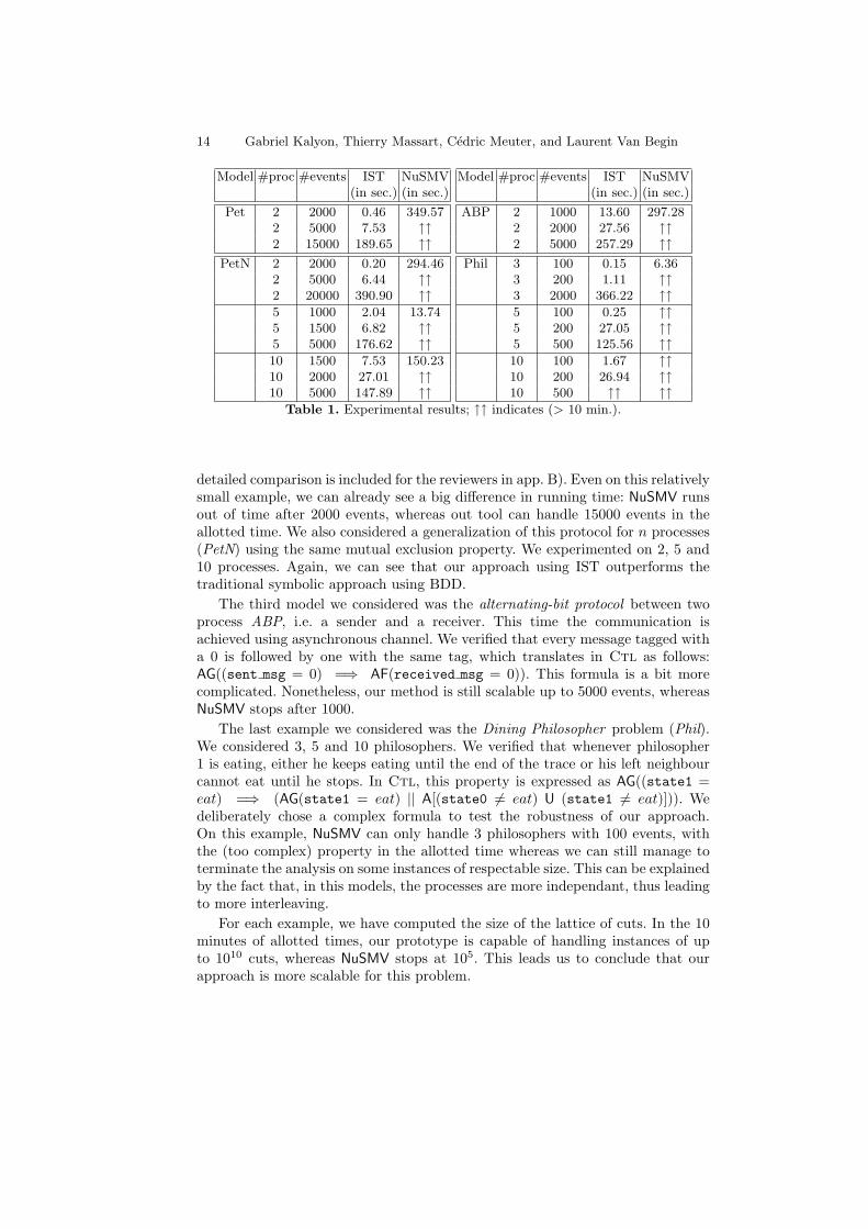
14 Gabriel Kalyon, Thierry Massart, Cedric Meuter, and Laurent Van Begin
Model #proc #events IST NuSMV(in sec.) (in sec.)
Pet 2 2000 0.46 349.572 5000 7.53 ↑↑2 15000 189.65 ↑↑
PetN 2 2000 0.20 294.462 5000 6.44 ↑↑2 20000 390.90 ↑↑5 1000 2.04 13.745 1500 6.82 ↑↑5 5000 176.62 ↑↑10 1500 7.53 150.2310 2000 27.01 ↑↑10 5000 147.89 ↑↑
Model #proc #events IST NuSMV(in sec.) (in sec.)
ABP 2 1000 13.60 297.282 2000 27.56 ↑↑2 5000 257.29 ↑↑
Phil 3 100 0.15 6.363 200 1.11 ↑↑3 2000 366.22 ↑↑5 100 0.25 ↑↑5 200 27.05 ↑↑5 500 125.56 ↑↑10 100 1.67 ↑↑10 200 26.94 ↑↑10 500 ↑↑ ↑↑
Table 1. Experimental results; ↑↑ indicates (> 10 min.).
detailed comparison is included for the reviewers in app. B). Even on this relativelysmall example, we can already see a big difference in running time: NuSMV runsout of time after 2000 events, whereas out tool can handle 15000 events in theallotted time. We also considered a generalization of this protocol for n processes(PetN) using the same mutual exclusion property. We experimented on 2, 5 and10 processes. Again, we can see that our approach using IST outperforms thetraditional symbolic approach using BDD.
The third model we considered was the alternating-bit protocol between twoprocess ABP, i.e. a sender and a receiver. This time the communication isachieved using asynchronous channel. We verified that every message tagged witha 0 is followed by one with the same tag, which translates in Ctl as follows:AG((sent msg = 0) =⇒ AF(received msg = 0)). This formula is a bit morecomplicated. Nonetheless, our method is still scalable up to 5000 events, whereasNuSMV stops after 1000.
The last example we considered was the Dining Philosopher problem (Phil).We considered 3, 5 and 10 philosophers. We verified that whenever philosopher1 is eating, either he keeps eating until the end of the trace or his left neighbourcannot eat until he stops. In Ctl, this property is expressed as AG((state1 =eat) =⇒ (AG(state1 = eat) || A[(state0 6= eat) U (state1 6= eat)])). Wedeliberately chose a complex formula to test the robustness of our approach.On this example, NuSMV can only handle 3 philosophers with 100 events, withthe (too complex) property in the allotted time whereas we can still manage toterminate the analysis on some instances of respectable size. This can be explainedby the fact that, in this models, the processes are more independant, thus leadingto more interleaving.
For each example, we have computed the size of the lattice of cuts. In the 10minutes of allotted times, our prototype is capable of handling instances of upto 1010 cuts, whereas NuSMV stops at 105. This leads us to conclude that ourapproach is more scalable for this problem.

Testing Distributed Systems through Symbolic Model Checking of Traces 15
7 Future works
As future works, our symbolic method using IST will be intergrated in our toolTraX 1 and will be fully interfaced with our distributed controllers design environ-ment dSL [1, 2] to allow efficient testing of real industrial distributed controllers.We will also continue to investiguate possible further improvements of our tech-nique, as the one inspired on the RCtl model checking with computation slicingdescribed in [14]. We also intend to investigate the use of our method in differ-ent frameworks. A first candidate is the validation of Message Sequence Charts(MSC). We must study how our method can improve the efficiency of existingMSC validation methods.
Finally, from a theoretical point of view, the exact complexity class of Ctlover partial order trace is not known. We plan to determine that full Ctl andsome interesting fragments (like RCtl).
References
1. De Wachter, B., Massart, T., Meuter, C.: dsl : An environment with automatic codedistribution for industrial control systems. In: Lecture Notes in Computer Sciences.Volume 3144. Springer (2004) 132–145 (14 pages).
2. De Wachter, B., Genon, A., Massart, T., Meuter, C.: The formal design of distributedcontrollers with dsl and spin. Formal Aspects of Computing 17(2) (2005) 177–200(24 pages).
3. Holzmann, G.J.: The model checker spin. IEEE Trans. Software Eng. 23(5) (1997)279–295
4. McMillan, K.: The smv system. Technical Report CMU-CS-92-131, Carnegie MellonUniversity (1992)
5. Cimatti, A., Clarke, E.M., Giunchiglia, E., Giunchiglia, F., Pistore, M., Roveri, M.,Sebastiani, R., Tacchella, A.: Nusmv 2: An opensource tool for symbolic modelchecking. In: CAV. (2002) 359–364
6. Godefroid, P.: Partial-Order Methods for the Verification of Concurrent Systems- An Approach to the State-Explosion Problem. Volume 1032 of Lecture Notes inComputer Science. Springer (1996)
7. Valmari, A.: On-the-fly verification with stubborn sets. In: CAV. (1993) 397–408
8. Clarke, E., Grumberg, O., Peled, D.: Model Checking. The MIT Press (1999)
9. McMillan, K.L.: Symbolic model checking: an approach to the state explosion prob-lem. Carnegie Mellon University (1992)
10. Bryant, R.E.: Symbolic boolean manipulation with ordered binary-decision dia-grams. ACM Comput. Surv. 24(3) (1992) 293–318
11. Lamport, L.: Time, clocks, and the ordering of events in a distributed system.Commun. ACM 21(7) (1978) 558–565
12. Mattern, F.: Virtual time and global states of distributed systems. In et al., C.M.,ed.: Proc. Workshop on Parallel and Distributed Algorithms, North-Holland / El-sevier (1989) 215–226
13. Chase, C.M., Garg, V.K.: Detection of global predicates: Techniques and theirlimitations. Distributed Computing 11(4) (1998) 191–201
1 http://www.ulb.ac.be/di/ssd/cmeuter/trax/

16 Gabriel Kalyon, Thierry Massart, Cedric Meuter, and Laurent Van Begin
14. Sen, A., Garg, V.K.: Detecting temporal logic predicates in distributed programsusing computation slicing. In: OPODIS. (2003) 171–183
15. Clarke, E.M., Emerson, E.A.: Design and synthesis of synchronization skeletonsusing branching-time temporal logic. In: Logic of Programs. (1981) 52–71
16. Mittal, N., Garg, V.K.: Computation slicing: Techniques and theory. In: DISC.(2001) 78–92
17. Ganty, P., Meuter, C., Begin, L.V., Kalyon, G., Raskin, J.F., Delzanno, G.: Symbolicdata structure for sets of k-uples of integers. Technical report, Universite Libre deBruxelles (2006)
18. Ganty, P.: Algorithmes et structures de donnees efficaces pour la manipulation decontraintes sur les intervalles. Master’s thesis, Universite Libre de Bruxelles (2002)
19. Mazurkiewicz, A.W.: Trace theory. In: Advances in Petri Nets. (1986) 279–32420. Thiagarajan, P.S.: A trace based extension of linear time temporal logic. In Abram-
sky, S., ed.: Proceedings of the Ninth Annual IEEE Symp. on Logic in ComputerScience, LICS 1994, IEEE Computer Society Press (1994) 438–447
21. Alur, R., Peled, D., Penczek, W.: Model checking of causality properties. In:Proceedings of the 10th Annual IEEE Symposium on Logic in Computer Science(LICS’95), San Diego, California (1995) 90–100
22. Niebert, P., Peled, D.: Efficient model checking for ltl with partial order snapshots.In Hermanns, H., Palsberg, J., eds.: TACAS. Volume 3920 of Lecture Notes inComputer Science., Springer (2006) 272–286
23. Thiagarajan, P.S., Walukiewicz, I.: An expressively complete linear time temporallogic for mazurkiewicz traces. Inf. Comput. 179(2) (2002) 230–249
24. Diekert, V., Gastin, P.: LTL is expressively complete for Mazurkiewicz traces. Jour-nal of Computer and System Sciences 64(2) (2002) 396–418
25. Chandy, K.M., Lamport, L.: Distributed snapshots: Determining global states ofdistributed systems. ACM Trans. Comput. Syst. 3(1) (1985) 63–75
26. Charron-Bost, B., Delporte-Gallet, C., Fauconnier, H.: Local and temporal predi-cates in distributed systems. ACM Trans. Program. Lang. Syst. 17(1) (1995)
27. Garg, V.K., Waldecker, B.: Detection of weak unstable predicates in distributedprograms. IEEE Trans. Parallel Distrib. Syst. 5(3) (1994) 299–307
28. Garg, V.K., Waldecker, B.: Detection of strong unstable predicates in distributedprograms. IEEE Trans. Parallel Distrib. Syst. 7(12) (1996) 1323–1333
29. Garg, V.K., Mittal, N.: On slicing a distributed computation. In: ICDCS. (2001)322–329
30. Jard, C., Jeron, T., Jourdan, G.V., Rampon, J.X.: A general approach to trace-checking in distributed computing systems. In: ICDCS. (1994) 396–403
31. Sen, K., Rosu, G., Agha, G.: Online efficient predictive safety analysis of multi-threaded programs. In: TACAS. (2004) 123–138
32. Sen, K., Rosu, G., Agha, G.: Detecting errors in multithreaded programs by gener-alized predictive analysis of executions. In: FMOODS. (2005) 211–226
33. Genon, A., Massart, T., Meuter, C.: Monitoring distributed controllers: When anefficient ltl algorithm on sequences is needed to model-check traces. In Misra, J.,Nipkow, T., Sekerinski, E., eds.: FM. Volume 4085 of Lecture Notes in ComputerScience., Springer (2006) 557–572
34. Zampunieris, D., Le Charlier, B.: Efficient handling of large sets of tuples withsharing trees. In: Proceedings of the 5th Data Compression Conference (DCC’95),IEEE Computer Society Press (1995) 428
35. Ammirati, P., Delzanno, G., Ganty, P., Geeraerts, G., Raskin, J.F., Van Begin, L.:Babylon: An integrated toolkit for the specification and verification of parameterizedsystems. In: 2nd workshop on Specification, Analysis and Validation for Emergingtechnologies (SAVE02). (2002)
Testing Distributed Systems through Symbolic Model Checking of Traces 17
A Proofs of section 5
A.1 Preliminary results
Before presenting the proofs of sec. 5, we need to establish a few preliminaries.First, for a k-uple −→x , we note C−→x = {e ∈ E | pos(e) ≤ xpid(e)} the subset ofevents represented by −→x represents. We will also need the following results.
Lemma 11. Given a trace T = 〈E,α,�〉, and a process Pi ⊆ E, we have that∀C ∈ cuts(T) : enabled(C)∩Pi ⊆ {e} where e ∈ E is such that pos(e) = |C∩Pi|+1.
Proof. First, note that enabled(C) ∩ Pi ⊆ Pi. We therefore only consider eventsof Pi. Let e be such an event. If pos(e) < |C ∩ Pi| + 1, we have that that e ∈ Cwhich implies e 6∈ enabled(C). On the other hand pos(e) > |C ∩ Pi|+ 1, the evente′. such that pos(e′) = |C ∩ Pi| + 1 does not belong to C but is in ↓e \ {e} andagain e 6∈ enabled(C). The only remaining possibility is that pos(e) = |C ∩Pi|+1.
Lemma 12. Given a trace T = 〈E,α,�〉 of k processes and C,C ′ ∈ cuts(T),if C ⊆ C ′ then there exists a sequence C0, C1, C2, . . . , Cm such that (C = C0) ∧(Cm = C ′) ∧ (∀i ∈ [1,m] : (Ci−1 ∈ pre∃({Ci})) ∧ (Ci ∈ cuts(T))).
Proof. We proceed by induction on |C ′ \ C|
– base case: if |C ′ \ C| = 0, then C = C ′ and the proof is immediate. Thesequence is simply C = C0 = Cm = C ′.
– induction step: if |C ′ \C| = n, we have that ∃e ∈ (C ′ \C) : e ∈ enabled(C).Indeed, since � is a partial order, and since |C ′ \ C| is non-empty, we knowthat (C ′ \ C) has at least one minimal element, i.e. an event e such that@e′ ∈ (C ′ \ C) : e′ ≺ e. Since C ′ is a cut and e ∈ C ′, we have that ↓e ∈ C ′
and since e is minimal in C ′ \ C, that ↓e \ {e} ∈ C. It follows directly thate ∈ enabled(C). We know therefore that C ∪ {e} ∈ cuts(T) and since e ∈C ′ \ C that C ∪ {e} ⊆ C ′. By induction there exists a sequence C0, ..., Cn−1
of cuts between C ∪ {e} and C ′. The sequence for C, C ′ is then given byC,C0, ..., Cn−1.
A.2 Proof of lemma 1
Given a trace T = 〈E,α,�〉, we have that:
sets(I>) = [[>]]
Proof. First, note that [[>]] = {C ∈ cuts(T) | C |= >} = cuts(T). Therefore, prov-ing sets(I>) = [[>]] amounts to proving that sets(I>) = cuts(T). Consequently,we prove the inclusion in both ways:
– For cuts(T) ⊆ sets(I>), we prove that cuts(T) ⊆ sets(I) is an invariant of thealgorithm. At the initial step, we start with I = I0. It can be easily proventhat sets(I0) = {C ⊆ E | ∀e ∈ C :↓e∩Ppid(e) ⊆ C}. Condition (i) of definition1 then implies that every �-closed subset of E belongs to sets(I0). Therefore,
18 Gabriel Kalyon, Thierry Massart, Cedric Meuter, and Laurent Van Begin
we have that cuts(T) ⊆ sets(I0). Then, at each step of the algorithm, weremove cuts from I to take into account a communication e →c e′. For thatwe compute two ISTs B(e) and A(e′). It can be easily proven that sets(B(e)) ={C ∈ sets(I0) | e 6∈ C} and that sets(A(e′)) = {C ∈ sets(I0) | e′ ∈ C}. Thus,sets(A(e′) ∩ B(e)) = sets(A(e′)) ∩ sets(B(e)) = {C ∈ sets(I0) | (e′ ∈ C) ∧ (e 6∈C)}. Therefore, since e � e′, any C ∈ sets(A(e′) ∩ B(e)) is not �-closed. Itfollows directly that sets(A(e′) ∩ B(e)) ∩ cuts(T) = ∅, and that cuts(T) ⊆sets(I \ (A(e′) ∩ B(e))). We can therefore conclude that cuts(T) ⊆ sets(I) isan invariant and finally that cuts(T) ⊆ sets(I>).
– For sets(I>) ⊆ cuts(T), we equivalently prove that ∀C ⊆ E : (C 6∈ cuts(T)) ⇒(C 6∈ sets(I>)). If C 6∈ cuts(T), then ∃e ∈ C, e′ ∈↓e : e′ 6∈ C. In this case,since e′ ∈↓e, there exists in T a sequence of event e′ = e1, e2, ..., e` = e and∀i ∈ [1, `) : ei → ei+1. Moreover, since e′ 6∈ C, ∃i ∈ [1, `) : (ei+1 ∈ C) ∧ (ei 6∈C). From there, we have two cases:(i) if pid(ei) = pid(ei+1), then C cannot be represented using a k-uple. In-
deed, let (x1, x2, ..., xk) be such an hypothetical k-uple. If ei+1 ∈ C, thenpos(ei+1) ≤ xpid(ei+1). But since ei → ei+1, pos(ei) ≤ pos(ei+1) and ei isalso in C. In this case, we therefore know that C 6∈ sets(I>).
(ii) on the other hand, if pid(ei) 6= pid(ei+1), then there is a communicationei →c ei+1. Thus, in some step of the algorithm, we will compute B(ei)and A(ei+1) such that sets(A(ei+1) ∩ B(ei)) = {C ∈ sets(I0) | (ei+1 ∈C) ∧ (ei 6∈ C)}. Therefore, C will be removed at this step.
In both case, C 6∈ sets(I>) and we can conclude that sets(I>) ⊆ cuts(T)
A.3 Proof of lemma 2
Given a trace T = 〈E,α,�〉 and a predicate p, we have that
sets(Ip) = [[p]]
Proof. We need to prove the inclusion in both ways:
– For sets(Ip) ⊆ [[p]], we prove equivalently that ∀C ∈ sets(Ip) : C |= p. Firstnote that ∀C ∈ sets(Ip) : C ∈ sets(I>) = cuts(T). Therefore, C is �-closed.Then, we have three possibilities:(i) C ∈ sets(B(es1)): in this case, since es1 = e1 6∈ C and since C is �-
closed, we have that vC(p) = v∅(p). However, since C was added to Ip,by construction we have that ∅ |= p which in turn implies that C |= p.
(ii) ∃i ∈ [1, `) : C ∈ sets(A(esi) ∩ B(esi+1)): in this case, since esi
∈ C,esi+1 6∈ C and since C is �-closed, we have that {ej | j ∈ [si, si+1)} ⊆ C.However, by construction, ∀j ∈ [si, si+1) :↓ej |= p. Thus, if Ci denotes↓esi , it follows that vC(p) = vCi(p), which in turn implies C |= p.
(iii) C ∈ sets(A(es`)) : in this case since es`
= em ∈ C and since C �-closed, vC(p) = vE(p). However, since C was added to Ip, we know byconstruction that E |= p, which in turn implies that C |= p.
– For [[p]] ⊆ sets(Ip), we prove equivalently that ∀C ∈ cuts(T) : (C |= p) ⇒(C ∈ sets(Ip)). Again, we have three possibilities:

Testing Distributed Systems through Symbolic Model Checking of Traces 19
(i) C ∩ Ep = ∅ : in this case, we have that vC(p) = v∅(p) and C |= p, that∅ |= p. Therefore, since C ∈ B(es1) and since C ∈ cuts(T) = sets(I>), wecan conclude that C ∈ sets(Ip).
(ii) ∅ 6= C ∩ Ep 6= Ep : in this case, let i = max≤({j ∈ [1, `) | esj ∈ C}).Since esj ∈ C, we have that C ∈ sets(A(esj )). Moreover, we knowthat esi+1 6∈ C, otherwise, i would not be maximal. It follows thatC ∈ sets(B(esi+1)) and that C ∈ sets(A(esi) ∩ B(esi+1)). However, if Ci
denotes ↓esi , since C |= p and vC(p) = vCi(p), we have that Ci |= p.Therefore, A(esi) ∩ B(esi+1) will be added to Ip in the construction. Fi-nally, since C ∈ cuts(T) = sets(I>), we can conclude that C ∈ sets(Ip).
(iii) C ∩ Ep = Ep : in this case, we have that vC(p) = vE(p) and since C |=p, that E |= p. Therefore, since C ∈ A(es`
) and since C ∈ cuts(T) =sets(I>), we can conclude that C ∈ sets(Ip).
A.4 Proof of lemma 3
Given a trace T = 〈E,α,�〉 and Ctl formulae φ, φ1 and φ2, we have that:
sets(Iφ1∨φ2) = [[φ1 ∪ φ2]]sets(Iφ1∧φ2) = [[φ1 ∩ φ2]]
sets(I¬φ) = [[¬φ]]
Proof. This is a direct consequence of the following equalities:
sets(I¬φ) = sets(Iφ ∩ I>)= sets(Iφ) ∩ sets(I>)= (sets(Nk) \ sets(Iφ)) ∩ sets(I>)= (sets(Nk) ∩ sets(I>)) \ (sets(Iφ) ∩ sets(I>))= sets(I>) \ sets(Iφ)= [[>]] \ [[φ]]= [[¬φ]]
sets(Iφ1∨φ2) = sets(Iφ1 ∪ Iφ2)= sets(Iφ1) ∪ sets(Iφ2)= [[φ1]] ∪ [[φ2]]= [[φ1 ∨ φ2]]
sets(Iφ1∧φ2) = sets(Iφ1 ∩ Iφ2)= sets(Iφ1) ∩ sets(Iφ2)= [[φ1]] ∩ [[φ2]]= [[φ1 ∧ φ2]]
A.5 Proof of lemma 4
Given a trace T = 〈E,α,�〉 and a subset X ⊆ cuts(T), we have that:
pre∃(X) =⋃
i∈[1,k]
pre∃i (X)

20 Gabriel Kalyon, Thierry Massart, Cedric Meuter, and Laurent Van Begin
Proof. This is direct consequence of the following equalities:
pre∃(X) = {C ∈ cuts(T) | ∃e ∈ enabled(C) : C ∪ {e} ∈ X}= {C ∈ cuts(T) | ∃e ∈ enabled(C) ∩ E : C ∪ {e} ∈ X}= {C ∈ cuts(T) | ∃e ∈ enabled(C) ∩ (
⋃i∈[1,k] Pi) : C ∪ {e} ∈ X}
= {C ∈ cuts(T) | ∃e ∈⋃
i∈[1,k](enabled(C) ∩ (Pi) : C ∪ {e} ∈ X}=
⋃i∈[1,k]{C ∈ cuts(T) | ∃e ∈ enabled(C) ∩ Pi : C ∪ {e} ∈ X}
=⋃
i∈[1,k] pre∃i (X)
A.6 Proof of lemma 5
Given a trace T = 〈E,α,�〉, and an IST I such that setsI ⊆ cuts(T), we havethat:
pre∃i (sets(I)) = sets(I [xi←xi−1] ∩ I>)
Proof. This is a direct consequence of the following equivalences:
sets(I [xi←xi−1] ∩ I>)= {C ∈ cuts(T) | ∃−→x ∈ tuple(I [xi←xi−1]) : C = C−→x }= {C ∈ cuts(T) | ∃−→x ′ ∈ tuple(I) : C = C−→x ′ \ {e ∈ Pi | pos(e) = x′i}}= {C ∈ cuts(T) | ∃−→x ′ ∈ tuple(I) : C = C−→x ′ \ {e ∈ Pi | pos(e) = |C−→x ′ ∩ Pi|}}= {C ∈ cuts(T) | ∃−→x ′ ∈ tuple(I) : C = C−→x ′ \ {e ∈ Pi | pos(e) = |C ∩ Pi|+ 1}}= {C ∈ cuts(T) | ∃−→x ′ ∈ tuple(I) : C−→x ′ = C ∪ {e ∈ Pi | pos(e) = |C ∩ Pi|+ 1}}= {C ∈ cuts(T) | ∃C ′ ∈ sets(I) : C ′ = C ∪ {e ∈ Pi | pos(e) = |C ∩ Pi|+ 1}}
(by lem. 11)= {C ∈ cuts(T) | ∃e ∈ enabled(C) ∩ Pi,∃C ′ ∈ sets(I) : C ′ = C ∪ {e}}= {C ∈ cuts(T) | ∃e ∈ enabled(C) ∩ Pi : C ∪ {e} ∈ sets(I)}= pre∃i (sets(I))
A.7 Proof of lemma 6
Given a trace T = 〈E,α,�〉, and an subset X ⊆ cuts(T), we have that
pre∀(X) =⋂
i∈[1,k]
pre∀i (X)

Testing Distributed Systems through Symbolic Model Checking of Traces 21
Proof. This is a direct consequence of the following equalities:
pre∀(X) = {C ∈ cuts(T) | ∀e ∈ enabled(C) : C ∪ {e} ∈ X}= {C ∈ cuts(T) | ¬(∃e ∈ enabled(C) : C ∪ {e} 6∈ X)}= {C ∈ cuts(T) | ¬(∃e ∈ enabled(C) : C ∪ {e} ∈ (cuts(T) \X))}= {C ∈ cuts(T) | ¬(C ∈ pre∃(cuts(T) \X))}= cuts(T) \ pre∃(cuts(T) \X)= cuts(T) \
(⋃i∈[1,k] pre
∃i (cuts(T) \X)
)=
⋂i∈[1,k]
(cuts(T) \ pre∃i (cuts(T) \X)
)=
⋂i∈[1,k] (cuts(T) \ {C ∈ cuts(T) | ∃e ∈ enabled(C) ∩ Pi : C ∪ {e} ∈ cuts(T) \X})
=⋂
i∈[1,k] (cuts(T) \ {C ∈ cuts(T) | ∃e ∈ enabled(C) ∩ Pi : C ∪ {e} 6∈ X})=
⋂i∈[1,k] (cuts(T) \ {C ∈ cuts(T) | ¬(∀e ∈ enabled(C) ∩ Pi : C ∪ {e} ∈ X}))
=⋂
i∈[1,k]
(cuts(T) \ {C ∈ cuts(T) | ¬(C ∈ pre∀i (X)}
)=
⋂i∈[1,k]
(cuts(T) \ (cuts(T) \ pre∀i (X))
)=
⋂i∈[1,k] pre
∀i (X)
A.8 Proof of lemma 7
Given a trace T = 〈E,α,�〉, and an subset X ⊆ cuts(T), we have that
pre∀i (X) = pre∃i (X) ∪ blockedi
Proof. We proceed by proving inclusion in both ways.
– For pre∀i (X) ⊆ pre∃i (X) ∪ blockedi, let us examine a cut C ∈ pre∀i (X). Either,enabled(C) ∩ Pi = ∅, in which case, C ∈ blockedi, or enabled(C) ∩ Pi 6= ∅, inwhich case ∃e ∈ enabled(C) ∩ Pi : C ∪ {e} ∈ X holds, which, in turn, impliesthat C ∈ pre∃i (X).
– For pre∃i (X)∪blockedi ⊆ pre∀i (X), we prove that blockedi ⊆ pre∀i (X) and thatpre∃i (X) ⊆ pre∀i (X) independently. The proof for blockedi is straightforward.Indeed, for a cut C ∈ blockedi, we know that enabled(C) ∩ Pi = ∅. Theuniversal quantification over enabled(C) ∩ Pi in pre∀i (X) is therefore triviallysatisfied, and C ∈ pre∀i (X). The proof for prei(X) is also quite simple. For acut C ∈ pre∃i (X), we know that ∃e ∈ enabled(C) ∩ Pi : C ∪ {e} ∈ X. Thisimplies that e ∈ enabled(C)∩Pi 6= ∅. The only possibility for enabled(C)∩Pi isa singleton containing the next event of Pi, by lem.11. Therefore we have that∃e ∈ enabled(C)∩Pi : C∪{e} ∈ X implies ∀e ∈ enabled(C)∩Pi : C∪{e} ∈ X,which, in turn implies C ∈ pre∀i (X).
A.9 Proof of lemma 8
Given a trace T = 〈E,α,�〉 and a process Pi ⊆ E, we have that C ∈ blockedi ifand only if:
∀e ∈ E ∩ Pi : (pos(e) = |C ∩ Pi|+ 1) =⇒ (∃e′ ∈ E \ C : e′ →c e)
Proof. We prove the equivalence in both ways.

22 Gabriel Kalyon, Thierry Massart, Cedric Meuter, and Laurent Van Begin
– (⇐) Let us examine a cut C such that ∀e ∈ E∩Pi : (pos(e) = |C∩Pi|+1) =⇒(∃e′ ∈ E \C : e′ →c e). By lem. 11, we know that enabled(C)∩Pi ⊆ {e} wheree is such that pos(e) = |C ∩ Pi|+ 1. We have then that ∃e′ ∈ E \C : e′ →c e.Since e′ 6∈ C and since e′ →c e implies that e′ � e, we have that e 6∈ enabled(C)hence enabled(C) ∩ Pi = ∅ and C ∈ blockedi.
– (⇒) We proceed by proving the contraposition. Let us examine a cut C suchthat ∃e ∈ E ∩ Pi : (pos(e) = |C ∩ Pi| + 1) ∧ (∀e′ ∈ E \ C : e′ 6→c e). Sincepos(e) > |C ∩ Pi|, we can conclude that e 6∈ C. Moreover, since C ∈ cuts(T),we have that ∀e′ ∈ Pi : (pos(e′) ≤ |C∩Pi|) =⇒ (e′ ∈ C). Finally, ∀e′ ∈ E\C :e′ 6→c e implies that @e′ ∈ E \Pi : e′ � e. We can deduce that e ∈ enabled(C)and that enabled(C) ∩ Pi 6= ∅, which implies that C 6∈ blockedi.
A.10 Proof of lemma 9
Given a trace T = 〈E,α,�〉, and an IST I such that I ⊆ cuts(T), we have that:
pre∀i (sets(I)) = sets((I [xi←xi−1] ∩ I>) ∪ Iblockedi)
Proof. This is a direct consequence of the following equalities:
pre∀(sets(I)) = pre∃i (sets(I)) ∪ blockedi (by lem. 7)= sets(I [xi←xi−1] ∩ I>) ∪ blockedi (by lem. 5)= sets(I [xi←xi−1] ∩ I>) ∪ sets(Iblockedi) (by constr. of Iblockedi)= sets((I [xi←xi−1] ∩ I>) ∪ Iblockedi
)
A.11 Proof of lemma 10
Given a trace T = 〈E,α,�〉 of k processes and a Ctl formula φ, we have that:
sets(IEFφ) = [[EFφ]]
Proof. This is a direct consequence of the following equalities:
sets(↓Iφ ∩ I>)= sets(↓Iφ) ∩ sets(I>)= sets({−→x ∈ Nk | ∃−→x ′ ∈ tuple(Iφ) : −→x ≤ −→x ′}) ∩ sets(I>)= {C ⊆ E | ∃C ′ ∈ sets(Iφ) : C ⊆ C ′} ∩ cuts(T)= {C ∈ cuts(T) | ∃C ′ ∈ sets(Iφ) : C ⊆ C ′}= {C ∈ cuts(T) | ∃C ′ ∈ [[φ]] : C ⊆ C ′}
(by lem. 12)
={
C ∈ cuts(T)∣∣∣∣ ∃C ′ ∈ [[φ]],∃C0, ..., Cm : (C0 = C) ∧ (Cm = C ′)∧(∀i ∈ [1,m] : (Ci−1 ∈ pre∃({Ci})) ∧ (Ci ∈ cuts(T)))
}= [[EFφ]]
Testing Distributed Systems through Symbolic Model Checking of Traces 23
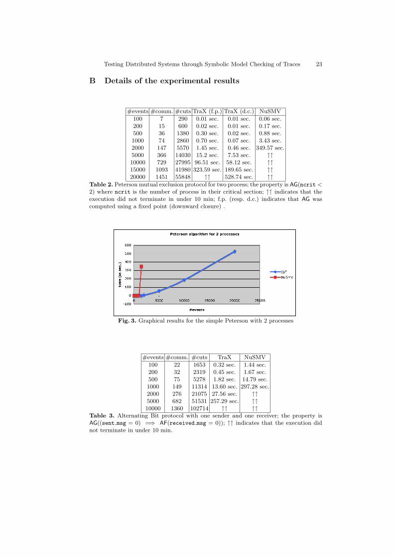
B Details of the experimental results
#events #comm. #cuts TraX (f.p.) TraX (d.c.) NuSMV
100 7 290 0.01 sec. 0.01 sec. 0.06 sec.200 15 600 0.02 sec. 0.01 sec. 0.17 sec.500 36 1380 0.30 sec. 0.02 sec. 0.88 sec.1000 74 2860 0.70 sec. 0.07 sec. 3.43 sec.2000 147 5570 1.45 sec. 0.46 sec. 349.57 sec.5000 366 14030 15.2 sec. 7.53 sec. ↑↑10000 729 27995 96.51 sec. 58.12 sec. ↑↑15000 1093 41980 323.59 sec. 189.65 sec. ↑↑20000 1451 55848 ↑↑ 528.74 sec. ↑↑
Table 2. Peterson mutual exclusion protocol for two process; the property is AG(ncrit <2) where ncrit is the number of process in their critical section; ↑↑ indicates that theexecution did not terminate in under 10 min; f.p. (resp. d.c.) indicates that AG wascomputed using a fixed point (downward closure) .
Fig. 3. Graphical results for the simple Peterson with 2 processes
#events #comm. #cuts TraX NuSMV
100 22 1653 0.32 sec. 1.44 sec.200 32 2319 0.45 sec. 1.67 sec.500 75 5278 1.82 sec. 14.79 sec.1000 149 11314 13.60 sec. 297.28 sec.2000 276 21075 27.56 sec. ↑↑5000 682 51531 257.29 sec. ↑↑10000 1360 102714 ↑↑ ↑↑
Table 3. Alternating Bit protocol with one sender and one receiver; the property isAG((sent msg = 0) =⇒ AF(received msg = 0)); ↑↑ indicates that the execution didnot terminate in under 10 min.

24 Gabriel Kalyon, Thierry Massart, Cedric Meuter, and Laurent Van Begin
#processes #events #comm #cuts TraX NuSMV
2 100 7 107 0.00 sec. 0.03 sec.2 200 14 206 0.00 sec. 0.09 sec.2 500 34 506 0.01 sec. 0.42 sec.2 1000 68 1016 0.04 sec. 2.80 sec.2 2000 134 2039 0.20 sec. 294.46 sec.2 5000 334 5106 6.44 sec. ↑↑2 10000 667 10047 48.10 sec. ↑↑2 20000 1335 20267 390.90 sec. ↑↑5 100 56 404 0.03 sec. 0.09 sec.5 200 97 1009 0.07 sec. 0.16 sec.5 500 202 2618 0.33 sec. 0.85 sec.5 1000 402 5393 2.04 sec. 13.74 sec.5 1500 602 11732 6.82 sec. ↑↑5 2000 773 13885 12.61 sec. ↑↑5 5000 1926 27835 176.62 sec. ↑↑5 10000 3801 55535 ↑↑ ↑↑10 100 328 14072 0.82 sec. 0.01 sec.10 200 314 22173 0.79 sec. 0.46 sec.10 500 493 43908 2.12 sec. 1.60 sec.10 1000 796 72567 5.42 sec. 4.20 sec.10 1500 1024 92340 7.53 sec. 150.23 sec.10 2000 1405 147219 27.01 sec. ↑↑10 5000 3255 203002 147.89 sec. ↑↑10 10000 6361 452897 ↑↑ ↑↑
Table 4. Peterson mutual exclusion protocol generalized for n process; the property isAG(ncrit < 2) where ncrit is the number of process in their critical section; ↑↑ indicatesthat the execution did not terminate in under 10 min.
Fig. 4. Graphical results for Peterson with 10 processes

Testing Distributed Systems through Symbolic Model Checking of Traces 25
#processes #events #comm #cuts TraX NuSMV
3 100 31 2060 0.15 6.363 200 61 5879 1.11 ↑↑3 500 160 11587 6.24 ↑↑3 1000 324 20780 28.90 ↑↑3 2000 613 55680 366.22 ↑↑3 5000 1654 104591 ↑↑ ↑↑5 100 65 41334 0.25 ↑↑5 200 101 405858 27.05 ↑↑5 500 229 1021052 125.56 ↑↑5 1000 547 1342108 ↑↑ ↑↑10 100 130 377853293 1.67 ↑↑10 200 189 797010724 26.94 ↑↑10 500 474 1478286661 ↑↑ ↑↑
Table 5. Dining philosophers using shared variables for the forks; the property isAG((state1 = eat) =⇒ (AG(state1 = eat) || A[(state0 6= eat) U (state1 6= eat)]))where statei is the state of philosopher i (eat, hungry or idle); ↑↑ indicates that theexecution did not terminate in under 10 min.


