Model Checking with Strong Fairness

Formal Methods in System Design, 28, 57–84, 2006c© 2006 Springer Science + Business Media, Inc. Manufactured in The Netherlands.

Model Checking with Strong Fairness∗

YONIT KESTEN† [email protected] Gurion University

AMIR PNUELI [email protected] RAVIVELAD SHAHAR [email protected] Institute of Science

Abstract. In this paper we present a coherent framework for symbolic model checking of linear-time tempo-ral logic (LTL) properties over finite state reactive systems, taking full fairness constraints into consideration.We use the computational model of a fair discrete system (FDS) which takes into account both justice (weakfairness) and compassion (strong fairness). The approach presented here reduces the model-checking probleminto the question of whether a given FDS is feasible (i.e. has at least one computation).

The contribution of the paper is twofold: On the methodological level, it presents a direct self-containedexposition of full LTL symbolic model checking without resorting to reductions to either μ-calculus or CTL.On the technical level, it extends previous methods by dealing with compassion at the algorithmic level insteadof either adding it to the specification, or transforming compassion to justice.

Finally, we extend CTL∗ with past operators, and show that the basic symbolic feasibility algorithm presentedhere, can be used to model check an arbitrary CTL∗ formula over an FDS with full fairness constraints.

Keywords: model checking, temporal logic, LTL, CTL, fairness, fair discrete systems, temporal testers

1. Introduction

Two kinds of temporal logics have been proposed over the years for specifying theproperties of reactive systems: the linear time logic LTL [8] and the branching timevariant CTL [2]. Also two methods for the formal verification of the temporal propertiesof reactive systems have been developed: the deductive approach based on interactivetheorem proving, and the fully automatic algorithmic approach, widely known as modelchecking. Tracing the evolution of these ideas, we find that the deductive approachadopted LTL as its main vehicle for specification, while the model-checking approachused CTL as the specification language [2, 23].

This is more than a historical coincidence or a matter of personal preference. The mainadvantage of CTL for model checking is that it is state-based and, therefore, the processof verification can be performed by straightforward labeling of the existing states inthe discrete structure, leading to no further expansion or unwinding of the structure. Incontrast, LTL is path-based and, since many paths can pass through a single state, labelinga structure by the LTL sub-formulas it satisfies necessarily requires splitting the state into

∗This research was supported in part by an infra-structure grant from the Israeli Ministry of Science and Art,a grant from the U.S.-Israel Binational Science Foundation, and a gift from Intel.†Author to whom all correspondence should be addressed.

58 KESTEN ET AL.

several copies. This is the reason why the development of model-checking algorithmsfor LTL always lagged several years behind their first introduction for the CTL logic.

The first model-checking algorithms were based on the enumerative approach, con-structing an explicit representation of all reachable states of the considered system [2],and were developed for the branching-time temporal logic CTL. The LTL version of thesealgorithms was developed in [16] for the future fragment of propositional LTL (PTL),and extended in [18] to the full PTL. The basic fixed-point computation algorithm forthe identification of fair computations presented in [16], was developed independentlyin [6] for FCTL (fair CTL).

Observing that upgrading from justice to full fairness (i.e., adding compassion) isreflected in the automata view of verification as an upgrade from a Buchi to a Streettautomaton, we can view the algorithms presented in [6] and [16] as algorithms for check-ing the emptiness of Streett automata [26]. An improved algorithm solving the relatedproblem of emptiness of Streett automata, was later presented in [10]. The developmentof the impressively efficient symbolic verification methods and their application to CTL

[1] raised the question whether a similar approach can be applied to PTL. The first sat-isfactory answer to this question is given in [1], by showing a reduction of PTL (futurefragment) model checking into μ-calculus model checking. A similar transformationfrom LTL to CTL model checking, is presented in [3]. The advantage of this approach isthat, following a preliminary transformation of the PTL formula and the given system,the algorithm proceeds by using available and efficient CTL symbolic model checkerssuch as SMV.

A certain weakness of all the available symbolic model checkers is that, in their rep-resentation of fairness, they only consider the concept of justice (weak fairness). Assuggested by many researchers, another important fairness requirement is that of com-passion (strong fairness) (e.g., [7, 8, 17]). This type of fairness is particularly useful in theanalysis of systems that use semaphores, synchronous communication, and other specialcoordination primitives. A partial answer to this criticism is that, since compassion canbe expressed in LTL (but not in CTL), once we developed a model-checking method forLTL, we can always add the compassion requirements as an antecedent to the propertywe wish to verify. A similar answer is standardly given for symbolic model checkersthat use the μ-calculus as their specification language, because compassion can also beexpressed as a μ-calculus formula [25]. The only question remaining is how practicalthis is.

In this paper we present an approach to the symbolic model checking of LTL formu-las, which takes into account full fairness, including both justice and compassion. Theapproach is self-contained and does not depend on a reduction to either μ-calculus orCTL model checking (as in [1] and [3], respectively). The main advantage of such aself-contained approach is that the end users no longer need to deal with two differentkinds of logics.

The treatment of the LTL component is essentially that of a symbolic constructionof a tableau by assigning a new auxiliary variable to each temporal sub-formula of theproperty we wish to verify. In that, our approach resembles very much the reductionmethod used in [1, 3] which, in turn, is an extension of the statification method used in[19] and [21] to deal with the past fragment of LTL. The model-checking problem is thenreduced into the question of feasibility of an FDS. The symbolic feasibility algorithm,

MODEL CHECKING WITH STRONG FAIRNESS 59

similar to the enumerative algorithm of [16], identifies all computations satisfying agiven set of fairness constraints. This involves the identification of all fair stronglyconnected subgraphs (SCS). However, while the enumerative algorithm identifies eachSCS separately, the BDD-based symbolic algorithm is more efficient, identifying all statesparticipating in some fair SCS simultaneously. Our symbolic algorithm can be viewed asa straightforward implementation of the nested fixed-point characterization of Emerson-Lei for fully fair computations [5], as opposed to the CTL model checkers which consideronly the weak-fairness part of this characterization.

Other works related to the approach developed here are presented in [9, 11], whereBDD-based symbolic algorithms for bad cycle detection are presented. They are based onthe fixed-point characterization of Emerson-Lei. These algorithms solve the problem offinding all those cycles within the computation graph, which satisfy a given set of weakfairness constraints. [9] gives heuristics which improve the performance of the Emerson-Lei algorithm. We use the same heuristics in our algorithm, while dealing with bothtypes of fairness constraints. [9, 11] can deal with strong fairness by reduction to weakfairness. According to the automata-theoretic view, [9] presents a symbolic algorithmfor the problem of emptiness of Buchi automata, while the algorithms presented hereprovide a symbolic solution to the emptiness problem of Streett automata.

An algorithm for dealing with compassion at the algorithmic level is presented in [14],however it is enumerative whereas our work provides a symbolic solution.

In [6], Emerson and Lei observed that the problem of CTL∗ model checking of finitestate systems can be resolved by recursive calls to an LTL model-checking algorithm. Tak-ing a similar approach, we augment CTL∗ with past operators and show that the symbolicfeasibility algorithm presented here, can be used to model check an arbitrary CTL∗ for-mula over a finite state FDS D, taking the full fairness constraints ofD into consideration.

We present a symbolic algorithm for finding a counter example for an LTL formula.The counter example is a finite path from an initial state to a fair cycle. In [4] a similaralgorithm is presented in the context of CTL, evaluating either a witness to an existentialproperty or a counter example for a universal property. The main difference betweenour algorithm and [4] is that we search for a fair cycle embedded within a terminalstrongly connected component while [4] look for a cycle embedded within the entire setof feasible states. Their search may fail several times before a fair cycle is found. Oursearch is guaranteed to succeed on the first trial.

The rest of the paper is organized as follows. In Section 2 we present the computa-tional model of fair discrete systems (FDS). In Section 3 we present PTL, the propositionalfragment of linear temporal logic, including the past operators. Next, in Section 4 wediscuss the construction of a tester for a PTL formula ϕ, which is an FDS characterizingall the sequences which satisfy ϕ. Having transformed the model-checking probleminto the feasibility problem of an FDS, we present the symbolic feasibility algorithmin Section 5, followed by an algorithm for extracting a witness (a counter example)in Section 6. In Section 7 we augment CTL∗ with past operators and use the feasibilityalgorithm to model check an arbitrary CTL∗ formulas over a finite state FDS. We concludein Section 8 with some experimental results, comparing the different methods used todeal with compassion requirements.

A (partial) conference version of this paper appeared in [13].

60 KESTEN ET AL.

2. Fair discrete systems

As a computational model for reactive systems, we take the model of fair discrete system(FDS). The computational model is used for modeling both the verified system and thetemporal properties. The FDS model replaces the earlier model of fair transition system(FTS) presented in [20] and [21]. The main difference between these two models is inthe representation of fairness constraints. The advantage of the new representation is thatit enables a unified representation of fairness constraints arising from both the systembeing verified, and the temporal property.

An FDS D : 〈V, �, ρ,J , C〉 consists of the following components:

• V = {u1, . . . , un}: A finite set of typed state variables ranging over finite domains. Wedefine a state s to be a type-consistent interpretation of V , assigning to each variableu ∈ V a value s[u] in its domain. We denote by � the set of all states.

• �: The initial condition. This is an assertion characterizing all the initial states of D.A state is called initial if it satisfies �.

• ρ: A transition relation. This is an assertion ρ(V, V ′), relating a state s ∈ � to itsD-successor s ′ ∈ � by referring to both unprimed and primed versions of the statevariables. The transition relation ρ(V, V ′) identifies state s ′ as a D-successor of states if 〈s, s ′〉 |= ρ(V, V ′), where 〈s, s ′〉 is the joint interpretation which interprets x ∈ Vas s[x], and x ′ as s ′[x].

• J = {J1, . . . , Jk}: A set of assertions expressing the justice (weak fairness) require-ments. The justice requirement J ∈ J stipulates that every computation containsinfinitely many J -states (states satisfying J ).

• C = {〈p1, q1〉, . . . 〈pn, qn〉}: A set of assertions expressing the compassion (strongfairness) requirements. The compassion requirement 〈p, q〉 ∈ C stipulates that everycomputation containing infinitely many p-states also contains infinitely many q-states.

Let σ : s0, s1, . . ., be a sequence of states, ϕ be an assertion, and j ≥ 0 be a naturalnumber. We say that j is a ϕ-position of σ if s j is a ϕ-state, namely, if ϕ holds on s. LetD be an FDS for which the above components have been identified. We define a run ofD to be an infinite sequence of states σ : s0, s1, . . ., satisfying the requirements:

• Initiality: s0 is initial, i.e., s0 |= �.• Consecution: For each j = 0, 1, . . . , the state s j+1 is a D-successor of the state s j .

A run of D is called a computation if it satisfies the following fairness requirements:

• Justice: For each J ∈ J , σ contains infinitely many J -positions• Compassion: For each 〈p, q〉 ∈ C, if σ contains infinitely many p-positions, it also

contain infinitely many q-positions.

We denote by Comp (D) the set of all computations of D.


A state s is said to be D-reachable if it participates in a run of D. We say that a stateis D-feasible if it participates in some computation of D. An FDS D is feasible if D hasat least one computation. We say that an FDS D is viable if every D-reachable state isD-feasible. Note that the FDS model does not guarantee viability.

Parallel Composition of FDS’S

Fair discrete systems can be composed in parallel. Let Di = 〈Vi , �i , ρi ,Ji , Ci 〉, i ∈{1, 2}, be two fair discrete systems. Two versions of parallel composition are used.

Asynchronous composition is used to assemble an asynchronous system from itscomponents. We define the asynchronous parallel composition of two FDS’S to be

〈V, �, ρ,J , C〉 = 〈V1, �1, ρ1,J1, C1〉||〈V2, �2, ρ2,J2, C2〉,

where,

V = V1 ∪ V2 � = �1 ∧ �2

ρ = ρ1 ∧ pres(V2 − V1) ∨ ρ2 ∧ pres(V1 − V2)

J = J1 ∪ J2 C = C1 ∪ C2

We can view the execution of D as the interleaved execution of D1 and D2.Synchronous composition is used in some cases, to assemble a system from its com-

ponents (in particular when considering hardware designs which are naturally syn-chronous). However, our primary use of synchronous composition is for combining asystem with a tester Tϕ for an LTL formula ϕ (see Section 4). We define the synchronousparallel composition of two FDS’S to be

〈V, �, ρ,J , C〉 = 〈V1, �1, ρ1,J1, C1〉|||〈V2, �2, ρ2,J2, C2〉,

where,

V = V1 ∪ V2 � = �1 ∧ �2 ρ = ρ1 ∧ ρ2

J = J1 ∪ J2 C = C1 ∪ C2

The synchronous parallel composition of systems D1 and D2 is a new system D, eachof whose basic actions consists of the joint execution of an action of D1 and an actionof D2. We can view the execution of D as the joint execution of D1 and D2.

3. Linear temporal logic

As a requirement specification language for reactive systems we take the propositionalfragment of linear temporal logic (PTL) [20].

62 KESTEN ET AL.

Let P be a finite set of propositions. A state formula is constructed out of propositionsand the boolean operators ¬ and ∨. A temporal formula is constructed out of stateformulas to which we apply the boolean operators and the following basic temporaloperators:

© − Next � −Previous

U − Until S − Since

We refer to the set of variables that occur in a formula P as the vocabulary of p. A modelfor a temporal formula p is an infinite sequence of states σ : s0, s1, . . ., where each states j provides an interpretation for the vocabulary of p.

Given a model σ , as above, we present an inductive definition for the notion of atemporal formula p holding at a position j ≥ 0 in σ , denoted by (σ, j) |= p.

• For a state formula p,(σ, j) |= p ⇔ s j |= pThat is, we evaluate p locally, using the interpretation given by s j .

• (σ, j) |= ¬p ⇔ (σ, j) /|= p• (σ, j) |= p ∨ q ⇔ (σ, j) |= p or (σ, j) |= q• (σ, j) |= ©p ⇔ (σ, j + 1) |= p• (σ, j) |= pUq ⇔ for some k ≥ j, (σ, k) |= q,

and for every i such that j ≤ i < k, (σ, i) |= p• (σ, j) |= �p ⇔ j > 0 and (σ, j − 1) |= p• (σ, j) |= pSq ⇔ for some k ≤ j, (σ, k) |= q ,

and for every i such that k < i ≤ j, (σ, i) |= p

If (σ, 0) |= p, we say that p holds on σ , and denote it by σ |= p. A formula p is calledsatisfiable if it holds on some model. A formula is called temporally valid if it holds onall models.

Given an FDS D, we can restrict our attention to the set of models which correspondto computations of D, i.e., Comp(D). This leads to the notion of D-validity, by which atemporal formula p is D-valid (valid over FDS D) if it holds over all the computationsof D. Obviously, any formula that is (generally) valid is also D-valid for any FDS D. Ina similar way, we obtain the notion of D-satisfiability.

Additional temporal operators may be defined as follows:

�p = TU p − Eventuallyp

�p = ¬�¬p − Always, henceforth p

pWq = ¬((¬q)U(¬p ∧ ¬q)) − Waiting-for, unless, weak until


4. Construction of testers for LTL formulas

In this section, we present the construction of a tester for a LTL formula ϕ, which isan FDS Tϕ characterizing all the sequences which satisfy ϕ. Without loss of generality,assume that the only temporal operators occurring in ϕ are ©,U, � and S.

For a formula ψ , we write ψ ∈ ϕ to denote that ψ is a sub-formula of (possiblyequal to) ϕ. Formula ψ is called principally temporal if its main operator is a temporaloperator. The FDS Tϕ is given by

Tϕ : 〈Vϕ, �ϕ, ρϕ,Jϕ, Cϕ〉,

where the components are specified as follows:

System variables

The system variables of Tϕ consist of the vocabulary of ϕ plus a set of auxiliary booleanvariables

Xϕ : {x p|p ∈ ϕ a principally temporal sub-formula of ϕ},

which includes an auxiliary variable x p for every p, a principally temporal sub-formulaof ϕ. The auxiliary variable x p is intended to be true in a state of a computation iff thetemporal formula p holds at that state.

We define a mapping χ which maps every sub-formula of ϕ into an assertion over Vϕ .

χ (ψ) =

⎧⎪⎪⎨⎪⎪⎩ψ for ψ a state formula¬χ (p) for ψ = ¬pχ (p) ∨ χ (q) for ψ = p ∨ qxψ for ψ a principally temporal formula

The mapping χ distributes over all boolean operators. When applied to a state formula ityields the formula itself. When applied to a principally temporal sub-formula p it yieldsx p.

Initial condition

The initial condition of Tϕ is given by

where

�ϕ = past-init(ϕ),

past-init(ϕ) =∧

�p∈ϕ

¬x�p ∧∧

pSq∈ϕ

(x pSq ↔ χ (q)

)Thus, the initial condition requires that all auxiliary variables encoding “Previous” for-mulas are initially false. This corresponds to the observation that all formulas of the form

64 KESTEN ET AL.

�p are false at the first state of any sequence. In addition, past-init(ϕ) requires that thetruth value of x pSq equals the truth value of χ (q), corresponding to the observation thatthe only way to satisfy the formula pSq at the first state of a sequence is by satisfyingq.

Note that, unlike the definition of testers presented in [12, 13], the assertion χ (ϕ) is nota conjunct of �ϕ . Namely, the initial condition of a tester Tϕ does not assert χ (ϕ). Thiswill permit the use of algorithm FEASIBLE presented in Section 5, for model checkingboth LTL and CTL∗ properties, as discussed in Section 7.

Transition relation

The transition relation of Tϕ is given by

ρϕ :

⎛⎜⎝∧

�p∈ϕ

(x ′

�p ↔ χ (p)) ∧

∧pSq∈ϕ

(x ′

pSq ↔ (χ ′(q) ∨ (

χ ′(p) ∧ x pSq)))

∧∧

©p∈ϕ

(x©p ↔ χ ′(p)) ∧∧

pUq∈ϕ

(x pUq ↔ (

χ (q) ∨ (χ (p) ∧ x ′

pUq

)))⎞⎟⎠

Note that we use the form xψ when we know that ψ is principally temporal andthe form χ (ψ) in all other cases. The expression χ ′(ψ) denotes the primed version ofχ (ψ). The conjuncts of the transition relation corresponding to the Since and the Untiloperators are based on the following expansion formulas:

pSq ⇔ q ∨ (p ∧ �(pSq)) pUq ⇔ q ∨ (p ∧ ©(pUq))

where ⇔ denotes congruence, namely (a ⇔ b) = �(a ↔ b).

Fairness requirements

For each formula pUq ∈ ϕ, we include in J the disjunction

χ (q) ∨ ¬x pUq

This justice requirement ensures that the sequence contains infinitely many states atwhich χ (q) is true, or infinitely many states at which x pUq is false. The compassion setof Tϕ is always empty.

Correctness of the construction

For a set of variables U , we say that sequence σ is a U-variant of sequence σ if σ andσ agree on the interpretation of all variables, except possibly the variables in U .

The following claim states that the construction of the tester Tϕ correctly captures theset of sequences satisfying the formula ϕ.


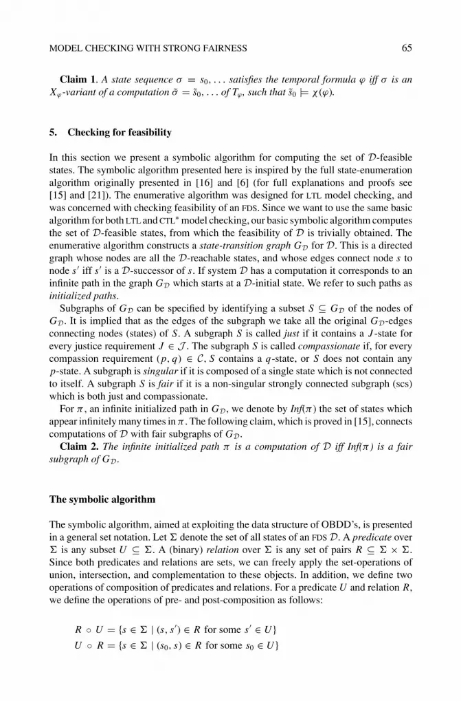
Claim 1. A state sequence σ = s0, . . . satisfies the temporal formula ϕ iff σ is anXϕ-variant of a computation σ = s0, . . . of Tϕ , such that s0 |= χ (ϕ).

5. Checking for feasibility

In this section we present a symbolic algorithm for computing the set of D-feasiblestates. The symbolic algorithm presented here is inspired by the full state-enumerationalgorithm originally presented in [16] and [6] (for full explanations and proofs see[15] and [21]). The enumerative algorithm was designed for LTL model checking, andwas concerned with checking feasibility of an FDS. Since we want to use the same basicalgorithm for both LTL and CTL∗ model checking, our basic symbolic algorithm computesthe set of D-feasible states, from which the feasibility of D is trivially obtained. Theenumerative algorithm constructs a state-transition graph GD for D. This is a directedgraph whose nodes are all the D-reachable states, and whose edges connect node s tonode s ′ iff s ′ is a D-successor of s. If system D has a computation it corresponds to aninfinite path in the graph GD which starts at a D-initial state. We refer to such paths asinitialized paths.

Subgraphs of GD can be specified by identifying a subset S ⊆ GD of the nodes ofGD. It is implied that as the edges of the subgraph we take all the original GD-edgesconnecting nodes (states) of S. A subgraph S is called just if it contains a J -state forevery justice requirement J ∈ J . The subgraph S is called compassionate if, for everycompassion requirement (p, q) ∈ C, S contains a q-state, or S does not contain anyp-state. A subgraph is singular if it is composed of a single state which is not connectedto itself. A subgraph S is fair if it is a non-singular strongly connected subgraph (scs)which is both just and compassionate.

For π , an infinite initialized path in GD, we denote by Inf(π ) the set of states whichappear infinitely many times in π . The following claim, which is proved in [15], connectscomputations of D with fair subgraphs of GD.

Claim 2. The infinite initialized path π is a computation of D iff Inf(π ) is a fairsubgraph of GD.

The symbolic algorithm

The symbolic algorithm, aimed at exploiting the data structure of OBDD’s, is presentedin a general set notation. Let � denote the set of all states of an FDS D. A predicate over� is any subset U ⊆ �. A (binary) relation over � is any set of pairs R ⊆ � × �.Since both predicates and relations are sets, we can freely apply the set-operations ofunion, intersection, and complementation to these objects. In addition, we define twooperations of composition of predicates and relations. For a predicate U and relation R,we define the operations of pre- and post-composition as follows:

R ◦ U = {s ∈ � | (s, s ′) ∈ R for some s ′ ∈ U }U ◦ R = {s ∈ � | (s0, s) ∈ R for some s0 ∈ U }

66 KESTEN ET AL.

If we view R as a transition relation, then R ◦ U is the set of all R-predecessors ofU -states, and U ◦ R is the set of all R-successors of U -states. To capture the set ofall states that can reach a U -state in a finite number of R-steps (including zero), wedefine

R∗ ◦ U = U ∪ R ◦ U ∪ R ◦ (R ◦ U ) ∪ R ◦ (R ◦ (R ◦ U )) ∪ · · · .

It is easy to see that R∗ ◦ U converges after a finite number of steps. In a similar way,we define

U ◦ R∗ = U ∪ U ◦ R ∪ (U ◦ R) ◦ R ∪ ((U ◦ R) ◦ R) ◦ R ∪ · · · ,

which captures the set of all states reachable in a finite number of R-steps from a U -state.For predicates U and W , we define the relation U × W as

U × W = {(s1, s2) ∈ �2 | s1 ∈ U, s2 ∈ W }.

Let D : 〈V, �, ρ,J , C〉, be an FDS. For an assertion ϕ over V , the system variablesof D, we denote by ||ϕ|| the predicate consisting of all states satisfying ϕ. Similarly, foran assertion ρ over (V, V ′), we denote by ||ρ|| the relation consisting of all state pairs〈s, s ′〉 satisfying ρ.

Algorithm FEASIBLE presented in figure 1, denotes by R the transition relation im-plied by ρ. The predicate variable new represents a set of states. We use the shorthandnotation

R ∩ newdef= R ∩ (new × �).

Algorithm FEASIBLE consists of a main loop which converges when the values of thepredicate variable new coincide on two successive visits to line 4. Prior to entry to the

Figure 1. Algorithm FEASIBLE.


main loop we compute in new the universal set of all reachable states in D and place inR the transition relation implied by ρ, restricted to pairs (s1, s2) where s1 is a reachablestate in D.

The main loop (lines 4–11), contains three inner loops. The inner loop at lines 6–7,successively removes from new all states which do not have a successor in new. Theloop at lines 8–9 removes from new all states which are not R∗-predecessors of someJ -state, for all justice requirements J ∈ J . The term R ∩new restricts R to pairs (s1, s2)where s1 is currently in new. This is done to avoid regeneration of states which havealready been eliminated. The loop at lines 10–11, removes from new all p-states whichare not R∗-predecessors of some q-state for some (p, q) ∈ C. The term R ∩new restrictsR again to pairs (s1, s2) where s1 is currently in new.

Finally, line 12 augments new with all its R∗-predecessors.

Correctness of the FEASIBLE Algorithm

The following sequence of claims establishes the correctness of the algorithm.

Claim 3 (Termination). Algorithm FEASIBLE terminates.

Proof: Let us denote by new4i the value of variable new on the i’th visit (i = 1, 2, . . .)

to line 4 of the algorithm. Since all assignments to variable new within the main loop, areof the form new := E where E ⊆ new, it is not difficult to see that new4

2 ⊆ new41. From

this, it can be established by induction on i that new4i+1, ⊆ new4

i , for every i = 1, 2 . . .. Itfollows that the sequence |new4

1| ≥ |new42| ≥ |new4

3| . . ., is a non-increasing sequence ofnatural numbers which must eventually stabilize. At the point of stabilization, we havethat new4

i+1 = new4i , implying termination of the algorithm.

Let D : 〈V, �, ρ,J , C〉 be an FDS, s be a D-reachable state and U be the set of statesresulting from the application of algorithm FEASIBLE to D.

Claim 4 (Completeness). If s is D-feasible then s ∈ U .

Proof: Assume that s is D-feasible. Then by definition, s is on an initialized fair pathπ in D, From Claim 2, Inf (π ) is a fair subgraph S ⊆ GD. Namely, S is a non-singularstrongly-connected subgraph (scs) which contains a J -state for every J ∈ J , and suchthat, for every (p, q) ∈ C, S contains a q-state or contains no p-state. Let

S : S ∪ {s ′|s ′ is on an initialized path to a state in S}

Obviously s ∈ S. Following the operations performed by algorithm FEASIBLE, we canshow that S is contained in the set new at all locations beyond the first visit to line 4.This is because any removal of states from new which is carried out in lines 7, 9, and11, cannot remove any state of S. Consequently, S must remain throughout the processand will be contained in U . Finally, when line 12 is executed, the set new is augmentedfrom S to S, implying that s ∈ U .

68 KESTEN ET AL.

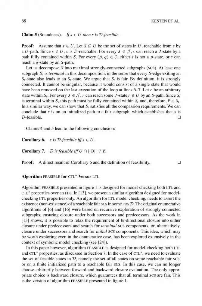
Claim 5 (Soundness). If s ∈ U then s is D-feasible.

Proof: Assume that s ∈ U . Let S ⊆ U be the set of states in U , reachable from s bya U -path. Since s ∈ U , s is D-reachable. For every J ∈ J , s can reach a J -state by apath fully contained within S. For every (p, q) ∈ C, either s is not a p-state, or s canreach a q-state by an S-path.

Let us decompose S into maximal strongly-connected subgraphs (SCS). At least onesubgraph St is terminal in this decomposition, in the sense that every S-edge exiting anSt -state also leads to an St -state. We argue that St is fair. By definition, it is stronglyconnected. It cannot be singular, because it would consist of a single state that wouldhave been removed on the last execution of the loop at lines 6–7. Let r be an arbitrarystate within St . For every J ∈ J , r can reach some J -state r ∈ U by an S-path. Since St

is terminal within S, this path must be fully contained within St and, therefore, r ∈ St .In a similar way, we can show that St satisfies all the compassion requirements. We canconclude that s is on an initialized path to a fair subgraph, which establishes that s isD-feasible.

Claims 4 and 5 lead to the following conclusion:

Corollary 6. s is D-feasible iff s ∈ U.

Corollary 7. D is feasible iff U ∩ ||�|| �= ∅.

Proof: A direct result of Corollary 6 and the definition of feasibility.

Algorithm FEASIBLE for CTL∗ Versus LTL

Algorithm FEASIBLE presented in figure 1 is designed for model-checking both LTL andCTL∗ properties over an FDS. In [13], we present a similar algorithm designed for model-checking LTL properties only. An algorithm for LTL model checking, needs to assert theexistence (non-existence) of a reachable fair SCS in some FDSD. The original enumerativealgorithms of [6] and [16] were based on recursive exploration of strongly connectedsubgraphs, ensuring closure under both successors and predecessors. As the work in[13] shows, it is possible to relax the requirement of bi-directional closure into eitherclosure under predecessors and search for terminal SCS components, or, alternatively,closure under successors and search for initial SCS components. This idea, which maybe worth exploring even in the enumerative case, has been explored extensively in thecontext of symbolic model checking (see [24]).

In this paper however, algorithm FEASIBLE is designed for model-checking both LTL

and CTL∗ properties, as discussed in Section 7. In the case of CTL∗, we need to evaluatethe set of feasible states in D, namely the set of all states on some reachable fair SCS,or on a finite initialized path to a reachable fair SCS. In this case, we can no longerchoose arbitrarily between forward and backward closure evaluation. The only appro-priate choice is backward closure, which guarantees that all terminal SCS are fair. Thisis the version of algorithm FEASIBLE presented in figure 1.


Model Checking LTL Properties

Using algorithm FEASIBLE, we can now model check an LTL property ϕ over an FDS Das follows.

• Construct the tester T¬ϕ .• Construct the synchronous parallel composition A : D|||T¬ϕ .

Let �A be the initial condition of the FDS A.• Evaluate FEASIBLE (D|||T¬ϕ) ∩ ||�A ∧ χ (¬ϕ)||.

The verification is based on the following Claim.

Claim 8 D |= ϕ iff FEASIBLE (D|||T¬ϕ) ∩ ||�A ∧ χ (¬ϕ)|| = ∅

The proof of equivalent claims can be found in [16, 26].

6. Extracting a witness

To use formal verification as an effective debugging tool in the context of verificationof finite-state reactive systems checked against temporal properties, a most useful infor-mation is a computation of the system which violates the requirement, to which we referas a witness or a counter-example. Since we reduced the problem of checking D |= ϕ

to checking the feasibility of D|||T¬ϕ , such a witness can be provided by a computationof the combined FDS D|||T¬ϕ .

In the following we present an algorithm which produces a computation of an FDS

that has been declared feasible. We introduce the list data structure to represent a linearlist of states. We use to denote the empty list. For two lists L1 = (s1, . . . , sa) andL2 = (sb, . . . , sc), we denote by L1 ∗ L2 their concatenation, defined by L1 ∗ L2 =(s1, . . . , sa, sb, . . . , sc). For a non-empty predicate U ⊆ �, we denote by choose(U ) aconsistent choice of one of the members of U .

The function path(source, destination, R), presented in figure 2, returns a list whichcontains the shortest R-path from a state in source to a state in destination. In the case thatsource and destination have a non-empty intersection, path will return a state belongingto this intersection which can be viewed as a path of length zero.

Finally, in figure 3 we present an algorithm which produces a computation of a givenFDS. Although a computation is an infinite sequence of states, if D is feasible, it alwayshas an ultimately periodic computation of the following form:

σ : s0, s1, . . . , sk,︸︷︷︸prefix

sk+1, . . . , sk,︸︷︷︸period

sk+1, . . . , sk,︸︷︷︸period

. . . , sk+1, . . . , sk,︸︷︷︸period

. . .

Based on this observation, our witness extracting algorithm will return as result the twofinite sequences prefix and period.

70 KESTEN ET AL.

Figure 2. Function path.

Figure 3. Algorithm WITNESS.


The algorithm starts by checking whether FDS D is feasible. It uses Algorithm FEA-SIBLE to perform this check. If D is found to be infeasible, the algorithm exits whileproviding a pair of empty lists as a result.

If D is found to be feasible, we store in final the set of states returned by FEASIBLE.This set contains the set of all states participating in a computation of D. We restrict thetransition relation R to pairs (s1, s2) where both s1 and s2 are states within final. Next, weperform a search for a terminal maximal strongly connected subgraph (terminal MSCS)within final. The search starts at s ∈ final, an arbitrarily chosen state within final. Inthe loop at lines 5 and 6 we search for a state s satisfying {s} ◦ R∗ ⊆ R∗ ◦ {s}. i.e. astate all of whose R∗-successors are also R∗-predecessors. This is done by successivelyreplacing s by a state s ∈ {s} ◦ R∗ − R∗ ◦ {s}, as long as the set of s-successors is notcontained in the set of s-predecessors. Eventually, execution of the loop must terminatewhen s reaches a terminal MSCS within final. Termination is guaranteed because eachsuch replacement moves the state from one MSCS to a proceeding MSCS in the canonicaldecomposition of final into MSCS’s.

A central point in the proof of correctness of Algorithm FEASIBLE established that anyterminal MSCS within final is a fair subgraph. Line 7 computes the MSCS containing sand assigns it to the variable final, while line 8 restricts the transition relation R to edgesconnecting states within final. Line 9 draws a (shortest) path from an initial state to thesubgraph final.

Lines 10–17 construct in period a traversing path, starting at the last state of the prefix,last (prefix), and returning to the same state, while visiting on the way states that ensurethat an infinite repetition of the period will fulfill all the fairness requirements.

Lines 11–13 ensure that period contains a J -state, for each J ∈ J . To preventunnecessary visits to states, we extend the path to visit the next J -state only if thepart of period that has already been constructed did not visit any J -state. Lines 14–16similarly take care of compassion. Here we extend the path to visit a q-state only ifthe constructed path did not already do so and the MSCS final contains some p-state.Finally, in line 17, we complete the path to form a closed cycle by looping back tolast(prefix).

7. Symbolic model checking CTL∗ properties

In the following, we show that algorithm FEASIBLE can be used to model check anarbitrary CTL∗ formula over a finite state FDS, taking weak and strong fairness constraintsinto consideration. We define CTL∗ with both future and past temporal operators. Wedenote the fragment of CTL∗ without the past operators as the future fragment of CTL∗.

An enumerative algorithm for model checking the future fragment of CTL∗ is presentedin [6]. In this work, Emerson and Lei show that model checking a CTL∗ formula overa finite state system, can be performed by recursive calls to an LTL model checker. Wetake a similar approach, using algorithm FEASIBLE to verify an arbitrary CTL∗ formulaover a finite state FDS D.

In the following, we first present the syntax and semantics of the logic, then discussthe use of algorithm FEASIBLE for verifying CTL∗ properties.

72 KESTEN ET AL.

7.1. The Logic CTL∗

A propositional CTL∗ formula is constructed out of propositions to which we apply theboolean operators, temporal operators and path quantifiers. The temporal operators arethe same operators presented in Section 3 for LTL. The path quantifiers are E f and A f ,as defined below.

A CTL∗ formula p is interpreted over the state graph (Kripke structure) generated byan FDS D. In the following, we use the term path in D as synonymous to a computationof D.

There are two types of formulas in CTL∗: State formulas which are interpreted overstates and path formulas which are interpreted over paths. Let P be a finite set ofpropositions. The syntax of a CTL∗ formula is defined inductively as follows.

State formulas:

• Every proposition p ∈ P is a state formula.• If p is a path formula, then E f p and A f p are state formulas.• If p and q are state formulas then so are ¬p and p ∨ q.

Path formulas:

• Every state formula is a path formula.• If p and q are path formulas then so are ¬p, p ∨ q, ©p, pUq, �p and pSq.

The formulas of CTL∗ are all the state formulas generated by the above rules.A state formula of the form Qp, where Q is a path quantifier and p is a path formula

containing no path quantifiers is called a basic state formula. A basic state formula ofthe form A f ψ(E f ψ) is called a basic universal (existential) formula. Note that the set ofbasic universal formulas corresponds to the set of linear temporal logic formulas (LTL).

The semantics of a CTL∗ formula is defined inductively as follows. State formulas areinterpreted over states in D. We define the notion of a path formula p holding at a states in D, denoted (D, s) |= p, as follows:

• For an assertion p• (D, s) |= p, ⇔ s |= p• (D, s) |= ¬p ⇔ (D, s) �|= p• (D, s) |= p ∨ q ⇔ (D, s) |= p or (D, s) |= q• (D, s) |= E f p ⇔ (D, π, j) |= p for some path π = π0, π1 . . . ∈ Comp(D), and

position j ≥ 0 satisfying π j = s.

The universal path quantifier is defined by A f p = ¬E f ¬p. Note that we have onlydefined the fair versions A f and E f of the path quantifiers. If one wants to verify aformula Aϕ over an FDS D, it can be done by verifying A f ϕ over Dunfair, which isobtained from D by removing all fairness requirements.

Path formulas are interpreted over a path (computation) inD. We define the notion of apath formula p holding at position j ≥ 0 of a path π inComp(D), denoted (D, π, j) |= p,


as follows:

• For a state formula p,(D, π, j) |= p⇔ (D, s) |= p, for s = π j

• (D, π, j) |= ¬p ⇔ (D, π, j) �|= p• (D, π, j) |= p ∨ q ⇔ (D, π, j) |= p or (D, π, j) |= q• (D, π, j) |= ©p ⇔ (D, π, j + 1) |= p• (D, π, j) |= pUq ⇔ (D, π, k) |= q for some k ≥ j and (D, π, i) |= p for every

i, j ≤ i < k• (D, π, j) |= �p ⇔ j > 0 and (D, π, j − 1) |= p• (D, π, j) |= pSq ⇔ (D, π, k) |= q for some k, 0 ≤ k ≤ j and (D, π, i) |= p for

every i, k < i ≤ j

Let p be a CTL∗ formula. We say that p holds on D (p is D-valid), denoted D |= p, if(D, s) |= p, for every initial state s in D. A CTL∗ formula p is called satisfiable if itholds on some model D. A CTL∗ formula is called valid if it holds on all models. Letp and q be CTL∗ formulas. We use the notations p ⇔ q and p ⇔ q as a shorthand forA f � (p → q) and A f � (p ↔ q) respectively.

7.2. Model checking basic state formulas

In the following we show how to model check basic state formulas over an FDS D.Algorithm FEASIBLE is formulated in set-theoretic terms. However, its implementation

obviously represents any set of states by a BDD which also represents an assertion. Inthe following we use notations such as ‖α‖ = FEASIBLE (D) in order to refer to theassertion α characterizing the set of states returned by the algorithm.

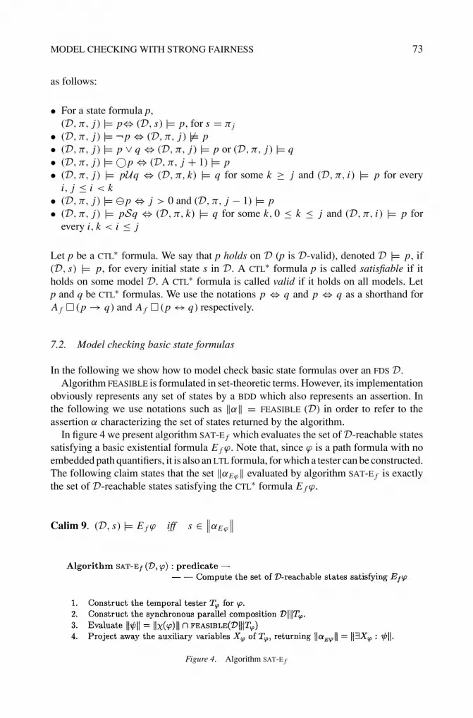
In figure 4 we present algorithm SAT-E f which evaluates the set of D-reachable statessatisfying a basic existential formula E f ϕ. Note that, since ϕ is a path formula with noembedded path quantifiers, it is also an LTL formula, for which a tester can be constructed.The following claim states that the set ‖αEϕ‖ evaluated by algorithm SAT-E f is exactlythe set of D-reachable states satisfying the CTL∗ formula E f ϕ.

Calim 9. (D, s) |= E f ϕ iff s ∈ ∥∥αE ϕ

∥∥

Figure 4. Algorithm SAT-E f

74 KESTEN ET AL.

Figure 5. Algorithm SAT-A f .

Corollary 10. D |= αE ϕ ⇔ E f ϕ

LetD be an FDS and A f ϕ be a basic universal formula. To evaluate the set ofD-reachablestates satisfying the formula, we use the CTL∗ congruence A f ϕ ⇔ ¬E f ¬ϕ.In figure 5 we present algorithm SAT-A f which evaluates the set of D-reachable statessatisfying a basic universal formula A f ϕ

The following claim states that the set ‖αAϕ‖ evaluated by algorithm SAT-A f is exactlythe set of D-reachable states satisfying the CTL∗ formula A f ϕ.

Claim 11. (D, s) |= A f ϕ iff s ∈ ‖αAϕ‖

Corollary 12. D |= αAϕ ⇔ A f ϕ

The two algorithms SAT-E f and SAT-A f can be combined into a single algorithm SAT-BASIC (D, ϕ), defined by

SAT-BASIC (D, E f ϕ) = SAT-E f (D, ϕ)

SAT-BASIC (D, A f ϕ) = SAT-A f (D, ϕ)

7.3. Decomposing an arbitrary CTL∗ formula into basic formulas

Consider an arbitrary (non basic) CTL∗ formula p which we wish to verify over an FDS

D. Following [6], we reduce the task of verifying formula p into simpler subtasks, eachrequired to verify a basic state formula over D.

In figure 6 we present algorithm VALID-CTL∗ for the verification of an arbitrary CTL∗

formula ψ over an FDS D. The algorithm consists of a while loop, where at each iterationof the loop formula ψ is reduced to a new formula in which all occurrences of somebasic state formula ϕ within ψ , are replaced by an assertion congruent to ϕ. The loopterminates when ψ is reduced to an assertion ψ that characterizes the set of states in Dsatisfying ψ . Formula ψ is D-valid if ‖�D ⊆ ‖ψ‖ or equivalently ‖�D‖ → ψ . Thefollowing claim states the soundness of algorithm VALID-CTL∗.


Figure 6. Algorithm VALID-CTL∗.

Figure 7. An example system D.

Let D be an FDS and ψ be an arbitrary CTL∗ formula, then

Claim 13. D |= ψ iff VALID-CTL∗ (D, ψ) returns T.

Example. Consider the system D presented in figure 7. This system has a single statevariable x and no fairness requirements. For this system we wish to prove the propertyf : E f E f �(x = 1), claiming the existence of a computation from each of whosestates it is possible to reach a state at which x = 1.

Using algorithm VALID-CTL∗, the task of verifying the non-basic formula

E f E f �(x = 1)

is reduced into the following tasks:

R1. Evaluate ‖α1‖ = SAT-BASIC (D, E f � (x = 1)). This yields α1 : (x = 0).R2. Evaluate ‖α2‖ = SAT-BASIC (D, E f α1). This yields α2 : (x = 0).R3. Evaluate �D → α2. This yields T.

8. Experimental results

The algorithms described in this paper were implemented within the TLV system [22].In the following section, we summarize our experimental results for algorithm FEASIBLE.

76 KESTEN ET AL.

The experiments were carried on a Sun Ultra with 1 Gigabyte of memory. We limit ourattention to LTL properties since our intention is to test the performance of algorithmFEASIBLE, which is the same for LTL and CTL∗.

8.1. Compassion at the algorithmic level

In order to test whether compassion at the algorithmic level yields better performance,we verify several examples which require compassion, using three different verificationmethods:

1. Verifying compassion at the algorithmic level. We denote this methods by NT (notransformation).

2. Transforming compassion to justice. From an automata theoretic perspective thistransforms a Streett automata into a Buchi automata. We denote this method by CJ

(compassion transformed to justice).3. Replacing compassion requirements in the system by adding an antecedent to the

verified property. We denote this method by CA (compassion as antecedent).

In method CJ, every compassion requirement is transformed into a justice requirement,at the price of introducing an extra boolean variable. Let D : 〈V, �, ρ,J , C〉 be an FDS.For every 〈pi , qi 〉 ∈ C we introduce a new variable ri and modify D as follows:

V : V ∪ {ri }� : � ∧ (ri = F)ρ : ρ ∧ (ri → (¬pi ∧ r ′

i ))J : J ∪ {(ri ∨ qi )}C : C − {(pi , qi )}

Method CA replaces a set of compassion requirements by a conjunction of LTL formulas,added as an antecedent to the verified property. Let D be an FDS, ϕ be a formula wewish to verify over D and C be the set of compassion requirements in D. We replace theverification of D |= ϕ by the following verification task:

D(−C) |=( ∧

〈p,q〉∈C

( � p → � q)

)→ ϕ

where D(−c) is the FDS D from which all the compassion requirements have beenremoved.

Note that a similar method can be applied to CTL∗ formulas. Let ψ be a CTL∗ property,and c be defined as follows:

c =∧

〈p,q〉∈C

( � p → � q)


We modify the calls to SAT-EF and SAT-A f in algorithm VALID-CTL∗ as follows:

• For a basic existential formula, call SAT-E f (D(−C), c ∧ ϕ).• For a basic universal formula, call SAT-A f (D(−C), c → ϕ).

8.1.1. Feasibility of parameterized programs. The programs we use for experimenta-tion are parameterized programs, of the form

S(n) : P[1]‖P[2]‖ . . . ||P[n]

which are verified for different values of n.Consider program DINE presented in figure 8. This program is a symmetric solution to

the dining philosophers problem, using semaphores for coordination between processes.Program DINE satisfies the safety requirement of mutual exclusion, stating that noneighboring philosophers can dine at the same time. However, this program fails tosatisfy the liveness requirement of accessibility for the first process, stating that if thephilosopher wishes to dine, it will eventually do so, as specified by:

ψ1 : �(at �2[1] → �at �4[1])

Program DINE is written in SPL (Simple Programming Language). The process oftranslating an SPL program to an FDS can be done automatically [21]. The translationassociates a compassion requirement with every request statement. The execution ofthe statement request s reduces the value of the semaphore s by 1. The statement can beexecuted only if s > 1. For example, the compassion requirement associated with �2 ofprocess 1 is 〈at �2[1] ∧ c[1] = 1, at �3[1]〉. This requirement ensures that if statement�2 is infinitely often enabled, it is infinitely often taken.

The non-critical statement has no corresponding justice or compassion requirement.A process may remain indefinitely in such a statement. For all other statements, the trans-lation associates a justice requirement of the form ¬ at �i . In program DINE, statements�0, �4, �5 and �6 each have corresponding justice requirements.

Note that it may be possible to translate an SPL program to an FDS using fewer justicerequirements, however, this typically requires a deeper understanding of the program,and thus manual translation.

Figure 8. Program DINE: The dining philosophers.

78 KESTEN ET AL.

Figure 9. Program MUX-SEM: Mutual exclusion with semaphores.

As a second example we consider the asymmetric version of the dining philosophers,program DINE-CONTR (dining philosophers with one contrary process), where the be-havior of one of the philosophers is reversed, i.e. it first lifts the right fork and then theleft one. The accessibility property ψ1 is valid for program DINE-CONTR.

The third example is program MUX-SEM, presented in figure 9. It implements mutualexclusion by semaphores. The following accessibility property is valid for programMUX-SEM:

ψ2 : (at �2[1] → � at �3[1])

In the following experiments we verify the accessibility property ψ1 for programDINE (Table 1) and DINE-CONTR (Table 2), and the accessibility property ψ2 for programMUX-SEM (Table 3 and figure 10).

In the tables summarizing our results, we use the following notations:

• n—The number of processes for which the parameterized program has been tested.• Proc.—The verification method used for the compassion requirements.• |J |, |C|—The number of justice and compassion requirements in the FDS D|||T¬ϕ .• Time—Timing results (in seconds).• BDD Peak—the maximum number of allocated BDD nodes.• Op.—The number of pre-composition (pre-image) operations invoked by algorithm

FEASIBLE.

Table 1. Program DINE.

n Proc. |J | |C| Time BDD Peak Op. Ext. Iter.

3 NT 14 6 0.49 10016 474 4

CJ 20 0 5.34 42674 711 5

CA 37 0 36.79 414467 1793 4

4 NT 18 8 3.54 17146 1007 6

CJ 26 0 148.02 223395 1079 5

CA 49 0 3829.80 2769339 2849 4


Table 2. Program DINE-CONTR.


3 NT 14 6 0.98 10016 991 10

CJ 20 0 2.74 36687 382 5

CA 37 0 19.40 334345 985 4

4 NT 18 8 3.63 21112 1119 9

CJ 26 0 29.11 135478 693 6

CA 49 0 1670.29 2066671 1567 4

5 NT 22 10 20.72 38222 1887 11

CJ 32 0 1262.11 241312 1238 7

CA – – – – – –

6 NT 26 12 126.32 87723 2888 13

CJ – – – – – –

CA – – – – – –

Table 3. Program MUX-SEM.


3 NT 11 3 0.09 5007 168 5

CJ 14 0 0.23 10002 162 5

CA 22 0 0.67 22805 184 3

4 NT 14 4 0.16 8726 204 5

CJ 18 0 0.59 14574 198 5

CA 29 0 4.40 98191 287 3

5 NT 17 5 0.26 10000 240 5

CJ 22 0 1.08 21202 234 5

CA 36 0 61.11 336517 405 3

6 NT 20 6 0.41 10051 276 5

CJ 26 0 1.80 30369 270 5

CA 43 0 1296.68 1070510 540 3

• Ext. Iter.—The number of external while-loop iterations performed (lines 4–11 ofalgorithm FEASIBLE).

Rows with no data are of experiments which did not terminate within one hour.The overall numbers of fairness requirements |J | + |C| of the NT and CJ methods are

equal, but the compassion requirements of method NT have been transformed to justicerequirements in method CJ. The additional justice requirements in method CA are due tothe tester, which is generated from a more complex property.

In all our experiments on real systems, method NT has the best results and methodCA has (by far) the worst results, both in execution time, and memory consumption.

80 KESTEN ET AL.

Figure 10. Program MUX-SEM: comparing NT and CJ for larger values of n.

However, in some cases the number of pre-composition operations for method CJ wasless than that of method NT.

8.1.2. Feasibility of randomly generated graphs. The experiments for real systemswere not conclusive with regard to the comparison between methods NT and CJ. Althoughmethod NT has better performance than CJ, the latter sometimes requires significantlyfewer pre-composition operations. In this section we present additional experiments forcomparing between the two methods.

We can view a system as a digraph where the state space of the system correspondsto the vertex space, and there is a directed edge from u to v in the digraph iff there is atransition from u to v in the system.

The problem in performing experiments over any set of real examples is that theyprovide a limited range of digraph patterns. Our experiments should not be biasedtowards any specific design. Therefore, we performed numerous experiments on randomdigraphs.

On the other hand, using random graphs has disadvantages: this method might beunrealistic since random graphs do not faithfully represent actual programs. That is whywe use this method only to complement our experiments on real programs.

We generate random digraphs as suggested in [27]. Given a graph G with vertices Vand edges E, the order of G is n = |V | and the density of G is d = |E |/|V |.

In the following tables, n = 1000. Each table only changes one parameter, either thesize of the set of compassion requirements, or the density of the random graph. Eachtable entry is the average of 100 experiments.

Table 4 produces results similar to those obtained for real systems. The real sys-tems we checked were parameterized, with compassion requirements associated witheach process. Therefore, the number of compassion requirements increases togetherwith the number of processes. In method CJ, each requirement introduces an additionalvariable, which affects performance of pre-composition operations. Therefore, whenthe number of pre-composition operations is roughly the same, using method NT ispreferable.


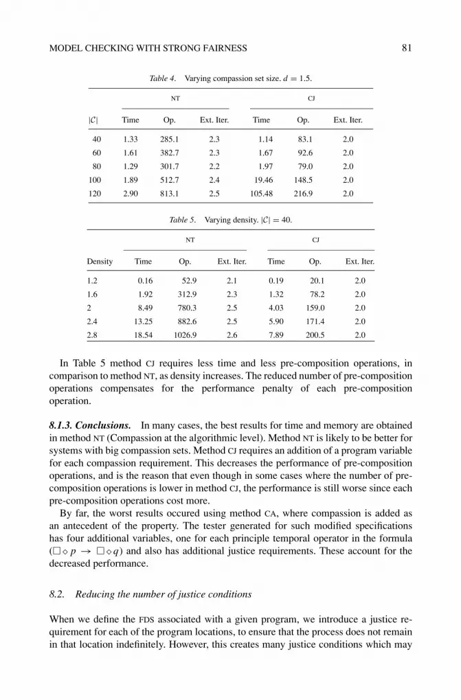
Table 4. Varying compassion set size. d = 1.5.

NT CJ

|C| Time Op. Ext. Iter. Time Op. Ext. Iter.

40 1.33 285.1 2.3 1.14 83.1 2.0

60 1.61 382.7 2.3 1.67 92.6 2.0

80 1.29 301.7 2.2 1.97 79.0 2.0

100 1.89 512.7 2.4 19.46 148.5 2.0

120 2.90 813.1 2.5 105.48 216.9 2.0

Table 5. Varying density. |C| = 40.

NT CJ

Density Time Op. Ext. Iter. Time Op. Ext. Iter.

1.2 0.16 52.9 2.1 0.19 20.1 2.0

1.6 1.92 312.9 2.3 1.32 78.2 2.0

2 8.49 780.3 2.5 4.03 159.0 2.0

2.4 13.25 882.6 2.5 5.90 171.4 2.0

2.8 18.54 1026.9 2.6 7.89 200.5 2.0

In Table 5 method CJ requires less time and less pre-composition operations, incomparison to method NT, as density increases. The reduced number of pre-compositionoperations compensates for the performance penalty of each pre-compositionoperation.

8.1.3. Conclusions. In many cases, the best results for time and memory are obtainedin method NT (Compassion at the algorithmic level). Method NT is likely to be better forsystems with big compassion sets. Method CJ requires an addition of a program variablefor each compassion requirement. This decreases the performance of pre-compositionoperations, and is the reason that even though in some cases where the number of pre-composition operations is lower in method CJ, the performance is still worse since eachpre-composition operations cost more.

By far, the worst results occured using method CA, where compassion is added asan antecedent of the property. The tester generated for such modified specificationshas four additional variables, one for each principle temporal operator in the formula(� � p → � � q) and also has additional justice requirements. These account for thedecreased performance.

8.2. Reducing the number of justice conditions

When we define the FDS associated with a given program, we introduce a justice re-quirement for each of the program locations, to ensure that the process does not remainin that location indefinitely. However, this creates many justice conditions which may

82 KESTEN ET AL.

Figure 11. Program CYCLE.

slow the algorithm down. In the following, we verify the effect of reducing the numberof justice requirements, on the performance of algorithm FEASIBLE.

Figure 11 presents a toy example designed to allow us to create an FDS which corre-sponds to the program, such that the number of justice requirements is greatly reducedwhen compared to the FDS which would normally be generated. Each process of programCYCLE may remain at location �1 indefinitely. However, once the process executes �1

it must not remain stuck in one of the other program locations, rather, it should cyclethrough the rest of the program locations until it returns to �1.

The idle statement makes a nondeterministic choice between either remaining foreverin the current program location, or advancing to the next statement. The skip statementdoes nothing except to advance to the next statement.

For each process i, program CYCLE has program locations �0, . . . , �m . The standardFDS corresponding to program CYCLE contains, for each process i and for each 0 ≤ j ≤m, j �= 1, a justice condition of the form ¬at � j . Therefore, a program of p processesand m locations in each process has p(m − 1) justice conditions. In the modified FDS

each process i has only a single justice condition:at �1.We verify the following accessibility property, for the first process:

ψ3 : �(at �2 → � at �m)

Tables 6 and 7 compare executions of programs with 6 and 10 program locations. Thesetables show a slight improvement when less justice conditions are generated. However,program CYCLE was tailored to simplify the reduction of justice conditions. In otherprograms we have checked, such as DINE, the price of reducing the number of justice

Table 6. Six Program Locations.

N 5 Justice Cond. 1 Justice Cond.

10 0.57 0.26

14 4.74 4.44

18 12.57 11.62

22 26.90 26.24

26 49.90 49.58

30 89.49 87.60


Table 7. Ten program locations.

N 9 Justice Cond. 1 Justice Cond.

6 0.81 0.23

8 4.26 3.26

10 10.44 9.11

12 21.05 18.79

14 38.66 35.74

16 64.68 60.94

conditions was either adding a single, complex justice requirement, or adding variables tothe verified system. In these cases, reducing the number of justice requirements increasedexecution time of the feasibility algorithm.

Note that for justice requirements of the form ¬at �i , line 9 of algorithm FEASIBLE

converges in only two steps. Although the standard, automatic way for generating anFDS from a program produces more justice requirements than what could optimally beproduced by hand, the price for processing each of these justice requirement is small.This can explain our experimental results.

We thus conclude that reducing the number of justice conditions is usually not rec-ommended.

References

1. J.R. Burch, E.M. Clarke, K.L. McMillan, D.L. Dill, and L.J. Hwang, “Symbolic model checking: 1020

states and beyond,” Inf. and Comp., Vol. 98, No. 2, pp. 142–170, 1992.2. E.M. Clarke and E.A. Emerson, “Design and synthesis of synchronization skeletons using branching time

temporal logic,” in Proc. IBM Workshop on Logics of Programs, Volume 131 of Lect. Notes in Comp.Sci., Springer-Verlag, 1981, pp. 52–71.

3. E.M. Clarke, O. Grumberg, and K. Hamaguchi, “Another look at LTL model checking,” Formal Methodsin System Design, Vol. 10, No. 1, 1997.

4. E.M. Clarke, O. Grumberg, D.E. Long, and X. Zhao, “Efficient generation of counterexamples andwitnesses in symbolic model checking,” in Proc. Design Automation Conference 95 (DAC95), 1995.

5. E.A. Emerson and C.L. Lei, “Efficient model-checking in fragments of the propositional modal μ-calculus,” in Proc. First IEEE Symp. Logic in Comp. Sci., pp. 267–278, 1986.

6. E.A. Emerson and C. Lei, “Modalities for model checking: Branching time logic strikes back,” Scienceof Computer Programming, Vol. 8, pp. 275–306, 1987.

7. N. Francez, Fairness, Springer-Verlag, 1986.8. D. Gabbay, A. Pnueli, S. Shelah, and J. Stavi, “On the temporal analysis of fairness,” in Proc. 7th ACM

Symp. Princ. of Prog. Lang., pp. 163–173, 1980.9. R.H. Hardin, R.P. Kurshan, S.K. Shukla, and M.Y. Vardi, “A new heuristic for bad cycle detection us-

ing BDDs,” in O. Grumberg and O. Grumberg (Eds.), Proc. 9th Intl. Conference on Computer AidedVerification, (CAV’97), Volume 1254 of Lect. Notes in Comp. Sci., Springer-Verlag, 1997, pp. 268–278.

10. M.R. Henzinger and J.A. Telle, “Faster algorithms for the nonemptiness of street automata and forcommunication protocol prunning,” in Proceedings of the 5th Scandina vian Workshop on AlgorithnTheory, 1996, pp. 10–20.

11. R. Hojati, H. Touati, R.P. Kurshan, and R.K. Brayton, “Efficient ω-regular language containment,” in G.V.Bochmann and D.K. Probst (Eds.), Proc. 4th Intl. Conference on Computer Aided Verification (CAV’92),

84 KESTEN ET AL.

Volume 697 of Lect. Notes in Comp. Sci., Springer-Verlag, number 663 in Lect. Notes in Comp. Sci.,SPringer-Verlag, 1992, pp. 396–409.

12. Y. Kesten and A. Pnueli, “Verification by augmented finitary abstraction, Inf. and Comp., Vol. 163, pp.203–243, 2000.

13. Y. Kesten, A. Pnueli, and L. Raviv, “Algorithmic verification of linear temporal logic specifications,” inK.G. Larsen, S. Skyum, and G. Winskel (Eds.), Proc, 25th Int. Col-loq. Aut. Lang. Prog., Volume 1443of Lect. Notes in Comp. Sci., Springer-Verlag, 1998, pp. 1–16.

14. R.P. Kurshan, Computer Aided Verification of Coordinating Processes, Princeton University Press, Prince-ton, New Jersey, 1995.

15. O. Lichtenstein, “Decidability, completeness, and extensions of linear time temporal logic,” PhD thesis,Weizmann Institute of Science, 1991.

16. O. Lichtenstein and A. Pnueli, “Checking that finite state concurrent programs satisfy their linear speci-fication,” in Proc. 12th ACM Symp. Princ. of Prog. Lang., 1985, pp. 97–107.

17. D. Lehmann, A. Pnueli, and J. Stavi, “Impartiality, justice and fairness: The ethics of concurrent termina-tion,” in Proc. 8th Int. Colloq. Aut. Lang. Prog., Volume 115 of Lect. Notes in Comp. Sci., Springer-Verlag,1981, pp. 264–277.

18. O. Lichtenstein, A. Pnueli, and L. Zuck, “The glory of the past,” in Proc. Conf. Logics of Programs,Volume 193 of Lect. Notes in Comp. Sci., Springer-Verlag, 1985, pp. 196–218.

19. Z. Manna and A. Pnueli, “Completing the temporal picture,” Theor. Comp. Sci., Vol. 83, No. 1, pp. 97–130,1991.

20. Z. Manna and A. Pnueli, Temporal Logic of Reactive and Concurrent Systems: Specification, Springer-Verlag, New York, 1991.

21. Z. Manna and A. Pnueli, Temporal Verification of Reactive Systems: Safety, Springer-Verlag, New York,1995.

22. A. Pnueli and E. Shahar, “A platform for combining deductive with algorithmic verification,” in R. Alur andT. Henzinger, R. Alur and T. Henzinger (Eds.), Proc. 8th Intl. Conference on Computer Aided Verification(CAV’96), Volume 1102 of Led. Notes in Comp. Sci., Springer- Verlag, 1996, pp. 184–195.

23. J.P. Queille and J. Sifakis, “Specification and verification of concurrent systems,” in cesar in M. Dezani-Ciancaglini and M. Montanari (Eds.), International Symposium on Programming, Volume 137 of Lect.Notes in Comp. Sci., Springer-Verlag, 1982, pp. 337–351.

24. K. Ravi, R. Bloem, and F. Somenzi, “A comparative study of symbolic algorithms for the computationof fair cycles,” in W.A. Hunt, Jr. and S.D. Johnson (Eds.), Formal Methods in Computer Aided Design,Volume 1954 of Lect. Notes in Comp. Sci., Springer-Verlag, 2000, pp. 143–160.

25. F.A. Stomp, W.-P. de Roever, and R.T. Gerth, “The μ-calculus as an assertion language for fairnessarguments,” Inf. and Comp., Vol. 82, pp. 278–322, 1989.

26. M.Y. Vardi and P. Wolper, “An automata-theoretic approach to automatic program verification,” in Proc.First IEEE Symp. Logic in Comp. Sci., 1986, pp. 332–344.

27. Z. Yang, “Performance analysis of symbolic reachability algorithms in model checking,” Master’s thesis,Rice University, 1999.

Documents

Model Checking with Strong Fairness