Embed Size (px)
Citation preview
01Tasmanian River Condition Index
Reference Manual


Executive Summary The Tasmanian River Condition Index (TRCI) is a framework for assessing the condition of Tasmanian river systems. It evaluates the condition of four key aspects of waterways: Aquatic Life, Hydrology, Physical Form and the Streamside Zone. These are known as sub-indices in the TRCI.
The TRCI is a practical tool to establish condition and monitor changes from this baseline into the future. It is a referential approach whereby the current condition of sites is compared with pre-European reference condition.
The TRCI is applicable state-wide and has been designed to be used by a range of organisations and groups. The whole TRCI, or selected sub-indices, may be used by the Tasmanian Natural Resource Management (NRM) regional organisations, State Government, Local Government, the community, industry and research organisations who require stream condition information.
The TRCI builds on existing assessment methods and brings new techniques to the field of stream condition assessment. The TRCI draws on information in the Tasmanian Conservation of Freshwater Ecosystem Values (CFEV) database and it is expected that the results will inform future versions of the database.
The TRCI can provide:
o a baseline assessment of condition from which changes can be monitored over time;
o an assessment of the effectiveness of natural resource management; o monitoring of the impacts of human activity in catchments on river systems (such as
water extraction and regulation, vegetation clearance, and instream structures); and o data for relevant information systems such as CFEV, the Tasmanian Vegetation
Monitoring and Mapping Program (TVMMP) and the Natural Values Atlas (NVA).
The TRCI can be used to inform:
o our understanding of the nature and condition of Tasmanian river systems; o prioritisation of investment and setting of strategic objectives; and o current and future State Government, Local Government and regional NRM
policies, planning, programs and initiatives for stream management and rehabilitation.
The TRCI has been developed in accordance with the National Framework for Assessment of River and Wetland Health (FARWH) to allow compatible reporting of the condition of Tasmanian river systems at the National level (Norris et al 2007).
A team of specialists in waterway condition and management, including consultants, academics and Tasmanian DPIW and NRM staff, developed and tested the TRCI
method over three years. The development of the TRCI was funded by the three Tasmanian Natural Resource Management regional bodies, the Tasmanian Government, the Australian Government and Hydro Tasmania. The project was managed by NRM South and Earth Tech Pty Ltd.
The manuals in the 2009 series This document is one of several volumes that describes the application of the Tasmanian River Condition Index (TRCI).
The Tasmanian River Condition Index Reference Manual (this document) describes why and how the TRCI was developed, application, sub-index methods and scoring;
The Tasmanian River Condition Index User’s and Field Manuals detail the procedures for the collection of field data for the Aquatic Life, Physical Form and Streamside Zone sub-indices; and describe the desktop assessment of the Hydrology sub-index:
o The Tasmanian River Condition Index Aquatic Life Field Manual (NRM South 2009a);
o The Tasmanian River Condition Index Hydrology User’s Manual (NRM South 2009b);
o The Tasmanian River Condition Index Physical Form Field Manual (NRM South 2009c); and
o The Tasmanian River Condition Index Streamside Zone Field Manual (NRM South 2009d).
These manuals are to be used in conjunction with the TRCI Reference Manual.
Several data analysis tools and a database to store TRCI data have also been developed. These are described in The Tasmanian River Condition Index Guide to Data Analysis Tools (NRM South 2009e). All TRCI products are available from NRM South.

Glossary Term Definition Abstraction The process of taking water from any source, either temporarily or permanently. Aggradation The raising of the level a steam bed by deposition of sediment. Algae Any of various chiefly aquatic, eukaryotic, photosynthetic organisms, ranging in
size from single-celled forms to the giant kelp. Algae were once considered to be plants but are now classified separately because they lack true roots, stems, leaves, and embryos.
Amplitude One half the full extent of a vibration, oscillation, or wave. Assessment Sites Sites within a river catchment at which data are recorded for the various sub-
indices. AusRivAS Australian River Assessment System, and Australian developed tool which uses
the macroinvertebrate community of a stream to assess its health. Average recurrence interval (ARI)
Long-term average interval of time within which an event will be equalled or exceeded. An example would be a flow event of a magnitude that has recurred 20 times in a 100 year period, this would have an ARI of 5 years.
Avulsion A temporally abrupt change in the course of a stream, resulting in the development of a new channel and the abandonment of an old channel.
Bankfull flow Maximum stream flow that can be accommodated within the channel without overtopping the banks and spreading onto the floodplain. Generally the level associated with two- or three-year stream flow events
Benthic Relating to the bottom of a water body (e.g. river, pond, sea or lake) or to the organisms (algae, macroinvertebrates) that live there.
CFEV Conservation of Freshwater Ecosystem Values database CFEV stream network
The 1:25 000 ‘river spatial data layer’ in CFEV, comprised of numerous river sections (reaches)
Coefficient of variation
A statistic, being the ratio of the standard deviation to the mean. Useful for comparing the degree of variation from one data series to another, even if the means are very different in magnitude.
Component A constituent element of one of the TRCI Sub-Indices eg the Hydrology Sub-index is itself comprised of 12 components.
Degradation The lowering of the level a steam bed by erosion of substrate or previously deposited sediment.
Diversion The taking of water from a stream or other body of water into a canal, pipe, or other conduit.
Event In hydrology, a term used for an occurrence such as a flood or a rainfall of particular intensity.
Exceedance flow The flow that is exceeded for a specified percentage of time eg the 50% exceedance flow is exceeded 50% of the time..
Flow (or Discharge) Total volume of water flowing past a point in a stream in a specified time interval. Thus, daily discharge is the volume within a specific 24 hour period, annual discharge the volume in a given year.
Flow duration curve A cumulative frequency curve that shows the percentage of time that specified discharges are equalled or exceeded. May be graphically represented by plotting the discharge on the Y axis against the percentage of time equalled or exceeded on the X axis.
Fish Any of numerous cold-blooded aquatic vertebrates of the superclass Pisces, characteristically having fins, gills, and a streamlined body
Geomorphology The study of the evolution and configuration of landforms. Hydrograph A graph showing stage or discharge of a stream over a time period. Hydrology Broadly, the study of the movement, distribution, and quality of water throughout
the Earth, from the moment of its precipitation until it is returned to the atmosphere through evapotranspiration or is discharged into the ocean.
Index Something that serves to guide, point out, or otherwise facilitate reference. The TRC Index serves as a guide to the condition of streams within Tasmania.
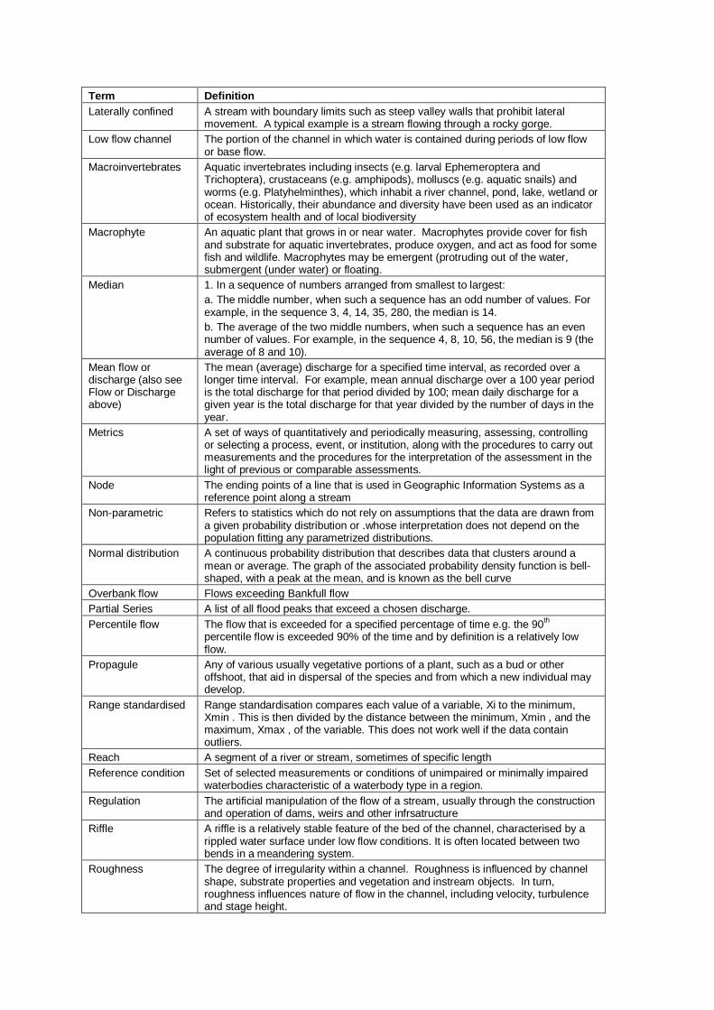
Term Definition Laterally confined A stream with boundary limits such as steep valley walls that prohibit lateral
movement. A typical example is a stream flowing through a rocky gorge. Low flow channel The portion of the channel in which water is contained during periods of low flow
or base flow. Macroinvertebrates Aquatic invertebrates including insects (e.g. larval Ephemeroptera and
Trichoptera), crustaceans (e.g. amphipods), molluscs (e.g. aquatic snails) and worms (e.g. Platyhelminthes), which inhabit a river channel, pond, lake, wetland or ocean. Historically, their abundance and diversity have been used as an indicator of ecosystem health and of local biodiversity
Macrophyte An aquatic plant that grows in or near water. Macrophytes provide cover for fish and substrate for aquatic invertebrates, produce oxygen, and act as food for some fish and wildlife. Macrophytes may be emergent (protruding out of the water, submergent (under water) or floating.
Median 1. In a sequence of numbers arranged from smallest to largest: a. The middle number, when such a sequence has an odd number of values. For example, in the sequence 3, 4, 14, 35, 280, the median is 14. b. The average of the two middle numbers, when such a sequence has an even number of values. For example, in the sequence 4, 8, 10, 56, the median is 9 (the average of 8 and 10).
Mean flow or discharge (also see Flow or Discharge above)
The mean (average) discharge for a specified time interval, as recorded over a longer time interval. For example, mean annual discharge over a 100 year period is the total discharge for that period divided by 100; mean daily discharge for a given year is the total discharge for that year divided by the number of days in the year.
Metrics A set of ways of quantitatively and periodically measuring, assessing, controlling or selecting a process, event, or institution, along with the procedures to carry out measurements and the procedures for the interpretation of the assessment in the light of previous or comparable assessments.
Node The ending points of a line that is used in Geographic Information Systems as a reference point along a stream
Non-parametric Refers to statistics which do not rely on assumptions that the data are drawn from a given probability distribution or .whose interpretation does not depend on the population fitting any parametrized distributions.
Normal distribution A continuous probability distribution that describes data that clusters around a mean or average. The graph of the associated probability density function is bell-shaped, with a peak at the mean, and is known as the bell curve
Overbank flow Flows exceeding Bankfull flow Partial Series A list of all flood peaks that exceed a chosen discharge. Percentile flow The flow that is exceeded for a specified percentage of time e.g. the 90th
percentile flow is exceeded 90% of the time and by definition is a relatively low flow.
Propagule Any of various usually vegetative portions of a plant, such as a bud or other offshoot, that aid in dispersal of the species and from which a new individual may develop.
Range standardised Range standardisation compares each value of a variable, Xi to the minimum, Xmin . This is then divided by the distance between the minimum, Xmin , and the maximum, Xmax , of the variable. This does not work well if the data contain outliers.
Reach A segment of a river or stream, sometimes of specific length Reference condition Set of selected measurements or conditions of unimpaired or minimally impaired
waterbodies characteristic of a waterbody type in a region. Regulation The artificial manipulation of the flow of a stream, usually through the construction
and operation of dams, weirs and other infrsatructure Riffle A riffle is a relatively stable feature of the bed of the channel, characterised by a
rippled water surface under low flow conditions. It is often located between two bends in a meandering system.
Roughness The degree of irregularity within a channel. Roughness is influenced by channel shape, substrate properties and vegetation and instream objects. In turn, roughness influences nature of flow in the channel, including velocity, turbulence and stage height.

Term Definition Spell A period of time Stage (Height) The height of a water surface above an established datum Stream A waterway of indeterminate size, includes rivers, creeks, rivulets Sub-index One of the four themes or subjects of investigation that together comprise the
TRCI. The four sub-indices are Aquatic Life, Hydrology, Streamside Zone and Physical Form.:
Valley An area of lowland between ranges of mountains, hills, or other uplands, Valley margin The edge of the valley, where the lowland area meets the hills, usually associated
with a notable change in slope. Wavelength The distance between repeating units of a propagating wave of a given frequency,
typically measured between peaks of the wave
Abbreviations CFEV - Conservation of Freshwater Ecosystem Values
DPIW - (Tasmanian) Department of Primary Industries and Water
FARWH - Framework for Assessment of River and Wetland Health
ISC - (Victorian) Index of Stream Condition
Km - kilometres
M - metres
NRM - Natural Resource Management
NVA - Natural Values Atlas
RARC - Rapid Appraisal of Riparian Condition
SRA - Sustainable Rivers Audit
TRCI - Tasmanian River Condition Index
TVMMP - Tasmanian Vegetation Monitoring and Mapping Program
VCA - Vegetation Condition Assessment
Contents 1 Introduction ...................................................................................................... 1
1.1 Purpose of the TRCI ........................................................................................... 1
1.2 Limitations of the TRCI ....................................................................................... 2
1.3 Why was the TRCI developed? .......................................................................... 2
1.4 How was the TRCI developed? .......................................................................... 5
1.5 How will the TRCI be applied? ............................................................................ 9
1.6 Anticipating future improvements in condition assessment ............................... 11
1.7 References - The Development of the TRCI ..................................................... 11
Appendix to Chapter 1: Further detail on the TRCI project .......................................... 15
2 Applying the TRCI .......................................................................................... 17
2.1 Defining objectives ........................................................................................... 17
2.2 Spatial scale and reporting units ....................................................................... 17
2.3 Which sub-indices to assess?........................................................................... 18
2.4 Number of sites and confidence required.......................................................... 19
2.5 Site selection .................................................................................................... 21
2.6 Recommended sampling strategy for the TRCI ................................................ 23
2.7 Field and desktop measurements and scoring .................................................. 24
2.8 Aggregation and interpretation of TRCI scores ................................................. 24
2.9 References - Applying the TRCI ....................................................................... 25
Appendix to Chapter 2: Further detail on TRCI sampling ............................................. 28
3 Aquatic Life Sub-Index ................................................................................... 37
3.1 Introduction ....................................................................................................... 37
3.2 Background, component selection and rationale............................................... 38
3.3 Aquatic Life reference conditions ...................................................................... 39
3.4 Description of components ............................................................................... 39
3.5 Procedure to evaluate the Aquatic Life sub-index ............................................. 43
3.6 Assessment methods and sample processing .................................................. 45
3.7 Scoring – Aquatic Life metrics, indicators and components .............................. 51
3.8 Scoring – Aquatic Life sub-index score for a site .............................................. 62
3.9 Scoring – Aquatic Life score for a reporting unit................................................ 64
3.10 Missing data ..................................................................................................... 64
3.11 Example applications of the Aquatic Life sub-index...........................................65
3.12 References - Aquatic Life ..................................................................................67
Appendix to Chapter 3: Further detail on the Aquatic Life sub-index ............................70
4 Hydrology Sub-Index ......................................................................................79
4.1 Introduction .......................................................................................................79
4.2 Background ......................................................................................................79
4.3 Component selection ........................................................................................80
4.4 Hydrological data ..............................................................................................85
4.5 Defining reference condition .............................................................................86
4.6 Description of components................................................................................86
4.7 Resources required...........................................................................................97
4.8 Scoring - Hydrology score at a node .................................................................97
4.9 Scoring – Hydrology score for a reporting unit ..................................................97
4.10 Missing data.................................................................................................... 101
4.11 References - Hydrology .................................................................................. 101
5 Physical Form Sub-Index ............................................................................. 103
5.1 Introduction ..................................................................................................... 103
5.2 Background and component selection ............................................................ 103
5.3 Physical Form reference conditions ................................................................ 104
5.4 A Physical Form Assessment Site .................................................................. 107
5.5 Description of components.............................................................................. 109
5.6 Summary of Assessment Procedure ............................................................... 117
5.7 Methods .......................................................................................................... 119
5.8 Scoring – Physical Form component and site scores ...................................... 120
5.9 Future assessments and the development of additional benchmarks.............. 122
5.10 References - Physical Form ............................................................................ 122
Appendix to Chapter 5: Further detail on the Physical Form sub-index ...................... 126
6 Streamside Zone Sub-Index ......................................................................... 197
6.1 Background, component selection and rationale ............................................. 197
6.2 Streamside Zone reference condition.............................................................. 199
6.3 Assessment site .............................................................................................. 202
6.4 Description of components.............................................................................. 203
6.5 Procedure to assess the Streamside Zone sub-index ..................................... 208
6.6 Scoring - Streamside Zone component and site scores .................................. 209
6.7 Scoring - Streamside Zone score for a reporting unit ...................................... 210
6.8 Missing data ................................................................................................... 211
6.9 Example application of Streamside Zone sub- index ...................................... 212
6.10 References - Streamside Zone ....................................................................... 214
Appendix to Chapter 6: Further detail on the Streamside Zone sub-index ................. 216
7 Water Quality Sub-Index .............................................................................. 247
7.1 Introduction ..................................................................................................... 247
7.2 Developing the Draft Method .......................................................................... 247
7.3 Status of the Water Quality sub-index ............................................................. 249
7.4 References - Water Quality ............................................................................ 250

Acknowledgements The TRCI method was developed and tested by a team of over 20 specialists and they are gratefully acknowledged.
Fiona Dyer and the expert panel provided valuable technical direction, insight and guidance throughout the development of the method. The working groups provided intellectual input to the sub-index methods, as well as the sampling strategy and database development. NRM representatives commented on draft reports and supported the project from its inception. Johanna Slijkerman skilfully managed the project team through each phase of the project.
A range of staff from the project team, DPIW Tasmania, NRM South, Cradle Coast NRM, Launceston Environment Centre, Hydro Tasmania, Greening Australia, Enviromon, Maunsell (formerly Earth Tech), Freshwater Systems and Todd Walsh assisted with field and desktop trials of the TRCI. Landholders who allowed staff access to waterways during the testing of the method are also acknowledged.
Special thanks to Paul Wilson and Sam Marwood from the Victorian Department of Sustainability and Environment for their support and advice throughout the project.
The efforts of the following individuals and organisations who assisted with the development of the TRCI are greatly appreciated:
Expert panel: Michael Askey-Doran Prof. Barry Hart
Dr Tony Ladson Dr Martin Read
NRM Representatives: Aniela Grun Alistair Kay Andrew Baldwin
James McKee Sue Botting Richard Ingram
Working groups: Adj. Prof. Peter Davies Prof. Richard Norris Dr Fiona Dyer Dr Michael Stewardson Glenn McDermott Bryce Graham Dr James Grove Ian Houshold Alexandra Spink
Assoc. Prof. Ian Rutherfurd Dr Amy Jansen Johanna Slijkerman James Kaye Dr Mick Brown Leanne Wilkinson Dr Richard Marchant Wayne Robinson Josh Hawkins Darren Smith

Other contributors: Kaylene Allan Chris Arnott Greg Carson Laurie Cook Monique Coze Nikki den Exter Sally Fenner Freshwater Systems staff Maxine Glass Shivaraj Gurung Ross Hardie Alison Howman
Vic Hughes Inland Fisheries Service staff Tegan Liston David Keast Dax Noble Debbie Searle Patrick Taylor Michelle Townsend Kane Travis Catherine Walsh Todd Walsh Amanda Wealands
The project was funded by the Australian and Tasmanian State Governments and managed by NRM South. Additional funding and in-kind support was provided by DPIW Tasmania and Hydro Tasmania.

Enquiries should be directed to:
NRM South ABN 867 040 886 98
313 Macquarie St PO Box 425 South Hobart TAS 7004
Phone: 03 6221 6111 Fax: 03 6221 6166
Web: www.nrmsouth.org.au Email: [email protected]
Tasmanian River Condition Index Reference Manual
1
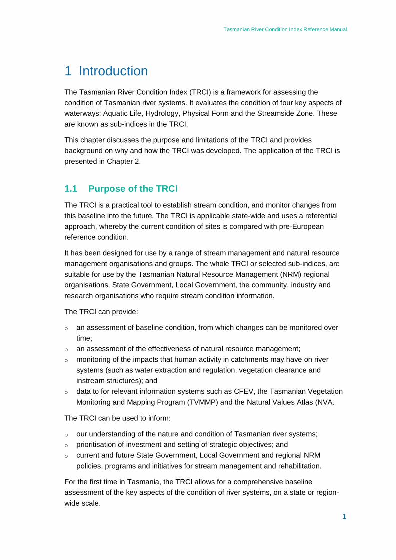
1 Introduction The Tasmanian River Condition Index (TRCI) is a framework for assessing the condition of Tasmanian river systems. It evaluates the condition of four key aspects of waterways: Aquatic Life, Hydrology, Physical Form and the Streamside Zone. These are known as sub-indices in the TRCI.
This chapter discusses the purpose and limitations of the TRCI and provides background on why and how the TRCI was developed. The application of the TRCI is presented in Chapter 2.
1.1 Purpose of the TRCI The TRCI is a practical tool to establish stream condition, and monitor changes from this baseline into the future. The TRCI is applicable state-wide and uses a referential approach, whereby the current condition of sites is compared with pre-European reference condition.
It has been designed for use by a range of stream management and natural resource management organisations and groups. The whole TRCI or selected sub-indices, are suitable for use by the Tasmanian Natural Resource Management (NRM) regional organisations, State Government, Local Government, the community, industry and research organisations who require stream condition information.
The TRCI can provide:
o an assessment of baseline condition, from which changes can be monitored over time;
o an assessment of the effectiveness of natural resource management; o monitoring of the impacts that human activity in catchments may have on river
systems (such as water extraction and regulation, vegetation clearance and instream structures); and
o data to for relevant information systems such as CFEV, the Tasmanian Vegetation Monitoring and Mapping Program (TVMMP) and the Natural Values Atlas (NVA.
The TRCI can be used to inform:
o our understanding of the nature and condition of Tasmanian river systems; o prioritisation of investment and setting of strategic objectives; and o current and future State Government, Local Government and regional NRM
policies, programs and initiatives for stream management and rehabilitation.
For the first time in Tasmania, the TRCI allows for a comprehensive baseline assessment of the key aspects of the condition of river systems, on a state or region-wide scale.

Tasmanian River Condition Index Reference Manual
2
The TRCI has been developed in accordance with the National Framework for Assessment of River and Wetland Health (FARWH) to allow compatible reporting of the condition of Tasmanian river systems at the National level (Norris et al, 2007).
1.2 Limitations of the TRCI The TRCI provides a broad scale, primarily reconnaissance, assessment of stream condition. It has been designed to measure changes caused by landscape scale activities. However, some components of the method may indicate changes at the site scale, or could be adapted for this purpose. The TRCI was not designed to provide a detailed inventory of the natural values, or for example, to investigate threatened species at a site or in a catchment.
The TRCI does not investigate causality per se. The results of the TRCI may trigger the need for a more detailed assessment into the causes of poor condition or a change in condition. Over time, TRCI results will assist in understanding the causes of change in condition but this is not the primary purpose of the method.
TRCI reference conditions are at a stage of development that reflects current data availability. It is hoped that as more data is collected, reference conditions will be further refined (Section 1.6.1).
1.3 Why was the TRCI developed? The TRCI was developed to provide an integrated method for the assessment and reporting of the condition of Tasmanian streams, that could be applied consistently across the state. The method was to be aligned with national protocols and recognised by the NRM regions and the State.
Prior to the development of the TRCI, assessments of stream condition in Tasmania were based on disparate programs and projects which generally targeted a single feature of stream condition, such as macroinvertebrates or physical form. Projects were completed by the State Government or other natural resource management groups. Techniques used were based on AUSRIVAS (Krasnicki et al. 2001) for the assessment of macroinvertebrates, Rivercare planning which involved assessments of vegetation, weeds, and used RiverStyles™ (Brierly and Fryirs 2005) for the physical condition of rivers. The ‘habitat hectares approach’ (Parkes et al 2003), the Vegetation Condition Assessment (VCA) method (Michaels 2006) or the Rapid Appraisal of Riparian Condition (RARC) (Jansen et al 2005) were used for the assessment of vegetation condition.
Elements of the 1999 Victorian Index of Stream Condition (ISC) (Ladson et al 1999) and Queensland’s 1993 Anderson method (Anderson 1993) were trialled from 1998 to 2003 in 11 Tasmanian catchments. This was known as the Index of River Condition
Tasmanian River Condition Index Reference Manual
3
(IRC) and outputs were used for State of the Rivers reporting. Users of the IRC suggested that this method was not entirely appropriate for Tasmanian conditions (Ladson and Grove 2006). Suggested improvements included:
o the streamside zone sub-index needed to be improved, particularly in areas of regrowth;
o the IRC would be strengthened by the addition of AUSRIVAS and fish information; o the Hydrology flow deviation indicator did not seem sensitive enough for Tasmanian
conditions; o the physical form indicators were too coarse and needed to be improved.
The need to update, consolidate and integrate all of these assessments into one broad framework was identified, and the development of the TRCI was commissioned. This framework was to incorporate improvements in stream condition assessment programs that had occurred nationally, and integrate with other tools in use in the State, such as the Conservation of Freshwater Ecosystem Values (CFEV) database. The TRCI approach was to be consistent with national protocols and be recognised by the NRM regions and the State. The framework was to assess the key elements of river condition through indicators such as fish, macro-invertebrates, algae, flow regimes, geomorphology and riparian vegetation. This philosophy is explained in more detail in the National Framework for Assessment of River and Wetland Health (FARWH) (Norris et al, 2007).
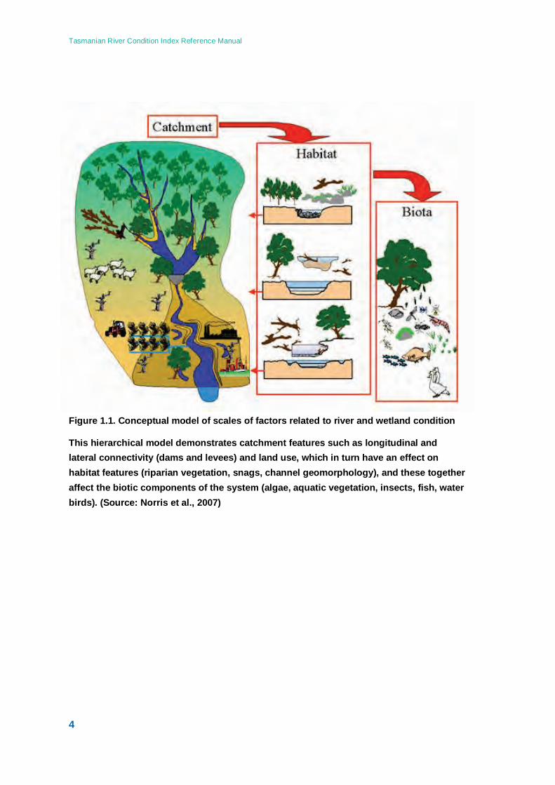
The FARWH suggests that the condition of a river can be defined by its aquatic life, hydrology, physical form, riparian vegetation and water quality. This approach is supported by the well accepted hierarchical model of river and wetland function (Figure 1.1) where broad-scale catchment characteristics affect local hydrology, hydraulics, habitat features, water and soil quality, which in turn, influence the river and biota (Norris et al, 2007). The FARWH conceptual model of scales of factors related to river and wetland condition is presented in Figure 1.1.
Tasmanian River Condition Index Reference Manual
4
Figure 1.1. Conceptual model of scales of factors related to river and wetland condition
This hierarchical model demonstrates catchment features such as longitudinal and lateral connectivity (dams and levees) and land use, which in turn have an effect on habitat features (riparian vegetation, snags, channel geomorphology), and these together affect the biotic components of the system (algae, aquatic vegetation, insects, fish, water birds). (Source: Norris et al., 2007)
Tasmanian River Condition Index Reference Manual
5
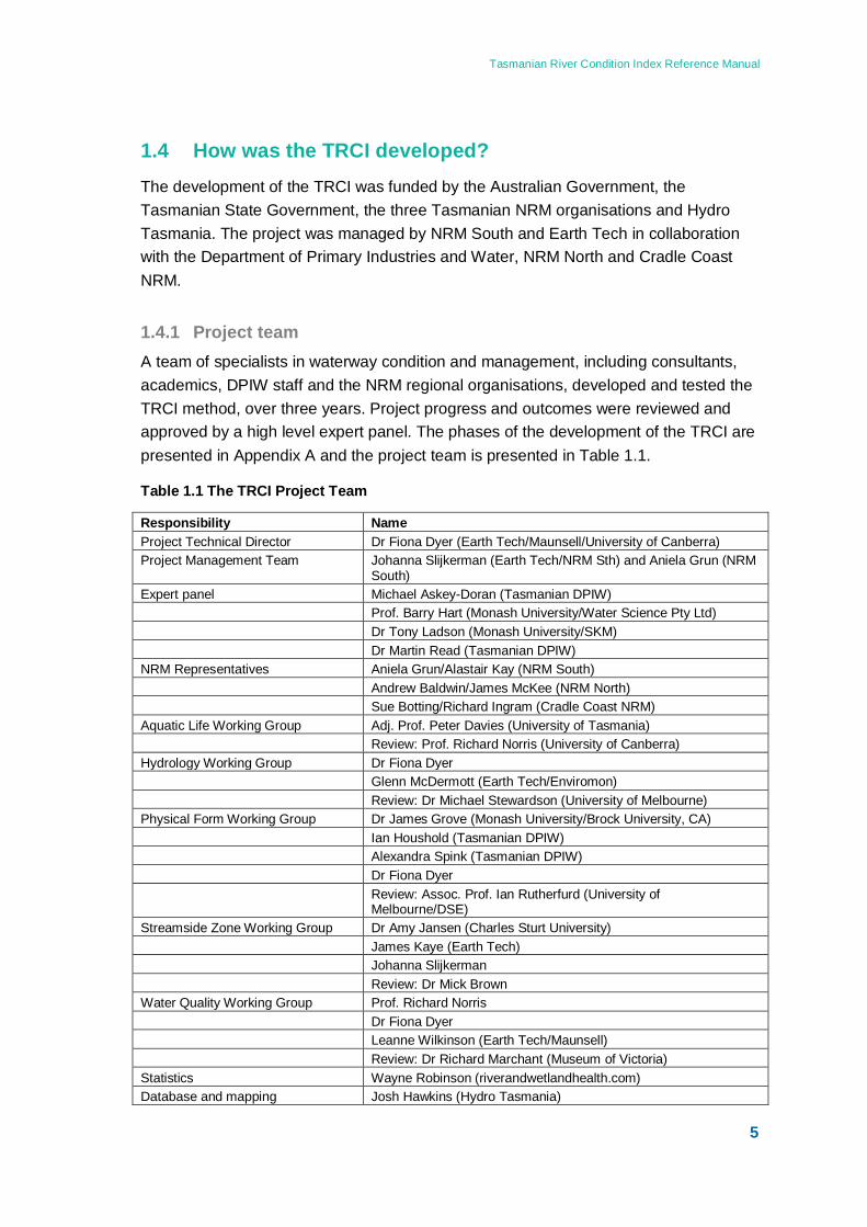
1.4 How was the TRCI developed? The development of the TRCI was funded by the Australian Government, the Tasmanian State Government, the three Tasmanian NRM organisations and Hydro Tasmania. The project was managed by NRM South and Earth Tech in collaboration with the Department of Primary Industries and Water, NRM North and Cradle Coast NRM.
1.4.1 Project team A team of specialists in waterway condition and management, including consultants, academics, DPIW staff and the NRM regional organisations, developed and tested the TRCI method, over three years. Project progress and outcomes were reviewed and approved by a high level expert panel. The phases of the development of the TRCI are presented in Appendix A and the project team is presented in Table 1.1.
Table 1.1 The TRCI Project Team
Responsibility Name Project Technical Director Dr Fiona Dyer (Earth Tech/Maunsell/University of Canberra) Project Management Team Johanna Slijkerman (Earth Tech/NRM Sth) and Aniela Grun (NRM
South) Expert panel Michael Askey-Doran (Tasmanian DPIW) Prof. Barry Hart (Monash University/Water Science Pty Ltd) Dr Tony Ladson (Monash University/SKM) Dr Martin Read (Tasmanian DPIW) NRM Representatives Aniela Grun/Alastair Kay (NRM South) Andrew Baldwin/James McKee (NRM North) Sue Botting/Richard Ingram (Cradle Coast NRM) Aquatic Life Working Group Adj. Prof. Peter Davies (University of Tasmania) Review: Prof. Richard Norris (University of Canberra) Hydrology Working Group Dr Fiona Dyer Glenn McDermott (Earth Tech/Enviromon) Review: Dr Michael Stewardson (University of Melbourne) Physical Form Working Group Dr James Grove (Monash University/Brock University, CA) Ian Houshold (Tasmanian DPIW) Alexandra Spink (Tasmanian DPIW) Dr Fiona Dyer Review: Assoc. Prof. Ian Rutherfurd (University of
Melbourne/DSE) Streamside Zone Working Group Dr Amy Jansen (Charles Sturt University) James Kaye (Earth Tech) Johanna Slijkerman Review: Dr Mick Brown Water Quality Working Group Prof. Richard Norris Dr Fiona Dyer Leanne Wilkinson (Earth Tech/Maunsell) Review: Dr Richard Marchant (Museum of Victoria) Statistics Wayne Robinson (riverandwetlandhealth.com) Database and mapping Josh Hawkins (Hydro Tasmania)
Tasmanian River Condition Index Reference Manual
6
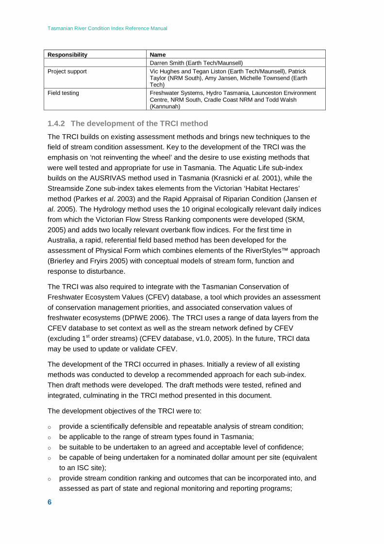
Responsibility Name Darren Smith (Earth Tech/Maunsell) Project support Vic Hughes and Tegan Liston (Earth Tech/Maunsell), Patrick
Taylor (NRM South), Amy Jansen, Michelle Townsend (Earth Tech)
Field testing Freshwater Systems, Hydro Tasmania, Launceston Environment Centre, NRM South, Cradle Coast NRM and Todd Walsh (Kannunah)
1.4.2 The development of the TRCI method The TRCI builds on existing assessment methods and brings new techniques to the field of stream condition assessment. Key to the development of the TRCI was the emphasis on ‘not reinventing the wheel’ and the desire to use existing methods that were well tested and appropriate for use in Tasmania. The Aquatic Life sub-index builds on the AUSRIVAS method used in Tasmania (Krasnicki et al. 2001), while the Streamside Zone sub-index takes elements from the Victorian ‘Habitat Hectares’ method (Parkes et al. 2003) and the Rapid Appraisal of Riparian Condition (Jansen et al. 2005). The Hydrology method uses the 10 original ecologically relevant daily indices from which the Victorian Flow Stress Ranking components were developed (SKM, 2005) and adds two locally relevant overbank flow indices. For the first time in Australia, a rapid, referential field based method has been developed for the assessment of Physical Form which combines elements of the RiverStyles™ approach (Brierley and Fryirs 2005) with conceptual models of stream form, function and response to disturbance.
The TRCI was also required to integrate with the Tasmanian Conservation of Freshwater Ecosystem Values (CFEV) database, a tool which provides an assessment of conservation management priorities, and associated conservation values of freshwater ecosystems (DPIWE 2006). The TRCI uses a range of data layers from the CFEV database to set context as well as the stream network defined by CFEV (excluding 1st order streams) (CFEV database, v1.0, 2005). In the future, TRCI data may be used to update or validate CFEV.
The development of the TRCI occurred in phases. Initially a review of all existing methods was conducted to develop a recommended approach for each sub-index. Then draft methods were developed. The draft methods were tested, refined and integrated, culminating in the TRCI method presented in this document.
The development objectives of the TRCI were to:
o provide a scientifically defensible and repeatable analysis of stream condition; o be applicable to the range of stream types found in Tasmania; o be suitable to be undertaken to an agreed and acceptable level of confidence; o be capable of being undertaken for a nominated dollar amount per site (equivalent
to an ISC site); o provide stream condition ranking and outcomes that can be incorporated into, and
assessed as part of state and regional monitoring and reporting programs;
Tasmanian River Condition Index Reference Manual
7
o provide an indication of the health of the whole of river systems, providing an informed platform from which priorities for management and rehabilitation can be identified and implemented.
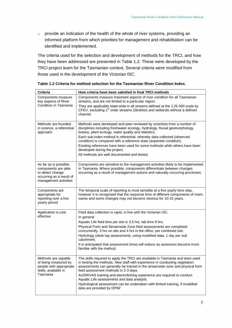
The criteria used for the selection and development of methods for the TRCI, and how they have been addressed are presented in Table 1.2. These were developed by the TRCI project team for the Tasmanian context. Several criteria were modified from those used in the development of the Victorian ISC.
Table 1.2 Criteria for method selection for the Tasmanian River Condition Index.
Criteria How criteria have been satisfied in final TRCI methods Components measure key aspects of River Condition in Tasmania
Components measure important aspects of river condition for all Tasmanian streams, and are not limited to a particular region. They are applicable state-wide in all streams defined at the 1:25 000 scale by CFEV, excluding 1st order streams (Strahler) and wetlands without a defined channel.
Methods are founded in science, a referential approach
Methods were developed and peer-reviewed by scientists from a number of disciplines including freshwater ecology, hydrology, fluvial geomorphology, botany, plant ecology, water quality and statistics. Each sub-index method is referential, whereby data collected (observed condition) is compared with a reference state (expected condition). Existing references have been used for some methods while others have been developed during the project. All methods are well documented and tested.
As far as is possible, components are able to detect change occurring as a result of management activities
Components are sensitive to the management activities likely to be implemented in Tasmania. Where possible, components differentiate between changes occurring as a result of management actions and naturally occurring processes.
Components are appropriate for reporting over a five yearly period
The temporal scale of reporting is most sensible at a five yearly time step, however it is recognised that the response time of different components of rivers varies and some changes may not become obvious for 10-15 years.
Application is cost effective
Field data collection is rapid, in line with the Victorian ISC. In general: Aquatic Life field time per site is 3.5 hrs, lab time 9 hrs; Physical Form and Streamside Zone field assessments are completed concurrently, 3 hrs on site and 4 hrs in the office, per combined site. Hydrology (desk top assessment), using modelled data, 1 day per sub catchment; It is anticipated that assessment times will reduce as assessors become more familiar with the method.
Methods are capable of being measured by people with appropriate skills, available in Tasmania
The skills required to apply the TRCI are available in Tasmania and were used in testing the methods. New staff with experience in conducting vegetation assessments can generally be trained in the streamside zone and physical form field assessment methods in 2-3 days. AUSRIVAS training and electrofishing experience are required to conduct Aquatic Life assessments and data analysis. Hydrological assessment can be undertaken with limited training, if modelled data are provided by DPIW
Tasmanian River Condition Index Reference Manual
8
Criteria How criteria have been satisfied in final TRCI methods Results are accessible to managers and easily understood
The TRCI framework and the integration of components is transparent and clearly documented The assessment process and scoring for each sub-index is well documented in clearly understood terms The majority of stream managers use the terms in the TRCI regularly. A database has been developed to store data and scores.
Methods are linked to existing programs and data collection activities
The TRCI uses a range of data layers from the CFEV database. TRCI uses this information to set context. TRCI data may be used in the future to update or validate CFEV. TRCI measures aspects of stream condition that are consistent with the scale required and the objectives of the NRMs and DPIW. Some existing programs in the State require only minor modification to incorporate TRCI into their activities. TRCI provides a mechanism for Tasmania to report on stream condition Nationally as the need arises.
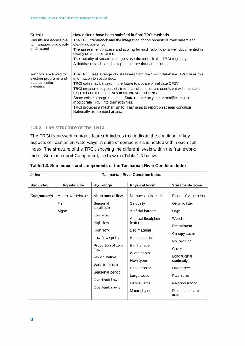
1.4.3 The structure of the TRCI The TRCI framework contains four sub-indices that indicate the condition of key aspects of Tasmanian waterways. A suite of components is nested within each sub-index. The structure of the TRCI, showing the different levels within the framework: Index, Sub-index and Component, is shown in Table 1.3 below.
Table 1.3. Sub-indices and components of the Tasmanian River Condition Index.
Index Tasmanian River Condition Index Sub index Aquatic Life Hydrology Physical Form Streamside Zone Components Macroinvertebrates
Fish
Algae
Mean annual flow
Seasonal amplitude
Low Flow
High flow
High flow
Low flow spells
Proportion of zero flow
Flow duration
Variation index
Seasonal period
Overbank flow
Overbank spells
Number of channels
Sinuosity
Artificial barriers
Artificial floodplain features
Bed material
Bank material
Bank shape
Width:depth
Flow types
Bank erosion
Large wood
Debris Jams
Macrophytes
Extent of vegetation
Organic litter
Logs
Weeds
Recruitment
Canopy cover
No. species
Cover
Longitudinal continuity
Large trees
Patch size
Neighbourhood
Distance to core area

Tasmanian River Condition Index Reference Manual
9
A fifth sub-index, ‘Water Quality’ was considered for inclusion in the TRCI. An approach based on the modelling of reach scale sediment and nutrient budgets was recommended but funding was not available to trial it, see Chapter 7. The TRCI has been designed so that should the resources arise, the Water Quality sub-index could be incorporated into the TRCI framework in the future.
1.4.4 A referential approach The TRCI has adopted a referential approach, as recommended in the FARWH (Norris et al 2006). The FARWH describes a referential approach as “an assessment of river health relative to what the river or wetland would have been like if it had not been changed by human activities” (Norris et al 2006). In the TRCI, the current condition of sites is compared with pre-European reference condition. The reference conditions used for each TRCI sub-index are detailed in Chapters 3, 4, 5 and 6.
1.5 How will the TRCI be applied? The TRCI methods are applied at the site scale and results are aggregated to the sub-catchment, catchment, regional or state scale as required. The TRCI has been designed to enable a range of reporting scales given the requirements of different users in Tasmania. The TRCI sampling strategy options (discussed in the following chapter) are robust to different reporting scales.
The TRCI has been designed to be applied to the CFEV stream network, except first order streams (based on 1:25 000 scale mapping) (CFEV database, v1.0,2005). First order streams (Strahler 1952) are not assessed as there is little confidence that they have been adequately mapped state-wide and can be unsuitable for assessment of some components of the method.
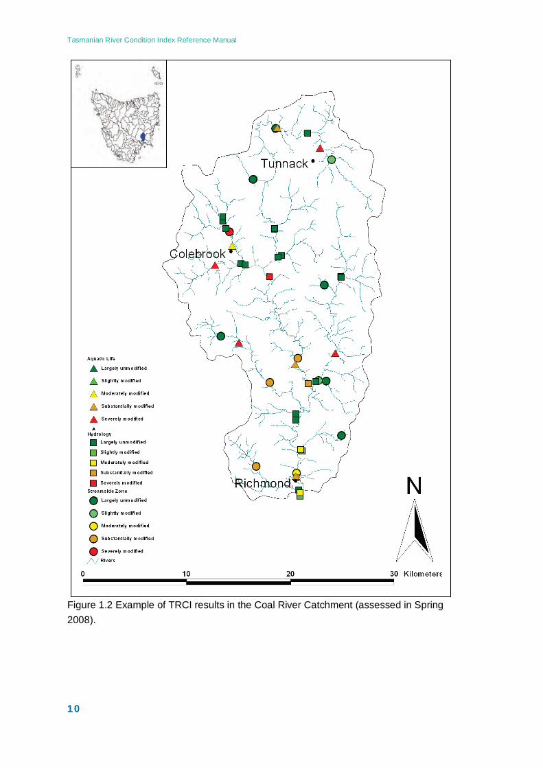
1.5.1 Example of TRCI results in a sub-catchment The components within a sub-index are measured (in the field and/or at the desktop) at sites along the stream network. Multiple sites are assessed within a given reporting unit such as a sub-catchment. Assessment site locations are not necessarily the same for each sub-index. The site selection method depends on the nature of the assessment program, the reporting unit and the sub-indices to be assessed (Chapter 2).
An example of TRCI sites and scores is presented in Figure 1.2. The results indicate that riparian vegetation and flows are generally natural or slightly modified at most sites, except in the lower reaches which are tend to be substantially or severely modified. Macro-invertebrate and fish communities are substantially or severely modified throughout the catchment
Tasmanian River Condition Index Reference Manual
10
Figure 1.2 Example of TRCI results in the Coal River Catchment (assessed in Spring 2008).
Tasmanian River Condition Index Reference Manual
11
1.6 Anticipating future improvements in condition assessment The 2009 TRCI method employs the latest techniques in stream condition assessment and data analysis, given the available budget and method objectives. Over time, further advances in this field may emerge and could be considered for inclusion in the TRCI, particularly in the area of water quality assessment.
If changes to existing TRCI methods become desirable, it is important to ensure that the results remain comparable and methods maintain the ability to show change over time. Any changes to a method must be well tested, and the implications of changing a method carefully considered. At the very least, both methods (the old and the new) should be applied concurrently at sites during the transition phase.
1.6.1 Updating reference condition Reference conditions for Aquatic Life, Physical Form and Streamside Zone are at a stage of development that reflects current data availability. It is hoped that as more data is collected, reference conditions will be further refined. Given the paucity of our knowledge of some aspects of river ecology in Tasmania, it is important that the data being collected is reviewed at regular intervals to check the validity of reference conditions and the scoring methods for each sub-index. Similarly, the models used to create the ‘natural (or reference) data set’ for the Hydrology Index will be refined in the future. The TRCI database and associated data analysis tools capture a broader range of raw data than is used in scoring, enabling site scores to be revised in the future as reference condition is updated.
1.7 References - The Development of the TRCI Anderson, J. R. (1993) State of the rivers project, Report 1. Development and validation of methodology. Queensland Department of Primary Industries. Brisbane.
Brierley, G.J. and Fryirs, K.A. (2005) Geomorphology and River Management: Applications of the RiverStyles Framework. Blackwell Science, Oxford, UK.
CFEV database, v1.0 (2005), Conservation of Freshwater Ecosystem Values Project, Water Resources Division, Department of Primary Industries and Water, Tasmania, periodic updating. Hobart.
Davies, P. E. (2008) Tasmanian River Condition Index: Testing the Draft Method, Pilot Results and Analysis- Aquatic Life Sub-Index.. A report to NRM South. Earth Tech. Wangaratta, Victoria.
Tasmanian River Condition Index Reference Manual
12
Davies, P.E. (2009) Tasmanian River Condition Index: Phase 3 Aquatic Life Sampling Results, Analysis and Recommendations for the Final TRCI Method. A report to by Freshwater Systems to NRM South. Hobart.
Dyer, F. (2008a) Tasmanian River Condition Index: Testing the Draft Method, Pilot Results and Analysis- Hydrology Sub-Index. A report to NRM South. Earth Tech. Wangaratta, Victoria.
Dyer, F. (2008b) Tasmanian River Condition Index: Physical Form Sub-Index and Recommended Way Forward. A report to NRM South. Earth Tech. Canberra.
Dyer, F.(2009) Tasmanian River Condition Index: Phase 3 Hydrology Results, Analysis and Recommendations for the Final TRCI Method. A report by Maunsell (Canberra) to NRM South. Hobart.
Department of Primary Industries Water and Environment (2006) Auditing Tasmania’s Freshwater Ecosystem Values. Conservation of Freshwater Ecosystem Values Project. Department of Primary Industries, Water and Environment, Hobart.
Department of Primary Industries and Water. (2008) Conservation of Freshwater Ecosystem Values (CFEV) Project Technical Report. Conservation of Freshwater Ecosystem Values Program, Department of Primary Industries and Water, Hobart.
Earth Tech (2007a) River Condition Index (RCI) Framework for Tasmania: Recommended Approach. A report to NRM South. Earth Tech. Wangaratta, Victoria.
Earth Tech (2007b) River Condition Index (RCI) Framework for Tasmania: Draft Method for Testing. A report to NRM South. Earth Tech. Wangaratta, Victoria.
Houshold, I., Grove, J., Spink, A. and Slijkerman, J. (2009) Tasmanian River Condition Index: Revised Physical Form Method and Application in the Leven catchment. NRM South. Hobart.
Hydro Tasmania (2009) Tasmanian River Condition Index: Data Management System v2.4 User’s Guide. Hydro Tasmania Consulting. Hobart.
Jansen, A., Robertson, A., Thompson, L. & Wilson, A., (2005) Rapid Appraisal of Riparian Condition, version 2, River Management Technical Guideline No. 4A, Land & Water Australia, Canberra.
Jansen, A. and Slijkerman, J. (2009) Tasmanian River Condition Index: Phase 3 Streamside Zone Sampling Results, Analysis and Recommendations for the Final TRCI Method. A report to NRM South. Hobart.
Krasnicki, T., Pinto, R., and Read, M. (2001) Australia wide assessment of river health: final report. Report Series WRA01/2001. DPIWE Water Management Branch, Hobart.
Tasmanian River Condition Index Reference Manual
13
Ladson, A.R., White, L.J., Doolan, J.A., Finlayson, B.L., Hart, B.T., Lake, P.S. and Tilleard, J.W. (1999) Development and testing of an Index of Stream Condition for waterway management in Australia. Freshwater Biology, 41: 453-468.
Ladson, T., and Grove, J. (2006) Assessing the Health of Tasmanian Rivers: Review of Possible Indicators. Institute for Sustainable Water Resources Monash University. Clayton, Victoria.
Michaels, K. (2006) A Manual for Assessing Vegetation Condition in Tasmania, Version 1.0. Resource Management and Conservation, Department of Primary Industries, Water and Environment, Hobart.
Murray-Darling Basin Commission (2004) Water Processes Theme Pilot Audit Technical Report – Sustainable Rivers Audit. MDBC Publication 09/04. http://www.mdbc.gov.au/__data/page/64/Web_summary_Water_Processes.pdf (accessed 5 June 2006).
Norris, R.H., Dyer, F., Hairsine, P., Kennard, M., Linke, S., Merrin, L., Read, A., Robinson, W., Ryan, C. Wilkinson, S., and Williams, D. (2007) Assessment of River and Wetland Health: A Framework for Comparative Assessment of the Ecological Condition of Australian Rivers and Wetlands National Water Commission, Canberra.
NRM South (2009a) Tasmanian River Condition Index Aquatic Life Field Manual. NRM South. Hobart.
NRM South (2009b) Tasmanian River Condition Index Hydrology User’s Manual. NRM South. Hobart.
NRM South (2009c) Tasmanian River Condition Index Physical Form Field Manual. NRM South. Hobart.
NRM South (2009d) Tasmanian River Condition Index Streamside Zone Field Manual. NRM South. Hobart.
NRM South (2009e) Tasmanian River Condition Index Guide to Data Analysis Tools. NRM South. Hobart.
Parkes, D., Newell, G. and Cheal, D. (2003) Assessing the quality of native vegetation: the ‘habitat hectares’ approach. Ecological Management and Restoration 4:S29-S37.
Robinson, W. (2009) Recommendations for the Sampling Strategy of the Tasmanian River Condition Index. A report by Riverandwetlandhealth (Marcoola, Queensland) to NRM South. Hobart.
SKM (2005) Development and Application of a Flow Stressed Ranking Procedure. A report to the Department of Sustainability and Environment, Victoria.
Tasmanian River Condition Index Reference Manual
14
Slijkerman, J., Kaye, J., Jansen A and Brown, M. (2007) Tasmanian River Condition Index: Testing the Draft Method, Pilot Results and Analysis- Streamside Zone Sub-Index. A report to NRM South. Earth Tech. Wangaratta, Victoria.
Whittington, J., Coysh, J., Davies, P., Dyer, F., Gawne, B., Lawrence, I., Liston, P., Norris, R., Robinson, W. and Thoms, M. (2001) Development of a Framework for the Sustainable Rivers Audit. Technical Report no. 8/2001. Cooperative Research Centre for Freshwater Ecology, Canberra.
Wilkinson (2007) The Feasibility of Using SedNet to Assess Water Quality in the Tasmanian River Condition Index. A report to NRM South. Earth Tech. Townsville, Queensland.
Tasmanian River Condition Index Reference Manual
15
Appendix to Chapter 1: Further detail on the TRCI project
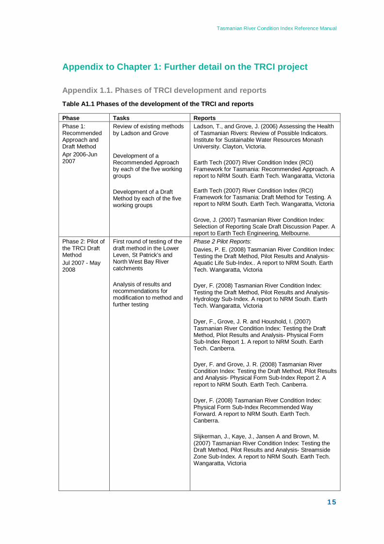
Appendix 1.1. Phases of TRCI development and reports Table A1.1 Phases of the development of the TRCI and reports
Phase Tasks Reports Phase 1: Recommended Approach and Draft Method Apr 2006-Jun 2007
Review of existing methods by Ladson and Grove Development of a Recommended Approach by each of the five working groups Development of a Draft Method by each of the five working groups
Ladson, T., and Grove, J. (2006) Assessing the Health of Tasmanian Rivers: Review of Possible Indicators. Institute for Sustainable Water Resources Monash University. Clayton, Victoria. Earth Tech (2007) River Condition Index (RCI) Framework for Tasmania: Recommended Approach. A report to NRM South. Earth Tech. Wangaratta, Victoria Earth Tech (2007) River Condition Index (RCI) Framework for Tasmania: Draft Method for Testing. A report to NRM South. Earth Tech. Wangaratta, Victoria Grove, J. (2007) Tasmanian River Condition Index: Selection of Reporting Scale Draft Discussion Paper. A report to Earth Tech Engineering, Melbourne.
Phase 2: Pilot of the TRCI Draft Method Jul 2007 - May 2008
First round of testing of the draft method in the Lower Leven, St Patrick’s and North West Bay River catchments Analysis of results and recommendations for modification to method and further testing
Phase 2 Pilot Reports: Davies, P. E. (2008) Tasmanian River Condition Index: Testing the Draft Method, Pilot Results and Analysis- Aquatic Life Sub-Index.. A report to NRM South. Earth Tech. Wangaratta, Victoria Dyer, F. (2008) Tasmanian River Condition Index: Testing the Draft Method, Pilot Results and Analysis- Hydrology Sub-Index. A report to NRM South. Earth Tech. Wangaratta, Victoria Dyer, F., Grove, J. R. and Houshold, I. (2007) Tasmanian River Condition Index: Testing the Draft Method, Pilot Results and Analysis- Physical Form Sub-Index Report 1. A report to NRM South. Earth Tech. Canberra. Dyer, F. and Grove, J. R. (2008) Tasmanian River Condition Index: Testing the Draft Method, Pilot Results and Analysis- Physical Form Sub-Index Report 2. A report to NRM South. Earth Tech. Canberra. Dyer, F. (2008) Tasmanian River Condition Index: Physical Form Sub-Index Recommended Way Forward. A report to NRM South. Earth Tech. Canberra. Slijkerman, J., Kaye, J., Jansen A and Brown, M. (2007) Tasmanian River Condition Index: Testing the Draft Method, Pilot Results and Analysis- Streamside Zone Sub-Index. A report to NRM South. Earth Tech. Wangaratta, Victoria
Tasmanian River Condition Index Reference Manual
16
Phase Tasks Reports Wilkinson (2007) The Feasibility of Using SedNet to Assess Water Quality in the Tasmanian River Condition Index. A report to NRM South. Earth Tech. Townsville, Queensland.
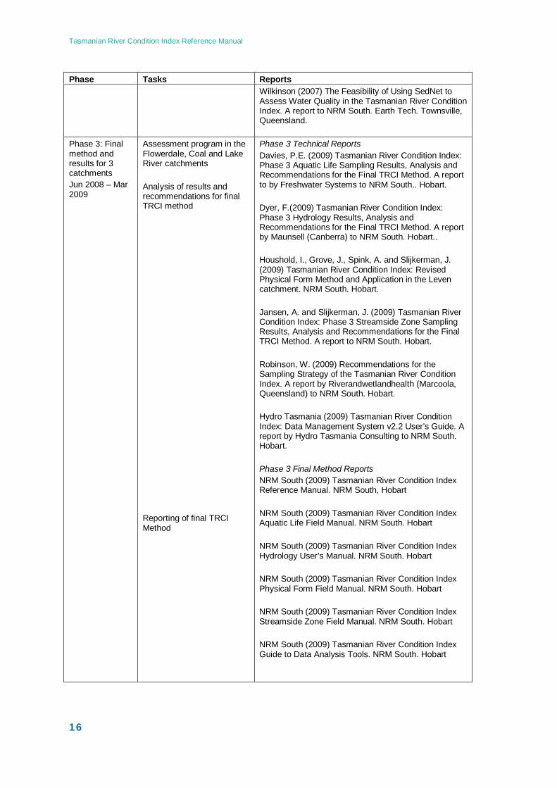
Phase 3: Final method and results for 3 catchments Jun 2008 – Mar 2009
Assessment program in the Flowerdale, Coal and Lake River catchments Analysis of results and recommendations for final TRCI method Reporting of final TRCI Method
Phase 3 Technical Reports Davies, P.E. (2009) Tasmanian River Condition Index: Phase 3 Aquatic Life Sampling Results, Analysis and Recommendations for the Final TRCI Method. A report to by Freshwater Systems to NRM South.. Hobart. Dyer, F.(2009) Tasmanian River Condition Index: Phase 3 Hydrology Results, Analysis and Recommendations for the Final TRCI Method. A report by Maunsell (Canberra) to NRM South. Hobart.. Houshold, I., Grove, J., Spink, A. and Slijkerman, J. (2009) Tasmanian River Condition Index: Revised Physical Form Method and Application in the Leven catchment. NRM South. Hobart. Jansen, A. and Slijkerman, J. (2009) Tasmanian River Condition Index: Phase 3 Streamside Zone Sampling Results, Analysis and Recommendations for the Final TRCI Method. A report to NRM South. Hobart. Robinson, W. (2009) Recommendations for the Sampling Strategy of the Tasmanian River Condition Index. A report by Riverandwetlandhealth (Marcoola, Queensland) to NRM South. Hobart. Hydro Tasmania (2009) Tasmanian River Condition Index: Data Management System v2.2 User’s Guide. A report by Hydro Tasmania Consulting to NRM South. Hobart. Phase 3 Final Method Reports NRM South (2009) Tasmanian River Condition Index Reference Manual. NRM South, Hobart NRM South (2009) Tasmanian River Condition Index Aquatic Life Field Manual. NRM South. Hobart NRM South (2009) Tasmanian River Condition Index Hydrology User’s Manual. NRM South. Hobart NRM South (2009) Tasmanian River Condition Index Physical Form Field Manual. NRM South. Hobart NRM South (2009) Tasmanian River Condition Index Streamside Zone Field Manual. NRM South. Hobart NRM South (2009) Tasmanian River Condition Index Guide to Data Analysis Tools. NRM South. Hobart

Tasmanian River Condition Index Reference Manual
17
2 Applying the TRCI The procedure for completing a TRCI assessment program is as follows:
1. Define the objectives of the assessment program;
2. Determine the spatial scale of assessment (e.g. particular sites, regions, catchments, state-wide), and hence the reporting unit;
3. Determine which sub-indices are to be assessed as part of the program;
4. Determine the required level of confidence for the project, and hence the number of sites to be sampled;
5. Determine the appropriate sampling strategy and select sites;
6. Complete field and desktop measurements of components and score each sub-index;
7. Aggregate site scores to give sub-index scores for the reporting unit/s.
2.1 Defining objectives The TRCI can be used for various types of assessment including:
o Assessments (either one-off or repeated) of the condition of streams within specified areas (e.g. catchments, NRM regions, state-wide);
o Long-term monitoring of the effects of river works or other impacts on the condition of the river;
o Assessments of the condition of rivers in relation to management units or practices of interest (e.g. logged vs unlogged catchments, altered vs unaltered flow regimes, urban vs rural catchments, etc.).
The type of assessment will determine the scale of the assessment program, the reporting units, the required level of confidence, and the appropriate sampling strategy. General advice on each of these points for each type of assessment will be given here, but for any particular project, detailed advice should be sought from an experienced statistician prior to commencing the assessments.
2.2 Spatial scale and reporting units TRCI assessments are site-based and may be aggregated to give scores for areas of interest. The location of assessment sites for different sub-indices within an area of interest may differ. The TRCI is flexible in its reporting scale in order to accommodate the requirements of different users in Tasmania. During the development of the TRCI, the primary reporting scale agreed by DPIW and the NRMs was the TRCI sub-
Tasmanian River Condition Index Reference Manual
18
catchment (100-500km2: based on amalgamations of smaller CFEV sub-catchments). However, the TRCI sub-index scores can be aggregated at other scales such as the sub-catchment, catchment, regional or state scale. If wishing to report at a scale other than the TRCI sub catchment, then the sampling strategy (see below) must by applied at that scale. If wishing to report across various scales (e.g. a catchment of interest as well as an entire NRM jurisdiction) then the sampling strategy must be applied at the smallest scale of interest (e.g. the catchment of interest) and results aggregated to the larger scale.
2.2.1 Stream network The TRCI has been designed to be applied to the CFEV (2005) stream network, with the exception of first order (Strahler 1952) streams (based on 1:25 000 scale mapping). First order streams (Strahler 1952) are not assessed as there is little confidence that they have been adequately mapped state-wide.
There are also a variety of reasons specific to each sub-index for excluding first order streams (for example, in relation to the aquatic life sub-index, these streams are often dry at the time of sampling, they often lack fish, they have highly variable macroinvertebrate and algal communities and are difficult to characterise, and often lack significant patches of riffle habitat essential for sampling macroinvertebrates). Similarly, wetlands without a defined channel and estuaries are not assessed. These systems are beyond the scope of the TRCI and TRCI field methods are inappropriate.
2.3 Which sub-indices to assess? The sub-indices assessed depend on the objectives of the assessment program and the resources available. In general, for an overall assessment of river condition, all sub-indices should be used, since each provides information on different aspects of river condition, with different sensitivities and rates of response to various drivers (e.g. direct impacts, natural events). However, if a targeted monitoring program is being developed to examine the effects of river works or effects of management practices, the sub-indices may be selected based on the types of river works or impacts. For example, riparian planting will have most immediate impact on the Streamside Zone sub-index and smaller and longer-term impacts on the other sub-indices (depending on the scale of the project). On the other hand, a comparison of river condition adjacent to organic farming practices vs conventional farming practices, may be most usefully made using the Aquatic Life sub-index, since little change would be expected in the Hydrology and Physical Form sub-indices.

Tasmanian River Condition Index Reference Manual
19
2.4 Number of sites and confidence required Levels of precision and confidence required for specific projects will vary according to the objectives of the project, and need to be considered before deciding on numbers of sites required. For example the levels of precision and the confidence required for a program to detect changes in river condition as a result of river works may be higher than that required for a general assessment of river condition across the State. In general the project team recommend that TRCI assessment results should aim to be precise to +/-10% with 80% confidence (or 0.1 half width of 80% confidence interval in Figure 2.1 and Figure 2.2 below).
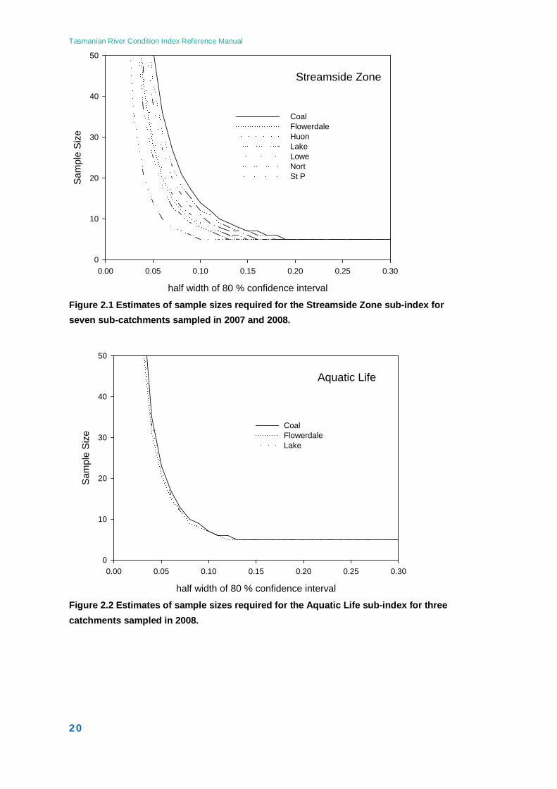
The number of sites required to be assessed per sub-index within a given reporting unit to return a specified level of confidence, will depend on both the sub-catchment and the sub-index. Data from the pilot studies conducted in 2007 and 2008 were used to estimate sample sizes required to give scores to within 10% of their true value with 80% confidence. Data were available for seven sub-catchments for the streamside zone sub-index (Figure 2.1), and for three sub-catchments for the aquatic life sub-index (Figure 2.2).
Tasmanian River Condition Index Reference Manual
20
Figure 2.1 Estimates of sample sizes required for the Streamside Zone sub-index for seven sub-catchments sampled in 2007 and 2008.
Figure 2.2 Estimates of sample sizes required for the Aquatic Life sub-index for three catchments sampled in 2008.
Streamside Zone
half width of 80 % confidence interval
0.00 0.05 0.10 0.15 0.20 0.25 0.30
Sam
ple
Siz
e
0
10
20
30
40
50
Coal Flowerdale HuonLake Lowe Nort St P
Aquatic Life
half width of 80 % confidence interval
0.00 0.05 0.10 0.15 0.20 0.25 0.30
Sam
ple
Siz
e
0
10
20
30
40
50
Coal Flowerdale Lake
Tasmanian River Condition Index Reference Manual
21
Figures 2.1 and 2.2 suggest that 15 sites per sub-catchment are required for the streamside zone sub-index, and 8 sites per sub-catchment for the aquatic life sub-index. No data are yet available for the physical form sub-index. The hydrology sub-index uses modelled data from available nodes within each sub-catchment. It is recommended that data from all standard nodes be used.
It must be noted that the recommended number of sites per sub-catchment are estimates only and as more data are collected in different sub-catchments, further statistical analysis should be conducted. Over-sampling will minimise the risk of having low confidence in results. Alternatively a reconnaissance survey could be conducted to gauge variation.
It should also be noted that these estimates are based on aggregating site scores at the TRCI sub-catchment level for reporting at this scale. It is possible that reporting at a different scale may result in required numbers of sites being somewhat different, although it appears that the sample size is not overly dependent on the area to be sampled. This has been shown to be the case for most themes in the Murray Darling Basin Authority’s SRA project (Wayne Robinson pers. comm., 2009).
Prior to each assessment program the objectives of the project must be carefully defined. This allows a benefit to cost analysis of the consequences of certain tolerances, the selection of an appropriate level of confidence for the project and an appropriate sampling strategy. If +/-10% at the 80% confidence interval is not appropriate, more sites may need to be assessed.
2.5 Site selection This section describes the different site selection methods recommended for the TRCI. Examples are provided in Appendix 2. The incorporation of additional sites into a sampling program and issues of missing data are also addressed.
Sites should be selected randomly along the stream network (excluding Strahler first order streams, wetlands and estuaries) using basic random sampling (BR), probabilistic random sampling (PRS) or stratified sampling (SS), depending on the objectives of the assessment program. It is important to note that, as different numbers of sites may be required for different sub-indices, site selection may need to be done separately for each sub-index. For the Streamside Zone sub-index, the bank (left bank/right bank) to be assessed should also be assigned randomly at the desktop.
2.5.1 Basic random (BR) sampling Basic random (BR) sampling can be used when every part of the catchment is to be sampled and given equal weight in the assessment. Effectively, areas of the catchment with more stream length will have more sites allocated in them. If there is a strata that occurs unevenly in the catchment, such as sandstone versus volcanic
Tasmanian River Condition Index Reference Manual
22
geology, 80% and 20% of the catchment respectively, then they will be represented approximately in these proportions in the analysis. If the strata are related to the assessment variable they may give undesirable results. Imagine a catchment that has 75% of its stream length as second order streams and these are in very good hydrological condition but the remaining 25% of streams are highly regulated. 75% of sites will fall into second order streams and the overall catchment condition assessment for hydrology will be high. In other words, it is the length of stream that weights the assessment. If the volume of water flowing was more important than length of stream then the use of strata by stream order or weighting by flow rather than length could be used.
The BR method is intuitively suitable for the Streamside Zone sub-index or an assessment of in-channel vegetation condition because the condition of the vegetation along the entire stream network is given equal weight in the analysis. If the measure is potentially affected by the flow or stream size (say there is an accumulation of effects like WQ or sedimentation) then another method may be desired.
2.5.2 Probabilistic random sampling (PRS) Probabilistic Random Sampling (PRS) can be used when every site does not need to have an equally likely chance of being selected. The BR method may result in some regions having considerably more sites than others and this could be undesirable if the assessment is influenced by the region. Say an area with lots of second order streams is also heavily disturbed by logging. The BR method will result in a high incidence of sites in parts of the catchment that are logged. Using PRS will ensure that these sites scores are still represented in the analysis by weighting, but will also allow sites in other regions more chance of being sampled.
PRS should be used when there is a strong desire to spread sites out across the catchment, but not to under-represent regions with many smaller stream lengths and over-represent sites from regions with very few sites to choose from.
The PRS type approach can also be set up with or without constraints to assure the spatial coverage. A method for this is also described in Appendix 2, called probabilistic random reach sampling (PRR). It is suited to sub-indicies where one sample can be inferred to be representative of a determined stream length. This would be typical of a hydrology or modelled sub-index, or some of the landscape component of the Streamside Zone sub-index. Some programs infer that a single site score for say fish health can be applied to the entire reach and then use the same weighting method as described here. In Appendix 2 an example where one point is sampled at random within the determined stream length, such as used in the fish and macroinvertebrate themes for the SRA and for the FARWH, is presented. An example using modelled data, where one score is modelled for an entire length of stream, typical of a hydrology sub-index is also shown in Appendix 2.
Tasmanian River Condition Index Reference Manual
23
2.5.3 Stratified sampling (SS) Stratified Sampling (SS) should only ever be used if it is desirable to report on strata within the larger spatial scale (say catchment). For instance, if it is desirable to report on condition of the two types of geology separately as well as the overall catchment condition.
2.5.4 Additional sites If resources become available to assess additional sites, they must be selected randomly to be representative. If sampling has not commenced, the entire spatial framework can be redesigned and the new sites added. If sampling has already commenced, there are two options to incorporate these additional sites;
o the new sites can be selected at random within the randomly selected spatial units o if a region within the catchment (say a strata or management unit) is of specific
interest, then sites can be randomly allocated to that region
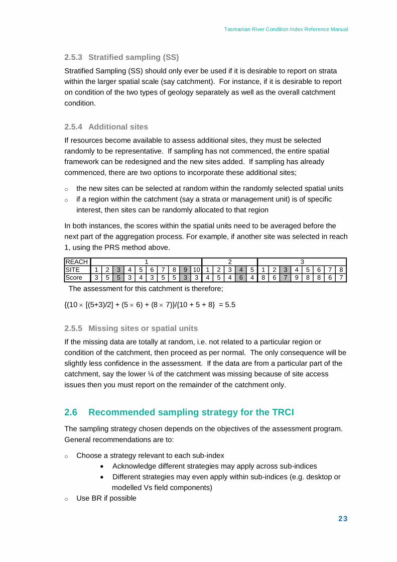
In both instances, the scores within the spatial units need to be averaged before the next part of the aggregation process. For example, if another site was selected in reach 1, using the PRS method above.
The assessment for this catchment is therefore;
{(10 × [(5+3)/2] + (5 × 6) + (8 × 7)}/{10 + 5 + 8} = 5.5
2.5.5 Missing sites or spatial units If the missing data are totally at random, i.e. not related to a particular region or condition of the catchment, then proceed as per normal. The only consequence will be slightly less confidence in the assessment. If the data are from a particular part of the catchment, say the lower ¼ of the catchment was missing because of site access issues then you must report on the remainder of the catchment only.
2.6 Recommended sampling strategy for the TRCI The sampling strategy chosen depends on the objectives of the assessment program. General recommendations are to:
o Choose a strategy relevant to each sub-index • Acknowledge different strategies may apply across sub-indices • Different strategies may even apply within sub-indices (e.g. desktop or
modelled Vs field components) o Use BR if possible
REACH 1 2 3SITE 1 2 3 4 5 6 7 8 9 10 1 2 3 4 5 1 2 3 4 5 6 7 8Score 3 5 5 3 4 3 5 5 3 3 4 5 4 6 4 8 6 7 9 8 8 6 7
Tasmanian River Condition Index Reference Manual
24
o Use PRS or PRR otherwise o Avoid SS if at all possible
2.7 Field and desktop measurements and scoring Once the sampling strategy and sub-indices to be assessed have been decided, the field and desktop work can be completed. Detailed instructions on the methods for each sub-index can be found in the following chapters. It should be noted that the ideal time for sampling each sub-index varies, as detailed in each chapter.
Data analysis tools are listed below. The TRCI database is the primary data storage tool. The database and the Tasmanian River Condition Index Guide to Data Analysis Tools (NRM South 2009e) can be obtained from NRM South. Details of how to obtain sub-index specific tools are listed in the sub-index chapters of this report.
o TRCI Database o TRCI Aquatic Life data entry spreadsheet for fish o TRCI Aquatic Life data analysis and integration spreadsheet o Online AUSRIVAS models o TRCI Hydrology programs o DPIW Hydrological models o TRCI Physical Form geomorphic benchmarks for data analysis o TRCI Physical Form Arc GIS ‘potential for river type change’ shapefile o TRCI Streamside Zone desktop landscape component Arc GIS shapefile and
calculation tool o TRCI Sub-catchment Arc GIS shapefile
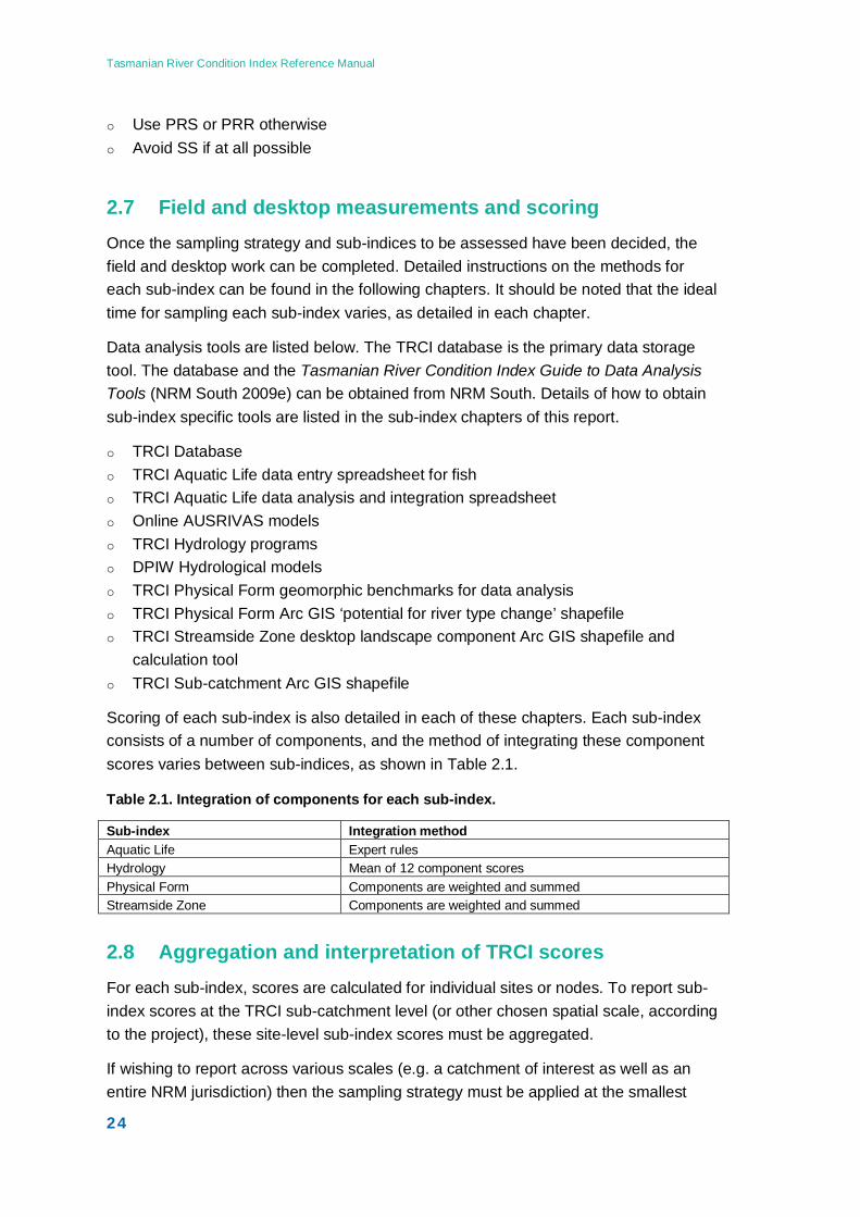
Scoring of each sub-index is also detailed in each of these chapters. Each sub-index consists of a number of components, and the method of integrating these component scores varies between sub-indices, as shown in Table 2.1.
Table 2.1. Integration of components for each sub-index.
Sub-index Integration method Aquatic Life Expert rules Hydrology Mean of 12 component scores Physical Form Components are weighted and summed Streamside Zone Components are weighted and summed
2.8 Aggregation and interpretation of TRCI scores For each sub-index, scores are calculated for individual sites or nodes. To report sub-index scores at the TRCI sub-catchment level (or other chosen spatial scale, according to the project), these site-level sub-index scores must be aggregated.
If wishing to report across various scales (e.g. a catchment of interest as well as an entire NRM jurisdiction) then the sampling strategy must be applied at the smallest
Tasmanian River Condition Index Reference Manual
25
scale of interest (e.g. the catchment of interest) and results aggregated to the larger scale
It is recommended that medians of the site scores are used for aggregation of the Aquatic Life, Physical Form and Streamside Zone sub-indices (weighted if necessary, depending on the sampling strategy). The Hydrology sub-index uses a weighted median. The method for calculating the weighted median is described in Chapter 4.
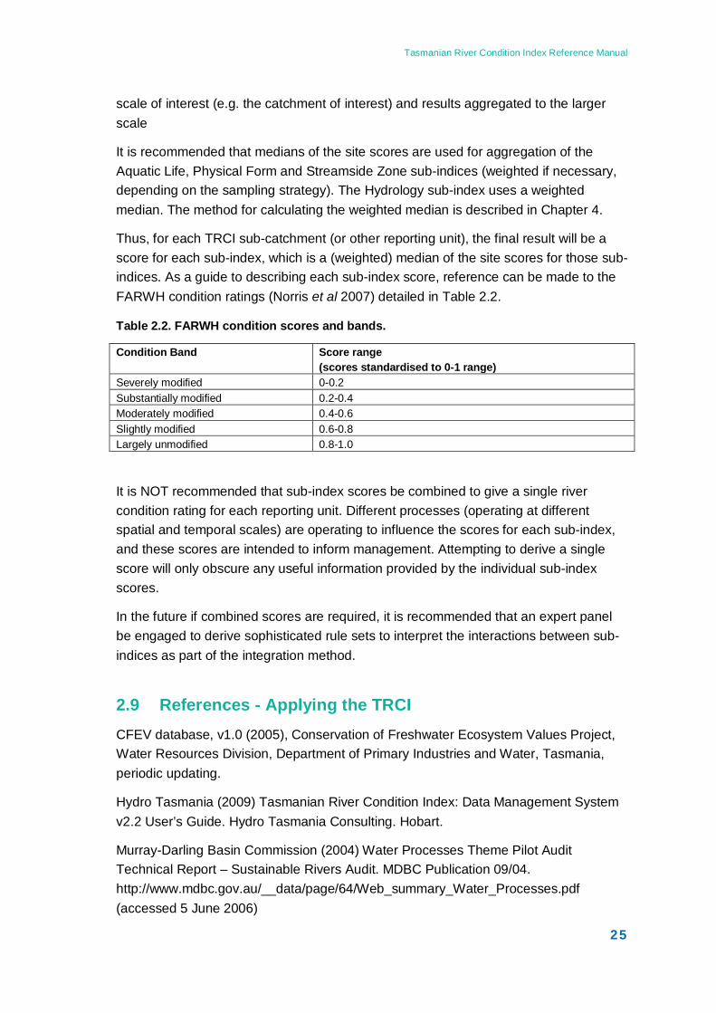
Thus, for each TRCI sub-catchment (or other reporting unit), the final result will be a score for each sub-index, which is a (weighted) median of the site scores for those sub-indices. As a guide to describing each sub-index score, reference can be made to the FARWH condition ratings (Norris et al 2007) detailed in Table 2.2.
Table 2.2. FARWH condition scores and bands.
Condition Band Score range (scores standardised to 0-1 range)
Severely modified 0-0.2 Substantially modified 0.2-0.4 Moderately modified 0.4-0.6 Slightly modified 0.6-0.8 Largely unmodified 0.8-1.0
It is NOT recommended that sub-index scores be combined to give a single river condition rating for each reporting unit. Different processes (operating at different spatial and temporal scales) are operating to influence the scores for each sub-index, and these scores are intended to inform management. Attempting to derive a single score will only obscure any useful information provided by the individual sub-index scores.
In the future if combined scores are required, it is recommended that an expert panel be engaged to derive sophisticated rule sets to interpret the interactions between sub-indices as part of the integration method.
2.9 References - Applying the TRCI CFEV database, v1.0 (2005), Conservation of Freshwater Ecosystem Values Project, Water Resources Division, Department of Primary Industries and Water, Tasmania, periodic updating.
Hydro Tasmania (2009) Tasmanian River Condition Index: Data Management System v2.2 User’s Guide. Hydro Tasmania Consulting. Hobart.
Murray-Darling Basin Commission (2004) Water Processes Theme Pilot Audit Technical Report – Sustainable Rivers Audit. MDBC Publication 09/04. http://www.mdbc.gov.au/__data/page/64/Web_summary_Water_Processes.pdf (accessed 5 June 2006)
Tasmanian River Condition Index Reference Manual
26
Norris, R.H., Dyer, F., Hairsine, P., Kennard, M., Linke, S., Merrin, L., Read, A., Robinson, W., Ryan, C. Wilkinson, S., and Williams, D. (2007) Assessment of River and Wetland Health: A Framework for Comparative Assessment of the Ecological Condition of Australian Rivers and Wetlands National Water Commission, Canberra.
NRM South (2009a) Tasmanian River Condition Index Aquatic Life Field Manual. NRM South. Hobart.
NRM South (2009b) Tasmanian River Condition Index Hydrology User’s Manual. NRM South. Hobart.
NRM South (2009c) Tasmanian River Condition Index Physical Form Field Manual. NRM South. Hobart.
NRM South (2009d) Tasmanian River Condition Index Streamside Zone Field Manual. NRM South. Hobart.
NRM South (2009e) Tasmanian River Condition Index Guide to Data Analysis Tools. NRM South. Hobart.
Robinson, W. (2009) Recommendations for the Sampling Strategy of the Tasmanian River Condition Index. A report by Riverandwetlandhealth (Marcoola, Queensland) to NRM South. Hobart.
Strahler, A., N. (1952) Hypsometric (area altitude) analysis of erosional topography. Bulletin of the Geological Society of America, 63:923-38.

Tasmanian River Condition Index Reference Manual
27

Tasmanian River Condition Index Reference Manual
28
Appendix to Chapter 2: Further detail on TRCI sampling Appendix 2.1 Examples of sampling methods
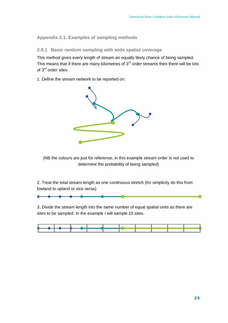
Tasmanian River Condition Index Reference Manual
29
Appendix 2.1. Examples of sampling methods
2.9.1 Basic random sampling with wide spatial coverage This method gives every length of stream an equally likely chance of being sampled. This means that if there are many kilometres of 3rd order streams then there will be lots of 3rd order sites.
1. Define the stream network to be reported on:
(NB the colours are just for reference, in this example stream order is not used to determine the probability of being sampled)
2. Treat the total stream length as one continuous stretch (for simplicity do this from lowland to upland or vice versa)
3. Divide the stream length into the same number of equal spatial units as there are sites to be sampled. In the example I will sample 10 sites.
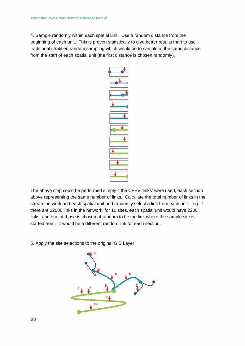
Tasmanian River Condition Index Reference Manual
30
4. Sample randomly within each spatial unit. Use a random distance from the beginning of each unit. This is proven statistically to give better results than to use traditional stratified random sampling which would be to sample at the same distance from the start of each spatial unit (the first distance is chosen randomly).
The above step could be performed simply if the CFEV ‘links’ were used, each section above representing the same number of links. Calculate the total number of links in the stream network and each spatial unit and randomly select a link from each unit. e.g. If there are 22000 links in the network, for 10 sites, each spatial unit would have 2200 links, and one of those is chosen at random to be the link where the sample site is started from. It would be a different random link for each section.
5. Apply the site selections to the original GIS Layer
1
2
34 5
67
9
8
10
1
2
34 5
67
9
8
10
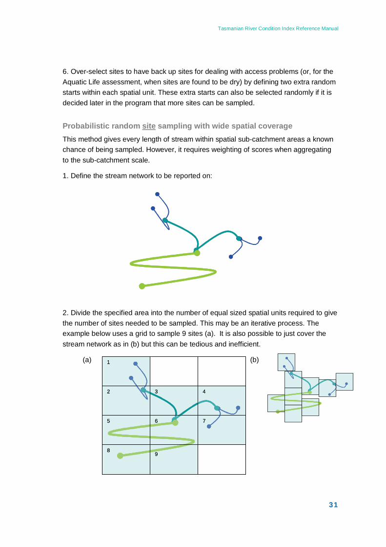
Tasmanian River Condition Index Reference Manual
31
6. Over-select sites to have back up sites for dealing with access problems (or, for the Aquatic Life assessment, when sites are found to be dry) by defining two extra random starts within each spatial unit. These extra starts can also be selected randomly if it is decided later in the program that more sites can be sampled.
Probabilistic random siteThis method gives every length of stream within spatial sub-catchment areas a known chance of being sampled. However, it requires weighting of scores when aggregating to the sub-catchment scale.
sampling with wide spatial coverage
1. Define the stream network to be reported on:
2. Divide the specified area into the number of equal sized spatial units required to give the number of sites needed to be sampled. This may be an iterative process. The example below uses a grid to sample 9 sites (a). It is also possible to just cover the stream network as in (b) but this can be tedious and inefficient.
(a)
(b)
1
3 4
5 6 7
89
2
1
3 4
5 6 7
89
2
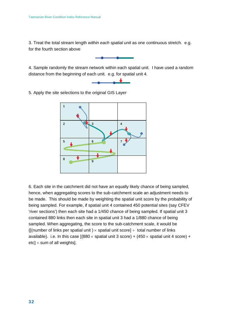
Tasmanian River Condition Index Reference Manual
32
3. Treat the total stream length within each spatial unit as one continuous stretch. e.g. for the fourth section above
4. Sample randomly the stream network within each spatial unit. I have used a random distance from the beginning of each unit. e.g. for spatial unit 4.
5. Apply the site selections to the original GIS Layer
6. Each site in the catchment did not have an equally likely chance of being sampled, hence, when aggregating scores to the sub-catchment scale an adjustment needs to be made. This should be made by weighting the spatial unit score by the probability of being sampled. For example, if spatial unit 4 contained 450 potential sites (say CFEV ‘river sections’) then each site had a 1/450 chance of being sampled. If spatial unit 3 contained 880 links then each site in spatial unit 3 had a 1/880 chance of being sampled. When aggregating, the score to the sub-catchment scale, it would be {[(number of links per spatial unit ) × spatial unit score] ÷ total number of links available}. i.e. In this case [(880 × spatial unit 3 score) + (450 × spatial unit 4 score) + etc] ÷ sum of all weights].
1
3 4
5 6 7
89
2
1
3 4
5 6 7
89
2

Tasmanian River Condition Index Reference Manual
33
An example of this is given below. In this example catchment there are only three reaches. One with 10 potential sites, one with 5 sites and one with 8 sites. The randomly sampled site in each reach is shaded.
The assessment for this catchment is therefore;
{(10 × 5) + (5 × 6) + (8 × 7)}/{10 + 5 + 8} = 5.9
REACH 1 2 3SITE 1 2 3 4 5 6 7 8 9 10 1 2 3 4 5 1 2 3 4 5 6 7 8Score 3 5 5 3 4 3 5 5 3 3 4 5 4 6 4 8 6 7 9 8 8 6 7
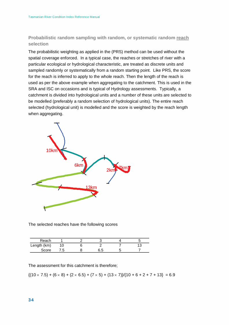
Tasmanian River Condition Index Reference Manual
34
Probabilistic random sampling with random, or systematic random reach
The probabilistic weighting as applied in the (PRS) method can be used without the spatial coverage enforced. In a typical case, the reaches or stretches of river with a particular ecological or hydrological characteristic, are treated as discrete units and sampled randomly or systematically from a random starting point. Like PRS, the score for the reach is inferred to apply to the whole reach. Then the length of the reach is used as per the above example when aggregating to the catchment. This is used in the SRA and ISC on occasions and is typical of Hydrology assessments. Typically, a catchment is divided into hydrological units and a number of these units are selected to be modelled (preferably a random selection of hydrological units). The entire reach selected (hydrological unit) is modelled and the score is weighted by the reach length when aggregating.
selection
The selected reaches have the following scores
The assessment for this catchment is therefore;
{(10 × 7.5) + (6 × 8) + (2 × 6.5) + (7 × 5) + (13 × 7)}/{10 + 6 + 2 + 7 + 13} = 6.9
10km
6km2km 7km
13km
10km
6km2km 7km
13km
Reach 1 2 3 4 5Length (km) 10 6 2 7 13
Score 7.5 8 6.5 5 7
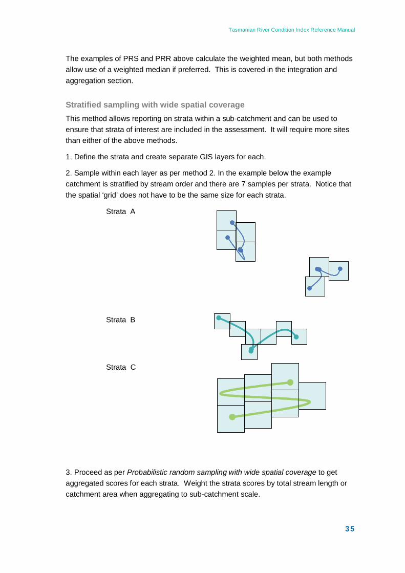
Tasmanian River Condition Index Reference Manual
35
The examples of PRS and PRR above calculate the weighted mean, but both methods allow use of a weighted median if preferred. This is covered in the integration and aggregation section.
Stratified sampling with wide spatial coverage This method allows reporting on strata within a sub-catchment and can be used to ensure that strata of interest are included in the assessment. It will require more sites than either of the above methods.
1. Define the strata and create separate GIS layers for each.
2. Sample within each layer as per method 2. In the example below the example catchment is stratified by stream order and there are 7 samples per strata. Notice that the spatial ‘grid’ does not have to be the same size for each strata.
Strata A
Strata B
Strata C
3. Proceed as per Probabilistic random sampling with wide spatial coverage to get aggregated scores for each strata. Weight the strata scores by total stream length or catchment area when aggregating to sub-catchment scale.

Tasmanian River Condition Index Reference Manual
36
If wishing to report at a scale other than the TRCI sub catchment, then apply the selection strategy at that scale. If wishing to report across various scales (e.g. a catchment of interest as well as an entire NRM jurisdiction) then the sampling strategy must be applied at the smallest scale of interest (e.g. the catchment of interest) and results aggregated to the larger scale.
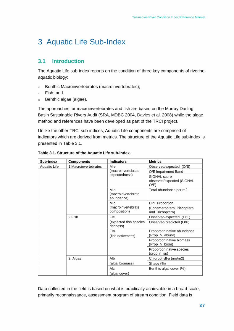
Tasmanian River Condition Index Reference Manual
37
3 Aquatic Life Sub-Index
3.1 Introduction The Aquatic Life sub-index reports on the condition of three key components of riverine aquatic biology:
o Benthic Macroinvertebrates (macroinvertebrates); o Fish; and o Benthic algae (algae).
The approaches for macroinvertebrates and fish are based on the Murray Darling Basin Sustainable Rivers Audit (SRA, MDBC 2004, Davies et al. 2008) while the algae method and references have been developed as part of the TRCI project.
Unlike the other TRCI sub-indices, Aquatic Life components are comprised of indicators which are derived from metrics. The structure of the Aquatic Life sub-index is presented in Table 3.1.
Table 3.1. Structure of the Aquatic Life sub-index.
Sub-index Components Indicators Metrics Aquatic Life 1.Macroinvertebrates MIe
(macroinvertebrate expectedness)
Observed/expected (O/E) O/E Impairment Band
SIGNAL score observed/expected (SIGNAL O/E)
MIa (macroinvertebrate abundance)
Total abundance per m2
MIc (macroinvertebrate composition)
EPT Proportion (Ephemeroptera, Plecoptera and Trichoptera)
2.Fish FIe (expected fish species richness)
Observed/expected (O/E) Observed/predicted (O/P)
FIn (fish nativeness)
Proportion native abundance (Prop_N_abund) Proportion native biomass (Prop_N_biom) Proportion native species (prop_n_sp)
3. Algae Alb (algal biomass)
Chlorophyll-a (mg/m2) Shade (%)
Alc (algal cover)
Benthic algal cover (%)
Data collected in the field is based on what is practically achievable in a broad-scale, primarily reconnaissance, assessment program of stream condition. Field data is
Tasmanian River Condition Index Reference Manual
38
reported as metrics which are benchmarked against reference condition. Reference condition is equated to the pre-European or ‘natural’ state. Reference condition is derived from a variety of data sources, using both data sets from least impaired sites (for macroinvertebrate and algal metrics), and data derived from expert-derived mapping rules (the native fish data in CFEV).
An important resource for the Aquatic Life sub-index of the TRCI is the Conservation of Freshwater Ecosystem Values (CFEV) framework GIS database (DPIW 2008). This is used to provide data on reference condition for native fish, as well as catchment and other spatial data on Tasmanian river systems.
3.2 Background, component selection and rationale The TRCI Recommended Approach (Earth Tech 2007) suggested that an assessment of the condition of aquatic life in Tasmanian rivers should incorporate measures of the state of key biological elements as well as some measures of ecosystem processes (Earth Tech, 2007).
In addition to the specified TRCI selection criteria used during the development of the methods (Chapter 1), the following criteria were used to guide the selection of components for the Aquatic Life sub-index:
o the presence of cost-effective sampling and analytical methods; o the ability to describe and quantify natural reference condition as a benchmark for
assessment and reporting; o the ability to interpret results from an assessment; o whether the indicator is a core component or aspect of ecosystem state and
function; o whether the indicator is responsive to human-induced environmental change; and o whether measures of the indicator take into account natural spatial and temporal
variability and/or context.
Following an assessment of current practice in Tasmania and of a series of potential components against these criteria, the final components to be included were:
o assessments of benthic macroinvertebrates; o fish; and o benthic algae (chlorophyll-a).
These key aspects of instream biological ‘structure’ were considered to provide valuable information on instream ecosystem condition. All of these were assessable by either existing or readily adaptable methods. They are described further in Section 3.3.
Components of interest but for which sampling, analytical methods or supporting reference data were not readily available, or were difficult and/or expensive, included
Tasmanian River Condition Index Reference Manual
39
other vertebrates (such as platypus, water rats, birds, frogs), micro-invertebrates such as rotifers, fungi, bacteria, and crayfish.
Key instream ecosystem processes identified for potential assessment included nutrient transformation and dynamics, rates of primary production and respiration and trophic pathways for organic carbon and nitrogen.
Macrophytes, benthic diatoms and ecosystem processes have been flagged for potential inclusion in the TRCI in the future. At present they have not been included as they lack formal analysis, interpretation frameworks and fully developed reference conditions. These components were deemed to be more in the realm of ‘research’ rather than ‘routine’ or current practice. Investigating these components further was beyond the resources available to the TRCI project.
3.3 Aquatic Life reference conditions The TRCI Aquatic Life methods use established reference condition for macroinvertebrate O/E and SIGNAL O/E metrics. In addition, reference condition for the nativeness fish metrics, based on ratios of native to exotic fish numbers, taxa and biomass, were defined by the absence of alien species under natural conditions, rating the highest score (100). Sites with 100% exotic fish were rated 0.
However, reference conditions for macroinvertebrate EPT ratio and abundance metrics, fish community composition, fish O/E and O/P metrics, algal chlorophyll-a and algal cover were developed specifically for the TRCI. A detailed description of the development of these Aquatic Life reference conditions is presented in Appendix 2.
3.4 Description of components
3.4.1 Benthic Macroinvertebrates The TRCI Aquatic Life Macroinvertebrate method assesses data on expectedness, community composition and abundance.
Expectedness- A comparison of the observed macroinvertebrate assemblage of families to that predicted at a site under unimpacted or reference conditions (expected), both in taxonomic composition and overall sensitivity to disturbance. A wide range of impacts may cause loss of macroinvertebrate families and hence affect both O/E, and SIGNAL O/E, mainly due to changes in habitat and water quality (changes in flow caused by agricultural activities are a weaker influence on these metrics). O/E is the proportion of expected taxa that is found (observed) in a sample. It is derived by using web-based standard AUSRIVAS models based on macroinvertebrate data codified as presence/absence (p/a). SIGNAL scores are scores derived using the sensitivity grade system developed by Chessman (2003). A SIGNAL O/E is the ratio of measured
Tasmanian River Condition Index Reference Manual
40
(observed) and reference (expected) SIGNAL values, and is generated by the web-based state AUSRIVAS model.
Community composition- Departure of the proportion of the assemblage occurring in the orders Ephemeroptera, Plecoptera and Trichoptera (the ‘EPT’ group) from that expected under reference conditions. These orders contain families with a high level of state and regional endemicity, large numbers of species, and often with high sensitivity to human impact. Changes in flow, habitat and especially water quality will generally cause changes in the EPT Proportion, before changes in the expectedness metrics. The EPT Propn metric is the proportion of a sample’s total macroinvertebrate taxon richness (number of ‘AUSRIVAS families’) represented by Ephemeroptera, Plecoptera and Trichoptera.
Abundance- Total abundance of all macroinvertebrates. Changes in environmental conditions may cause substantial changes in abundance (pollution leading to declines, nutrient enrichment leading to increases), which may not always be accompanied by changes in expectedness and composition.
Tasmania has an established, routine protocol for macroinvertebrate bioassessment based on AUSRIVAS that has been used for assessments at over 600 sites throughout the state since the mid 1990’s (e.g. Krasnicki et al. 2001).
The method described here uses the AUSRIVAS sampling protocol accompanied by quantitative sampling to provide a comprehensive assessment of macroinvertebrate community condition. As discussed in the TRCI Recommended Approach, AUSRIVAS is not sufficient on its own for the assessment of the condition of macroinvertebrate communities in Tasmania (Earth Tech 2007). AUSRIVAS does not provide information on changes in relative abundance or absolute abundance. Many human-induced changes in macroinvertebrate communities in Tasmania, especially flow regime and land use change, are not expressed as loss of families at a site but may result in major changes in relative and/or absolute abundance, and in species level diversity, all of which have fundamental ecological implications (e.g. for energy processing, biodiversity etc.) (Earth Tech 2007).
The methods for the assessment of Macroinvertebrates for the TRCI are:
o Kick sampling: Two, replicate AUSRIVAS samples used to generate O/E, SIGNAL O/E and EPT Propn (proportion of families) scores for each sample.
o Surber sampling: Quantitative sampling to generate abundance of benthic macroinvertebrates per unit area (density).
Sampling is restricted to riffle habitats, with the option of sampling edge habitats only when riffles are absent within a reach, and only using kick sampling.
The O/E, SIGNAL O/E and EPT Propn metrics are generated from each of the two AUSRIVAS samples collected per site. Two replicate values for each metric are therefore generated for each site (one is deemed inadequate). Standard AUSRIVAS
Tasmanian River Condition Index Reference Manual
41
habitat variables are required to be recorded, and some additional map/GIS based variables are also required for the AUSRIVAS models.
Surber sampling is required since kick net sampling cannot produce quantitative data (i.e. density data as number per unit surface area of stream bed). Total abundance of macroinvertebrates is generated by subsampling the pooled surber sample and hand counting all macroinvertebrates, without picking or identification, to generate a single count. This is then adjusted to abundance per m2 of stream bed based on the area of the total stream bed area covered by the surber sample and the percentage of the subsample. The lab time is short, and 10-12 such samples can be processed in a day.
Three metrics are derived for the macroinvertebrate component one each for the Expectedness, Community composition and Abundance attributes, with scores and ratings. These are integrated to derive an overall Macroinvertebrate Condition Indicator score and condition rating. The integration is conducted using sets of rules, which are described in the Phase 3 TRCI report (Davies 2009), and in the workbook accompanying this document.
3.4.2 Fish The TRCI Aquatic Life fish method assesses data on expectedness and nativeness.
Expectedness- Similarity in species composition of the observed native (non-exotic) assemblage of fish species to that predicted at a site under unimpacted or reference conditions (expected), based on reference lists of species at a site and sub-catchment scales;
Nativeness- The proportion of overall fish species, abundance and biomass that consist of native fish, as opposed to introduced or ‘exotic’ fish (brown trout, redfin perch, tench etc.).
These metrics are already established within the Murray Darling Basin Sustainable Rivers Audit (SRA, Davies et al. 2008). The SRA metrics and derived indicators are highly relevant to the Tasmanian situation, and have been adopted directly (with some minor modification).
Fish sampling and monitoring, though not spatially extensive, has been in routine use in Tasmania since the 1980’s (e.g. Davies 1989; Inland Fisheries Commission annual reports, 1980 - 1990).
The aim of the sampling method described here is to obtain a species list based on standard effort, to collect all species present at a site, and to estimate abundance and biomass. In the future the data may also be used to identify the presence of recruitment – the presence of young fish which may enter the adult population.
The fish data is collected by backpack electrofishing in wadeable streams, as 20 minute (battery on time) catch per unit effort (CPUE).

Tasmanian River Condition Index Reference Manual
42
The CFEV (Conservation of Freshwater Ecosystem Values) framework native fish assemblage data has been adopted to provide a reference condition for calculating two Expectedness metrics O/E and O/P (ratios of observed over expected, and observed over predicted native fish species). The former reference condition (and hence the value for E) is based on the species predicted to occur in a stream section, while the latter is based on the species predicted to occur within the sub-catchment in which the site falls (a larger list of species).
The degree to which expected native fish species are missing from a site is driven by a range of human impacts including construction of barriers to fish movement, introduction of exotic fish, changes to instream flows and habitats. The establishment of exotic fish, particularly brown trout (Salmo trutta), in Tasmanian rivers represents a major change to the composition and dynamics of fish communities. A number of native fish are known to have declined as a direct result of predation by trout, and others experience ongoing impacts due to competition for habitat and food resources. The proportion of a fish community consisting of exotic species is an indicator of these changes.
Two indicators are derived for the fish component, one each for the Expectedness and Nativeness attributes, with scores and ratings. These are integrated to derive an overall Fish Condition score and condition rating. The integration is conducted using sets of rules, which are described in the Phase 3 TRCI report (Davies 2009), and in the workbook accompanying this document. Expectedness has the greatest weight on this score, with Nativeness having a significant, though weaker, influence.
3.4.3 Algae The TRCI Aquatic Life algal method assesses data on biomass and cover.
Biomass- Chlorophyll-a per unit area of stream bed (a biomass surrogate), is reported and rated relative to levels anticipated under reference conditions.
Cover- The percentage of stream bed covered by algal growth is rated and assessed relative to an upper bound derived from state and international reference site data.
Algal biomass and overall cover are often enhanced under one or more conditions of nutrient enrichment, raised light levels and reduced flows. Relationships between these factors and other biological responses (e.g. macroinvertebrates) have not yet been evaluated in a Tasmanian context, though are the subject of active research (e.g. ( .landscapelogic.org.au/publications/newsletters/2008/Dec_08_LL_newsletter.pdf, Landscape Logic river health project).
Algal sampling has been used for a range of specific studies or monitoring (DPIW Water Assessment Branch unpub. data and reports, Davies et al. 2006). The diversity of Tasmanian lake and fluvial algae is well documented (e.g. Tyler 1992) despite being poorly studied for many river systems. Algae play a key ecological role in Tasmanian
Tasmanian River Condition Index Reference Manual
43
stream systems, particularly in eastern and northern river systems and upland streams. They are often a significant trophic base for macroinvertebrate and fish communities, play a key role in nutrient transformation, form habitat for a range of biota, and are a significant component of aquatic biodiversity in their own right. The role of algae as a carbon source in the western, ‘humic’ river catchments remains uncertain, and a recent stable isotope study (Davies unpub. data) suggests that it is limited to particular stream situations.
Sampling for benthic algae consists of:
Scourer sampling
o Chlorophyll-a levels, derived from scourer sampling of upper cobble substrate surfaces
Quadrat cover assessment
o percentage benthic algal cover, from quadrat based visual estimation;
Shade assessment
o percentage stream shading using a hemi-spherical densiometer.
Sampling is restricted to large (cobble-boulder) substrates in riffle habitats, as data relating to other substrates and habitats is both inadequate and known to be substantially more variable.
Metrics with scores and ratings are derived for each of the Biomass and Cover attributes, and integrated to derive an overall Algal Condition Indicator score. Biomass is given the greatest weight in determining the condition score. The integration is conducted using sets of rules, which are described in the Phase 3 TRCI report (Davies 2009), and in the workbook accompanying this document.
3.5 Procedure to evaluate the Aquatic Life sub-index The procedure to evaluate the Aquatic Life sub-index is summarised below..
1. Design assessment program: including planning and training
2. Site selection
3. Field assessments and sample processing
4. Data entry, analysis and scoring for macroinvertebrates, fish, algae per site.
5. Aquatic Life score for site
6. Aquatic Life score for reporting unit

Tasmanian River Condition Index Reference Manual
44
The design of a TRCI assessment program, sampling strategy and site selection are detailed in Chapter 2 of this document.
Sampling timing, training and resources required are discussed below. This is followed by a section on assessment methods, data entry, analysis for macroinvertebrates, fish and algae. Finally the scoring for each component, integrating these to an Aquatic Life score for a site and the method for calculating the Aquatic Life score for the assessment area (i.e. sub-catchment) are described.
3.5.1 Sampling timing A single sampling event is deemed sufficient to characterise the condition of Aquatic Life for a stream reach (e.g. mapped river section) within the context of the TRCI framework.
Sampling in either the spring or autumn season is recommended for macroinvertebrate and algal sampling, while sampling in summer- early autumn is recommended for fish, depending on flow conditions. This may mean a separate sampling time for macroinvertebrates and fish, which is not a problem for the method, though may be a problem depending on the timing requirements for the assessment results and program budget.
3.5.2 Training Training in the methods described here is essential.
DPIW Water Assessment have provided training in AUSRIVAS on an as needs basis and training is also available from the University of Canberra.
All users of the AUSRIVAS method must be suitably trained and accredited. Details of online training are available at:
:/ausrivas.canberra.edu.au/Bioassessment/Macroinvertebrates/Training/
The state contact for AUSRIVAS information and accreditation is available through DPIW Water Enquiries ([email protected]). The Inland Fisheries Service can provide expertise in electro-fishing.
3.5.3 Resources required for sampling Resources needed for macroinvertebrate and backpack electrofishing sampling are typical of those required for sampling programs conducted in the state over the past 10-20 years. Algal sampling requires a small addition of two simple robust sampling devices and associated minor consumables (scour pads etc), and the use of a spectrophotometer. The costs are therefore similar to historical sampling.
Tasmanian River Condition Index Reference Manual
45
A minimum of two people are recommended for conducting sampling at all times. Sampling may require more than one team if macroinvertebrate and algal sampling personnel do not have experience and training in electrofishing operations.
Communication, training, OHS and first aid requirements should be in line with your institutional requirements, particularly as assessments require staff to enter the stream.
3.5.4 Resources required for analysis Several electronic/software resources are required to conduct the analysis of the Aquatic Life data.
1. CFEV GIS data
The Conservation of Freshwater Ecosystem Values (CFEV) framework rivers and sub-catchment GIS layers are required to provide river section and sub-catchment numbers (attributes) for defining reference condition for native fish. GIS software (e.g. ArcExplorer, ArcView, Map Maker Gratis, GRASS etc.) is required to interrogate the layers. A 1:25000 Tasmap layer is also desirable to aid in locating sites accurately.
2. Tasmanian AUSRIVAS models
The appropriate (spring or autumn) single season riffle habitat state NRHP/MRHI AUSRIVAS models are required for analysis of macroinvertebrate data. These require web access and registration (and training) to acquire a user/password. Macroinvertebrate and environmental data entry and preparation must allow for entry in the required format. Contact DPIW Water Enquiries ([email protected]) for AUSRIVAS models.
3. TRCI Aquatic Life workbooks
Two Excel workbooks, designed for the TRCI are provided for data analysis and integration. One of these (Final TRCI AQI Fish Data entry 2009.xls) is for fish data entry and derives all the fish metrics. The other (Final TRCI AQI Integration 2009.xls) derives final metrics and indicators for macroinvertebrates and algae, integrates the metrics to provide indices of condition for each component, and integrates all components to provide an Aquatic Life Index score and condition rating. Contact NRM South for copies of these workbooks.
3.6 Assessment methods and sample processing
3.6.1 Macroinvertebrates method Two methods are used to sample macroinvertebrates: kick sampling and surber sampling. Each is described below.
Tasmanian River Condition Index Reference Manual
46
3.6.1.1 Kick sampling
The standard Tasmanian AUSRIVAS sampling method and field sheet are available electronically and are not repeated here. The method is available for download at: ://ausrivas.canberra.edu.au/Bioassessment/Macroinvertebrates/Man/Sampling/Tas/Tas_Training_Manual.pdf.
The field data sheet is available for download at:
://ausrivas.canberra.edu.au/Bioassessment/Macroinvertebrates/Man/Sampling/Tas/Datasheets/Tas_Field_Data_Sheet.pdf.
Sampling should be conducted in riffle habitat, or where the former is not available, in edge habitat only.
Two samples should be taken within the sampled habitat, and processed separately.
Environmental data should be collected as per the AUSRIVAS field data sheet, above, with the addition of variables needed for running the DPIW AUSRIVAS model analysis:
o A water sample to be analysed for alkalinity (either on-site or in a qualified laboratory);
o Three variables derived from maps (or the CFEV database): catchment area (km2), distance from source (km), and stream slope (derived from stream length between adjacent contours on a 1 : 25000 map).
3.6.1.2 Kick Sample Processing:
Samples are to be live-picked in the field (as per Tasmanian Training manual, link above). Picked animals are to be combined and kept, preserved with approx. 10% neutral-buffered formalin for later processing.
Macroinvertebrates from the picked samples are then to be identified and enumerated in the laboratory, under magnification. Identification should be as per the AUSRIVAS protocol: to family level, with the exception of the following groups: Chironomidae (identify to subfamily); Oligochaeta (Class); Hirudinea. (Class); Acarina (Order); Platyhelminthes (Class).
3.6.1.3 Surber sampling
Fifteen surber samples are to be taken from a representative riffle habitat at the site, with individual surber sample units taken from randomly located positions within the wetted area of the channel. If riffle habitat cannot be found, these samples should not be taken.
Samples are to be collected by hand disturbance of the stream substrate to a depth of 10 cm within a 30 x 30 cm quadrat immediately upstream of a 500 micron mesh net using a standard ‘Surber’ sampler. Care should be taken to locate the sampler to ensure effective capture of the disturbed material. Where flows are slow, active hand washing of the suspended material into the net is recommended during substrate
Tasmanian River Condition Index Reference Manual
47
disturbance. Material from the 15 Surber sample units is to be pooled to form a single sample for the site. This material should be preserved (in approx. 10% neutral-buffered formalin) and stored in a labelled ‘ziplock’ bag in a labelled, sealed bucket prior to transport to the laboratory. A paper label should be added with the sample in the bag.
Due care must be taken as per your institutional guidelines for handling of formalin and formalin preserved samples. Formalin is toxic and may produce allergic reactions with repeated use.
3.6.1.4 Other variables
Record date, location (name, full easting and northing, and map datum), name of operators, conductivity, temperature, and all other variables included in the AUSRIVAS macroinvertebrate data sampling sheet.
Predictor variables for AUSRIVAS models include catchment area, stream slope, stream order which can be obtained from the CFEV GIS rivers layer of the study site river section (CFEV attributes RSC_ACAREA [catchment area for the site’s river section], RS_SLOPE [slope of the site’s stream section], RS_ORDER [Strahler stream order of the site]).
3.6.1.5 Surber Sample Processing
Samples are to be elutriated (floated by hand-mixing and shaking) in a saturated calcium chloride solution in the laboratory. All floating organic material is to be placed in a Marchant (or similar) box sub-sampler (Marchant 1989). The remaining, settled material is to be quickly scanned and handpicked for larger and/or heavy organisms which have not floated (e.g. some snails). This picked material is also added to the sub-sampler.
The sub-sampler should be part-filled with water, closed and agitated by hand, with a minimum of 10 rotations along each axis. A 20% sub-sample should then be withdrawn, using a vacuum-pump, flask and tube assembly. Cells to be extracted must be selected using a random number between 1 and 10 applied systematically to each box row, then each column. All animals should be then counted under low magnification (systematically, using forceps in a petri dish/counter tray), without identification or picking them out of the sample.
A minimum of 200 animals must be counted. Additional sub-sample cells should be extracted (and fully counted) until the minimum of 200 is reached. The total number of sub-sample cells extracted and counted should be recorded.
The pooled sub-sample that has been used for counting should then be stored and archived in plastic/glass jars in 70% ethanol (with glycerol. added – ca. 5 drops per litre) for later analysis if required, labelled with site and date details, and the percentage sub-sample figure.
Tasmanian River Condition Index Reference Manual
48
3.6.2 Algae method Sampling should be conducted at the same time as macroinvertebrate sampling (spring or autumn), and in the same stream section. Care must be taken to avoid disturbance of the stream bed by wading prior to sampling for algae.
Sampling should be conducted on cobble-boulder substrates in riffle-run habitats. Where this substrate and habitat is not available (e.g. sandy streams), algal samples should not be taken.
Stratification of the sampling locations is required by sampling across the channel at randomly selected locations in the area of wadeable riffle/run habitat. Thus, sample locations are selected by traversing the stream channel and at each interval of approx. 1/15th of the wetted channel width, a small object is thrown gently over the shoulder and a cobble/boulder identified for sampling.
The stream traverse should be done ideally in the mid-region of the riffle habitat. Where the width of the wetted stream bed precludes adequate sampling of cobble-boulder surface i.e. there is insufficient wetted width, then more than one traverse should be conducted to achieve the 15 sampling locations – taking care not to sample areas that have been walked on.
3.6.2.1 Percent Cover
At the 15 sampling locations, a 30x30 cm metal framed square quadrat, fitted with a 10x10 grid of thick wires defining 100 cells, is used to visually estimate percent cover of benthic algae to the nearest 0.25%. The quadrat centre is placed over the identified sampling location. Take care not to dislodge algae from the central cobble-boulder surfaces while doing this, as one of these is to be used for chlorophyll-a sampling.
3.6.2.2 Chlorophyll-a
Quantitative sampling for chlorophyll-a of the upper surfaces of 15 cobble-boulders at each site, is to be conducted using the scourer pad method of Davies and Gee (1993). 15 sample units have been shown by power analysis to be the minimum required to assure an adequate representation of the mean and difference between means in a number of Tasmanian river and lake sampling situations (Davies and Cook unpub. data).
Sampling locations are identified as per details above (i.e. the same location is used for percent cover measurement and chlorophyll-a sampling). Each sample unit consists of a single scour pad sampling event in the centre of the upper surface of cobbles or boulders which are immersed at the time of sampling. Each scour is conducted by manual rotation of a 1 inch disc of white scouring pad (tradename Eager Beaver® is recommended) attached to a dowel handle via a 1 inch disc of Velcro.
Sampler device: The Velcro is glued to a 10 mm disc of neoprene, in turn glued and stapled to the end of a piece of 1 inch diameter dowel, approx. 15 cm in length.
Tasmanian River Condition Index Reference Manual
49
The scour pad is placed firmly against the rock surface and rotated back and forth 180 degrees, 3 times at the same location, without lateral displacement. The scour pad is then removed from the dowel, prior to replacement with a fresh scour pad for the next sample unit.
Each scourer pad sample is stored in a small labelled ziplock bag and chilled over freezer blocks or ice in a darkened (lidded) Esky, and then stored frozen in the lab in the dark.
3.6.2.3 Percent Shade
Percent shade of the stream bed is to be estimated using a standard hemi-spherical densiometer after benthic biological sampling has been completed. The approach recommended by Hawkins et al. (2001) is used here. Readings are required at each of 0.25, 0.5 and 0.75 of the distance across the channel, along the line of chlorophyll sampling. A reading should be taken facing upstream, downstream, bank left, and bank right at each location.
When using a densiometer, place it near the surface of the stream at each location and level it before taking a reading. Estimate shading by counting the number of corners of the grid squares which are shaded, and derive the percentage of all grid square corners.
The orientation of the stream channel at the sampling site should be recorded, approximately as cardinal directions (N, NNE, NE, E etc).
3.6.2.4 Other variables
As for macroinvertebrate and fish, record the date, location (name, full easting and northing, and map datum), name of operators, conductivity, temperature, and all other variables included in the AUSRIVAS macroinvertebrate data sampling sheet (see Section 2 above).
Ideally, take a single water sample for analysis for total N, total P and NOx, to provide context and aid interpretation (these data are not needed for site assessment)
3.6.2.5 Sample Processing
The chlorophyll-a extraction and analysis is conducted according to the method detailed by APHA (2005). All 15 scourer pads are added together to 75 ml of 90% acetone-water, swirled and left to soak for 24 hr in a glass beaker covered and sealed with Parafilm® at 50 C in the dark. The liquid is then mixed well and a portion filtered using a 5mm syringe packed with filter paper to fill a 1 cm spectrophotometer cuvette. Spectro-photometric absorbance readings are taken at 750nm, 663nm and again, after acidification with 1 N HCl, at 663 nm then at 750 nm. These data are used to generate the mass of chlorophyll-a per unit area of rock surface for each sample (see APHA 2005 or later editions).
Tasmanian River Condition Index Reference Manual
50
3.6.3 Fish method Sampling must comply with all safety requirements as detailed in the Australian Code of Electrofishing Practice (NSW Fisheries 1997), and be conducted with all required permits under Tasmanian state legislation. Staff must also be adequately trained.
Sampling is recommended in summer-early autumn season, to allow recruits and spawning adults of all species to be included in assessments. Sampling in winter and spring can miss detection of recruitment due to the absence of or difficulty in catching small, larval or young of the year fish.
3.6.3.1 Equipment
Backpack shocker with anode, cathode and batteries, battery charger, two buckets (Plastic handles), cage/perforated box with lid to hold fish in the stream, waders, Polaroid sunglasses, insulating gloves, life vests, fish anaesthetic, recording sheets, pen/pencils, fish ruler.
3.6.3.2 Fish sampling
Sampling should consist of a single backpack electrofishing operation with a minimum of two operators, preferably three, as follows:
Wadeable smaller streams (< about 10 m wetted width):
Electrofish for 20 minutes battery-time of active fishing, by active searching and fishing of all available mesohabitats and dominant microhabitats.
Count, identify and measure all fish caught, and record the details. Fish lengths to be recorded as fork length to the nearest mm.
Larger streams:
In streams which are wider than ca. 10m, or have substantial areas of deep unwadeable water, cannot be adequately electrofished for alien fish species (especially larger trout). For these sites, fish assessment is not fully representative, and this must be noted in field sheets (and entered later during fish data analysis). Fish assessment ratings will be based on native fish assemblage data alone (i.e. the expectedness indicator).
Data for native fish species composition must still be collected, by active fishing of stream edges and associated habitats, and of remaining wadeable areas.
Electrofish the wadeable stream area of the available banks and shallows, by active searching of all habitats, including sweeping into open water, provided conditions are safe. Continue fishing until 20 minutes of battery time has elapsed, ensuring that all mesohabitat types have been actively fished.
Count and identify all fish caught, and record the details. Fish do not need to be measured, as alien species biomass estimates will not be derived.
Tasmanian River Condition Index Reference Manual
51
3.6.3.3 Other variables:
Record date, location (name, full easting and northing, and map datum), name of operators, conductivity, temperature, and all other variables included in the AUSRIVAS macroinvertebrate data sampling sheet (see Section 2 above).
Record total battery time (in seconds) for the fishing operation.
Note any observations relating to the health and condition of individuals (parasites, lesions, diseases, and abnormalities).
3.7 Scoring – Aquatic Life metrics, indicators and components
3.7.1 Macroinvertebrates scoring 3.7.1.1 Kick sampling data
The kick sampling ‘family level’ data is analysed as follows:
1. To derive an O/Epa score and impairment band, and a SIGNAL O/E score:
Enter the relevant macroinvertebrate and environmental (‘predictor variable’) data into the relevant DPIW Presence/Absence AUSRIVAS models. The O/E value and its associated impairment band must be recorded for each sample, along with the SIGNAL O/E score.
2. To derive an EPT propn score:
Using the data entered into the above models, derive the number of families in the EPT group (Ephemeroptera, Plecoptera and Trichoptera) and divide it by the total number of observed families.
These analyses will produce two sets of each scores for each site.
3.7.1.2 Surber sampling data
The total abundance of macroinvertebrates per m2 of stream bed (Total Abundance) should be derived by back calculation as follows:
1. N = (Total number of animals counted*100)/(number of subsample cells extracted).
2. Total abundance (per m2) = N/(N surber sample units *0.3*0.3)
As required, additional analysis can be conducted on the preserved subsample residue to provide a more comprehensive assessment of community compositional status in a local or regional context. Storage and preservation will require fixing with 4% neutral-buffered formalin and storage in labelled sealed containers. This information can be used for more intensive and investigative assessment and monitoring, and in formal univariate and multivariate analyses. The nature of these analyses will depend on the
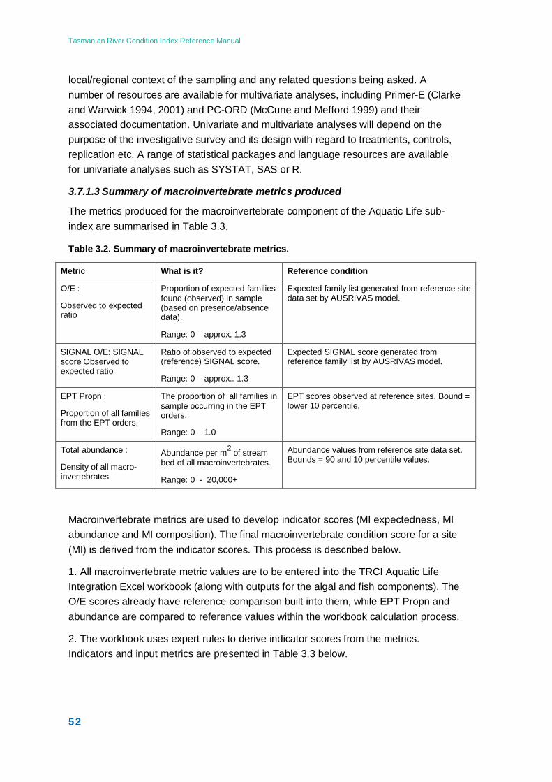
Tasmanian River Condition Index Reference Manual
52
local/regional context of the sampling and any related questions being asked. A number of resources are available for multivariate analyses, including Primer-E (Clarke and Warwick 1994, 2001) and PC-ORD (McCune and Mefford 1999) and their associated documentation. Univariate and multivariate analyses will depend on the purpose of the investigative survey and its design with regard to treatments, controls, replication etc. A range of statistical packages and language resources are available for univariate analyses such as SYSTAT, SAS or R.
3.7.1.3 Summary of macroinvertebrate metrics produced
The metrics produced for the macroinvertebrate component of the Aquatic Life sub-index are summarised in Table 3.3.
Table 3.2. Summary of macroinvertebrate metrics.
Metric What is it? Reference condition
O/E :
Observed to expected ratio
Proportion of expected families found (observed) in sample (based on presence/absence data).
Range: 0 – approx. 1.3
Expected family list generated from reference site data set by AUSRIVAS model.
SIGNAL O/E: SIGNAL score Observed to expected ratio
Ratio of observed to expected (reference) SIGNAL score.
Range: 0 – approx.. 1.3
Expected SIGNAL score generated from reference family list by AUSRIVAS model.
EPT Propn :
Proportion of all families from the EPT orders.
The proportion of all families in sample occurring in the EPT orders.
Range: 0 – 1.0
EPT scores observed at reference sites. Bound = lower 10 percentile.
Total abundance :
Density of all macro-invertebrates
Abundance per m2 of stream bed of all macroinvertebrates.
Range: 0 - 20,000+
Abundance values from reference site data set. Bounds = 90 and 10 percentile values.
Macroinvertebrate metrics are used to develop indicator scores (MI expectedness, MI abundance and MI composition). The final macroinvertebrate condition score for a site (MI) is derived from the indicator scores. This process is described below.
1. All macroinvertebrate metric values are to be entered into the TRCI Aquatic Life Integration Excel workbook (along with outputs for the algal and fish components). The O/E scores already have reference comparison built into them, while EPT Propn and abundance are compared to reference values within the workbook calculation process.
2. The workbook uses expert rules to derive indicator scores from the metrics. Indicators and input metrics are presented in Table 3.3 below.
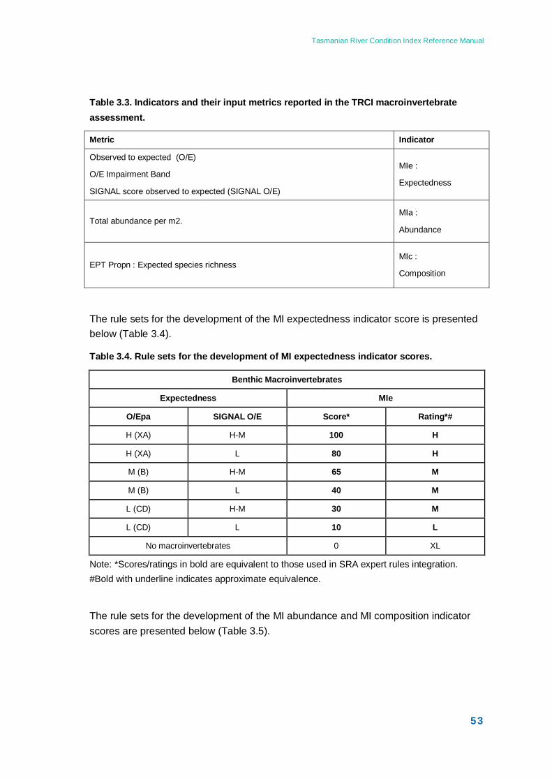
Tasmanian River Condition Index Reference Manual
53
Table 3.3. Indicators and their input metrics reported in the TRCI macroinvertebrate assessment.
Metric Indicator
Observed to expected (O/E)
O/E Impairment Band
SIGNAL score observed to expected (SIGNAL O/E)
MIe :
Expectedness
Total abundance per m2. MIa :
Abundance
EPT Propn : Expected species richness MIc :
Composition
The rule sets for the development of the MI expectedness indicator score is presented below (Table 3.4).
Table 3.4. Rule sets for the development of MI expectedness indicator scores.
Benthic Macroinvertebrates
Expectedness MIe
O/Epa SIGNAL O/E Score* Rating*#
H (XA) H-M 100 H
H (XA) L 80 H
M (B) H-M 65 M
M (B) L 40 M
L (CD) H-M 30 M
L (CD) L 10 L
No macroinvertebrates 0 XL
Note: *Scores/ratings in bold are equivalent to those used in SRA expert rules integration. #Bold with underline indicates approximate equivalence.
The rule sets for the development of the MI abundance and MI composition indicator scores are presented below (Table 3.5).
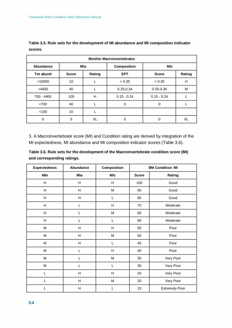
Tasmanian River Condition Index Reference Manual
54
Table 3.5. Rule sets for the development of MI abundance and MI composition indicator scores.
Benthic Macroinvertebrates
Abundance Mia Composition MIc
Tot abund Score Rating EPT Score Rating
>10000 10 L > 0.35 > 0.35 H
>4400 40 L 0.25-0.34 0.25-0.34 M
700 - 4400 100 H 0.15 - 0.24 0.15 - 0.24 L
<700 40 L 0 0 L
<100 10 L
0 0 XL 0 0 XL
3. A Macroinvertebrate score (MI) and Condition rating are derived by integration of the MI expectedness, MI abundance and MI composition indicator scores (Table 3.6).
Table 3.6. Rule sets for the development of the Macroinvertebrate condition score (MI) and corresponding ratings.
Expectedness Abundance Composition BM Condition: MI
MIe MIa MIc Score Rating
H H H 100 Good
H H M 90 Good
H H L 80 Good
H L H 70 Moderate
H L M 65 Moderate
H L L 60 Moderate
M H H 55 Poor
M H M 50 Poor
M H L 45 Poor
M L H 40 Poor
M L M 35 Very Poor
M L L 30 Very Poor
L H H 25 Very Poor
L H M 20 Very Poor
L H L 15 Extremely Poor
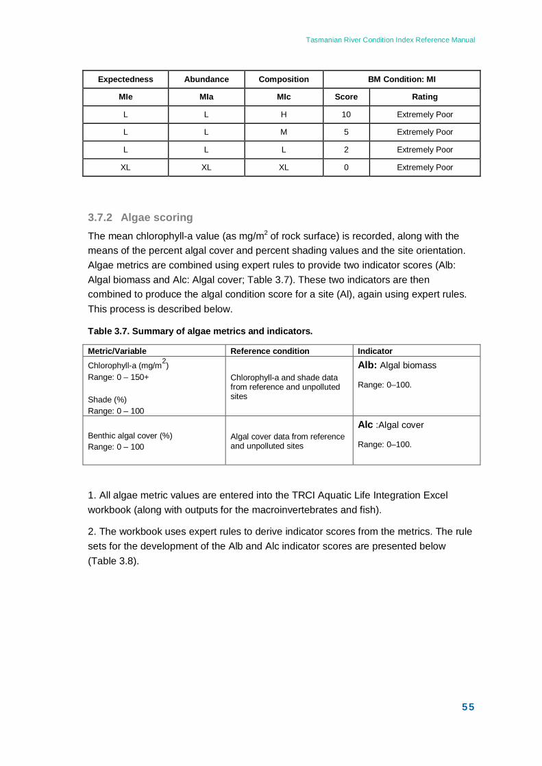
Tasmanian River Condition Index Reference Manual
55
Expectedness Abundance Composition BM Condition: MI
MIe MIa MIc Score Rating
L L H 10 Extremely Poor
L L M 5 Extremely Poor
L L L 2 Extremely Poor
XL XL XL 0 Extremely Poor
3.7.2 Algae scoring The mean chlorophyll-a value (as mg/m2 of rock surface) is recorded, along with the means of the percent algal cover and percent shading values and the site orientation. Algae metrics are combined using expert rules to provide two indicator scores (Alb: Algal biomass and Alc: Algal cover; Table 3.7). These two indicators are then combined to produce the algal condition score for a site (Al), again using expert rules. This process is described below.
Table 3.7. Summary of algae metrics and indicators.
Metric/Variable Reference condition Indicator
Chlorophyll-a (mg/m2) Range: 0 – 150+ Shade (%) Range: 0 – 100
Chlorophyll-a and shade data from reference and unpolluted sites
Alb: Algal biomass
Range: 0–100.
Benthic algal cover (%) Range: 0 – 100
Algal cover data from reference and unpolluted sites
Alc :Algal cover
Range: 0–100.
1. All algae metric values are entered into the TRCI Aquatic Life Integration Excel workbook (along with outputs for the macroinvertebrates and fish).
2. The workbook uses expert rules to derive indicator scores from the metrics. The rule sets for the development of the Alb and Alc indicator scores are presented below (Table 3.8).
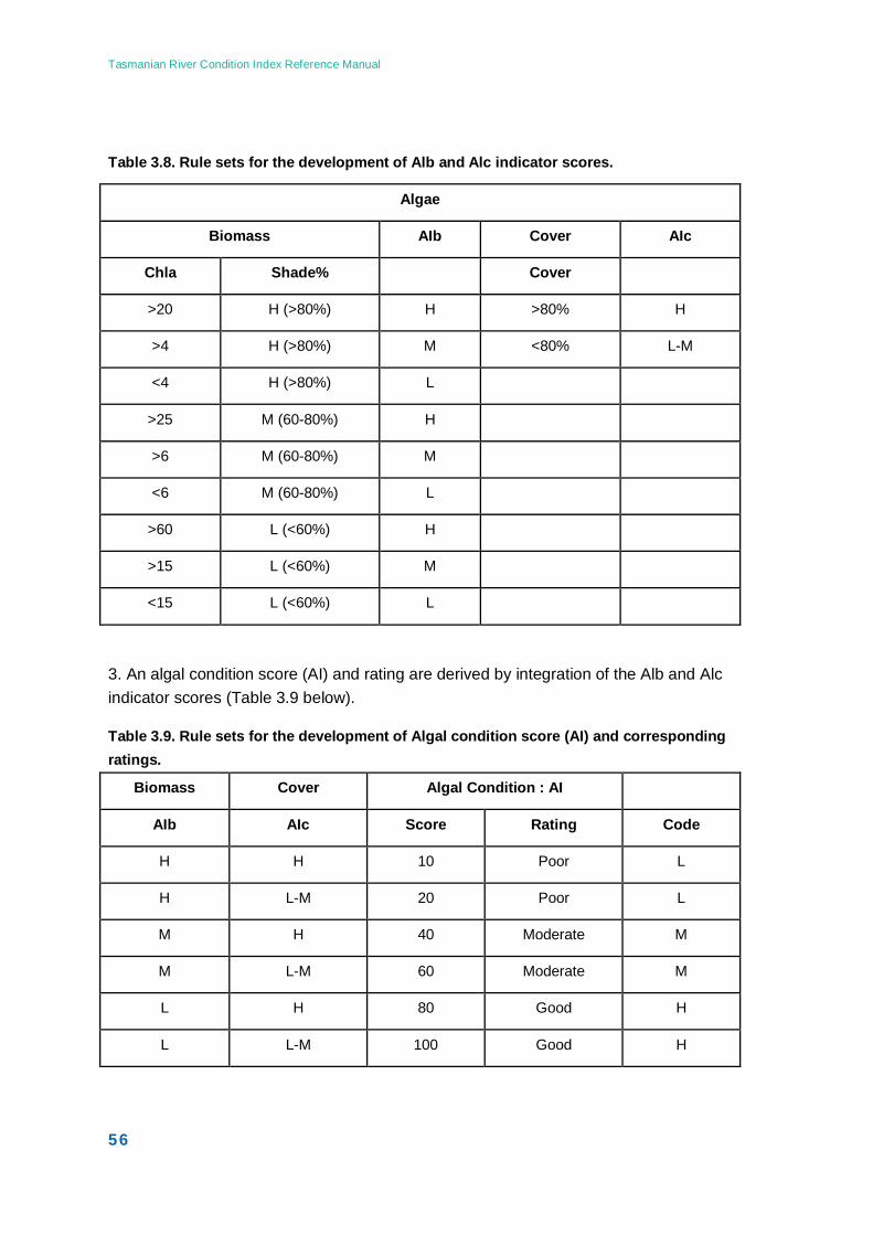
Tasmanian River Condition Index Reference Manual
56
Table 3.8. Rule sets for the development of Alb and Alc indicator scores.
Algae
Biomass AIb Cover AIc
Chla Shade% Cover
>20 H (>80%) H >80% H
>4 H (>80%) M <80% L-M
<4 H (>80%) L
>25 M (60-80%) H
>6 M (60-80%) M
<6 M (60-80%) L
>60 L (<60%) H
>15 L (<60%) M
<15 L (<60%) L
3. An algal condition score (AI) and rating are derived by integration of the Alb and Alc indicator scores (Table 3.9 below).
Table 3.9. Rule sets for the development of Algal condition score (AI) and corresponding ratings.
Biomass Cover Algal Condition : AI
AIb AIc Score Rating Code
H H 10 Poor L
H L-M 20 Poor L
M H 40 Moderate M
M L-M 60 Moderate M
L H 80 Good H
L L-M 100 Good H
Tasmanian River Condition Index Reference Manual
57
3.7.3 Fish scoring 3.7.3.1 Data analysis:
Enter all fish length data, by species, into the Final TRCI AQI Fish Data entry 2009 Excel workbook, as indicated.
You will also need to enter the River Section Catchment identification number (the ‘RSC_id’ attribute) for the river reach within which the sample site was located. This will require interrogating the CFEV Rivers layer, using GIS, locating the river section and obtaining the RSC_id number.
The CFEV river sub-catchment identification number (the ‘SUBCAT_id’ attribute) is also needed to assist in collating the reference species for the subcatchment within which the study site is located. This will require interrogating the CFEV Sub-catchment layer, using GIS, locating the sub-catchment section and obtaining the SUBCAT_id number.
The workbook then calculates:
o the O/E ratio value, as the proportion of the total number of species expected (from CFEV) at the site, that were actually found at the site.
o the O/P ratio value, as the proportion of the total number of species expected (from CFEV) in the sub-catchment, that were actually found at the site. sub-catchment (from CFEV) that were found at the site.
o the biomass for each individual fish, using established length-weight relationships for each species, and derives total biomass for each species, of all native species, and of all exotic species. It then calculates the proportion of species, biomass and of abundance that is composed of native fish.
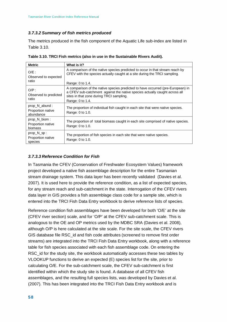
Tasmanian River Condition Index Reference Manual
58
3.7.3.2 Summary of fish metrics produced
The metrics produced in the fish component of the Aquatic Life sub-index are listed in Table 3.10.
Table 3.10. TRCI Fish metrics (also in use in the Sustainable Rivers Audit).
Metric What is it?
O/E : Observed to expected ratio
A comparison of the native species predicted to occur in that stream reach by CFEV with the species actually caught at a site during the TRCI sampling. Range: 0 to 1.4.
O/P : Observed to predicted ratio
A comparison of the native species predicted to have occurred (pre-European) in a CFEV sub-catchment against the native species actually caught across all sites in that zone during TRCI sampling. Range: 0 to 1.4.
prop_N_abund : Proportion native abundance
The proportion of individual fish caught in each site that were native species. Range: 0 to 1.0.
prop_N_biom : Proportion native biomass
The proportion of total biomass caught in each site comprised of native species. Range: 0 to 1.0.
prop_N_sp : Proportion native species
The proportion of fish species in each site that were native species. Range: 0 to 1.0.
3.7.3.3 Reference Condition for Fish
In Tasmania the CFEV (Conservation of Freshwater Ecosystem Values) framework project developed a native fish assemblage description for the entire Tasmanian stream drainage system. This data layer has been recently validated (Davies et al. 2007). It is used here to provide the reference condition, as a list of expected species, for any stream reach and sub-catchment in the state. Interrogation of the CFEV rivers data layer in GIS provides a fish assemblage class code for a sample site, which is entered into the TRCI Fish Data Entry workbook to derive reference lists of species.
Reference condition fish assemblages have been developed for both ‘O/E’ at the site (CFEV river section) scale, and for ‘O/P’ at the CFEV sub-catchment scale. This is analogous to the OE and OP metrics used by the MDBC SRA (Davies et al. 2008), although O/P is here calculated at the site scale. For the site scale, the CFEV rivers GIS database file RSC_id and fish code attributes (screened to remove first order streams) are integrated into the TRCI Fish Data Entry workbook, along with a reference table for fish species associated with each fish assemblage code. On entering the RSC_id for the study site, the workbook automatically accesses these two tables by VLOOKUP functions to derive an expected (E) species list for the site, prior to calculating O/E. For the sub-catchment scale, the CFEV sub-catchment is first identified within which the study site is found. A database of all CFEV fish assemblages, and the resulting full species lists, was developed by Davies et al. (2007). This has been integrated into the TRCI Fish Data Entry workbook and is
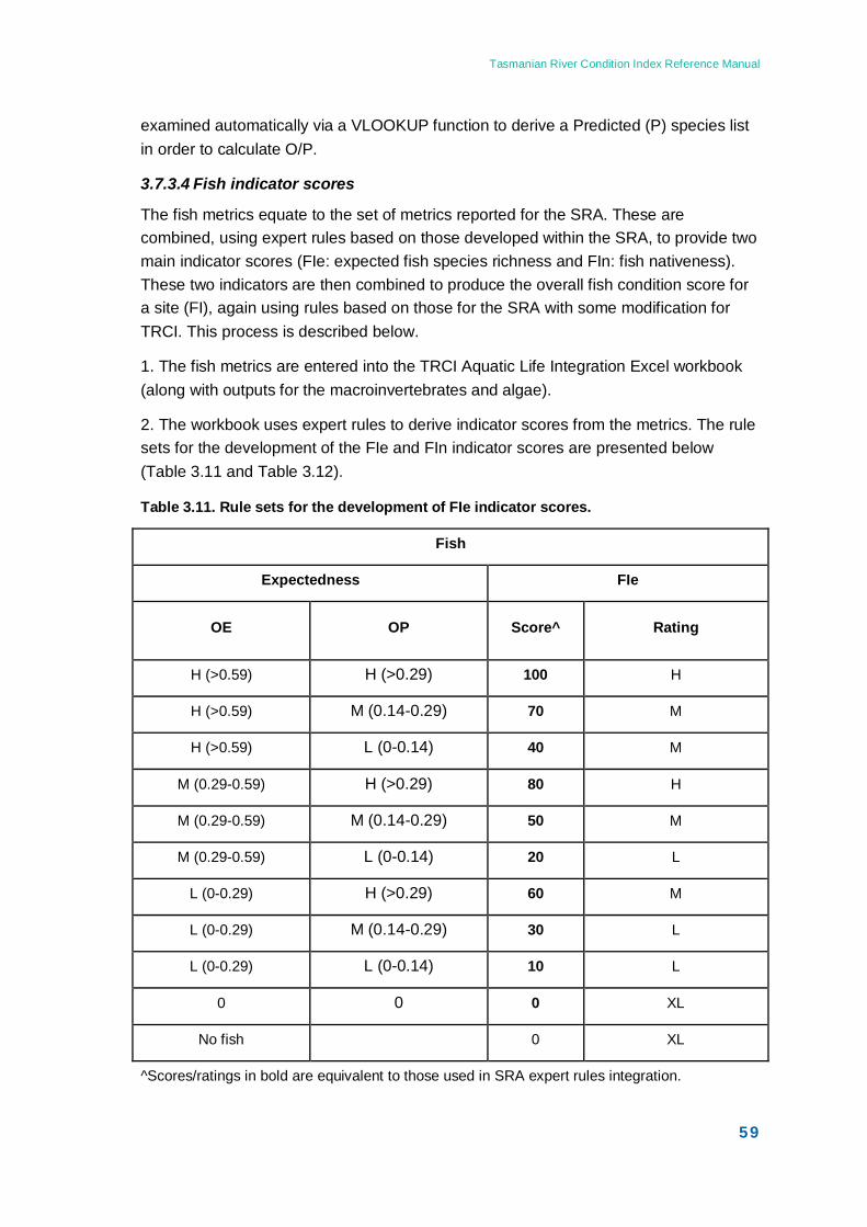
Tasmanian River Condition Index Reference Manual
59
examined automatically via a VLOOKUP function to derive a Predicted (P) species list in order to calculate O/P.
3.7.3.4 Fish indicator scores
The fish metrics equate to the set of metrics reported for the SRA. These are combined, using expert rules based on those developed within the SRA, to provide two main indicator scores (FIe: expected fish species richness and FIn: fish nativeness). These two indicators are then combined to produce the overall fish condition score for a site (FI), again using rules based on those for the SRA with some modification for TRCI. This process is described below.
1. The fish metrics are entered into the TRCI Aquatic Life Integration Excel workbook (along with outputs for the macroinvertebrates and algae).
2. The workbook uses expert rules to derive indicator scores from the metrics. The rule sets for the development of the FIe and FIn indicator scores are presented below (Table 3.11 and Table 3.12).
Table 3.11. Rule sets for the development of FIe indicator scores.
Fish
Expectedness FIe
OE OP Score^ Rating
H (>0.59) H (>0.29) 100 H
H (>0.59) M (0.14-0.29) 70 M
H (>0.59) L (0-0.14) 40 M
M (0.29-0.59) H (>0.29) 80 H
M (0.29-0.59) M (0.14-0.29) 50 M
M (0.29-0.59) L (0-0.14) 20 L
L (0-0.29) H (>0.29) 60 M
L (0-0.29) M (0.14-0.29) 30 L
L (0-0.29) L (0-0.14) 10 L
0 0 0 XL
No fish 0 XL
^Scores/ratings in bold are equivalent to those used in SRA expert rules integration.
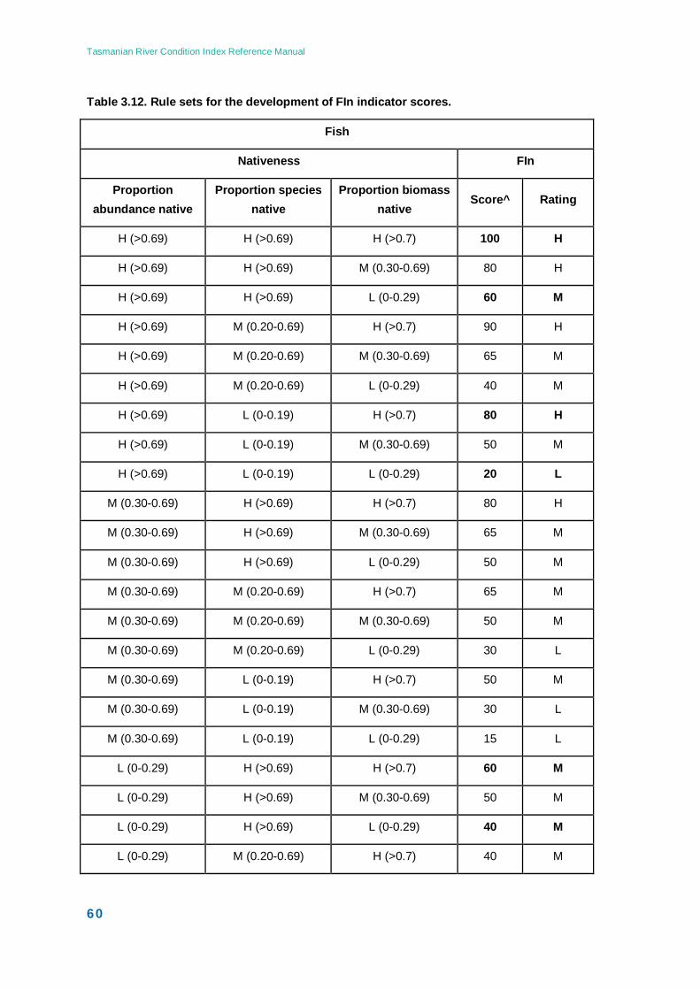
Tasmanian River Condition Index Reference Manual
60
Table 3.12. Rule sets for the development of FIn indicator scores.
Fish
Nativeness FIn
Proportion abundance native
Proportion species native
Proportion biomass native
Score^ Rating
H (>0.69) H (>0.69) H (>0.7) 100 H
H (>0.69) H (>0.69) M (0.30-0.69) 80 H
H (>0.69) H (>0.69) L (0-0.29) 60 M
H (>0.69) M (0.20-0.69) H (>0.7) 90 H
H (>0.69) M (0.20-0.69) M (0.30-0.69) 65 M
H (>0.69) M (0.20-0.69) L (0-0.29) 40 M
H (>0.69) L (0-0.19) H (>0.7) 80 H
H (>0.69) L (0-0.19) M (0.30-0.69) 50 M
H (>0.69) L (0-0.19) L (0-0.29) 20 L
M (0.30-0.69) H (>0.69) H (>0.7) 80 H
M (0.30-0.69) H (>0.69) M (0.30-0.69) 65 M
M (0.30-0.69) H (>0.69) L (0-0.29) 50 M
M (0.30-0.69) M (0.20-0.69) H (>0.7) 65 M
M (0.30-0.69) M (0.20-0.69) M (0.30-0.69) 50 M
M (0.30-0.69) M (0.20-0.69) L (0-0.29) 30 L
M (0.30-0.69) L (0-0.19) H (>0.7) 50 M
M (0.30-0.69) L (0-0.19) M (0.30-0.69) 30 L
M (0.30-0.69) L (0-0.19) L (0-0.29) 15 L
L (0-0.29) H (>0.69) H (>0.7) 60 M
L (0-0.29) H (>0.69) M (0.30-0.69) 50 M
L (0-0.29) H (>0.69) L (0-0.29) 40 M
L (0-0.29) M (0.20-0.69) H (>0.7) 40 M
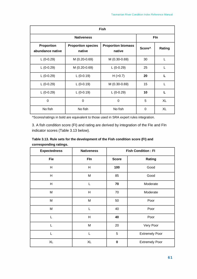
Tasmanian River Condition Index Reference Manual
61
Fish
Nativeness FIn
Proportion abundance native
Proportion species native
Proportion biomass native
Score^ Rating
L (0-0.29) M (0.20-0.69) M (0.30-0.69) 30 L
L (0-0.29) M (0.20-0.69) L (0-0.29) 25 L
L (0-0.29) L (0-0.19) H (>0.7) 20 L
L (0-0.29) L (0-0.19) M (0.30-0.69) 15 L
L (0-0.29) L (0-0.19) L (0-0.29) 10 L
0 0 0 5 XL
No fish No fish No fish 0 XL
^Scores/ratings in bold are equivalent to those used in SRA expert rules integration.
3. A fish condition score (FI) and rating are derived by integration of the FIe and FIn indicator scores (Table 3.13 below).
Table 3.13. Rule sets for the development of the Fish condition score (FI) and corresponding ratings.
Expectedness Nativeness Fish Condition : FI
Fie FIn Score Rating
H H 100 Good
H M 85 Good
H L 70 Moderate
M H 70 Moderate
M M 50 Poor
M L 40 Poor
L H 40 Poor
L M 20 Very Poor
L L 5 Extremely Poor
XL XL 0 Extremely Poor
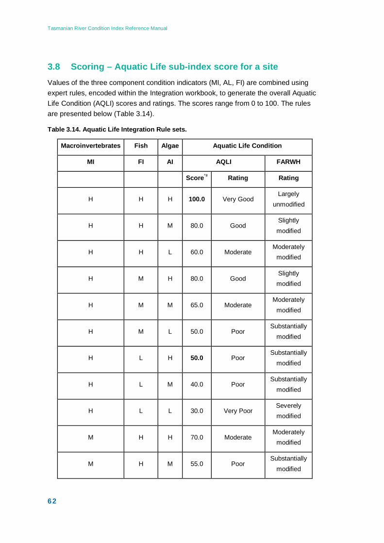
Tasmanian River Condition Index Reference Manual
62
3.8 Scoring – Aquatic Life sub-index score for a site Values of the three component condition indicators (MI, AL, FI) are combined using expert rules, encoded within the Integration workbook, to generate the overall Aquatic Life Condition (AQLI) scores and ratings. The scores range from 0 to 100. The rules are presented below (Table 3.14).
Table 3.14. Aquatic Life Integration Rule sets.
Macroinvertebrates Fish Algae Aquatic Life Condition
MI FI AI AQLI FARWH
Score*# Rating Rating
H H H 100.0 Very Good Largely
unmodified
H H M 80.0 Good Slightly modified
H H L 60.0 Moderate Moderately
modified
H M H 80.0 Good Slightly modified
H M M 65.0 Moderate Moderately
modified
H M L 50.0 Poor Substantially
modified
H L H 50.0 Poor Substantially
modified
H L M 40.0 Poor Substantially
modified
H L L 30.0 Very Poor Severely modified
M H H 70.0 Moderate Moderately
modified
M H M 55.0 Poor Substantially
modified
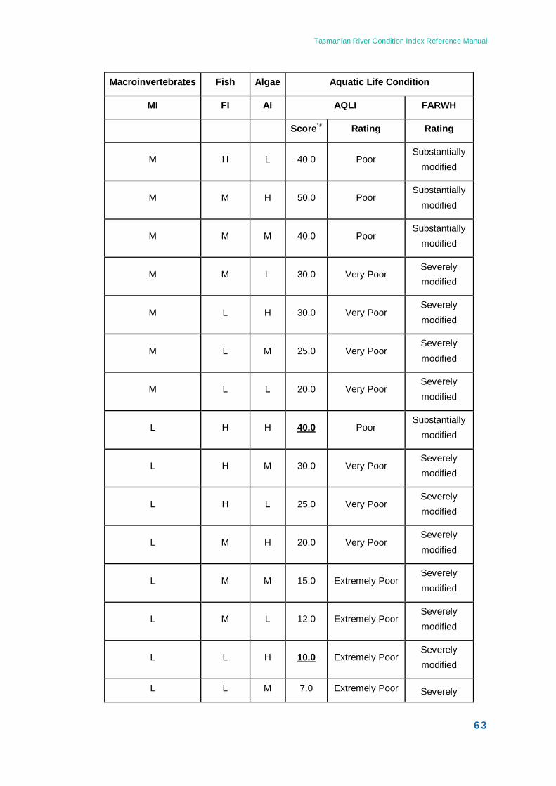
Tasmanian River Condition Index Reference Manual
63
Macroinvertebrates Fish Algae Aquatic Life Condition
MI FI AI AQLI FARWH
Score*# Rating Rating
M H L 40.0 Poor Substantially
modified
M M H 50.0 Poor Substantially
modified
M M M 40.0 Poor Substantially
modified
M M L 30.0 Very Poor Severely modified
M L H 30.0 Very Poor Severely modified
M L M 25.0 Very Poor Severely modified
M L L 20.0 Very Poor Severely modified
L H H Poor 40.0 Substantially
modified
L H M 30.0 Very Poor Severely modified
L H L 25.0 Very Poor Severely modified
L M H 20.0 Very Poor Severely modified
L M M 15.0 Extremely Poor Severely modified
L M L 12.0 Extremely Poor Severely modified
L L H Extremely Poor 10.0 Severely modified
L L M 7.0 Extremely Poor Severely
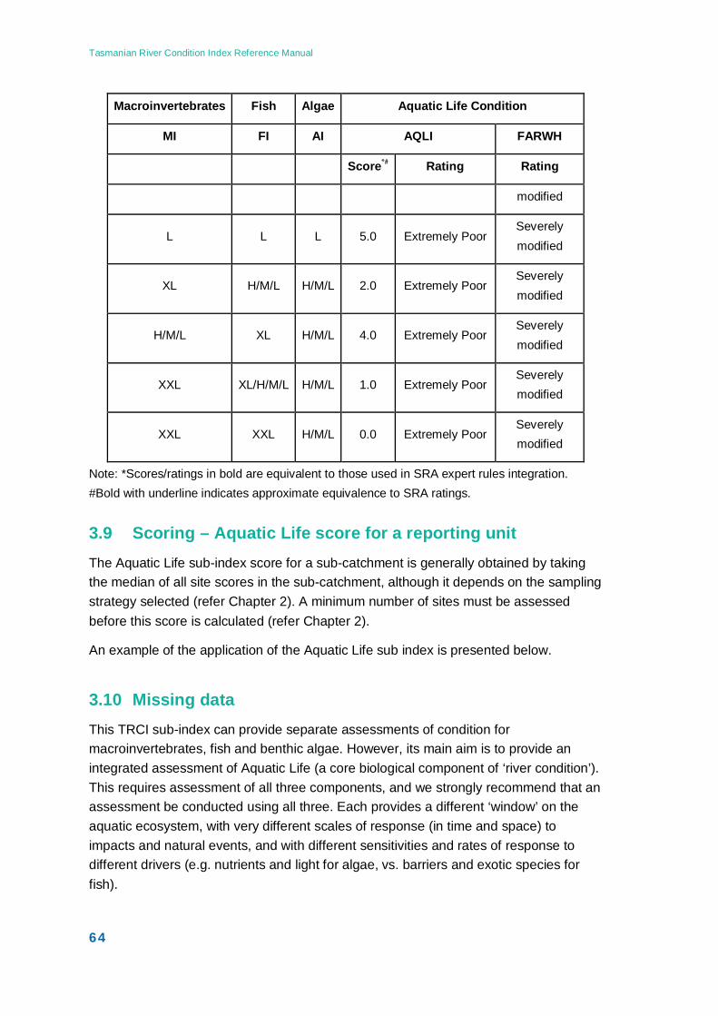
Tasmanian River Condition Index Reference Manual
64
Macroinvertebrates Fish Algae Aquatic Life Condition
MI FI AI AQLI FARWH
Score*# Rating Rating
modified
L L L 5.0 Extremely Poor Severely modified
XL H/M/L H/M/L 2.0 Extremely Poor Severely modified
H/M/L XL H/M/L 4.0 Extremely Poor Severely modified
XXL XL/H/M/L H/M/L 1.0 Extremely Poor Severely modified
XXL XXL H/M/L 0.0 Extremely Poor Severely modified
Note: *Scores/ratings in bold are equivalent to those used in SRA expert rules integration. #Bold with underline indicates approximate equivalence to SRA ratings.
3.9 Scoring – Aquatic Life score for a reporting unit The Aquatic Life sub-index score for a sub-catchment is generally obtained by taking the median of all site scores in the sub-catchment, although it depends on the sampling strategy selected (refer Chapter 2). A minimum number of sites must be assessed before this score is calculated (refer Chapter 2).
An example of the application of the Aquatic Life sub index is presented below.
3.10 Missing data This TRCI sub-index can provide separate assessments of condition for macroinvertebrates, fish and benthic algae. However, its main aim is to provide an integrated assessment of Aquatic Life (a core biological component of ‘river condition’). This requires assessment of all three components, and we strongly recommend that an assessment be conducted using all three. Each provides a different ‘window’ on the aquatic ecosystem, with very different scales of response (in time and space) to impacts and natural events, and with different sensitivities and rates of response to different drivers (e.g. nutrients and light for algae, vs. barriers and exotic species for fish).
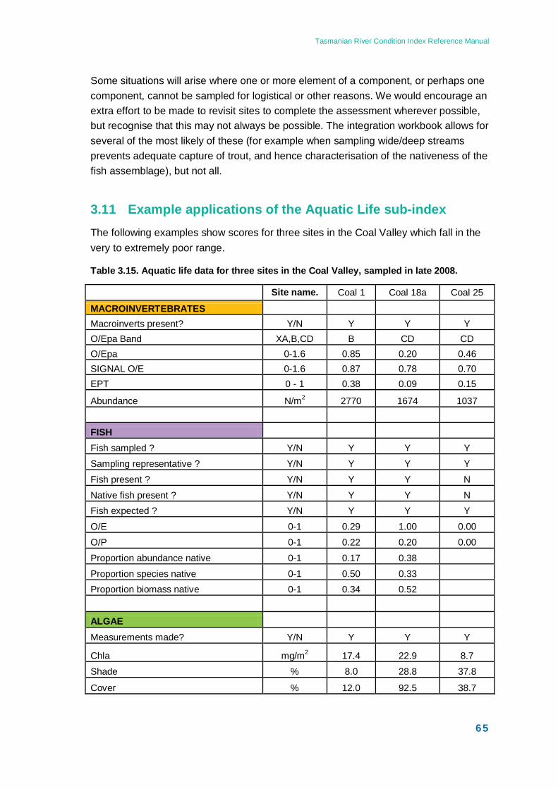
Tasmanian River Condition Index Reference Manual
65
Some situations will arise where one or more element of a component, or perhaps one component, cannot be sampled for logistical or other reasons. We would encourage an extra effort to be made to revisit sites to complete the assessment wherever possible, but recognise that this may not always be possible. The integration workbook allows for several of the most likely of these (for example when sampling wide/deep streams prevents adequate capture of trout, and hence characterisation of the nativeness of the fish assemblage), but not all.
3.11 Example applications of the Aquatic Life sub-index The following examples show scores for three sites in the Coal Valley which fall in the very to extremely poor range.
Table 3.15. Aquatic life data for three sites in the Coal Valley, sampled in late 2008.
Site name. Coal 1 Coal 18a Coal 25
MACROINVERTEBRATES Macroinverts present? Y/N Y Y Y O/Epa Band XA,B,CD B CD CD O/Epa 0-1.6 0.85 0.20 0.46 SIGNAL O/E 0-1.6 0.87 0.78 0.70 EPT 0 - 1 0.38 0.09 0.15
Abundance N/m2 2770 1674 1037
FISH Fish sampled ? Y/N Y Y Y
Sampling representative ? Y/N Y Y Y
Fish present ? Y/N Y Y N
Native fish present ? Y/N Y Y N Fish expected ? Y/N Y Y Y
O/E 0-1 0.29 1.00 0.00
O/P 0-1 0.22 0.20 0.00
Proportion abundance native 0-1 0.17 0.38
Proportion species native 0-1 0.50 0.33 Proportion biomass native 0-1 0.34 0.52
ALGAE
Measurements made? Y/N Y Y Y
Chla mg/m2 17.4 22.9 8.7
Shade % 8.0 28.8 37.8
Cover % 12.0 92.5 38.7
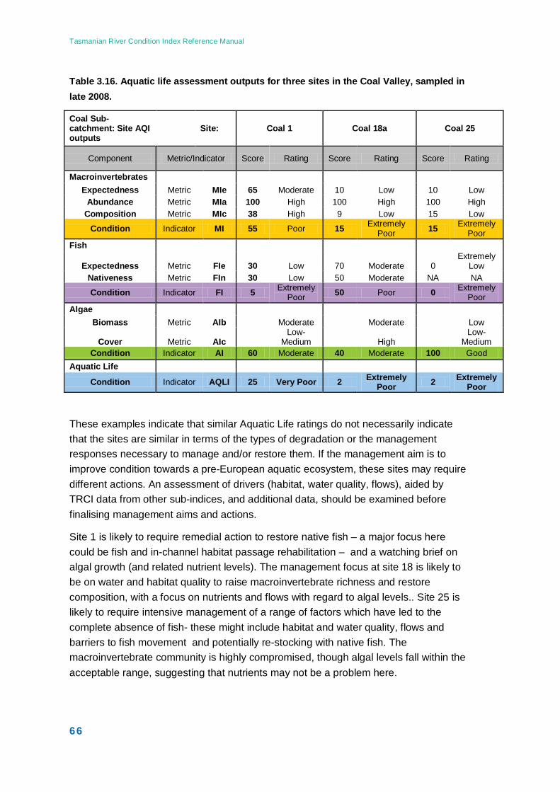
Tasmanian River Condition Index Reference Manual
66
Table 3.16. Aquatic life assessment outputs for three sites in the Coal Valley, sampled in late 2008.
Coal Sub-catchment: Site AQI outputs
Site: Coal 1 Coal 18a Coal 25
Component Metric/Indicator Score Rating Score Rating Score Rating
Macroinvertebrates Expectedness Metric MIe 65 Moderate 10 Low 10 Low
Abundance Metric MIa 100 High 100 High 100 High Composition Metric MIc 38 High 9 Low 15 Low
Condition Indicator MI 55 Poor 15 Extremely Poor 15 Extremely
Poor Fish
Expectedness Metric FIe 30 Low 70 Moderate 0 Extremely
Low Nativeness Metric FIn 30 Low 50 Moderate NA NA
Condition Indicator FI 5 Extremely Poor 50 Poor 0 Extremely
Poor Algae
Biomass Metric AIb Moderate Moderate Low
Cover Metric AIc Low-
Medium High Low-
Medium Condition Indicator AI 60 Moderate 40 Moderate 100 Good
Aquatic Life
Condition Indicator AQLI 25 Very Poor 2 Extremely Poor 2 Extremely
Poor
These examples indicate that similar Aquatic Life ratings do not necessarily indicate that the sites are similar in terms of the types of degradation or the management responses necessary to manage and/or restore them. If the management aim is to improve condition towards a pre-European aquatic ecosystem, these sites may require different actions. An assessment of drivers (habitat, water quality, flows), aided by TRCI data from other sub-indices, and additional data, should be examined before finalising management aims and actions.
Site 1 is likely to require remedial action to restore native fish – a major focus here could be fish and in-channel habitat passage rehabilitation – and a watching brief on algal growth (and related nutrient levels). The management focus at site 18 is likely to be on water and habitat quality to raise macroinvertebrate richness and restore composition, with a focus on nutrients and flows with regard to algal levels.. Site 25 is likely to require intensive management of a range of factors which have led to the complete absence of fish- these might include habitat and water quality, flows and barriers to fish movement and potentially re-stocking with native fish. The macroinvertebrate community is highly compromised, though algal levels fall within the acceptable range, suggesting that nutrients may not be a problem here.
Tasmanian River Condition Index Reference Manual
67
3.12 References - Aquatic Life APHA (2005) Standard Methods for the Examination of Water and Wastewater, 21st Edition. American Public Health Association (APHA), American Water Works Association (AWWA) & Water Environment Federation (WEF).
Chessman BC (2003) New sensitivity grades for Australian river macroinvertebrates. Marine and Freshwater Research 54, 95 - 103.
Clarke KR and Warwick RM (1994). Change in marine communities: an approach to statistical analysis and interpretation. Plymouth Marine Laboratory, Plymouth UK.
Davies, PE, Cook, LSJ, Koehnken, L and Barker P (2007) National Water Initiative - Australian Government Water Fund: Validation of the Conservation of Freshwater Ecosystem Values (CFEV) Framework. Report to Water Resources Division, DPIW, Hobart 76 pp.
Davies PE, Hillman TJ, Harris JH and Walker KF (2008). The Sustainable Rivers Audit (SRA): River Health Check. Report 1. Independent Sustainable Rivers Audit Group, Murray– Darling Basin Ministerial Council. Technical Report. Murray–Darling Basin Commission, ACT. May 2008.
Davies, P.E. (2009) Tasmanian River Condition Index: Phase 3 Aquatic Life Sampling Results, Analysis and Recommendations for the final TRCI method. A report to NRM South, Hobart.
DPIW (2008) Conservation of Freshwater Ecosystem Values (CFEV) project Technical Report. Conservation of Freshwater Ecosystem Values Program. Department of Primary Industries and Water, Hobart, Tasmania. 227 pp.
Gooderham, J, Barmuta, LA and Davies, PE (2007). Upstream heterogeneous zones: small stream systems structured by a lack of competence? Journal of the North American Benthological Society, 26, 365-374.
Hawkins C, Ostermiller J, Vinson M, and Stevenson RJ (2001) Stream algae, invertebrate, and environmental sampling associated with biological water quality assessments: Field Protocols. Utah State University, Logan, Utah 84322-5210. 11 May 2001. 23 pp. ://www1.usu.edu/buglab/monitor/USUproto.pdf
Krasnicki T, Pinto R and Read M (2001) Australia Wide Assessment of River Health. Final Report. DPIWE Water Assessment Branch, Hobart. Report Series WRA 01/2001. 171 pp.
Marchant, R. (1989) A subsampler for samples of benthic macroinvertebrates. Bulletin of the Australian Society for Limnology 12, 49-52.
McCune B and Mefford MJ, (1999) PC-ORD. Multivariate Analysis of Ecological Data, Version 4. MjM Software Design: Gleneden Beach, OR, USA.

Tasmanian River Condition Index Reference Manual
68
MDBC (2004) A six year working program for the design and implementation of the Sustainable Rivers Audit. MDBC, Canberra
NSW Fisheries (1997) The Australian Code of Electrofishing Practice. NSW Fisheries Management Publication No. 1. 14pp.

Tasmanian River Condition Index Reference Manual
69

Tasmanian River Condition Index Reference Manual
70
Appendix to Chapter 3: Further detail on the Aquatic Life sub-index Appendix 3.1 The Development of Aquatic Life Reference Conditions
Tasmanian River Condition Index Reference Manual
71
Appendix 3.1 The development of Aquatic Life reference conditions
Macroinvertebrates Macroinvertebrate EPT
A set of reference EPT metric scores were derived by calculating the proportion of all AUSRIVAS families within the EPT orders for all reference site riffle habitat kick samples used in deriving AUSRIVAS models (data sourced from DPIW, Tasmania). A total of 222 reference sample EPT values were used, with a mean of 0.43 and range of 0.33 – 0.64, to define a lower (10th percentile) bound for the reference condition = 0.347. A lower limit for EPT of 0.35 was used to define the cut-off for samples that were equivalent to reference for this metric.
Therefore, samples with EPT values > 0.35 were deemed equivalent to reference, and those with values between 0.25 and 0.35 were deemed to have a significant deviation from reference, while values < 0.15 were rated as having a substantial deviation from reference (and equated, respectively, to Mid and Low ratings in the macroinvertebrate integration rule set).
The definition of reference for EPT is relatively crude and could be improved. The use of AUSRIVAS model reference site classification groupings as the basis for this refinement is not recommended, as those groupings are based on assemblage data in which all taxa are equivalent, and do not represent regional variation in reference EPT values well (Davies unpub. data). A CART regression tree analysis of EPT values was conducted for AUSRIVAS reference sites for this project. The tree analysis was statistically significant and results could be used to develop a rule-based regionalisation of EPT reference threshold values. However, they have not been adopted into the TRCI yet as the justification for additional complexity in reference calculation relative to the responsiveness of the metric has yet to be demonstrated. Work is ongoing in this area (contact P. Davies for more information, [email protected]).
Macroinvertebrate abundance
All quantitative riffle habitat benthic macroinvertebrate data available within the state (primarily from Surber sampling) were collated, sourced from a wide variety of monitoring programs and published and unpublished research projects. A total of 322 quantitative estimates of macroinvertebrate abundance (as n/m2) were sourced, for known reference sites and sites with minimal known human impacts, from 18 separate studies (177 sites) distributed widely across the state (53, 57 and 6 sites in the northeast, west and south of the state respectively). Each estimate was based on at least 5 pooled Surber samples, with over 90% based on 10 – 15 pooled samples.
Tasmanian River Condition Index Reference Manual
72
Values ranged from 96 to 17,978 individuals per m2. Lower and upper bounds were defined based on the 10th and 90th percentiles of this data distribution – 723 and 4,404 per m2.
No relationship was found between abundance values and elevation, stream order or hydrological region, by correlation or analysis of variance. A significant difference (by one way ANOVA, p < 0.002) was found in abundance between ‘western’ sites – from all northern, north-western and western catchments between the Mersey westward and southward to the upper Derwent catchment – and ‘northeastern’ sites – from all catchments from the Tamar eastward to the Apsley catchment. ‘Western’ sites had a mean abundance of 2158 per m2 (n = 170) while north-eastern sites had a mean abundance of 2774 per m2 (n = 142).
This analysis indicated that there are regional differences in reference macroinvertebrate abundance levels. However, the limited amount of southern and south-eastern data prevented a full regionalisation of the reference abundance data. The default values identified above were therefore used to define a preliminary abundance reference range for the state.
A set of quantitative abundance values from known impaired sites was assembled (n = 315). Of these, 175 (56%) were found to fall either above or below the 90th and 10th percentile values, respectively, derived from the reference data set. The distribution of these values along with reference values are shown in Figure A3.1. 1.
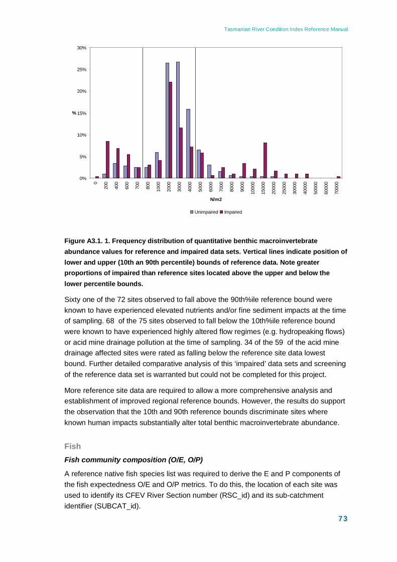
Tasmanian River Condition Index Reference Manual
73
Figure A3.1. 1. Frequency distribution of quantitative benthic macroinvertebrate abundance values for reference and impaired data sets. Vertical lines indicate position of lower and upper (10th an 90th percentile) bounds of reference data. Note greater proportions of impaired than reference sites located above the upper and below the lower percentile bounds.
Sixty one of the 72 sites observed to fall above the 90th%ile reference bound were known to have experienced elevated nutrients and/or fine sediment impacts at the time of sampling. 68 of the 75 sites observed to fall below the 10th%ile reference bound were known to have experienced highly altered flow regimes (e.g. hydropeaking flows) or acid mine drainage pollution at the time of sampling. 34 of the 59 of the acid mine drainage affected sites were rated as falling below the reference site data lowest bound. Further detailed comparative analysis of this ‘impaired’ data sets and screening of the reference data set is warranted but could not be completed for this project.
More reference site data are required to allow a more comprehensive analysis and establishment of improved regional reference bounds. However, the results do support the observation that the 10th and 90th reference bounds discriminate sites where known human impacts substantially alter total benthic macroinvertebrate abundance.
Fish Fish community composition (O/E, O/P)
A reference native fish species list was required to derive the E and P components of the fish expectedness O/E and O/P metrics. To do this, the location of each site was used to identify its CFEV River Section number (RSC_id) and its sub-catchment identifier (SUBCAT_id).
0%
5%
10%
15%
20%
25%
30%
0
200
400
600
700
800
1000
2000
3000
4000
5000
6000
7000
8000
9000
1000
0
1500
0
2000
0
2500
0
3000
0
4000
0
5000
0
6000
0
7000
0
N/m2
%
Unimpaired Impaired
Tasmanian River Condition Index Reference Manual
74
The RSC_id was used to identify the CFEV native fish assemblage relevant to the site. This was matched to the species list documented in CFEV, to derive a list of expected species for the site.
The proportion of this expected species list that was actually observed at a site was then calculated as the O/E metric.
The SUBCAT_id was used to identify all CFEV native fish assemblages occurring in river sections within it. This was then used to compile a full species list for the subcatchment.
The proportion of this predicted species list that was actually observed at a site was then calculated as the O/P metric.
It was recognised that the rules used to model the CFEV species assemblages could miss individual species occurrences within or close to the limits of the species’ ranges. Any native fish species found at a site was therefore deemed to be expected, and added to the expected and predicted species lists before calculating the O/E and O/P metric values.
This has the inherent property of over-estimating the metrics where native species have been translocated within Tasmania. However, the knowledge of this is limited, with the exception of Galaxias maculatus in and adjacent to Lake Crescent, Tooms Lake and some locations in the Macquarie River. In addition, blackfish (Gadopsis marmoratus) is believed to not occur naturally in the South Esk catchment. There is no scientific basis to this belief, and an accumulation of observations of this species in the Meander and Macquarie Rivers may suggest that this is not the case.
Overall, it is believed that inclusion of all observed native fish species in the reference for calculating O/E and O/P is justified as correcting for errors in distributional absences in the CFEV framework is likely to outweigh the low frequency of occurrence of translocated native fish within the state. However, users will need to be aware of cases where translocation occurs and apply this knowledge when finalising metric scores.
The use of CFEV species assemblage data and fish rule sets was tested using new fish survey data collected in March 2009 for DPIW World Heritage Area management (Davies, Robinson and Driessen, report in prep). 28 stream sites in pristine coastal catchments of the Tasmanian World Heritage Area between Macquarie Harbour and South Cape were surveyed using the TRCI fish method. None of these sites contained alien fish species, and the native fish assemblages were therefore assumed to be in reference condition. TRCI ratings for each site were examined, and also examined after removal of between 1 and 5 species from each data set. All sites rated High for the O/E metric when the true survey data was entered, and rating performance was also deemed suitable as species were removed from the data. Thresholds for the rule set for rating O/P were adjusted to ensure that all survey sites rated High when the true
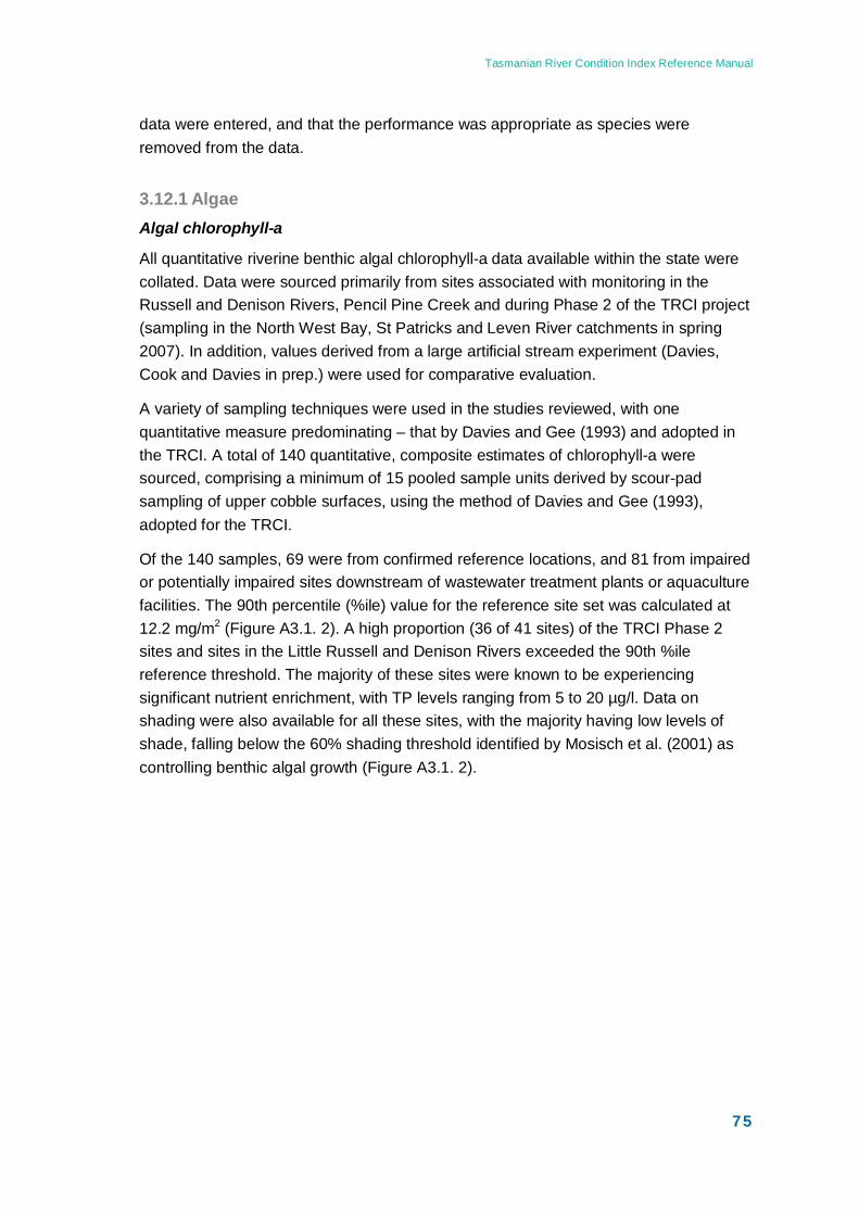
Tasmanian River Condition Index Reference Manual
75
data were entered, and that the performance was appropriate as species were removed from the data.
3.12.1 Algae Algal chlorophyll-a
All quantitative riverine benthic algal chlorophyll-a data available within the state were collated. Data were sourced primarily from sites associated with monitoring in the Russell and Denison Rivers, Pencil Pine Creek and during Phase 2 of the TRCI project (sampling in the North West Bay, St Patricks and Leven River catchments in spring 2007). In addition, values derived from a large artificial stream experiment (Davies, Cook and Davies in prep.) were used for comparative evaluation.
A variety of sampling techniques were used in the studies reviewed, with one quantitative measure predominating – that by Davies and Gee (1993) and adopted in the TRCI. A total of 140 quantitative, composite estimates of chlorophyll-a were sourced, comprising a minimum of 15 pooled sample units derived by scour-pad sampling of upper cobble surfaces, using the method of Davies and Gee (1993), adopted for the TRCI.
Of the 140 samples, 69 were from confirmed reference locations, and 81 from impaired or potentially impaired sites downstream of wastewater treatment plants or aquaculture facilities. The 90th percentile (%ile) value for the reference site set was calculated at 12.2 mg/m2 (Figure A3.1. 2). A high proportion (36 of 41 sites) of the TRCI Phase 2 sites and sites in the Little Russell and Denison Rivers exceeded the 90th %ile reference threshold. The majority of these sites were known to be experiencing significant nutrient enrichment, with TP levels ranging from 5 to 20 µg/l. Data on shading were also available for all these sites, with the majority having low levels of shade, falling below the 60% shading threshold identified by Mosisch et al. (2001) as controlling benthic algal growth (Figure A3.1. 2).
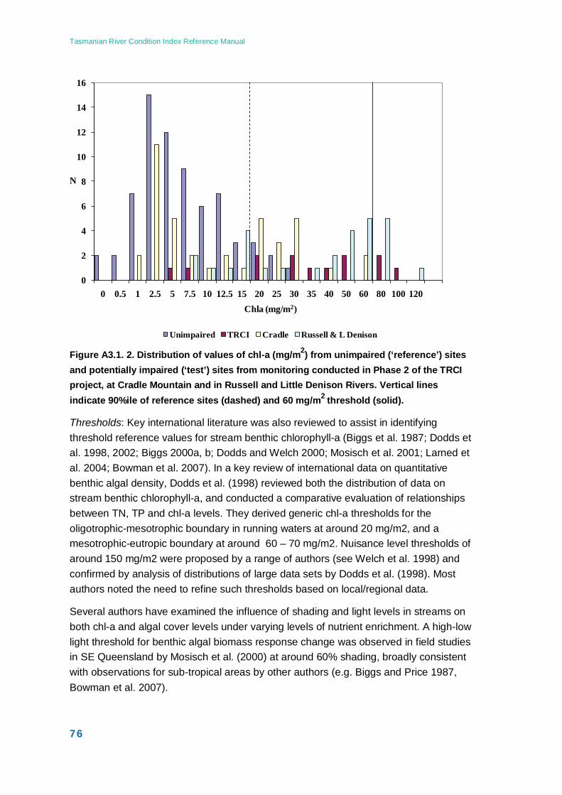
Tasmanian River Condition Index Reference Manual
76
Figure A3.1. 2. Distribution of values of chl-a (mg/m2) from unimpaired (‘reference’) sites and potentially impaired (‘test’) sites from monitoring conducted in Phase 2 of the TRCI project, at Cradle Mountain and in Russell and Little Denison Rivers. Vertical lines indicate 90%ile of reference sites (dashed) and 60 mg/m2 threshold (solid).
Thresholds: Key international literature was also reviewed to assist in identifying threshold reference values for stream benthic chlorophyll-a (Biggs et al. 1987; Dodds et al. 1998, 2002; Biggs 2000a, b; Dodds and Welch 2000; Mosisch et al. 2001; Larned et al. 2004; Bowman et al. 2007). In a key review of international data on quantitative benthic algal density, Dodds et al. (1998) reviewed both the distribution of data on stream benthic chlorophyll-a, and conducted a comparative evaluation of relationships between TN, TP and chl-a levels. They derived generic chl-a thresholds for the oligotrophic-mesotrophic boundary in running waters at around 20 mg/m2, and a mesotrophic-eutropic boundary at around 60 – 70 mg/m2. Nuisance level thresholds of around 150 mg/m2 were proposed by a range of authors (see Welch et al. 1998) and confirmed by analysis of distributions of large data sets by Dodds et al. (1998). Most authors noted the need to refine such thresholds based on local/regional data.
Several authors have examined the influence of shading and light levels in streams on both chl-a and algal cover levels under varying levels of nutrient enrichment. A high-low light threshold for benthic algal biomass response change was observed in field studies in SE Queensland by Mosisch et al. (2000) at around 60% shading, broadly consistent with observations for sub-tropical areas by other authors (e.g. Biggs and Price 1987, Bowman et al. 2007).
0
2
4
6
8
10
12
14
16
0 0.5 1 2.5 5 7.5 10 12.5 15 20 25 30 35 40 50 60 80 100 120
N
Chla (mg/m2)
Unimpaired TRCI Cradle Russell & L Denison
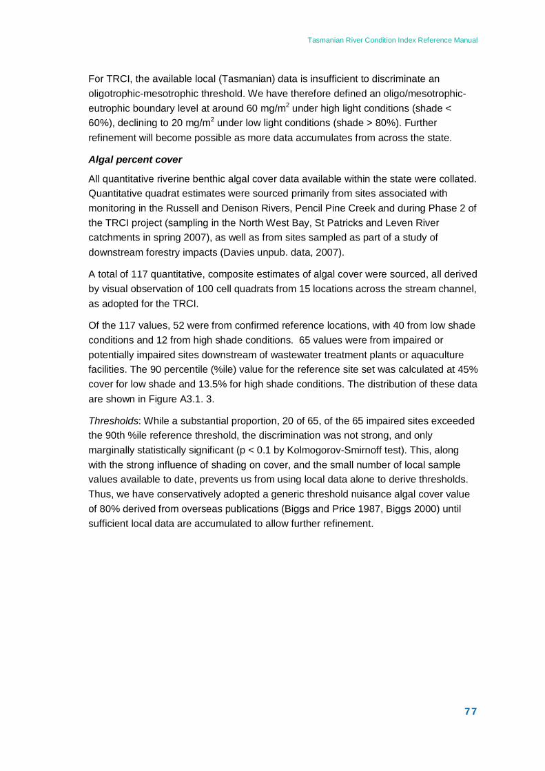
Tasmanian River Condition Index Reference Manual
77
For TRCI, the available local (Tasmanian) data is insufficient to discriminate an oligotrophic-mesotrophic threshold. We have therefore defined an oligo/mesotrophic-eutrophic boundary level at around 60 mg/m2 under high light conditions (shade < 60%), declining to 20 mg/m2 under low light conditions (shade > 80%). Further refinement will become possible as more data accumulates from across the state.
Algal percent cover
All quantitative riverine benthic algal cover data available within the state were collated. Quantitative quadrat estimates were sourced primarily from sites associated with monitoring in the Russell and Denison Rivers, Pencil Pine Creek and during Phase 2 of the TRCI project (sampling in the North West Bay, St Patricks and Leven River catchments in spring 2007), as well as from sites sampled as part of a study of downstream forestry impacts (Davies unpub. data, 2007).
A total of 117 quantitative, composite estimates of algal cover were sourced, all derived by visual observation of 100 cell quadrats from 15 locations across the stream channel, as adopted for the TRCI.
Of the 117 values, 52 were from confirmed reference locations, with 40 from low shade conditions and 12 from high shade conditions. 65 values were from impaired or potentially impaired sites downstream of wastewater treatment plants or aquaculture facilities. The 90 percentile (%ile) value for the reference site set was calculated at 45% cover for low shade and 13.5% for high shade conditions. The distribution of these data are shown in Figure A3.1. 3.
Thresholds: While a substantial proportion, 20 of 65, of the 65 impaired sites exceeded the 90th %ile reference threshold, the discrimination was not strong, and only marginally statistically significant (p < 0.1 by Kolmogorov-Smirnoff test). This, along with the strong influence of shading on cover, and the small number of local sample values available to date, prevents us from using local data alone to derive thresholds. Thus, we have conservatively adopted a generic threshold nuisance algal cover value of 80% derived from overseas publications (Biggs and Price 1987, Biggs 2000) until sufficient local data are accumulated to allow further refinement.
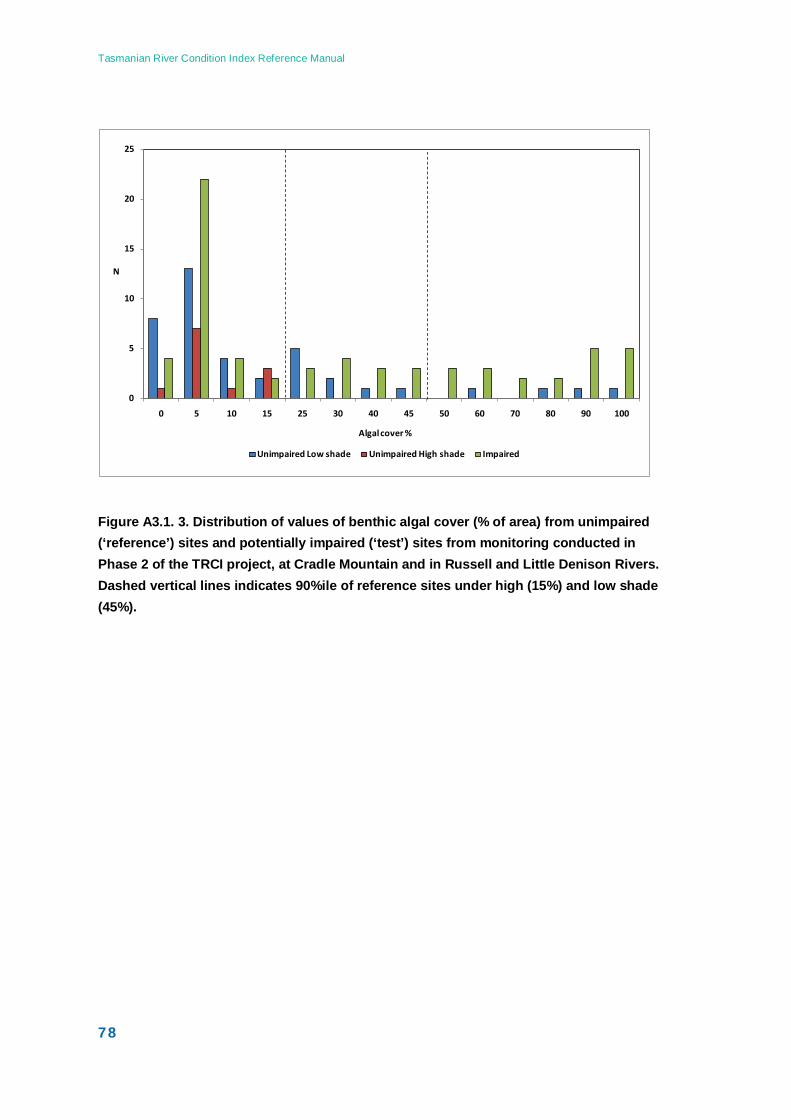
Tasmanian River Condition Index Reference Manual
78
Figure A3.1. 3. Distribution of values of benthic algal cover (% of area) from unimpaired (‘reference’) sites and potentially impaired (‘test’) sites from monitoring conducted in Phase 2 of the TRCI project, at Cradle Mountain and in Russell and Little Denison Rivers. Dashed vertical lines indicates 90%ile of reference sites under high (15%) and low shade (45%).
0
5
10
15
20
25
0 5 10 15 25 30 40 45 50 60 70 80 90 100
N
Algal cover %
Unimpaired Low shade Unimpaired High shade Impaired
Tasmanian River Condition Index Reference Manual
79
4 Hydrology Sub-Index
4.1 Introduction The objective of the hydrology sub-index is to provide an assessment of the hydrological condition of Tasmanian Rivers that can be incorporated into the overall TRCI. The assessment of ‘condition’ is based on a departure from a reference state, where reference is defined as being pre-development conditions and refers to what the flow regime would have been like without extraction, dams, or other water resource developments.
4.2 Background The flow regime is one of the key drivers of river condition, influencing the formation and maintenance of the physical habitat, ecological function and water quality. Changes to the flow regime can occur for many reasons and affect many attributes of the hydrological character of a river.
It is widely recognised that flow regulation is a major cause of deteriorating ecosystem conditions in many of Australia’s river systems (Arthington and Pusey, 2003). The ecological effects of regulation and/or extraction are generally well documented and encompass changes to riparian and aquatic plant communities (e.g. Bren, 1992; Kingsford, 2000; Mackay et al., 2001); invertebrate communities (e.g. Quinn et al, 2000), fish communities (e.g. Gehrke et al., 1995) and waterbird communities (e.g. Kingsford, 2000). It is also well recognised that changes in flow regimes cause changes to riverine geomorphology and physical habitat (e.g. Milhous, 1982; Williams and Wolman, 1984).
In Tasmania, altered land use as a result of urbanisation, agriculture and forestry activities as well as the regulation of rivers for water supply purposes and hydropower generation has changed the flow regime of many of the states rivers. The general philosophy of the TRCI of recognising the intrinsic value of all aspects of river condition (biotic and physical) resulted in a decision to use indicators of hydrological change that are relevant for aquatic biota, geomorphic processes as well as representing overall stream hydrology.
Tasmanian River Condition Index Reference Manual
80
Thus indicators were needed that would encapsulate the following features of stream hydrology:
o the change in overall volume of water carried by a waterway each year; o the change in overall flow regime; o changes in variability; o the changes in seasonality of flows, including:
• The changes in flow magnitude in ‘low flow’ and ‘high flow’ periods, and • The changes in the timing of ‘low flow’ and ‘high flow’ periods;
o changes to flooding (magnitude, duration and frequency); o changes in the number, duration and interval of ‘spells’ (periods that the flow is
above or below a threshold value); o the change in the magnitude of high flows; and o changes to overbank flows (magnitude, duration and frequency).
4.3 Component selection A range of hydrological indicators have been used in Australia to measure the hydrological condition of rivers. The major methods used in Australia have been:
o A hydrological disturbance index developed by Norris et al. (2001) for the National Land and Water Resources Audit;
o A series of indicators developed as part of the Murray-Darling Basin Commission's Sustainable Rivers Audit (SRA) (MDBC, 2004) and their non-parametric variants;
o The Flow Stress Ranking (FSR) indicators (SKM 2005) that were developed for the Victorian Index of Stream Condition (ISC). These indicators were based on the earlier work of the SRA; and
• use a non-parametric approach to account for the variability of the system
• are calculated using monthly, rather than daily flow data • have been reduced from a suite of 10 indicators to 5 statistically
independent indices.
4.3.1 Relevant flow statistics Given that all of the features of stream hydrology listed above (except for the change to overbank flows) could be represented by the FSR indicators, it was originally recommended that the FSR indicators be used (Earth Tech, 2007a; Earth Tech 2007b). However, given that the Tasmanian Hydrological models operate at a daily timestep it was considered more appropriate to test the method using the daily versions of the original 10 indicators (Earth Tech, 2007a; Earth Tech 2007b), add indicators to determine the change to overbank flow characteristics and, based on the pilot test data, determine the appropriate suite of statistically independent indices for Tasmania.

Tasmanian River Condition Index Reference Manual
81
As part of both the pilot testing and the original round of assessments in 2008, cross correlation analysis determined that there was a lack of a consistent pattern of correlation between indices across the catchments assessed, indicating that hydrological alteration in Tasmania is complex and varied between catchments. Thus, it was recommended that all 12 indicators be retained. Table 4.1 lists the final suite of indicators of hydrological changes adopted for the TRCI.
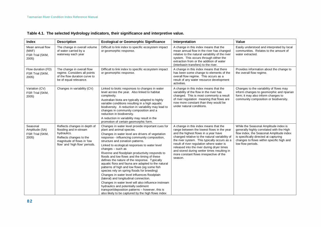
Tasmanian River Condition Index Reference Manual
82
Table 4.1. The selected Hydrology indicators, their significance and interpretive value.
Index Description Ecological or Geomorphic Significance Interpretation Value Mean annual flow (MAF) FSR Trial (SKM, 2005)
The change in overall volume of water carried by a waterway each year
Difficult to link index to specific ecosystem impact or geomorphic response.
A change in this index means that the mean annual flow in the river has changed relative to the natural variability of the river system. This occurs through either the extraction from or the addition of water (interbasin transfers) to the river.
Easily understood and interpreted by local communities. Relates to the amount of water extracted.
Flow duration (FD) FSR Trial (SKM, 2005)
The change in overall flow regime. Considers all points of the flow duration curve to be of equal relevance.
Difficult to link index to specific ecosystem impact or geomorphic response.
A change in this index means that there has been some change to elements of the overall flow regime. This occurs as a result of any water resource development activities.
Provides information about the change to the overall flow regime.
Variation (CV) FSR Trial (SKM, 2005)
Changes in variability (CV) Linked to biotic responses to changes in water level across the year. Also linked to habitat complexity. Australian biota are typically adapted to highly variable conditions resulting in a high aquatic biodiversity. A reduction in variability may lead to changes in community composition and a reduction in biodiversity. A reduction in variability may result in the promotion of certain geomorphic form.
A change in this index means that the variability of the flow in the river has changed. This is most commonly a result of river regulation meaning that flows are now more constant than they would be under natural conditions.
Changes to the variability of flows may inform changes to geomorphic and riparian form; it may also inform changes to community composition or biodiversity.
Seasonal Amplitude (SA) FSR Trial (SKM, 2005)
Reflects changes in depth of flooding and in-stream hydraulics. Reflects changes to the magnitude of flows in ‘low flow’ and ‘high flow’ periods.
Changes in water level provide important cues for plant and animal species. Changes in water level are drivers of vegetation response - influencing community composition, structure and zonation patterns. Linked to ecological responses to water level changes – such as Riverine and floodplain productivity responds to floods and low flows and the timing of these defines the nature of the response. Typically aquatic flora and fauna are adapted to the natural patterns of high and low flows (eg some fish species rely on spring floods for breeding) Changes in water level influences floodplain (lateral) and longitudinal connection. Changes in water level will also influence instream hydraulics and potentially sediment transport/deposition patterns – however, this is also likely to be captured by the high flows index
A change in this index means that the range between the lowest flows in the year and the highest flows in a year have changed relative to the natural variability of the river system. This typically occurs as a result of river regulation where water is released into the river during dryer times and stored during wetter times resulting in more constant flows irrespective of the season.
While the Seasonal Amplitude index is generally highly correlated with the High flow index, the Seasonal Amplitude index is specifically directed at capturing changes to flows within specific high and low flow periods.
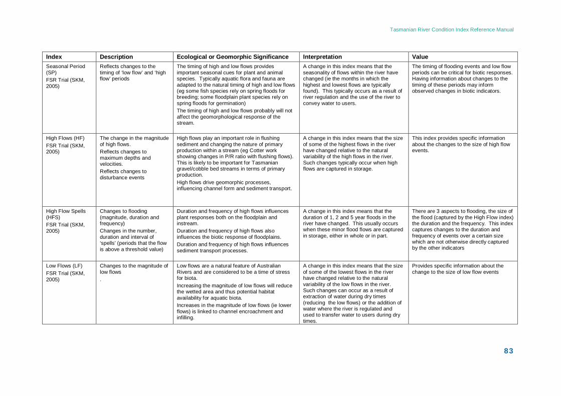
Tasmanian River Condition Index Reference Manual
83
Index Description Ecological or Geomorphic Significance Interpretation Value Seasonal Period (SP) FSR Trial (SKM, 2005)
Reflects changes to the timing of ‘low flow’ and ‘high flow’ periods
The timing of high and low flows provides important seasonal cues for plant and animal species. Typically aquatic flora and fauna are adapted to the natural timing of high and low flows (eg some fish species rely on spring floods for breeding; some floodplain plant species rely on spring floods for germination) The timing of high and low flows probably will not affect the geomorphological response of the stream.
A change in this index means that the seasonality of flows within the river have changed (ie the months in which the highest and lowest flows are typically found). This typically occurs as a result of river regulation and the use of the river to convey water to users.
The timing of flooding events and low flow periods can be critical for biotic responses. Having information about changes to the timing of these periods may inform observed changes in biotic indicators.
High Flows (HF) FSR Trial (SKM, 2005)
The change in the magnitude of high flows. Reflects changes to maximum depths and velocities. Reflects changes to disturbance events
High flows play an important role in flushing sediment and changing the nature of primary production within a stream (eg Cotter work showing changes in P/R ratio with flushing flows). This is likely to be important for Tasmanian gravel/cobble bed streams in terms of primary production. High flows drive geomorphic processes, influencing channel form and sediment transport.
A change in this index means that the size of some of the highest flows in the river have changed relative to the natural variability of the high flows in the river. Such changes typically occur when high flows are captured in storage.
This index provides specific information about the changes to the size of high flow events.
High Flow Spells (HFS) FSR Trial (SKM, 2005)
Changes to flooding (magnitude, duration and frequency) Changes in the number, duration and interval of ‘spells’ (periods that the flow is above a threshold value)
Duration and frequency of high flows influences plant responses both on the floodplain and instream. Duration and frequency of high flows also influences the biotic response of floodplains. Duration and frequency of high flows influences sediment transport processes.
A change in this index means that the duration of 1, 2 and 5 year floods in the river have changed. This usually occurs when these minor flood flows are captured in storage, either in whole or in part.
There are 3 aspects to flooding, the size of the flood (captured by the High Flow index) the duration and the frequency. This index captures changes to the duration and frequency of events over a certain size which are not otherwise directly captured by the other indicators
Low Flows (LF) FSR Trial (SKM, 2005)
Changes to the magnitude of low flows .
Low flows are a natural feature of Australian Rivers and are considered to be a time of stress for biota. Increasing the magnitude of low flows will reduce the wetted area and thus potential habitat availability for aquatic biota. Increases in the magnitude of low flows (ie lower flows) is linked to channel encroachment and infilling.
A change in this index means that the size of some of the lowest flows in the river have changed relative to the natural variability of the low flows in the river. Such changes can occur as a result of extraction of water during dry times (reducing the low flows) or the addition of water where the river is regulated and used to transfer water to users during dry times.
Provides specific information about the change to the size of low flow events
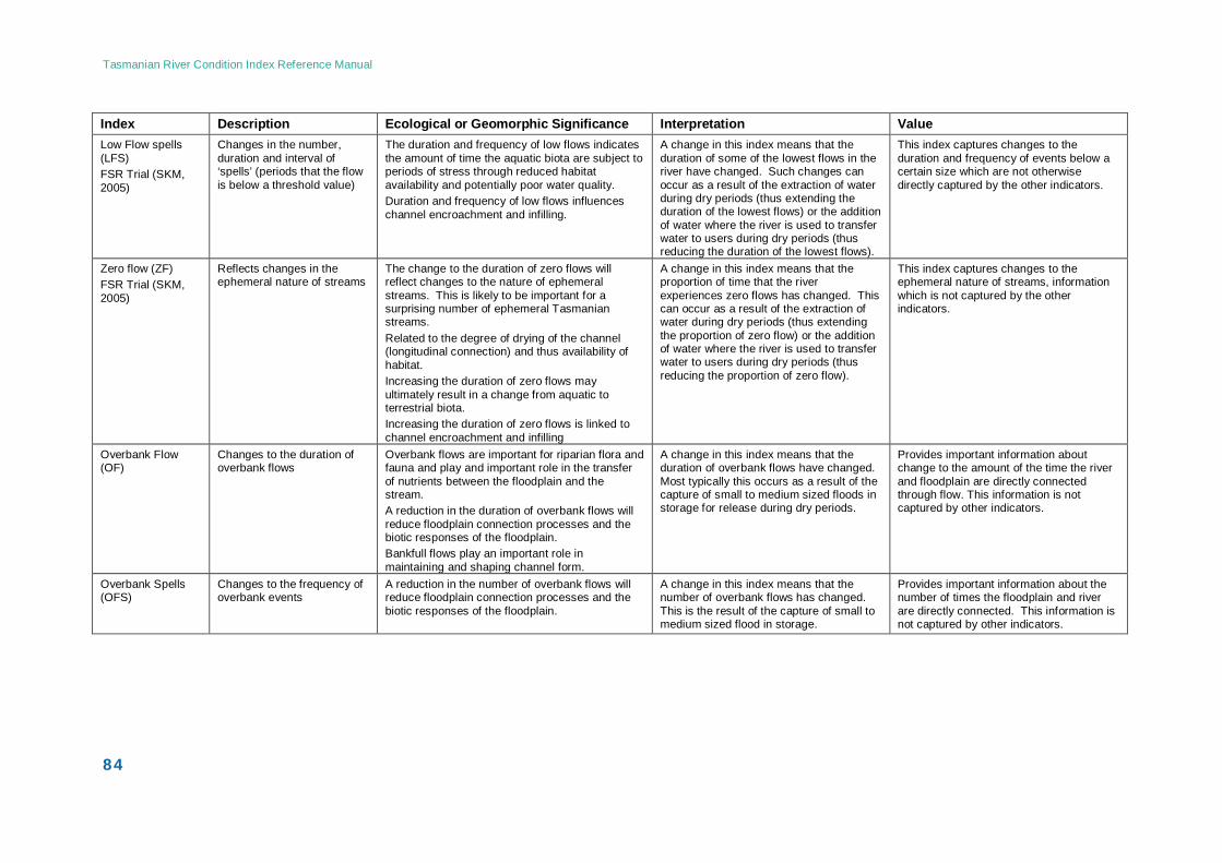
Tasmanian River Condition Index Reference Manual
84
Index Description Ecological or Geomorphic Significance Interpretation Value Low Flow spells (LFS) FSR Trial (SKM, 2005)
Changes in the number, duration and interval of ‘spells’ (periods that the flow is below a threshold value)
The duration and frequency of low flows indicates the amount of time the aquatic biota are subject to periods of stress through reduced habitat availability and potentially poor water quality. Duration and frequency of low flows influences channel encroachment and infilling.
A change in this index means that the duration of some of the lowest flows in the river have changed. Such changes can occur as a result of the extraction of water during dry periods (thus extending the duration of the lowest flows) or the addition of water where the river is used to transfer water to users during dry periods (thus reducing the duration of the lowest flows).
This index captures changes to the duration and frequency of events below a certain size which are not otherwise directly captured by the other indicators.
Zero flow (ZF) FSR Trial (SKM, 2005)
Reflects changes in the ephemeral nature of streams
The change to the duration of zero flows will reflect changes to the nature of ephemeral streams. This is likely to be important for a surprising number of ephemeral Tasmanian streams. Related to the degree of drying of the channel (longitudinal connection) and thus availability of habitat. Increasing the duration of zero flows may ultimately result in a change from aquatic to terrestrial biota. Increasing the duration of zero flows is linked to channel encroachment and infilling
A change in this index means that the proportion of time that the river experiences zero flows has changed. This can occur as a result of the extraction of water during dry periods (thus extending the proportion of zero flow) or the addition of water where the river is used to transfer water to users during dry periods (thus reducing the proportion of zero flow).
This index captures changes to the ephemeral nature of streams, information which is not captured by the other indicators.
Overbank Flow (OF)
Changes to the duration of overbank flows
Overbank flows are important for riparian flora and fauna and play and important role in the transfer of nutrients between the floodplain and the stream. A reduction in the duration of overbank flows will reduce floodplain connection processes and the biotic responses of the floodplain. Bankfull flows play an important role in maintaining and shaping channel form.
A change in this index means that the duration of overbank flows have changed. Most typically this occurs as a result of the capture of small to medium sized floods in storage for release during dry periods.
Provides important information about change to the amount of the time the river and floodplain are directly connected through flow. This information is not captured by other indicators.
Overbank Spells (OFS)
Changes to the frequency of overbank events
A reduction in the number of overbank flows will reduce floodplain connection processes and the biotic responses of the floodplain.
A change in this index means that the number of overbank flows has changed. This is the result of the capture of small to medium sized flood in storage.
Provides important information about the number of times the floodplain and river are directly connected. This information is not captured by other indicators.
Tasmanian River Condition Index Reference Manual
85
4.4 Hydrological data Flow records from a river (termed ‘observations’) display the combined effects of climatic variation, changes in water resource development and changes in land use. Separating the effects of each from within a flow record is almost impossible (e.g. is the reduction in flow observed in a river a consequence of a change in climate, a change in demand, or a combination of both) and comparing flow data from different time periods leads to spurious assessments of condition because of the effect of different climate periods.
To address this problem, models have been developed that create a long term flow record based on a defined set of conditions. These models are based on climatic data (rainfall-runoff models), and different river management scenarios (e.g. regulation, extraction, landcover) are incorporated within them. Thus, assessments of hydrological change typically use paired modelled data sets such as:
1. a long term flow record that represents the flow in the river under ‘reference’ or natural conditions (no extractions, no regulation and a natural landcover), and
2. a long term flow record that represents the flow in the river under a particular management scenario (eg, applying a specific extraction to the entire period of record).
Comparison is then made between the flows that would occur under current management regimes and those that occur under “reference” conditions. Because both modelled data sets have the same climate signal, the comparison can effectively determine the consequences of management regimes.
The use of modelled data pairs means that the changes that occur as a result of management actions can be detected, and even predicted, provided the models are capable of incorporating the specific management changes. The change typically measured is that which results from river regulation and/or substantial flow diversion or extraction. It is considerably more difficult to include the flow regime changes resulting from land use change and/or groundwater use into the models and this is an area for continued development.
The Department of Primary Industries and Water has developed surface water models (at a daily timestep) for a large proportion of Tasmania’s rural catchments. The remaining catchments exist within Tasmania’s World Heritage Area, in catchments with negligible allocation or catchments where water is solely used for hydro electricity generation. Some private models exist for those catchments in which hydro-electricity generation occurs. Tasmania is very fortunate to have such good modelling coverage.
Within a catchment, modelled hydrological data is generated for a series of points on the river network termed ‘nodes’. These nodes usually represent a point at which the
Tasmanian River Condition Index Reference Manual
86
flow in the river changes – either through the input of a major tributary or the manipulation of the flow (eg. a weir or extraction point).
4.5 Defining reference condition The current surface water modelling (by DPIW) in Tasmania defines reference condition (natural flows) as being no water resource development (no dams or extractions). The models do not specifically take into account land-use changes (clearing or re-forestation). Groundwater use is incorporated into a small proportion of the state’s models.
As datasets become available which account for groundwater use and landuse change, DPIW may incorporate these into their models. The latest models should be used for the application of the TRCI. Modelled data are available from the relevant DPIW Branch ([email protected]).
4.6 Description of components The Hydrology sub-index comprises 12 component indices calculated from modelled time series data. The 12 indices provide insight into the changes to different aspects of the flow regime that have occurred as a result of water resource development (refer to Table 4.1). The 12 component indices are:
1. Mean Annual Flow Index (MAF)
2. Flow Duration index (FD)
3. Variation Index (CV)
4. Seasonal Amplitude Index (SA)
5. Seasonal Period Index (SP)
6. High Flow Index (HF)
7. High Flow Spells Index (HFS)
8. Low Flow Index (LF)
9. Low Flow Spells Index (LFS)
10. Proportion of Zero Flows Index (PZ)
11. Overbank Flows Index (OF)
12. Overbank Spells Index (OFS)
The index calculations are a relatively complex set of mathematical processes that are not easily understood by those without a background in Hydrology or mathematics.
Tasmanian River Condition Index Reference Manual
87
This is because the calculations are set up to account for the natural variability in the flow regime and determine if the ‘current’ flow conditions fall within the range of natural flow conditions in the river. Such an approach is adopted because it is thought to increase the ecological relevance of the assessment. For example, it is assumed that extracting 20% of the water from a river is likely to have fewer adverse effects on the aquatic biota of a river that is naturally highly variable in flows, than a river that has consistent flows. The descriptions in Table 4.1 provide sufficient information about the indices for most users of the TRCI but, for completeness, a detailed description is also provided below (these descriptions are modified from those contained in SKM, 2005). The non-Hydrologist is referred to the comprehensive glossary of terms at the beginning of this report to assist in understanding the following descriptions.
Each component hydrology index produces a score between 0 and 1. The following standard terminology is used to describe the degree of change from natural (unimpacted) condition:
o Largely unmodified – score of 0.8 or greater o Slightly modified – score from 0.6 to < 0.8 o Moderately modified – score from 0.4 to < 0.6 o Substantially modified – score from 0.2 to < 0.4 o Severely modified – score < 0.2
4.6.1 Mean Annual Flow Index (MAF) The mean annual flow index (MAF) is based around the difference between the percentage of time that the unimpacted and current mean annual flows are exceeded under unimpacted conditions. The advantage of using a range-standardised index is that it takes into account whether the current conditions fall within the unimpacted flow regime. This method of calculating the range standardised index also has the advantage of using the actual distribution of the unimpacted annual flows, rather than assuming that the mean annual flows are normally distributed. The formulation of a range-standardised index for mean annual flow is given by
( ) ( )cileuilem QPQPA −×−= 21 (1)
Where: Am = Range-standardised mean annual flow index
Qc = Average current annual flow (ML/year)
Qu = Average unimpacted annual flow (ML/year)
Pile(Qc) = Proportion of years that the average current annual flow is exceeded under unimpacted conditions
Pile(Qu) = Proportion of years that the average unimpacted annual flow is exceeded under unimpacted conditions
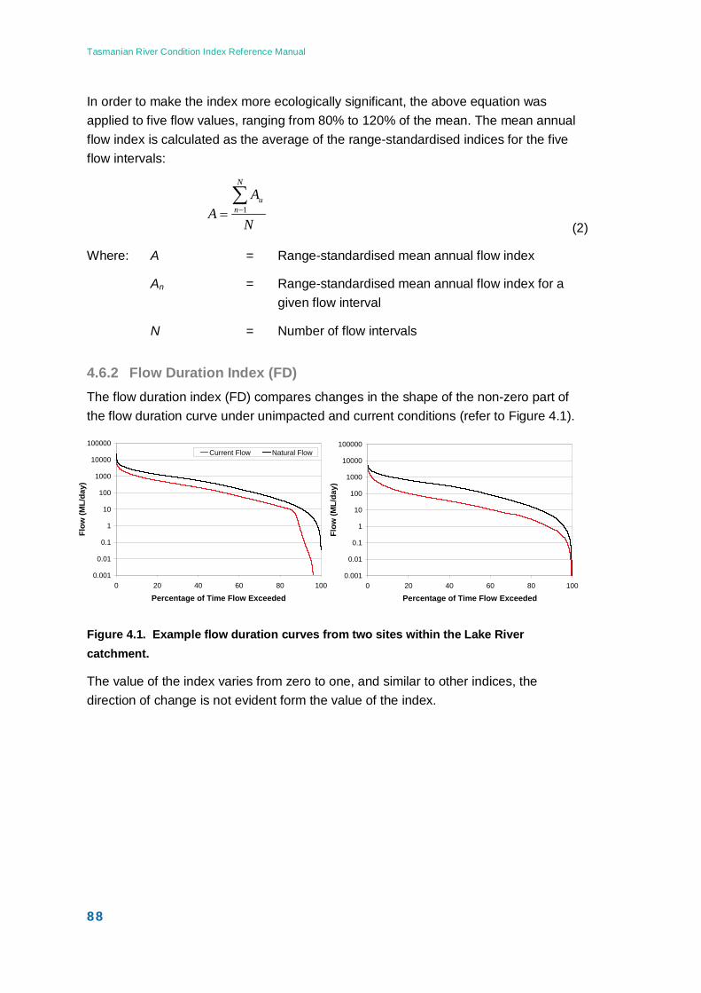
Tasmanian River Condition Index Reference Manual
88
In order to make the index more ecologically significant, the above equation was applied to five flow values, ranging from 80% to 120% of the mean. The mean annual flow index is calculated as the average of the range-standardised indices for the five flow intervals:
N
AA
N
nu∑
−= 1
(2)
Where: A = Range-standardised mean annual flow index
An = Range-standardised mean annual flow index for a given flow interval
N = Number of flow intervals
4.6.2 Flow Duration Index (FD) The flow duration index (FD) compares changes in the shape of the non-zero part of the flow duration curve under unimpacted and current conditions (refer to Figure 4.1).
0.001
0.01
0.1
1
10
100
1000
10000
100000
0 20 40 60 80 100
Percentage of Time Flow Exceeded
Flow
(ML/
day)
Current Flow Natural Flow
0.001
0.01
0.1
1
10
100
1000
10000
100000
0 20 40 60 80 100
Percentage of Time Flow Exceeded
Flow
(ML/
day)
Figure 4.1. Example flow duration curves from two sites within the Lake River catchment.
The value of the index varies from zero to one, and similar to other indices, the direction of change is not evident form the value of the index.
Tasmanian River Condition Index Reference Manual
89
If the flow duration curve is unchanged between unimpacted and current conditions, then the value of the index is 1.
( ) ( ){ }( ) ( ){ }
=
cileuile
cileuile
QPQPQPQPmeanFD
,max,min
(3)
Where: FD = Flow duration index
Qn = flow under unimpacted conditions (at equal log intervals)
Pile(Qu) = the proportion of time that the flow Qn is exceeded under unimpacted conditions
Qc = the flow under current conditions that has an exceedance percentile equal to Pile(Qu)
Pile(Qc) = the proportion of time that the flow Qc is exceeded under unimpacted conditions
4.6.3 Variation index (CV) The variation index compares the coefficient of variation of daily flows between current and unimpacted conditions. This index was slightly modified from that used in the SRA to ensure that the index varies from zero to one, where a value of one indicates no change to the coefficient of variation. The index is calculated as the ratio of the daily flows under unimpacted and current conditions, where the coefficient of variation is defined as the standard deviation divided by the mean.
( )( )cu
cu
CVCVCVCVCV,max,min
= (4)
Where: CV = Index of daily variability
CVc = Current daily coefficient of variation
CVu = Unimpacted daily coefficient of variation
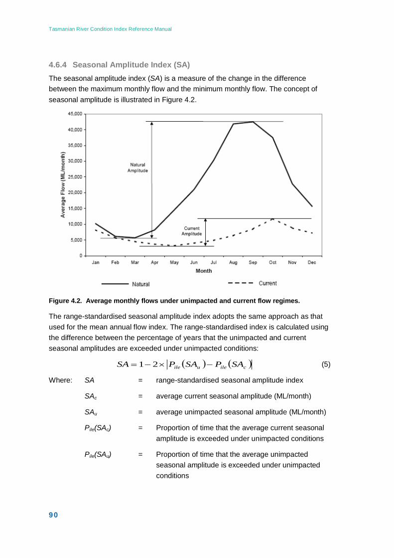
Tasmanian River Condition Index Reference Manual
90
4.6.4 Seasonal Amplitude Index (SA) The seasonal amplitude index (SA) is a measure of the change in the difference between the maximum monthly flow and the minimum monthly flow. The concept of seasonal amplitude is illustrated in Figure 4.2.
Figure 4.2. Average monthly flows under unimpacted and current flow regimes.
The range-standardised seasonal amplitude index adopts the same approach as that used for the mean annual flow index. The range-standardised index is calculated using the difference between the percentage of years that the unimpacted and current seasonal amplitudes are exceeded under unimpacted conditions:
( ) ( )cileuile SAPSAPSA −×−= 21 (5)
Where: SA = range-standardised seasonal amplitude index
SAc = average current seasonal amplitude (ML/month)
SAu = average unimpacted seasonal amplitude (ML/month)
Pile(SAc) = Proportion of time that the average current seasonal amplitude is exceeded under unimpacted conditions
Pile(SAu) = Proportion of time that the average unimpacted seasonal amplitude is exceeded under unimpacted conditions
Tasmanian River Condition Index Reference Manual
91
The average seasonal amplitude is computed as the arithmetic average of the time series of the difference between minimum and maximum monthly flows in each calendar year.
4.6.5 Seasonal period index (SP) The index compares the unimpacted and current frequency distribution of maximum and minimum monthly flows. The first step in calculating the index is to create frequency distributions that show the percentage of years that peak and minimum annual flows fall within each given month under current and unimpacted conditions. The index is then calculated by summing the minimum proportions (from unimpacted or current) within each month. In MDBC (2003) the index is presented in terms of the number of years the peak or minimum flow falls within each given month. In this report the percentage of years the peak or minimum flow falls within each given month has been used. The equation used is presented below.
( )[ ] ( )[ ]
+= ∑∑== 11
;;2001_
iii
iii PLUPLCMINPHUPHCMINfdSP (6)
Where: SP_fd = Comparison of frequency distribution seasonal period index
PHCi = The percentage of years the ith month has the peak annual flow under current conditions (%).
PHUi = The percentage of years the ith month has the peak annual flow under unimpacted conditions (%).
PLCi = The percentage of years the ith month has the minimum annual flow under current conditions (%).
PLUi = The percentage of years the ith month has the minimum annual flow under unimpacted conditions (%).
4.6.6 High flow index (HF) The high flow index is a measure of the change in high flow magnitude from unimpacted to current conditions. The approach adopted to calculate the high flow index is similar to that used to calculate the low flow index. The monthly high flow index is calculated based on the 10 % and 20 % exceedance flows.
The index is calculated using the difference between the percentage of years that the unimpacted and current 10 % exceedance flows (evaluated over the whole period of record) are exceeded by the annual 10 percentile flow (evaluated on a year-by-year
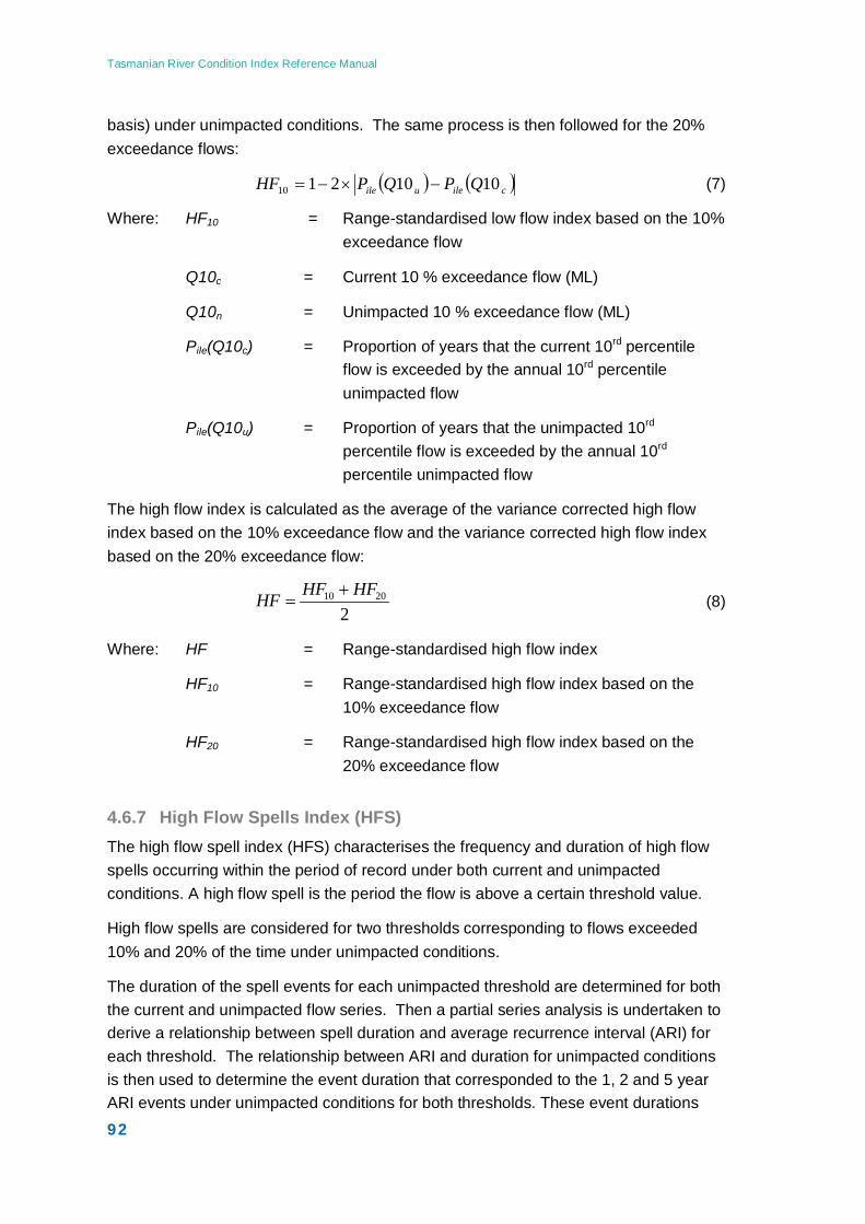
Tasmanian River Condition Index Reference Manual
92
basis) under unimpacted conditions. The same process is then followed for the 20% exceedance flows:
( ) ( )cileuile QPQPHF 10102110 −×−= (7)
Where: HF10 = Range-standardised low flow index based on the 10% exceedance flow
Q10c = Current 10 % exceedance flow (ML)
Q10n = Unimpacted 10 % exceedance flow (ML)
Pile(Q10c) = Proportion of years that the current 10rd percentile flow is exceeded by the annual 10rd percentile unimpacted flow
Pile(Q10u) = Proportion of years that the unimpacted 10rd percentile flow is exceeded by the annual 10rd percentile unimpacted flow
The high flow index is calculated as the average of the variance corrected high flow index based on the 10% exceedance flow and the variance corrected high flow index based on the 20% exceedance flow:
22010 HFHFHF +
= (8)
Where: HF = Range-standardised high flow index
HF10 = Range-standardised high flow index based on the 10% exceedance flow
HF20 = Range-standardised high flow index based on the 20% exceedance flow
4.6.7 High Flow Spells Index (HFS) The high flow spell index (HFS) characterises the frequency and duration of high flow spells occurring within the period of record under both current and unimpacted conditions. A high flow spell is the period the flow is above a certain threshold value.
High flow spells are considered for two thresholds corresponding to flows exceeded 10% and 20% of the time under unimpacted conditions.
The duration of the spell events for each unimpacted threshold are determined for both the current and unimpacted flow series. Then a partial series analysis is undertaken to derive a relationship between spell duration and average recurrence interval (ARI) for each threshold. The relationship between ARI and duration for unimpacted conditions is then used to determine the event duration that corresponded to the 1, 2 and 5 year ARI events under unimpacted conditions for both thresholds. These event durations
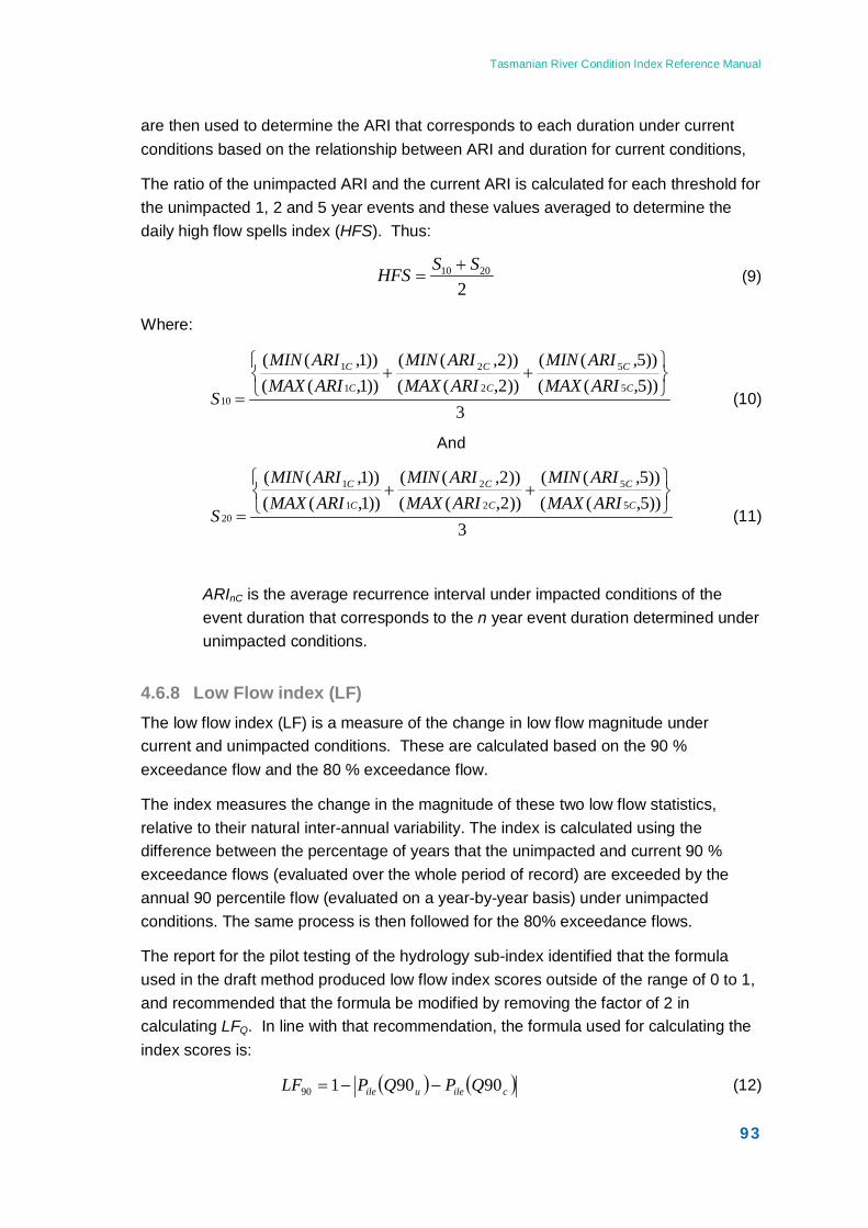
Tasmanian River Condition Index Reference Manual
93
are then used to determine the ARI that corresponds to each duration under current conditions based on the relationship between ARI and duration for current conditions,
The ratio of the unimpacted ARI and the current ARI is calculated for each threshold for the unimpacted 1, 2 and 5 year events and these values averaged to determine the daily high flow spells index (HFS). Thus:
22010 SSHFS +
= (9)
Where:
3))5,(())5,((
))2,(())2,((
))1,(())1,((
5
5
2
2
1
1
10
++=
C
C
C
C
C
C
ARIMAXARIMIN
ARIMAXARIMIN
ARIMAXARIMIN
S (10)
And
3))5,(())5,((
))2,(())2,((
))1,(())1,((
5
5
2
2
1
1
20
++=
C
C
C
C
C
C
ARIMAXARIMIN
ARIMAXARIMIN
ARIMAXARIMIN
S (11)
ARInC is the average recurrence interval under impacted conditions of the event duration that corresponds to the n year event duration determined under unimpacted conditions.
4.6.8 Low Flow index (LF) The low flow index (LF) is a measure of the change in low flow magnitude under current and unimpacted conditions. These are calculated based on the 90 % exceedance flow and the 80 % exceedance flow.
The index measures the change in the magnitude of these two low flow statistics, relative to their natural inter-annual variability. The index is calculated using the difference between the percentage of years that the unimpacted and current 90 % exceedance flows (evaluated over the whole period of record) are exceeded by the annual 90 percentile flow (evaluated on a year-by-year basis) under unimpacted conditions. The same process is then followed for the 80% exceedance flows.
The report for the pilot testing of the hydrology sub-index identified that the formula used in the draft method produced low flow index scores outside of the range of 0 to 1, and recommended that the formula be modified by removing the factor of 2 in calculating LFQ. In line with that recommendation, the formula used for calculating the index scores is:
( ) ( )cileuile QPQPLF 9090190 −−= (12)
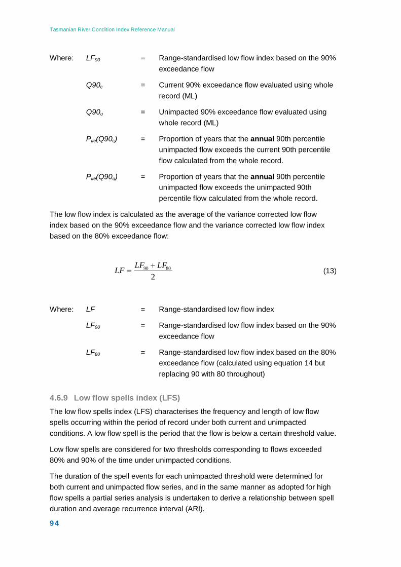
Tasmanian River Condition Index Reference Manual
94
Where: LF90 = Range-standardised low flow index based on the 90% exceedance flow
Q90c = Current 90% exceedance flow evaluated using whole record (ML)
Q90u = Unimpacted 90% exceedance flow evaluated using whole record (ML)
Pile(Q90c) = Proportion of years that the annual 90th percentile unimpacted flow exceeds the current 90th percentile flow calculated from the whole record.
Pile(Q90u) = Proportion of years that the annual 90th percentile unimpacted flow exceeds the unimpacted 90th percentile flow calculated from the whole record.
The low flow index is calculated as the average of the variance corrected low flow index based on the 90% exceedance flow and the variance corrected low flow index based on the 80% exceedance flow:
28090 LFLFLF +
= (13)
Where: LF = Range-standardised low flow index
LF90 = Range-standardised low flow index based on the 90% exceedance flow
LF80 = Range-standardised low flow index based on the 80% exceedance flow (calculated using equation 14 but replacing 90 with 80 throughout)
4.6.9 Low flow spells index (LFS) The low flow spells index (LFS) characterises the frequency and length of low flow spells occurring within the period of record under both current and unimpacted conditions. A low flow spell is the period that the flow is below a certain threshold value.
Low flow spells are considered for two thresholds corresponding to flows exceeded 80% and 90% of the time under unimpacted conditions.
The duration of the spell events for each unimpacted threshold were determined for both current and unimpacted flow series, and in the same manner as adopted for high flow spells a partial series analysis is undertaken to derive a relationship between spell duration and average recurrence interval (ARI).
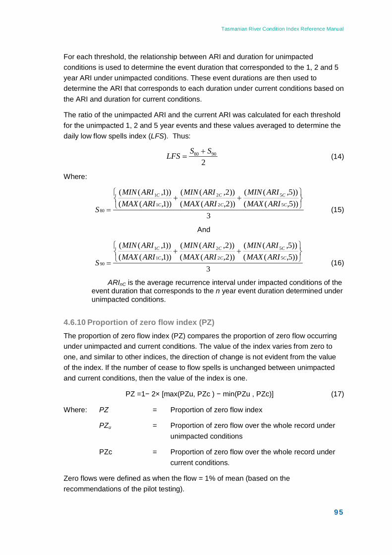
Tasmanian River Condition Index Reference Manual
95
For each threshold, the relationship between ARI and duration for unimpacted conditions is used to determine the event duration that corresponded to the 1, 2 and 5 year ARI under unimpacted conditions. These event durations are then used to determine the ARI that corresponds to each duration under current conditions based on the ARI and duration for current conditions.
The ratio of the unimpacted ARI and the current ARI was calculated for each threshold for the unimpacted 1, 2 and 5 year events and these values averaged to determine the daily low flow spells index (LFS). Thus:
29080 SSLFS +
= (14)
Where:
3))5,(())5,((
))2,(())2,((
))1,(())1,((
5
5
2
2
1
1
80
++=
C
C
C
C
C
C
ARIMAXARIMIN
ARIMAXARIMIN
ARIMAXARIMIN
S (15)
And
3))5,(())5,((
))2,(())2,((
))1,(())1,((
5
5
2
2
1
1
90
++=
C
C
C
C
C
C
ARIMAXARIMIN
ARIMAXARIMIN
ARIMAXARIMIN
S (16)
ARInC is the average recurrence interval under impacted conditions of the event duration that corresponds to the n year event duration determined under unimpacted conditions.
4.6.10 Proportion of zero flow index (PZ) The proportion of zero flow index (PZ) compares the proportion of zero flow occurring under unimpacted and current conditions. The value of the index varies from zero to one, and similar to other indices, the direction of change is not evident from the value of the index. If the number of cease to flow spells is unchanged between unimpacted and current conditions, then the value of the index is one.
PZ =1− 2× [max(PZu, PZc ) − min(PZu , PZc)] (17)
Where: PZ = Proportion of zero flow index
PZu = Proportion of zero flow over the whole record under unimpacted conditions
PZc = Proportion of zero flow over the whole record under current conditions.
Zero flows were defined as when the flow = 1% of mean (based on the recommendations of the pilot testing).
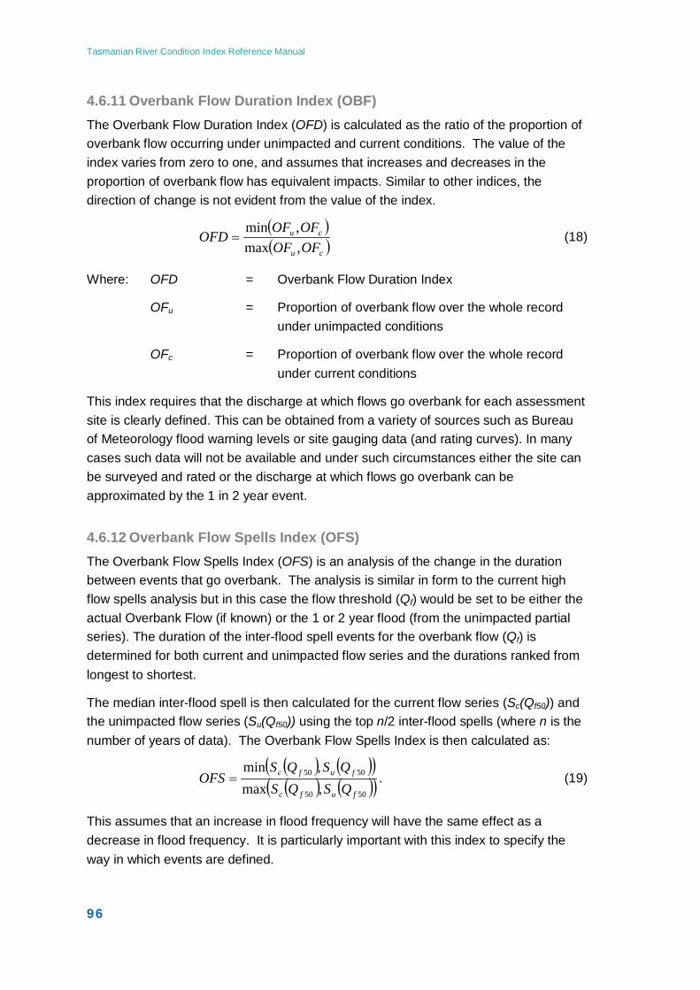
Tasmanian River Condition Index Reference Manual
96
4.6.11 Overbank Flow Duration Index (OBF) The Overbank Flow Duration Index (OFD) is calculated as the ratio of the proportion of overbank flow occurring under unimpacted and current conditions. The value of the index varies from zero to one, and assumes that increases and decreases in the proportion of overbank flow has equivalent impacts. Similar to other indices, the direction of change is not evident from the value of the index.
( )( )cu
cu
OFOFOFOF
OFD,max,min
= (18)
Where: OFD = Overbank Flow Duration Index
OFu = Proportion of overbank flow over the whole record under unimpacted conditions
OFc = Proportion of overbank flow over the whole record under current conditions
This index requires that the discharge at which flows go overbank for each assessment site is clearly defined. This can be obtained from a variety of sources such as Bureau of Meteorology flood warning levels or site gauging data (and rating curves). In many cases such data will not be available and under such circumstances either the site can be surveyed and rated or the discharge at which flows go overbank can be approximated by the 1 in 2 year event.
4.6.12 Overbank Flow Spells Index (OFS) The Overbank Flow Spells Index (OFS) is an analysis of the change in the duration between events that go overbank. The analysis is similar in form to the current high flow spells analysis but in this case the flow threshold (Qf) would be set to be either the actual Overbank Flow (if known) or the 1 or 2 year flood (from the unimpacted partial series). The duration of the inter-flood spell events for the overbank flow (Qf) is determined for both current and unimpacted flow series and the durations ranked from longest to shortest.
The median inter-flood spell is then calculated for the current flow series (Sc(Qf50)) and the unimpacted flow series (Su(Qf50)) using the top n/2 inter-flood spells (where n is the number of years of data). The Overbank Flow Spells Index is then calculated as:
( ) ( )( )( ) ( )( )5050
5050
,max,min
fufc
fufc
QSQSQSQS
OFS = . (19)
This assumes that an increase in flood frequency will have the same effect as a decrease in flood frequency. It is particularly important with this index to specify the way in which events are defined.
Tasmanian River Condition Index Reference Manual
97
4.7 Resources required The Hydrology sub-index is calculated at the desktop using modelled flow data and as such an up to date computer is required to enable processing of the data. Two “programs” have been developed to partially automate the calculation of the index values. These are available from NRM South.
4.7.1 Training It is possible to conduct the Hydrology assessments using only the TRCI Users Manual and good computer literacy. However, it will be beneficial to have a good understanding of stream hydrology and the types of water resource development occurring within the region of interest.
4.7.2 Data requirements The calculation of the component Hydrology Indices uses modelled time series data at a daily timestep. These data are modelled for current water resource development conditions (typically specified as a year) and natural conditions (pre-development conditions). These data can be obtained from the DPIW Water Assessment branch or from Hydro-Tasmania depending on the assessment area.
It is important to note that the DPIW Hydrological models have been developed for water resource management purposes and the calibration of the models is typically best at high flows. The DPIW Water Assessment branch will need to be contacted for the provision of data prior to undertaking assessments and it is recommended that the specific purpose of the assessments be discussed with the branch at this time to determine if the models and their calibrations are appropriate.
It is recommended that between 30 and 50 years of modelled hydrological data (current and natural) is used to calculate the indices, however, it is possible to calculate reliable estimates of the component indices using a minimum of 15 years of modelled hydrological data. It is important to note that the greater the period of record, the greater the confidence in the calculated indices.
4.8 Scoring - Hydrology score at a node The Hydrology sub-index score at a data node is calculated by taking the average of all component scores.
4.9 Scoring – Hydrology score for a reporting unit The Hydrology Score for a given reporting unit is determined as the weighted median of the individual hydrology scores, where they are weighted by the length of stream represented by the point. Modelled Hydrology data will typically be available for a
Tasmanian River Condition Index Reference Manual
98
series of standard nodes (points) within the stream network sampled. These points will represent differing lengths of stream (refer to the Users’ manual for the procedures to use to calculate this).
4.9.1 Determining the length of stream represented by the sdata from a node
Within a stream network, flow statistics from a point (node) will represent a length of stream extending above and below the point until there are significant changes to the flow, for example the addition of a tributary stream of equal order or the presence of an impoundment.
To determine the length of stream represented by the data requires either manual analysis of the stream network or coding within GIS following the rules set out below (with an example from a stream network in Figure 4.3) for determining the upstream and downstream extents.
4.9.1.1 Upstream extent
Follow the trunk stream upstream until either:
a. the confluence of a tributary of one stream order less than the trunk stream; or
b. a regulating structure (such as a weir or impoundment or known major extraction point).
If another data point is reached before a confluence or regulating structure, the upstream extent shall be deemed to be halfway between the two data points.
4.9.1.2 Downstream extent
Follow the trunk stream downstream until either:
a. the confluence of a tributary of the same order as the trunk stream; or
b. a regulating structure (such as a weir or impoundment or known major extraction point).
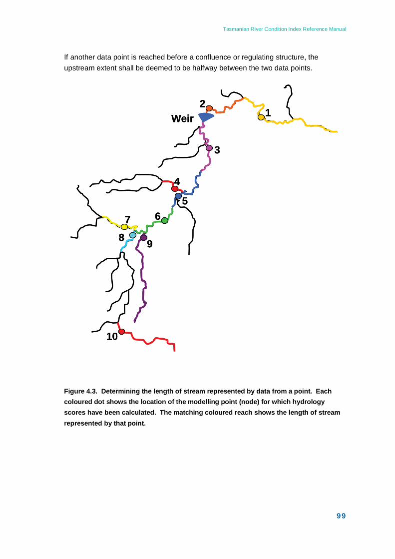
Tasmanian River Condition Index Reference Manual
99
If another data point is reached before a confluence or regulating structure, the upstream extent shall be deemed to be halfway between the two data points.
Figure 4.3. Determining the length of stream represented by data from a point. Each coloured dot shows the location of the modelling point (node) for which hydrology scores have been calculated. The matching coloured reach shows the length of stream represented by that point.
12
3
4
567
8 9
10
Weir 12
3
4
567
8 9
10
Weir
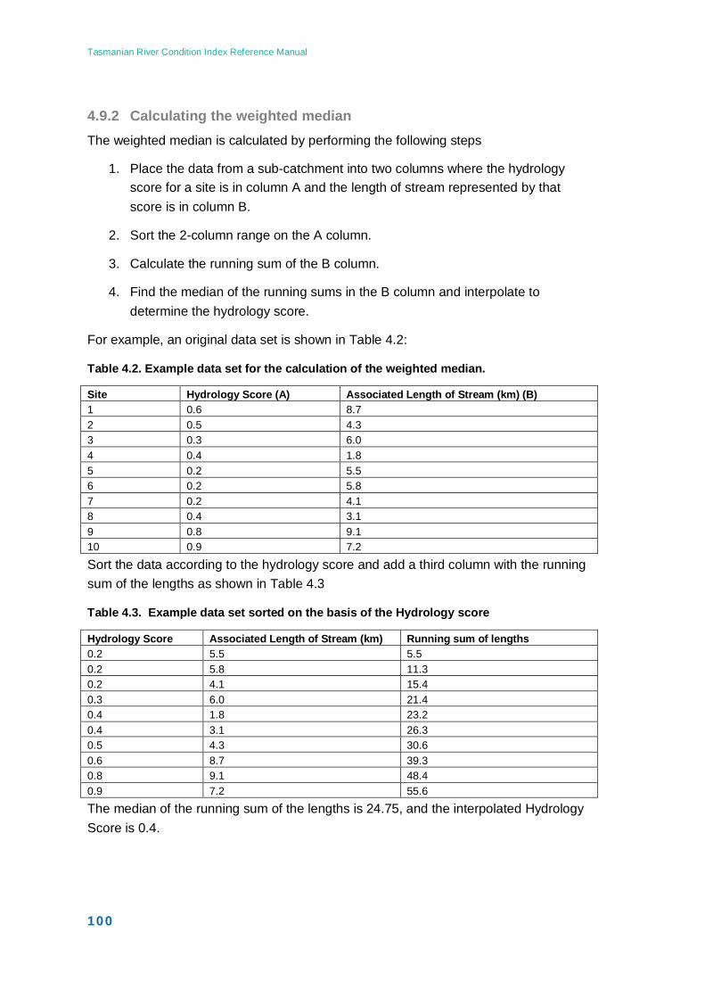
Tasmanian River Condition Index Reference Manual
100
4.9.2 Calculating the weighted median The weighted median is calculated by performing the following steps
1. Place the data from a sub-catchment into two columns where the hydrology score for a site is in column A and the length of stream represented by that score is in column B.
2. Sort the 2-column range on the A column.
3. Calculate the running sum of the B column.
4. Find the median of the running sums in the B column and interpolate to determine the hydrology score.
For example, an original data set is shown in Table 4.2:
Table 4.2. Example data set for the calculation of the weighted median.
Site Hydrology Score (A) Associated Length of Stream (km) (B) 1 0.6 8.7 2 0.5 4.3 3 0.3 6.0 4 0.4 1.8 5 0.2 5.5 6 0.2 5.8 7 0.2 4.1 8 0.4 3.1 9 0.8 9.1 10 0.9 7.2
Sort the data according to the hydrology score and add a third column with the running sum of the lengths as shown in Table 4.3
Table 4.3. Example data set sorted on the basis of the Hydrology score
Hydrology Score Associated Length of Stream (km) Running sum of lengths 0.2 5.5 5.5 0.2 5.8 11.3 0.2 4.1 15.4 0.3 6.0 21.4 0.4 1.8 23.2 0.4 3.1 26.3 0.5 4.3 30.6 0.6 8.7 39.3 0.8 9.1 48.4 0.9 7.2 55.6
The median of the running sum of the lengths is 24.75, and the interpolated Hydrology Score is 0.4.
Tasmanian River Condition Index Reference Manual
101
4.10 Missing data Given that the hydrology indicators are calculated using modelled data pairs, all of the component indicators are calculated at once and missing data to calculate an individual component will not be an issue.
Hydrology scores for catchments are typically calculated using modelled data from a set of standard modelling nodes defined by DPIW. However, there may be situations in which assessments are required at particular sites of interest. If this occurs it is entirely possibly, depending on the extent of modelling within catchments, data may be missing for the particular sites of interest. It is most likely that data will be available for nodes on trunk streams and major tributaries but not for smaller tributaries. It may also be possible that the spacing of modelling nodes means that data are missing for sites of interest between nodes.
There are two ways of providing statistics for points between model nodes:
1. interpolate the flow statistics themselves using linear interpolation (by catchment area);
2. interpolate the data used to produce the statistics.
The most robust method of doing this is to interpolate the data used to produce the statistics, effectively creating a new model node. This is not a trivial exercise and it is recommended that discussions are held with DPIW modellers prior to requesting data from specific locations.
4.10.1 Limitations of the method The DPIW hydrology models have been calibrated to provide accurate estimates of yield and therefore provide less reliable estimates of low flows and large floods. This means that the uncertainty associated with the indicators relating to low flows is higher than for other indicators. This affects the Low Flow (LF), Low Flow Spells (LFS), and Zero Flow (ZF) indices.
4.11 References - Hydrology Arthington, A.H. and Pusey, B.J. (2003) Flow Restoration and Protection in Australian Rivers. River Research and Applications. 19:377-395.
Bren, L.J. (1992) Tree invasion of an intermittent wetland in relation to changes in the flooding frequency of the River Murray, Australia. Australian Journal of Ecology 17: 395-408.
Earth Tech (2007a) River Condition Index (RCI) Framework for Tasmania: Recommended Approach. A report to NRM South. Earth Tech. Wangaratta, Victoria.
Tasmanian River Condition Index Reference Manual
102
Earth Tech (2007b) River Condition Index (RCI) Framework for Tasmania: Draft Method for Testing. A report to NRM South. Earth Tech. Wangaratta, Victoria.
Gehrke P.C., Brown, P., Schiller, C.B., Moffatt, D.B., Bruce, A.M. (1995) River Regulation and fish communities in the Murray-Darling River system, Australia. Regulated Rivers: Research and Management 11: 363-375.
Kingsford, R.T. (2000) Ecological impacts of dams, water diversions and river management on floodplain wetlands in Australia. Austral Ecology 25: 109-127.
Mackay S.J., Arthington, A.H., Werren, G., (2001) Ecological impact of weris in the Pioneer Catchment, Queensland. In The Way Forward on Weirs, Blanch S (ed.). Inland Rivers Network: Sydney; 39-58.
Milhous, R.T., (1982) Effect of Sediment Transport and Flow Regulation on the Ecology of Gravel-bed Rivers. Gravel-Bed Rivers: Fluvial Processes, Engineering and Management, R.D. Hey, J.C. Bathurst, and C.R. Thorne Ed., Wiley, New York pp 819-842.
Norris R.H., Prosser I., Young B., Liston P., Bauer N., Davies N., Dyer F., Linke S. & Thoms M. (2001) The Assessment of River Condition (ARC). An audit of the ecological condition of Australian Rivers. Final report submitted to the National Land and Water Resources Audit Office, Canberra, Australia.
Quinn G.P., Hillman, T.J., Cook, R. (2000) The response of macroinvertebrates to inundation in floodplain wetlands: a possible effect of river regulation? Regulated Rivers: Research and Management 16: 469-477.
http://audit.ea.gov.au/ANRA/water/docs/river_assessment/River_assessment.pdf
SKM, (2005) Development and Application of a Flow Stressed Ranking Procedure. A report to the Department of Sustainability and Environment. Victoria.
Williams, G.P. and Wolman, M.G. (1984) Downstream effects of dams on alluvial rivers. US Geological Survey Professional paper 1286, Washington, D.C..
Tasmanian River Condition Index Reference Manual
103
5 Physical Form Sub-Index
5.1 Introduction The objective of the Physical Form sub-index is to provide an assessment of the geomorphological condition of Tasmanian Rivers. The assessment of ‘condition’ is based on departure from reference (expected) condition. Reference condition is defined as pre-European condition.
A new approach to geomorphological condition assessment has been developed for the TRCI, as existing methods were not appropriate and reference conditions were not readily available (Section 5.2).
In order to score condition, stream reaches are classified into TRCI River Types (river types). Geomorphic benchmarks (benchmarks) have been developed which describe the pre-European character of each river type.
Scores are calculated for assessment sites by comparing site data with the expected conditions listed in the appropriate benchmark. The Physical Form sub-index includes 13 components, four of which are assessed at the desktop and nine are assessed in the field. While the raw data for all components are recorded at each site, only the relevant components are scored in particular river types.
The creation of this new method, including the development and documentation of geomorphic benchmarks, has demanded significant resources, and the method has not been as comprehensively tested as the other TRCI sub-indices. The Physical Form method presented here has been tested in the Leven River sub-catchment only, and ten benchmarks were developed for this pilot.
The method is ready for testing in other catchments. It is envisaged that this testing and the development of the remaining benchmarks (up to 40) be developed through subsequent TRCI assessment projects and collaboration between DPIW, the Tasmanian NRMs and other agencies. Suggestions for further testing are documented in Tasmanian River Condition Index: Revised Physical Form Method and Application in the Leven catchment (Houshold et al 2009).
5.2 Background and component selection The TRCI Recommended Approach report assessed the suitability of existing methods for the assessment of Physical Form in Tasmania (Earth Tech 2007a). Methods were required to be referential: able to detect change; applicable to Tasmanian rivers and streams; affordable; rapid; and independent from the other TRCI sub-indices (Earth Tech 2007a).
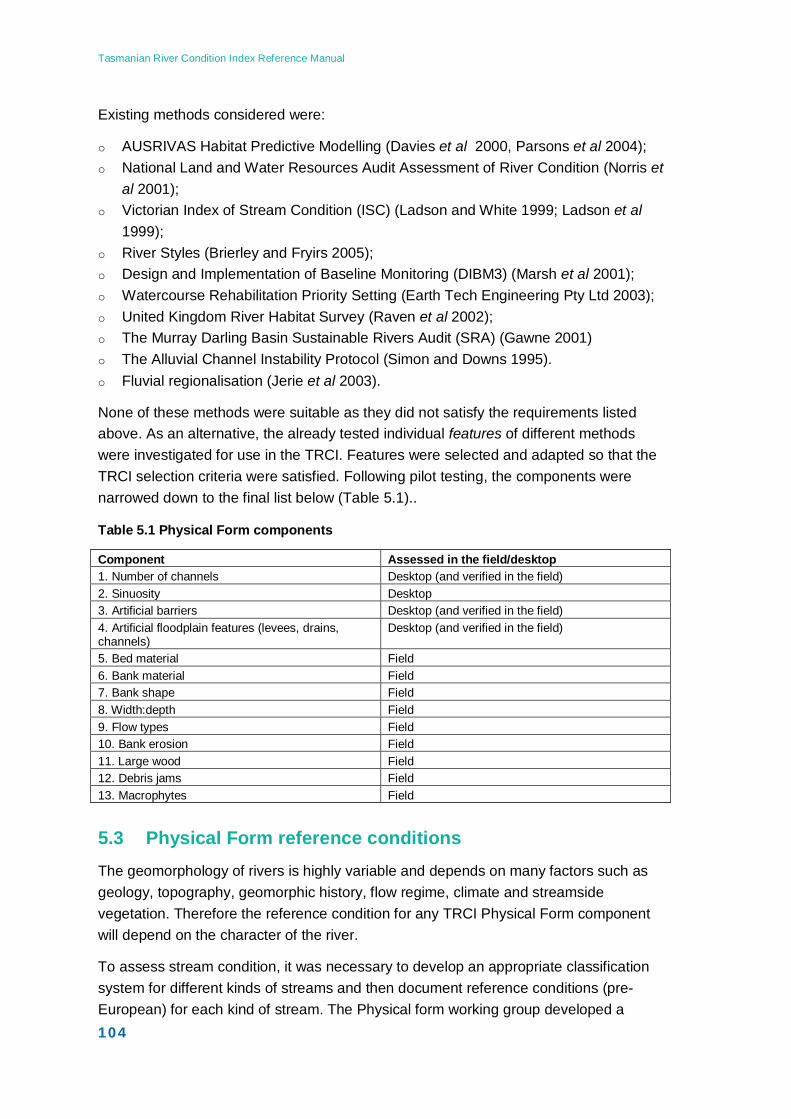
Tasmanian River Condition Index Reference Manual
104
Existing methods considered were:
o AUSRIVAS Habitat Predictive Modelling (Davies et al 2000, Parsons et al 2004); o National Land and Water Resources Audit Assessment of River Condition (Norris et
al 2001); o Victorian Index of Stream Condition (ISC) (Ladson and White 1999; Ladson et al
1999); o River Styles (Brierley and Fryirs 2005); o Design and Implementation of Baseline Monitoring (DIBM3) (Marsh et al 2001); o Watercourse Rehabilitation Priority Setting (Earth Tech Engineering Pty Ltd 2003); o United Kingdom River Habitat Survey (Raven et al 2002); o The Murray Darling Basin Sustainable Rivers Audit (SRA) (Gawne 2001) o The Alluvial Channel Instability Protocol (Simon and Downs 1995). o Fluvial regionalisation (Jerie et al 2003).
None of these methods were suitable as they did not satisfy the requirements listed above. As an alternative, the already tested individual features of different methods were investigated for use in the TRCI. Features were selected and adapted so that the TRCI selection criteria were satisfied. Following pilot testing, the components were narrowed down to the final list below (Table 5.1)..
Table 5.1 Physical Form components
Component Assessed in the field/desktop 1. Number of channels Desktop (and verified in the field) 2. Sinuosity Desktop 3. Artificial barriers Desktop (and verified in the field) 4. Artificial floodplain features (levees, drains, channels)
Desktop (and verified in the field)
5. Bed material Field 6. Bank material Field 7. Bank shape Field 8. Width:depth Field 9. Flow types Field 10. Bank erosion Field 11. Large wood Field 12. Debris jams Field 13. Macrophytes Field
5.3 Physical Form reference conditions The geomorphology of rivers is highly variable and depends on many factors such as geology, topography, geomorphic history, flow regime, climate and streamside vegetation. Therefore the reference condition for any TRCI Physical Form component will depend on the character of the river.
To assess stream condition, it was necessary to develop an appropriate classification system for different kinds of streams and then document reference conditions (pre-European) for each kind of stream. The Physical form working group developed a
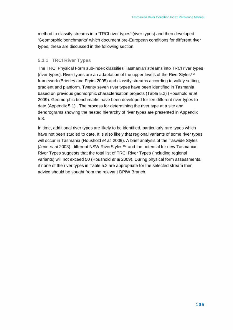
Tasmanian River Condition Index Reference Manual
105
method to classify streams into ‘TRCI river types’ (river types) and then developed ‘Geomorphic benchmarks’ which document pre-European conditions for different river types, these are discussed in the following section.
5.3.1 TRCI River Types The TRCI Physical Form sub-index classifies Tasmanian streams into TRCI river types (river types). River types are an adaptation of the upper levels of the RiverStyles™ framework (Brierley and Fryirs 2005) and classify streams according to valley setting, gradient and planform. Twenty seven river types have been identified in Tasmania based on previous geomorphic characterisation projects (Table 5.2) (Houshold et al 2009). Geomorphic benchmarks have been developed for ten different river types to date (Appendix 5.1) . The process for determining the river type at a site and dendrograms showing the nested hierarchy of river types are presented in Appendix 5.3.
In time, additional river types are likely to be identified, particularly rare types which have not been studied to date. It is also likely that regional variants of some river types will occur in Tasmania (Houshold et al. 2009). A brief analysis of the Taswide Styles (Jerie et al 2003), different NSW RiverStyles™ and the potential for new Tasmanian River Types suggests that the total list of TRCI River Types (including regional variants) will not exceed 50 (Houshold et al 2009). During physical form assessments, if none of the river types in Table 5.2 are appropriate for the selected stream then advice should be sought from the relevant DPIW Branch.
Tasmanian River Condition Index Reference Manual
106
Table 5.2 TRCI River Types
Valley setting TRCI River Types Benchmark developed Confined Confined steep Yes Confined low gradient Yes Steep gorge Yes Low gradient gorge Confined steep with occasional floodplain pockets Yes
Confined low gradient with occasional floodplain pockets
Yes
Moraine confined steep Moraine confined low gradient Talus confined steep Talus confined low gradient
Partly-confined Partly-confined beach ridge controlled discontinuous floodplain
Partly-confined bedrock controlled discontinuous floodplain
Yes
Partly-confined terrace controlled discontinuous floodplain
Partly-confined broadwater pool Partly-confined wandering planform controlled Partly-confined meandering planform controlled Yes Partly-confined planform controlled fan Yes Partly-confined low sinuosity planform controlled Yes Laterally-unconfined Laterally-unconfined intact valley fill
Laterally-unconfined discontinuous swamp belt Laterally-unconfined low sinuosity swamp channel Laterally-unconfined low sinuosity Yes Laterally-unconfined meandering Laterally-unconfined meandering swamp channel Laterally-unconfined bank confined Laterally-unconfined wandering Laterally-unconfined fan
5.3.2 TRCI Geomorphic Benchmarks Pre-European geomorphological conditions for different kinds of streams were not well documented and available for use in the TRCI. As a result, ‘Geomorphic benchmarks’ (benchmarks) have been developed for different river types. Benchmarks describe stream character, pre European conditions and likely degradation processes for each type. They also provide examples of moderate or poor condition in that particular river type to enable sites to be scored.
Only the most relevant components for a river type are scored (e.g. sinuosity is highly relevant as an indicator of degradation in laterally-unconfined settings, but not in confined river types).
During the development of benchmarks, pre-European conditions were defined conceptually using expert opinion, literature and data where available. Geomorphic benchmarks and a description of their development is presented in Appendix 5.1.
Tasmanian River Condition Index Reference Manual
107
5.3.3 River type change In the majority of cases it is expected that the current day river type is equivalent to the pre-European type. However, this cannot be assumed as local disturbance or activities in the catchment may have altered the geomorphology so much that a stream changes type (i.e. from a partly confined meandering stream to a partly confined low sinuosity stream). Data from the Conservation of Freshwater Ecosystem Values (CFEV) database is used to indicate catchment disturbance and hence the potential for river type change (from pre-European to the current day river type) at a particular site. A GIS shapefile has been developed which incorporates CFEV data including historic mining sedimentation, urbanisation next to the stream, unsealed road crossings, catchment disturbance and hydrological disturbance (Appendix 5.5). This tool gives a yes/no answer for each site as to potential for river type change. Type change is then identified, or verified using aerial photography, maps and historical data (Sections 5.6 and 5.7).
Sites are generally scored out of 100%. However, if river type change has occurred, the benchmark for the pre-European river type is used to score the site. The site is scored out of a maximum of 60%. If a particular stream is altered to the extent that a pre-European river type cannot be determined, the site is labelled as ‘heavily modified’ and a generic scoring system for these streams is used (Sections 5.6 and 5.7).
5.4 A Physical Form Assessment Site A Physical Form assessment site (site) generally starts at a riffle (or other stable control) and extends upstream. A riffle is a relatively stable feature within the channel, characterised by a rippled water surface under low flow conditions (Section 5.5.2.5). It is often located between two bends in a meandering river system.
The total length of a site is 15 x the bankfull width (measured at the start riffle). The site is comprised of 15 equally spaced transects across the stream. The first transect is located at the start riffle. The distance between transects is equal to the bankfull width measured at the start of the site.
The layout of a site is illustrated in Figure 5.1.
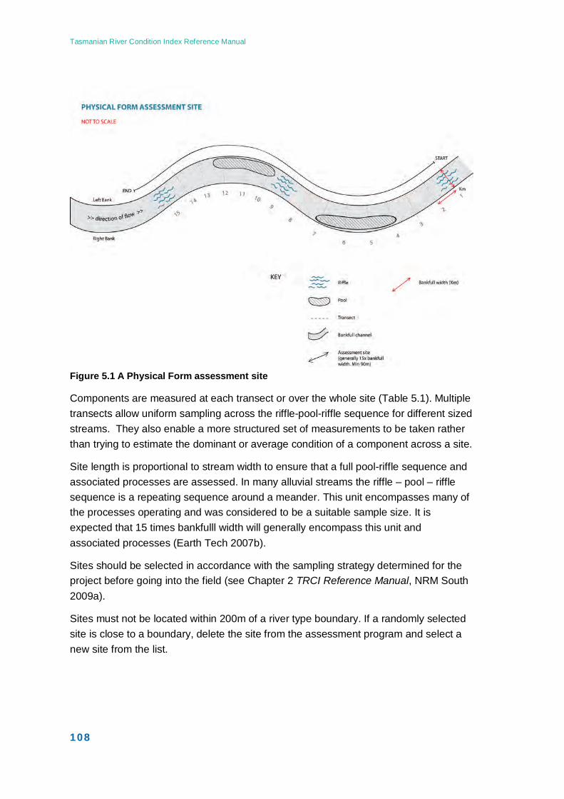
Tasmanian River Condition Index Reference Manual
108
Figure 5.1 A Physical Form assessment site
Components are measured at each transect or over the whole site (Table 5.1). Multiple transects allow uniform sampling across the riffle-pool-riffle sequence for different sized streams. They also enable a more structured set of measurements to be taken rather than trying to estimate the dominant or average condition of a component across a site.
Site length is proportional to stream width to ensure that a full pool-riffle sequence and associated processes are assessed. In many alluvial streams the riffle – pool – riffle sequence is a repeating sequence around a meander. This unit encompasses many of the processes operating and was considered to be a suitable sample size. It is expected that 15 times bankfulll width will generally encompass this unit and associated processes (Earth Tech 2007b).
Sites should be selected in accordance with the sampling strategy determined for the project before going into the field (see Chapter 2 TRCI Reference Manual, NRM South 2009a).
Sites must not be located within 200m of a river type boundary. If a randomly selected site is close to a boundary, delete the site from the assessment program and select a new site from the list.
Tasmanian River Condition Index Reference Manual
109
5.5 Description of components The components of the Physical Form sub-index are listed in Table 5.3 and described in the following section. The field assessment method is detailed in the Tasmanian River Condition Index Physical Form Field Manual (NRM South 2009c). Desktop methods are presented in Appendix 5.
Table 5.3 Physical Form components assessed in the field or at the desktop
Component Assessed in the field/desktop 1. Number of channels Desktop (and verified in the field) 2. Sinuosity Desktop 3. Artificial barriers Desktop (and verified in the field) 4. Artificial floodplain features (levees, drains, channels) Desktop (and verified in the field) 5. Bed material Field 6. Bank material Field 7. Bank shape Field 8. Width:depth Field 9. Flow types Field 10. Bank erosion Field 11. Large wood Field 12. Debris jams Field 13. Macrophytes Field
5.5.1 Desktop components The desktop components are assessed using maps, aerial photography and any historic survey plans that may be available for the area. The way in which they are measured is presented in Section 5.6. Desktop components, except sinuosity, may be verified in the field.
5.5.1.1 Number of channels
Streams in Tasmania are not all single channels, and vary from straight to anabranching (anastomosed) and/or braided channels. (Figure 5.2).
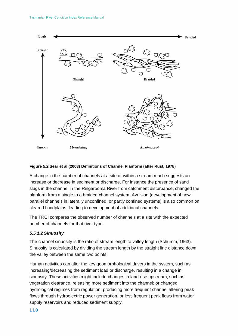
Tasmanian River Condition Index Reference Manual
110
Figure 5.2 Sear et al (2003) Definitions of Channel Planform (after Rust, 1978)
A change in the number of channels at a site or within a stream reach suggests an increase or decrease in sediment or discharge. For instance the presence of sand slugs in the channel in the Ringarooma River from catchment disturbance, changed the planform from a single to a braided channel system. Avulsion (development of new, parallel channels in laterally unconfined, or partly confined systems) is also common on cleared floodplains, leading to development of additional channels.
The TRCI compares the observed number of channels at a site with the expected number of channels for that river type.
5.5.1.2 Sinuosity
The channel sinuosity is the ratio of stream length to valley length (Schumm, 1963). Sinuosity is calculated by dividing the stream length by the straight line distance down the valley between the same two points.
Human activities can alter the key geomorphological drivers in the system, such as increasing/decreasing the sediment load or discharge, resulting in a change in sinuosity. These activities might include changes in land-use upstream, such as vegetation clearance, releasing more sediment into the channel; or changed hydrological regimes from regulation, producing more frequent channel altering peak flows through hydroelectric power generation, or less frequent peak flows from water supply reservoirs and reduced sediment supply.
Tasmanian River Condition Index Reference Manual
111
Stream channels may have also been altered to provide ‘better’ drainage or a more rapid escape for stormwater and associated pollutants. These channels have often been artificially channelized and straightened from their natural, more sinuous, state.
Sinuosity may naturally change in alluvial unconfined meandering streams with erodible bank material, as meander cutoffs isolate tight meanders from the active channel. However, this phenomenon would be accounted for in TRCI benchmarks.
In the TRCI, sinuosity is calculated by dividing the stream length (defined as the curvilinear distance measurement along the centre of the channel between two points) by the straight line distance down the valley between the same two points. The two points are defined as the upstream and downstream extent of the particular river type in which the site is located. Sinuosity measurements are made at the desktop using current 1:25,000 mapping or GIS information, such as the stream layers provided by CFEV, or aerial photography.
Sinuosity is only calculated for laterally unconfined river types. If multiple channels are present, sinuosity is not assessed as reference conditions are not currently available.
5.5.1.3 Artificial barriers
Artificial barriers include weirs, dams and road culverts that act as an element of ‘roughness’ in the stream, altering the flow of water within the channel. Barriers such as online farm dams can influence the boundary roughness by acting as artificial channel bed controls, potentially causing scour downstream and aggradation upstream.
In the TRCI, the presence of artificial barriers (none; partial (> 50%); or total blockage) in the bankfull stream cross-sectional area is recorded at each site.
5.5.1.4 Artificial floodplain features (levees, drains and channels)
Artificial floodplain features are constructed levees, drains and channels on the floodplain. These features change the geomorphology of both the channel and the floodplain. In the case of artificial levee development the floodplain will be disconnected from the channel. This means that high flows will no longer have their energy dissipated on the floodplain and the likelihood of in-channel erosion increases.
Drains reduce the storage time of water on the floodplain, the decreased lag time may result in a higher flood peak within the channel and a potentially increased sediment supply.
In the TRCI, artificial floodplain features are recorded along the length of the river type in which the site is located. While this component is assessed at every site, it is only likely to be relevant and hence scored, in laterally unconfined or partly confined river types.
Tasmanian River Condition Index Reference Manual
112
5.5.2 Field components assessed at transects 5.5.2.1 Bed material
Bed material is assessed by recording the different sediment size classes present in the stream at a site and comparing them with the expected sediment size classes. Assessing the bed material provides information about changes in roughness, bed diversity and habitat.
Bed material change may occur when the natural bed sediment supply is disrupted, such as downstream of a reservoir or where the bed is homogenised by a sand slug.
On site, the dominant, sub dominant and present bed material is recorded at each transect. This is then tallied to give the average dominant, sub-dominant and other sediment size classes present at a site. The sediment size classes and definitions are:
o Bedrocko
is generally a consistent layer of rock, rather than separate particles; Boulders
o
are generally larger than the size of your head (>256 mm); Cobbles
o
range from approximately tennis ball size up to volley ball size (64-256 mm); Pebbles
o
range from approximately pea to tennis ball size (16 – 64 mm); Gravel
o
ranges from approximately pin heads to pea size (2-16 mm); Sands
o
are approximately pin-head size (0.06-2 mm); Fines
o
consists of silts, clays, muds (<0.06 mm); Artificial
5.5.2.2 Bank material
is any material anthropogenically placed or growing in the channel i.e. concrete, brick, willow roots.
This information aids in confirming the TRCI River Type at a site. For instance, bedrock and boulder would be expected in a confined valley setting. However, the widespread presence of such material within laterally-unconfined valley settings would highlight the need for further investigation. Secondly, comparison of bank material with other field components such as bed material and bank erosion can provide insight into any degradation processes occurring, such as the presence of a sand slug (bed material) within a channel consisting of bedrock/boulder banks.
Bank material information also assists in the interpretation of the bank shape component. Steep and vertical banks consisting of earth or clay indicate very different conditions to steep and vertical banks comprised of large boulders.
The bank material is recorded (left and right bank) at each transect. Using this information, the dominant bank material for each site is determined.
Tasmanian River Condition Index Reference Manual
113
Bank materials and definitions are listed below:
o NV = not visible o BE = bedrock o BO = boulder (>256 mm) o CO = cobble (64-256mm) o PE = pebble (16mm-64mm) o GS = gravel/sand (0.06-16mm) o EA = earth o CL = sticky clay o AR = artificial (concrete, iron, gabion, brick, rip rap, urban rubble)
Whilst not wishing to deter field operators from a full investigation of the site, the NV category is available so that operators do not feel the need to ‘invent’ data.
5.5.2.3 Bank shape
The shape, or cross-sectional profile, of the bank gives an indication of the flux of sediment in and out of the channel as well as bank and riparian vegetation interactions with flow and channel sediment.
When the supply of sediment from upstream is greater than the erosion (input > output) then aggradation may occur at the bank toe and the bank profile may become stepped (C), gentle (G) or benches and bars may form (B) (refer descriptions and codes below). If the quantity of sediment coming in is similar to that being eroded (input = output), then the banks tend to remain static and have little in the way of undercuts (V). When bank failure occurs, locally derived material accumulates at the bank toe (VT). When erosion dominates over the incoming sediment (inputs<outputs) then the banks tend to become vertical or undercut (VU). This is termed basal endpoint control (Thorne, 1982) as it is assumed that the controlling area for the bank is at the base, or contact between the bed and banks. What happens in this region will influence the overlying bank material.
In the TRCI, the dominant shape of the left and the right bank is recorded along each site. If it is difficult to determine the extent of the bank then the basal area of the bank is the subject of the assessment.
Tasmanian River Condition Index Reference Manual
114
Bank shapes and definitions are listed below:
o V = Vertical (with no undercut or slumped toe material) o U = undercut (predominantly vertical bank) o VT = Vertical (vertical bank with slumped material at toe) o S = Steep (steep bank >45 degrees, but not vertical) o G = Gentle (gentle <45 degrees) o C = Composite (composite, complex profile) o B = Berm (natural berm, transitional feature) o RS = Resectioned (bank profile modified, resectioned, reprofiled) o AR = Artificial (bank artificially strengthened for bank protection purposes i.e.
concrete, rip rap, urban rubble)
5.5.2.4 Bankfull width:depth ratio
Bankfull is defined as the lowest point at which the channel breaks out on to the floodplain, or floodplain pockets. Other clues that may indicate the channel maintenance flow level include a break in slope, flood trashlines, sediment lines on bridges, vegetation limits or lichen lines on boulders and bedrock outcrops. These may be particularly useful in confined stream settings.
Bankfull width is the width of the channel at bankfull discharge. This represents a standard measure of channel dimension, rather than using the width of the water at the cross-section at the time of measurement, which may vary with different stage heights. Channel erosion can increase the width of the stream, especially those that have a very shallow depth to bedrock. Channels may become narrower as a result of willow encroachment encouraging channel deposition and accretion of benches and lateral bars.
Bankfull depth is defined as the distance between the top of the riffle crest (the shallowest part of the riffle or control point in the channel) and the height of the bankfull width measurement. This represents a standard measure of channel dimension, rather than the stage dependent measure of wetted depth. Bed incision can increase the depth of the stream, especially in laterally-unconfined valleys where the streams come into contact with material with low shear strength. Building artificial levees can also cause the channel to be constrained and incised. Deposition of sediment within the channel because of increased bed loads (for example sand slugs) will cause the depth of the stream to decrease. This is likely to be accompanied by a corresponding widening of the channel in order to transport the same flows.
Bankfull width and bankfull depth are important condition measures but they can be strongly influenced by catchment area, so the TRCI uses the width:depth ratio in scoring.
The bankfull width is measured using a range finder or tape measure and recorded on the data sheet at every transect. Depth should be measured at riffles, or shallow points
Tasmanian River Condition Index Reference Manual
115
of the channel for practical and safety reasons, and recorded on the data sheet. The average bankfull width:depth ratio at the site is then calculated and recorded on the data sheet.
5.5.2.5 Flow types
Flow types are distinct patches in the surface flow character of the stream that are caused by differences in hydraulic character (Newson & Newson, 2000). Examples of flow types are rippled flow or unbroken standing waves. These simply measured hydraulic characteristics are used as surrogates for more extensive measures of roughness such as riffles, pools or cascades. The abundance or diversity of flow types present at the assessment site is to be compared with the expected abundance or diversity of flow types for that River Type.
A departure from the expected abundance or diversity of flow types may indicate a change in the amount of sediment entering or leaving the system due to a change in the system drivers and hence bedforms. For example a sand slug may drown out all the pools and riffles leaving a single flow type throughout the site. There is also the ability for the site to have a higher input of the expected sediment by anthropogenic activity upstream, construction of bridges or drainage channels, releasing a higher volume of the existing (expected) bed sediment into the channel. In these cases whilst the hydrology and bed material may stay the same and the channel dimensions may not change appreciably, the bedforms may change. This would be indicated by the flow types observed.
Flow types and examples of how they are expressed as river features are listed below.
o FF = Free fall (waterfall) o CH = Chute (cascade, step) o BW = Broken standing waves (rapid, cascade) o UW = Unbroken standing waves (riffle) o CF = Chaotic flow (a combination of any of the flow types) o RP = Rippled (run) o UP = Upwelling (boil) o SM = Smooth (smooth boundary, glide) o NP = No perceptible flow (pool, deadwater on margins, bends, downstream of point
bars and other obstructions) o NO = no flow
In the TRCI, the presence of different surface flow types is recorded at each transect (flow types must intersect the transect line, so it is as if you have a piece of string stretched across the river and you count each flow type that is crossed by the line).To ensure accurate comparisons over time it is important to record the ‘water level at the time of sampling’ on the physical form data sheet to assist as flow types will vary depending on the depth of the flow in the channel.
Tasmanian River Condition Index Reference Manual
116
5.5.3 Field components assessed over whole site 5.5.3.1 Bank erosion
Increased or decreased bank erosion may indicate a change in sediment loads, flows or bank stability. This component records the area of active and recently eroding surfaces on the banks of the whole site. It is restricted to larger scale erosion scars and mass failures as these features are easier to identify consistently between observers. The proportion of eroded bank at a site is compared to the expected proportion for the particular river type, as erosion is expected in some river types.
Bank erosion is recorded after the transect-based assessments. As assessors walk back through the site, the length and height of active, recent erosion scars are recorded along each bank (with the exception of discontinuous occurrences <0.5m2 ).
5.5.3.2 Large wood
Large wood is defined as dead trees or branches in the stream channel that are greater than 0.1m in diameter and greater than 1m long. Large wood in a stream can influence stream geomorphology because it is a resistance or ‘roughness’ element that can add friction to the flow, influencing flow velocities. The presence of large wood in a stream changes the hydraulic environment that surrounds it, resulting in scour, and/or aggradation.
In the TRCI, the number of pieces of large wood are recorded, along the length of the assessment site. The large wood score is obtained by comparing the ‘observed’ quantity of large wood in a stream with the ‘expected’ amount of large wood in the particular river type.
5.5.3.3 Debris jams
Debris jams are accumulations of two or more pieces of large wood within the channel. They influence stream geomorphology through changing flow velocities, scour and/or aggradation. In the TRCI, the number of debris jams along the site are recorded. These are categorised as filling less than 50% or greater than 50% void space in a bankfull channel cross-section.
5.5.3.4 Emergent macrophytes
Emergent macrophytes are aquatic plant species (such as Cumbungi Typha spp., Reeds Phragmites australis, and Rushes Juncus spp.) which grow in the stream bed and have leaves emerging above the water surface. They provide an element of ‘roughness’ in the stream. This indicator is independent of whether the macrophyte is exotic or native as we are only considering the geomorphic effects of added or lost roughness not the invasion of alien species for ecological purposes.
The proportion of the low flow channel bed within the whole site, that supports macrophyte coverage is visually estimated and recorded on the data sheet.

Tasmanian River Condition Index Reference Manual
117
5.6 Summary of Assessment Procedure The assessment procedure is summarised below:
1. Design assessment program: planning, training, assessment preparation;
2. Select sites;
3. Collect desktop information for each site, including CFEV information;
4. Determine pre-European river type;
5. Conduct site assessments;
6. Complete data entry, assessment of desktop components, analysis and scoring for each component;
7. Calculate Physical Form score for site;
8. Calculate Physical Form score for reporting unit.
The design of a TRCI assessment program, sampling strategy and site selection are detailed in Chapter 2 of this document.
Sampling timing, training and resources required are discussed below. This is followed by the desktop and field assessment methods and data entry. Finally the scoring for each component, integrating these to a Physical Form score for a site and the method for calculating the Physical Form score for the reporting unit (i.e. sub-catchment) are described.
5.6.1 Sampling timing It is recommended that Physical Form assessments are completed in Summer or Autumn or when flows are low, to ensure maximum visibility of bed and bank features.
It is also suggested that Physical Form assessments be completed in conjunction with Streamside Zone assessments, by the same team of two people, to reduce field assessment costs and increase efficiency.
5.6.2 Training Determination of river type and type change must be completed by a trained geomorphologist, in consultation with DPIW geomorphologists.
The completion of desktop components and field assessment should be conducted by personnel who have been trained by a geomorphologist.
Contact NRM South to find trained personnel or enquire about training opportunities.
Tasmanian River Condition Index Reference Manual
118
5.6.3 Resources required 5.6.3.1 Desktop assessment
The following maps and data are required to determine river type and to complete the desktop components (Number of channels, Sinuosity, Artificial barriers and Artificial floodplain features) of the method.
o TRCI River Typing method, River Type list and dendrograms (Appendix 5.3) o Existing TasWide Styles/ RiverStyles™ mapping and DPIW Rivercare Plans if
available o Fluvial Landscape Mosaic (FLM) mapping (Jerie et al 2003) o 1:25,000 topographic maps o Colour 1:25 000 aerial imagery of the assessment area (1:42 000 if finer resolution
is unavailable) and a stereoscope o TRCI CFEV shapefile to indicate potential for type change (available from NRM
South) o CFEV database to determine slope for confined river types o A DEM where possible o Historical data, early aerial photos, survey plans and maps if available from
DPIW/LIST to identify planform changes over time (if river type change is suspected)
5.6.3.2 Field assessment
Equipment required for TRCI Physical Form and Streamside Zone field assessments is listed below:
o Camera o GPS o Range finder o Clinometer o Depth staff o 30 m tape measure o Data sheets (including some on waterproof paper) and clipboard o Assessment program information letters for landholders o 1:25,000 TasMaps o Site location maps
5.6.3.3 Data Analysis
The data collected at each site is entered into the TRCI Database.
Sites are scored using the appropriate scoring table for the river type in which the site is located. Scoring tables are included in the geomorphic benchmarks and in Excel spreadsheet form. Geomorphic benchmarks and scoring tables are presented in Appendix 5.2. Excel workbooks are available from NRM South.
Tasmanian River Condition Index Reference Manual
119
5.7 Methods Sites should be selected using one of the options outlined in Chapter 2. The pre-European river type for each site is then determined (Appendix 5 and summarised below), followed by field and desktop assessments. Detailed methods are presented in NRM South (2009c) and Appendix 5.
5.7.1.1 Determining pre- European TRCI River Type
The procedure for determining river type is summarised below (Appendix 5.3). The determination of river type should only ever be completed by a trained geomorphologist. Fluvial geomorphologists at DPIW will be able to provide advice on determining river types. This will ensure a uniform approach to river typing, enable the list of river types to be maintained by DPIW and new benchmarks developed and disseminated as required.
The river typing procedure systematically identifies river types according to a hierarchy of controls based on valley confinement, gradient and planform (aided in some cases by instream geomorphic units). Bed and bank materials are not used, as they cannot be remotely assessed at the desktop. The steps to determine a river type are:
1. Collect resources (maps, aerial photography, refer Section 5.6.2);
2. Collect data for the site:
a. ‘potential for river type change’ (yes/no) from TRCI Arc GIS shapefile;
b. slope (where steep is > 0.1 m m-1, and moderate-low is < 0.1 m m-1) ;
c. CFEV stream order for each site;
3. Identify floodplain planform distribution;
4. Identify valley setting (confined/partly confined/laterally unconfined and percentage of channel length in contact with valley margin);
5. Confirm river gradient (steep or moderate-low);
6. Identify channel planform (number of channels and sinuosity);
7. Assign a pre-European river type to the site, or contact DPIW if a new type is suspected. Map the full extent of the type immediately surrounding the site. If the TRCI GIS shapefile suggests that there is potential for river type change at a site, verify using aerial photography, historical maps and data. Sites are generally scored out of 100%. However, if river type change has occurred, the benchmark for the pre-European river type is used to score the site. The site is scored out of a maximum of 60%. If a particular stream is altered to the extent that a pre-European river type cannot be determined, the site is labelled as
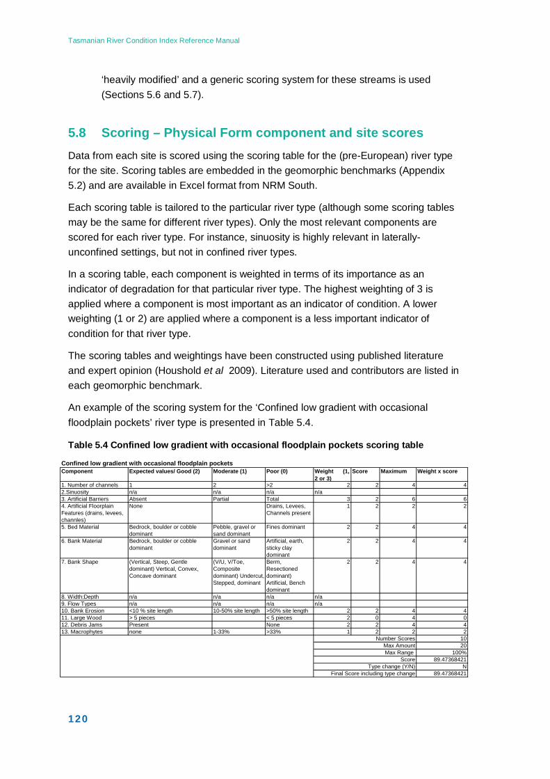
Tasmanian River Condition Index Reference Manual
120
‘heavily modified’ and a generic scoring system for these streams is used (Sections 5.6 and 5.7).
5.8 Scoring – Physical Form component and site scores Data from each site is scored using the scoring table for the (pre-European) river type for the site. Scoring tables are embedded in the geomorphic benchmarks (Appendix 5.2) and are available in Excel format from NRM South.
Each scoring table is tailored to the particular river type (although some scoring tables may be the same for different river types). Only the most relevant components are scored for each river type. For instance, sinuosity is highly relevant in laterally-unconfined settings, but not in confined river types.
In a scoring table, each component is weighted in terms of its importance as an indicator of degradation for that particular river type. The highest weighting of 3 is applied where a component is most important as an indicator of condition. A lower weighting (1 or 2) are applied where a component is a less important indicator of condition for that river type.
The scoring tables and weightings have been constructed using published literature and expert opinion (Houshold et al 2009). Literature used and contributors are listed in each geomorphic benchmark.
An example of the scoring system for the ‘Confined low gradient with occasional floodplain pockets’ river type is presented in Table 5.4.
Table 5.4 Confined low gradient with occasional floodplain pockets scoring table
Confined low gradient with occasional floodplain pockets Component Expected values/ Good (2) Moderate (1) Poor (0) Weight (1,
2 or 3)Score Maximum Weight x score
1. Number of channels 1 2 >2 2 2 4 42.Sinuosity n/a n/a n/a n/a3. Artificial Barriers Absent Partial Total 3 2 6 64. Artificial Floorplain Features (drains, levees, channles)
None Drains, Levees, Channels present
1 2 2 2
5. Bed Material Bedrock, boulder or cobble dominant
Pebble, gravel or sand dominant
Fines dominant 2 2 4 4
6. Bank Material Bedrock, boulder or cobble dominant
Gravel or sand dominant
Artificial, earth, sticky clay dominant
2 2 4 4
7. Bank Shape (Vertical, Steep, Gentle dominant) Vertical, Convex, Concave dominant
(V/U, V/Toe, Composite dominant) Undercut, Stepped, dominant
Berm, Resectioned dominant) Artificial, Bench dominant
2 2 4 4
8. Width:Depth n/a n/a n/a n/a9. Flow Types n/a n/a n/a n/a10. Bank Erosion <10 % site length 10-50% site length >50% site length 2 2 4 411. Large Wood > 5 pieces < 5 pieces 2 0 4 012. Debris Jams Present None 2 2 4 413. Macrophytes none 1-33% >33% 1 2 2 2
1020
100%89.47368421
N89.47368421
Number ScoresMax AmountMax Range
ScoreType change (Y/N)
Final Score including type change
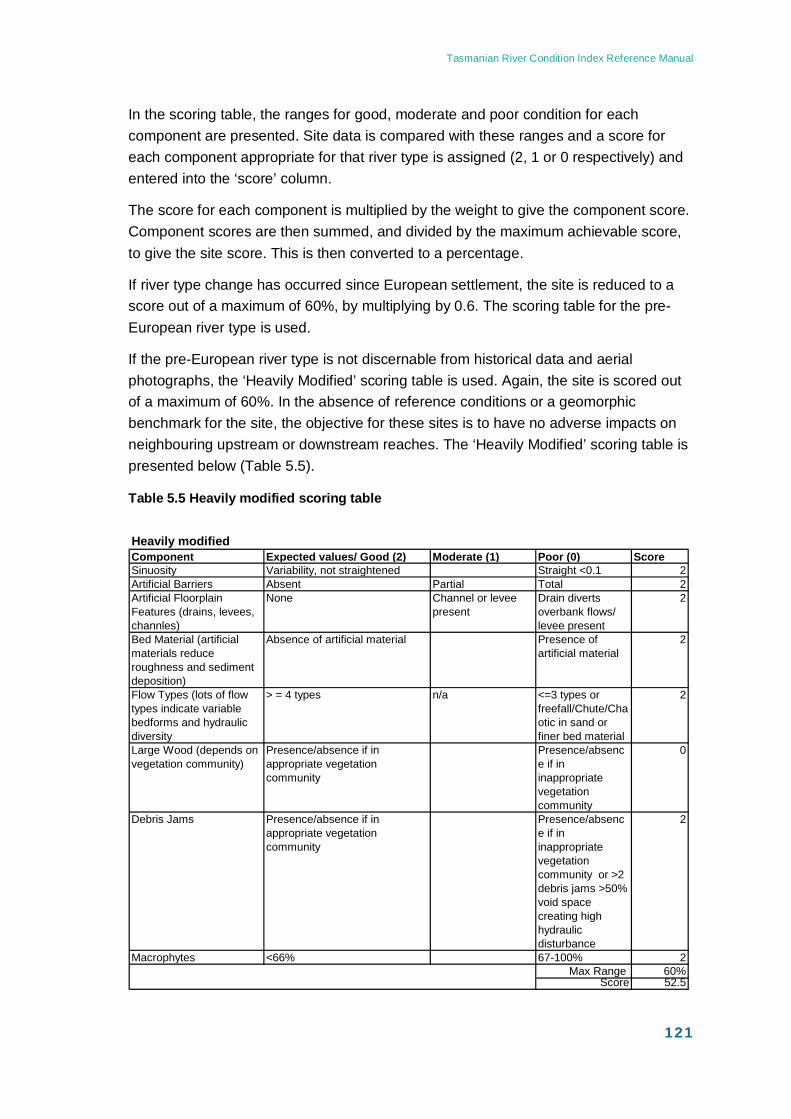
Tasmanian River Condition Index Reference Manual
121
In the scoring table, the ranges for good, moderate and poor condition for each component are presented. Site data is compared with these ranges and a score for each component appropriate for that river type is assigned (2, 1 or 0 respectively) and entered into the ‘score’ column.
The score for each component is multiplied by the weight to give the component score. Component scores are then summed, and divided by the maximum achievable score, to give the site score. This is then converted to a percentage.
If river type change has occurred since European settlement, the site is reduced to a score out of a maximum of 60%, by multiplying by 0.6. The scoring table for the pre-European river type is used.
If the pre-European river type is not discernable from historical data and aerial photographs, the ‘Heavily Modified’ scoring table is used. Again, the site is scored out of a maximum of 60%. In the absence of reference conditions or a geomorphic benchmark for the site, the objective for these sites is to have no adverse impacts on neighbouring upstream or downstream reaches. The ‘Heavily Modified’ scoring table is presented below (Table 5.5).
Table 5.5 Heavily modified scoring table
Heavily modifiedComponent Expected values/ Good (2) Moderate (1) Poor (0) ScoreSinuosity Variability, not straightened Straight <0.1 2Artificial Barriers Absent Partial Total 2Artificial Floorplain Features (drains, levees, channles)
None Channel or levee present
Drain diverts overbank flows/ levee present
2
Bed Material (artificial materials reduce roughness and sediment deposition)
Absence of artificial material Presence of artificial material
2
Flow Types (lots of flow types indicate variable bedforms and hydraulic diversity
> = 4 types n/a <=3 types or freefall/Chute/Chaotic in sand or finer bed material
2
Large Wood (depends on vegetation community)
Presence/absence if in appropriate vegetation community
Presence/absence if in inappropriate vegetation community
0
Debris Jams Presence/absence if in appropriate vegetation community
Presence/absence if in inappropriate vegetation community or >2 debris jams >50% void space creating high hydraulic disturbance
2
Macrophytes <66% 67-100% 2Max Range 60%
Score 52.5
Tasmanian River Condition Index Reference Manual
122
It is the aim of the TRCI that site and reporting unit scores correspond with the FARWH bands and ratings to enable reporting on condition at the National level. However this has not been fully tested in the Physical Form sub-index due to the limited availability of geomorphic benchmarks and scores for sites. Further testing and refinement of benchmarks and the method should aim to ensure compatibility with the FARWH bands and ratings presented below (Table 5.6).
Table 5.6 FARWH Bands and Ratings
Score Rating 0-0.2 Severely modified condition 0.2-0.4 Substantially modified condition 0.4-0.6 Moderately modified condition 0.6-0.8 Slightly modified condition 0.8-1 Largely unmodified condition
5.8.1 Physical Form score for a reporting unit The Physical Form sub-index score for the reporting unit (i.e. sub-catchment) is obtained by taking the median of all site scores in the sub-catchment. A minimum number of sites must be assessed before making this calculation. Refer Chapter 2.
5.9 Future assessments and the development of additional benchmarks Physical Form is a key aspect of river condition and the TRCI. Given the current status of the Physical Form method and the limited number of geomorphic benchmarks, future assessments and testing of the physical form method should be completed in consultation with NRM South and in conjunction with DPIW. This will ensure a co-ordinated approach to data management, desktop river typing, the development of further geomorphic benchmarks and regional variants, the scoring of physical form data and the dissemination of data and information.
5.10 References - Physical Form Brierley, G.J. and Fryirs, K.A. (2005) Geomorphology and River Management: Applications of the RiverStyles™ Framework. Blackwell Science, Oxford, UK.
Davies, N.M., Norris, R.H. and Thoms, M.C. (2000) Prediction and assessment of local stream habitat features using large-scale catchment characteristics. Freshwater Biology, 45: 343-370.
Tasmanian River Condition Index Reference Manual
123
Earth Tech Engineering Pty Ltd, (2003) Watercourse rehabilitation Priority Setting Process. Report for Northern Adelaide and Barossa, Onkaparinga, Patawolonga and Torrens Catchment Water Management Boards.
Gawne, B. (2001) Review and development of physical habitat assessment protocols. In: Whittington et al. (eds) Development of a framework for the Sustainable Rivers Audit. Technical Report #8/2001. Cooperative Research Centre for Freshwater Ecology, Canberra.
Houshold, I., Grove, J., Spink, A. and Slijkerman, J. (2009) Tasmanian River Condition Index: Revised Physical Form Method and Application in the Leven catchment. A report to NRM South. DPIW. Hobart.
Jerie, K., Houshold, I., and Peters, D. (2003) Tasmania’s river geomorphology: stream character and regional analysis, Volume 1. Department of Primary Industries, Water and Environment.
Ladson, A.R., White, L.J., Doolan, J.A., Finlayson, B.L., Hart, B.T., Lake, P.S. and Tilleard, J.W. (1999) Development and testing of an Index of Stream Condition for waterway management in Australia. Freshwater Biology, 41: 453-468.
Ladson, A. R. and White, L. J. (1999) Index of stream condition: reference manual. Department of Natural Resources and Environment.
Marsh, N., Coysh, J, Smith, M., Davies, N., Norris, R., Clapcott, J. (2001) Assessment of Channel Morphology and Development of a Predictive Habitat Assessment Model. Design and Implementation of Baseline Monitoring (DIBM3) Final Report.
Newson MD, Newson CL. (2000) Geomorphology, ecology and river channel habitat: mesoscale approaches to basin scale challenges. Progress in Physical Geography 24: 195-217.
Norris, R. H., Young, B., Liston, P., Bauer, N., Davies, N., Dyer, F., Linke, S. and Thoms, M. (2001) The assessment of river condition: an audit of the ecological condition of Australian Rivers. National Land and Water Resources Audit.
Parsons, M., Thoms, M. C. and Norris, R. H. (2004) Development of a standardised approach to river habitat assessment in Australia. Environmental Monitoring and Assessment 98:109-130.
Raven, P. J., Holmes, N.T.H., Charrier, P., Dawson, F.H., Naura, M, and Boon, P.J. (2002) Towards a harmonized approach for hydromorphological assessment of rivers in Europe: a qualitative comparison of three survey methods. Aquatic Conservation-Marine and Freshwater Ecosystems, 12: 405-424.
Simon, A. and Downes, P.W. (1995) An interdisciplinary approach to evaluation of potential instability in alluvial channels. Geomorphology, 12: 215-232.

Tasmanian River Condition Index Reference Manual
124
Thorne, C.R. (1982) Processes and mechanisms of river bank erosion. In Hey, R.D., Bathurst, J.C. and Thorne, C.R. (Eds), Gravel Bed Rivers, Wiley, Chichester, 227-259.
Whittington, J., Coysh, J., Davies, P., Dyer, F., Gawne, B., Lawrence, I., Liston, P., Norris, R., Robinson, W. and Thoms, M. (2001) Development of a Framework for the Sustainable Rivers Audit. Technical Report no. 8/2001. Cooperative Research Centre for Freshwater Ecology, Canberra

Tasmanian River Condition Index Reference Manual
125

Tasmanian River Condition Index Reference Manual
126
Appendix to Chapter 5: Further detail on the Physical Form sub-index Appendix 5.1 Development of Geomorphic Benchmarks
Appendix 5.2 Geomorphic Benchmarks
Appendix 5.3 Method for Determining TRCI River Type
Appendix 5.4 River Type Dendrograms
Appendix 5.5 CFEV Information Used to Indicate the Potential for River Type Change
Appendix 5.6 Physical Form Desktop Component Assessment Methods
Appendix 5.7 Physical Form Datasheets
Tasmanian River Condition Index Reference Manual
127
Appendix 5.1 The Development of Geomorphic Benchmarks Geomorphic benchmarks describe the pre-European character of river types and ways in which local and catchment disturbance are likely to affect key components measured at test sites. Conceptual models of character and behaviour inform scoring tables developed for each type, allowing quantification of the departure of test sites from reference condition. Benchmarks developed to date are listed in Appendix 5.2.
Each benchmark is a simple document (approximately two pages) comprising two parts:
o Section 1 provides context through a description of geomorphic controls, physical attributes and hydro-geomorphology of each river type in pre-European condition. It also presents a conceptual model of processes leading to degradation, appropriate to that type. This provides a theoretical basis for a referential scoring system.
o Section 2 provides a scoring system for each river type. Score ranges for good (expected), moderately and badly degraded condition are provided for a suite of field components relevant to that type. The score for each component is then ranked according to its importance with respect to type, and confidence in the data.
Geomorphic benchmarks are developed using literature review, (eg Knighton 1998, Kondolf & Piegay 2003, Brierley & Fryirs 2005), Taswide Styles descriptions (Jerie et. al 2003), adaptation of NSW River Styles references (eg Outhet & Young 2006), expert opinion and field data collected from sites in ‘near natural’ condition, assessed during pilot testing. These sites were selected according to the following criteria:
o high CFEV naturalness scores; o correspondence with historical mapping and air photos (at the desktop level); o field indicators, including the age of streamside vegetation and expected levels of
bank erosion for each river type; and o presence/absence of key, expected geomorphic units for that type.
Score ranges reflecting specifically Tasmanian contexts are broadly guided by data collected during previous Tasmanian Rivercare programs (eg Lampert 2000), academic research (eg Stronach 2000) and associated classification projects (eg Jerie et. al 2003).
As with stream classification (see Appendix 5.3), key attributes of Fluvial Landscape Mosaics (Jerie et. al 2003) may be used to inform the development of benchmarks for important regional variants of river types. Where FLMs suggest that regional variation in bed and bank materials (or other field measures) is highly likely, such as in a river type found in both granite and dolerite catchments, or in karst or glaciated terrain, different score ranges will be required for each variant. FLM attributes may also be used to support development of benchmarks for bed and bank grainsize (due to lithological variation), presence of large wood (eg alpine vs forest context), flow types (eg karst streams), and width:depth ratios (eg peatland streams).
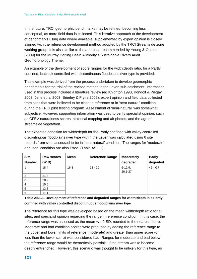
Tasmanian River Condition Index Reference Manual
128
In the future, TRCI geomorphic benchmarks may be refined, becoming less conceptual, as more field data is collected. This iterative approach to the development of benchmarks using data where available, supplemented by expert opinion is closely aligned with the reference development method adopted by the TRCI Streamside zone working group. It is also similar to the approach recommended by Young & Outhet (2009) for the Murray Darling Basin Authority’s Sustainable Rivers Audit Geomorphology Theme.
An example of the development of score ranges for the width:depth ratio, for a Partly confined, bedrock controlled with discontinuous floodplains river type is provided.
This example was derived from the process undertaken to develop geomorphic benchmarks for the trial of the revised method in the Leven sub-catchment. Information used in this process included a literature review (eg Knighton 1998, Kondolf & Piegay 2003, Jerie et. al 2003, Brierley & Fryirs 2005), expert opinion and field data collected from sites that were believed to be close to reference or in ‘near natural’ condition, during the TRCI pilot testing program. Assessment of ‘near-natural’ was somewhat subjective. However, supporting information was used to verify specialist opinion, such as CFEV naturalness scores, historical mapping and air photos, and the age of streamside vegetation.
The expected condition for width:depth for the Partly confined with valley controlled discontinuous floodplains river type within the Leven was calculated using 6 site records from sites assessed to be in ‘near natural’ condition. The ranges for ‘moderate’ and ‘bad’ condition are also listed. (Table A5.1.1).
Site Number
Raw scores (W:D)
Mean Reference Range Moderately degraded
Badly degraded
1 18.4
16.8 13 - 20 6-12.9; 20.1-27
<6: >27
2 21.8 3 20.2 4 15.5 5 13.3 6 11.1
Table A5.1.1. Development of reference and degraded ranges for width:depth in a Partly confined with valley controlled discontinuous floodplains river type
The reference for this type was developed based on the mean width:depth ratio for all sites, and specialist opinion regarding the range in reference condition. In this case, the reference range was assessed as the mean +/-- 2 SD, rounded to the nearest metre. Moderate and bad condition scores were produced by adding the reference range to the upper and lower limits of reference (moderate) and greater than upper score (or less than the lower score) was considered bad. Ranges for moderate and bad below the reference range would be theoretically possible, if the stream was to become deeply entrenched. However, this scenario was thought to be unlikely for this type, as
Tasmanian River Condition Index Reference Manual
129
its gradient is generally constrained by closely spaced bedrock bars, limiting the potential for bed incision. It is far more likely that this type would experience widening and even infilling as streamside vegetation is disturbed, and catchment erosion increased sediment supply. These data are supported by research in similar river types in comparable contexts (eg Brierley & Fryirs 2005).
This example illustrates the use of Section 1 of the geomorphic reference (the conceptual model) in providing contextual information for the expected width:depth ratio of this type, and its likely degradation trajectory. It uses field data, literature and interpretation of the conceptual model to estimate good (expected), moderate and badly degraded score ranges for the width:depth component of this type.
Other components of the scoring table have been developed in a similar way where field data was available, however in many cases greater reliance was put on published literature relating to each component, as use of local specialist knowledge to help ensure that this aligned with Tasmanian conditions. As the method is developed for other river types across a range of catchments catchments and contexts in future, more reliance on local field data will be possible.
References
Brierley, G.J. and Fryirs, K.A. (2005) Geomorphology and River Management: Applications of the RiverStyles Framework. Blackwell Science, Oxford, UK.
Jerie, K., Houshold, I., and Peters, D. (2003) Tasmania’s River Geomorphology: Stream Character and Regional Analysis, Volume 1. Department of Primary Industries, Water and Environment. Hobart.
Knighton, A.D. (1998) Fluvial Forms and Processes : A New Perspective.
Kondolf, G.M. and Piegay, H. (2003) Tools in fluvial geomorphology. Wiley, Chichester
Lampert, G. (2000) River Styles in the Mersey catchment, north west Tasmania. Macquarie Research Ltd.
Outhet, D. and Young, C. (2009) Sustainable Rivers Audit: Field Manual For Monitoring Stream Channel Geomorphic Condition. January 2009 Draft for Review
Rosgen, D.L. (1994) A classification of natural rivers. Catena 22(3): 169-199.

Tasmanian River Condition Index Reference Manual
130
Appendix 5.2 Geomorphic Benchmarks
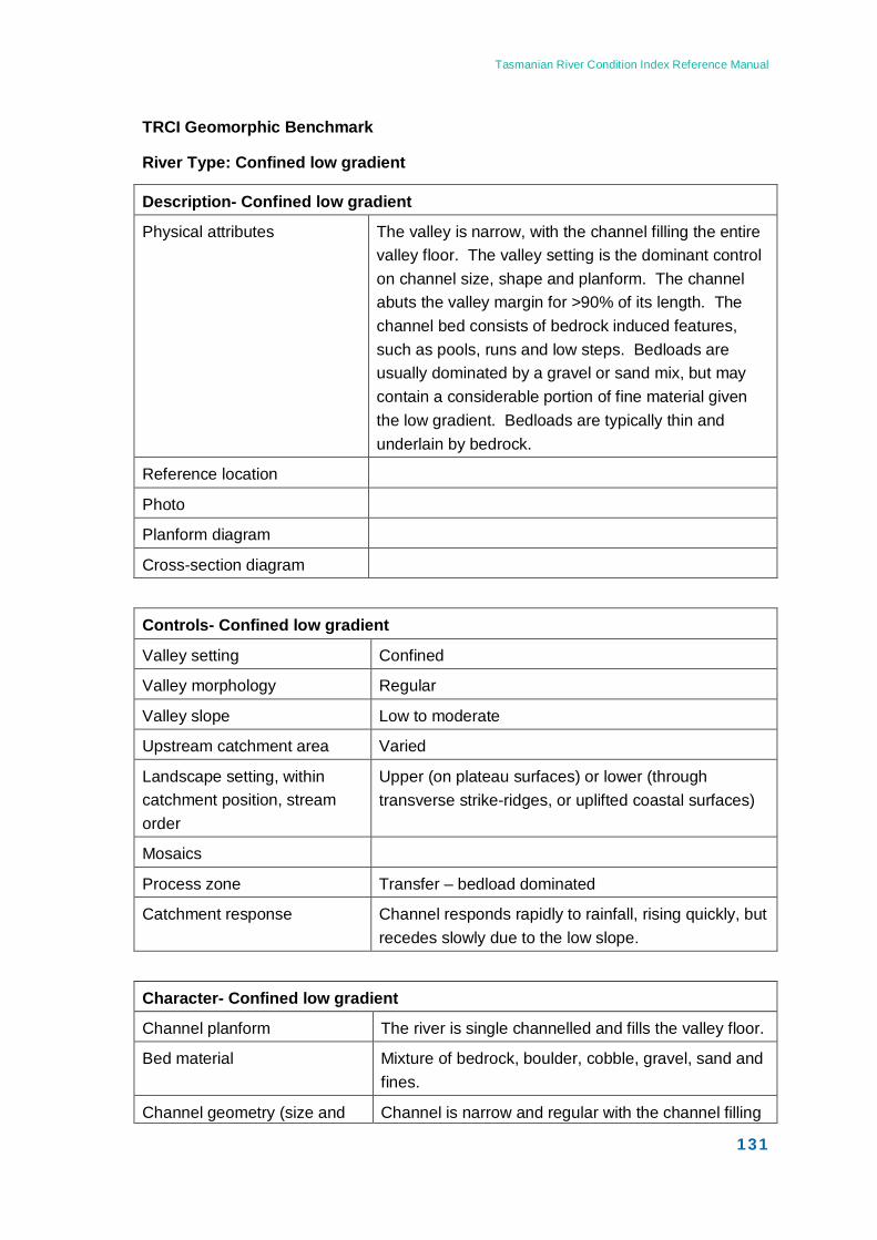
Tasmanian River Condition Index Reference Manual
131
TRCI Geomorphic Benchmark
River Type: Confined low gradient
Description- Confined low gradient
Physical attributes The valley is narrow, with the channel filling the entire valley floor. The valley setting is the dominant control on channel size, shape and planform. The channel abuts the valley margin for >90% of its length. The channel bed consists of bedrock induced features, such as pools, runs and low steps. Bedloads are usually dominated by a gravel or sand mix, but may contain a considerable portion of fine material given the low gradient. Bedloads are typically thin and underlain by bedrock.
Reference location
Photo
Planform diagram
Cross-section diagram
Controls- Confined low gradient
Valley setting Confined
Valley morphology Regular
Valley slope Low to moderate
Upstream catchment area Varied
Landscape setting, within catchment position, stream order
Upper (on plateau surfaces) or lower (through transverse strike-ridges, or uplifted coastal surfaces)
Mosaics
Process zone Transfer – bedload dominated
Catchment response Channel responds rapidly to rainfall, rising quickly, but recedes slowly due to the low slope.
Character- Confined low gradient
Channel planform The river is single channelled and fills the valley floor.
Bed material Mixture of bedrock, boulder, cobble, gravel, sand and fines.
Channel geometry (size and Channel is narrow and regular with the channel filling
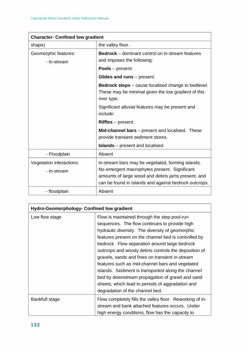
Tasmanian River Condition Index Reference Manual
132
Character- Confined low gradient shape) the valley floor.
Geomorphic features:
- In-stream
Bedrock – dominant control on in-stream features and imposes the following:
Pools – present.
Glides and runs – present.
Bedrock steps – cause localised change to bedlevel. These may be minimal given the low gradient of this river type.
Significant alluvial features may be present and include:
Riffles – present.
Mid-channel bars – present and localised. These provide transient sediment stores.
Islands – present and localised.
- Floodplain Absent
Vegetation interactions:
- In-stream
In-stream bars may be vegetated, forming islands. No emergent macrophytes present. Significant amounts of large wood and debris jams present, and can be found in islands and against bedrock outcrops.
- floodplain Absent
Hydro-Geomorphology- Confined low gradient
Low flow stage Flow is maintained through the step-pool-run sequences. The flow continues to provide high hydraulic diversity. The diversity of geomorphic features present on the channel bed is controlled by bedrock. Flow separation around large bedrock outcrops and woody debris controls the deposition of gravels, sands and fines on transient in-stream features such as mid-channel bars and vegetated islands. Sediment is transported along the channel bed by downstream propagation of gravel and sand sheets, which lead to periods of aggradation and degradation of the channel bed.
Bankfull stage Flow completely fills the valley floor. Reworking of in-stream and bank attached features occurs. Under high energy conditions, flow has the capacity to
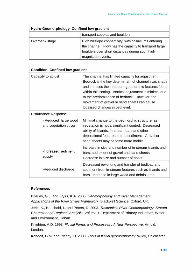
Tasmanian River Condition Index Reference Manual
133
Hydro-Geomorphology- Confined low gradient transport cobbles and boulders.
Overbank stage High hillslope connectivity, with colluviums entering the channel. Flow has the capacity to transport large boulders over short distances during such high magnitude events.
Condition- Confined low gradient
Capacity to adjust The channel has limited capacity for adjustment. Bedrock is the key determinant of channel size, shape and imposes the in-stream geomorphic features found within this setting. Vertical adjustment is minimal due to the predominance of bedrock. However, the movement of gravel or sand sheets can cause localised changes in bed level.
Disturbance Response
- Reduced large wood and vegetation cover
-Increased sediment supply
-Reduced discharge
Minimal change to the geomorphic structure, as vegetation is not a significant control. Decreased ability of islands, in-stream bars and other depositional features to trap sediment. Gravel or sand sheets may become more mobile.
Increase in size and number of in-stream islands and bars, and extent of gravel and sand sheets. Decrease in size and number of pools.
Decreased reworking and transfer of bedload and sediment from in-stream features such as islands and bars. Increase in large wood and debris jams.
References
Brierley, G.J. and Fryirs, K.A. 2005. Geomorphology and River Management: Applications of the River Styles Framework. Blackwell Science, Oxford, UK.
Jerie, K., Houshold, I., and Peters, D. 2003. Tasmania’s River Geomorphology: Stream Character and Regional Analysis, Volume 1. Department of Primary Industries, Water and Environment, Hobart.
Knighton, A.D. 1998. Fluvial Forms and Processes : A New Perspective. Arnold, London.
Kondolf, G.M. and Piegay, H. 2003. Tools in fluvial geomorphology. Wiley, Chichester.
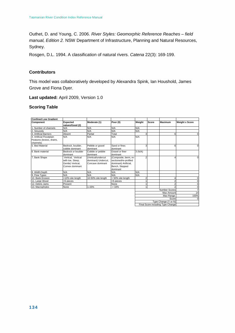
Tasmanian River Condition Index Reference Manual
134
Confined Low GradientComponent Expected
values/Good (2) Moderate (1) Poor (0) Weight Score Maximum Weight x Score
1. Number of channels N/A N/A N/A N/A2. Sinuosity N/A N/A N/A N/A3. Artificial Barriers Absent Partial Total 3 6 04. Artificial Floodplain Features (levees, drains, channels)
N/A N/A N/A N/A
5. Bed Material Bedrock, boulder, cobble dominant
Pebble or gravel dominant
Sand or fines dominant
3 6 0
6. Bank material Bedrock or boulder dominant
Cobble or pebble dominant
Gravel or finer dominant
3 (N/A)
7. Bank Shape Vertical, Vertical with toe, Steep, Gentle) Vertical, Convex dominant
(Vertical/undercut dominant) Undercut, Concave dominant
(Composite, berm, re-sectioned/re-profiled dominant) Artificial, Bench, Stepped dominant
2 4 0
8. Width:Depth N/A N/A N/A N/A9. Flow Types N/A N/A N/A N/A10. Bank Erosion <10% site length 10-50% site length > 50% site length 2 4 011. Large Wood >5 pieces <5 pieces 1 2 012. Debris Jams Present None 1 2 013. Macrophytes None 1-33% > 33% 1 2 0
Number Scores 7Max Amount 14Max Range 100%
Score 0Type Change (Y or N)
Final Score including Type Change
Outhet, D. and Young, C. 2006. River Styles: Geomorphic Reference Reaches – field manual, Edition 2. NSW Department of Infrastructure, Planning and Natural Resources, Sydney.
Rosgen, D.L. 1994. A classification of natural rivers. Catena 22(3): 169-199.
Contributors
This model was collaboratively developed by Alexandra Spink, Ian Houshold, James Grove and Fiona Dyer.
Last updated: April 2009, Version 1.0
Scoring Table
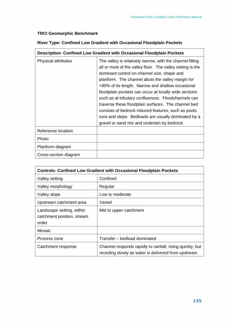
Tasmanian River Condition Index Reference Manual
135
TRCI Geomorphic Benchmark
River Type: Confined Low Gradient with Occasional Floodplain Pockets
Description- Confined Low Gradient with Occasional Floodplain Pockets
Physical attributes The valley is relatively narrow, with the channel filling all or most of the valley floor. The valley setting is the dominant control on channel size, shape and planform. The channel abuts the valley margin for >90% of its length. Narrow and shallow occasional floodplain pockets can occur at locally wide sections such as at tributary confluences. Floodchannels can traverse these floodplain surfaces. The channel bed consists of bedrock induced features, such as pools, runs and steps. Bedloads are usually dominated by a gravel or sand mix and underlain by bedrock.
Reference location
Photo
Planform diagram
Cross-section diagram
Controls- Confined Low Gradient with Occasional Floodplain Pockets
Valley setting Confined
Valley morphology Regular
Valley slope Low to moderate
Upstream catchment area Varied
Landscape setting, within catchment position, stream order
Mid to upper catchment
Mosaic
Process zone Transfer – bedload dominated
Catchment response Channel responds rapidly to rainfall, rising quickly, but receding slowly as water is delivered from upstream.
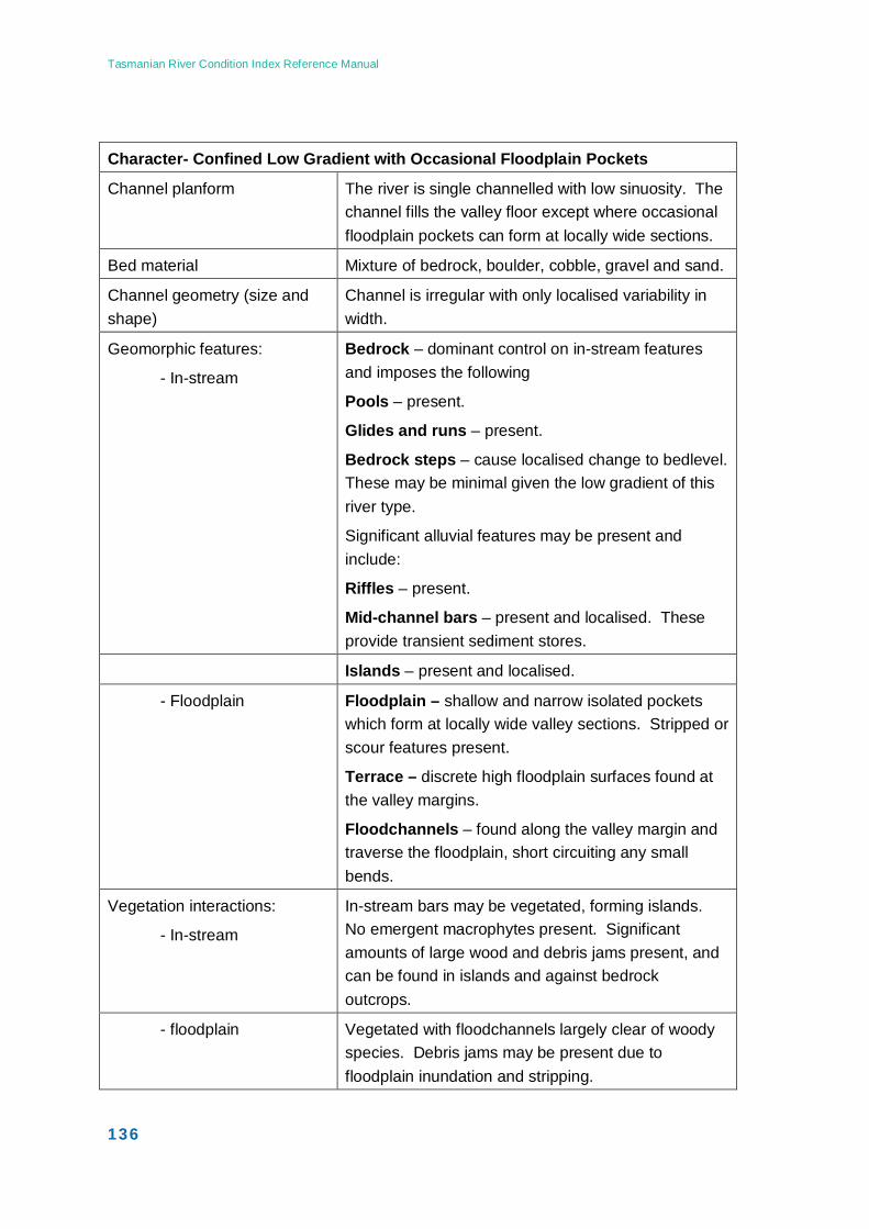
Tasmanian River Condition Index Reference Manual
136
Character- Confined Low Gradient with Occasional Floodplain Pockets
Channel planform The river is single channelled with low sinuosity. The channel fills the valley floor except where occasional floodplain pockets can form at locally wide sections.
Bed material Mixture of bedrock, boulder, cobble, gravel and sand.
Channel geometry (size and shape)
Channel is irregular with only localised variability in width.
Geomorphic features:
- In-stream
Bedrock – dominant control on in-stream features and imposes the following
Pools – present.
Glides and runs – present.
Bedrock steps – cause localised change to bedlevel. These may be minimal given the low gradient of this river type.
Significant alluvial features may be present and include:
Riffles – present.
Mid-channel bars – present and localised. These provide transient sediment stores.
Islands – present and localised.
- Floodplain Floodplain – shallow and narrow isolated pockets which form at locally wide valley sections. Stripped or scour features present.
Terrace – discrete high floodplain surfaces found at the valley margins.
Floodchannels – found along the valley margin and traverse the floodplain, short circuiting any small bends.
Vegetation interactions:
- In-stream
In-stream bars may be vegetated, forming islands. No emergent macrophytes present. Significant amounts of large wood and debris jams present, and can be found in islands and against bedrock outcrops.
- floodplain Vegetated with floodchannels largely clear of woody species. Debris jams may be present due to floodplain inundation and stripping.
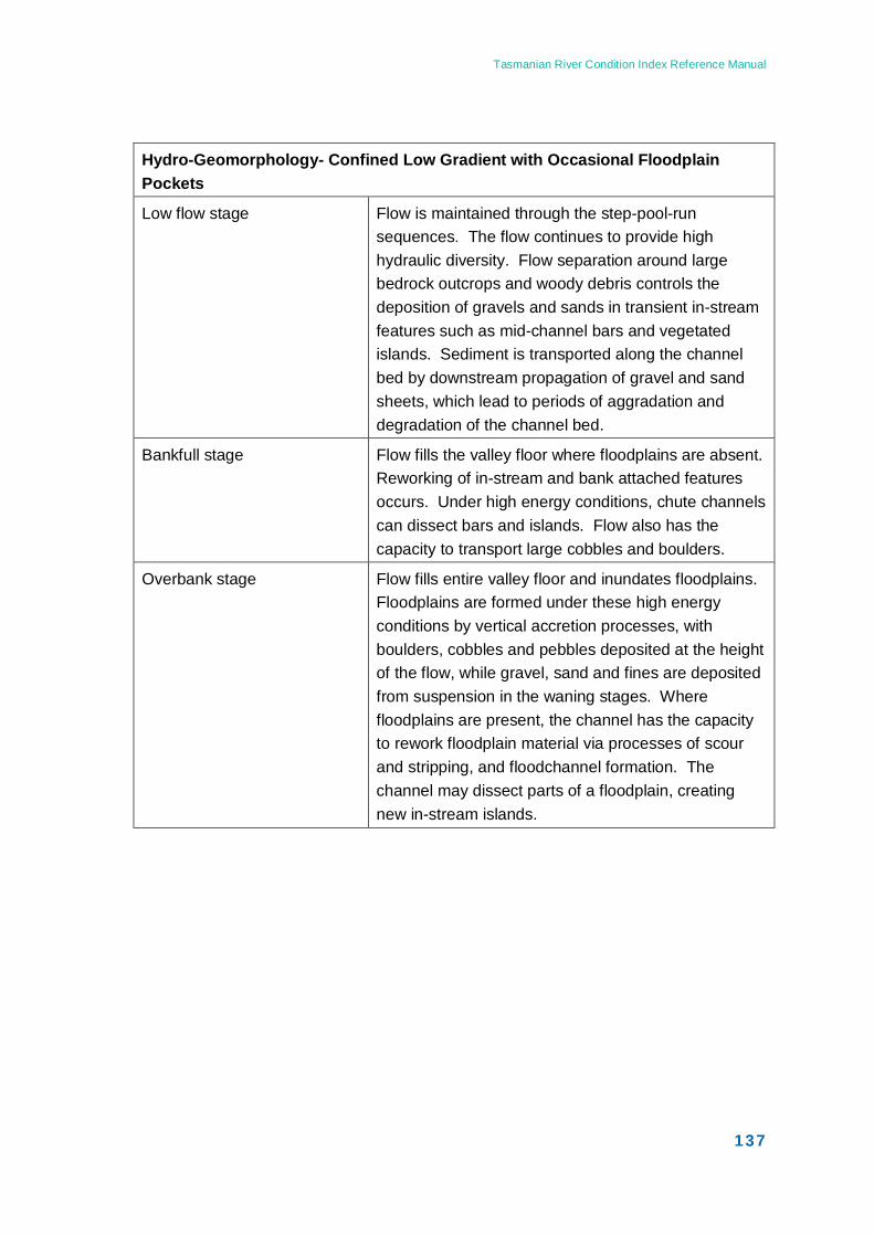
Tasmanian River Condition Index Reference Manual
137
Hydro-Geomorphology- Confined Low Gradient with Occasional Floodplain Pockets
Low flow stage Flow is maintained through the step-pool-run sequences. The flow continues to provide high hydraulic diversity. Flow separation around large bedrock outcrops and woody debris controls the deposition of gravels and sands in transient in-stream features such as mid-channel bars and vegetated islands. Sediment is transported along the channel bed by downstream propagation of gravel and sand sheets, which lead to periods of aggradation and degradation of the channel bed.
Bankfull stage Flow fills the valley floor where floodplains are absent. Reworking of in-stream and bank attached features occurs. Under high energy conditions, chute channels can dissect bars and islands. Flow also has the capacity to transport large cobbles and boulders.
Overbank stage Flow fills entire valley floor and inundates floodplains. Floodplains are formed under these high energy conditions by vertical accretion processes, with boulders, cobbles and pebbles deposited at the height of the flow, while gravel, sand and fines are deposited from suspension in the waning stages. Where floodplains are present, the channel has the capacity to rework floodplain material via processes of scour and stripping, and floodchannel formation. The channel may dissect parts of a floodplain, creating new in-stream islands.
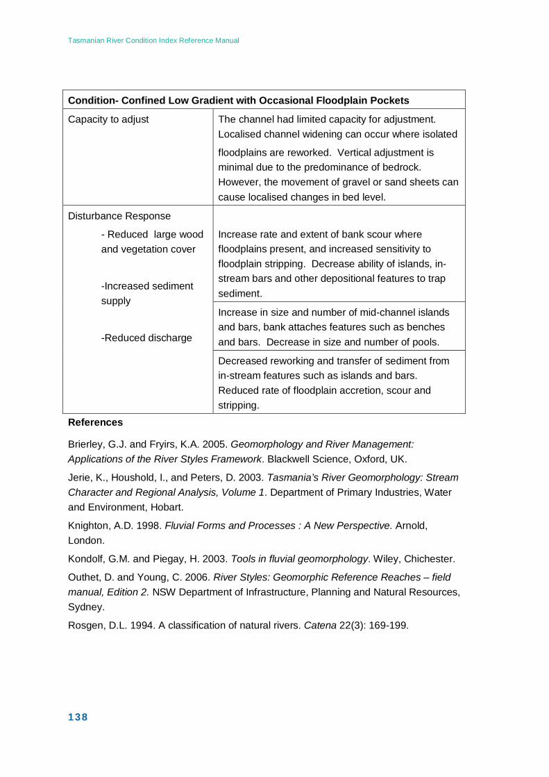
Tasmanian River Condition Index Reference Manual
138
Condition- Confined Low Gradient with Occasional Floodplain Pockets
Capacity to adjust
The channel had limited capacity for adjustment. Localised channel widening can occur where isolated
floodplains are reworked. Vertical adjustment is minimal due to the predominance of bedrock. However, the movement of gravel or sand sheets can cause localised changes in bed level.
Disturbance Response
- Reduced large wood and vegetation cover
-Increased sediment supply
-Reduced discharge
Increase rate and extent of bank scour where floodplains present, and increased sensitivity to floodplain stripping. Decrease ability of islands, in-stream bars and other depositional features to trap sediment.
Increase in size and number of mid-channel islands and bars, bank attaches features such as benches and bars. Decrease in size and number of pools.
Decreased reworking and transfer of sediment from in-stream features such as islands and bars. Reduced rate of floodplain accretion, scour and stripping.
References
Brierley, G.J. and Fryirs, K.A. 2005. Geomorphology and River Management: Applications of the River Styles Framework. Blackwell Science, Oxford, UK.
Jerie, K., Houshold, I., and Peters, D. 2003. Tasmania’s River Geomorphology: Stream Character and Regional Analysis, Volume 1. Department of Primary Industries, Water and Environment, Hobart.
Knighton, A.D. 1998. Fluvial Forms and Processes : A New Perspective. Arnold, London.
Kondolf, G.M. and Piegay, H. 2003. Tools in fluvial geomorphology. Wiley, Chichester.
Outhet, D. and Young, C. 2006. River Styles: Geomorphic Reference Reaches – field manual, Edition 2. NSW Department of Infrastructure, Planning and Natural Resources, Sydney.
Rosgen, D.L. 1994. A classification of natural rivers. Catena 22(3): 169-199.
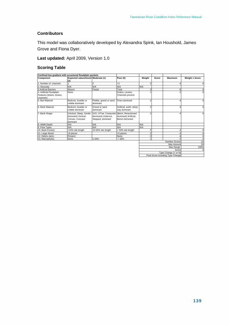
Tasmanian River Condition Index Reference Manual
139
Confined low gradient with occasional floodplain pockets Component Expected values/Good
(2)Moderate (1) Poor (0) Weight Score Maximum Weight x Score
1. Number of channels 1 2 >2 2 4 02. Sinuosity N/A N/A N/A N/A3.Artificial Barriers Absent Partial Total 3 6 04. Artificial Floodplain Features (drains, levees, channels)
None Drains, Levees, Channels present
1 2 0
5. Bed Material Bedrock, boulder or cobble dominant
Pebble, gravel or sand dominant
Fines dominant 2 4 0
6. Bank Material Bedrock, boulder or cobble dominant
Gravel or sand dominant
Artificial, earth, sticky clay dominant
2 4 0
7. Bank Shape (Vertical, Steep, Gentle dominant) Vertical, Convex, Concave dominant
(V/U, V/Toe, Composite dominant) Undercut, Stepped, dominant
(Berm, Resectioned dominant) Artificial, Bench dominant
2 4 0
8. Width:Depth N/A N/A N/A N/A9. Flow Types N/A N/A N/A N/A10. Bank Erosion <10% site length 10-50% site length > 50% site length 2 4 011. Large Wood >5 pieces <5 pieces 2 4 012. Debris Jams Present None 2 4 013. Macrophytes None 1-33% > 33% 1 2 0
Number Scores 10Max Amount 20Max Range 100%
Score 0Type Change (Y or N)
Final Score including Type Change
Contributors
This model was collaboratively developed by Alexandra Spink, Ian Houshold, James Grove and Fiona Dyer.
Last updated: April 2009, Version 1.0
Scoring Table
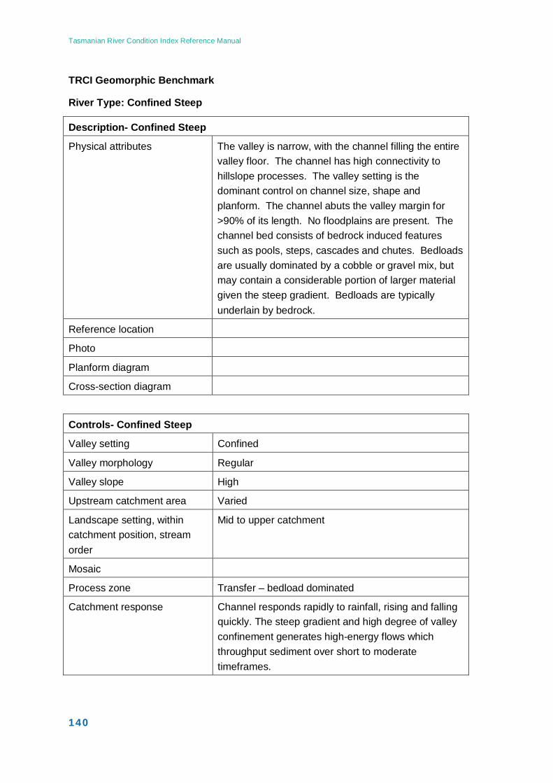
Tasmanian River Condition Index Reference Manual
140
TRCI Geomorphic Benchmark
River Type: Confined Steep
Description- Confined Steep
Physical attributes The valley is narrow, with the channel filling the entire valley floor. The channel has high connectivity to hillslope processes. The valley setting is the dominant control on channel size, shape and planform. The channel abuts the valley margin for >90% of its length. No floodplains are present. The channel bed consists of bedrock induced features such as pools, steps, cascades and chutes. Bedloads are usually dominated by a cobble or gravel mix, but may contain a considerable portion of larger material given the steep gradient. Bedloads are typically underlain by bedrock.
Reference location
Photo
Planform diagram
Cross-section diagram
Controls- Confined Steep
Valley setting Confined
Valley morphology Regular
Valley slope High
Upstream catchment area Varied
Landscape setting, within catchment position, stream order
Mid to upper catchment
Mosaic
Process zone Transfer – bedload dominated
Catchment response Channel responds rapidly to rainfall, rising and falling quickly. The steep gradient and high degree of valley confinement generates high-energy flows which throughput sediment over short to moderate timeframes.
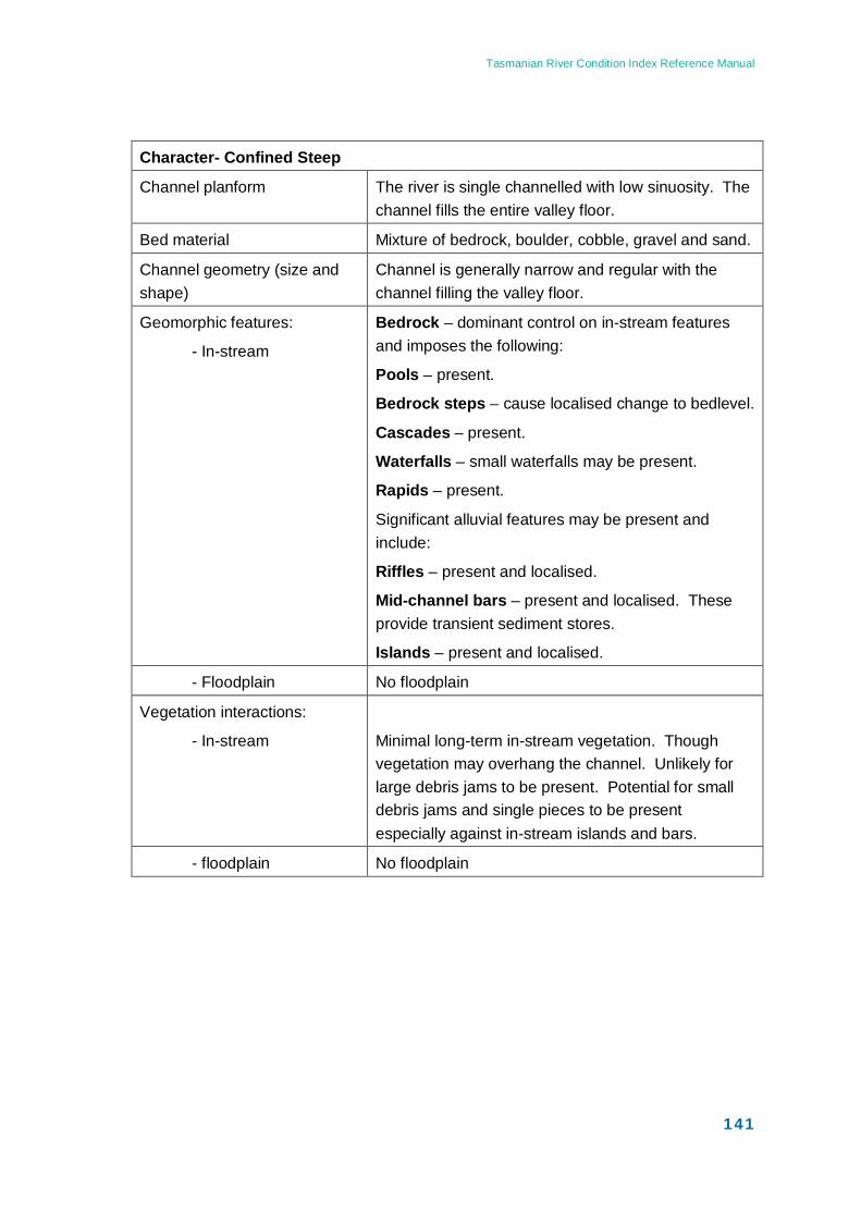
Tasmanian River Condition Index Reference Manual
141
Character- Confined Steep
Channel planform The river is single channelled with low sinuosity. The channel fills the entire valley floor.
Bed material Mixture of bedrock, boulder, cobble, gravel and sand.
Channel geometry (size and shape)
Channel is generally narrow and regular with the channel filling the valley floor.
Geomorphic features:
- In-stream
Bedrock – dominant control on in-stream features and imposes the following:
Pools – present.
Bedrock steps – cause localised change to bedlevel.
Cascades – present.
Waterfalls – small waterfalls may be present.
Rapids – present.
Significant alluvial features may be present and include:
Riffles – present and localised.
Mid-channel bars – present and localised. These provide transient sediment stores.
Islands – present and localised.
- Floodplain No floodplain
Vegetation interactions:
- In-stream
Minimal long-term in-stream vegetation. Though vegetation may overhang the channel. Unlikely for large debris jams to be present. Potential for small debris jams and single pieces to be present especially against in-stream islands and bars.
- floodplain No floodplain
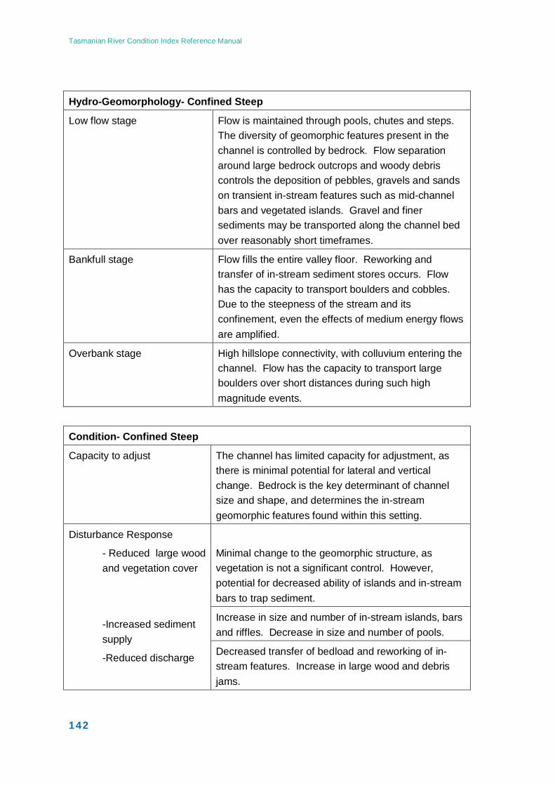
Tasmanian River Condition Index Reference Manual
142
Hydro-Geomorphology- Confined Steep
Low flow stage Flow is maintained through pools, chutes and steps. The diversity of geomorphic features present in the channel is controlled by bedrock. Flow separation around large bedrock outcrops and woody debris controls the deposition of pebbles, gravels and sands on transient in-stream features such as mid-channel bars and vegetated islands. Gravel and finer sediments may be transported along the channel bed over reasonably short timeframes.
Bankfull stage Flow fills the entire valley floor. Reworking and transfer of in-stream sediment stores occurs. Flow has the capacity to transport boulders and cobbles. Due to the steepness of the stream and its confinement, even the effects of medium energy flows are amplified.
Overbank stage High hillslope connectivity, with colluvium entering the channel. Flow has the capacity to transport large boulders over short distances during such high magnitude events.
Condition- Confined Steep
Capacity to adjust The channel has limited capacity for adjustment, as there is minimal potential for lateral and vertical change. Bedrock is the key determinant of channel size and shape, and determines the in-stream geomorphic features found within this setting.
Disturbance Response
- Reduced large wood and vegetation cover
-Increased sediment supply
-Reduced discharge
Minimal change to the geomorphic structure, as vegetation is not a significant control. However, potential for decreased ability of islands and in-stream bars to trap sediment.
Increase in size and number of in-stream islands, bars and riffles. Decrease in size and number of pools.
Decreased transfer of bedload and reworking of in-stream features. Increase in large wood and debris jams.
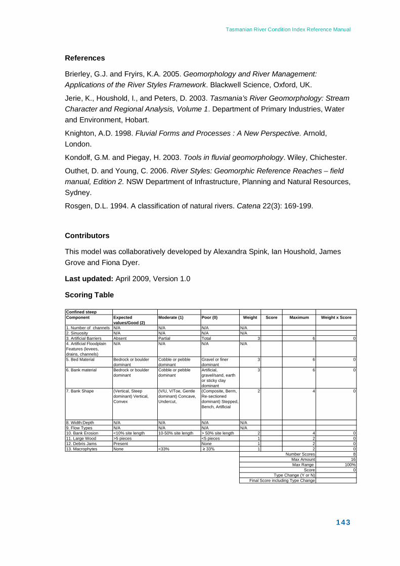
Tasmanian River Condition Index Reference Manual
143
Confined steepComponent Expected
values/Good (2)Moderate (1) Poor (0) Weight Score Maximum Weight x Score
1. Number of channels N/A N/A N/A N/A2. Sinuosity N/A N/A N/A N/A3. Artificial Barriers Absent Partial Total 3 6 04. Artificial Floodplain Features (levees, drains, channels)
N/A N/A N/A N/A
5. Bed Material Bedrock or boulder dominant
Cobble or pebble dominant
Gravel or finer dominant
3 6 0
6. Bank material Bedrock or boulder dominant
Cobble or pebble dominant
Artificial, gravel/sand, earth or sticky clay dominant
3 6 0
7. Bank Shape (Vertical, Steep dominant) Vertical, Convex
(V/U, V/Toe, Gentle dominant) Concave, Undercut,
(Composite, Berm, Re-sectioned dominant) Stepped, Bench, Artificial
2 4 0
8. Width:Depth N/A N/A N/A N/A9. Flow Types N/A N/A N/A N/A10. Bank Erosion <10% site length 10-50% site length > 50% site length 2 4 011. Large Wood >5 pieces <5 pieces 1 2 012. Debris Jams Present None 1 2 013. Macrophytes None <33% ≥ 33% 1 2 0
Number Scores 8Max Amount 16Max Range 100%
Score 0Type Change (Y or N)
Final Score including Type Change
References
Brierley, G.J. and Fryirs, K.A. 2005. Geomorphology and River Management: Applications of the River Styles Framework. Blackwell Science, Oxford, UK.
Jerie, K., Houshold, I., and Peters, D. 2003. Tasmania’s River Geomorphology: Stream Character and Regional Analysis, Volume 1. Department of Primary Industries, Water and Environment, Hobart.
Knighton, A.D. 1998. Fluvial Forms and Processes : A New Perspective. Arnold, London.
Kondolf, G.M. and Piegay, H. 2003. Tools in fluvial geomorphology. Wiley, Chichester.
Outhet, D. and Young, C. 2006. River Styles: Geomorphic Reference Reaches – field manual, Edition 2. NSW Department of Infrastructure, Planning and Natural Resources, Sydney.
Rosgen, D.L. 1994. A classification of natural rivers. Catena 22(3): 169-199.
Contributors
This model was collaboratively developed by Alexandra Spink, Ian Houshold, James Grove and Fiona Dyer.
Last updated: April 2009, Version 1.0
Scoring Table
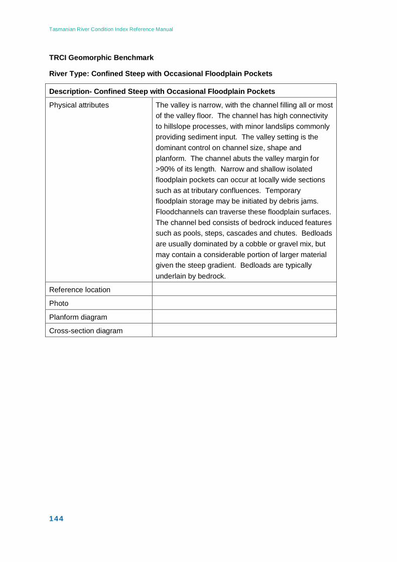
Tasmanian River Condition Index Reference Manual
144
TRCI Geomorphic Benchmark
River Type: Confined Steep with Occasional Floodplain Pockets
Description- Confined Steep with Occasional Floodplain Pockets
Physical attributes The valley is narrow, with the channel filling all or most of the valley floor. The channel has high connectivity to hillslope processes, with minor landslips commonly providing sediment input. The valley setting is the dominant control on channel size, shape and planform. The channel abuts the valley margin for >90% of its length. Narrow and shallow isolated floodplain pockets can occur at locally wide sections such as at tributary confluences. Temporary floodplain storage may be initiated by debris jams. Floodchannels can traverse these floodplain surfaces. The channel bed consists of bedrock induced features such as pools, steps, cascades and chutes. Bedloads are usually dominated by a cobble or gravel mix, but may contain a considerable portion of larger material given the steep gradient. Bedloads are typically underlain by bedrock.
Reference location
Photo
Planform diagram
Cross-section diagram
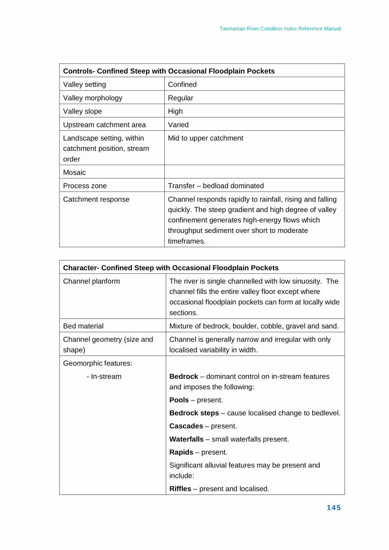
Tasmanian River Condition Index Reference Manual
145
Controls- Confined Steep with Occasional Floodplain Pockets
Valley setting Confined
Valley morphology Regular
Valley slope High
Upstream catchment area Varied
Landscape setting, within catchment position, stream order
Mid to upper catchment
Mosaic
Process zone Transfer – bedload dominated
Catchment response Channel responds rapidly to rainfall, rising and falling quickly. The steep gradient and high degree of valley confinement generates high-energy flows which throughput sediment over short to moderate timeframes.
Character- Confined Steep with Occasional Floodplain Pockets
Channel planform The river is single channelled with low sinuosity. The channel fills the entire valley floor except where occasional floodplain pockets can form at locally wide sections.
Bed material Mixture of bedrock, boulder, cobble, gravel and sand.
Channel geometry (size and shape)
Channel is generally narrow and irregular with only localised variability in width.
Geomorphic features:
- In-stream
Bedrock – dominant control on in-stream features and imposes the following:
Pools – present.
Bedrock steps – cause localised change to bedlevel.
Cascades – present.
Waterfalls – small waterfalls present.
Rapids – present.
Significant alluvial features may be present and include:
Riffles – present and localised.
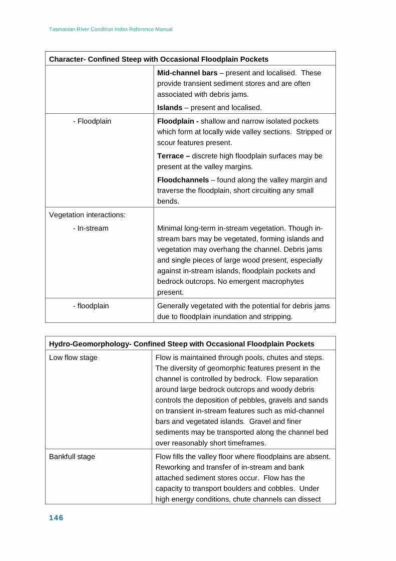
Tasmanian River Condition Index Reference Manual
146
Character- Confined Steep with Occasional Floodplain Pockets
Mid-channel bars – present and localised. These provide transient sediment stores and are often associated with debris jams.
Islands – present and localised.
- Floodplain Floodplain - shallow and narrow isolated pockets which form at locally wide valley sections. Stripped or scour features present.
Terrace – discrete high floodplain surfaces may be present at the valley margins.
Floodchannels – found along the valley margin and traverse the floodplain, short circuiting any small bends.
Vegetation interactions:
- In-stream
Minimal long-term in-stream vegetation. Though in-stream bars may be vegetated, forming islands and vegetation may overhang the channel. Debris jams and single pieces of large wood present, especially against in-stream islands, floodplain pockets and bedrock outcrops. No emergent macrophytes present.
- floodplain Generally vegetated with the potential for debris jams due to floodplain inundation and stripping.
Hydro-Geomorphology- Confined Steep with Occasional Floodplain Pockets
Low flow stage Flow is maintained through pools, chutes and steps. The diversity of geomorphic features present in the channel is controlled by bedrock. Flow separation around large bedrock outcrops and woody debris controls the deposition of pebbles, gravels and sands on transient in-stream features such as mid-channel bars and vegetated islands. Gravel and finer sediments may be transported along the channel bed over reasonably short timeframes.
Bankfull stage Flow fills the valley floor where floodplains are absent. Reworking and transfer of in-stream and bank attached sediment stores occur. Flow has the capacity to transport boulders and cobbles. Under high energy conditions, chute channels can dissect
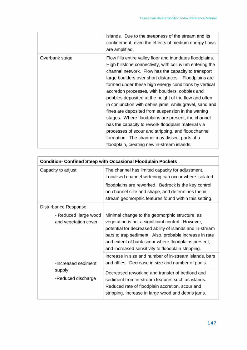
Tasmanian River Condition Index Reference Manual
147
islands. Due to the steepness of the stream and its confinement, even the effects of medium energy flows are amplified.
Overbank stage Flow fills entire valley floor and inundates floodplains. High hillslope connectivity, with colluvium entering the channel network. Flow has the capacity to transport large boulders over short distances. Floodplains are formed under these high energy conditions by vertical accretion processes, with boulders, cobbles and pebbles deposited at the height of the flow and often in conjunction with debris jams; while gravel, sand and fines are deposited from suspension in the waning stages. Where floodplains are present, the channel has the capacity to rework floodplain material via processes of scour and stripping, and floodchannel formation. The channel may dissect parts of a floodplain, creating new in-stream islands.
Condition- Confined Steep with Occasional Floodplain Pockets
Capacity to adjust The channel has limited capacity for adjustment. Localised channel widening can occur where isolated
floodplains are reworked. Bedrock is the key control on channel size and shape, and determines the in-stream geomorphic features found within this setting.
Disturbance Response
- Reduced large wood and vegetation cover
-Increased sediment supply
-Reduced discharge
Minimal change to the geomorphic structure, as vegetation is not a significant control. However, potential for decreased ability of islands and in-stream bars to trap sediment. Also, probable increase in rate and extent of bank scour where floodplains present, and increased sensitivity to floodplain stripping. Increase in size and number of in-stream islands, bars and riffles. Decrease in size and number of pools.
Decreased reworking and transfer of bedload and sediment from in-stream features such as islands. Reduced rate of floodplain accretion, scour and stripping. Increase in large wood and debris jams.
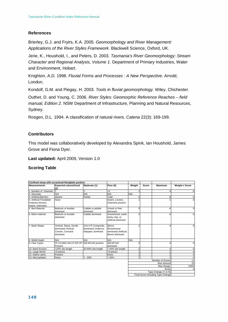
Tasmanian River Condition Index Reference Manual
148
Confined steep with occasional floodplain pockets Measurements Expected values/Good
(2)Moderate (1) Poor (0) Weight Score Maximum Weight x Score
1. Number of channels 1 2 >2 2 4 02. Sinuosity N/A N/A N/A N/A3. Artificial Barriers Absent Partial Total 3 6 04. Artificial Floodplain Features (levees, drains, channels)
None Drains, Levees, Channels present
1 2 0
5. Bed Material Bedrock or boulder dominant
Cobble or pebble dominant
Gravel or finer dominant
3 6 0
6. Bank material Bedrock or boulder dominant
Cobble dominant Gravel/sand, earth, sticky clay, or artificial dominant
3 6 0
7. Bank Shape Vertical, Steep, Gentle dominant) Vertical, Convex, Concave dominant
(V/U,V/T,Composite, dominant) Undercut, Stepped, dominant
(Berm, Resectioned dominant) Artificial, Bench dominant
2 4 0
8. Width:Depth N/A N/A N/A N/A9. Flow Types FF,CH,BW,UW,CF,RP,UP
PresentSM,NP,NO present SM,NP,NO
dominant2 4 0
10. Bank Erosion <20% site length 20-50% site length > 50% site length 2 4 011. Large Wood >5 pieces <5 pieces 1 2 012. Debris Jams Present None 1 2 013. Macrophytes None 1 - 33% >33% 1 2 0
Number of Scores 11Max Amount 22Max Range 100%
Score 0Type Change (Y or N)
Final Score including Type Change
References
Brierley, G.J. and Fryirs, K.A. 2005. Geomorphology and River Management: Applications of the River Styles Framework. Blackwell Science, Oxford, UK.
Jerie, K., Houshold, I., and Peters, D. 2003. Tasmania’s River Geomorphology: Stream Character and Regional Analysis, Volume 1. Department of Primary Industries, Water and Environment, Hobart.
Knighton, A.D. 1998. Fluvial Forms and Processes : A New Perspective. Arnold, London.
Kondolf, G.M. and Piegay, H. 2003. Tools in fluvial geomorphology. Wiley, Chichester.
Outhet, D. and Young, C. 2006. River Styles: Geomorphic Reference Reaches – field manual, Edition 2. NSW Department of Infrastructure, Planning and Natural Resources, Sydney.
Rosgen, D.L. 1994. A classification of natural rivers. Catena 22(3): 169-199.
Contributors
This model was collaboratively developed by Alexandra Spink, Ian Houshold, James Grove and Fiona Dyer.
Last updated: April 2009, Version 1.0
Scoring Table
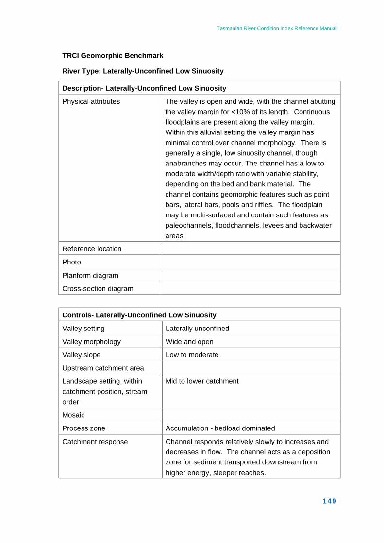
Tasmanian River Condition Index Reference Manual
149
TRCI Geomorphic Benchmark
River Type: Laterally-Unconfined Low Sinuosity
Description- Laterally-Unconfined Low Sinuosity
Physical attributes The valley is open and wide, with the channel abutting the valley margin for <10% of its length. Continuous floodplains are present along the valley margin. Within this alluvial setting the valley margin has minimal control over channel morphology. There is generally a single, low sinuosity channel, though anabranches may occur. The channel has a low to moderate width/depth ratio with variable stability, depending on the bed and bank material. The channel contains geomorphic features such as point bars, lateral bars, pools and riffles. The floodplain may be multi-surfaced and contain such features as paleochannels, floodchannels, levees and backwater areas.
Reference location
Photo
Planform diagram
Cross-section diagram
Controls- Laterally-Unconfined Low Sinuosity
Valley setting Laterally unconfined
Valley morphology Wide and open
Valley slope Low to moderate
Upstream catchment area
Landscape setting, within catchment position, stream order
Mid to lower catchment
Mosaic
Process zone Accumulation - bedload dominated
Catchment response Channel responds relatively slowly to increases and decreases in flow. The channel acts as a deposition zone for sediment transported downstream from higher energy, steeper reaches.
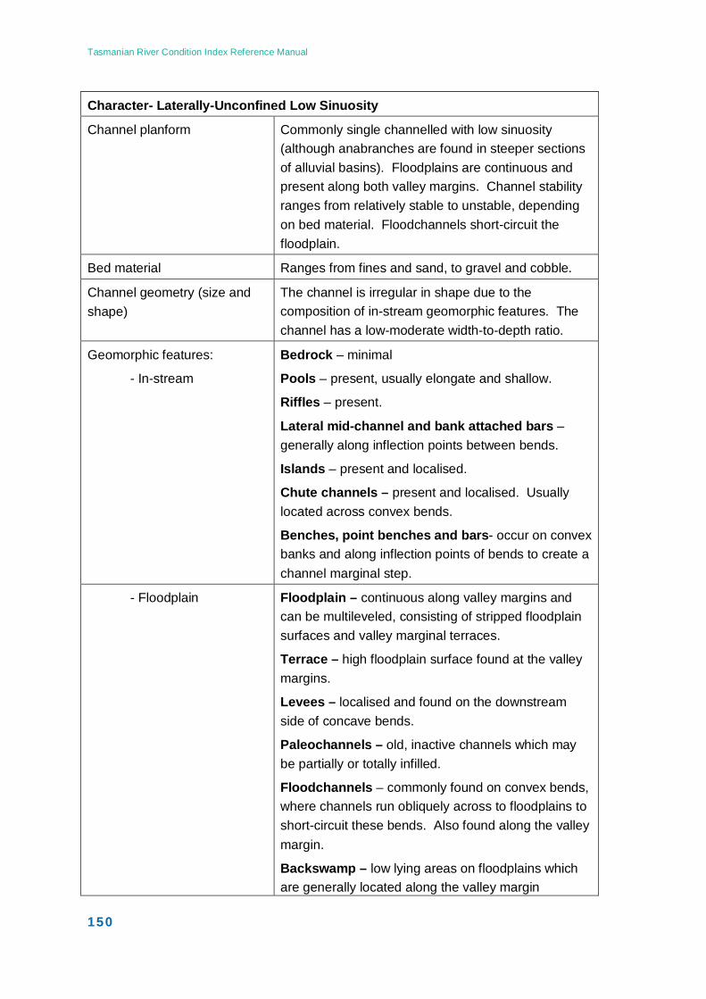
Tasmanian River Condition Index Reference Manual
150
Character- Laterally-Unconfined Low Sinuosity
Channel planform Commonly single channelled with low sinuosity (although anabranches are found in steeper sections of alluvial basins). Floodplains are continuous and present along both valley margins. Channel stability ranges from relatively stable to unstable, depending on bed material. Floodchannels short-circuit the floodplain.
Bed material Ranges from fines and sand, to gravel and cobble.
Channel geometry (size and shape)
The channel is irregular in shape due to the composition of in-stream geomorphic features. The channel has a low-moderate width-to-depth ratio.
Geomorphic features:
- In-stream
Bedrock – minimal
Pools – present, usually elongate and shallow.
Riffles – present.
Lateral mid-channel and bank attached bars – generally along inflection points between bends.
Islands – present and localised.
Chute channels – present and localised. Usually located across convex bends.
Benches, point benches and bars- occur on convex banks and along inflection points of bends to create a channel marginal step.
- Floodplain Floodplain – continuous along valley margins and can be multileveled, consisting of stripped floodplain surfaces and valley marginal terraces.
Terrace – high floodplain surface found at the valley margins.
Levees – localised and found on the downstream side of concave bends.
Paleochannels – old, inactive channels which may be partially or totally infilled.
Floodchannels – commonly found on convex bends, where channels run obliquely across to floodplains to short-circuit these bends. Also found along the valley margin.
Backswamp – low lying areas on floodplains which are generally located along the valley margin
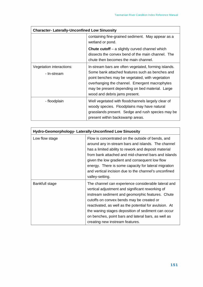
Tasmanian River Condition Index Reference Manual
151
Character- Laterally-Unconfined Low Sinuosity containing fine-grained sediment. May appear as a wetland or pond.
Chute cutoff – a slightly curved channel which dissects the convex bend of the main channel. The chute then becomes the main channel.
Vegetation interactions:
- In-stream
In-stream bars are often vegetated, forming islands. Some bank attached features such as benches and point benches may be vegetated, with vegetation overhanging the channel. Emergent macrophytes may be present depending on bed material. Large wood and debris jams present.
- floodplain Well vegetated with floodchannels largely clear of woody species. Floodplains may have natural grasslands present. Sedge and rush species may be present within backswamp areas.
Hydro-Geomorphology- Laterally-Unconfined Low Sinuosity
Low flow stage Flow is concentrated on the outside of bends, and around any in-stream bars and islands. The channel has a limited ability to rework and deposit material from bank attached and mid-channel bars and islands given the low gradient and consequent low flow energy. There is some capacity for lateral migration and vertical incision due to the channel’s unconfined valley-setting.
Bankfull stage The channel can experience considerable lateral and vertical adjustment and significant reworking of instream sediment and geomorphic features. Chute cutoffs on convex bends may be created or reactivated, as well as the potential for avulsion. At the waning stages deposition of sediment can occur on benches, point bars and lateral bars, as well as creating new instream features.
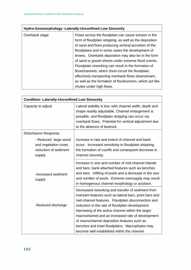
Tasmanian River Condition Index Reference Manual
152
Hydro-Geomorphology- Laterally-Unconfined Low Sinuosity
Overbank stage Flows across the floodplain can cause erosion in the form of floodplain stripping, as well as the deposition of sand and fines producing vertical accretion of the floodplains and in some cases the development of levees. Overbank deposition may also be in the form of sand or gravel sheets under extreme flood events. Floodplain reworking can result in the formation of floodchannels, which short-circuit the floodplain, effectively transporting overbank flows downstream, as well as the formation of floodrunners, which act like chutes under high flows.
Condition- Laterally-Unconfined Low Sinuosity
Capacity to adjust Lateral stability is low, with channel width, depth and shape readily adjustable. Channel enlargement is possible, and floodplain stripping can occur via overbank flows. Potential for vertical adjustment due to the absence of bedrock.
Disturbance Response
- Reduced large wood and vegetation cover, reduction of sediment supply
-Increased sediment supply
-Reduced discharge
Increase in rate and extent of channel and bank scour. Increased sensitivity to floodplain stripping, the formation of cutoffs and consequent decrease in channel sinuosity.
Increase in size and number of mid-channel islands and bars, bank attached features such as benches and bars. Infilling of pools and a decrease in the size and number of pools. Extreme oversupply may result in homogenous channel morphology or avulsion.
Decreased reworking and transfer of sediment from instream features such as lateral bars, point bars and mid-channel features. Floodplain disconnection and reduction in the rate of floodplain development. Narrowing of the active channel within the larger macrochannel and an increased rate of development of macrochannel deposition features such as benches and inset floodplains. Macrophytes may become well established within the channel.
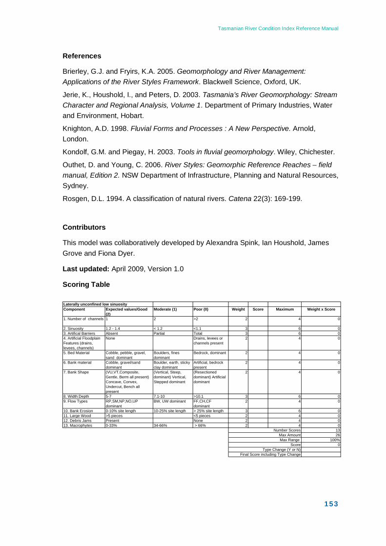
Tasmanian River Condition Index Reference Manual
153
Laterally unconfined low sinuosityComponent Expected values/Good
(2)Moderate (1) Poor (0) Weight Score Maximum Weight x Score
1. Number of channels 1 2 >2 2 4 0
2. Sinuosity 1.2 - 1.4 < 1.2 <1.1 3 6 03. Artifical Barriers Absent Partial Total 3 6 04. Artificial Floodplain Features (drains, levees, channels)
None Drains, levees or channels present
2 4 0
5. Bed Material Cobble, pebble, gravel, sand dominant
Boulders, fines dominant
Bedrock, dominant 2 4 0
6. Bank material Cobble, gravel/sand dominant
Boulder, earth, sticky clay dominant
Artificial, bedrock present
2 4 0
7. Bank Shape (VU,VT,Composite, Gentle, Berm all present) Concave, Convex, Undercut, Bench all present
(Vertical, Steep, dominant) Vertical, Stepped dominant
(Resectioned dominant) Artificial dominant
2 4 0
8. Width:Depth 5-7 7.1-10 >10.1 3 6 09. Flow Types RP,SM,NP,NO,UP
dominantBW, UW dominant FF,CH,CF
dominant2 4 0
10. Bank Erosion 0-10% site length 10-25% site length > 25% site length 3 6 011. Large Wood >5 pieces <5 pieces 2 4 012. Debris Jams Present None 2 4 013. Macrophytes 0-33% 34-66% > 66% 2 4 0
Number Scores 13Max Amount 26Max Range 100%
Score 0Type Change (Y or N)
Final Score including Type Change
References
Brierley, G.J. and Fryirs, K.A. 2005. Geomorphology and River Management: Applications of the River Styles Framework. Blackwell Science, Oxford, UK.
Jerie, K., Houshold, I., and Peters, D. 2003. Tasmania’s River Geomorphology: Stream Character and Regional Analysis, Volume 1. Department of Primary Industries, Water and Environment, Hobart.
Knighton, A.D. 1998. Fluvial Forms and Processes : A New Perspective. Arnold, London.
Kondolf, G.M. and Piegay, H. 2003. Tools in fluvial geomorphology. Wiley, Chichester.
Outhet, D. and Young, C. 2006. River Styles: Geomorphic Reference Reaches – field manual, Edition 2. NSW Department of Infrastructure, Planning and Natural Resources, Sydney.
Rosgen, D.L. 1994. A classification of natural rivers. Catena 22(3): 169-199.
Contributors
This model was collaboratively developed by Alexandra Spink, Ian Houshold, James Grove and Fiona Dyer.
Last updated: April 2009, Version 1.0
Scoring Table
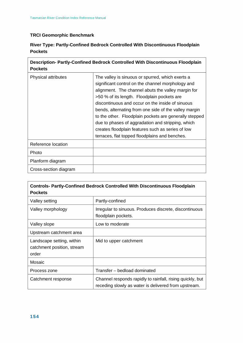
Tasmanian River Condition Index Reference Manual
154
TRCI Geomorphic Benchmark
River Type: Partly-Confined Bedrock Controlled With Discontinuous Floodplain Pockets
Description- Partly-Confined Bedrock Controlled With Discontinuous Floodplain Pockets
Physical attributes The valley is sinuous or spurred, which exerts a significant control on the channel morphology and alignment. The channel abuts the valley margin for >50 % of its length. Floodplain pockets are discontinuous and occur on the inside of sinuous bends, alternating from one side of the valley margin to the other. Floodplain pockets are generally stepped due to phases of aggradation and stripping, which creates floodplain features such as series of low terraces, flat topped floodplains and benches.
Reference location
Photo
Planform diagram
Cross-section diagram
Controls- Partly-Confined Bedrock Controlled With Discontinuous Floodplain Pockets
Valley setting Partly-confined
Valley morphology Irregular to sinuous. Produces discrete, discontinuous floodplain pockets.
Valley slope Low to moderate
Upstream catchment area
Landscape setting, within catchment position, stream order
Mid to upper catchment
Mosaic
Process zone Transfer – bedload dominated
Catchment response Channel responds rapidly to rainfall, rising quickly, but receding slowly as water is delivered from upstream.
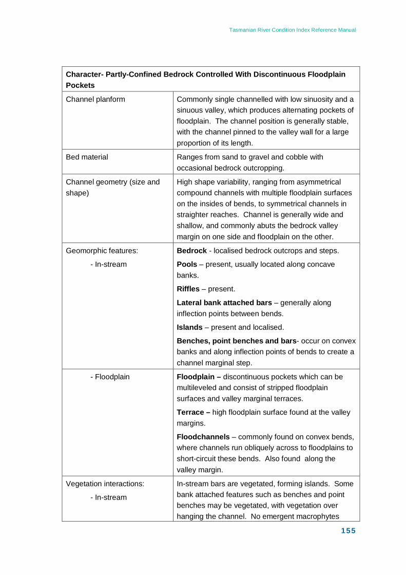
Tasmanian River Condition Index Reference Manual
155
Character- Partly-Confined Bedrock Controlled With Discontinuous Floodplain Pockets
Channel planform Commonly single channelled with low sinuosity and a sinuous valley, which produces alternating pockets of floodplain. The channel position is generally stable, with the channel pinned to the valley wall for a large proportion of its length.
Bed material Ranges from sand to gravel and cobble with occasional bedrock outcropping.
Channel geometry (size and shape)
High shape variability, ranging from asymmetrical compound channels with multiple floodplain surfaces on the insides of bends, to symmetrical channels in straighter reaches. Channel is generally wide and shallow, and commonly abuts the bedrock valley margin on one side and floodplain on the other.
Geomorphic features:
- In-stream
Bedrock - localised bedrock outcrops and steps.
Pools – present, usually located along concave banks.
Riffles – present.
Lateral bank attached bars – generally along inflection points between bends.
Islands – present and localised.
Benches, point benches and bars- occur on convex banks and along inflection points of bends to create a channel marginal step.
- Floodplain Floodplain – discontinuous pockets which can be multileveled and consist of stripped floodplain surfaces and valley marginal terraces.
Terrace – high floodplain surface found at the valley margins.
Floodchannels – commonly found on convex bends, where channels run obliquely across to floodplains to short-circuit these bends. Also found along the valley margin.
Vegetation interactions:
- In-stream
In-stream bars are vegetated, forming islands. Some bank attached features such as benches and point benches may be vegetated, with vegetation over hanging the channel. No emergent macrophytes
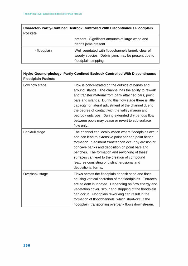
Tasmanian River Condition Index Reference Manual
156
Character- Partly-Confined Bedrock Controlled With Discontinuous Floodplain Pockets
present. Significant amounts of large wood and debris jams present.
- floodplain Well vegetated with floodchannels largely clear of woody species. Debris jams may be present due to floodplain stripping.
Hydro-Geomorphology- Partly-Confined Bedrock Controlled With Discontinuous Floodplain Pockets
Low flow stage Flow is concentrated on the outside of bends and around islands. The channel has the ability to rework and transfer material from bank attached bars, point bars and islands. During this flow stage there is little capacity for lateral adjustment of the channel due to the degree of contact with the valley margin and bedrock outcrops. During extended dry periods flow between pools may cease or revert to sub-surface flow only.
Bankfull stage The channel can locally widen where floodplains occur and can lead to extensive point bar and point bench formation. Sediment transfer can occur by erosion of concave banks and deposition on point bars and benches. The formation and reworking of these surfaces can lead to the creation of compound features consisting of distinct erosional and depositional forms.
Overbank stage Flows across the floodplain deposit sand and fines causing vertical accretion of the floodplains. Terraces are seldom inundated. Depending on flow energy and vegetation cover, scour and stripping of the floodplain can occur. Floodplain reworking can result in the formation of floodchannels, which short-circuit the floodplain, transporting overbank flows downstream.
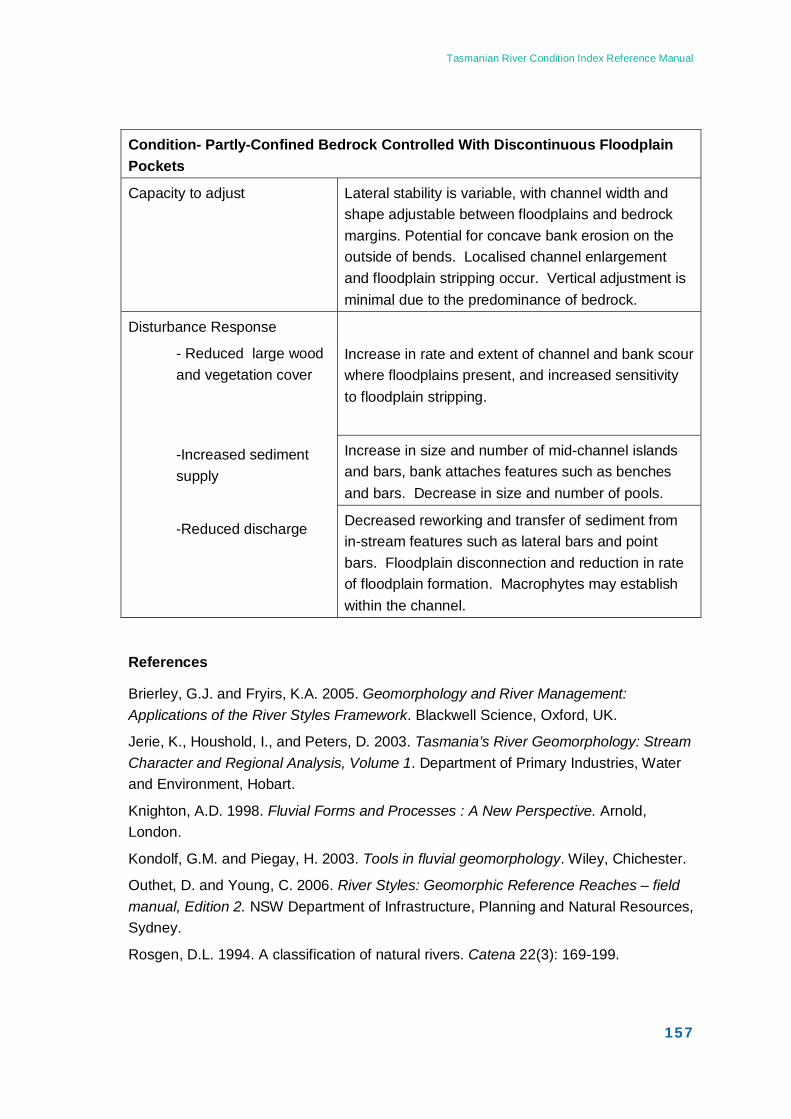
Tasmanian River Condition Index Reference Manual
157
Condition- Partly-Confined Bedrock Controlled With Discontinuous Floodplain Pockets
Capacity to adjust Lateral stability is variable, with channel width and shape adjustable between floodplains and bedrock margins. Potential for concave bank erosion on the outside of bends. Localised channel enlargement and floodplain stripping occur. Vertical adjustment is minimal due to the predominance of bedrock.
Disturbance Response
- Reduced large wood and vegetation cover
-Increased sediment supply
-Reduced discharge
Increase in rate and extent of channel and bank scour where floodplains present, and increased sensitivity to floodplain stripping.
Increase in size and number of mid-channel islands and bars, bank attaches features such as benches and bars. Decrease in size and number of pools.
Decreased reworking and transfer of sediment from in-stream features such as lateral bars and point bars. Floodplain disconnection and reduction in rate of floodplain formation. Macrophytes may establish within the channel.
References
Brierley, G.J. and Fryirs, K.A. 2005. Geomorphology and River Management: Applications of the River Styles Framework. Blackwell Science, Oxford, UK.
Jerie, K., Houshold, I., and Peters, D. 2003. Tasmania’s River Geomorphology: Stream Character and Regional Analysis, Volume 1. Department of Primary Industries, Water and Environment, Hobart.
Knighton, A.D. 1998. Fluvial Forms and Processes : A New Perspective. Arnold, London.
Kondolf, G.M. and Piegay, H. 2003. Tools in fluvial geomorphology. Wiley, Chichester.
Outhet, D. and Young, C. 2006. River Styles: Geomorphic Reference Reaches – field manual, Edition 2. NSW Department of Infrastructure, Planning and Natural Resources, Sydney.
Rosgen, D.L. 1994. A classification of natural rivers. Catena 22(3): 169-199.
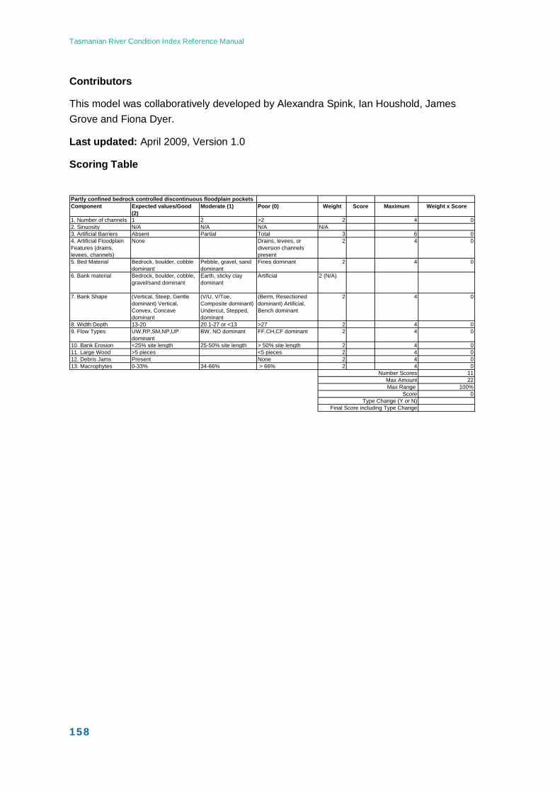
Tasmanian River Condition Index Reference Manual
158
Partly confined bedrock controlled discontinuous floodplain pockets Component Expected values/Good
(2)Moderate (1) Poor (0) Weight Score Maximum Weight x Score
1. Number of channels 1 2 >2 2 4 02. Sinuosity N/A N/A N/A N/A3. Artificial Barriers Absent Partial Total 3 6 04. Artificial Floodplain Features (drains, levees, channels)
None Drains, levees, or diversion channels present
2 4 0
5. Bed Material Bedrock, boulder, cobble dominant
Pebble, gravel, sand dominant
Fines dominant 2 4 0
6. Bank material Bedrock, boulder, cobble, gravel/sand dominant
Earth, sticky clay dominant
Artificial 2 (N/A)
7. Bank Shape (Vertical, Steep, Gentle dominant) Vertical, Convex, Concave dominant
(V/U, V/Toe, Composite dominant) Undercut, Stepped, dominant
(Berm, Resectioned dominant) Artificial, Bench dominant
2 4 0
8. Width:Depth 13-20 20.1-27 or <13 >27 2 4 09. Flow Types UW,RP,SM,NP,UP
dominantBW, NO dominant FF,CH,CF dominant 2 4 0
10. Bank Erosion <25% site length 25-50% site length > 50% site length 2 4 011. Large Wood >5 pieces <5 pieces 2 4 012. Debris Jams Present None 2 4 013. Macrophytes 0-33% 34-66% > 66% 2 4 0
Number Scores 11Max Amount 22Max Range 100%
Score 0Type Change (Y or N)
Final Score including Type Change
Contributors
This model was collaboratively developed by Alexandra Spink, Ian Houshold, James Grove and Fiona Dyer.
Last updated: April 2009, Version 1.0
Scoring Table
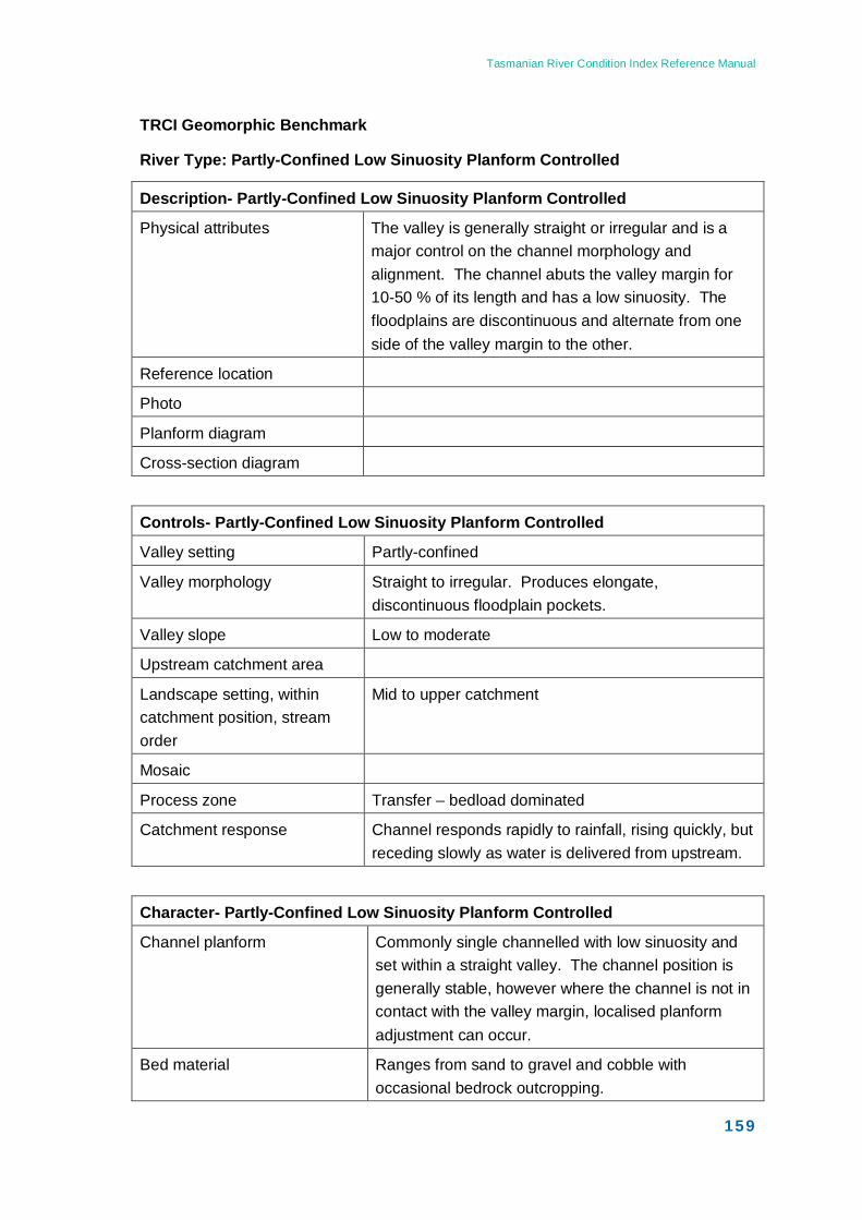
Tasmanian River Condition Index Reference Manual
159
TRCI Geomorphic Benchmark
River Type: Partly-Confined Low Sinuosity Planform Controlled
Description- Partly-Confined Low Sinuosity Planform Controlled
Physical attributes The valley is generally straight or irregular and is a major control on the channel morphology and alignment. The channel abuts the valley margin for 10-50 % of its length and has a low sinuosity. The floodplains are discontinuous and alternate from one side of the valley margin to the other.
Reference location
Photo
Planform diagram
Cross-section diagram
Controls- Partly-Confined Low Sinuosity Planform Controlled
Valley setting Partly-confined
Valley morphology Straight to irregular. Produces elongate, discontinuous floodplain pockets.
Valley slope Low to moderate
Upstream catchment area
Landscape setting, within catchment position, stream order
Mid to upper catchment
Mosaic
Process zone Transfer – bedload dominated
Catchment response Channel responds rapidly to rainfall, rising quickly, but receding slowly as water is delivered from upstream.
Character- Partly-Confined Low Sinuosity Planform Controlled
Channel planform Commonly single channelled with low sinuosity and set within a straight valley. The channel position is generally stable, however where the channel is not in contact with the valley margin, localised planform adjustment can occur.
Bed material Ranges from sand to gravel and cobble with occasional bedrock outcropping.
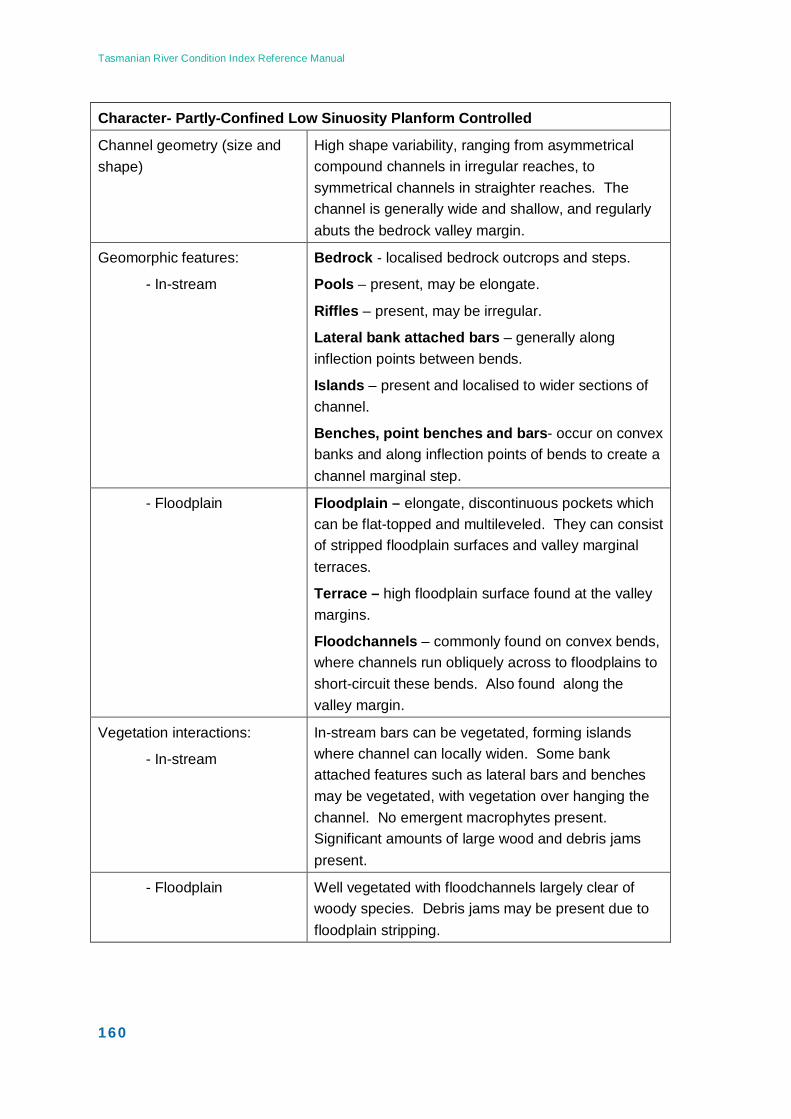
Tasmanian River Condition Index Reference Manual
160
Character- Partly-Confined Low Sinuosity Planform Controlled
Channel geometry (size and shape)
High shape variability, ranging from asymmetrical compound channels in irregular reaches, to symmetrical channels in straighter reaches. The channel is generally wide and shallow, and regularly abuts the bedrock valley margin.
Geomorphic features:
- In-stream
Bedrock - localised bedrock outcrops and steps.
Pools – present, may be elongate.
Riffles – present, may be irregular.
Lateral bank attached bars – generally along inflection points between bends.
Islands – present and localised to wider sections of channel.
Benches, point benches and bars- occur on convex banks and along inflection points of bends to create a channel marginal step.
- Floodplain Floodplain – elongate, discontinuous pockets which can be flat-topped and multileveled. They can consist of stripped floodplain surfaces and valley marginal terraces.
Terrace – high floodplain surface found at the valley margins.
Floodchannels – commonly found on convex bends, where channels run obliquely across to floodplains to short-circuit these bends. Also found along the valley margin.
Vegetation interactions:
- In-stream
In-stream bars can be vegetated, forming islands where channel can locally widen. Some bank attached features such as lateral bars and benches may be vegetated, with vegetation over hanging the channel. No emergent macrophytes present. Significant amounts of large wood and debris jams present.
- Floodplain Well vegetated with floodchannels largely clear of woody species. Debris jams may be present due to floodplain stripping.
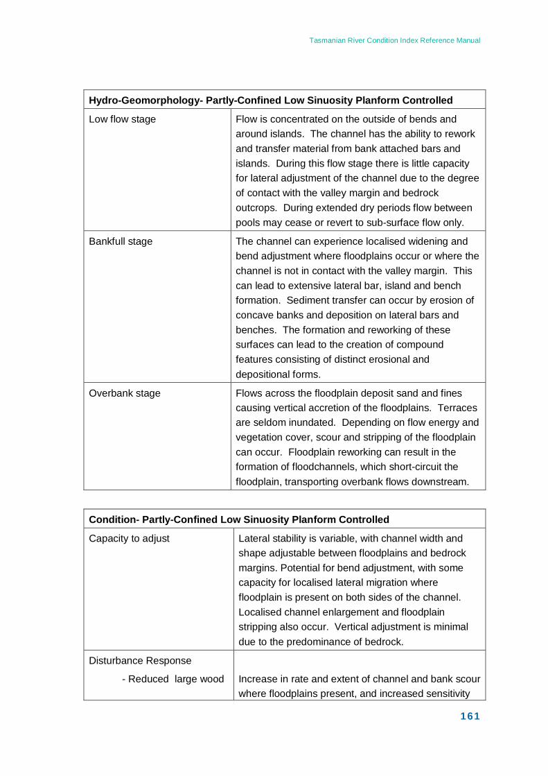
Tasmanian River Condition Index Reference Manual
161
Hydro-Geomorphology- Partly-Confined Low Sinuosity Planform Controlled
Low flow stage Flow is concentrated on the outside of bends and around islands. The channel has the ability to rework and transfer material from bank attached bars and islands. During this flow stage there is little capacity for lateral adjustment of the channel due to the degree of contact with the valley margin and bedrock outcrops. During extended dry periods flow between pools may cease or revert to sub-surface flow only.
Bankfull stage The channel can experience localised widening and bend adjustment where floodplains occur or where the channel is not in contact with the valley margin. This can lead to extensive lateral bar, island and bench formation. Sediment transfer can occur by erosion of concave banks and deposition on lateral bars and benches. The formation and reworking of these surfaces can lead to the creation of compound features consisting of distinct erosional and depositional forms.
Overbank stage Flows across the floodplain deposit sand and fines causing vertical accretion of the floodplains. Terraces are seldom inundated. Depending on flow energy and vegetation cover, scour and stripping of the floodplain can occur. Floodplain reworking can result in the formation of floodchannels, which short-circuit the floodplain, transporting overbank flows downstream.
Condition- Partly-Confined Low Sinuosity Planform Controlled
Capacity to adjust Lateral stability is variable, with channel width and shape adjustable between floodplains and bedrock margins. Potential for bend adjustment, with some capacity for localised lateral migration where floodplain is present on both sides of the channel. Localised channel enlargement and floodplain stripping also occur. Vertical adjustment is minimal due to the predominance of bedrock.
Disturbance Response
- Reduced large wood
Increase in rate and extent of channel and bank scour where floodplains present, and increased sensitivity
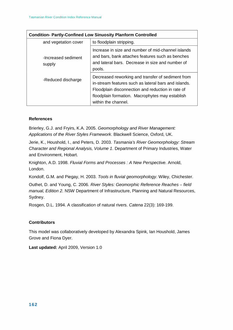
Tasmanian River Condition Index Reference Manual
162
Condition- Partly-Confined Low Sinuosity Planform Controlled and vegetation cover
-Increased sediment supply
-Reduced discharge
to floodplain stripping.
Increase in size and number of mid-channel islands and bars, bank attaches features such as benches and lateral bars. Decrease in size and number of pools.
Decreased reworking and transfer of sediment from in-stream features such as lateral bars and islands. Floodplain disconnection and reduction in rate of floodplain formation. Macrophytes may establish within the channel.
References
Brierley, G.J. and Fryirs, K.A. 2005. Geomorphology and River Management: Applications of the River Styles Framework. Blackwell Science, Oxford, UK.
Jerie, K., Houshold, I., and Peters, D. 2003. Tasmania’s River Geomorphology: Stream Character and Regional Analysis, Volume 1. Department of Primary Industries, Water and Environment, Hobart.
Knighton, A.D. 1998. Fluvial Forms and Processes : A New Perspective. Arnold, London.
Kondolf, G.M. and Piegay, H. 2003. Tools in fluvial geomorphology. Wiley, Chichester.
Outhet, D. and Young, C. 2006. River Styles: Geomorphic Reference Reaches – field manual, Edition 2. NSW Department of Infrastructure, Planning and Natural Resources, Sydney.
Rosgen, D.L. 1994. A classification of natural rivers. Catena 22(3): 169-199.
Contributors
This model was collaboratively developed by Alexandra Spink, Ian Houshold, James Grove and Fiona Dyer.
Last updated: April 2009, Version 1.0
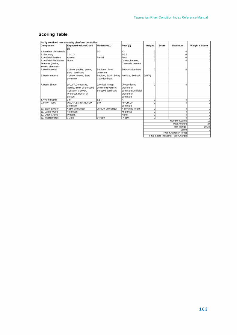
Tasmanian River Condition Index Reference Manual
163
Partly confined low sinuosity planform controlled Component Expected values/Good
(2)Moderate (1) Poor (0) Weight Score Maximum Weight x Score
1. Number of channels 1 2-3 >3 2 4 02. Sinuosity 1.1-1.3 1-1.1 3 6 03. Artificial Barriers Absent Partial Total 3 6 04. Artificial Floodplain Features (drains, levees, channels)
None Drains, Levees, Channels present
2 4 0
5. Bed Material Cobble, pebble, gravel, sand dominant
Boulders, fines dominant
Bedrock dominant 2 4 0
6. Bank material Cobble, Gravel, Sand dominant
Boulder, Earth, Sticky Clay dominant
Artificial, Bedrock 2(N/A)
7. Bank Shape (VU,VT,Composite, Gentle, Berm all present) Concave, Convex, Undercut, Bench all present
(Vertical, Steep, dominant) Vertical, Stepped dominant
(Resectioned present or dominant) Artificial present or dominant
2 4 0
8. Width:Depth 1-5 5.1-7 >7 2 4 09. Flow Types UW,RP,SM,NP,NO,UP
dominantBW FF,CH,CF
dominant2 4 0
10. Bank Erosion <25% site length 25-50% site length > 50% site length 2 4 011. Large Wood >5 pieces <5 pieces 2 4 012. Debris Jams Present None 2 4 013. Macrophytes 1-33% 34-66% > 66% 2 4 0
Number Scores 12Max Amount 24Max Range 100%
Score 0
Final Score including Type ChangeType Change (Y or N)
Scoring Table
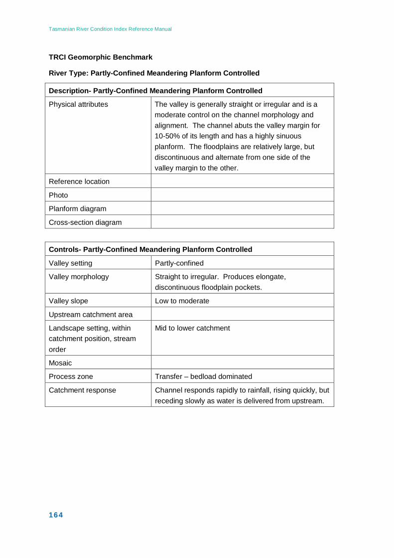
Tasmanian River Condition Index Reference Manual
164
TRCI Geomorphic Benchmark
River Type: Partly-Confined Meandering Planform Controlled
Description- Partly-Confined Meandering Planform Controlled
Physical attributes The valley is generally straight or irregular and is a moderate control on the channel morphology and alignment. The channel abuts the valley margin for 10-50% of its length and has a highly sinuous planform. The floodplains are relatively large, but discontinuous and alternate from one side of the valley margin to the other.
Reference location
Photo
Planform diagram
Cross-section diagram
Controls- Partly-Confined Meandering Planform Controlled
Valley setting Partly-confined
Valley morphology Straight to irregular. Produces elongate, discontinuous floodplain pockets.
Valley slope Low to moderate
Upstream catchment area
Landscape setting, within catchment position, stream order
Mid to lower catchment
Mosaic
Process zone Transfer – bedload dominated
Catchment response Channel responds rapidly to rainfall, rising quickly, but receding slowly as water is delivered from upstream.
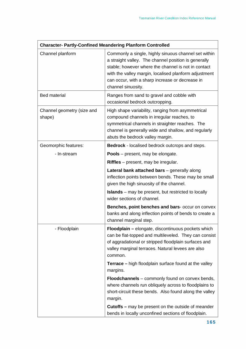
Tasmanian River Condition Index Reference Manual
165
Character- Partly-Confined Meandering Planform Controlled
Channel planform Commonly a single, highly sinuous channel set within a straight valley. The channel position is generally stable; however where the channel is not in contact with the valley margin, localised planform adjustment can occur, with a sharp increase or decrease in channel sinuosity.
Bed material Ranges from sand to gravel and cobble with occasional bedrock outcropping.
Channel geometry (size and shape)
High shape variability, ranging from asymmetrical compound channels in irregular reaches, to symmetrical channels in straighter reaches. The channel is generally wide and shallow, and regularly abuts the bedrock valley margin.
Geomorphic features:
- In-stream
Bedrock - localised bedrock outcrops and steps.
Pools – present, may be elongate.
Riffles – present, may be irregular.
Lateral bank attached bars – generally along inflection points between bends. These may be small given the high sinuosity of the channel.
Islands – may be present, but restricted to locally wider sections of channel.
Benches, point benches and bars- occur on convex banks and along inflection points of bends to create a channel marginal step.
- Floodplain Floodplain – elongate, discontinuous pockets which can be flat-topped and multileveled. They can consist of aggradational or stripped floodplain surfaces and valley marginal terraces. Natural levees are also common.
Terrace – high floodplain surface found at the valley margins.
Floodchannels – commonly found on convex bends, where channels run obliquely across to floodplains to short-circuit these bends. Also found along the valley margin.
Cutoffs – may be present on the outside of meander bends in locally unconfined sections of floodplain.
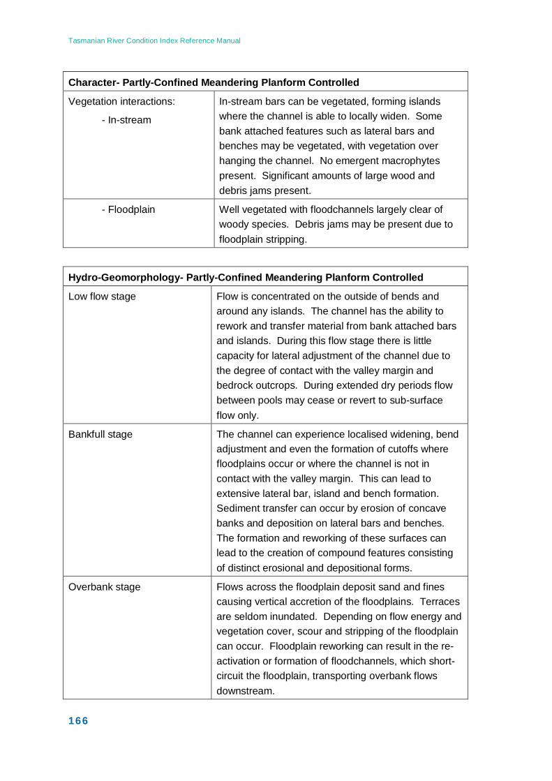
Tasmanian River Condition Index Reference Manual
166
Character- Partly-Confined Meandering Planform Controlled
Vegetation interactions:
- In-stream
In-stream bars can be vegetated, forming islands where the channel is able to locally widen. Some bank attached features such as lateral bars and benches may be vegetated, with vegetation over hanging the channel. No emergent macrophytes present. Significant amounts of large wood and debris jams present.
- Floodplain Well vegetated with floodchannels largely clear of woody species. Debris jams may be present due to floodplain stripping.
Hydro-Geomorphology- Partly-Confined Meandering Planform Controlled
Low flow stage Flow is concentrated on the outside of bends and around any islands. The channel has the ability to rework and transfer material from bank attached bars and islands. During this flow stage there is little capacity for lateral adjustment of the channel due to the degree of contact with the valley margin and bedrock outcrops. During extended dry periods flow between pools may cease or revert to sub-surface flow only.
Bankfull stage The channel can experience localised widening, bend adjustment and even the formation of cutoffs where floodplains occur or where the channel is not in contact with the valley margin. This can lead to extensive lateral bar, island and bench formation. Sediment transfer can occur by erosion of concave banks and deposition on lateral bars and benches. The formation and reworking of these surfaces can lead to the creation of compound features consisting of distinct erosional and depositional forms.
Overbank stage Flows across the floodplain deposit sand and fines causing vertical accretion of the floodplains. Terraces are seldom inundated. Depending on flow energy and vegetation cover, scour and stripping of the floodplain can occur. Floodplain reworking can result in the re-activation or formation of floodchannels, which short-circuit the floodplain, transporting overbank flows downstream.
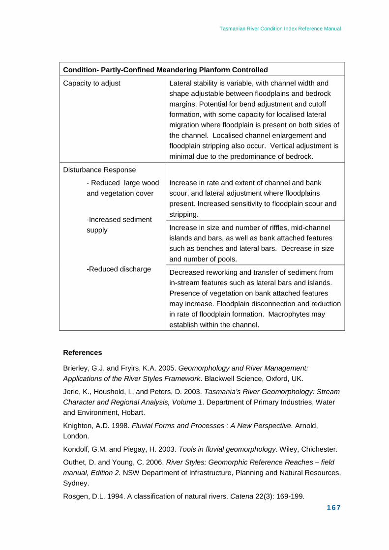
Tasmanian River Condition Index Reference Manual
167
Condition- Partly-Confined Meandering Planform Controlled
Capacity to adjust Lateral stability is variable, with channel width and shape adjustable between floodplains and bedrock margins. Potential for bend adjustment and cutoff formation, with some capacity for localised lateral migration where floodplain is present on both sides of the channel. Localised channel enlargement and floodplain stripping also occur. Vertical adjustment is minimal due to the predominance of bedrock.
Disturbance Response
- Reduced large wood and vegetation cover
-Increased sediment supply
-Reduced discharge
Increase in rate and extent of channel and bank scour, and lateral adjustment where floodplains present. Increased sensitivity to floodplain scour and stripping.
Increase in size and number of riffles, mid-channel islands and bars, as well as bank attached features such as benches and lateral bars. Decrease in size and number of pools.
Decreased reworking and transfer of sediment from in-stream features such as lateral bars and islands. Presence of vegetation on bank attached features may increase. Floodplain disconnection and reduction in rate of floodplain formation. Macrophytes may establish within the channel.
References
Brierley, G.J. and Fryirs, K.A. 2005. Geomorphology and River Management: Applications of the River Styles Framework. Blackwell Science, Oxford, UK.
Jerie, K., Houshold, I., and Peters, D. 2003. Tasmania’s River Geomorphology: Stream Character and Regional Analysis, Volume 1. Department of Primary Industries, Water and Environment, Hobart.
Knighton, A.D. 1998. Fluvial Forms and Processes : A New Perspective. Arnold, London.
Kondolf, G.M. and Piegay, H. 2003. Tools in fluvial geomorphology. Wiley, Chichester.
Outhet, D. and Young, C. 2006. River Styles: Geomorphic Reference Reaches – field manual, Edition 2. NSW Department of Infrastructure, Planning and Natural Resources, Sydney.
Rosgen, D.L. 1994. A classification of natural rivers. Catena 22(3): 169-199.
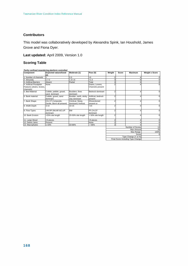
Tasmanian River Condition Index Reference Manual
168
Partly confined meandering planform controlled Component Expected values/Good
(2)Moderate (1) Poor (0) Weight Score Maximum Weight x Score
1. Number of channels 1 2-3 >3 2 4 02. Sinuosity 1.7-2 1.3-1.6 <1.3 3 6 03. Artificial Barriers Absent Partial Total 3 6 04. Artificial Floodplain Features (drains, levees, channels)
None Drains, Levees, Channels present
2 4 0
5. Bed Material Cobble, pebble, gravel, sand dominant
Boulders, fines dominant
Bedrock dominant 2 4 0
6. Bank material Cobble, gravel, sand dominant
Boulder, earth, sticky clay dominant
Artificial, bedrock present
2 4 0
7. Bank Shape (VU,VT,Composite, Gentle, Berm all present)
(Vertical, Steep, dominant) Vertical,
(Resectioned present or
2 4 0
8. Width:Depth 3-10 10-15 >15 2 4 0
9. Flow Types UW,RP,SM,NP,NO,UP dominant
BW FF,CH,CF dominant
2 4 0
10. Bank Erosion <25% site length 25-50% site length > 50% site length 2 4 0
11. Large Wood >5 pieces <5 pieces 2 4 012. Debris Jams Present None 2 4 013. Macrophytes 1-33% 33-66% > 66% 2 4 0
Number of Scores 13Max Amount 26Max Range 100%
Score 0Type Change (Y or N)
Final Score including Type Change
Contributors
This model was collaboratively developed by Alexandra Spink, Ian Houshold, James Grove and Fiona Dyer.
Last updated: April 2009, Version 1.0
Scoring Table
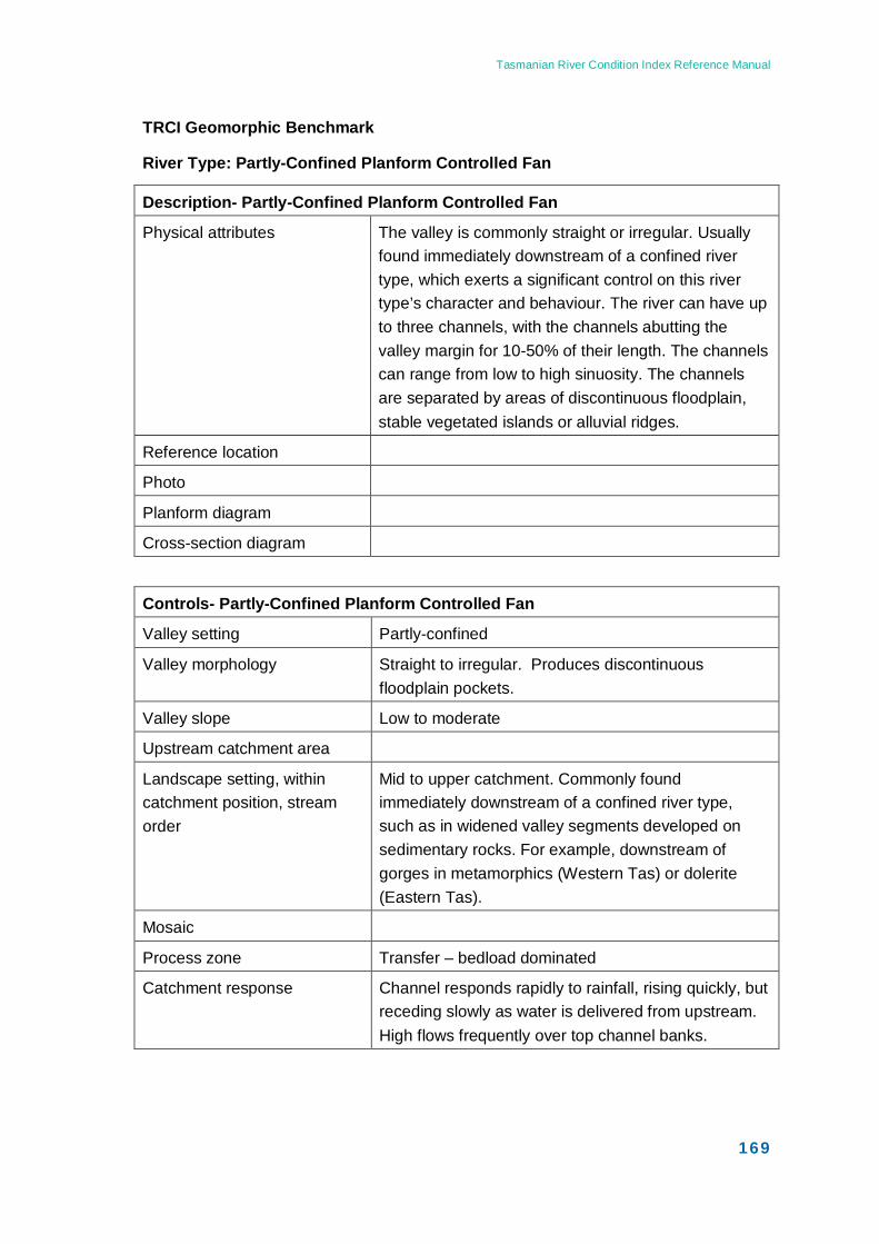
Tasmanian River Condition Index Reference Manual
169
TRCI Geomorphic Benchmark
River Type: Partly-Confined Planform Controlled Fan
Description- Partly-Confined Planform Controlled Fan
Physical attributes The valley is commonly straight or irregular. Usually found immediately downstream of a confined river type, which exerts a significant control on this river type’s character and behaviour. The river can have up to three channels, with the channels abutting the valley margin for 10-50% of their length. The channels can range from low to high sinuosity. The channels are separated by areas of discontinuous floodplain, stable vegetated islands or alluvial ridges.
Reference location
Photo
Planform diagram
Cross-section diagram
Controls- Partly-Confined Planform Controlled Fan
Valley setting Partly-confined
Valley morphology Straight to irregular. Produces discontinuous floodplain pockets.
Valley slope Low to moderate
Upstream catchment area
Landscape setting, within catchment position, stream order
Mid to upper catchment. Commonly found immediately downstream of a confined river type, such as in widened valley segments developed on sedimentary rocks. For example, downstream of gorges in metamorphics (Western Tas) or dolerite (Eastern Tas).
Mosaic
Process zone Transfer – bedload dominated
Catchment response Channel responds rapidly to rainfall, rising quickly, but receding slowly as water is delivered from upstream. High flows frequently over top channel banks.
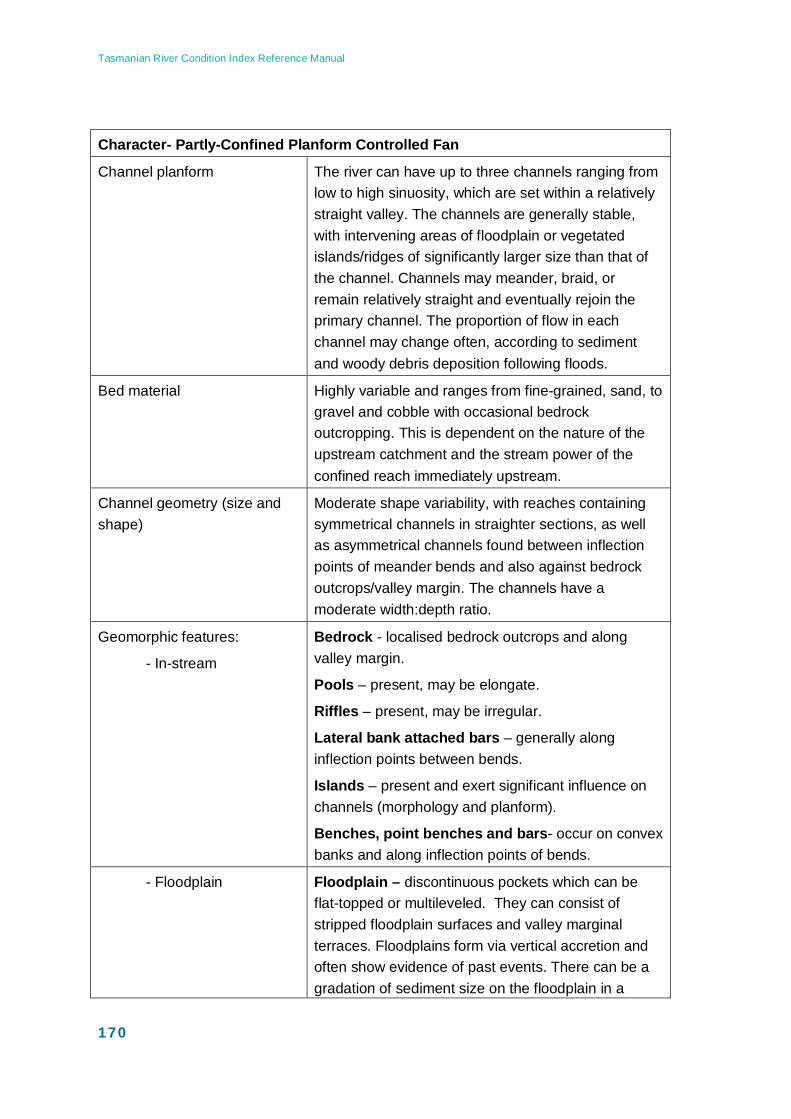
Tasmanian River Condition Index Reference Manual
170
Character- Partly-Confined Planform Controlled Fan
Channel planform The river can have up to three channels ranging from low to high sinuosity, which are set within a relatively straight valley. The channels are generally stable, with intervening areas of floodplain or vegetated islands/ridges of significantly larger size than that of the channel. Channels may meander, braid, or remain relatively straight and eventually rejoin the primary channel. The proportion of flow in each channel may change often, according to sediment and woody debris deposition following floods.
Bed material Highly variable and ranges from fine-grained, sand, to gravel and cobble with occasional bedrock outcropping. This is dependent on the nature of the upstream catchment and the stream power of the confined reach immediately upstream.
Channel geometry (size and shape)
Moderate shape variability, with reaches containing symmetrical channels in straighter sections, as well as asymmetrical channels found between inflection points of meander bends and also against bedrock outcrops/valley margin. The channels have a moderate width:depth ratio.
Geomorphic features:
- In-stream
Bedrock - localised bedrock outcrops and along valley margin.
Pools – present, may be elongate.
Riffles – present, may be irregular.
Lateral bank attached bars – generally along inflection points between bends.
Islands – present and exert significant influence on channels (morphology and planform).
Benches, point benches and bars- occur on convex banks and along inflection points of bends.
- Floodplain Floodplain – discontinuous pockets which can be flat-topped or multileveled. They can consist of stripped floodplain surfaces and valley marginal terraces. Floodplains form via vertical accretion and often show evidence of past events. There can be a gradation of sediment size on the floodplain in a
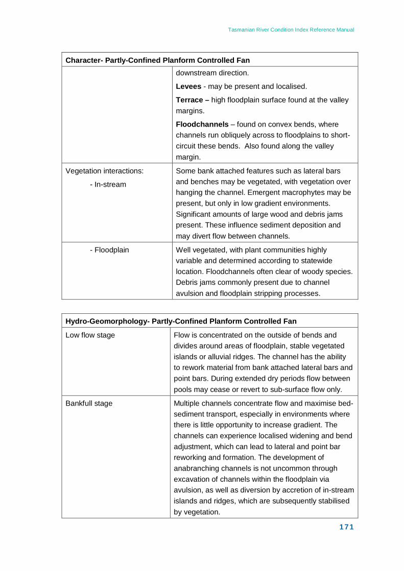
Tasmanian River Condition Index Reference Manual
171
Character- Partly-Confined Planform Controlled Fan downstream direction.
Levees - may be present and localised.
Terrace – high floodplain surface found at the valley margins.
Floodchannels – found on convex bends, where channels run obliquely across to floodplains to short-circuit these bends. Also found along the valley margin.
Vegetation interactions:
- In-stream
Some bank attached features such as lateral bars and benches may be vegetated, with vegetation over hanging the channel. Emergent macrophytes may be present, but only in low gradient environments. Significant amounts of large wood and debris jams present. These influence sediment deposition and may divert flow between channels.
- Floodplain Well vegetated, with plant communities highly variable and determined according to statewide location. Floodchannels often clear of woody species. Debris jams commonly present due to channel avulsion and floodplain stripping processes.
Hydro-Geomorphology- Partly-Confined Planform Controlled Fan
Low flow stage Flow is concentrated on the outside of bends and divides around areas of floodplain, stable vegetated islands or alluvial ridges. The channel has the ability to rework material from bank attached lateral bars and point bars. During extended dry periods flow between pools may cease or revert to sub-surface flow only.
Bankfull stage Multiple channels concentrate flow and maximise bed-sediment transport, especially in environments where there is little opportunity to increase gradient. The channels can experience localised widening and bend adjustment, which can lead to lateral and point bar reworking and formation. The development of anabranching channels is not uncommon through excavation of channels within the floodplain via avulsion, as well as diversion by accretion of in-stream islands and ridges, which are subsequently stabilised by vegetation.
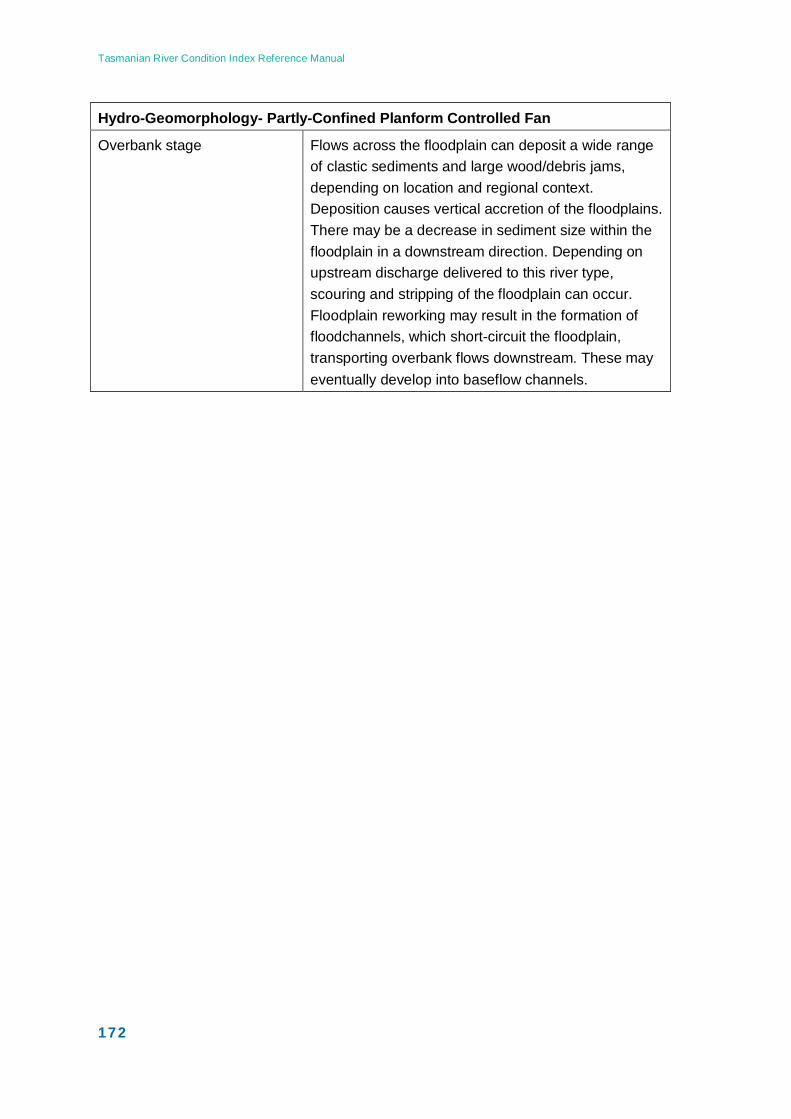
Tasmanian River Condition Index Reference Manual
172
Hydro-Geomorphology- Partly-Confined Planform Controlled Fan
Overbank stage Flows across the floodplain can deposit a wide range of clastic sediments and large wood/debris jams, depending on location and regional context. Deposition causes vertical accretion of the floodplains. There may be a decrease in sediment size within the floodplain in a downstream direction. Depending on upstream discharge delivered to this river type, scouring and stripping of the floodplain can occur. Floodplain reworking may result in the formation of floodchannels, which short-circuit the floodplain, transporting overbank flows downstream. These may eventually develop into baseflow channels.
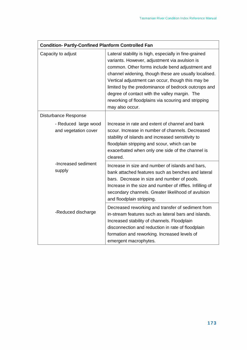
Tasmanian River Condition Index Reference Manual
173
Condition- Partly-Confined Planform Controlled Fan
Capacity to adjust Lateral stability is high, especially in fine-grained variants. However, adjustment via avulsion is common. Other forms include bend adjustment and channel widening, though these are usually localised. Vertical adjustment can occur, though this may be limited by the predominance of bedrock outcrops and degree of contact with the valley margin. The reworking of floodplains via scouring and stripping may also occur.
Disturbance Response
- Reduced large wood and vegetation cover
-Increased sediment supply
-Reduced discharge
Increase in rate and extent of channel and bank scour. Increase in number of channels. Decreased stability of islands and increased sensitivity to floodplain stripping and scour, which can be exacerbated when only one side of the channel is cleared.
Increase in size and number of islands and bars, bank attached features such as benches and lateral bars. Decrease in size and number of pools. Increase in the size and number of riffles. Infilling of secondary channels. Greater likelihood of avulsion and floodplain stripping.
Decreased reworking and transfer of sediment from in-stream features such as lateral bars and islands. Increased stability of channels. Floodplain disconnection and reduction in rate of floodplain formation and reworking. Increased levels of emergent macrophytes.
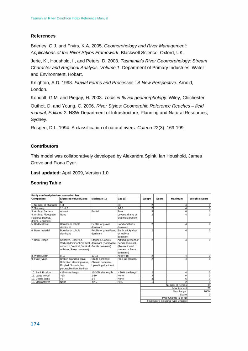
Tasmanian River Condition Index Reference Manual
174
Partly confined planform controlled fanComponent Expected values/Good
(2)Moderate (1) Bad (0) Weight Score Maximum Weight x Score
1. Number of channels 1-3 >3 2 4 02. Sinuosity 1.1-1.3 1-1.1 2 4 03. Artificial Barriers Absent Partial Total 3 6 04. Artificial Floodplain Features (levees, drains, Channels)
None Levees, drains or channels present
2 4 0
5. Bed Material Boulder or cobble dominant
Pebble or gravel dominant
Sand and fines dominant
2 4 0
6. Bank material Boulder or cobble dominant
Pebble or gravel/sand dominant
Earth, sticky clay, or artificial dominant
2 4 0
7. Bank Shape Concave, Undercut, Vertical dominant (Vertical undercut, Vertical, Vertical with toe, Steep dominant)
Stepped, Convex dominant (Composite, Gentle dominant)
Artificial present or Bench dominant (Re-sectioned present or Berm dominant)
2 4 0
8. Width:Depth 8-12 13-18 >8 or >18 2 4 09. Flow Types Broken Standing wave,
Unbroken standing wave, Rippled, Smooth, No perceptible flow, No flow
Chute dominant, Chaotic dominant, Upwelling dominant
Free-fall present, 2 4 0
10. Bank Erosion <15% site length 15-30% site length > 30% site length 2 4 011. Large Wood >10 1-10 None 3 6 012. Debris Jams >5 1-5 None 3 6 013. Macrophytes None <5% >5% 1 2 0
Number of Scores 13Max Amount 26Max Range 100%
Score 0Type Change (Y or N)
Final Score including Type Change
References
Brierley, G.J. and Fryirs, K.A. 2005. Geomorphology and River Management: Applications of the River Styles Framework. Blackwell Science, Oxford, UK.
Jerie, K., Houshold, I., and Peters, D. 2003. Tasmania’s River Geomorphology: Stream Character and Regional Analysis, Volume 1. Department of Primary Industries, Water and Environment, Hobart.
Knighton, A.D. 1998. Fluvial Forms and Processes : A New Perspective. Arnold, London.
Kondolf, G.M. and Piegay, H. 2003. Tools in fluvial geomorphology. Wiley, Chichester.
Outhet, D. and Young, C. 2006. River Styles: Geomorphic Reference Reaches – field manual, Edition 2. NSW Department of Infrastructure, Planning and Natural Resources, Sydney.
Rosgen, D.L. 1994. A classification of natural rivers. Catena 22(3): 169-199.
Contributors
This model was collaboratively developed by Alexandra Spink, Ian Houshold, James Grove and Fiona Dyer.
Last updated: April 2009, Version 1.0
Scoring Table
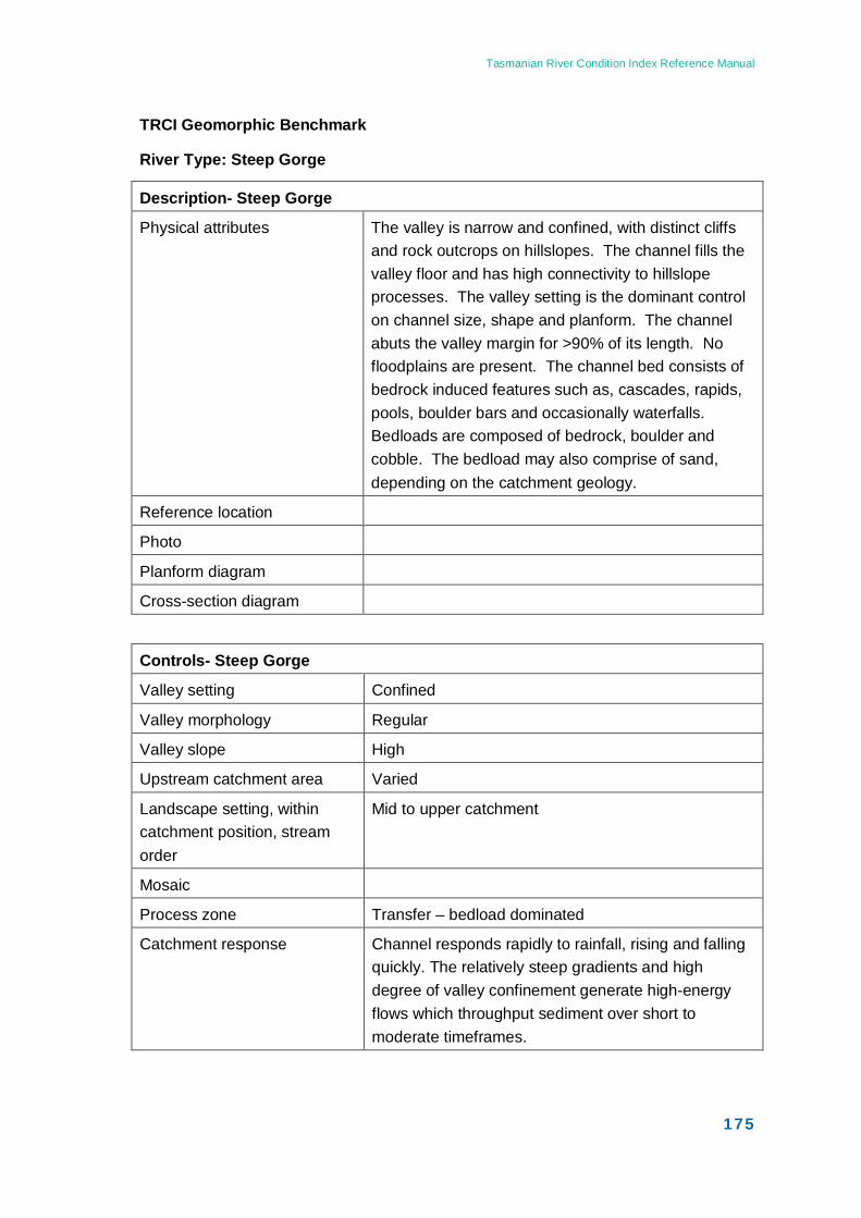
Tasmanian River Condition Index Reference Manual
175
TRCI Geomorphic Benchmark
River Type: Steep Gorge
Description- Steep Gorge
Physical attributes The valley is narrow and confined, with distinct cliffs and rock outcrops on hillslopes. The channel fills the valley floor and has high connectivity to hillslope processes. The valley setting is the dominant control on channel size, shape and planform. The channel abuts the valley margin for >90% of its length. No floodplains are present. The channel bed consists of bedrock induced features such as, cascades, rapids, pools, boulder bars and occasionally waterfalls. Bedloads are composed of bedrock, boulder and cobble. The bedload may also comprise of sand, depending on the catchment geology.
Reference location
Photo
Planform diagram
Cross-section diagram
Controls- Steep Gorge
Valley setting Confined
Valley morphology Regular
Valley slope High
Upstream catchment area Varied
Landscape setting, within catchment position, stream order
Mid to upper catchment
Mosaic
Process zone Transfer – bedload dominated
Catchment response Channel responds rapidly to rainfall, rising and falling quickly. The relatively steep gradients and high degree of valley confinement generate high-energy flows which throughput sediment over short to moderate timeframes.
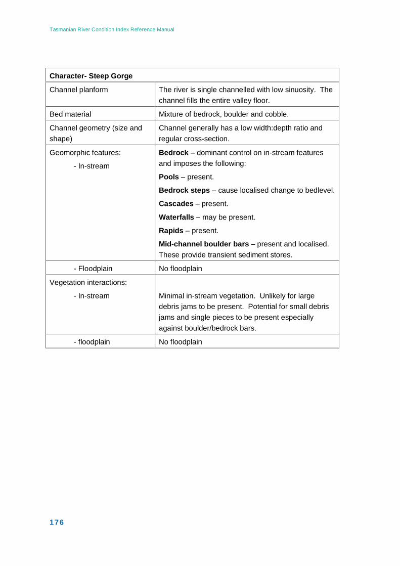
Tasmanian River Condition Index Reference Manual
176
Character- Steep Gorge
Channel planform The river is single channelled with low sinuosity. The channel fills the entire valley floor.
Bed material Mixture of bedrock, boulder and cobble.
Channel geometry (size and shape)
Channel generally has a low width:depth ratio and regular cross-section.
Geomorphic features:
- In-stream
Bedrock – dominant control on in-stream features and imposes the following:
Pools – present.
Bedrock steps – cause localised change to bedlevel.
Cascades – present.
Waterfalls – may be present.
Rapids – present.
Mid-channel boulder bars – present and localised. These provide transient sediment stores.
- Floodplain No floodplain
Vegetation interactions:
- In-stream
Minimal in-stream vegetation. Unlikely for large debris jams to be present. Potential for small debris jams and single pieces to be present especially against boulder/bedrock bars.
- floodplain No floodplain
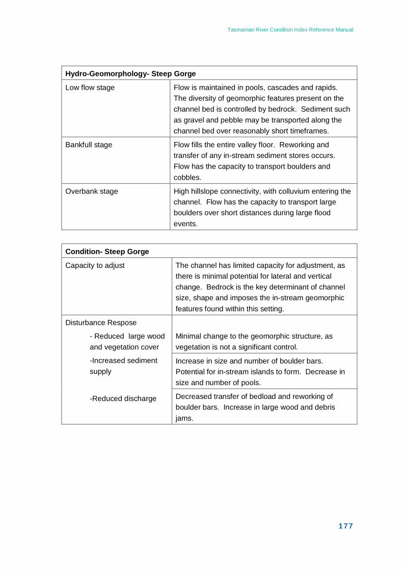
Tasmanian River Condition Index Reference Manual
177
Hydro-Geomorphology- Steep Gorge
Low flow stage Flow is maintained in pools, cascades and rapids. The diversity of geomorphic features present on the channel bed is controlled by bedrock. Sediment such as gravel and pebble may be transported along the channel bed over reasonably short timeframes.
Bankfull stage Flow fills the entire valley floor. Reworking and transfer of any in-stream sediment stores occurs. Flow has the capacity to transport boulders and cobbles.
Overbank stage High hillslope connectivity, with colluvium entering the channel. Flow has the capacity to transport large boulders over short distances during large flood events.
Condition- Steep Gorge
Capacity to adjust The channel has limited capacity for adjustment, as there is minimal potential for lateral and vertical change. Bedrock is the key determinant of channel size, shape and imposes the in-stream geomorphic features found within this setting.
Disturbance Respose
- Reduced large wood and vegetation cover
-Increased sediment supply
-Reduced discharge
Minimal change to the geomorphic structure, as vegetation is not a significant control.
Increase in size and number of boulder bars. Potential for in-stream islands to form. Decrease in size and number of pools.
Decreased transfer of bedload and reworking of boulder bars. Increase in large wood and debris jams.
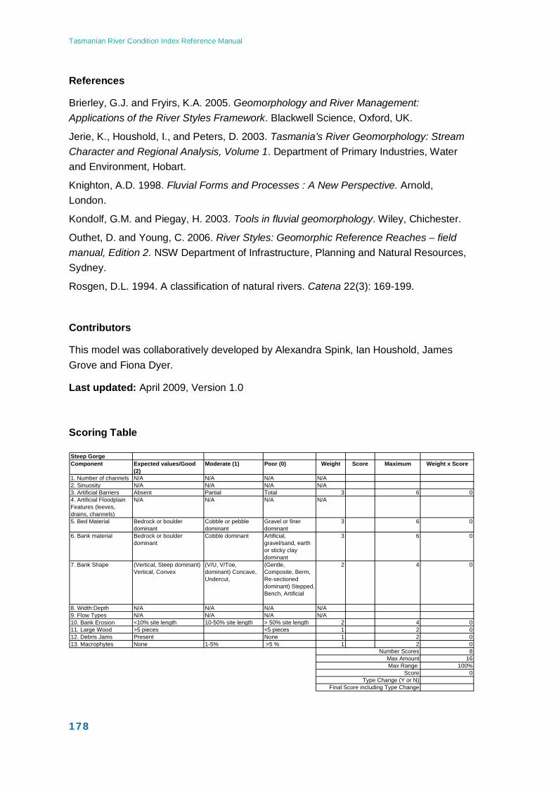
Tasmanian River Condition Index Reference Manual
178
Steep GorgeComponent Expected values/Good
(2)Moderate (1) Poor (0) Weight Score Maximum Weight x Score
1. Number of channels N/A N/A N/A N/A2. Sinuosity N/A N/A N/A N/A3. Artificial Barriers Absent Partial Total 3 6 04. Artificial Floodplain Features (leeves, drains, channels)
N/A N/A N/A N/A
5. Bed Material Bedrock or boulder dominant
Cobble or pebble dominant
Gravel or finer dominant
3 6 0
6. Bank material Bedrock or boulder dominant
Cobble dominant Artificial, gravel/sand, earth or sticky clay dominant
3 6 0
7. Bank Shape (Vertical, Steep dominant) Vertical, Convex
(V/U, V/Toe, dominant) Concave, Undercut,
(Gentle, Composite, Berm, Re-sectioned dominant) Stepped, Bench, Artificial
2 4 0
8. Width:Depth N/A N/A N/A N/A9. Flow Types N/A N/A N/A N/A10. Bank Erosion <10% site length 10-50% site length > 50% site length 2 4 011. Large Wood >5 pieces <5 pieces 1 2 012. Debris Jams Present None 1 2 013. Macrophytes None 1-5% >5 % 1 2 0
Number Scores 8Max Amount 16Max Range 100%
Score 0Type Change (Y or N)
Final Score including Type Change
References
Brierley, G.J. and Fryirs, K.A. 2005. Geomorphology and River Management: Applications of the River Styles Framework. Blackwell Science, Oxford, UK.
Jerie, K., Houshold, I., and Peters, D. 2003. Tasmania’s River Geomorphology: Stream Character and Regional Analysis, Volume 1. Department of Primary Industries, Water and Environment, Hobart.
Knighton, A.D. 1998. Fluvial Forms and Processes : A New Perspective. Arnold, London.
Kondolf, G.M. and Piegay, H. 2003. Tools in fluvial geomorphology. Wiley, Chichester.
Outhet, D. and Young, C. 2006. River Styles: Geomorphic Reference Reaches – field manual, Edition 2. NSW Department of Infrastructure, Planning and Natural Resources, Sydney.
Rosgen, D.L. 1994. A classification of natural rivers. Catena 22(3): 169-199.
Contributors
This model was collaboratively developed by Alexandra Spink, Ian Houshold, James Grove and Fiona Dyer.
Last updated: April 2009, Version 1.0
Scoring Table
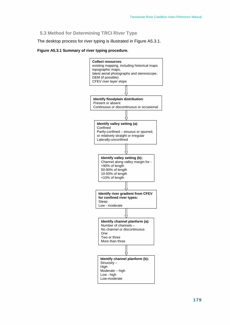
Tasmanian River Condition Index Reference Manual
179
Identify floodplain distribution: Present or absent Continuous or discontinuous or occasional
Identify valley setting (b): Channel along valley margin for - >90% of length 50-90% of length 10-50% of length <10% of length
Identify river gradient from CFEV for confined river types: Steep Low - moderate
Identify valley setting (a): Confined Partly-confined – sinuous or spurred, or relatively straight or irregular Laterally-unconfined
Collect resources: existing mapping, including historical maps topographic maps, latest aerial photographs and stereoscope, DEM (if possible) CFEV river layer slope
Identify channel planform (a): Number of channels – No channel or discontinuous One Two or three More than three
Identify channel planform (b): Sinuosity – High Moderate – high Low - high Low-moderate
5.3 Method for Determining TRCI River Type The desktop process for river typing is illustrated in Figure A5.3.1.
Figure A5.3.1 Summary of river typing procedure.
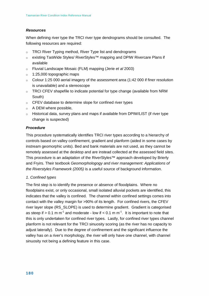
Tasmanian River Condition Index Reference Manual
180
Resources
When defining river type the TRCI river type dendrograms should be consulted. The following resources are required:
o TRCI River Typing method, River Type list and dendrograms o existing TasWide Styles/ RiverStyles™ mapping and DPIW Rivercare Plans if
available o Fluvial Landscape Mosaic (FLM) mapping (Jerie et al 2003) o 1:25,000 topographic maps o Colour 1:25 000 aerial imagery of the assessment area (1:42 000 if finer resolution
is unavailable) and a stereoscope o TRCI CFEV shapefile to indicate potential for type change (available from NRM
South) o CFEV database to determine slope for confined river types o A DEM where possible, o Historical data, survey plans and maps if available from DPIW/LIST (if river type
change is suspected)
Procedure
This procedure systematically identifies TRCI river types according to a hierarchy of controls based on valley confinement, gradient and planform (aided in some cases by instream geomorphic units). Bed and bank materials are not used, as they cannot be remotely assessed at the desktop and are instead collected at the assessed field sites. This procedure is an adaptation of the RiverStyles™ approach developed by Brierly and Fryirs. Their textbook Geomorphologogy and river management: Applications of the Riverstyles Framework (2005) is a useful source of background information.
1. Confined types
The first step is to identify the presence or absence of floodplains. Where no floodplains exist, or only occasional, small isolated alluvial pockets are identified, this indicates that the valley is confined. The channel within confined settings comes into contact with the valley margin for >90% of its length. For confined rivers, the CFEV river layer slope (RS_SLOPE) is used to determine gradient. Gradient is categorised as steep if > 0.1 m m-1 and moderate - low if < 0.1 m m-1. It is important to note that this is only undertaken for confined river types. Lastly, for confined river types channel planform is not relevant for the TRCI sinuosity scoring (as the river has no capacity to adjust laterally). Due to the degree of confinement and the significant influence the valley has on a river’s morphology, the river will only have one channel, with channel sinuosity not being a defining feature in this case.
Tasmanian River Condition Index Reference Manual
181
TRCI river types with a steep slope and no floodplains present are:
o Confined steep o Steep gorge o Talus confined steep o Moraine confined steep
Determining whether a river is a gorge or just confined can be difficult. However, the presence of cliffs and rocky out crops on the hillslopes indicates that the river type is a gorge.
A river type which is steep with occasional floodplain pockets is referred to as:
o Confined steep with occasional floodplain pockets
River types with a low-moderate gradient and no floodplains present include:
o Confined low gradient o Low gradient gorge o Talus confined low gradient o Moraine confined low gradient
River types that have a low-moderate gradient with occasional floodplain pockets include:
o Confined low gradient with occasional floodplain pockets
2. Partly-confined types
If floodplains are present, but occur on alternate sides of the channel as individual, discontinuous pockets separated by the channel which periodically abuts the valley margin, then this river type is partly-confined. However, the shape of the valley and the degree of contact the channel has with the valley margin further determines the river type.
Partly-confined types are either controlled, or planform controlled. If the valley is sinuous with extended bedrock spurs and the channel abuts the valley margin for 50-90% of its length, then the channel is valley controlled by such features as bedrock or terraces. These river types are:
o Partly-confined beach ridge controlled with discontinuous floodplain pockets o Partly-confined bedrock controlled with discontinuous floodplain pockets o Partly- confined terrace controlled with discontinuous floodplain pockets
On the other hand, if the valley is relatively straight or irregular, the channel can abut the valley margin for 10-90% of its length. These are planform controlled river types. When identifying channel planform features, partly-confined river types can have up to three channels and sinuosity can be either high or low-moderate. The sinuosity
Tasmanian River Condition Index Reference Manual
182
determines whether the channel is meandering or low sinuosity/wandering respectively. For high sinuosities >1.3 the river is classed as meandering. These river types are:
o Partly-confined meandering planform controlled
For low-moderate sinuosities <1.3 the river is labelled as low sinuosity or wandering.
o Partly-confined low sinuosity planform controlled o Partly-confined planform controlled fan o Partly-confined broadwater pool o Partly-confined wandering planform controlled
3. Laterally-unconfined types.
Where floodplains are present and continuous along both sides of the channel and valley, then the valley setting is laterally unconfined. Within this setting the channel comes into contact with the valley margin for <10% of its length. For laterally-unconfined river types, channel planform features can vary significantly. A wide range of sinuosities and number of channels may be present. For high sinuosity these are:
o Laterally-unconfined meandering o Laterally-unconfined meandering swamp channel o Laterally-unconfined fan o Laterally-unconfined bank confined
Rivers with low-moderate sinuosity include:
o Laterally-unconfined low sinuosity o Laterally-unconfined low sinuosity swamp channel
Rivers with two or three channels can range from low to high sinuosity and are:
o Laterally-unconfined wandering
Rivers with more than three channels can range from low to high sinuosity and include:
o Laterally-unconfined swamp belt
Rivers which have either no defined channel or a discontinuous channel, such as a series of ponds, include:
o Laterally-unconfined intact valley fill
Sinuosity is not relevant in this case given that there is no continuous channel.
Instream Geomorphic Units
Desktop identification of instream geomorphic units can also assist in assessing whether a new type has been found, or whether the river is a degraded example of a currently listed type. For example, continuous instream bars in a confined type suggests the presence of an artificial sediment slug, rather than a new river type.
Tasmanian River Condition Index Reference Manual
183
Instream geomorphic features consist of, but are not limited to:
o Point bars are bank attached bars that develop along the convex banks of meander bends. These bars are usually unvegetated.
o Lateral bars are bank attached bars which develop along low sinuosity rivers. They occur on alternating sides of the channel and are generally unvegetated.
o Instream bars come in a variety of forms and tend to scale to the dimensions of the channel. Although large woody debris may accumulate on a bar, they are largely unvegetated.
o Islands are vegetated mid-channel bars and can scale to one or more channel widths in length.
Floodplain features
Floodplain features can be used to determine whether a river segment has changed type from pre-European, e.g. where a straight channel flows through a floodplain which was originally characterised by sinuous channels. Relevant floodplain geomorphic features include:
o Prior channels or paleochannels are old, inactive channels which may be partially or entirely filled. They will have more than one meander wavelength (differentiating them from meander cutoffs).
o Floodchannels are slightly curved secondary channels, with flow alignment down valley. They are commonly found at the valley margin.
o Terraces are generally flat features found at the valley margin and perched above the contemporary channel and/or floodplain. These old floodplains are no longer active and can often appear as a flight of terraces. They can be paired or unpaired.
o Backswamps are relatively low lying areas on the distal floodplain, often at the valley margin. Wetlands and swamps can form where lower order tributaries drain into the area.
o Cutoffs are bends which have been dissected, effectively short-circuiting the channel, and leaving the original, larger bend abandoned.
Determining a river type boundary
Boundaries between river types are defined by a change in the diagnostic features (those features used to determine river type, Figure A5.3.1), meaning that a change in the geomorphic structure is identified. It is important to note when determining a river type boundary that it is the downstream changes in the diagnostic features which indicates a river type change.
The boundaries between river types can be distinct or gradual. Distinct boundaries may occur at tributary-trunk confluences, discrete changes in slope, such as bedrock steps, a change in valley width, or morphology related to regional lithological or structural controls. Gradual boundaries occur where gradual downstream changes in valley width, morphology, slope or where features which change the availability of
Tasmanian River Condition Index Reference Manual
184
sediment occur. These transition zones may occur over several kilometres, and as a continuum of river type often exists, the boundary should be placed in the middle of the transition zone between reaches. Lastly, given that rivers can experience a continuum of river type, TRCI sites selected for assessment should not be located near a river type boundary and be at least 200 metres from a boundary.
Regional variation
For some river types, regional landscape character will determine the correct ranges of expected, moderate and poor condition for components within scoring tables. For example, the expected bed material for river types located in granite catchments will differ from that in dolerite catchments. For this reason the relevant Fluvial Landscape Mosaic is determined from a GIS shapefile, and where necessary, used to assign the correct suite of expected, moderate and poor ranges within scoring tables. Contact the relevant DPIW branch for a checklist of relevant FLM’s and guidance.
Geomorphological Training
Even though the procedure for the identification of river types may appear straight forward on the surface, it is strongly recommended that a trained geomorphologist with a fluvial background undertake such tasks. Given that the TRCI river types are based to some extent on River Styles™, it is also strongly recommended that the geomorphologist have a River Styles™ accreditation. There is a real danger that someone who is inexperienced or does not have the proper training or background will incorrectly classify the river, leading to a condition assessment scored against the wrong river type.
There is also the danger that by providing a list of currently identified and validated river types, the person may be tempted to fit what they find at the desktop into an existing river type, without undertaking the proper procedure or analysis. The TRCI river types already identified will not be the only river types present in Tasmania. The river typing procedure is designed to be flexible and enable further development of river types and allow for the inclusion of new types. The river types in the TRCI river type dendrograms are those currently identified within Tasmania; there is no suggestion that the list is complete.
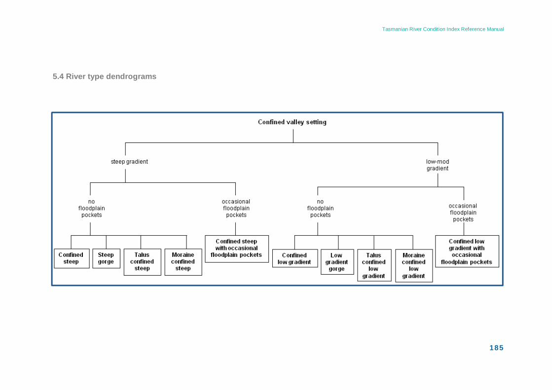
Tasmanian River Condition Index Reference Manual
185
5.4 River type dendrograms
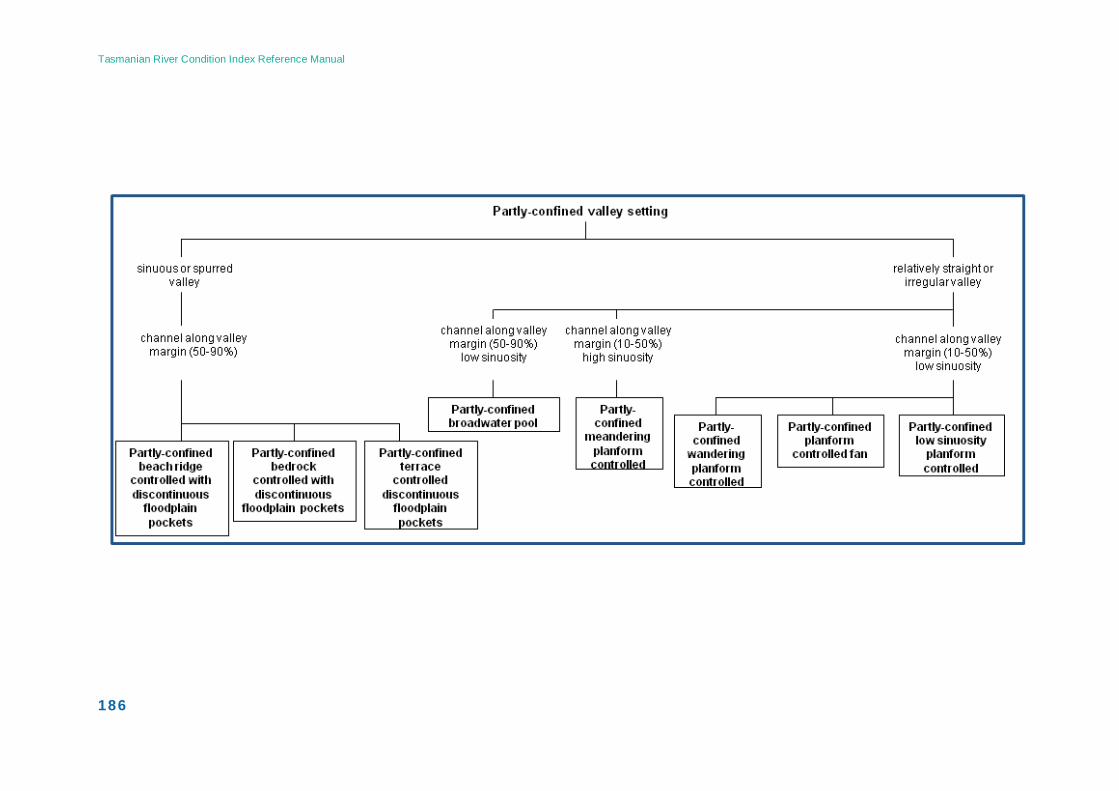
Tasmanian River Condition Index Reference Manual
186
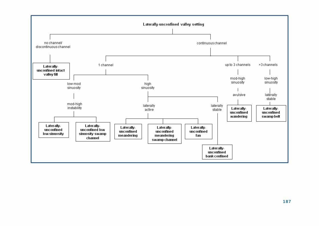
Tasmanian River Condition Index Reference Manual
187
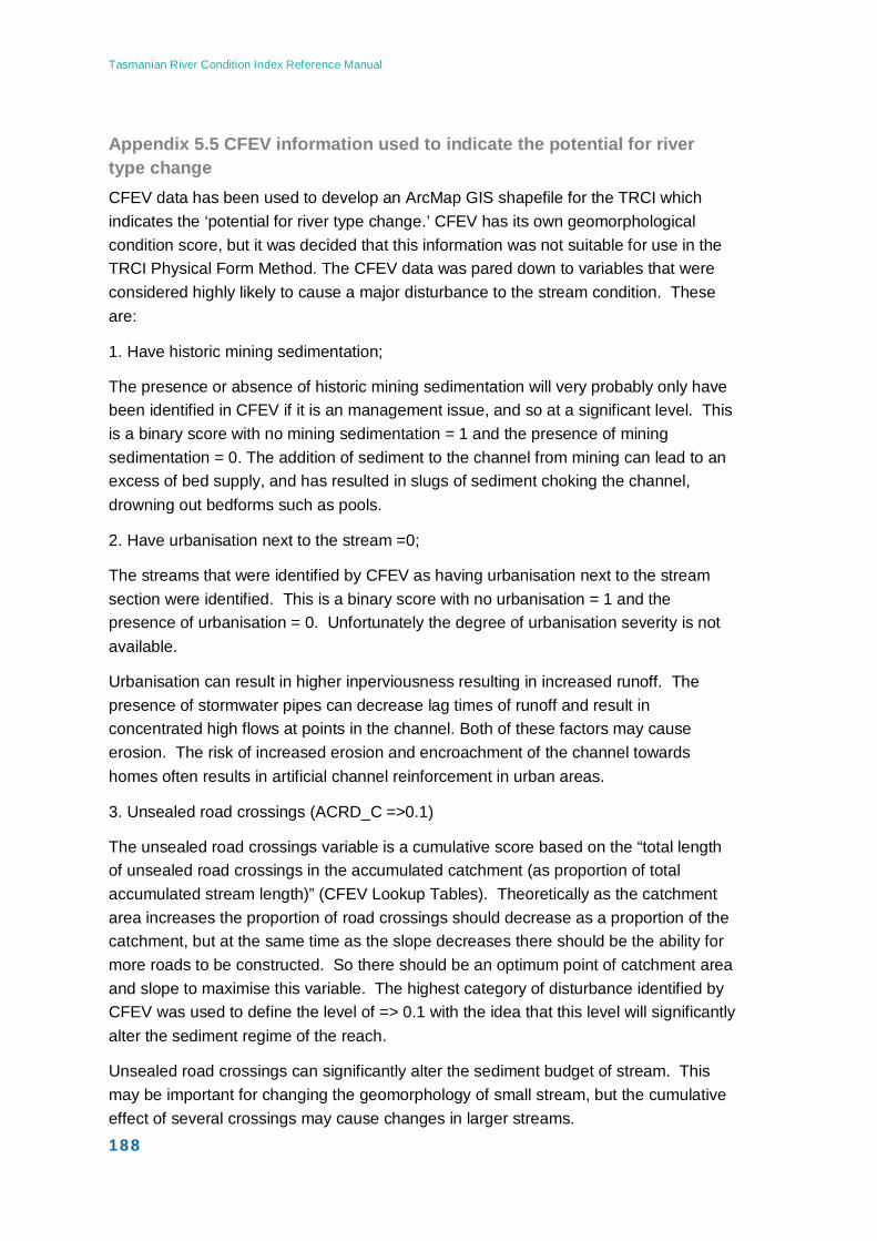
Tasmanian River Condition Index Reference Manual
188
Appendix 5.5 CFEV information used to indicate the potential for river type change CFEV data has been used to develop an ArcMap GIS shapefile for the TRCI which indicates the ‘potential for river type change.’ CFEV has its own geomorphological condition score, but it was decided that this information was not suitable for use in the TRCI Physical Form Method. The CFEV data was pared down to variables that were considered highly likely to cause a major disturbance to the stream condition. These are:
1. Have historic mining sedimentation;
The presence or absence of historic mining sedimentation will very probably only have been identified in CFEV if it is an management issue, and so at a significant level. This is a binary score with no mining sedimentation = 1 and the presence of mining sedimentation = 0. The addition of sediment to the channel from mining can lead to an excess of bed supply, and has resulted in slugs of sediment choking the channel, drowning out bedforms such as pools.
2. Have urbanisation next to the stream =0;
The streams that were identified by CFEV as having urbanisation next to the stream section were identified. This is a binary score with no urbanisation = 1 and the presence of urbanisation = 0. Unfortunately the degree of urbanisation severity is not available.
Urbanisation can result in higher inperviousness resulting in increased runoff. The presence of stormwater pipes can decrease lag times of runoff and result in concentrated high flows at points in the channel. Both of these factors may cause erosion. The risk of increased erosion and encroachment of the channel towards homes often results in artificial channel reinforcement in urban areas.
3. Unsealed road crossings (ACRD_C =>0.1)
The unsealed road crossings variable is a cumulative score based on the “total length of unsealed road crossings in the accumulated catchment (as proportion of total accumulated stream length)” (CFEV Lookup Tables). Theoretically as the catchment area increases the proportion of road crossings should decrease as a proportion of the catchment, but at the same time as the slope decreases there should be the ability for more roads to be constructed. So there should be an optimum point of catchment area and slope to maximise this variable. The highest category of disturbance identified by CFEV was used to define the level of => 0.1 with the idea that this level will significantly alter the sediment regime of the reach.
Unsealed road crossings can significantly alter the sediment budget of stream. This may be important for changing the geomorphology of small stream, but the cumulative effect of several crossings may cause changes in larger streams.
Tasmanian River Condition Index Reference Manual
189
4. Catchment disturbance – 90% (CATID <= 0.1)
This is again a cumulative variable showing the “Upstream accumulated catchment disturbance score for the river section” (CFEV Lookup Tables). As the catchment gets larger the amount of disturbance would have to be larger, and thus there should again be an optimum level at which the slopes in the catchment are suitable for disturbance and the catchment size relative to disturbance size (i.e. forestry operations) are maximised.
The variable CATID was used rather than CATID_C. This is most basic, or rawest, information available in CFEV rather than using something that has been manipulated into a categorical score. CFEV uses a worst case value of 0.05 or 95% of the catchment disturbed, which is possibly based around the distribution of the data. Looking at the distribution of impacted sites it was decided that 0.1 or 90% of the catchment being disturbed was a more appropriate level for known disturbances.
Catchment disturbance is a change in the landuse away from its natural condition. These changes can result in differences in the evaporation, evapotranspiration, and interception of the area, which may then alter the runoff and associated sediment. Increased or decreased volumes of water in the channel, along with changed lag times and sediment concentrations may result in a change in the geomorphology of the stream.
5. Hydrology disturbance is high – (FLOW <=0.3)
The CFEV Lookup Tables suggest that this level indicates a very large change to flow regime for the river section. * Note that this attribute ranges continuously between 1 ('best case' or equivalent to natural) and 0 ('worst case' ie very altered from natural) without distinct internal thresholds in condition, and that these descriptors and ranges are provided for guidance only, that is, there are no sharp boundaries between condition descriptor states. A major change in the hydrology of a stream will alter the sediment regime and result in geomorphic change.
With all these remotely sensed variables it is difficult to know where the threshold value should be drawn. It is a subjective method and unfortunately only extensive field testing will allow the levels to be fine-tuned to allow slightly more accuracy.
Using CFEV within ArcMap the following script identifies reaches that have one or more of the above variables. The first part of the script selects true stream segments (not those that are theoretical flow routes), and streams that are greater than 1st order.
"RS_ORDER" > 1 AND "RS_ACID" < 999 AND "RS_PIPE" =0 AND ( "RS_FLOW" <=0.3 OR "RS_ACRD_U" >= 0.1 OR "RS_URBAN" = 0 OR "RS_MINES" = 0 OR "RS_CATDI" <= 0.1)
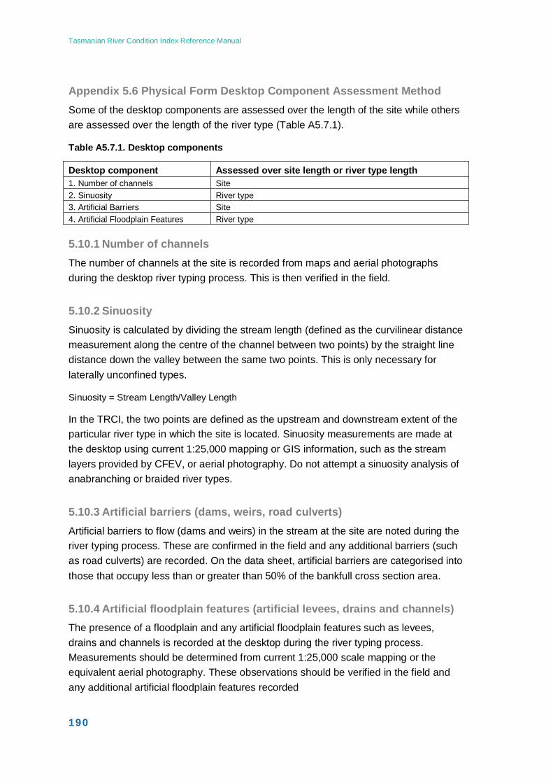
Tasmanian River Condition Index Reference Manual
190
Appendix 5.6 Physical Form Desktop Component Assessment Method Some of the desktop components are assessed over the length of the site while others are assessed over the length of the river type (Table A5.7.1).
Table A5.7.1. Desktop components
Desktop component Assessed over site length or river type length 1. Number of channels Site 2. Sinuosity River type 3. Artificial Barriers Site 4. Artificial Floodplain Features River type
5.10.1 Number of channels The number of channels at the site is recorded from maps and aerial photographs during the desktop river typing process. This is then verified in the field.
5.10.2 Sinuosity Sinuosity is calculated by dividing the stream length (defined as the curvilinear distance measurement along the centre of the channel between two points) by the straight line distance down the valley between the same two points. This is only necessary for laterally unconfined types.
Sinuosity = Stream Length/Valley Length
In the TRCI, the two points are defined as the upstream and downstream extent of the particular river type in which the site is located. Sinuosity measurements are made at the desktop using current 1:25,000 mapping or GIS information, such as the stream layers provided by CFEV, or aerial photography. Do not attempt a sinuosity analysis of anabranching or braided river types.
5.10.3 Artificial barriers (dams, weirs, road culverts) Artificial barriers to flow (dams and weirs) in the stream at the site are noted during the river typing process. These are confirmed in the field and any additional barriers (such as road culverts) are recorded. On the data sheet, artificial barriers are categorised into those that occupy less than or greater than 50% of the bankfull cross section area.
5.10.4 Artificial floodplain features (artificial levees, drains and channels) The presence of a floodplain and any artificial floodplain features such as levees, drains and channels is recorded at the desktop during the river typing process. Measurements should be determined from current 1:25,000 scale mapping or the equivalent aerial photography. These observations should be verified in the field and any additional artificial floodplain features recorded

Tasmanian River Condition Index Reference Manual
191

Tasmanian River Condition Index Reference Manual
192
5.10.5 Appendix 5.6 Physical Form Data Sheet This datasheet is also available from NRM South as a separate file.
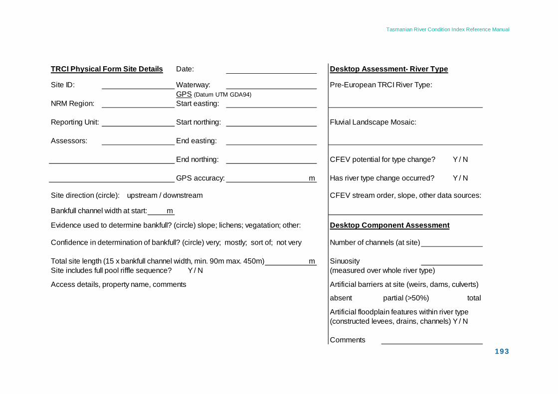
Tasmanian River Condition Index Reference Manual
193
TRCI Physical Form Site Details Date: Desktop Assessment- River Type
Site ID: Waterway: Pre-European TRCI River Type:GPS (Datum UTM GDA94)
NRM Region: Start easting:
Reporting Unit: Start northing: Fluvial Landscape Mosaic:
Assessors: End easting:
End northing: CFEV potential for type change? Y / N
GPS accuracy: m Has river type change occurred? Y / N
Site direction (circle): upstream / downstream CFEV stream order, slope, other data sources:
Bankfull channel width at start: m
Evidence used to determine bankfull? (circle) slope; lichens; vegatation; other: Desktop Component Assessment
Confidence in determination of bankfull? (circle) very; mostly; sort of; not very Number of channels (at site)
Total site length (15 x bankfull channel width, min. 90m max. 450m) m Sinuosity Site includes full pool riffle sequence? Y / N (measured over whole river type)
Access details, property name, comments Artificial barriers at site (weirs, dams, culverts)
absent partial (>50%) total
Artificial floodplain features within river type(constructed levees, drains, channels) Y / N
Comments
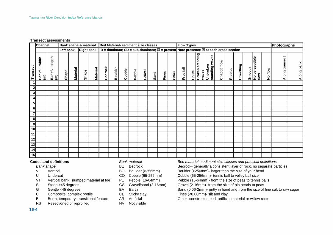
Tasmanian River Condition Index Reference Manual
194
Transect assessmentsPhotographs
Ban
kful
l wid
th
(m)
Ban
kful
l dep
th
(m)
Shap
e
Mat
eria
l
Shap
e
Mat
eria
l
Bed
rock
Bou
lder
Cob
ble
Pebb
le
Gra
vel
Sand
Fine
s
Oth
er
Free
fall
Chu
teB
roke
n st
andi
ng
wav
esU
nbro
ken
stan
ding
wav
es
Cha
otic
flow
Rip
pled
Upw
ellin
g
Smoo
thN
o pe
rcep
tible
flo
w
No
flow
Alo
ng tr
anse
ct
Alo
ng b
ank
123456789
101112131415
Codes and definitions Bank material Bed material- sediment size classes and practical definitionsBank shape BE Bedrock Bedrock- generally a consistent layer of rock, no separate particlesV Vertical BO Boulder (>256mm) Boulder (>256mm)- larger than the size of your headU Undercut CO Cobble (65-256mm) Cobble (65-256mm)- tennis ball to volley ball sizeVT Vertical bank, slumped material at toe PE Pebble (16-64mm) Pebble (16-64mm)- from the size of peas to tennis ballsS Steep >45 degrees GS Gravel/sand (2-16mm) Gravel (2-16mm)- from the size of pin heads to peasG Gentle <45 degrees EA Earth Sand (0.06-2mm)- gritty in hand and from the size of fine salt to raw sugarC Composite, complex profile CL Sticky clay Fines (<0.06mm)- silt and clayB Berm, temporary, transitional feature AR Artificial Other- constructed bed, artificial material or willow rootsRS Resectioned or reprofiled NV Not visible
Note presence at each cross section
Tran
sect
Channel Bank shape & material Bed Material- sediment size classes Flow TypesLeft bank Right bank D = dominant; SD = sub-dominant; = present
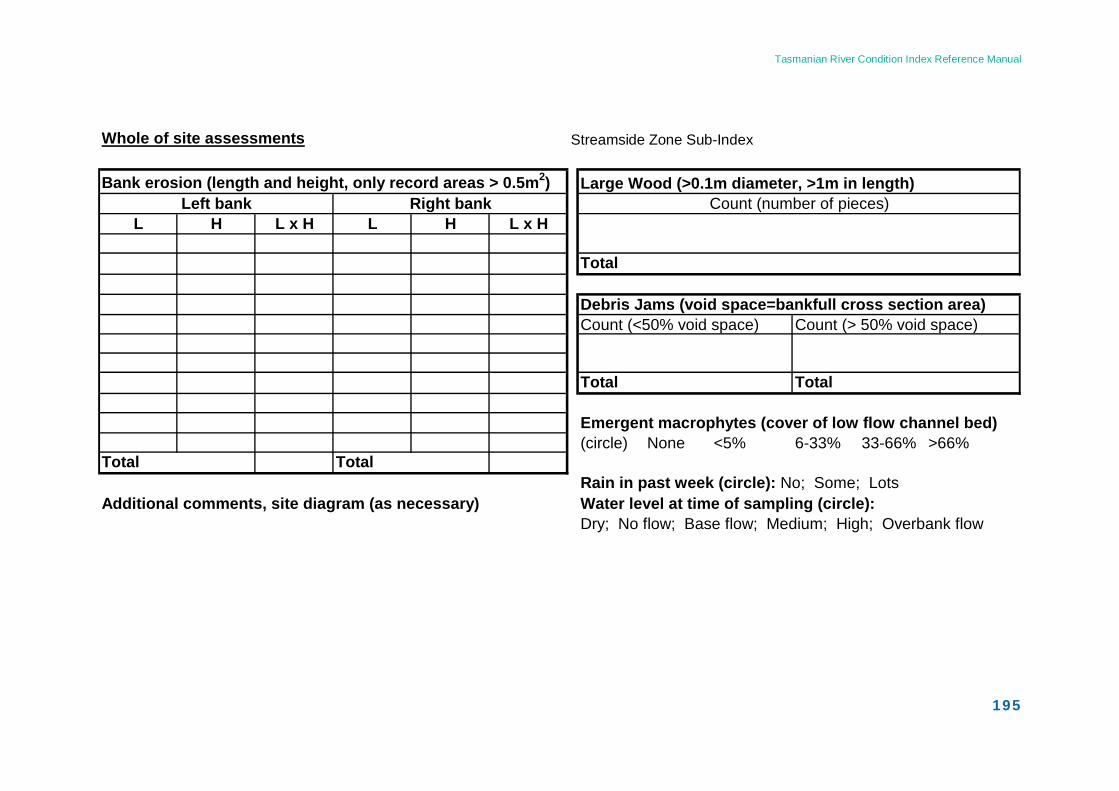
Tasmanian River Condition Index Reference Manual
195
Whole of site assessments
Bank erosion (length and height, only record areas > 0.5m2)
L H L x H L H L x H
Debris Jams (void space=bankfull cross section area)Count (<50% void space) Count (> 50% void space)
Emergent macrophytes (cover of low flow channel bed) (circle) None <5% 6-33% 33-66% >66%
Rain in past week (circle): No; Some; LotsAdditional comments, site diagram (as necessary) Water level at time of sampling (circle):
Dry; No flow; Base flow; Medium; High; Overbank flow
Large Wood (>0.1m diameter, >1m in length)
Total Total
Count (number of pieces)
Total
Total Total
Left bank Right bank
Streamside Zone Sub-Index

Tasmanian River Condition Index Reference Manual
196
Tasmanian River Condition Index Reference Manual
197
6 Streamside Zone Sub-Index The objective of the Streamside Zone sub-index is to provide a measure of the condition of riparian vegetation and habitat values adjacent to the waterway. The components assessed within this sub-index contribute directly and indirectly to the condition of the waterway.
The Streamside Zone sub-index uses a referential approach to measure the condition of riparian vegetation relative to its pre-1750 state. This pre-1750 state is defined by a set of benchmarks for the different riparian vegetation communities found in Tasmania. These benchmarks were developed specifically for the Tasmanian River Condition Index. Riparian vegetation in Tasmania varies widely in structure and composition. For the purposes of measuring condition, riparian vegetation communities in Tasmania were divided into two groups: woody and non-woody, with the woody communities further sub-divided into forest/woodland communities and shrubby communities, depending on the size of the dominant woody species.
The Streamside Zone sub-index includes 13 components, three of which are assessed using a geographical information system (GIS), while the others are assessed in the field. While the raw data for all components are recorded in the field, not all components are scored in all vegetation communities, e.g. tree cover and large trees are only scored in forest/woodland communities, while recruitment of woody species and logs are not scored in non-woody communities. Scores are calculated for each site by comparing observed values for each component to benchmark values specified for the vegetation type (in some cases these benchmarks are the same for all vegetation types, e.g. the weed cover benchmark is zero in all cases). In all cases a zero score for a component indicates poorest condition while the maximum score indicates best condition.
This chapter first describes the background to the development of the Streamside Zone sub-index method, showing what components were chosen as indicators of condition and why they were chosen. The referential approach is then described in more detail, with information on the development of benchmarks for different riparian vegetation communities. This is followed by a detailed description of each of the components which make up the Streamside Zone sub-index. The remainder of the chapter details the methods use to collect the field data and score the components to derive a final Streamside Zone sub-index score.
6.1 Background, component selection and rationale Existing methods for river and vegetation condition assessment were examined for suitability for use in the Streamside Zone sub-index of the Tasmanian River Condition Index (TRCI). These included the Rapid Appraisal of Riparian Condition (Jansen et al.
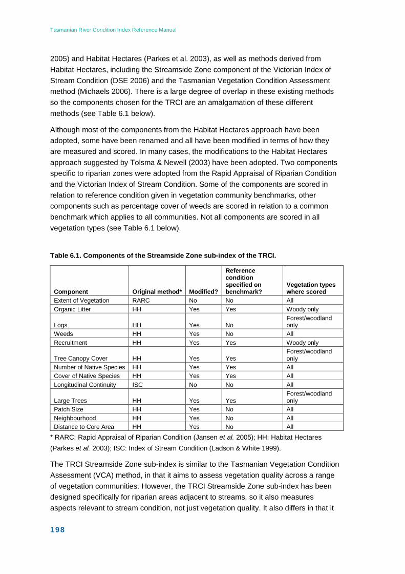
Tasmanian River Condition Index Reference Manual
198
2005) and Habitat Hectares (Parkes et al. 2003), as well as methods derived from Habitat Hectares, including the Streamside Zone component of the Victorian Index of Stream Condition (DSE 2006) and the Tasmanian Vegetation Condition Assessment method (Michaels 2006). There is a large degree of overlap in these existing methods so the components chosen for the TRCI are an amalgamation of these different methods (see Table 6.1 below).
Although most of the components from the Habitat Hectares approach have been adopted, some have been renamed and all have been modified in terms of how they are measured and scored. In many cases, the modifications to the Habitat Hectares approach suggested by Tolsma & Newell (2003) have been adopted. Two components specific to riparian zones were adopted from the Rapid Appraisal of Riparian Condition and the Victorian Index of Stream Condition. Some of the components are scored in relation to reference condition given in vegetation community benchmarks, other components such as percentage cover of weeds are scored in relation to a common benchmark which applies to all communities. Not all components are scored in all vegetation types (see Table 6.1 below).
Table 6.1. Components of the Streamside Zone sub-index of the TRCI.
Component Original method* Modified?
Reference condition specified on benchmark?
Vegetation types where scored
Extent of Vegetation RARC No No All Organic Litter HH Yes Yes Woody only
Logs HH Yes No Forest/woodland only
Weeds HH Yes No All Recruitment HH Yes Yes Woody only
Tree Canopy Cover HH Yes Yes Forest/woodland only
Number of Native Species HH Yes Yes All Cover of Native Species HH Yes Yes All Longitudinal Continuity ISC No No All
Large Trees HH Yes Yes Forest/woodland only
Patch Size HH Yes No All Neighbourhood HH Yes No All Distance to Core Area HH Yes No All
* RARC: Rapid Appraisal of Riparian Condition (Jansen et al. 2005); HH: Habitat Hectares (Parkes et al. 2003); ISC: Index of Stream Condition (Ladson & White 1999).
The TRCI Streamside Zone sub-index is similar to the Tasmanian Vegetation Condition Assessment (VCA) method, in that it aims to assess vegetation quality across a range of vegetation communities. However, the TRCI Streamside Zone sub-index has been designed specifically for riparian areas adjacent to streams, so it also measures aspects relevant to stream condition, not just vegetation quality. It also differs in that it
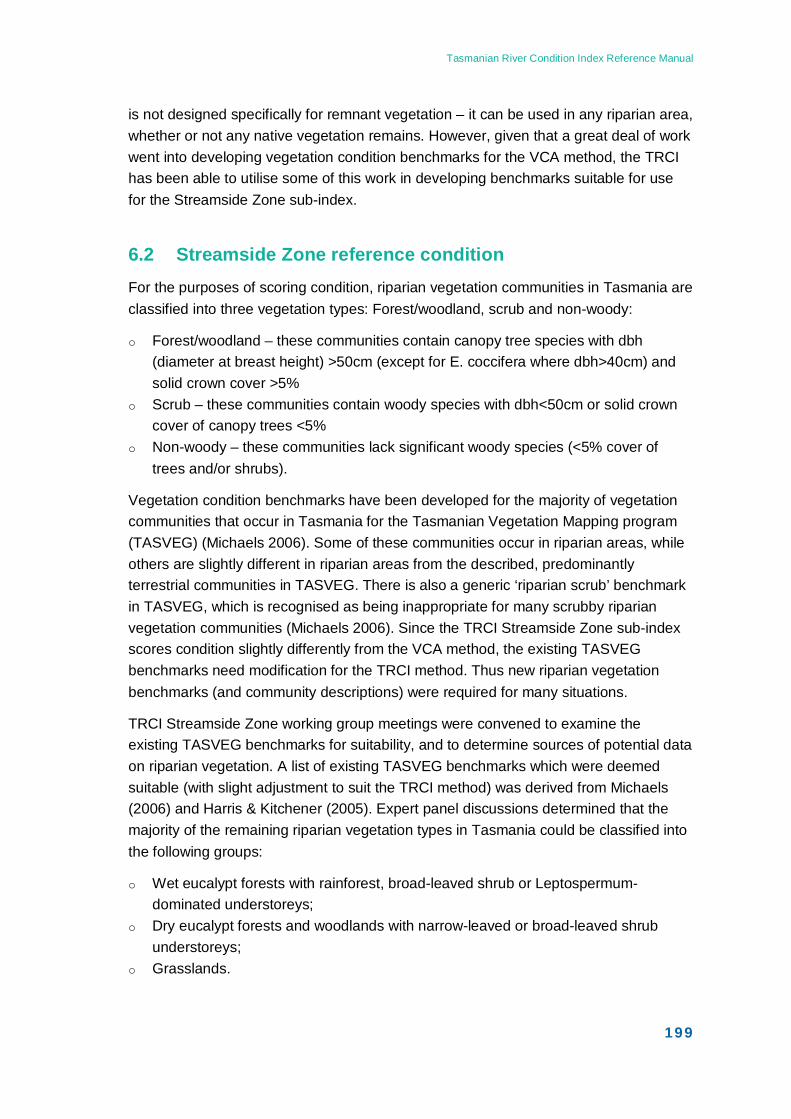
Tasmanian River Condition Index Reference Manual
199
is not designed specifically for remnant vegetation – it can be used in any riparian area, whether or not any native vegetation remains. However, given that a great deal of work went into developing vegetation condition benchmarks for the VCA method, the TRCI has been able to utilise some of this work in developing benchmarks suitable for use for the Streamside Zone sub-index.
6.2 Streamside Zone reference condition For the purposes of scoring condition, riparian vegetation communities in Tasmania are classified into three vegetation types: Forest/woodland, scrub and non-woody:
o Forest/woodland – these communities contain canopy tree species with dbh (diameter at breast height) >50cm (except for E. coccifera where dbh>40cm) and solid crown cover >5%
o Scrub – these communities contain woody species with dbh<50cm or solid crown cover of canopy trees <5%
o Non-woody – these communities lack significant woody species (<5% cover of trees and/or shrubs).
Vegetation condition benchmarks have been developed for the majority of vegetation communities that occur in Tasmania for the Tasmanian Vegetation Mapping program (TASVEG) (Michaels 2006). Some of these communities occur in riparian areas, while others are slightly different in riparian areas from the described, predominantly terrestrial communities in TASVEG. There is also a generic ‘riparian scrub’ benchmark in TASVEG, which is recognised as being inappropriate for many scrubby riparian vegetation communities (Michaels 2006). Since the TRCI Streamside Zone sub-index scores condition slightly differently from the VCA method, the existing TASVEG benchmarks need modification for the TRCI method. Thus new riparian vegetation benchmarks (and community descriptions) were required for many situations.
TRCI Streamside Zone working group meetings were convened to examine the existing TASVEG benchmarks for suitability, and to determine sources of potential data on riparian vegetation. A list of existing TASVEG benchmarks which were deemed suitable (with slight adjustment to suit the TRCI method) was derived from Michaels (2006) and Harris & Kitchener (2005). Expert panel discussions determined that the majority of the remaining riparian vegetation types in Tasmania could be classified into the following groups:
o Wet eucalypt forests with rainforest, broad-leaved shrub or Leptospermum-dominated understoreys;
o Dry eucalypt forests and woodlands with narrow-leaved or broad-leaved shrub understoreys;
o Grasslands.

Tasmanian River Condition Index Reference Manual
200
Floristic data from Askey-Doran (1993) were used to confirm these riparian communities, and to derive benchmark values for these generic communities for TRCI condition assessment. Further details of the development of riparian vegetation benchmarks can be found in Appendix 6.
The list of riparian vegetation communities for which benchmarks were adapted or developed is shown in Table 6.2. The TASVEG benchmarks used in the TRCI with minor modification have retained their names and codes, while the ones developed specifically for riparian communities have “TRCI’ codes. Note that benchmarks have not yet been developed for three communities because of a lack of data. Eventually it is hoped that benchmarks will be developed for these communities, so that sites with these vegetation communities can be scored correctly. Details of the benchmark values for all of the riparian vegetation communities can be found in Appendix 6. Descriptions of these communities, and a key to their identification, can also be found in the Appendix.
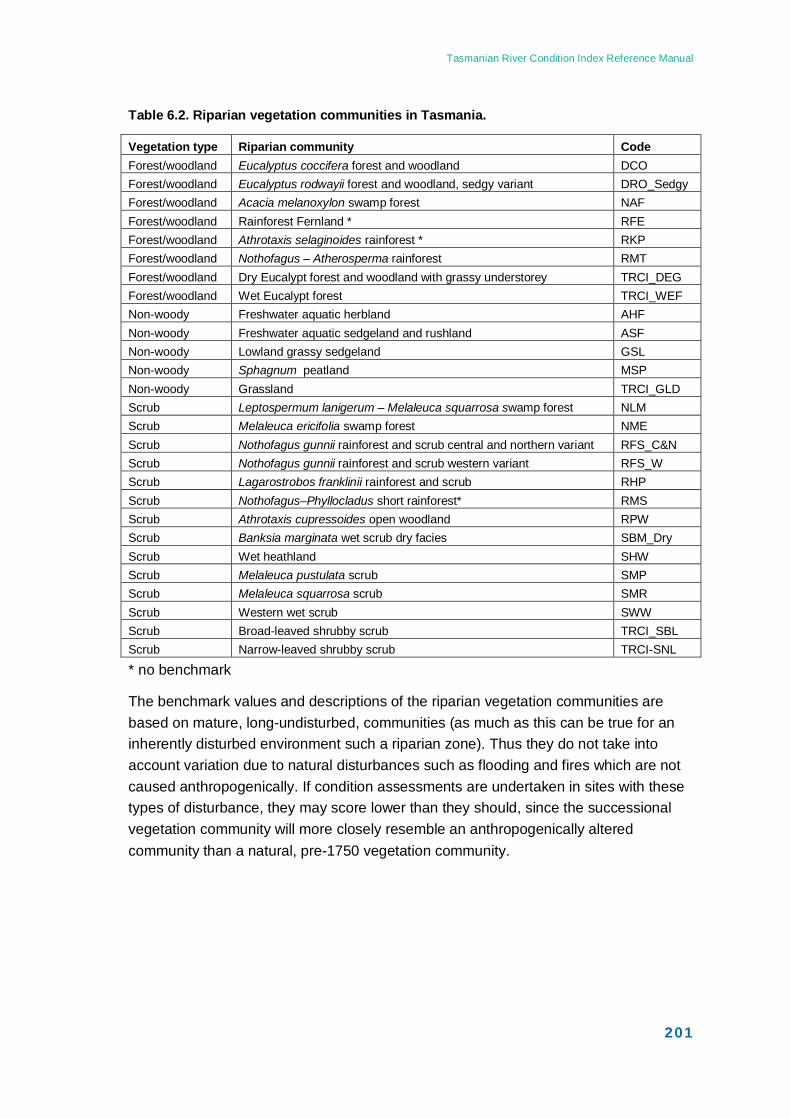
Tasmanian River Condition Index Reference Manual
201
Table 6.2. Riparian vegetation communities in Tasmania.
Vegetation type Riparian community Code Forest/woodland Eucalyptus coccifera forest and woodland DCO Forest/woodland Eucalyptus rodwayii forest and woodland, sedgy variant DRO_Sedgy Forest/woodland Acacia melanoxylon swamp forest NAF Forest/woodland Rainforest Fernland * RFE Forest/woodland Athrotaxis selaginoides rainforest * RKP Forest/woodland Nothofagus – Atherosperma rainforest RMT Forest/woodland Dry Eucalypt forest and woodland with grassy understorey TRCI_DEG Forest/woodland Wet Eucalypt forest TRCI_WEF Non-woody Freshwater aquatic herbland AHF Non-woody Freshwater aquatic sedgeland and rushland ASF Non-woody Lowland grassy sedgeland GSL Non-woody Sphagnum peatland MSP Non-woody Grassland TRCI_GLD Scrub Leptospermum lanigerum – Melaleuca squarrosa swamp forest NLM Scrub Melaleuca ericifolia swamp forest NME Scrub Nothofagus gunnii rainforest and scrub central and northern variant RFS_C&N Scrub Nothofagus gunnii rainforest and scrub western variant RFS_W Scrub Lagarostrobos franklinii rainforest and scrub RHP Scrub Nothofagus–Phyllocladus short rainforest* RMS Scrub Athrotaxis cupressoides open woodland RPW Scrub Banksia marginata wet scrub dry facies SBM_Dry Scrub Wet heathland SHW Scrub Melaleuca pustulata scrub SMP Scrub Melaleuca squarrosa scrub SMR Scrub Western wet scrub SWW Scrub Broad-leaved shrubby scrub TRCI_SBL Scrub Narrow-leaved shrubby scrub TRCI-SNL
* no benchmark
The benchmark values and descriptions of the riparian vegetation communities are based on mature, long-undisturbed, communities (as much as this can be true for an inherently disturbed environment such a riparian zone). Thus they do not take into account variation due to natural disturbances such as flooding and fires which are not caused anthropogenically. If condition assessments are undertaken in sites with these types of disturbance, they may score lower than they should, since the successional vegetation community will more closely resemble an anthropogenically altered community than a natural, pre-1750 vegetation community.
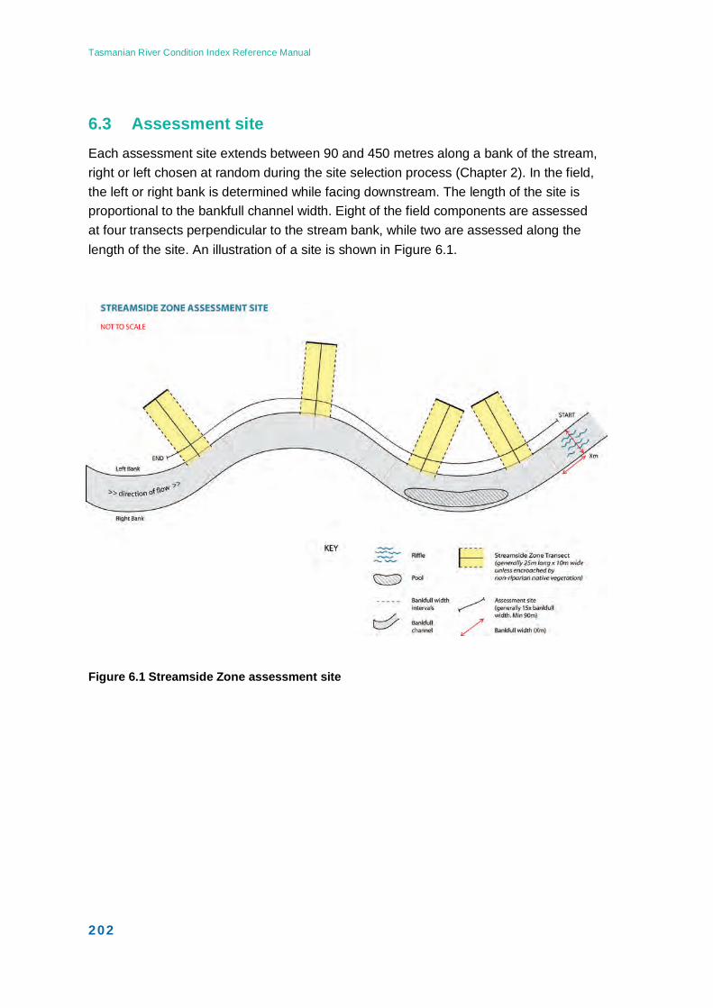
Tasmanian River Condition Index Reference Manual
202
6.3 Assessment site Each assessment site extends between 90 and 450 metres along a bank of the stream, right or left chosen at random during the site selection process (Chapter 2). In the field, the left or right bank is determined while facing downstream. The length of the site is proportional to the bankfull channel width. Eight of the field components are assessed at four transects perpendicular to the stream bank, while two are assessed along the length of the site. An illustration of a site is shown in Figure 6.1.
Figure 6.1 Streamside Zone assessment site
Tasmanian River Condition Index Reference Manual
203
6.4 Description of components
6.4.1 Extent of vegetation (EV) The width of vegetation adjacent to the stream is important as it forms a buffer to external impacts on the stream, as well as providing physical stability and ecological benefits. In the TRCI, the width of streamside vegetation is related to the stream channel size as large streams potentially require broad buffers, particularly from a stability perspective. Larger streams are often within alluvial lowland floodplains that are more susceptible to natural or accelerated bank migration. The maximum score is assigned to small streams (≤10 metres wide), where the extent of vegetation exceeds 40m, or large streams (>10 metres wide) where the extent of vegetation is at least four times the channel width. A score of zero is assigned where the extent of vegetation is <5 m on small streams, or less than half of the channel width in large streams.
6.4.2 Organic litter (OL) Appropriate levels of organic litter provide important terrestrial and aquatic ecological benefits. This component involves recording the percentage cover of organic litter (any dead plant material which is detached from the parent plant and is <10cm in diameter) in each transect and averaging across transects. The observed cover of organic litter at the site is compared with the benchmark for organic litter in that vegetation community.
6.4.3 Logs (LG) Logs provide important habitat and contribute to the ecological functioning of ecosystems. Plants and animals may use logs as a substrate for germination and growth, feeding, perching or residence. The organisms that reside on, under, or in logs, may be involved in nitrogen fixation, nutrient cycling and mycorrhizal fungal associations. Given the paucity of knowledge about expected amounts of logs found in different riparian communities within Tasmania, this component currently does not have a reference condition for different vegetation types and is only scored within woody vegetation types. The total length of all logs (>10cm diameter) in each transect is recorded (to a maximum of 40 m per transect) and summed across transects. It is scored on a simple three-point scale.
6.4.4 Weeds (WD) The presence of weeds is considered an indicator of disturbance and a threat to the condition and viability of native vegetation. Weeds can also reduce stream condition directly (i.e. shade, leaf drop, physical encroachment). The cover of high threat weeds (see below) only is used in scoring this component. The cover of all weeds is also recorded in the field but this information does not contribute to the scoring for this

Tasmanian River Condition Index Reference Manual
204
component. It should be noted that the TRCI does not use the definition of high threat weeds specified in the VCA method. This definition, in which a high threat weed is any species which offers >5% cover, is not appropriate in riparian or disturbed environments where ubiquitous or pasture species may be relatively common. These species may not be a high priority for natural resource management.
The TRCI High Threat Weeds list has been compiled with the assistance of the DPIW Weeds Section. Weeds on the list are Weeds of National Significance (WONS), declared weeds in Tasmania, ecologically threatening weeds (not declared) and new and emerging weeds based on invasiveness, impact and threat to riparian environments. It is envisaged that the list could be updated in the future as new weed threats emerge. The full list can be found in Appendix 6.
Weeds are divided into tree, shrub and ground lifeforms, based on height and woodiness (trees – woody, >2m, shrubs – woody, <2m, ground – non-woody) and cover classes based on projective foliage cover are recorded in the field, both for all weeds, and for high threat weeds only. Scores are assigned for each cover class for each lifeform in each transect. These are then averaged across the transects to give a score for each lifeform at the site. Lifeform scores are then summed to give a total score for the site.
6.4.5 Recruitment (RC) Natural regeneration is vital to the sustainability of a vegetation community and is therefore considered an important component of stream condition. For this component the presence of recruitment of woody species is recorded. Due to low observer reliability with the Habitat Hectares method (Tolsma & Newell 2003), and lack of applicability to riparian situations, the scoring for this component has been significantly altered from that found in the Habitat Hectares method.
In the current method, the number of woody species with recruitment is recorded over the whole site. A recruit is defined as a non-fruiting, non-budding individual that is relatively established, i.e. approximately greater than 1 year old. The number of species recruiting is compared with the benchmark number of species recruiting. This component is not scored in non-woody vegetation communities.
6.4.6 Tree canopy cover (TC) This measure indicates the cover of the upper most stratum within the vegetation community and is only scored for forest/woodland vegetation types. In the Habitat Hectares method tree canopy health was also assessed, but it has been eliminated from the TRCI method due to subjectivity of assessment and redundancy (Tolsma and Newell 2003). The projective foliage cover of the tree canopy species is estimated at each transect. Tree canopy species include those trees which form part of the canopy and are at least 80% of mature tree height for that vegetation community. The values
Tasmanian River Condition Index Reference Manual
205
for tree canopy cover in transects are averaged, and then compared to the benchmark tree canopy cover.
6.4.7 Number of native species (SP) The diversity of species within the riparian vegetation community provides information about the integrity of the community, as well as its ability to provide resources to a wide range of other organisms. This component is a modification of the ’Understorey Lifeforms’ component of the Habitat Hectares method. Diversity and structure have been separated in the TRCI method, to avoid confounding these two aspects and to simplify measurement. ‘Number of native species’ assesses diversity, whereas ‘Cover of native species’ assesses structure. The total number of species observed across all transects is recorded and compared to the benchmark number for the vegetation community.
6.4.8 Cover of native species (CO) The cover of each lifeform provides a measure of the structural integrity of the riparian vegetation, as well as providing information about habitat complexity, which is important for riparian fauna. This component measures the foliage projective cover of each lifeform in each transect. These values are then averaged across transects. The list of lifeforms used (see Appendix 6) has been simplified from that used in the Habitat Hectares method, to avoid inter-observer differences which were reported in Tolsma and Newell (2003). For each lifeform (except mature tree canopy cover which is used for the ‘Tree canopy cover’ score – see above) the observed cover is compared to the benchmark cover.
6.4.9 Longitudinal continuity (LC) Longitudinal continuity is a measure of the degree to which vegetation is continuous along a waterway. A continuous strip of riparian vegetation has important physical and ecological functions and is fundamental to stream condition. The continuity of vegetation is important for bank stability, terrestrial fauna passage, provision of shade and other inputs to the stream. It is assessed as in the Victorian ISC method (Ladson & White 1999), although for non-woody vegetation types, it is modified so that only native vegetation is included (for woody vegetation communities, continuous vegetation includes all woody species, regardless of origin). The assessment for this component involves recording the length of continuous vegetation and the length of ‘breaks’ in vegetation along the stream. To be recorded as ‘continuous,’ woody vegetation must provide >50% solid crown cover, and be ≥5m wide (from the toe of the bank extending offstream), and ≥10 metres in length. Exotic vegetation such as willows, gorse and blackberry can contribute towards ‘continuity’ if they satisfy the cover, length and width criteria. In non-woody vegetation types (e.g. grasslands or moorlands with little or no woody vegetation present), vegetation cover will be deemed present if the native
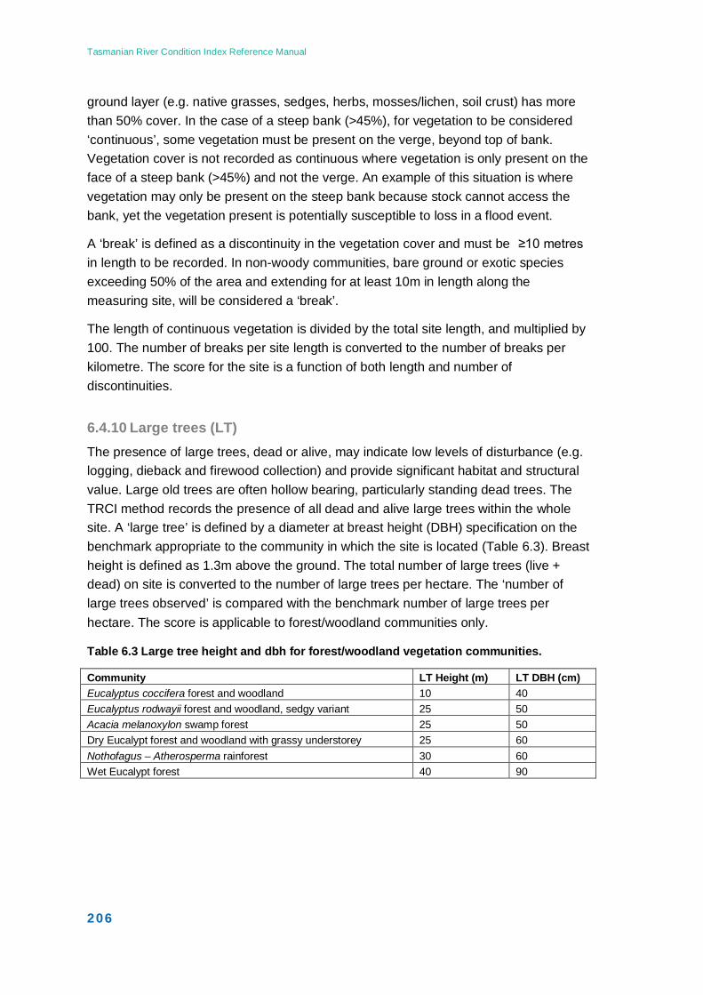
Tasmanian River Condition Index Reference Manual
206
ground layer (e.g. native grasses, sedges, herbs, mosses/lichen, soil crust) has more than 50% cover. In the case of a steep bank (>45%), for vegetation to be considered ‘continuous’, some vegetation must be present on the verge, beyond top of bank. Vegetation cover is not recorded as continuous where vegetation is only present on the face of a steep bank (>45%) and not the verge. An example of this situation is where vegetation may only be present on the steep bank because stock cannot access the bank, yet the vegetation present is potentially susceptible to loss in a flood event.
A ‘break’ is defined as a discontinuity in the vegetation cover and must be ≥10 metres in length to be recorded. In non-woody communities, bare ground or exotic species exceeding 50% of the area and extending for at least 10m in length along the measuring site, will be considered a ‘break’.
The length of continuous vegetation is divided by the total site length, and multiplied by 100. The number of breaks per site length is converted to the number of breaks per kilometre. The score for the site is a function of both length and number of discontinuities.
6.4.10 Large trees (LT) The presence of large trees, dead or alive, may indicate low levels of disturbance (e.g. logging, dieback and firewood collection) and provide significant habitat and structural value. Large old trees are often hollow bearing, particularly standing dead trees. The TRCI method records the presence of all dead and alive large trees within the whole site. A ‘large tree’ is defined by a diameter at breast height (DBH) specification on the benchmark appropriate to the community in which the site is located (Table 6.3). Breast height is defined as 1.3m above the ground. The total number of large trees (live + dead) on site is converted to the number of large trees per hectare. The ‘number of large trees observed’ is compared with the benchmark number of large trees per hectare. The score is applicable to forest/woodland communities only.
Table 6.3 Large tree height and dbh for forest/woodland vegetation communities.
Community LT Height (m) LT DBH (cm) Eucalyptus coccifera forest and woodland 10 40 Eucalyptus rodwayii forest and woodland, sedgy variant 25 50 Acacia melanoxylon swamp forest 25 50 Dry Eucalypt forest and woodland with grassy understorey 25 60 Nothofagus – Atherosperma rainforest 30 60 Wet Eucalypt forest 40 90

Tasmanian River Condition Index Reference Manual
207
6.4.11 Patch size (PS) The size of a patch of remnant vegetation contributes to its long-term viability. In general, larger patches have a greater survival rate as they support more species, populations, retain greater genetic variability and provide refuge for species susceptible to disturbances. ‘Edge effects’ such as weed invasion, may contribute to the demise of small native vegetation fragments (Parkes et al. 2003).
This method has been modified slightly from that used in the Habitat Hectares approach as suggested by Tolsma and Newell (2003). The area of the patch of native vegetation in which the site is located is recorded and scored as in the Habitat Hectares approach. However, the score is not qualified by whether the patch is significantly disturbed. This change also applies to the ‘Neighbourhood’ and ‘Distance to Core Area’ components. A relatively rapid GIS process to calculate this component has been developed. This process uses TASVEG mapping to identify whether the site is located in an area of native vegetation, and if so, the size of that patch of native vegetation. The final score is derived by multiplying the patch size (ha) by 25, as recommended in Tolsma and Newell (2003).
6.4.12 Neighbourhood (NB) The neighbourhood score measures the amount and configuration of native vegetation around the site being assessed. This component is assessed using a GIS, but may require some checking in the field. Native vegetation includes any vegetation community regardless of type, condition or tenure and can also include natural wetlands, lakes (i.e. not artificial impoundments), estuaries and rivers. When assessing near coastal vegetation, the shape of the neighbourhood boundaries should be adjusted to coincide with the low tide mark thus excluding the open sea/ocean. If the community is a native grassland or pasture, assessors should make field observations to confirm GIS/TASVEG results, as TASVEG may not differentiate between the extent of native and exotic grassland/pasture communities.
The assessment method involves drawing three concentric circles (100m, 1 km and 5km radii) around the measuring site, centred upon the start co-ordinate of the site. The percentage of native vegetation in each circle is estimated to the nearest 20%. The percentage values from each circle are weighted and summed to give the final score.
6.4.13 Distance to core area (DC) This component assesses the proximity of the site to large patches of relatively intact vegetation which may act as a source of propagules to increase the viability of riparian vegetation and as linked fauna habitat. A GIS process has been developed to measure the distance to the nearest ‘core area’ which is defined as any patch of native
Tasmanian River Condition Index Reference Manual
208
vegetation greater than 50ha regardless of type, condition or tenure. This includes natural wetlands, lakes (i.e. not artificial impoundments), estuaries and rivers. The open sea/ocean is not considered native vegetation. If the community is a native grassland, assessors should make field observations to confirm GIS/TASVEG results, as TASVEG may not differentiate between the extent of native and exotic grassland/pasture communities. The distance to a ‘core area’ (km) is multiplied by 0.5 and the total is subtracted from 5 (with a minimum value of zero).
6.5 Procedure to assess the Streamside Zone sub-index The assessment procedure is summarised below:
1. Select sites at desktop based on the chosen method (see chapter 2)
2. Complete field assessments at each site
3. Enter field data in database, complete desktop analysis of the landscape components and calculate component and total scores.
6.5.1 Sampling timing Assessments for Streamside Zone vegetation should ideally be carried out in late spring/early summer. If the assessments are completed in conjunction with Physical Form, the optimal time would be December-March when flows are lower and herbaceous plants are still flowering. If repeat visits are made to the same site, assessments should be conducted at the same time of year on each visit.
6.5.2 Resources required o Equipment required for TRCI Streamside Zone field assessments is listed below: o Camera; o GPS; o Range finder; o 30 m tape measure and diameter tape for measuring diameter at breast height; o Data sheets (including some on waterproof paper) and clipboard; o TasMaps, site location maps, aerial photos and TasVeg mapping for catchment; o Plant reference books, including local weed references, snap lock bags. o Training
Field assessments for the Streamside Zone component should preferably be carried out by personnel who have been trained in the field method. Contact NRM South to find trained personnel or enquire about training opportunities. Personnel should have some familiarity with Tasmanian vegetation (they will need to be able to discriminate between native and exotic species, and to identify the dominant tree and shrub species).
Tasmanian River Condition Index Reference Manual
209
6.5.3 Field assessment methods The field assessment method and datasheets for the Streamside Zone sub index can be found in Appendix 6. Note that data for all field components is collected, even though not all components are scored in all vegetation types.
Some contextual information is collected in the field to aid the interpretation of scores and inform management. For example, tree cover data are collected at all sites, but the tree cover component is only scored in forest/woodland communities. However, recording these data in the field enables re-examination of the data at a later date – for example, a better understanding of the site may lead to a re-assessment of the appropriate benchmark, or a later re-visit may indicate that the vegetation community is changing. A further example is provided in the collection of weed information – only the high threat weeds are used to score the weed component, even though data on all weeds are collected. These data may provide more useful information to managers at particular sites than the simple weed component score, particularly if later visits reveal changes in weed cover.
6.5.4 Desktop assessment and scoring of components Desktop assessment of the landscape components and the scoring system for all components is detailed in Appendix 6. The TRCI database will calculate these scores automatically.
If the vegetation community observed at the site cannot be identified, or if it is a community for which no benchmark exists, the site cannot be scored correctly. In these cases, expert advice should be sought to either assist in identifying the vegetation community or to determine whether a similar benchmark could be used, with a note to this effect. If sites cannot be scored correctly, additional sites may need to be assessed to fulfil the requirements of the sampling program. Eventually it is hoped that benchmarks will be developed for all riparian vegetation communities, so that these sites can be scored correctly.
6.6 Scoring - Streamside Zone component and site scores The Streamside zone sub-index is comprised of 13 components. Ten components are assessed in the field, either at the transect or site scale. Three components are assessed at the desktop, using TASVEG mapping data. This desktop assessment can either be completed using a GIS program available from NRM South, or visually using the mapping data. The number of components scored varies according to the vegetation type occurring at the site (note that all components are recorded in the field, regardless of whether or not they end up being scored). The components are listed in Table 6.4 which shows the scale and mode of assessment, and maximum scores. The database will calculate all component and total scores for each site, once all of the field and desktop data have been entered.
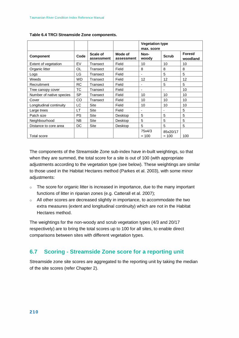
Tasmanian River Condition Index Reference Manual
210
Table 6.4 TRCI Streamside Zone components.
Vegetation type max. score
Component Code Scale of assessment
Mode of assessment
Non-woody Scrub Forest/
woodland Extent of vegetation EV Transect Field 10 10 10 Organic litter OL Transect Field 8 8 8 Logs LG Transect Field - 5 5 Weeds WD Transect Field 12 12 12 Recruitment RC Transect Field - 5 5 Tree canopy cover TC Transect Field - - 10 Number of native species SP Transect Field 10 10 10 Cover CO Transect Field 10 10 10 Longitudinal continuity LC Site Field 10 10 10 Large trees LT Site Field - - 5 Patch size PS Site Desktop 5 5 5 Neighbourhood NB Site Desktop 5 5 5 Distance to core area DC Site Desktop 5 5 5
Total score 75x4/3 = 100
85x20/17 = 100 100
The components of the Streamside Zone sub-index have in-built weightings, so that when they are summed, the total score for a site is out of 100 (with appropriate adjustments according to the vegetation type (see below). These weightings are similar to those used in the Habitat Hectares method (Parkes et al. 2003), with some minor adjustments:
o The score for organic litter is increased in importance, due to the many important functions of litter in riparian zones (e.g. Catterall et al. 2007);
o All other scores are decreased slightly in importance, to accommodate the two extra measures (extent and longitudinal continuity) which are not in the Habitat Hectares method.
The weightings for the non-woody and scrub vegetation types (4/3 and 20/17 respectively) are to bring the total scores up to 100 for all sites, to enable direct comparisons between sites with different vegetation types.
6.7 Scoring - Streamside Zone score for a reporting unit Streamside zone site scores are aggregated to the reporting unit by taking the median of the site scores (refer Chapter 2).
Tasmanian River Condition Index Reference Manual
211
6.8 Missing data Try to not have any! If a single observation is missing from one transect, the average of the values from the other transects can be substituted. Examination of the photos may also aid in recalling missing information.
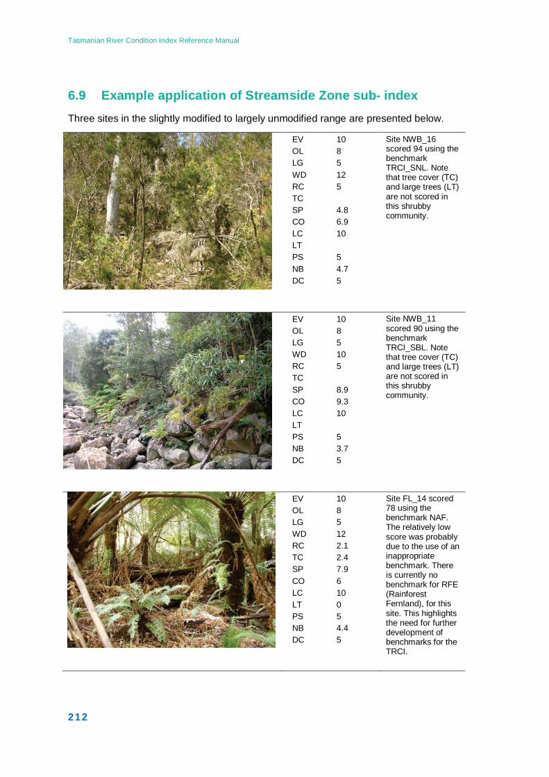
Tasmanian River Condition Index Reference Manual
212
6.9 Example application of Streamside Zone sub- index Three sites in the slightly modified to largely unmodified range are presented below.
EV 10 OL 8 LG 5 WD 12 RC 5 TC SP 4.8 CO 6.9 LC 10 LT PS 5 NB 4.7 DC 5
Site NWB_16 scored 94 using the benchmark TRCI_SNL. Note that tree cover (TC) and large trees (LT) are not scored in this shrubby community.
EV 10 OL 8 LG 5 WD 10 RC 5 TC SP 8.9 CO 9.3 LC 10 LT PS 5 NB 3.7 DC 5
Site NWB_11 scored 90 using the benchmark TRCI_SBL. Note that tree cover (TC) and large trees (LT) are not scored in this shrubby community.
EV 10 OL 8 LG 5 WD 12 RC 2.1 TC 2.4 SP 7.9 CO 6 LC 10 LT 0 PS 5 NB 4.4 DC 5
Site FL_14 scored 78 using the benchmark NAF. The relatively low score was probably due to the use of an inappropriate benchmark. There is currently no benchmark for RFE (Rainforest Fernland), for this site. This highlights the need for further development of benchmarks for the TRCI.
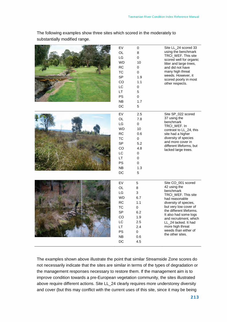
Tasmanian River Condition Index Reference Manual
213
The following examples show three sites which scored in the moderately to substantially modified range.
EV 0 OL 8 LG 0 WD 10 RC 0 TC 0 SP 1.9 CO 1.1 LC 0 LT 5 PS 0 NB 1.7 DC 5
Site LL_24 scored 33 using the benchmark TRCI_WEF. This site scored well for organic litter and large trees, and did not have many high threat weeds. However, it scored poorly in most other respects.
EV 2.5 OL 7.8 LG 0 WD 10 RC 0.6 TC 0 SP 5.2 CO 4.8 LC 0 LT 0 PS 0 NB 1.3 DC 5
Site SP_022 scored 37 using the benchmark TRCI_WEF. In contrast to LL_24, this site had a higher diversity of species and more cover in different lifeforms, but lacked large trees.
EV 5 OL 8 LG 3 WD 6.7 RC 1.1 TC 0 SP 6.2 CO 1.9 LC 2.5 LT 2.4 PS 0 NB 0.6 DC 4.5
Site CO_001 scored 42 using the benchmark TRCI_WEF. This site had reasonable diversity of species, but very low cover of the different lifeforms. It also had some logs and recruitment, which LL_24 lacked. It had more high threat weeds than either of the other sites.
The examples shown above illustrate the point that similar Streamside Zone scores do not necessarily indicate that the sites are similar in terms of the types of degradation or the management responses necessary to restore them. If the management aim is to improve condition towards a pre-European vegetation community, the sites illustrated above require different actions. Site LL_24 clearly requires more understorey diversity and cover (but this may conflict with the current uses of this site, since it may be being
Tasmanian River Condition Index Reference Manual
214
maintained as a parkland for aesthetic reasons). Site SP_022 may only require protection from further disturbance to improve condition, since there appears to be a reasonable diversity of species already present, and only time will provide large trees. Examination of the field data would reveal whether particular lifeforms are missing from the species complement and would need to be planted to improve condition. Site CO_001 clearly requires management of the high threat weeds present, and examination of the field data collected would enable a strategy to be developed to achieve this.
6.10 References - Streamside Zone Askey-Doran, M. (1993) Riparian vegetation in the Midlands and Eastern Tasmania. Department of Environment and Land Management – Parks and Wildlife Service, Hobart Tasmania.
Catterall, C.P., Lynch, R.J. & Jansen, A. (2007) Riparian wildlife and habitats. In Principles for riparian lands management (eds S. Lovett & P. Price), pp. 141-58. Land and Water Australia, Canberra.
DSE (2006). Index of Stream Condition User’s Manual (2nd edition). Victorian Government Department of Sustainability and Environment, Melbourne.
Harris, S and Kitchener, A (2005) From Forest to Fjeldmark: Descriptions of Tasmania’s Vegetation. Department of Primary Industries ,Water and Environment, Printing Authority of Tasmania. Hobart.
Jansen, A, Robertson, A, Thompson, L & Wilson, A. (2005) Development and application of a method for the rapid appraisal of riparian condition. River and Riparian Land Management Technical Guideline, No. 4A. Canberra: Land & Water Australia. http://www.rivers.gov.au/publicat/guidemanual.htm
Michaels, K. (2006), A Manual for Assessing Vegetation Condition in Tasmania, Version 1.0. Resource Management and Conservation, Department of Primary Industries, Water and Environment, Hobart.
Parkes, D., Newell, G., Cheal, D. (2003). Assessing the quality of native vegetation: The ‘habitat hectares’ approach. Journal of Ecological Management & Restoration 4 supplement, S29-S38.
Slijkerman, J., Kaye, J., Jansen A and Brown, M. (2007) Tasmanian River Condition Index: Testing the Draft Method, Pilot Results and Analysis- Streamside Zone Sub-Index. A report to NRM South. Earth Tech. Wangaratta, Victoria.
Tolsma, A. & Newell, G. (2003). Assessing the quality of native vegetation: further development of the ‘Habitat Hectares’ approach. State of Victoria, Department of Sustainability and Environment.

Tasmanian River Condition Index Reference Manual
215
White, L.J., and Ladson, A.R., (1999) ‘An Index of Stream Condition: Reference Manual (second edition), Department of Natural Resources and Environment, Melbourne

Tasmanian River Condition Index Reference Manual
216
Appendix to Chapter 6: Further detail on the Streamside Zone sub-index Appendix 6.1 The development of Streamside Zone (riparian) benchmarks
Appendix 6.2 TRCI riparian vegetation communities - benchmark values table, description and key
Appendix 6.3 Data sheets, high threat weed list and TRCI lifeform definitions.
Appendix 6.4 Scoring
Tasmanian River Condition Index Reference Manual
217
Appendix 6.1 The development of Streamside Zone (riparian) vegetation benchmarks
Background Vegetation condition benchmarks (TASVEG) have been developed for the majority of vegetation communities in Tasmania (Michaels 2006). Some of these benchmarks are specifically for various riparian vegetation types and are potentially directly applicable to the TRCI. In many cases, however, riparian vegetation types do not fit any of the existing benchmarks, or the existing benchmarks are not appropriate. In addition, due to some differences in the methods and types of data collected, TASVEG benchmarks need to be adapted for use in the TRCI.
Options for producing vegetation benchmarks suitable for the TRCI included:
o adopting the TASVEG benchmarks which were applicable to riparian vegetation, with adjustments for the TRCI method, adapting existing benchmarks to suit riparian conditions, and developing new ones to suit all of the remaining riparian vegetation types not covered by existing benchmarks
o developing an independent set of ‘riparian’ vegetation benchmarks synthetically, as was done for TASVEG
o developing riparian benchmarks from existing floristic and structural data on riparian vegetation
o developing ‘generic’ benchmarks to suit a range of riparian vegetation types, either synthetically or with reference to existing data.
Process Working group meetings were convened to examine the existing TASVEG benchmarks for suitability, and sources of potential data on riparian vegetation were determined. The working group consisted of Dr Mick Brown, Dr Amy Jansen, Johanna Slijkerman, Michael Askey-Doran and Jamie Kaye. A list of existing TASVEG benchmarks which were deemed suitable ‘as is’ (apart from adjustment to suit the TRCI method) was derived from Michaels (2006) and Harris & Kitchener (2005). Expert panel discussions determined that the majority of the remaining riparian vegetation types in Tasmania could be classified into the following groups:
o Wet eucalypt forests with rainforest, broad-leaved shrub or Leptospermum-dominated understoreys;
o Dry eucalypt forests and woodlands with narrow-leaved or broad-leaved shrub understoreys;
o Grasslands.
Floristic data from Askey-Doran (1993) were used to confirm these riparian communities, and to derive benchmark values for these generic communities for TRCI
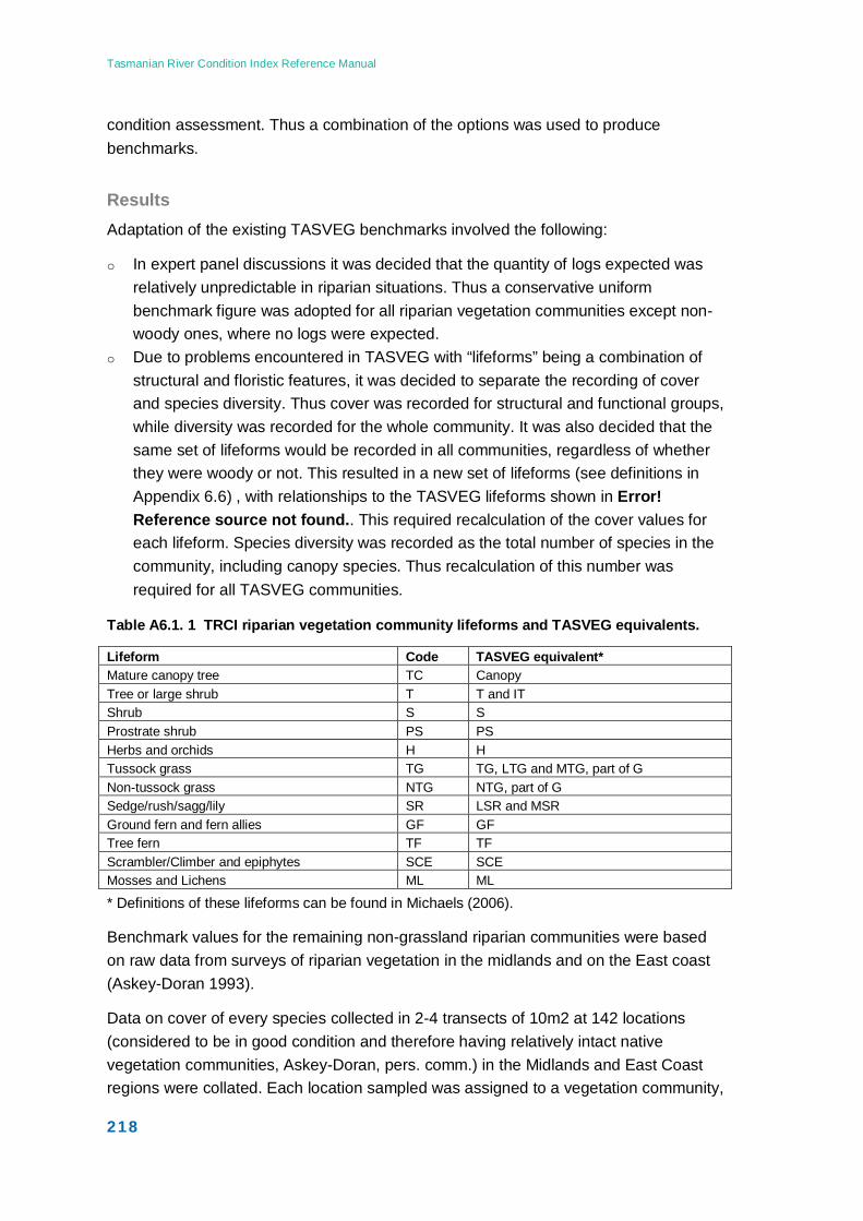
Tasmanian River Condition Index Reference Manual
218
condition assessment. Thus a combination of the options was used to produce benchmarks.
Results Adaptation of the existing TASVEG benchmarks involved the following:
o In expert panel discussions it was decided that the quantity of logs expected was relatively unpredictable in riparian situations. Thus a conservative uniform benchmark figure was adopted for all riparian vegetation communities except non-woody ones, where no logs were expected.
o Due to problems encountered in TASVEG with “lifeforms” being a combination of structural and floristic features, it was decided to separate the recording of cover and species diversity. Thus cover was recorded for structural and functional groups, while diversity was recorded for the whole community. It was also decided that the same set of lifeforms would be recorded in all communities, regardless of whether they were woody or not. This resulted in a new set of lifeforms (see definitions in Appendix 6.6) , with relationships to the TASVEG lifeforms shown in Error! Reference source not found.. This required recalculation of the cover values for each lifeform. Species diversity was recorded as the total number of species in the community, including canopy species. Thus recalculation of this number was required for all TASVEG communities.
Table A6.1. 1 TRCI riparian vegetation community lifeforms and TASVEG equivalents.
Lifeform Code TASVEG equivalent* Mature canopy tree TC Canopy Tree or large shrub T T and IT Shrub S S Prostrate shrub PS PS Herbs and orchids H H Tussock grass TG TG, LTG and MTG, part of G Non-tussock grass NTG NTG, part of G Sedge/rush/sagg/lily SR LSR and MSR Ground fern and fern allies GF GF Tree fern TF TF Scrambler/Climber and epiphytes SCE SCE Mosses and Lichens ML ML
* Definitions of these lifeforms can be found in Michaels (2006).
Benchmark values for the remaining non-grassland riparian communities were based on raw data from surveys of riparian vegetation in the midlands and on the East coast (Askey-Doran 1993).
Data on cover of every species collected in 2-4 transects of 10m2 at 142 locations (considered to be in good condition and therefore having relatively intact native vegetation communities, Askey-Doran, pers. comm.) in the Midlands and East Coast regions were collated. Each location sampled was assigned to a vegetation community,
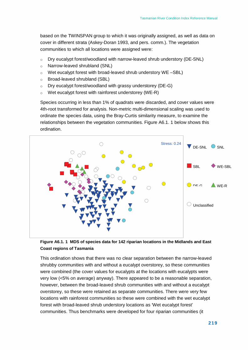
Tasmanian River Condition Index Reference Manual
219
based on the TWINSPAN group to which it was originally assigned, as well as data on cover in different strata (Askey-Doran 1993, and pers. comm.). The vegetation communities to which all locations were assigned were:
o Dry eucalypt forest/woodland with narrow-leaved shrub understory (DE-SNL) o Narrow-leaved shrubland (SNL) o Wet eucalypt forest with broad-leaved shrub understory WE –SBL) o Broad-leaved shrubland (SBL) o Dry eucalypt forest/woodland with grassy understorey (DE-G) o Wet eucalypt forest with rainforest understorey (WE-R)
Species occurring in less than 1% of quadrats were discarded, and cover values were 4th-root transformed for analysis. Non-metric multi-dimensional scaling was used to ordinate the species data, using the Bray-Curtis similarity measure, to examine the relationships between the vegetation communities. Figure A6.1. 1 below shows this ordination.
Figure A6.1. 1 MDS of species data for 142 riparian locations in the Midlands and East Coast regions of Tasmania
This ordination shows that there was no clear separation between the narrow-leaved shrubby communities with and without a eucalypt overstorey, so these communities were combined (the cover values for eucalypts at the locations with eucalypts were very low (<5% on average) anyway). There appeared to be a reasonable separation, however, between the broad-leaved shrub communities with and without a eucalypt overstorey, so these were retained as separate communities. There were very few locations with rainforest communities so these were combined with the wet eucalypt forest with broad-leaved shrub understory locations as ‘Wet eucalypt forest’ communities. Thus benchmarks were developed for four riparian communities (it
Stress: 0.24 DE-SNL SNL
SBL WE-SBL
DE-G WE-R
Unclassified
Tasmanian River Condition Index Reference Manual
220
should be noted that as there were few locations assigned to the ‘Wet eucalypt forest’ community, the benchmark developed may need revision once additional data becomes available).
To develop the benchmarks, species were assigned to lifeforms (Askey-Doran, pers. comm.), and mean data on lifeform cover, species diversity and litter cover were calculated from data for each location, according to the vegetation community to which they had been assigned.
A synthetic benchmark was created for riparian grassland communities, by averaging TASVEG benchmark values for four grassland communities considered to occur in riparian situations (GPH, GCL, GPL, GTL).
The riparian vegetation communities identified in this process are described in Appendix 6.2. Note that the TRCI communities derived from Askey-Doran (1993) are described based on the benchmark data for these communities. For the communities adopted from TASVEG the descriptions are as they appear for TASVEG - these may need to be revised once there is more data available for riparian communities. The communities without benchmarks are as described by Harris & Kitchener (2005).

Tasmanian River Condition Index Reference Manual
221

Tasmanian River Condition Index Reference Manual
222
Appendix 6.2 TRCI riparian vegetation communities The benchmark values for TRCI riparian vegetation communities are presented in Table A6.2. 1. This is followed by a description of each community and a key for determining the most appropriate pre 1750 community in the field.
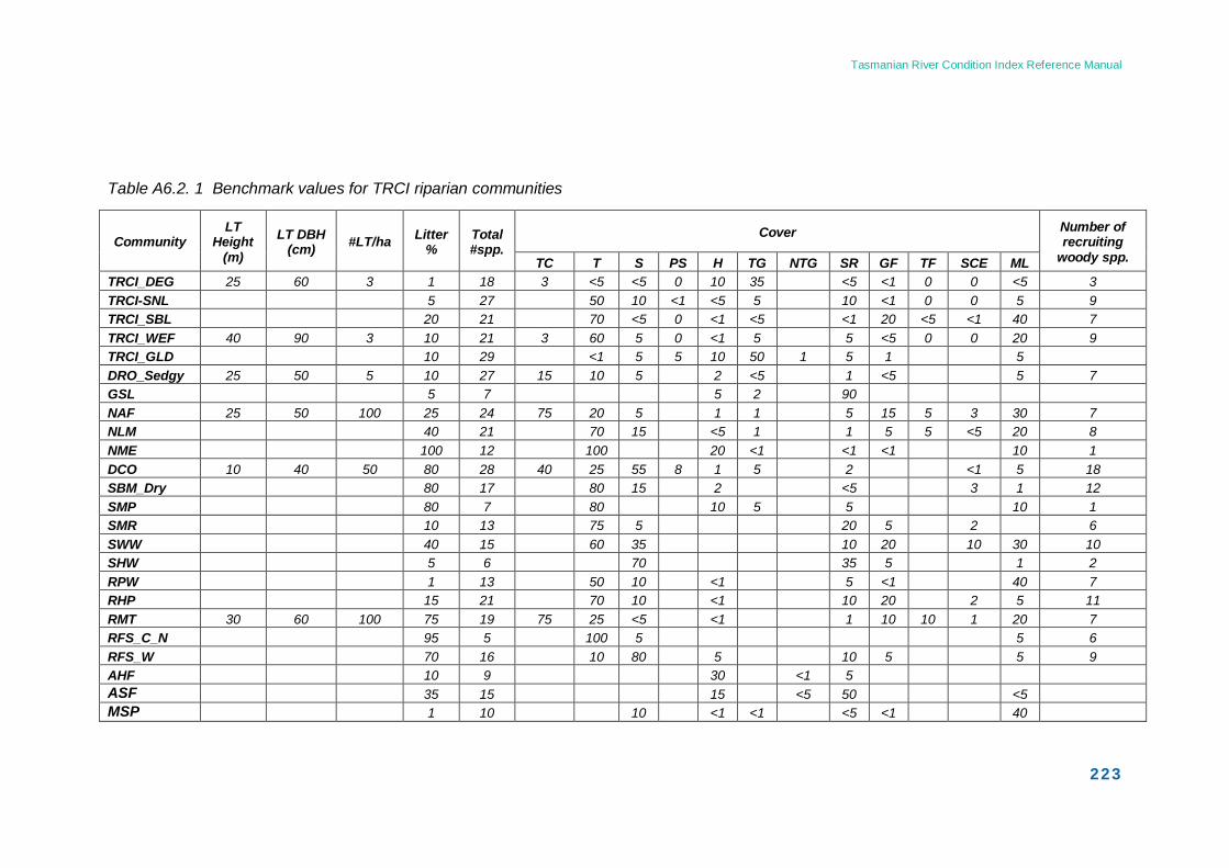
Tasmanian River Condition Index Reference Manual
223
Table A6.2. 1 Benchmark values for TRCI riparian communities
Community LT
Height (m)
LT DBH (cm) #LT/ha Litter
% Total #spp.
Cover Number of recruiting
woody spp. TC T S PS H TG NTG SR GF TF SCE ML TRCI_DEG 25 60 3 1 18 3 <5 <5 0 10 35 <5 <1 0 0 <5 3 TRCI-SNL 5 27 50 10 <1 <5 5 10 <1 0 0 5 9 TRCI_SBL 20 21 70 <5 0 <1 <5 <1 20 <5 <1 40 7 TRCI_WEF 40 90 3 10 21 3 60 5 0 <1 5 5 <5 0 0 20 9 TRCI_GLD 10 29 <1 5 5 10 50 1 5 1 5 DRO_Sedgy 25 50 5 10 27 15 10 5 2 <5 1 <5 5 7 GSL 5 7 5 2 90 NAF 25 50 100 25 24 75 20 5 1 1 5 15 5 3 30 7 NLM 40 21 70 15 <5 1 1 5 5 <5 20 8 NME 100 12 100 20 <1 <1 <1 10 1 DCO 10 40 50 80 28 40 25 55 8 1 5 2 <1 5 18 SBM_Dry 80 17 80 15 2 <5 3 1 12 SMP 80 7 80 10 5 5 10 1 SMR 10 13 75 5 20 5 2 6 SWW 40 15 60 35 10 20 10 30 10 SHW 5 6 70 35 5 1 2 RPW 1 13 50 10 <1 5 <1 40 7 RHP 15 21 70 10 <1 10 20 2 5 11 RMT 30 60 100 75 19 75 25 <5 <1 1 10 10 1 20 7 RFS_C_N 95 5 100 5 5 6 RFS_W 70 16 10 80 5 10 5 5 9 AHF 10 9 30 <1 5 ASF 35 15 15 <5 50 <5 MSP 1 10 10 <1 <1 <5 <1 40

Tasmanian River Condition Index Reference Manual
224
Descriptions of riparian vegetation communities in Tasmania *Note: benchmark values are not currently available for communities marked with an asterisk (RMS, RKP and RFE).
Dry Eucalypt forest and woodland with grassy understorey TRCI_DEG: Most or all trees in tallest stratum belong to the genus Eucalyptus with at least 5% solid canopy cover, understorey predominantly a grassy ground layer.
Narrow-leaved shrubby scrub TRCI_SNL: Most or all trees in tallest stratum belong to the genus Eucalyptus, if present; understorey predominantly hard-leaved (sclerophyllous) shrubs.
Broad-leaved shrubby scrub TRCI_SBL: Scrub dominated by broad-leaf shrubs such as Beyeria viscosa, Bedfordia salicina, Pomaderris apetala, Notelaea or Leptospermum lanigerum over Bauera rubioides and rainforest species seedlings.
Wet Eucalypt forest TRCI_WEF: Most or all trees in tallest stratum belong to the genus Eucalyptus with at least 5% solid canopy cover, understorey includes any of the following: a) Nothofagus, Atherosperma, Athrotaxis, Eucryphia, Phyllocladus or Lagarostrobos prominent as secondary trees or shrubs; b) a tree or tall shrub layer dominated either by species with leaves more than 1cm wide or species of Leptospermum or Melaleuca, c) a layer dominated by ferns other than bracken.
Grassland TRCI_GLD: Vegetation dominated by native grasses (with cover > 25% native species).
Eucalyptus rodwayii forest and woodland, sedgy variant DRO sedgy: Eucalyptus rodwayi forest and woodland are communities dominated by E. rodwayi on fertile valley flats, usually subject to water logging. The understorey is sedgy. The degree of site exposure and severity of frosts and waterlogging influence the form of the community. Towards the centre of marshes, mallee-form trees (< 10m) occur as a sporadic component of low, open woodland and sedgeland/ heathland. Low, open woodland structure is also found on exposed sites subject to severe frosts. Woodlands and open forests (> 40m) are found in more sheltered situations and on better aerated sites around the perimeter of marshes and flats.
Lowland grassy sedgeland GSL: Lowland grassy sedgeland is dominated by sedges such as Lomandra longifolia and Lepidosperma species interspersed with grasses.
Acacia melanoxylon swamp forest NAF: Acacia melanoxylon swamp forest is typically a tall closed forest (> 30m in height) dominated by Acacia melanoxylon with a relatively open and variable understorey. Nothofagus cunninghamii and other rainforest species are present at some sites that have not had major disturbance for a long period. On more recently disturbed sites, Melaleuca squarrosa, M. ericifolia and one or more species of Leptospermum may be present. Hummocks of Sphagnum species associated with myrtle logs occur in successionally advanced forest.
Tasmanian River Condition Index Reference Manual
225
Leptospermum lanigerum – Melaleuca squarrosa swamp forest NLM: Leptospermum lanigerum – Melaleuca squarrosa swamp forests dominated by Leptospermum lanigerum and/or Melaleuca squarrosa are common in the north-west and west and occur occasionally in the north-east and east where L. lanigerum usually predominates. There are also extensive tracts on alluvial flats of the major south-west rivers. The forests are dominated by various mixtures of L. lanigerum and M. squarrosa but with varying lesser amounts of various species of Acacia and rainforest species also present. Trees are usually > 8m in height.
Melaleuca ericifolia swamp forest NME: Melaleuca ericifolia swamp forest typically occurs as pure or almost pure stands of Melaleuca ericifolia with trees generally 10 – 12m in height (but reaching 20m) forming a dense canopy. The understorey is generally simple and devoid of shrubs due to low light levels and/or frequent flooding. It is most often dominated by Carex appressa and/or Gahnia grandis and Blechnum wattsii and Lepidosperma elatius may be present.
Eucalyptus coccifera forest and woodland DCO: Eucalyptus coccifera forest and woodland is a forest woodland complex that is widespread in the subalpine areas of Tasmania over about 600m above sea level. The type is primarily but not always associated with dolerite substrates. E. coccifera forests up to 20m in height are generally restricted to sheltered sites. Woodland trees generally vary from 5 – 10m in height. The understorey generally has a significant heathy or shrubby component.
Banksia marginata wet scrub SBM: Banksia marginata wet scrub is a dense wet scrub dominated by Banksia marginata occurring in two recognised facies. SBM dry facies is found on creek fringes within south-west buttongrass moorland and is rich in Melaleuca squarrosa, Leptospermum scoparium and sometimes L. nitidum, often with Gahnia grandis and Empodisma minus or Calorophus species tangled through. SBM wet facies is not a riparian vegetation community.
Melaleuca pustulata scrub SMP: Melaleuca pustulata scrub is a tall to medium dense shrubby vegetation dominated by Melaleuca pustulata occurring along creeks and hill slopes on a range of soil types over dolerite. This community is confined to the central east coast from around Swansea to Cherry Tree Hill and inland to the lower slopes of the Eastern Tiers.
Melaleuca squarrosa scrub SMR: Melaleuca squarrosa scrub is a closed canopy scrub 2-3 (5)m high on poorly drained flats underlain by peat developed on various substrates. Melaleuca squarrosa dominates, usually with some of M. squamea, Banksia marginata, Hakea epiglottis and Acacia mucronata. There may be openings of buttongrass or sedges such as Baloskion tetraphyllum, Leptocarpus tenax, Lepyrodia tasmanica and Gahnia grandis. Melaleuca squarrosa scrub is widespread through western Tasmania, especially in lowland areas of poor drainage surrounded by heathland and sedgeland. The community also occurs in the north-east and far north-west of Tasmania.
Tasmanian River Condition Index Reference Manual
226
Western wet scrub SWW: Western wet scrub is a dense, uneven scrub with up to five teatree and paperbark species plus Acacia mucronata and Bauera rubioides, often with Banksia marginata and Monotoca submutica. Eucalyptus nitida saplings are emergent. Western wet scrub is abundant in western Tasmania from near sea level to about 750m.
Wet heathland SHW: Wet heathland is a scrub community to 2m tall, commonly with scattered emergent Eucalyptus rodwayi or E. ovata and a dense ground cover of Restionaceae and Cyperaceae species. Typical dominants are Melaleuca squamea, Melaleuca gibbosa, Callistemon viridiflorus, Leptospermum species and sometimes Hakea species. The ferns Selaginella uliginosa and Lindsaea linearis are almost always present in the ground. This community generally occurs on poorly-drained head-water flats at mid-altitudes.
Athrotaxis cupressoides open woodland RPW: Athrotaxis cupressoides open woodland is vegetation (generally above 900m) in which Athrotaxis cupressoides (5 – 8m) forms small woodland patches or appears as copses and small trees scattered through alpine heathland, sedgeland, fernland and Sphagnum bogs, and along creeklines and lake margins protected from fire. On the Central Plateau and Mount Field broad poorly drained valleys and small glacial depressions may be occupied by Sphagnum cristatum bogs with emergent Athrotaxis cupressoides.
Lagarostrobos franklinii rainforest and scrub RHP: Lagarostrobos franklinii rainforest and scrub is dominated by or has a significant component of Lagarostrobos franklinii usually combined with rainforest species and sometimes Acacia melanoxylon in the canopy over an understorey of other rainforest species. Sometimes L. franklinii forms pure stands with sparse, shrubby or implicate understoreys, usually on deep alluvium. Rocky streamside short forest and scrub may have a combination of small trees of L. franklinii, Leptospermum species, Proteaceae species, rainforest and riverine species and be quite diverse. Trees can reach heights of up to 30m.
Nothofagus – Atherosperma rainforest RMT: Nothofagus – Atherosperma rainforest is tall (25+m) rainforest in which the canopy is dominated by Nothofagus cunninghamii, and sometimes Atherosperma moschatum on relatively fertile soils. Eucryphia lucida may co-dominate. Structure varies from callidendrous to thamnic, where in the latter, there are Trochocarpa species and/ or Anopterus glandulosus and other broadleaf shrubs in the understorey.
Nothofagus gunnii rainforest and scrub RFS: Nothofagus gunnii rainforest and scrub may be dense and continuous or form mosaics with alpine heathlands and sedgeland. In the central highlands and Cradle Mountain - Lake St. Clair National Park there may be few other species apart from sparsely scattered emergent Athrotaxis cupressoides and/or A. selaginoides (RFS central and northern). In the west, this community generally has an uneven canopy and is floristically diverse (RFS western). Subalpine N. gunnii / Diselma archeri scrubs occur on parts of the Mount Read
Tasmanian River Condition Index Reference Manual
227
Plateau, while a subalpine facies north-east of Mt. Bobs lacks D. archeri but has “stumps” of Dracophyllum milliganii.
Freshwater aquatic herbland AHF: Freshwater aquatic herbland is characterised by the presence of standing permanent or semi-permanent freshwater that supports aquatic and/or emergent herbaceous vegetation. It can be found from coastal to alpine elevations. This community can occur in water from a few centimetres to several metres in depth but is usually at its most diverse in shallow water less than 1m deep. Areas with clear water support the most species diverse communities while silty and tannin stained water support sparser and less diverse communities. Note, this benchmark has been determined assuming the wetland is ‘wet’.
Freshwater aquatic sedgeland and rushland ASF: Freshwater aquatic sedgeland and rushland includes wetlands dominated by sedges and rushes, with salinity ranging from fresh to brackish that occupy a diverse array of habitats from coastal to subalpine areas. A dense to sparse sward of a sedge or rush species (usually one species dominates) provides the tallest stratum in a sedge/rush wetland. A variety of smaller sedges and herbs commonly form a sparse to dense layer between and below this. The dominant sedges and rushes are generally greater than 50cm in height.
Sphagnum peatland MSP: Treeless Sphagnum communities cover a range of different Sphagnum peatland types, including tussock grassland mires, buttongrass Sphagnum bogs and floating aquatic Sphagnum mires. The most common type is the shrub-dominated Richea-Sphagnum bogs. They range in size from small patches to > 5ha in size. The moss-derived peats range from quite shallow to 2m deep. Sphagnum peatlands can be almost pure moss beds, dominant or co-dominant with the sedges Empodisma minus, Baloskion australe, Gahnia grandis and Gymnoschoenus sphaerocephalus, with Gleichenia alpina and/or the shrubs Richea scoparia, Richea gunnii, Baeckea gunniana, Epacris serpyllifolia and/or Callistemon spp.
Nothofagus–Phyllocladus short rainforest RMS*: Nothofagus–Phyllocladus short rainforest is typically short (8–20m), often implicate rainforest vegetation with moderate to high floristic diversity. It has several co-dominant canopy species including Nothofagus cunninghamii, Phyllocladus aspleniifolius and Eucryphia lucida. Eucalyptus nitida is an occasional emergent. It occupies low to moderately fertile sites in western Tasmania.
Athrotaxis selaginoides rainforest RKP*: This community can form pure stands of Athrotaxis selaginoides, but more commonly the conifer is co-dominant with or subdominant to Nothofagus cunninghamii in medium forests. The short forests may be floristically simple but often are highly diverse, at low altitudes (from about 250m to 500m) near the West Coast Range.
Rainforest Fernland RFE*: This community consists of dense Dicksonia antarctica cover occupying broad gullies, where trees are locally absent, amidst rainforest.
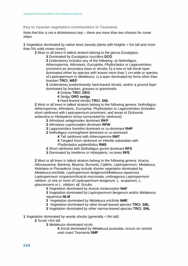
Tasmanian River Condition Index Reference Manual
228
Key to riparian vegetation communities in Tasmania Note that this is not a dichotomous key – there are more than two choices for some steps. 1 Vegetation dominated by native trees (woody plants with heights > 5m tall and more than 5% solid crown cover).
2 Most or all trees in tallest stratum belong to the genus Eucalyptus 3 Dominated by Eucalyptus coccifera DCO 3 Understorey includes any of the following: a) Nothofagus, Atherosperma, Athrotaxis, Eucryphia, Phyllocladus or Lagarostrobos prominent as secondary trees or shrubs; b) a tree or tall shrub layer dominated either by species with leaves more than 1 cm wide or species of Leptospermum or Melaleuca, c) a layer dominated by ferns other than bracken TRCI_WEF 3 Understorey predominantly hard-leaved shrubs, and/or a ground layer dominated by bracken, grasses or graminoids
4 Grassy TRCI_DEG 4 Sedgy DRO sedgy
4 Hard-leaved shrubs TRCI_SNL 2 Most or all trees in tallest stratum belong to the following genera: Nothofagus, Atherosperma, Athrotaxis, Eucryphia, Phyllocladus or Lagarostrobos (includes short rainforest with Leptospermum prominent, and areas of Dicksonia antarctica or Histiopteris incisa surrounded by rainforest)
3 Athrotaxis selaginoides dominant RKP 3 Athrotaxis cupressoides dominant RPW 3 Lagarostrobos franklinii dominant or co-dominant RHP 3 Nothofagus cunninghamii dominant or co-dominant
4 Tall rainforest with Atherosperma RMT 4 Tangled short rainforest on infertile substrates with Phyllocladus aspleniifolius RMS
3 Short rainforest with Nothofagus gunnii dominant RFS 3 Dominated by treeferns or Histiopteris, no trees RFE
2 Most or all trees in tallest stratum belong to the following genera: Acacia, Allocasuarina, Banksia, Beyeria, Bursaria, Callitris, Leptospermum, Melaleuca, Notelaea or Pomaderris (may include shorter vegetation dominated by Melaleuca ericifolia, Leptospermum lanigerum/Melaleuca squarrosa, Leptospermum scoparium/Acacia mucronata, umbrageous Leptospermum nitidum, or one or more of Leptospermum lanigerum, L. scoparium, L. glaucescens or L. nitidum; cf. Scrubs
3 Vegetation dominated by Acacia melanoxylon NAF 3 Vegetation dominated by Leptospermum lanigerum and/or Melaleuca squarrosa NLM 3 Vegetation dominated by Melaleuca ericifolia NME 3 Vegetation dominated by other broad-leaved species TRCI_SBL 3 Vegetation dominated by other narrow-leaved species TRCI_SNL
1 Vegetation dominated by woody shrubs (generally < 8m tall)
2 Scrub >2m tall 3 Melaleuca–dominated scrub
4 Scrub dominated by Melaleuca pustulata, occurs on central east coast Tasmania SMP
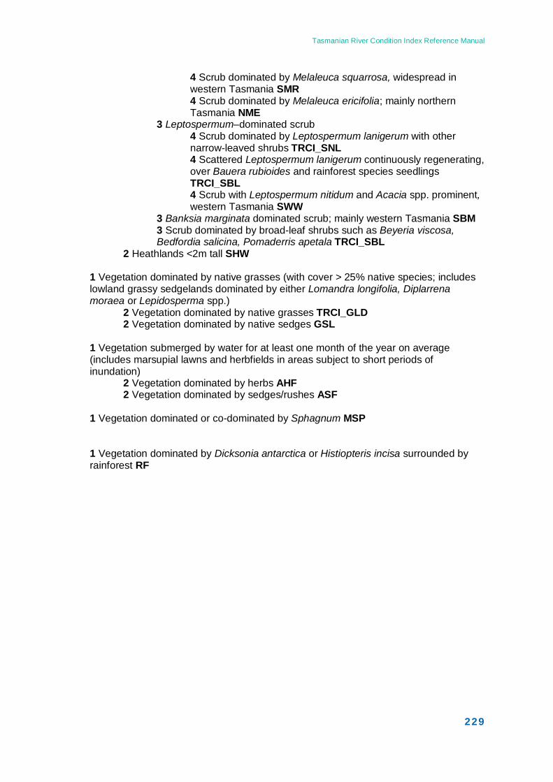
Tasmanian River Condition Index Reference Manual
229
4 Scrub dominated by Melaleuca squarrosa, widespread in western Tasmania SMR 4 Scrub dominated by Melaleuca ericifolia; mainly northern Tasmania NME
3 Leptospermum–dominated scrub 4 Scrub dominated by Leptospermum lanigerum with other narrow-leaved shrubs TRCI_SNL 4 Scattered Leptospermum lanigerum continuously regenerating, over Bauera rubioides and rainforest species seedlings TRCI_SBL 4 Scrub with Leptospermum nitidum and Acacia spp. prominent, western Tasmania SWW
3 Banksia marginata dominated scrub; mainly western Tasmania SBM 3 Scrub dominated by broad-leaf shrubs such as Beyeria viscosa, Bedfordia salicina, Pomaderris apetala TRCI_SBL
2 Heathlands <2m tall SHW 1 Vegetation dominated by native grasses (with cover > 25% native species; includes lowland grassy sedgelands dominated by either Lomandra longifolia, Diplarrena moraea or Lepidosperma spp.) 2 Vegetation dominated by native grasses TRCI_GLD
2 Vegetation dominated by native sedges GSL 1 Vegetation submerged by water for at least one month of the year on average (includes marsupial lawns and herbfields in areas subject to short periods of inundation) 2 Vegetation dominated by herbs AHF 2 Vegetation dominated by sedges/rushes ASF 1 Vegetation dominated or co-dominated by Sphagnum MSP 1 Vegetation dominated by Dicksonia antarctica or Histiopteris incisa surrounded by rainforest RF

Tasmanian River Condition Index Reference Manual
230
6.10.1 Appendix 6.3 Data sheets These data sheets are also available as a separate file from NRM South.

Tasmanian River Condition Index Reference Manual
231
TRCI Streamside Zone Site Details Date:
Site ID: Waterway:GPS (Datum UTM GDA94)
NRM Region: Start easting:
Reporting Unit: Start northing:
Assessors: End easting:
End northing:
Bank (circle): left / right GPS accuracy: m(determined facing downstream)
Site direction (circle): upstream / downstream
Bankfull channel width at start: m
Total site length (15 x bankfull channel width, min. 90m max. 450m): m
Access details, property name:
Start of siteTransect 1Transect 2Transect 3Transect 4End of siteOther:
Vegetation community
Vegetation type (circle):
Landscape components (desktop assessed)Patch size Neighbourhood
Distance to Core Area
Area (ha)
Distance (km)
Radius from Site100m1km5km
% Native Vegetation
Photographs (record photo numbers from review screen on camera)Along bank Away from channel Towards channel
Please note any other clues which may assist in identifying the riparian community, particularly if it is very altered e.g. nearby vegetation (upslope, across the stream)
TasVeg code and description (from map):
Most likely TRCI benchmark:
–canopy tree species with dbh>50cm (except for E. coccifera where dbh>40cm) and solid crown cover >5% –woody species with dbh<50cm or solid crown cover of canopy trees <5% –lack significant woody species (<5% cover of trees and/or shrubs).
ScrubNon-woody
Forest/woodland
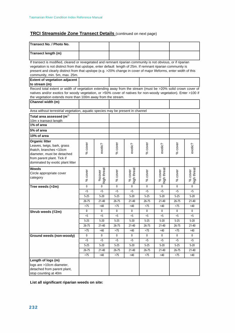
Tasmanian River Condition Index Reference Manual
232
TRCI Streamside Zone Transect Details (continued on next page)
Transect No. / Photo No.
Transect length (m)
Extent of vegetation adjacent to stream (m)
Channel width (m)
Total area assessed (m2)
10m x transect length1% of area5% of area10% of area
% c
over
exot
ic?
% c
over
exot
ic?
% c
over
exot
ic?
% c
over
exot
ic?
WeedsCircle appropriate cover category
% c
over
%co
ver
high
thre
at
% c
over
% c
over
hi
gh th
reat
% c
over
% c
over
hi
gh th
reat
% c
over
% c
over
hi
gh th
reat
0 0 0 0 0 0 0 0<5 <5 <5 <5 <5 <5 <5 <5
5-25 5-20 5-25 5-20 5-25 5-20 5-25 5-2026-75 21-40 26-75 21-40 26-75 21-40 26-75 21-40>75 >40 >75 >40 >75 >40 >75 >400 0 0 0 0 0 0 0<5 <5 <5 <5 <5 <5 <5 <5
5-25 5-20 5-25 5-20 5-25 5-20 5-25 5-2026-75 21-40 26-75 21-40 26-75 21-40 26-75 21-40>75 >40 >75 >40 >75 >40 >75 >400 0 0 0 0 0 0 0<5 <5 <5 <5 <5 <5 <5 <5
5-25 5-20 5-25 5-20 5-25 5-20 5-25 5-2026-75 21-40 26-75 21-40 26-75 21-40 26-75 21-40>75 >40 >75 >40 >75 >40 >75 >40
Length of logs (m)logs are >10cm diameter, detached from parent plant, stop counting at 40m
List all significant riparian weeds on site:
Area without terrestrial vegetation, aquatic species may be present in channel
Record total extent or width of vegetation extending away from the stream (must be >20% solid crown cover ofnatives and/or exotics for woody vegetation, or >50% cover of natives for non-woody vegetation). Enter >100 ifthe vegetation extends more than 100m away from the stream.
If transect is modified, cleared or revegetated and remnant riparian community is not obvious, or if riparian vegetation is not distinct from that upslope, enter default length of 25m. If remnant riparian community is present and clearly distinct from that upslope (e.g. >20% change in cover of major lifeforms, enter width of this community, min. 5m, max. 25m.
Ground weeds (non-woody)
Shrub weeds (≤2m)
Tree weeds (>2m)
Organic litterLeaves, twigs, bark, grass thatch, branches <10cm diameter, must be detached from parent plant. Tick if dominated by exotic plant litter
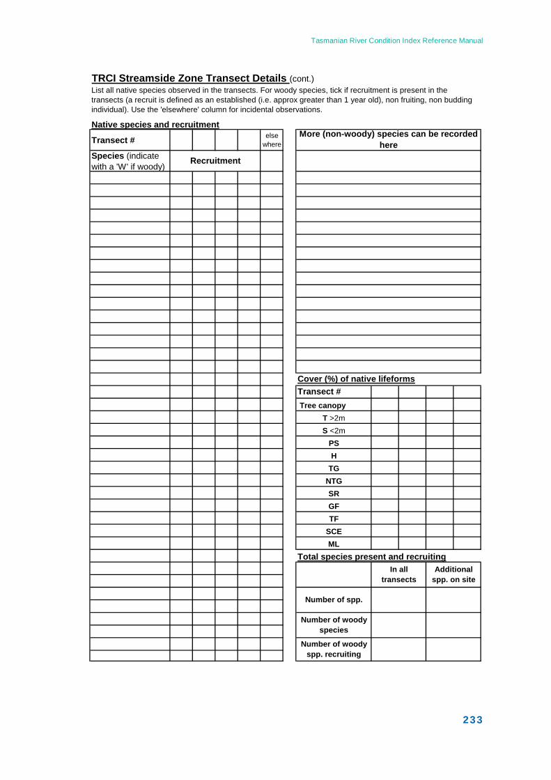
Tasmanian River Condition Index Reference Manual
233
TRCI Streamside Zone Transect Details (cont.)
Transect # else where
Species (indicate with a 'W' if woody)
Transect # Tree canopy
T >2mS <2m
PSH
TGNTGSRGFTF
SCEML
Total species present and recruiting
Native species and recruitment
Recruitment
List all native species observed in the transects. For woody species, tick if recruitment is present in the transects (a recruit is defined as an established (i.e. approx greater than 1 year old), non fruiting, non budding individual). Use the 'elsewhere' column for incidental observations.
Number of spp.
Additional spp. on site
More (non-woody) species can be recorded here
Cover (%) of native lifeforms
In all transects
Number of woody species
Number of woody spp. recruiting

Tasmanian River Condition Index Reference Manual
234
TRCI Streamside Zone: Whole of Site
Continuous native (woody or non-woody) dominant
Continuous exotic woody dominant*
Break
Count
Total
Site observations (circle answers)
Comments?
Can livestock access the site? yes / no / partial / unsure Total: Total: Total:Total number of breaks: TypeTotal length of site:* Add 'W' if willows dominate.
Site diagram, notes, comments:
Longitudinal Continuity Record zero (at end of site) and meterage at each change. Continuous: woody vegetation (>20% solid cover native or exotic) or native non-woody vegetation (>50% cover), >10m long, >5m wide from toe of bank. Break: vegetation not as above, and >10m long. Alive
Recent fencing/reveg/improvement works (specify details, timing)
Recent disturbance events? i.e. Flood, fire, other, specify details (note if the vegetation community is a successional type due to this disturbance)
Grazing pressure? High / medium / low
Large Trees For E. coccifera forest/woodland, large trees are >40cm dbh; For A. melanoxylon forest and E rodwayi forest/woodland large trees are >50cm dbh; For wet Eucalypt forests, large trees are >90cm dbh; oherwise large trees are >60cm dbh (circle which dbh was used).
Is the vegetation community on site in relatively ‘good condition’? i.e. suitable to use as a reference: yes / no
If the site is surrounded by grassland, is it dominated by native or exotic species? native / exotic
Average transect width (m):Site area (m2):
Dead
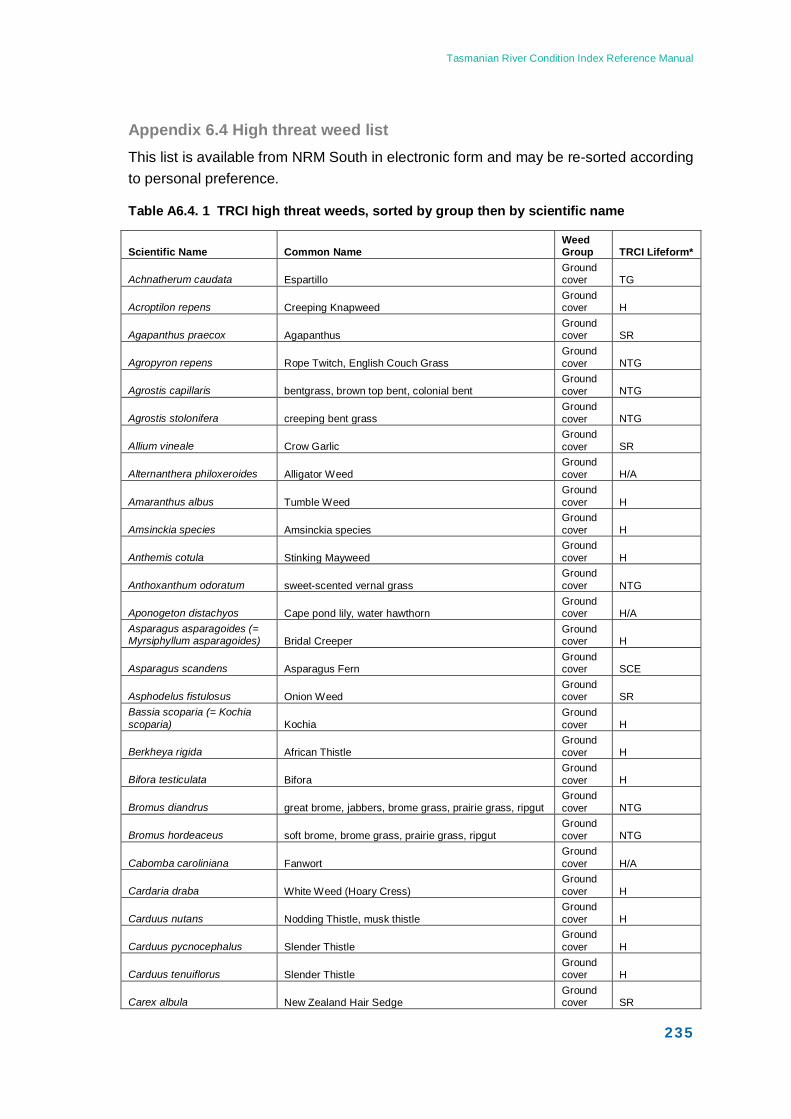
Tasmanian River Condition Index Reference Manual
235
Appendix 6.4 High threat weed list This list is available from NRM South in electronic form and may be re-sorted according to personal preference.
Table A6.4. 1 TRCI high threat weeds, sorted by group then by scientific name
Scientific Name Common Name Weed Group TRCI Lifeform*
Achnatherum caudata Espartillo Ground cover TG
Acroptilon repens Creeping Knapweed Ground cover H
Agapanthus praecox Agapanthus Ground cover SR
Agropyron repens Rope Twitch, English Couch Grass Ground cover NTG
Agrostis capillaris bentgrass, brown top bent, colonial bent Ground cover NTG
Agrostis stolonifera creeping bent grass Ground cover NTG
Allium vineale Crow Garlic Ground cover SR
Alternanthera philoxeroides Alligator Weed Ground cover H/A
Amaranthus albus Tumble Weed Ground cover H
Amsinckia species Amsinckia species Ground cover H
Anthemis cotula Stinking Mayweed Ground cover H
Anthoxanthum odoratum sweet-scented vernal grass Ground cover NTG
Aponogeton distachyos Cape pond lily, water hawthorn Ground cover H/A
Asparagus asparagoides (= Myrsiphyllum asparagoides) Bridal Creeper
Ground cover H
Asparagus scandens Asparagus Fern Ground cover SCE
Asphodelus fistulosus Onion Weed Ground cover SR
Bassia scoparia (= Kochia scoparia) Kochia
Ground cover H
Berkheya rigida African Thistle Ground cover H
Bifora testiculata Bifora Ground cover H
Bromus diandrus great brome, jabbers, brome grass, prairie grass, ripgut Ground cover NTG
Bromus hordeaceus soft brome, brome grass, prairie grass, ripgut Ground cover NTG
Cabomba caroliniana Fanwort Ground cover H/A
Cardaria draba White Weed (Hoary Cress) Ground cover H
Carduus nutans Nodding Thistle, musk thistle Ground cover H
Carduus pycnocephalus Slender Thistle Ground cover H
Carduus tenuiflorus Slender Thistle Ground cover H
Carex albula New Zealand Hair Sedge Ground cover SR
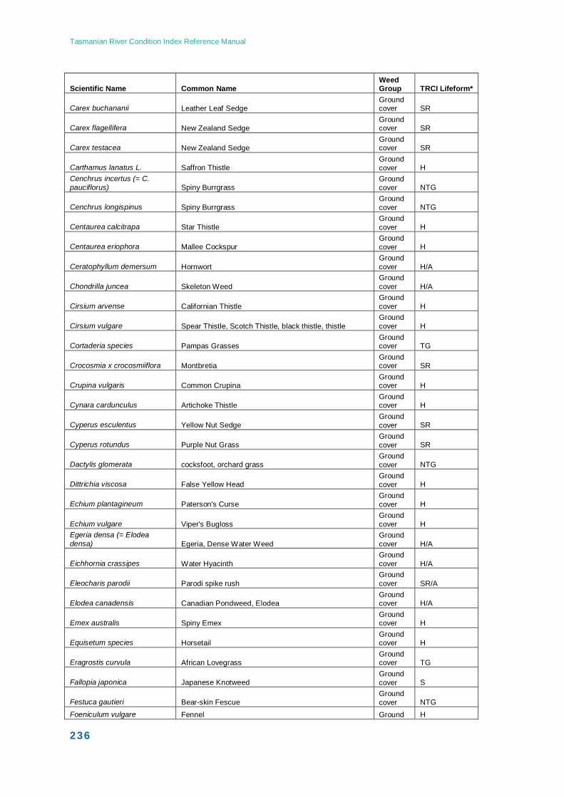
Tasmanian River Condition Index Reference Manual
236
Scientific Name Common Name Weed Group TRCI Lifeform*
Carex buchananii Leather Leaf Sedge Ground cover SR
Carex flagellifera New Zealand Sedge Ground cover SR
Carex testacea New Zealand Sedge Ground cover SR
Carthamus lanatus L. Saffron Thistle Ground cover H
Cenchrus incertus (= C. pauciflorus) Spiny Burrgrass
Ground cover NTG
Cenchrus longispinus Spiny Burrgrass Ground cover NTG
Centaurea calcitrapa Star Thistle Ground cover H
Centaurea eriophora Mallee Cockspur Ground cover H
Ceratophyllum demersum Hornwort Ground cover H/A
Chondrilla juncea Skeleton Weed Ground cover H/A
Cirsium arvense Californian Thistle Ground cover H
Cirsium vulgare Spear Thistle, Scotch Thistle, black thistle, thistle Ground cover H
Cortaderia species Pampas Grasses Ground cover TG
Crocosmia x crocosmiiflora Montbretia Ground cover SR
Crupina vulgaris Common Crupina Ground cover H
Cynara cardunculus Artichoke Thistle Ground cover H
Cyperus esculentus Yellow Nut Sedge Ground cover SR
Cyperus rotundus Purple Nut Grass Ground cover SR
Dactylis glomerata cocksfoot, orchard grass Ground cover NTG
Dittrichia viscosa False Yellow Head Ground cover H
Echium plantagineum Paterson's Curse Ground cover H
Echium vulgare Viper's Bugloss Ground cover H
Egeria densa (= Elodea densa) Egeria, Dense Water Weed
Ground cover H/A
Eichhornia crassipes Water Hyacinth Ground cover H/A
Eleocharis parodii Parodi spike rush Ground cover SR/A
Elodea canadensis Canadian Pondweed, Elodea Ground cover H/A
Emex australis Spiny Emex Ground cover H
Equisetum species Horsetail Ground cover H
Eragrostis curvula African Lovegrass Ground cover TG
Fallopia japonica Japanese Knotweed Ground cover S
Festuca gautieri Bear-skin Fescue Ground cover NTG
Foeniculum vulgare Fennel Ground H
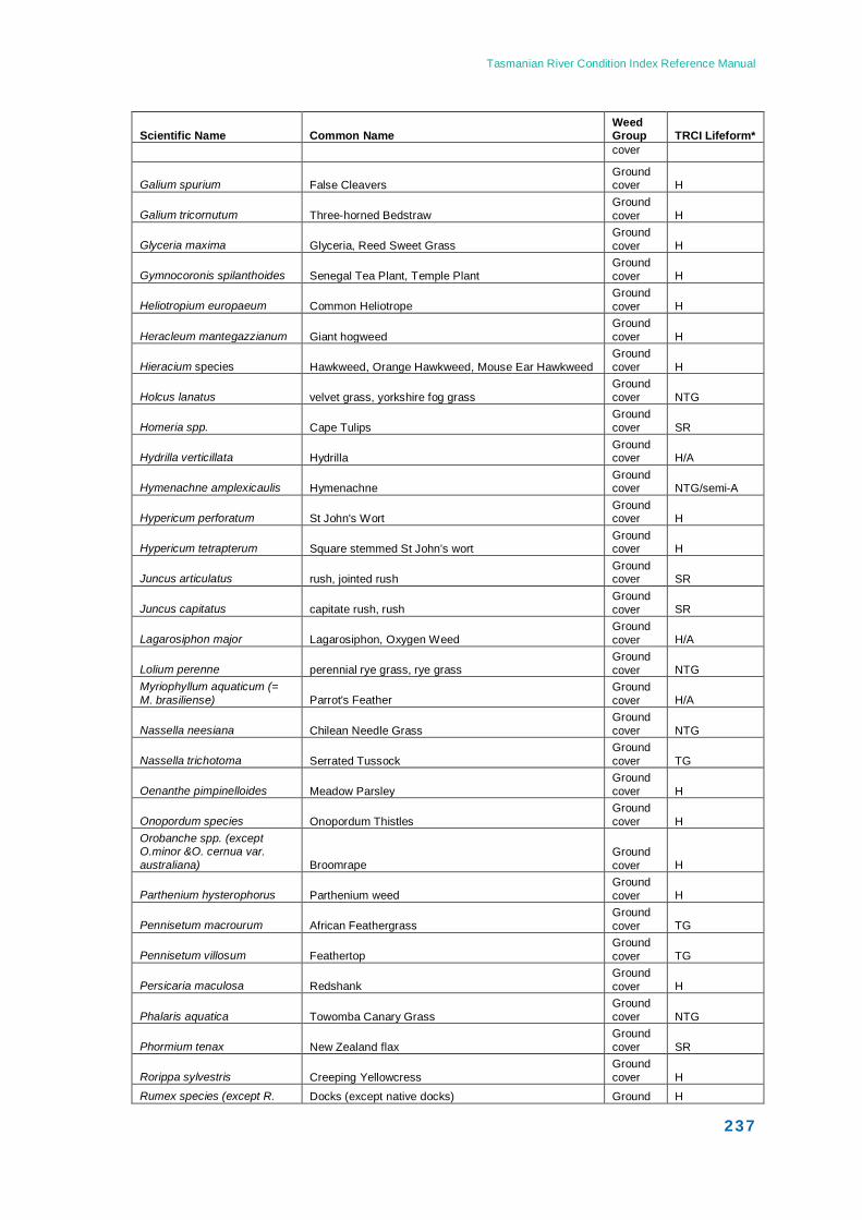
Tasmanian River Condition Index Reference Manual
237
Scientific Name Common Name Weed Group TRCI Lifeform* cover
Galium spurium False Cleavers Ground cover H
Galium tricornutum Three-horned Bedstraw Ground cover H
Glyceria maxima Glyceria, Reed Sweet Grass Ground cover H
Gymnocoronis spilanthoides Senegal Tea Plant, Temple Plant Ground cover H
Heliotropium europaeum Common Heliotrope Ground cover H
Heracleum mantegazzianum Giant hogweed Ground cover H
Hieracium species Hawkweed, Orange Hawkweed, Mouse Ear Hawkweed Ground cover H
Holcus lanatus velvet grass, yorkshire fog grass Ground cover NTG
Homeria spp. Cape Tulips Ground cover SR
Hydrilla verticillata Hydrilla Ground cover H/A
Hymenachne amplexicaulis Hymenachne Ground cover NTG/semi-A
Hypericum perforatum St John's Wort Ground cover H
Hypericum tetrapterum Square stemmed St John’s wort Ground cover H
Juncus articulatus rush, jointed rush Ground cover SR
Juncus capitatus capitate rush, rush Ground cover SR
Lagarosiphon major Lagarosiphon, Oxygen Weed Ground cover H/A
Lolium perenne perennial rye grass, rye grass Ground cover NTG
Myriophyllum aquaticum (= M. brasiliense) Parrot's Feather
Ground cover H/A
Nassella neesiana Chilean Needle Grass Ground cover NTG
Nassella trichotoma Serrated Tussock Ground cover TG
Oenanthe pimpinelloides Meadow Parsley Ground cover H
Onopordum species Onopordum Thistles Ground cover H
Orobanche spp. (except O.minor &O. cernua var. australiana) Broomrape
Ground cover H
Parthenium hysterophorus Parthenium weed Ground cover H
Pennisetum macrourum African Feathergrass Ground cover TG
Pennisetum villosum Feathertop Ground cover TG
Persicaria maculosa Redshank Ground cover H
Phalaris aquatica Towomba Canary Grass Ground cover NTG
Phormium tenax New Zealand flax Ground cover SR
Rorippa sylvestris Creeping Yellowcress Ground cover H
Rumex species (except R. Docks (except native docks) Ground H
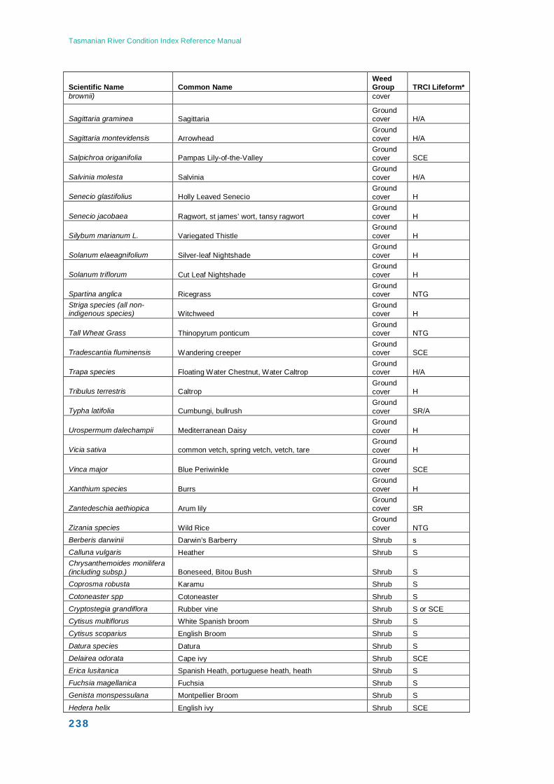
Tasmanian River Condition Index Reference Manual
238
Scientific Name Common Name Weed Group TRCI Lifeform*
brownii) cover
Sagittaria graminea Sagittaria Ground cover H/A
Sagittaria montevidensis Arrowhead Ground cover H/A
Salpichroa origanifolia Pampas Lily-of-the-Valley Ground cover SCE
Salvinia molesta Salvinia Ground cover H/A
Senecio glastifolius Holly Leaved Senecio Ground cover H
Senecio jacobaea Ragwort, st james’ wort, tansy ragwort Ground cover H
Silybum marianum L. Variegated Thistle Ground cover H
Solanum elaeagnifolium Silver-leaf Nightshade Ground cover H
Solanum triflorum Cut Leaf Nightshade Ground cover H
Spartina anglica Ricegrass Ground cover NTG
Striga species (all non-indigenous species) Witchweed
Ground cover H
Tall Wheat Grass Thinopyrum ponticum Ground cover NTG
Tradescantia fluminensis Wandering creeper Ground cover SCE
Trapa species Floating Water Chestnut, Water Caltrop Ground cover H/A
Tribulus terrestris Caltrop Ground cover H
Typha latifolia Cumbungi, bullrush Ground cover SR/A
Urospermum dalechampii Mediterranean Daisy Ground cover H
Vicia sativa common vetch, spring vetch, vetch, tare Ground cover H
Vinca major Blue Periwinkle Ground cover SCE
Xanthium species Burrs Ground cover H
Zantedeschia aethiopica Arum lily Ground cover SR
Zizania species Wild Rice Ground cover NTG
Berberis darwinii Darwin’s Barberry Shrub s Calluna vulgaris Heather Shrub S Chrysanthemoides monilifera (including subsp.) Boneseed, Bitou Bush Shrub S Coprosma robusta Karamu Shrub S
Cotoneaster spp Cotoneaster Shrub S Cryptostegia grandiflora Rubber vine Shrub S or SCE Cytisus multiflorus White Spanish broom Shrub S Cytisus scoparius English Broom Shrub S
Datura species Datura Shrub S Delairea odorata Cape ivy Shrub SCE Erica lusitanica Spanish Heath, portuguese heath, heath Shrub S Fuchsia magellanica Fuchsia Shrub S Genista monspessulana Montpellier Broom Shrub S
Hedera helix English ivy Shrub SCE
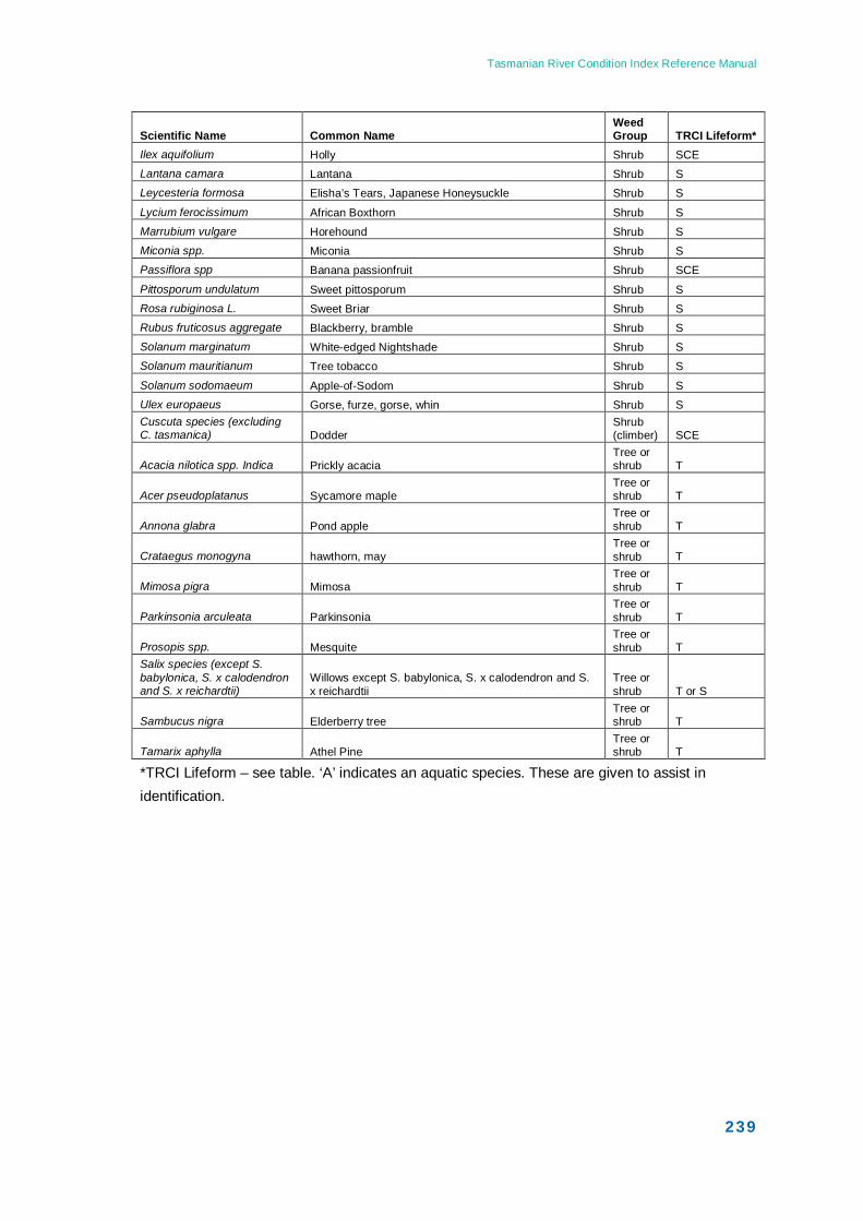
Tasmanian River Condition Index Reference Manual
239
Scientific Name Common Name Weed Group TRCI Lifeform*
Ilex aquifolium Holly Shrub SCE Lantana camara Lantana Shrub S Leycesteria formosa Elisha’s Tears, Japanese Honeysuckle Shrub S
Lycium ferocissimum African Boxthorn Shrub S Marrubium vulgare Horehound Shrub S Miconia spp. Miconia Shrub S Passiflora spp Banana passionfruit Shrub SCE
Pittosporum undulatum Sweet pittosporum Shrub S Rosa rubiginosa L. Sweet Briar Shrub S Rubus fruticosus aggregate Blackberry, bramble Shrub S Solanum marginatum White-edged Nightshade Shrub S Solanum mauritianum Tree tobacco Shrub S
Solanum sodomaeum Apple-of-Sodom Shrub S Ulex europaeus Gorse, furze, gorse, whin Shrub S Cuscuta species (excluding C. tasmanica) Dodder
Shrub (climber) SCE
Acacia nilotica spp. Indica Prickly acacia Tree or shrub T
Acer pseudoplatanus Sycamore maple Tree or shrub T
Annona glabra Pond apple Tree or shrub T
Crataegus monogyna hawthorn, may Tree or shrub T
Mimosa pigra Mimosa Tree or shrub T
Parkinsonia arculeata Parkinsonia Tree or shrub T
Prosopis spp. Mesquite Tree or shrub T
Salix species (except S. babylonica, S. x calodendron and S. x reichardtii)
Willows except S. babylonica, S. x calodendron and S. x reichardtii
Tree or shrub T or S
Sambucus nigra Elderberry tree Tree or shrub T
Tamarix aphylla Athel Pine Tree or shrub T
*TRCI Lifeform – see table. ‘A’ indicates an aquatic species. These are given to assist in identification.
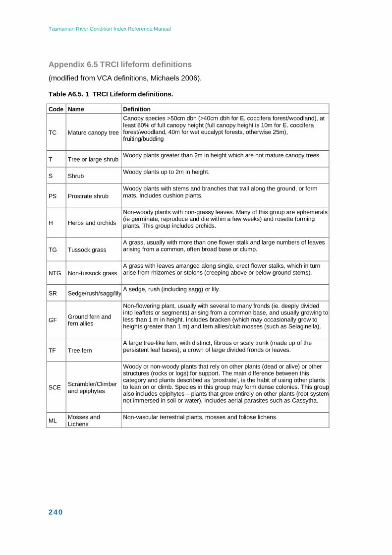
Tasmanian River Condition Index Reference Manual
240
Appendix 6.5 TRCI lifeform definitions (modified from VCA definitions, Michaels 2006).
Table A6.5. 1 TRCI Lifeform definitions.
Code Name Definition
TC Mature canopy tree
Canopy species >50cm dbh (>40cm dbh for E. coccifera forest/woodland), at least 80% of full canopy height (full canopy height is 10m for E. coccifera forest/woodland, 40m for wet eucalypt forests, otherwise 25m), fruiting/budding
T Tree or large shrub Woody plants greater than 2m in height which are not mature canopy trees.
S Shrub Woody plants up to 2m in height.
PS Prostrate shrub Woody plants with stems and branches that trail along the ground, or form mats. Includes cushion plants.
H Herbs and orchids
Non-woody plants with non-grassy leaves. Many of this group are ephemerals (ie germinate, reproduce and die within a few weeks) and rosette forming plants. This group includes orchids.
TG Tussock grass A grass, usually with more than one flower stalk and large numbers of leaves arising from a common, often broad base or clump.
NTG Non-tussock grass A grass with leaves arranged along single, erect flower stalks, which in turn arise from rhizomes or stolons (creeping above or below ground stems).
SR Sedge/rush/sagg/lily A sedge, rush (including sagg) or lily.
GF Ground fern and fern allies
Non-flowering plant, usually with several to many fronds (ie. deeply divided into leaflets or segments) arising from a common base, and usually growing to less than 1 m in height. Includes bracken (which may occasionally grow to heights greater than 1 m) and fern allies/club mosses (such as Selaginella).
TF Tree fern A large tree-like fern, with distinct, fibrous or scaly trunk (made up of the persistent leaf bases), a crown of large divided fronds or leaves.
SCE Scrambler/Climber and epiphytes
Woody or non-woody plants that rely on other plants (dead or alive) or other structures (rocks or logs) for support. The main difference between this category and plants described as ‘prostrate’, is the habit of using other plants to lean on or climb. Species in this group may form dense colonies. This group also includes epiphytes – plants that grow entirely on other plants (root system not immersed in soil or water). Includes aerial parasites such as Cassytha.
ML Mosses and Lichens
Non-vascular terrestrial plants, mosses and foliose lichens.
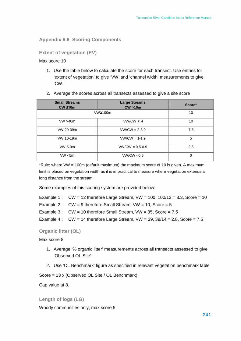
Tasmanian River Condition Index Reference Manual
241
Appendix 6.6 Scoring Components
Extent of vegetation (EV) Max score 10
1. Use the table below to calculate the score for each transect. Use entries for ‘extent of vegetation’ to give ‘VW’ and ‘channel width’ measurements to give ‘CW.’
2. Average the scores across all transects assessed to give a site score
Small Streams CW ≤10m
Large Streams CW >10m Score*
VW≥100m 10
VW >40m VW/CW ≥ 4 10
VW 20-39m VW/CW = 2-3.9 7.5
VW 10-19m VW/CW = 1-1.9 5
VW 5-9m VW/CW = 0.5-0.9 2.5
VW <5m VW/CW <0.5 0
*Rule: where VW = 100m (default maximum) the maximum score of 10 is given. A maximum limit is placed on vegetation width as it is impractical to measure where vegetation extends a long distance from the stream.
Some examples of this scoring system are provided below:
Example 1 : CW = 12 therefore Large Stream, VW = 100, 100/12 = 8.3, Score = 10 Example 2 : CW = 9 therefore Small Stream, VW = 10, Score = 5 Example 3 : CW = 10 therefore Small Stream, VW = 35, Score = 7.5 Example 4 : CW = 14 therefore Large Stream, VW = 39, 39/14 = 2.8, Score = 7.5
Organic litter (OL) Max score 8
1. Average ‘% organic litter’ measurements across all transects assessed to give ‘Observed OL Site’
2. Use ‘OL Benchmark’ figure as specified in relevant vegetation benchmark table
Score = 13 x (Observed OL Site / OL Benchmark)
Cap value at 8.
Length of logs (LG) Woody communities only, max score 5
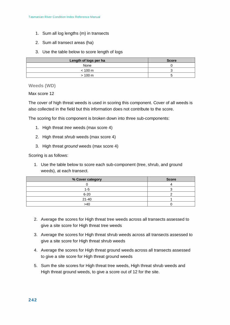
Tasmanian River Condition Index Reference Manual
242
1. Sum all log lengths (m) in transects
2. Sum all transect areas (ha)
3. Use the table below to score length of logs
Length of logs per ha Score None 0
< 100 m 3 > 100 m 5
Weeds (WD) Max score 12
The cover of high threat weeds is used in scoring this component. Cover of all weeds is also collected in the field but this information does not contribute to the score.
The scoring for this component is broken down into three sub-components:
1. High threat tree weeds (max score 4)
2. High threat shrub weeds (max score 4)
3. High threat ground weeds (max score 4)
Scoring is as follows:
1. Use the table below to score each sub-component (tree, shrub, and ground weeds), at each transect.
% Cover category Score 0 4
1-5 3 6-20 2 21-40 1 >40 0
2. Average the scores for High threat tree weeds across all transects assessed to give a site score for High threat tree weeds
3. Average the scores for High threat shrub weeds across all transects assessed to give a site score for High threat shrub weeds
4. Average the scores for High threat ground weeds across all transects assessed to give a site score for High threat ground weeds
5. Sum the site scores for High threat tree weeds, High threat shrub weeds and High threat ground weeds, to give a score out of 12 for the site.
Tasmanian River Condition Index Reference Manual
243
Recruitment (RC) Woody communities only, max score 5
1. Determine the total number of woody species with recruitment in the transects
2. Identify benchmark number of woody species expected to be recruiting from benchmark tables.
Score = 5 x (no. species recruiting on site / benchmark no. of woody species expected to be recruiting).
Cap value at 5.
Tree canopy cover (TC) Forest/woodland communities only, max score 10
1. Average values for tree canopy cover across all transects assessed
2. Identify the expected tree canopy cover from the benchmark
Score =16 x Actual cover/ benchmark cover. Cap at 10.
Number of native species (SP) Max score 10
1. Determine the total number of native species observed in the transects
2. Identify the expected number of species from the benchmark
Score = 10 x (no. native species on site / benchmark no. species). Cap value at 10.
Cover (CO) Max score 10
1. For each lifeform (except mature tree canopy cover), average the cover across all transects assessed to give average ‘observed cover’ per life form code.
2. For each life form, divide ‘observed cover’ by the ‘expected cover’ as specified in the benchmark tables (‘proportion of benchmark present’ column in Table A5.4.4). Cap each value at 1.
3. Add values for each lifeform, divide by the expected number of lifeforms and multiply by 10.
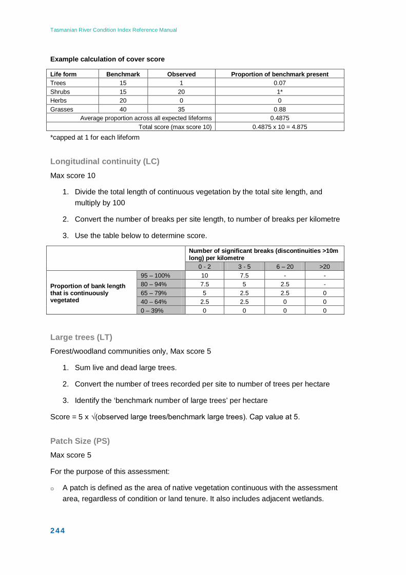
Tasmanian River Condition Index Reference Manual
244
Example calculation of cover score
Life form Benchmark Observed Proportion of benchmark present Trees 15 1 0.07 Shrubs 15 20 1* Herbs 20 0 0 Grasses 40 35 0.88
Average proportion across all expected lifeforms 0.4875 Total score (max score 10) 0.4875 x 10 = 4.875
*capped at 1 for each lifeform
Longitudinal continuity (LC) Max score 10
1. Divide the total length of continuous vegetation by the total site length, and multiply by 100
2. Convert the number of breaks per site length, to number of breaks per kilometre
3. Use the table below to determine score.
Number of significant breaks (discontinuities >10m long) per kilometre
0 - 2 3 - 5 6 – 20 >20
Proportion of bank length that is continuously vegetated
95 – 100% 10 7.5 - - 80 – 94% 7.5 5 2.5 - 65 – 79% 5 2.5 2.5 0 40 – 64% 2.5 2.5 0 0 0 – 39% 0 0 0 0
Large trees (LT) Forest/woodland communities only, Max score 5
1. Sum live and dead large trees.
2. Convert the number of trees recorded per site to number of trees per hectare
3. Identify the ‘benchmark number of large trees’ per hectare
Score = 5 x √(observed large trees/benchmark large trees). Cap value at 5.
Patch Size (PS) Max score 5
For the purpose of this assessment:
o A patch is defined as the area of native vegetation continuous with the assessment area, regardless of condition or land tenure. It also includes adjacent wetlands.
Tasmanian River Condition Index Reference Manual
245
o Native vegetation is defined as vegetation dominated by native species and does not include TASVEG codes FAG, FUM, FMG, FPE, FPL, FPF, FRG, FSM, FUR and FWU.
o A patch has a defined physical boundary such as cleared land. o Vegetation corridors and linkages such as road reserves connecting larger areas of
native vegetation are considered part of the larger patch where they have a minimum width of 50m.
o Vegetation that is contiguous with a larger patch but which is less than 50m wide should be treated as a different patch.
o Waterways are not considered to be a patch boundary unless they are >50m wide o If the vegetation community on site or adjacent to the site is a grassland, the data
sheets will need to be examined to confirm GIS/TASVEG results, as TASVEG may not differentiate between the extent of native and exotic grassland/pasture communities.
Determine the size of the patch using a GIS (e.g. aerial photography, vegetation mapping etc). This will be achieved by drawing a polygon around native vegetation (as described above) that is contiguous with the vegetation at the site start coordinate location and determining its area in hectares.
Score = 0.25 x patch size (ha). Capped at 5.
Neighbourhood Max score 5
For the purpose of this assessment:
o Native vegetation includes any vegetation community regardless of type, condition or tenure and can also include natural wetlands, lakes (i.e. not artificial impoundments), estuaries and rivers.
o When assessing near coastal vegetation, the shape of the neighbourhood boundaries should be adjusted to coincide with the low tide mark thus excluding the open sea/ocean.
o If the vegetation community on site or adjacent to the site is a grassland, the data sheets will need to be examined to confirm GIS/TASVEG results, as TASVEG may not differentiate between the extent of native and exotic grassland/pasture communities.
Assessment and scoring is as follows:
1. Draw three circles (100m, 1 km and 5km radii) around the measuring site, centred upon the site start co-ordinate. Estimate the percentage of native vegetation in each circle and round up or down to the nearest 20%.
Tasmanian River Condition Index Reference Manual
246
2. Assign the appropriate category and score as shown in the table below.
3. Multiply % native vegetation x weighting for each radius from the zone then add values to obtain final Neighbourhood Value.
Radius from Site % Native Vegetation* Weighting Result 100m 0.015 1km 0.02 5km 0.015
Add values and round off
* to the nearest 20%
Distance to Core Area Max score 5
This component is assessed by measuring the distance to the nearest ‘core area’ which is defined as any patch of native vegetation greater than 50ha regardless of type, condition or tenure. This includes natural wetlands, lakes (i.e. not artificial impoundments), estuaries and rivers. The open sea/ocean is not considered native vegetation.
If the vegetation community on site or adjacent to the site is a grassland, the data sheets will need to be examined to confirm GIS/TASVEG results, as TASVEG may not differentiate between the extent of native and exotic grassland/pasture communities.
As with the neighbourhood component, which is measured from the site start coordinate position, distance to core area is measured to the closest edge of the core area.
Score = 5 – (0.5 x distance to core area(km)). Minimum zero.
Tasmanian River Condition Index Reference Manual
247
7 Water Quality Sub-Index
7.1 Introduction A Water Quality sub-index was originally recommended for inclusion in the TRCI but was not pursued. In 2007, a draft method was developed that recommended assessing changes to sediment and nutrient loads in rivers. It was proposed that that use of SedNet to model sediment and nutrient loads in rivers be trialled, rather than undertaking water quality monitoring to obtain this information. Model outputs were to be validated using targeted campaigns of water quality monitoring. This trial did not go ahead due to budgetary constraints (Earth Tech 2007b).
The TRCI has been designed so that a Water Quality sub-index could be included in the future once a suitable approach is trialled and confirmed.
7.2 Developing the Draft Method A review of potential water quality parameters for inclusion in the TRCI found that sediment and nutrients were the most appropriate for inclusion in a state-wide assessment of condition (Earth Tech 2007). Unlike point source pollutants (such as heavy metal contaminants) and salinity, sediment and nutrients are relevant in the majority of catchments in Tasmania and respond to changes in land use and riparian management within a catchment. It was considered that local point source issues were best examined through targeted studies rather than a broad, catchment or regional scale assessment program like the TRCI (Earth Tech 2007b).
Water quality sampling (spot measurement) was considered for use in the TRCI to provide catchment-wide assessments of water quality. Although often the most intuitive approach, sampling is expensive as numerous sites are required (over time and within a catchment) if reasonable statistical power is to be achieved. An initial review of water quality monitoring in Tasmania showed that only limited data were available (Earth Tech 2007b). Approximately 38 sites in Tasmania had water quality data suitable for use in the TRCI, although nutrient data was not collected at some of these sites. Significant resources (beyond those of the TRCI) would be required to establish an adequate number of measurement sites over the large spatial and temporal scales required for TRCI. The interpretation and transformation of water quality measures into objective condition scores would also require significant resources (Earth Tech 2007b).
As an alternative, it was recommended that a spatial modelling approach be adopted for the TRCI, combined with limited water quality monitoring to validate and improve the model. Assessments using a spatial modelling approach could be made at the catchment or regional scale and pre-European reference conditions would be identified
Tasmanian River Condition Index Reference Manual
248
using modelled data. Additionally, a modelling approach could potentially identify the sources of sediment and nutrients and likely causes of degradation (eg. poor riparian vegetation, bank, bed or hillslope stability, land use change).
Both E2 and SedNet models were considered to provide the spatial modelling of sediment and nutrients for the water quality assessments of the TRCI (Earth Tech 2007b). Each modelling approach had a number of limitations, however, on balance SedNet was recommended for ease of use and data requirements were less expensive (Earth Tech 2007b).
However, one of the major concerns with adopting a spatial modelling approach was the initial cost associated with setting up the models. The resources required to conduct a pilot study using SedNet were estimated by Earth Tech (2007b). The collection of input data for regional models, model operation, reporting, mapping, training and additional field data collection, required approximately 17-18 weeks work by one person to complete them. The project team discussed these costs and decided instead to commission a detailed investigation of the feasibility of using SedNet to assess water quality in the TRCI.
The feasibility report suggested that SedNet would be appropriate to use at the regional level, rather than the catchment scale, but that the model was yet to be rigorously tested in Tasmania (Earth Tech 2007c). A pilot application of SedNet was recommended for the North East region of the state, with the outcomes guiding further modelling throughout Tasmania (Earth Tech 2007c).
The North East region was suggested for the trial as it had the greatest density of streamflow gauges and coverage of aerial photographs. A number of catchments in the region had been included in State of the River reporting. The North East also included the South Esk catchment which had been previously modelled (S. Lynch, pers comm). The trial would include:
o developing missing datasets; o running the model for the current landuse scenario; o checking the model outputs against observed loads; o developing and testing scenarios (Earth Tech 2007c).
As well as assessing the effectiveness of the SedNet model in detecting trends in water quality, the trial would enable methods for collecting missing data and collating existing data to be developed. Upon completion of the trial, SedNet could be applied to other regions where data is more limited. It was anticipated that the trial would cost in the order of $50,000 (Earth Tech 2007c).
If the trial was successful, it was suggested that Tasmania would best be modelled as four regions (north west, north east, west / south west and south east) and that each region could cost up to $50,000 to model initially. Ongoing modelling within the recommended timeframe (approximately every 5-10 years) of the TRCI would be
Tasmanian River Condition Index Reference Manual
249
considerably cheaper (<$10,000), as the models would already be established (Earth Tech 2007c).
7.3 Status of the Water Quality sub-index The cost of completing the SedNet trial in the North East was beyond the budget of the TRCI project. The $50,000 required for the SedNet trial would have severely reduced the resources available to trial the remaining methods. The project team, including the expert panel and the Tasmanian NRMs, agreed to place the Water Quality sub-index on hold.
Although the Framework for Assessment of River and Wetland Health (FARWH) includes water quality as key criteria for assessing river condition, it is well recognised nationally that adequate water quality monitoring is challenging. The Murray Darling Basin Authority’s SRA pilot suggested that water quality would not be included in the final SRA due to spatial and temporal variability and the difficulty in defining reference conditions. Like the TRCI, this program currently has a ‘watching brief’ over water quality.
Although the TRCI may give a more complete indication of river condition if a dedicated water quality index were included, it is anticipated that some existing components of the other sub-indices may indicate water quality changes. For example:
o Reduced diversity and abundance of macroinvertebrates and increased algae, (Aquatic Life sub-index) may indicate increased nutrient, sediment and other pollutants.
o Increased fine sediment accumulation (Physical form sub-index) could indicate elevated sediment loads in the rivers.
o Increased coverage of instream macrophytes (Physical form sub-index) may indicate increased sediment and nutrients.
The TRCI has been designed so that should resources become available, or further developments in the assessment of water quality occur, a Water Quality sub-index could be incorporated into the TRCI framework. A project currently being managed by NRM North (as part of the Tamar Estuary Esk Rivers project) is using E2 to model nutrient and sediment levels. The outcomes of this project could inform future development of a Water Quality sub-index.
The Tasmanian River Condition Index recommended approach (Earth Tech 2007a), draft method (Earth Tech 2007b) and Water Quality sub-index feasibility report (Earth Tech 2007c) are available from NRM South.
Tasmanian River Condition Index Reference Manual
250
7.4 References - Water Quality Earth Tech (2007a) River Condition Index for Tasmania: Recommended Approach. A report to NRM South. Earth Tech, Wangaratta, Victoria.
Earth Tech (2007b) River Condition Index for Tasmania: Draft Method for Testing. A report to NRM South. Earth Tech, Wangaratta, Victoria.
Earth Tech (2007c) The Feasibility of Using SedNet to Assess Water Quality in the Tasmanian River Condition Index. A report to NRM South. Earth Tech, Townsville, Queensland.


