NBER WORKING PAPER SERIES

SWEAT EQUITY IN U.S. PRIVATE BUSINESS

Anmol BhandariEllen R. McGrattan

Working Paper 24520http://www.nber.org/papers/w24520

NATIONAL BUREAU OF ECONOMIC RESEARCH1050 Massachusetts Avenue

Cambridge, MA 02138April 2018, Revised January 2020

Bhandari acknowledges support from the Heller-Hurwicz Economic Institute, and McGrattan ac- knowledges support from the NSF. Replication codes and data are available at www.econ.umn.edu/~erm/data/sweat. We thank Yuki Yao for excellent research assistance and James Holt for excel- lent editorial assistance. We thank V.V. Chari, Bob Hall, Ed Prescott, and seminar participants at the University of Colorado, the University of Minnesota, Yale, Autonoma, ASU, NYU, Columbia, the Bank of Korea, the SED, Stanford, CMU, and the EUI for helpful comments. The views expressed herein are those of the authors and not necessarily those of the Federal Reserve Bank of Minneapolis, the Federal Reserve System, or the National Bureau of Economic Research.

NBER working papers are circulated for discussion and comment purposes. They have not been peer-reviewed or been subject to the review by the NBER Board of Directors that accompanies official NBER publications.

© 2018 by Anmol Bhandari and Ellen R. McGrattan. All rights reserved. Short sections of text, not to exceed two paragraphs, may be quoted without explicit permission provided that full credit, including © notice, is given to the source.

Sweat Equity in U.S. Private Business Anmol Bhandari and Ellen R. McGrattan NBER Working Paper No. 24520April 2018, Revised January 2020JEL No. E13,E22,H25

ABSTRACT

We develop a theory of sweat equity—the value of business owners’ time and expenses to build customer bases, client lists, and other intangible assets. We discipline the theory using data from U.S. national accounts, business censuses, and brokered sales to estimate a value for sweat equity for the private business sector equal to 1.2 times U.S. GDP, which is roughly the value of fixed assets in use in these businesses. Although latent, the equity values are positively correlated with business incomes, ages, and standard measures of markups based on accounting data, but not with financial assets of owners or standard measures of business total factor productivity (TFP). We use our theory to show that abstracting from sweat activity leads to a significant understatement of the impacts of lowering business income tax rates on both the extensive and intensive margins. We also document large differences in the effective tax rates and the effects of tax changes for owner and employee labor inputs. Lower tax rates on owners result in increased self-employment rates and smaller firm sizes, whereas lower rates on employees have the opposite effect. Allowing for financial constraints and superstar firms does not overturn our main findings.

Anmol BhandariDepartment of EconomicsUniversity of Minnesota1925 Fourth Street SouthMinneapolis, MN 55455and NBERbhandari@umn.edu

Ellen R. McGrattanDepartment of EconomicsUniversity of Minnesota4-101 Hanson Hall1925 4th St SMinneapolis, MN 55455and NBERerm@umn.edu

1. Introduction

Private businesses in the United States now account for over 60 percent of yearly business net

income.1 Empirical evidence suggests that a significant part of this income is compensation for time

that owners devote to building sweat equity in their business in the form of valuable client lists,

customer bases, brands, and other intangible assets. Beyond providing current income to owners,

these investments also generate capital gains when the business is eventually sold and intangible

capital is transferred. Because standard theories in public finance abstract from sweat equity, they

miss potentially important margins of substitution in response to both business and labor tax

reforms. In this paper, we develop a theory in which this investment is a central feature and use

it, along with U.S. national accounts and business census microdata, to measure net incomes and

sweat equity in private business. Once measured, we quantify its role for tax policy reform.

As evidence of the labor content of business income, Smith et al. (2019) use tax filings to show

that business income falls substantially after owner retirements and premature deaths, implying

that much of the income is a return on the owner’s time. Aggregating across pass-through entities,

they estimate that three-quarters of the business profits are actually payments to labor.2 If the

payments were purely compensation to nontransferable human capital, at the time a business

sells, we would observe that only financial and fixed assets are transferred. Instead, using data

from brokered sales compiled by Pratt’s Stats, we find that a large fraction of transferred assets

are categorized by the Internal Revenue Service (IRS) as Section 197 intangible assets. These

assets include customer- and information-based intangibles, trademarks, trade names, franchises,

contracts, patents, copyrights, formulae, processes, designs, patterns, noncompete agreements,

licenses, permits, and goodwill. We use a sample of 6,855 sales of private businesses over the

period 1994–2017 to construct ratios of intangible asset values to the total assets—what we call

the intangible intensity. We find an average intensity of 58 percent and a median of 64 percent.

The remaining value is attributed to cash, trade receivables, inventories, fixed assets, and real

1 Bhandari et al. (2019) document a 60.6 percent share of taxable net income and a 65.5 percent share ofpost-audit net income for private U.S. businesses over the period 2004–2014.

2 Most private businesses are pass-through entities—sole proprietorships, S corporations, or partnerships—thatdistribute all earnings to owners. They report business net incomes on their individual tax returns and accountfor 57 percent of post-audit business net income over the period 2004–2014. See also Koh, Santaeulalia-Llopis,and Zheng (2018), who provide evidence of a stable U.S. labor share after recategorizing part of business profitsas labor compensation.

1

estate. These estimates are robust to conditioning on legal structure, industry, and firm size. (See

Bhandari and McGrattan 2019 for full details.)

To measure these intangible assets for ongoing concerns, we develop a dynamic general equi-

librium lifecycle model with privately and publicly held businesses. We explicitly model the time

use of private business owners. Besides leisure, they put time into two activities: production of

goods and services and accumulation of sweat capital, which consists of building their client lists,

customer bases, goodwill, and so on. Sweat capital is an input of production, along with tangible

capital, owner hours, and employee hours. The income generated from sweat capital can be thought

of as dividends whose present value is the sweat equity we are interested in measuring. During

each period over their life cycle, individuals choose to run their own business or work for another

business—either private or public—with this occupational choice driven primarily by stochastic

productivities in each activity, accumulated sweat capital, and tax policy. We assume nonsweat

capital can be rented and external labor hired, and therefore the main start-up costs are the time

and expenses of the owner for accumulating sweat capital, an asset that is not pledgeable.

To parameterize the model, we use aggregate data from the U.S. national income and product

accounts (NIPA), panel data of business incomes and wages from the IRS, cross-sectional data

on business ages and owner hours from the U.S. Census Survey of Business Owners (SBO), and

intangible share of business valuations from Pratt’s Stats. Two key parameters in our model

that have not been estimated in other studies are the share of sweat capital in private business

production and the deterioration of this capital when the current owner is not actively using it.

These parameters are identified by matching model and data intangible intensities and business

age profiles. Also novel here is the estimation of private business owners’ labor income as a share

of GDP using data from NIPA and the IRS. This exercise is relatively straightforward for pass-

through business owners, for whose income we estimate a share of 9 percent of GDP. Imputations

are needed in the case of private C corporation owners, for whose income we estimate a share of

roughly 2 percent of GDP. The present value of this labor income is partly a wage payment for

time in production and partly the value of the intangible assets in the business.

Conceptually, our measure of sweat equity is the shadow value for a hypothetical mutual fund

that passively invests in all potential private business owners, reaping the net returns after paying

2

owners for their labor in producing private goods and services. For all private businesses, we

estimate an aggregate sweat equity value of 1.2 times GDP, which is roughly equal to the value

of tangible assets in use in these businesses and about 84 percent of the market capitalization of

publicly held corporations. This measure includes both transferable wealth in the form of sweat

capital and nontransferable wealth in the form of an owner-specific endowment of productivity to

run a business. Values reported in brokered sales or business surveys would include only transferable

assets. To estimate this value for ongoing concerns, we survey owners in our model at a point in

time and ask at what price they would be willing to sell the transferable sweat capital. We find

an average value for current owners that is 30 percent of the sweat equity value. We also find that

the dispersion in this estimate of wealth is far greater than in that of sweat equity values.

Although we cannot directly observe the sweat capital or the implied sweat equity of ongoing

businesses, the latent capital stocks are positively correlated with some observable variables that

could serve as useful proxies. For example, we find that the sweat capital is positively correlated

with business incomes and ages, since production cannot occur without clients or customers. Sweat

capital is also positively correlated with standard measures of markups—sales relative to variable

costs—if expenses are incurred when building the client list. This is true even though there are no

actual markups in the baseline model. We find a negative correlation with standard measures of

TFP that only count the tangible capital stocks and no relation with financial assets even when

we allow for working capital constraints.

We investigate the quantitative role of including owner time in production and sweat capital

accumulation for the study of business taxation. Specifically, we compare the predictions of lowering

taxes on incomes of privately and publicly held businesses in our baseline model to those of a nested

model in which owner time is fixed and there is no sweat capital. This nested model is the span-

of-control model of Lucas (1978), which has become the standard framework in the literature on

entrepreneurial choice. As compared with no-sweat, Lucas type models, we find much larger effects

of lowering tax on private businesses in our baseline model. The no-sweat model has a negligible

intensive margin effect because a tax on business income ultimately falls on the return to a fixed

managerial input and hence is not distortive. Introducing sweat, we find a large effect on the

intensive margin as owners work longer hours and hire less outside labor. Despite these large

3

effects, we find the short-run responses and implied labor-supply elasticities of most owners in line

with empirical estimates. There are two main reasons for this result. First, owner time in our

model is a non-traded input, and hence the shadow wage (proxied by the disutility of supplying

hours) suffers a larger adverse incidence when taxes are lowered and owners work more. Second,

owners can increase production hours by spending less time building sweat capital. Even on the

extensive margin, we find larger effects than in Lucas (1978). Allowing for sweat investment leads

to increased returns in other factors and amplifies incentives to enter when taxes on businesses

incomes are lowered.

If we additionally lower tax rates on corporate profits, then we find larger responses for the

effects on the private business sector across the models with and without sweat activity but similar

predictions for the effects on the C-corporate sector and aggregated data. Across the business

owners, we find that most of the changes are attributed to businesses that have high productivities

and large sweat capital stocks. Although true productivities are exogenous and true markups are

constant, standard measures of total factor productivities and markups are significantly higher

after the tax change.

Since private business income is primarily labor income, we compare the economic effects of

taxing owner net incomes versus employee earnings. Lowering tax rates on owner time leads to a

shift in the business labor force: owners put in more of their own time producing goods and services

and hire fewer paid employees. In effect, the tax change results in more firms that are smaller in

scale. Lowering tax rates on employee time leads to fewer owners since owners can make more

working for someone else. However, the owners that find paid employment more attractive are

not the most productive in business. Even with lower taxes on paid employment, the very highly

productive owners would still find it optimal to run a business. With fewer owners and continued

demand for the goods they produce, relative prices rise, and more outside labor and capital are

used to meet that demand. In effect, the tax change results in fewer firms that are larger in scale.

Our paper is related to studies of small businesses and entrepreneurship. There are now many

quantitative theories of entrepreneurship. Most model entrepreneurs as owners of physical capital

subject to uninsurable idiosyncratic risk and financing constraints. See, for example, Angeletos

and Calvet (2006), Boar and Midrigan (2019), Buera (2009), Cagetti and De Nardi (2006), Dyrda

4

and Pugsley (2017), Li (2002), Meh (2005), Peter (2019), and Quadrini (1999, 2000). These studies

focus mainly on the role of financial frictions in accounting for dispersion in survey-based measures

of wealth and income.3 We include working capital constraints disciplined by estimates of available

funds to value added but find they have a negligible effect on the results our tax analyses. We also

include superstar firms—whose owners earn 10 times the median labor income—and the model can

generate large wealth ginis without assuming extreme productivity differences in the distribution.

(See Castaneda, Diaz-Gimenez, and Rios-Rull, 2003.)

Another related line of research models entrepreneurial choices as driven by the nonpecuniary

benefits of owning a business. See, for example, Hamilton (2000), Moskowitz and Vissing-Jorgensen

(2002), Hall andWoodward (2010), and Hurst and Pugsley (2011, 2017). This literature is informed

by survey responses of small-business owners and evidence that these owners have lower accumu-

lated earnings over time than they would have had if they had worked for someone else and made

fewer risky investments. We find that differences in the effective marginal tax rates of business

owners and wage earners can account for almost all differences in pre-tax earnings. Thus, alter-

ing preferences to include a role for nonpecuniary benefits does not alter our main quantitative

findings.

None of the studies on entrepreneurial choice explicitly model the accumulation of the business

owner’s sweat in building the business and therefore cannot be used to estimate aggregate or cross-

sectional valuations of this key business asset or its role for tax policy reform.4

2. Theory

In this section, we develop a theory to measure sweat equity in private businesses and to serve

as a tool for the study of tax policy counterfactuals. We start with an overview of the environment

3 The literature on factor misallocation uses similar theories of entrepreneurs to quantify cross-country differencesin aggregate productivity. See, for example, Buera and Shin (2013), Midrigan and Xu (2014), and Restucciaand Rogerson (2008), as well as Hopenhayn’s (2014) survey for a complete list of references.

4 In other literatures, researchers model investments in intangible capital—including brand and customer capital—to study trade patterns, asset pricing, firm dynamics, and business cycles, but they do not model the time-usedecisions of private business owners. See, for example, Arkolakis (2010), Atkeson and Kehoe (2005), Belo,Lin, and Vitorino (2014), Drozd and Nosal (2012), Gourio and Rudanko (2014), and McGrattan and Prescott(2010a,2010b).

5

and then turn to a full description of the dynamic programs solved by different agents in the

economy.

2.1. Overview

The economy is populated with individuals who age stochastically and are endowed with skills

that govern their productivities in running businesses and paid employment. Over the life cycle,

they make occupational choices: they earn either wage income as employees or business income as

owners of private firms.

We assume that there are two business sectors: publicly held C corporations and privately held

pass-through businesses that sell goods and services.5 Businesses in the two sectors differ in their

technologies, exposure to idiosyncratic risk, and tax treatment. Moreover, the goods produced in

the two sectors are imperfectly substitutable.

Publicly held C corporations are assumed have fully diversified ownership. They use fixed

assets as well as the time of paid employees as inputs to a constant-returns production technology.

Their owners are assumed to be outside shareholders who do not work in the business. In the case

of private firms, owners bear idiosyncratic risk and put time into producing goods and services

and into building sweat capital—the business customer base, client list, and other non-pledgeable

intangible assets.6 In addition to owner sweat, private firms use fixed assets and time of paid

employees.

Business incomes in the two sectors face different tax treatment. C corporations pay corporate

income tax on profits, and the shareholders pay individual income tax on any distributions, while

pass-through entities distribute all profits to their owners, who pay individual income taxes on the

proceeds.

There is a competitive intermediation sector with risk-neutral financial intermediaries, who

5 In the United States, there are privately-held C corporations for which we have very limited data from theIRS. When calibrating the model, we separate businesses into C corporations and pass-through businesses, butlater use the limited data that we have to impute sweat equity valuations for privately-held C corporations.

6 Much of C-corporate intangible investment does show up in the national accounts as intermediate purchasesor employee compensation. A good example of the latter is wage compensation to R&D scientists.

6

accept deposits and use the funds to purchase equities of publicly held firms and government bonds

and fixed assets that they rent to private firms.

Finally, there is a nonbusiness sector that includes production by the government, households,

and nonprofit institutions that primarily serve households. Government purchases are financed by

taxes on consumption, individual incomes, and business incomes.

We next turn to a formal description of this environment.

2.2. Occupational Choice

At a point in time, the state vector s for any individual—whether an entrepreneur or an

employee—includes financial assets a, sweat capital κ, the productivity of working for someone else

ǫ, the productivity of running a business z, and age j. The occupational choice of an individual is

made to maximize the overall value:

Vj (s) = max{Vj,p (s) , Vj,w (s)},

where Vj,p(s) is the value to running one’s own private business, and Vj,w(s) is the value to working

for those in age group j. To keep the life cycle problems tractable, we allow for stochastic aging

between young ages, j = y, and old ages, j = o as in Blanchard (1985). We also assume that

individuals spend some fraction of their life in paid employment and another in self-employment;

the spells do not overlap. In reality, some individuals do both activities simultaneously: they work

for someone else and run a business. However, data on time use show that average hours on the

primary job are much higher than on the secondary job.

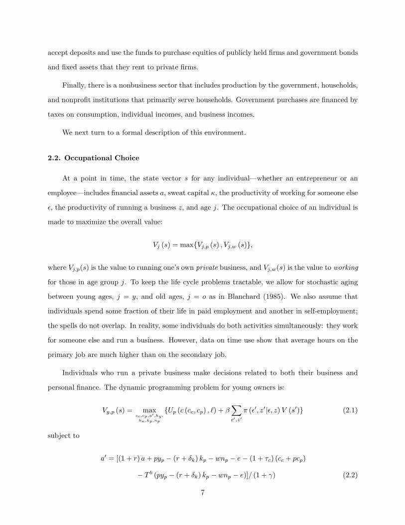
Individuals who run a private business make decisions related to both their business and

personal finance. The dynamic programming problem for young owners is:

Vy,p (s) = maxcc,cp,a′,hy,

hκ,kp,np

{Up (c (cc, cp) , ℓ) + β∑

ǫ′,z′

π (ǫ′, z′|ǫ, z) V (s′)} (2.1)

subject to

a′ = [(1 + r) a+ pyp − (r + δk) kp − wnp − e− (1 + τc) (cc + pcp)

− T b (pyp − (r + δk) kp − wnp − e)]/ (1 + γ) (2.2)

7

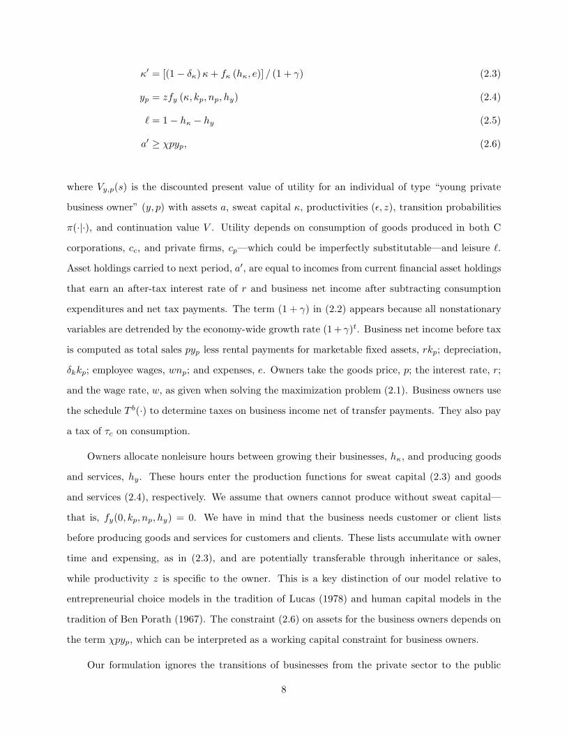
κ′ = [(1− δκ)κ+ fκ (hκ, e)] / (1 + γ) (2.3)

yp = zfy (κ, kp, np, hy) (2.4)

ℓ = 1− hκ − hy (2.5)

a′ ≥ χpyp, (2.6)

where Vy,p(s) is the discounted present value of utility for an individual of type “young private

business owner” (y, p) with assets a, sweat capital κ, productivities (ǫ, z), transition probabilities

π(·|·), and continuation value V . Utility depends on consumption of goods produced in both C

corporations, cc, and private firms, cp—which could be imperfectly substitutable—and leisure ℓ.

Asset holdings carried to next period, a′, are equal to incomes from current financial asset holdings

that earn an after-tax interest rate of r and business net income after subtracting consumption

expenditures and net tax payments. The term (1 + γ) in (2.2) appears because all nonstationary

variables are detrended by the economy-wide growth rate (1+ γ)t. Business net income before tax

is computed as total sales pyp less rental payments for marketable fixed assets, rkp; depreciation,

δkkp; employee wages, wnp; and expenses, e. Owners take the goods price, p; the interest rate, r;

and the wage rate, w, as given when solving the maximization problem (2.1). Business owners use

the schedule T b(·) to determine taxes on business income net of transfer payments. They also pay

a tax of τc on consumption.

Owners allocate nonleisure hours between growing their businesses, hκ, and producing goods

and services, hy. These hours enter the production functions for sweat capital (2.3) and goods

and services (2.4), respectively. We assume that owners cannot produce without sweat capital—

that is, fy(0, kp, np, hy) = 0. We have in mind that the business needs customer or client lists

before producing goods and services for customers and clients. These lists accumulate with owner

time and expensing, as in (2.3), and are potentially transferable through inheritance or sales,

while productivity z is specific to the owner. This is a key distinction of our model relative to

entrepreneurial choice models in the tradition of Lucas (1978) and human capital models in the

tradition of Ben Porath (1967). The constraint (2.6) on assets for the business owners depends on

the term χpyp, which can be interpreted as a working capital constraint for business owners.

Our formulation ignores the transitions of businesses from the private sector to the public

8

sector. This is informed by studies of firm dynamics that use panel data (see Cole and Sokolyk

(2018)) and conclude that firms’ choice of the legal form of organization is largely set in stone at

inception. 7

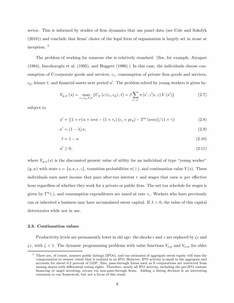
The problem of working for someone else is relatively standard. (See, for example, Aiyagari

(1994), Imrohoroglu et al. (1995), and Huggett (1996).) In this case, the individuals choose con-

sumption of C-corporate goods and services, cc, consumption of private firm goods and services,

cp, leisure ℓ, and financial assets next period a′. The problem solved by young workers is given by:

Vy,w (s) = maxcc,cp,ℓ,a′

{Uw (c (cc, cp) , ℓ) + β∑

ǫ′,z′

π (ǫ′, z′|ǫ, z) V (s′)} (2.7)

subject to

a′ = [(1 + r) a+ wǫn− (1 + τc) (cc + pcp)− Tw (wǫn)]/ (1 + γ) (2.8)

κ′ = (1− λ)κ, (2.9)

ℓ = 1− n (2.10)

a′ ≥ 0, (2.11)

where Vy,w(s) is the discounted present value of utility for an individual of type “young worker”

(y,w) with state s = {a, κ, ǫ, z}, transition probabilities π(·|·), and continuation value V (s). These

individuals earn asset income that pays after-tax interest r and wages that earn w per effective

hour regardless of whether they work for a private or public firm. The net tax schedule for wages is

given by Tw(·), and consumption expenditures are taxed at rate τc. Workers who have previously

run or inherited a business may have accumulated sweat capital. If λ > 0, the value of this capital

deteriorates while not in use.

2.3. Continuation values

Productivity levels are permanently lower in old age: the shocks ǫ and z are replaced by ζǫ and

ζz, with ζ < 1. The dynamic programming problems with value functions Vo,p and Vo,w for older

7 There are, of course, nonzero public listings (IPOs), and our estimates of aggregate sweat equity will miss thecompensation to owners’ sweat that is realized in an IPO. However, IPO activity is small in the aggregate andaccounts for about 0.2 percent of GDP. Also, pass-through forms such as S corporations are restricted fromissuing shares with differential voting rights. Therefore, nearly all IPO activity, including the pre-IPO venturefinancing or angel investing, occurs via non-pass-through firms. Adding a listing decision is an interestingextension to our framework, but not a focus of this study.

9

private business owners and workers are formulated in the same way as for younger individuals

with modified continuation values.

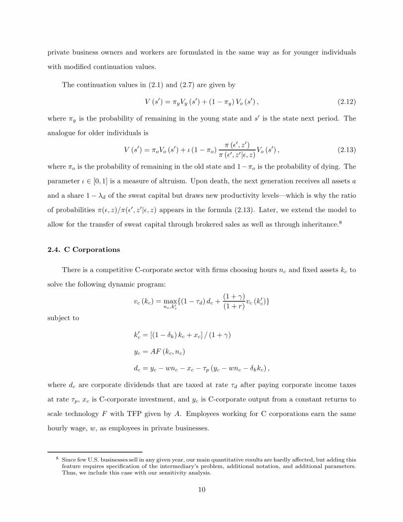
The continuation values in (2.1) and (2.7) are given by

V (s′) = πyVy (s′) + (1− πy)Vo (s

′) , (2.12)

where πy is the probability of remaining in the young state and s′ is the state next period. The

analogue for older individuals is

V (s′) = πoVo (s′) + ι (1− πo)

π (ǫ′, z′)

π (ǫ′, z′|ǫ, z)Vo (s

′) , (2.13)

where πo is the probability of remaining in the old state and 1−πo is the probability of dying. The

parameter ι ∈ [0, 1] is a measure of altruism. Upon death, the next generation receives all assets a

and a share 1− λd of the sweat capital but draws new productivity levels—which is why the ratio

of probabilities π(ǫ, z)/π(ǫ′, z′|ǫ, z) appears in the formula (2.13). Later, we extend the model to

allow for the transfer of sweat capital through brokered sales as well as through inheritance.8

2.4. C Corporations

There is a competitive C-corporate sector with firms choosing hours nc and fixed assets kc to

solve the following dynamic program:

vc (kc) = maxnc,k′

c

{(1− τd) dc +(1 + γ)

(1 + r)vc (k

′

c)}

subject to

k′c = [(1− δk) kc + xc] / (1 + γ)

yc = AF (kc, nc)

dc = yc − wnc − xc − τp (yc − wnc − δkkc) ,

where dc are corporate dividends that are taxed at rate τd after paying corporate income taxes

at rate τp, xc is C-corporate investment, and yc is C-corporate output from a constant returns to

scale technology F with TFP given by A. Employees working for C corporations earn the same

hourly wage, w, as employees in private businesses.

8 Since few U.S. businesses sell in any given year, our main quantitative results are hardly affected, but adding thisfeature requires specification of the intermediary’s problem, additional notation, and additional parameters.Thus, we include this case with our sensitivity analysis.

10

2.5. Financial Intermediary

There is a competitive intermediation sector with risk-neutral financial intermediaries that

accept deposits and use the funds to invest in C-corporate equities, government bonds, and fixed

assets.

At the beginning of each period, the net worth of an intermediary is the value of its equity

shares ς, bonds b, and fixed assets k, less the value of deposits owed to households a. During

the period, the intermediary receives dividend income from C corporations, interest income from

bonds, and rental income on fixed assets. It also pays interest on deposits. The dynamic program

in this case is:

vI (x) = maxx′

{dI +(1 + γ)

(1 + r)vI (x

′)}, (2.14)

where the state vector is x = [ς, b, k, a]′ . The intermediary dividends dI , income yI , and net worth

nw are as follows:

dI = yI + (1− δk) k + nw − (1 + γ)nw′

yI = (1− τd) dς + rb+ (r + δk) k − ra

nw = qς + b+ k − a,

where q is the per-share price of corporate equities. Free entry into the intermediary sector means

that the present value vI(x) is equal to zero.

2.6. Fiscal Policy

The government spends g; borrows b; and collects taxes on consumption at rate τc, labor

earnings with schedule Tw, private business income with schedule T b, C-corporation dividends at

rate τd, and C-corporation profits at rate τp. The government budget constraint is given by

g + (r − γ) b = τc

(∫

cc (s) ds+

∫

pcp (s) ds

)

+

∫

Tw (wǫ (s)n (s)) ds

+

∫

T b (pyp (s)− (r + δk) kp (s)− wnp (s)− e (s)) ds+ τp (yc − wnc − δkkc)

+ τd (yc − wnc − (γ + δk) kc − τp (yc − wnc − δkkc)) . (2.15)

11

Here again, we assume that all variables are divided by the technological trend growth.

2.7. Equilibrium

A stationary recursive competitive equilibrium is value functions Vy,w, Vy,p, Vo,w, and Vo,p;

policy functions a′, κ′, cc, cp, ℓ, n, kp, np, hy, hκ, and e; C corporation choices nc, kc; prices r, w,

p; and a measure over types indexed by the state s and age j such that

• given prices, the policy functions for employees—namely, a′, κ′, cc, cp, ℓ, and n—solve dynamic

programming problems associated with value functions Vy,w and Vo,w;

• given prices, the policy functions for private business owners—namely, a′, κ′, cc, cp, ℓ, kp,

np, hy, hκ, e—solve dynamic programming problems associated with value functions Vy,p and

Vo,p;

• given prices, the policy functions for C corporations—namely, nc and k′

c—solve the dynamic

programming problem associated with vc;

• given prices, the policy functions for financial intermediaries—namely, x = [ς, b, k, a]′—solve

the dynamic programming problem associated with vI ;

• the labor market clears: nc =∫

(n(s)ǫ(s)− np(s))ds;

• the asset market clears:∫

a(s)ds = b+ (1− τd)kc +∫

kp(s)ds;

• the private business goods market clears:∫

yp(s)ds =∫

cp(s)ds;

• the C-corporate goods market clears:

yc =

∫

cc (s) ds+

∫

e (s) ds+ (γ + δk)

(

kc +

∫

kp (s) ds

)

+ g;

• the government budget constraint in (2.15) is satisfied;

• the measure of types over states (a, κ, ǫ, z) and ages (y, o) is invariant.

In specifying the asset market clearing condition, we have used the fact that different tax treatments

for corporate and pass-through profits implies a relative price of fixed assets of 1− τd.

12

2.8. National Accounts

When parameterizing the model, we will ensure that the implied shares of national incomes

and products are aligned with data from the Bureau of Economic Analysis (BEA). In this section,

we mathematically define and summarize these shares.

First, we need to introduce some notation. Let xc and {xp(s)} be investments in fixed assets

used in C corporations and private businesses, respectively. Let xnb and ynb be investments and

outputs of the nonbusiness sector, which includes households, nonprofits, and government. The

nonbusiness income less investment is included with household transfers but assumed to be exoge-

nous. We do this to ensure that the model accounts can be directly compared to U.S. accounts.9

Let y denote GDP, which is the sum of C-corporate output, yc; private output less intermediate ex-

penses,∫

(pyp(s)−e(s))ds; and nonbusiness income, ynb. With these definitions, we can summarize

the income and product shares as follows:

Income shares:

Sweat income∫

(pyp(s)− (r + δk)kp(s)− wnp(s)− e(s))ds)/y

Nonsweat labor income w(nc +∫

np(s)ds)/y

C corporations wnc/y

Private business w∫

np(s)ds/y

Business capital income ((rc + δk)kc + (r + δk)∫

kp(s)ds)/y

C corporations (rc + δk)/y

Private business (r + δk)∫

kp(s)ds/y

Nonbusiness income ynb/y

Product shares:

Private consumption (∫

cc(s) + pcp(s))ds)/y

Government consumption g/y

Investment (xc +∫

xp(s)ds+ xnb)/y

C corporations xc/y

Private business∫

xp(s)ds/y

9 If we were to directly compare fixed assets of the model and data, we would also have to add nonbusinesscapital in our measure of total fixed assets.

13

Nonbusiness xnb/y

The data analogue of sweat income is BEA proprietors’ income—which includes incomes of

sole proprietors and partners—plus IRS S-corporate compensation and business income from trade.

From this, we subtract payments to capital owned by the businesses using information on rents and

interest payments in IRS income statements. (See Bhandari and McGrattan (2019) for full details

on this construction.) Nonsweat labor income is BEA business compensation less S-corporate

compensation. Business capital income is BEA rental income, net interest, consumption of fixed

capital, and corporate profits less IRS S-corporate business income from trade. Nonbusiness income

is BEA labor and capital income attributed to factors in the household, nonprofit, and government

sectors.

Next, consider the product side of the accounts. Private consumption is BEA personal con-

sumption expenditures on nondurable goods and services.10 Public consumption is government

consumption of goods and services. Finally, data on investments and nonsweat capital stocks by

legal entity is available from the BEA fixed asset tables.

3. Model Parameters

In this section, we set parameters of preferences, technologies, stochastic processes, and gov-

ernment policies to match key moments for U.S. aggregate data and microsamples of businesses.

Our primary data sources are the BEA for NIPA and fixed asset tables, the Bureau of Labor

Statistics (BLS) for time use data, the SBO for characteristics of businesses and owners, the IRS

for incomes and tax rates, and Pratt’s Stats for data on assets transferred in brokered sales.11

3.1. Functional Forms

We start with our functional form choices for the utility function {Uw(·), Up(·)}, the production

technology F (·) of C corporations, and the production technologies fκ(·) and fy(·) available to

10 BEA personal consumption expenditures and capital incomes must be adjusted by adding imputed servicesfor durables and subtracting sales tax.

11 For compatibility with the SBO microsample on business, we use data for 2007 where possible. We also checkthat nothing changes if we average over more years.

14

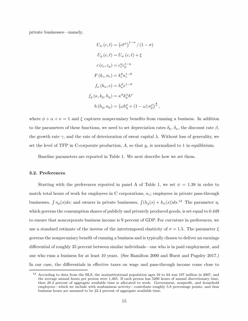
private businesses—namely,

Uw (c, ℓ) =(

cℓψ)1−σ

/ (1− σ)

Up (c, ℓ) = Uw (c, ℓ) + ξ

c (cc, cp) = cηcc1−ηp

F (kc, nc) = kθcn1−θc

fκ (hκ, e) = hϑκe1−ϑ

fy (κ, kp, hy) = κφkαp hν

h (hy, np) =(

ωhρy + (1− ω)nρp)

1

ρ ,

where φ + α + ν = 1 and ξ captures nonpecuniary benefits from running a business. In addition

to the parameters of these functions, we need to set depreciation rates δk, δκ, the discount rate β,

the growth rate γ, and the rate of deterioration of sweat capital λ. Without loss of generality, we

set the level of TFP in C-corporate production, A, so that yc is normalized to 1 in equilibrium.

Baseline parameters are reported in Table 1. We next describe how we set them.

3.2. Preferences

Starting with the preferences reported in panel A of Table 1, we set ψ = 1.38 in order to

match total hours of work for employees in C corporations, nc; employees in private pass-through

businesses,∫

np(s)ds; and owners in private businesses,∫

(hy(s) + hκ(s))ds.12 The parameter η,

which governs the consumption shares of publicly and privately produced goods, is set equal to 0.449

to ensure that noncorporate business income is 9 percent of GDP. For curvature in preferences, we

use a standard estimate of the inverse of the intertemporal elasticity of σ = 1.5. The parameter ξ

governs the nonpecuniary benefit of running a business and is typically chosen to deliver an earnings

differential of roughly 35 percent between similar individuals—one who is in paid employment, and

one who runs a business for at least 10 years. (See Hamilton 2000 and Hurst and Pugsley 2017.)

In our case, the differentials in effective taxes on wage and pass-through income come close to

12 According to data from the BLS, the noninstitutional population ages 16 to 64 was 197 million in 2007, andthe average annual hours per person were 1,465. If each person has 5200 hours of annual discretionary time,then 28.2 percent of aggregate available time is allocated to work. Government, nonprofit, and householdemployees—which we include with nonbusiness activity—contribute roughly 5.8 percentage points, and thusbusiness hours are assumed to be 22.4 percent of aggregate available time.

15

guaranteeing this difference in pre-tax returns to labor, and therefore we set ξ = 0 in our baseline

model and check that variations do not affect our quantitative results. To match a 4 percent annual

interest rate, we set β = 0.98.

3.3. Technologies

Next, consider parameters of technologies reported in panel A of Table 1. For aggregate growth

in technology, γ, we use the U.S. trend rate of 2 percent. The fixed asset shares in C corporations

and private pass-through businesses are set so as to ensure that kc/y and∫

kp(s)ds/y are roughly

2 times GDP and 1 times GDP, respectively, as is the case for the United States.13 This disciplines

our choices for the C-corporate share θ = 0.5 and the private pass-through share α = 0.3. The

capital stocks also depend on our choice of the rate of depreciation. We use NIPA fixed asset

tables, which include both flows and stocks, and set δk = 0.041 to ensure the model values for

investment rates xc/kc and∫

xp(s)/kp(s)ds are consistent.

The private business sector has two production technologies: one for accumulating sweat

capital, fκ, and one for producing goods and services, fy. For fκ, we do not have direct evidence of

the shares and thus use indirect evidence from the BEA’s benchmark 2007 input-output table on

labor and intermediate shares in the advertising and related services sector (NAICS 5418). Based

on these shares, we set ϑ = 0.418. We use the same depreciation rate for fixed assets and sweat

capital because there is no empirical analogue for the latter.14 For fy, we need to estimate share

parameters for sweat capital and labor inputs as well as the elasticity of substitution between

owner and employee time. Since NIPA construction of sweat income includes payments for both

owners’ hours in production hy and accumulated sweat capital, κ, we need additional information

to identify share parameter φ (and, residually, ν).

The additional information that we use to identify the sweat capital share, φ, is Pratt’s Stats’

broker data on sales of private businesses. We use our sample of 6,855 sales over the period 1994–

2017 with records of the purchase-price allocation across different asset categories. Such records

13 These estimates are based on an expanded notion of intellectual property product (IPP) investments, whichare estimated at 12 percent of GDP, rather than those currently counted in NIPA, which are estimated at 4percent of GDP. See Bhandari and McGrattan (2019) for details.

14 In our sensitivity analysis, we check the robustness of this choice as well as our specification for fκ.

16

are kept for tax purposes to determine the purchaser’s basis in each acquired asset and the seller’s

gain or loss on the transfer of each asset. (See IRS Form 8594.) The asset categories include cash

and deposit accounts, government securities, debt instruments, inventory, fixed assets and land,

and intangible assets. The intangibles assets include both goodwill and all Section 197 intangibles,

such as customer bases and trademarks. As we noted earlier, the intangible intensity—or ratio of

the intangible asset value to total asset value—has a mean of 58 percent. We choose φ = 0.15 in

order to generate a comparable average ratio in the model (both here and when we add brokered

sales). In the model, we compute the intangible intensity ii(s) for a business with state s as follows:

ii (s) =vκ (s)

vκ (s) + kp (s), (3.1)

where vκ(s) is the amount of cash needed to leave a business owner indifferent between continuing

in business with sweat capital κ and selling it; that is, vκ(s) satisfies

Vj,p (s) = Vj,w (a+ vκ (s) , 0, ǫ, z) . (3.2)

In effect, vκ(s) is the value of transferable intangible assets.

One potential issue with using the intangible intensity based on broker data is that we may

encounter selection bias, conditioning only on businesses that eventually sold. However, both in

the data and in the model, we find that the intangible intensity is not systematically different when

we condition on different business characteristics. As we document in Bhandari and McGrattan

(2019), the average intangible intensity based on Pratt’s Stats does not vary systematically with

industry or firm size or indicators of distressed sales. Similarly, estimates in the model are not that

different as we vary owner productivities. The reason is that productive owners increase their use

of physical capital as they build their sweat capital in the business, and unproductive owners scale

both down. Later, we formally model selection by extending the theory to allow for the buying

and selling of sweat capital via a competitive broker. Recalibrating the extended model, we find a

similar prediction for the average intangible intensity with φ equal to 15 percent.

Given this value for φ, the share of labor (owner plus employee time) is ν = 0.55, and the

predicted hours of work for business owners,∫

(hy(s)+hκ(s))ds, are roughly 23 percent of all hours

worked in business. This prediction is close to the 25 percent estimate based on data available from

17

the 2007 SBO microsample. The share parameter governing owner and employee hours, ω, is set

equal to 0.425 in order to generate a prediction that 33 percent of aggregate employee compensation

is paid by pass-through businesses, consistent with NIPA. The parameter ρ governs the elasticity

of substitution between owner and employee hours in private business; the more substitutable they

are, the greater the opportunity is for an owner to scale up the business if productivity is high.

We set ρ = 0.5, which implies variation in payroll share per owner hour that is consistent with the

2007 SBO microsample.

Both the income share on sweat capital and the deterioration rate λ of this capital outside

of the business play a quantitatively important role for the age profile of businesses because both

affect the option value for business owners. From the SBO, we have information about the year

business owners started or, in the case of nonfounders, acquired their share of the business. We

use this information to compute a profile of business ages and compare it to model predictions.

The higher the share φ of sweat capital in production (and the lower ν is), the longer the duration

of benefits from sweat in the business. The higher the deterioration rate λ, the more costly it is

to exit and reenter the business sector. This cost naturally lengthens the age of business. Given a

value for φ has been identified using information on intangible intensities of businesses, we set the

deterioration rate λ equal to 0.5 to ensure consistency of the model and data on the age profile.

3.4. Life Cycle

There are several parameters governing life cycle patterns, which are chosen to match overall

U.S. population statistics and those in business. The stochastic aging parameters are set equal to

πy = 0.978 and πo = 0.933 to ensure that one-fourth of the model population is over 65, with the

average duration of working years at 45. We set the old-age productivity shock to ζ = 0.5 and the

sweat deterioration rate at death to λd = 0.9 in order to match business age profiles for young and

old owners. The parameter ι was set to 1, implying that parents are fully altruistic.

3.5. Financing

We have one parameter related to business financing, which is the tightness of the working

capital constraint in (2.6). Based on the work of Hurst and Lusardi (2004) and Chari (2014), we

18

set χ in our baseline model to zero. Using surveys of businesses, Hurst and Lusardi (2004) found

no relationship between wealth and business entry, with the exception of those at the very top

of the wealth distribution. Chari (2014) constructed time series estimates of available funds and

investments using business data from NIPA, Compustat, and the IRS and, found that available

funds for large and small firms were higher than the total invested for virtually every year. Later,

in our sensitivity analysis, we set χ equal to the maximum observed ratio of available funds to

value added found in the samples Chari (2014) considers and show that our results are unchanged.

3.6. Productivity processes

The productivity shocks are modeled as uncorrelated Markov chains with the states and

transition matrices for ǫt and zt shown in Table 1, panel B. The transition matrix for ǫt is consistent

with the estimated wage processes of Low, Meghir, and Pistaferri (2010) for U.S. households in

U.S. Census Survey of Income and Program Participation (SIPP). To construct this matrix, we

take a panel of simulated wages from their estimated quarterly model, annualize the simulated

data, and then run a fixed effect regression of log wages on one lag and a set of controls (namely,

age, age squared, education, and their interactions). We use the estimate of the coefficient on the

log of lagged wages (0.7) and our estimate of the standard deviation of the regression residuals

(0.16) and apply the method of Tauchen (1986) to estimate the Markov chain shown in Table 1,

panel B.

The transition matrix for zt is taken from Debacker, Panousi, and Ramnath (2013), who

use a panel of businesses in the IRS Statistics of Income subsample to construct transitions for

business incomes. We use the same estimates for our productivity transition matrix and find that

the implied transition matrix for business income is not significantly different. For the z grid, we

face the challenge that the upper income bracket in Debacker, Panousi, and Ramnath (2013) is

top-coded to protect privacy. Since we know the income distribution is skewed, we use a squared

log-normal autoregressive process with the variance chosen to generate the 90th percentile business

income relative to the median wage income as in Debacker, Panousi, and Ramnath (2013). We

view our choice of z grid as conservative. Later, in our sensitivity analysis, we introduce a small

number (1 percent) of superstar owners whose incomes are 10 times larger than the median wage

19

earner’s and show that the differences between model predictions with and without sweat activity

are even greater when the skewness of the productivity process is increased.

3.7. Tax Rates

The third set of parameters are the tax rates and schedules reported in panel C of Table

1. We use effective rates based on NIPA government revenues and IRS data. The tax rate on

consumption, τc = 0.065, is found by dividing total sales and excise taxes in NIPA by personal

consumption expenditures. To compute the tax rate on profits, we use information on domestic

earnings from IRS federal and state returns and foreign earnings from the U.S. balance of payments.

The statutory federal tax rate on domestic C-corporate profits is 35 percent, but there is a 9 percent

deduction for firms that qualify for the domestic production deduction. From NIPA data, we know

that 15 percent of corporate tax revenues are paid to the states. Using this information, we compute

a 40 percent tax rate on domestic profits for 2007. To compute an effective rate on all profits,

we use data on global tax rates from KPMG International and BEA balance of payment data on

foreign corporate earnings. In 2007, 27 percent of profits were earned abroad with a weighted

average tax rate of 25 percent. Thus, our estimate for the effective tax rate on profits, τp, is 36

percent.

To construct tax rates on dividends, wages, and sweat income to business owners, we use

data on taxable incomes from the IRS individual income tax returns reported in the Statistics

of Income (SOI) and available by source of income and by size of adjusted gross income (AGI).

Taxable incomes and information on marital status are used to construct weighted federal marginal

tax rates for each AGI income bracket, with weights equal to the fraction of returns filed as married

filing jointly, married filing separately, single, and heads of households. For the federal tax rate on

dividends, we compute an average marginal rate using the same procedure as in Barro and Redlick

(2011). Specifically, if households in AGI income group i pay τi on an additional dollar of income

and earn yi/∑

i yi of the total income, then the average marginal rate is τ =∑

i τiyi/∑

i yi. The

tax rates τi are themselves weighted averages of rates on ordinary, qualified, and untaxed dividends,

with weights equal to the fraction of dividends in each category. We use data for tax year 2007,

which is the same year of the SBO microsample. In that year, owners of taxable accounts also

20

paid roughly 5 percent in state and local taxes on dividend income. Untaxed dividends are held

in pension funds and retirement accounts, which account for 44 percent of all equities owned by

households. Adding federal, state, and local, we estimate a weighted marginal tax rate τd of 13.3

percent.

For the tax schedule Tw(y) of employee labor income in (2.8), we compute the federal marginal

tax rate on an additional dollar of wages and salaries for each AGI income bracket in the SOI. We

add Federal Insurance Contributions Act (FICA) taxes for each bracket; in 2007, those with the

lowest incomes paid 15.3 percent for Social Security and Medicare, while those above the Social

Security cap paid 2.9 percent for Medicare. Additionally, we add a 4 percent tax rate for state

and local taxes. In the model, the income of individual i, yi, is defined as per working-age person,

while the SOI incomes are reported per return. Thus, we divide the SOI incomes per return by the

number of adults per return. The number of adults is proxied by total exemptions less exemptions

for children at home. The result is a nonlinear function that is well approximated by a continuous

piecewise linear curve, with an initial intercept that is set so that aggregate taxes net of transfers

relative to GDP is consistent with U.S. accounts. In the last column of Table 1, panel C, we report

marginal rates Tw ′(y) for tax year 2007. The income levels reported have been normalized by

dividing each by GDP per working-age person. The IRS reports data for 20 AGI brackets, but we

find that the tax function is well approximated by a piecewise function with only seven.

To estimate the tax schedule T b(y) of sweat income to business owners in (2.2), we require tax

audit data in addition to taxable incomes reported in the SOI, since there is significant misreport-

ing on business tax returns. To compute the federal marginal rate for a particular AGI interval, we

estimate the tax paid on reported business income from all sources—namely, sole proprietorships,

partnerships, and S corporations—for an additional dollar of true business income. To do this,

we need estimates from audit data on misreporting for all three business entities. The General

Accounting Office (2009, 2014) reviewed confidential findings from tax audits of S corporations

and estimated that owners report 82 cents per dollar of business net income.15 Johns and Slem-

rod (2010), using data from the National Research Program for tax year 2001, report that sole

proprietors report 43 cents per dollar of income. To infer partners’ misreporting, we use the BEA

15 Note that S corporations also have an incentive to report wage income as a distribution to avoid payroll taxes.See Smith et al. (2017).

21

estimate of total misreporting of unincorporated businesses together with the estimate for sole

proprietors from Johns and Slemrod (2010). With this information, we can infer that partners

would have reported only 47 percent per dollar of income in the 2007 tax year. For the individual

yi values, we follow the same procedure as above and compute a piecewise linear schedule with

per-person estimates normalized by GDP per person. The intercept in the schedule is chosen so

that transfers for the median household are the same regardless of whether they earned business

or wage income.

In panel C of Table 1, we report our estimates. The marginal tax rates for wages and salaries

and business income include federal, state and local, and FICA obligations. What is noteworthy is

how much lower the effective tax rates on owners of private business are than they are on employees

or owners of C corporations, who pay taxes on dividends and corporate profits. On the spending

side, we choose g to ensure that the share of spending on goods and services by the government in

GDP (g/y) is roughly equal to the NIPA value.

3.8. Validation

With the baseline parameters in Table 1, we compute an equilibrium of the model and check

that the implied national accounts and business age profiles are in fact aligned with U.S. data.

Using income and product categories of Section 4.1, Table 2 reports the model and data accounts,

which are, by our choice of parameters, intended to be close.16 Figure 1 shows the age profile

for businesses in the model and data.17 The data are taken from the public-use micro-sample of

the 2007 SBO. We find that 11 percent of owners started running their business in the year of the

survey. For those who started more than four years before, we have only bracketed information and

thus report the averages in the interval. By construction, our model is intended to be consistent

with these data.

Given our model is now parameterized to match key statistics in U.S. data, we next turn to

our main results and policy experiments.

16 Given the number of moments to be matched, we accomplish this with the help of a Nelder-Mead optimizationalgorithm.

17 Here, we display results for all owners but find similar results after conditioning on age, sector, and hours inbusiness.

22

4. Business Valuations

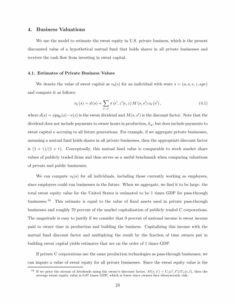
We use the model to estimate the sweat equity in U.S. private business, which is the present

discounted value of a hypothetical mutual fund that holds shares in all private businesses and

receives the cash flow from investing in sweat capital.

4.1. Estimates of Private Business Values

We denote the value of sweat capital as vb(s) for an individual with state s = (a, κ, ǫ, z, age)

and compute it as follows:

vb (s) = d (s) +∑

ǫ′,z′

π (ǫ′, z′|ǫ, z)M (s, s′) vb (s′) , (4.1)

where d(s) = φpyp(s)−e(s) is the sweat dividend andM(s, s′) is the discount factor. Note that the

dividend does not include payments to owner hours in production, hy, but does include payments to

sweat capital κ accruing to all future generations. For example, if we aggregate private businesses,

assuming a mutual fund holds shares in all private businesses, then the appropriate discount factor

is (1 + γ)/(1 + r). Conceptually, this mutual fund value is comparable to stock market share

values of publicly traded firms and thus serves as a useful benchmark when comparing valuations

of private and public businesses.

We can compute vb(s) for all individuals, including those currently working as employees,

since employees could run businesses in the future. When we aggregate, we find it to be large: the

total sweat equity value for the United States is estimated to be 1 times GDP for pass-through

businesses.18 This estimate is equal to the value of fixed assets used in private pass-through

businesses and roughly 70 percent of the market capitalization of publicly traded C corporations.

The magnitude is easy to justify if we consider that 9 percent of national income is sweat income

paid to owner time in production and building the business. Capitalizing this income with the

mutual fund discount factor and multiplying the result by the fraction of time owners put in

building sweat capital yields estimates that are on the order of 1 times GDP.

If private C corporations use the same production technologies as pass-through businesses, we

can impute a value of sweat equity for all private businesses. Since the sweat equity value is the

18 If we price the stream of dividends using the owner’s discount factor, M(s, s′) = Uc(c′, ℓ′)/Uc(c, ℓ), then theaverage sweat equity value is 0.87 times GDP, which is lower since owners face idiosyncratic risk.

23

present value of pre-tax cash flow to a hypothetical mutual fund, we simply take the result for

pass-through businesses (1 GDP) and multiply by the ratio of post-audit incomes of all private

businesses relative to pass-through businesses. Bhandari et al. (2019) estimate this ratio to be

1.2 using IRS data from corporate filings of Schedule M-3 and BEA imputations of misreported

corporate incomes. The Schedule M-3 links IRS data with the Securities and Exchange Commission

10-K filings for publicly-traded firms, allowing researchers to infer the split of income earned by

privately and publicly held C corporations. For 2007, the implied income for privately held C

corporations was 1.8 percent of GDP, which, if added to the 9 percent of pass-through income,

yields a ratio of private to pass-through net income of 1.2. This, in turn, implies a private business

sweat equity value of 1.2 times GDP, which is roughly 84 percent of the market capitalization of

publicly traded C corporations.

The incomes being valued in (4.1) are payments to both nontransferable productivity z, which

is specific to an owner, and transferable sweat capital κ, which is eventually bequeathed or sold.

Thus, the mutual fund shares would be worth more than the cash value vκ in (3.2) given the latter

is the price offered current owners only for their sweat capital. For our baseline parameterization

(using data for pass-through businesses only), the average value for vb(s), if we condition on

business owners, is 1.24 times GDP per capita, whereas the average value for vκ(s) is 0.37 times

GDP per capita, or 30 percent of the sweat equity value. A value of 0.37 implies a price of goodwill

that is roughly equivalent to 2 times annual business income—a finding that is consistent with the

Pratt’s Stats data where we find this ratio to be about 1.5 for sole proprietors and between 2 and

3 for partnerships and S corporations.

In Table 3, we report average valuations along with cross-sectional information on valuations,

intangible intensities, and business returns for the model calibrated to pass-through data. In the

first two columns, we report the cross-sectional statistics for the sweat capital sale values, vκ(s),

and the associated intangible intensities, ii(s), defined in (3.1). The sale values are increasing

and convex in the level of sweat capital, κ. The intuition for this pattern comes from the feature

that owner time is finite and disutility of hours is convex. Therefore, accumulating higher and

higher stocks is very costly, given that it takes many years and some luck to build a business, but

owners are compensated for their time when they sell the business. Since we computed vκ(s) for

24

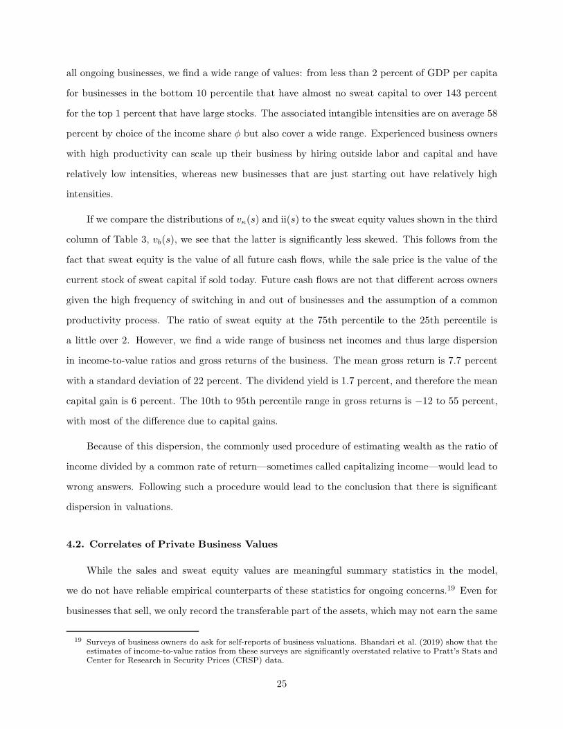
all ongoing businesses, we find a wide range of values: from less than 2 percent of GDP per capita

for businesses in the bottom 10 percentile that have almost no sweat capital to over 143 percent

for the top 1 percent that have large stocks. The associated intangible intensities are on average 58

percent by choice of the income share φ but also cover a wide range. Experienced business owners

with high productivity can scale up their business by hiring outside labor and capital and have

relatively low intensities, whereas new businesses that are just starting out have relatively high

intensities.

If we compare the distributions of vκ(s) and ii(s) to the sweat equity values shown in the third

column of Table 3, vb(s), we see that the latter is significantly less skewed. This follows from the

fact that sweat equity is the value of all future cash flows, while the sale price is the value of the

current stock of sweat capital if sold today. Future cash flows are not that different across owners

given the high frequency of switching in and out of businesses and the assumption of a common

productivity process. The ratio of sweat equity at the 75th percentile to the 25th percentile is

a little over 2. However, we find a wide range of business net incomes and thus large dispersion

in income-to-value ratios and gross returns of the business. The mean gross return is 7.7 percent

with a standard deviation of 22 percent. The dividend yield is 1.7 percent, and therefore the mean

capital gain is 6 percent. The 10th to 95th percentile range in gross returns is −12 to 55 percent,

with most of the difference due to capital gains.

Because of this dispersion, the commonly used procedure of estimating wealth as the ratio of

income divided by a common rate of return—sometimes called capitalizing income—would lead to

wrong answers. Following such a procedure would lead to the conclusion that there is significant

dispersion in valuations.

4.2. Correlates of Private Business Values

While the sales and sweat equity values are meaningful summary statistics in the model,

we do not have reliable empirical counterparts of these statistics for ongoing concerns.19 Even for

businesses that sell, we only record the transferable part of the assets, which may not earn the same

19 Surveys of business owners do ask for self-reports of business valuations. Bhandari et al. (2019) show that theestimates of income-to-value ratios from these surveys are significantly overstated relative to Pratt’s Stats andCenter for Research in Security Prices (CRSP) data.

25

future dividends as it would with the former owner. Here, we report statistics for variables that

are empirically measurable and potentially correlated with sweat capital and the corresponding

business valuations. In doing so, we illustrate how researchers using standard measures of firm

markups and TFP can be mislead if they ignore intangible investments made by firms.

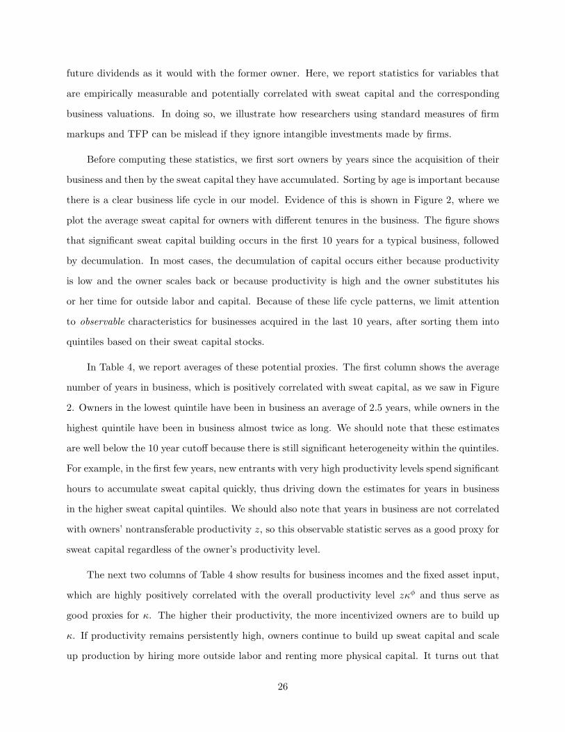
Before computing these statistics, we first sort owners by years since the acquisition of their

business and then by the sweat capital they have accumulated. Sorting by age is important because

there is a clear business life cycle in our model. Evidence of this is shown in Figure 2, where we

plot the average sweat capital for owners with different tenures in the business. The figure shows

that significant sweat capital building occurs in the first 10 years for a typical business, followed

by decumulation. In most cases, the decumulation of capital occurs either because productivity

is low and the owner scales back or because productivity is high and the owner substitutes his

or her time for outside labor and capital. Because of these life cycle patterns, we limit attention

to observable characteristics for businesses acquired in the last 10 years, after sorting them into

quintiles based on their sweat capital stocks.

In Table 4, we report averages of these potential proxies. The first column shows the average

number of years in business, which is positively correlated with sweat capital, as we saw in Figure

2. Owners in the lowest quintile have been in business an average of 2.5 years, while owners in the

highest quintile have been in business almost twice as long. We should note that these estimates

are well below the 10 year cutoff because there is still significant heterogeneity within the quintiles.

For example, in the first few years, new entrants with very high productivity levels spend significant

hours to accumulate sweat capital quickly, thus driving down the estimates for years in business

in the higher sweat capital quintiles. We should also note that years in business are not correlated

with owners’ nontransferable productivity z, so this observable statistic serves as a good proxy for

sweat capital regardless of the owner’s productivity level.

The next two columns of Table 4 show results for business incomes and the fixed asset input,

which are highly positively correlated with the overall productivity level zκφ and thus serve as

good proxies for κ. The higher their productivity, the more incentivized owners are to build up

κ. If productivity remains persistently high, owners continue to build up sweat capital and scale

up production by hiring more outside labor and renting more physical capital. It turns out that

26

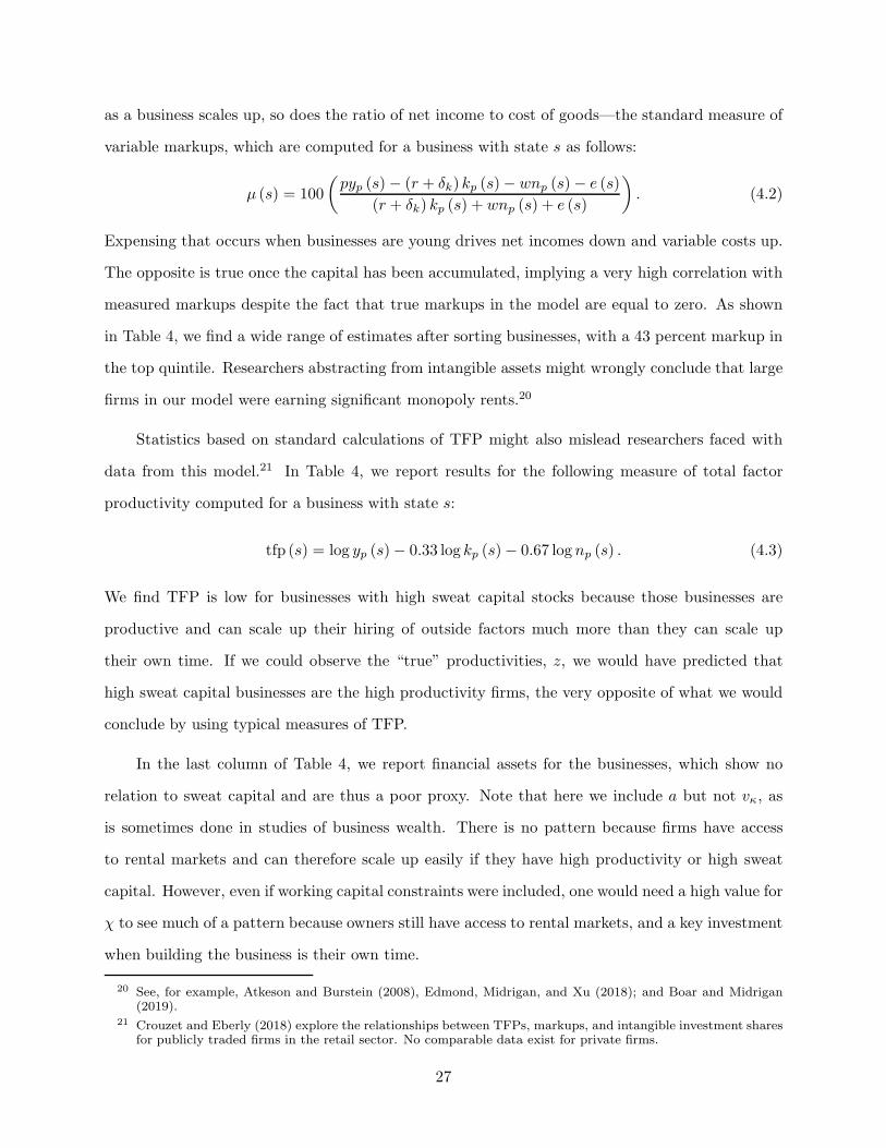
as a business scales up, so does the ratio of net income to cost of goods—the standard measure of

variable markups, which are computed for a business with state s as follows:

µ (s) = 100

(

pyp (s)− (r + δk) kp (s)− wnp (s)− e (s)

(r + δk) kp (s) + wnp (s) + e (s)

)

. (4.2)

Expensing that occurs when businesses are young drives net incomes down and variable costs up.

The opposite is true once the capital has been accumulated, implying a very high correlation with

measured markups despite the fact that true markups in the model are equal to zero. As shown

in Table 4, we find a wide range of estimates after sorting businesses, with a 43 percent markup in

the top quintile. Researchers abstracting from intangible assets might wrongly conclude that large

firms in our model were earning significant monopoly rents.20

Statistics based on standard calculations of TFP might also mislead researchers faced with

data from this model.21 In Table 4, we report results for the following measure of total factor

productivity computed for a business with state s:

tfp (s) = log yp (s)− 0.33 log kp (s)− 0.67 lognp (s) . (4.3)

We find TFP is low for businesses with high sweat capital stocks because those businesses are

productive and can scale up their hiring of outside factors much more than they can scale up

their own time. If we could observe the “true” productivities, z, we would have predicted that

high sweat capital businesses are the high productivity firms, the very opposite of what we would

conclude by using typical measures of TFP.

In the last column of Table 4, we report financial assets for the businesses, which show no

relation to sweat capital and are thus a poor proxy. Note that here we include a but not vκ, as

is sometimes done in studies of business wealth. There is no pattern because firms have access

to rental markets and can therefore scale up easily if they have high productivity or high sweat

capital. However, even if working capital constraints were included, one would need a high value for

χ to see much of a pattern because owners still have access to rental markets, and a key investment

when building the business is their own time.

20 See, for example, Atkeson and Burstein (2008), Edmond, Midrigan, and Xu (2018); and Boar and Midrigan(2019).

21 Crouzet and Eberly (2018) explore the relationships between TFPs, markups, and intangible investment sharesfor publicly traded firms in the retail sector. No comparable data exist for private firms.

27

In summary, we find large sweat equity values for private businesses and significant dispersion

in business intangible intensities and returns. Roughly 30 percent of the value is attributable to

transferable sweat capital, and 70 percent of the value is due to nontransferable owner-specific

productivity. High-value businesses are older, larger in scale, and appear to have high measured

markups.

Next, we consider the tax experiments and show that sweat capital and owner time in pro-

duction play an important role for our quantitative results.

5. Tax Policy Experiments

To quantify the role of owner time in the business when evaluating tax changes, we make two

types of comparisons. First, we contrast the effect of lowering tax rates on private pass-through

businesses and C corporations in our baseline model with the effect of lowering them in a nested

model that has owner time fixed.22 Second, we contrast the impact of lowering tax rates on labor

income earned by owners and by employees.

For comparability across experiments, we lower average marginal tax rates (AMTR) by the

same amount:

∆ log (1− τAMTR) = 0.156,

which is on the order of the tax change for corporations in the 2017 U.S. tax reform. The AMTR

for private business and wages is computed by taking a weighted average of each filer’s marginal

rate, with weights given by the taxable net income as in Barro and Redlick (2011). In the case

of private business, lowering all marginal rates by 50.6 percent implies a 15.6 percentage point

decline in the AMTR. For wage earners, we lower marginal rates by 25.5 percent to achieve the

same result. In both cases, we adjust intercepts in the piecewise linear tax schedules to ensure the

schedule remains continuous. For C corporations, there is only one rate, so the AMTR is simply

the income tax rate τp, which is lowered from 36 percent to 26 percent for federal- and state-level

22 The policy experiments we conduct are not intended to be a careful study of a particular reform in U.S. historybut are instead a proof of concept intended to highlight the economic forces at work in our model with sweatactivity. For related work that focuses specifically on the recent Tax Cuts and Jobs Act of 2017, see Barro andFurman (2018).

28

taxes. In each case, we compute the stationary equilibrium associated with the new taxes. Debt

levels adjust so that the government budget constraint is satisfied.

5.1. Lower Taxes on Business

We start by comparing aggregate results in the baseline model to those of the nested model

that abstracts from owner time in production and building sweat capital. The latter is the standard

framework used in the study of entrepreneurial choice, which, as mentioned earlier, is a version

of the Lucas (1978) span-of-control model. There are two main takeaways from this exercise.

First, the response to lowering private business tax rates is much larger in the baseline model

than in Lucas (1978)—both on the intensive and extensive margins—with most of the change due

to highly productive owners and not necessarily those with the highest financial assets or sweat

capital. Second, lowering the corporate income tax rate has similar effects for most aggregate

variables, with the exception of hours.

5.1.1. Aggregate Responses

Consider first a lowering of just the private business tax rates. In the first two columns of

Table 5, the main results for this experiment are shown for the baseline model with sweat capital

and hours and the nested Lucas (1978) model that has a production function given by

yp = zkαp nνp. (5.1)

In this nested case, we set φ = ω = 0, and we reparameterize the consumption share η and labor

share ν in order to match two statistics: the share of employee hours allocated to private business

and the share of pass-through income in total income. The new values are η = 0.50 and ν = 0.39.

Our first observation is that with a lowering of tax rates, the change in total private sector

output is predicted to be quite small in the Lucas (1978) model without sweat activity. In fact,

output falls by 0.4 percentage points, whereas output in the private sector rises by 1.9 percentage

points in the baseline model with sweat activity. To understand these differences, consider first

the decisions of very productive owners. These owners are not marginal in terms of their entry

or exit decisions irrespective of the tax rates. These owners in the Lucas (1978) environment will

expense all the variable factors, and therefore the only taxed factor is the fixed managerial input.

29

In this case, if we ignore the general equilibrium effects on prices and wages, the model predicts

no change in response to a lowering of tax rates for very productive firms.23 On the other hand, in

the baseline model, we predict a quantitatively large response to the lower income tax rates on the

intensive margin. As we show in Table 5, owners increase time in production by 17.5 percent and

time in building their business by 8.6 percent. As a result, output in the private business sector is

higher by 1.9 percent, and sweat capital is higher by 4 percent.

In both models, lowering tax rates on business income leads to more entry. In the Lucas

(1978) model, the main driver for the size of the extensive margin response is the mass of agents

at the exogenous productivity entry threshold. In contrast, when we model sweat activity, the

extensive margin changes are more substantial. Post-entry owners work harder, resulting in a

larger endogenous productivity zκφ, which amplifies the incentives to enter. In the baseline model,

the fraction of owners increases by 7.9 percent and in the no-sweat Lucas (1978) model, the fraction

of owners increases by only 3.5 percent.

The large increase in owners’ hours is accompanied by a large decrease of 5.8 percent in

private business employee hours for the baseline model—much larger than the 1.4 percent decline

in the no-sweat model. We find that fixed asset investments also decline in both models but only

modestly.

When we compare aggregate statistics for this tax experiment for the models with and without

sweat activity, we find stark differences in measured total factor productivity, measured markups,

and total hours. For example, if we compare aggregate TFP in the private sector as it is typically

measured—the logarithm of∫

yp(s)ds divided by∫

kp(s).33np(s)

.67ds—we find an increase of 6.3

percent in the baseline model but only 0.8 percent in the no-sweat model. This difference arises

because measured TFP picks up changes in the unmeasured factors of production. If we compare

the aggregate markup in the private sector as it is typically measured—total business net income

divided by total variable costs for capital, labor, and expenses—we find a large increase of 7

percent in the baseline and no change in the no-sweat model. In fact, true markups are zero in

both regardless of tax policy. Predictions for aggregate hours are also different, since owner time

23 To see this formally, consider a simpler case where the tax rate on business is linear and firms maximize:(1 − τb)(pyp − wnp − (r + δk)kp). In this case, the first-order conditions with respect to labor np and fixed

assets kp are independent of τb.

30

is fixed in the no-sweat model. We find an increase of 1.5 percent in the baseline and a decline of

1.4 percent in the no-sweat model. The other aggregate comparisons for C corporations and the

overall economy are similar in the two models given the only modification we made was to private

business production in (5.1). For example, the differences for aggregate GDP and consumption are

on the order of 0.1 percentage points.

In the right panel of Table 5, we show the results for lowering marginal rates on private business

net incomes as before and additionally lowering the corporate profits tax rate τp comparably by

15.6 percentage points. Lower profits taxes have a significant effect on fixed asset investments, with

changes that are roughly the same in the two models. As we show in Table 5, both models predict

a fixed asset investment increase of roughly 7.5 percent in private businesses and 23 percent in C

corporations. As before, we find similar results for the aggregate data. For example, in both models,

wages rise by close to 10 percent, fixed assets rise by 17.5 percent, and GDP and consumption are

higher by a little more than 7 percent. The main exceptions are private sector outcomes such as

the measured TFP and markup as well as total hours, all of which rise significantly in the model

with sweat but not in the one without.

5.1.2. Distributional Responses

To better highlight the mechanisms at work in the baseline model with sweat activity, we next

explore the distributional impacts of lowering just the tax on private business, T b. We first sort

businesses into bins using three different sorts: first by their productivity z, second by sweat capital

stocks κ, and third by financial asset balances a. We then attribute the total change in a particular

variable of interest to the different bins, with contributions summing to the total change. The point

of the computation is to show that the method of sorting affects the results: high z businesses are

not the same as high κ businesses or high a businesses.

In Table 6, we report the results of the decomposition for changes in sweat capital, κ, owner

hours, hy + hκ, and employee hours, np, arising from a change in lower tax rates on private

business. Since z takes on five values, we sort businesses using the discrete values. Since κ

and a are continuous, we assign owners to quintiles. Sorting by productivity, we find that the

highest productivity (z) businesses contribute the most to the total changes in the private business

31

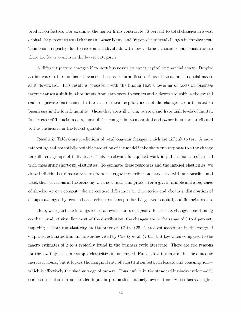
production factors. For example, the high-z firms contribute 56 percent to total changes in sweat

capital, 92 percent to total changes in owner hours, and 98 percent to total changes in employment.

This result is partly due to selection: individuals with low z do not choose to run businesses so

there are fewer owners in the lowest categories.

A different picture emerges if we sort businesses by sweat capital or financial assets. Despite

an increase in the number of owners, the post-reform distributions of sweat and financial assets

shift downward. This result is consistent with the finding that a lowering of taxes on business

income causes a shift in labor inputs from employees to owners and a downward shift in the overall

scale of private businesses. In the case of sweat capital, most of the changes are attributed to

businesses in the fourth quintile—those that are still trying to grow and have high levels of capital.

In the case of financial assets, most of the changes in sweat capital and owner hours are attributed

to the businesses in the lowest quintile.

Results in Table 6 are predictions of total long-run changes, which are difficult to test. A more

interesting and potentially testable prediction of the model is the short-run response to a tax change

for different groups of individuals. This is relevant for applied work in public finance concerned

with measuring short-run elasticities. To estimate these responses and the implied elasticities, we

draw individuals (of measure zero) from the ergodic distribution associated with our baseline and

track their decisions in the economy with new taxes and prices. For a given variable and a sequence

of shocks, we can compute the percentage differences in time series and obtain a distribution of

changes averaged by owner characteristics such as productivity, sweat capital, and financial assets.

Here, we report the findings for total owner hours one year after the tax change, conditioning

on their productivity. For most of the distribution, the changes are in the range of 3 to 4 percent,

implying a short-run elasticity on the order of 0.2 to 0.25. These estimates are in the range of

empirical estimates from micro studies cited by Chetty et al. (2011) but low when compared to the

macro estimates of 2 to 3 typically found in the business cycle literature. There are two reasons

for the low implied labor supply elasticities in our model. First, a low tax rate on business income

increases hours, but it lowers the marginal rate of substitution between leisure and consumption—

which is effectively the shadow wage of owners. Thus, unlike in the standard business cycle model,

our model features a non-traded input in production—namely, owner time, which faces a higher

32

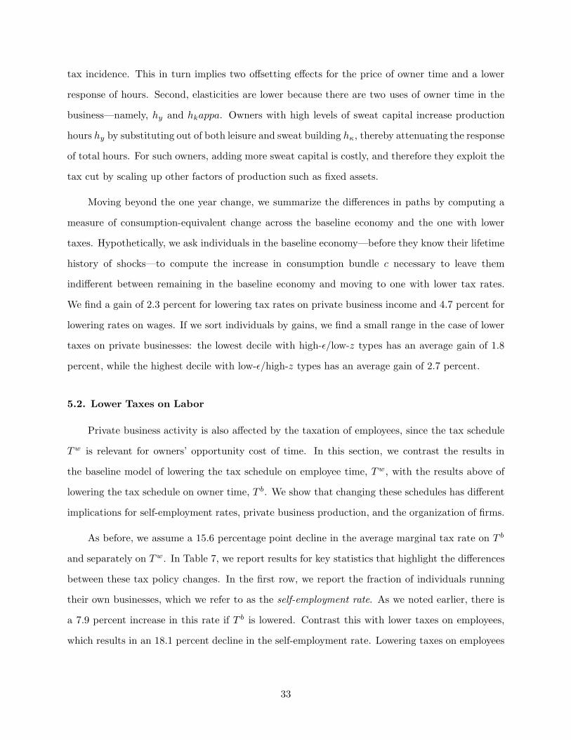
tax incidence. This in turn implies two offsetting effects for the price of owner time and a lower

response of hours. Second, elasticities are lower because there are two uses of owner time in the

business—namely, hy and hkappa. Owners with high levels of sweat capital increase production

hours hy by substituting out of both leisure and sweat building hκ, thereby attenuating the response

of total hours. For such owners, adding more sweat capital is costly, and therefore they exploit the

tax cut by scaling up other factors of production such as fixed assets.

Moving beyond the one year change, we summarize the differences in paths by computing a

measure of consumption-equivalent change across the baseline economy and the one with lower

taxes. Hypothetically, we ask individuals in the baseline economy—before they know their lifetime

history of shocks—to compute the increase in consumption bundle c necessary to leave them

indifferent between remaining in the baseline economy and moving to one with lower tax rates.

We find a gain of 2.3 percent for lowering tax rates on private business income and 4.7 percent for

lowering rates on wages. If we sort individuals by gains, we find a small range in the case of lower

taxes on private businesses: the lowest decile with high-ǫ/low-z types has an average gain of 1.8

percent, while the highest decile with low-ǫ/high-z types has an average gain of 2.7 percent.

5.2. Lower Taxes on Labor

Private business activity is also affected by the taxation of employees, since the tax schedule

Tw is relevant for owners’ opportunity cost of time. In this section, we contrast the results in

the baseline model of lowering the tax schedule on employee time, Tw, with the results above of

lowering the tax schedule on owner time, T b. We show that changing these schedules has different

implications for self-employment rates, private business production, and the organization of firms.

As before, we assume a 15.6 percentage point decline in the average marginal tax rate on T b

and separately on Tw. In Table 7, we report results for key statistics that highlight the differences

between these tax policy changes. In the first row, we report the fraction of individuals running

their own businesses, which we refer to as the self-employment rate. As we noted earlier, there is

a 7.9 percent increase in this rate if T b is lowered. Contrast this with lower taxes on employees,

which results in an 18.1 percent decline in the self-employment rate. Lowering taxes on employees

33

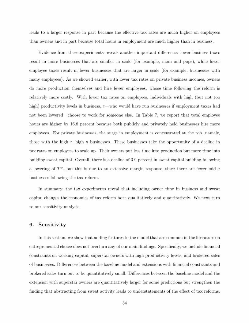
leads to a larger response in part because the effective tax rates are much higher on employees

than owners and in part because total hours in employment are much higher than in business.

Evidence from these experiments reveals another important difference: lower business taxes

result in more businesses that are smaller in scale (for example, mom and pops), while lower

employee taxes result in fewer businesses that are larger in scale (for example, businesses with

many employees). As we showed earlier, with lower tax rates on private business incomes, owners

do more production themselves and hire fewer employees, whose time following the reform is

relatively more costly. With lower tax rates on employees, individuals with high (but not too

high) productivity levels in business, z—who would have run businesses if employment taxes had

not been lowered—choose to work for someone else. In Table 7, we report that total employee

hours are higher by 16.8 percent because both publicly and privately held businesses hire more

employees. For private businesses, the surge in employment is concentrated at the top, namely,

those with the high z, high κ businesses. These businesses take the opportunity of a decline in

tax rates on employees to scale up. Their owners put less time into production but more time into

building sweat capital. Overall, there is a decline of 3.9 percent in sweat capital building following

a lowering of Tw, but this is due to an extensive margin response, since there are fewer mid-κ

businesses following the tax reform.

In summary, the tax experiments reveal that including owner time in business and sweat

capital changes the economics of tax reform both qualitatively and quantitatively. We next turn

to our sensitivity analysis.

6. Sensitivity

In this section, we show that adding features to the model that are common in the literature on

entrepreneurial choice does not overturn any of our main findings. Specifically, we include financial

constraints on working capital, superstar owners with high productivity levels, and brokered sales

of businesses. Differences between the baseline model and extensions with financial constraints and

brokered sales turn out to be quantitatively small. Differences between the baseline model and the

extension with superstar owners are quantitatively larger for some predictions but strengthen the

finding that abstracting from sweat activity leads to understatements of the effect of tax reforms.

34

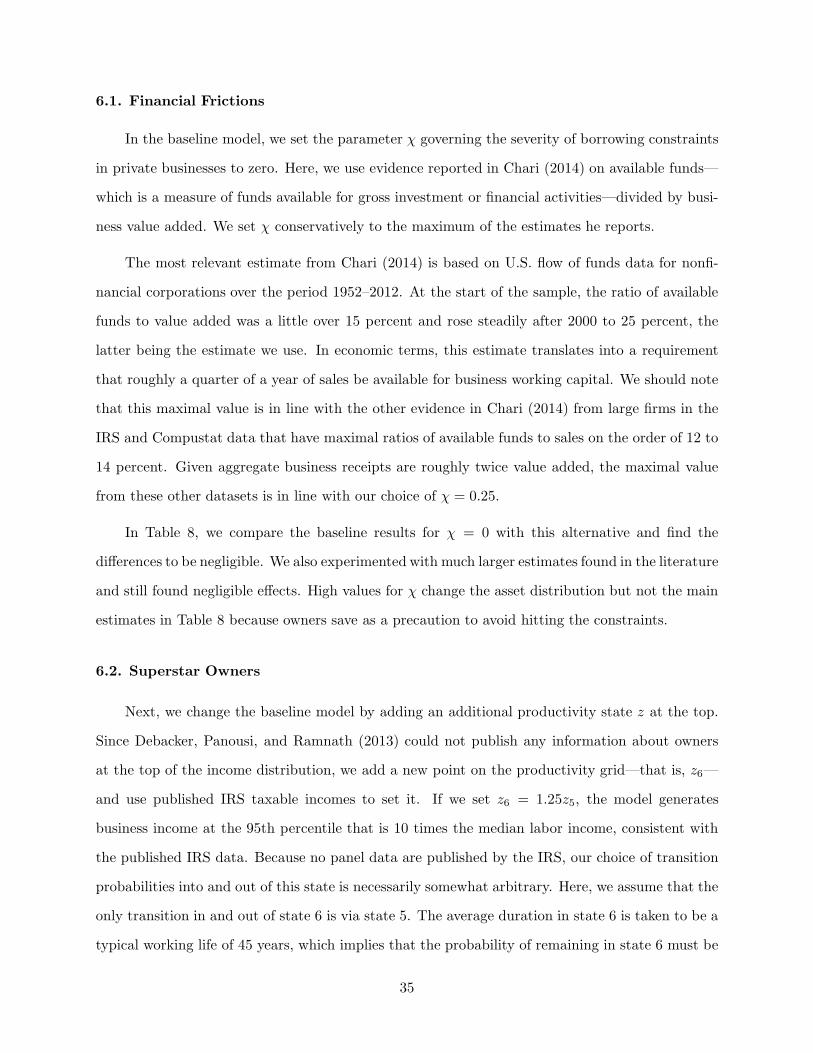
6.1. Financial Frictions

In the baseline model, we set the parameter χ governing the severity of borrowing constraints

in private businesses to zero. Here, we use evidence reported in Chari (2014) on available funds—

which is a measure of funds available for gross investment or financial activities—divided by busi-

ness value added. We set χ conservatively to the maximum of the estimates he reports.

The most relevant estimate from Chari (2014) is based on U.S. flow of funds data for nonfi-

nancial corporations over the period 1952–2012. At the start of the sample, the ratio of available

funds to value added was a little over 15 percent and rose steadily after 2000 to 25 percent, the

latter being the estimate we use. In economic terms, this estimate translates into a requirement

that roughly a quarter of a year of sales be available for business working capital. We should note

that this maximal value is in line with the other evidence in Chari (2014) from large firms in the

IRS and Compustat data that have maximal ratios of available funds to sales on the order of 12 to

14 percent. Given aggregate business receipts are roughly twice value added, the maximal value

from these other datasets is in line with our choice of χ = 0.25.

In Table 8, we compare the baseline results for χ = 0 with this alternative and find the

differences to be negligible. We also experimented with much larger estimates found in the literature

and still found negligible effects. High values for χ change the asset distribution but not the main

estimates in Table 8 because owners save as a precaution to avoid hitting the constraints.

6.2. Superstar Owners

Next, we change the baseline model by adding an additional productivity state z at the top.

Since Debacker, Panousi, and Ramnath (2013) could not publish any information about owners

at the top of the income distribution, we add a new point on the productivity grid—that is, z6—

and use published IRS taxable incomes to set it. If we set z6 = 1.25z5, the model generates

business income at the 95th percentile that is 10 times the median labor income, consistent with

the published IRS data. Because no panel data are published by the IRS, our choice of transition

probabilities into and out of this state is necessarily somewhat arbitrary. Here, we assume that the

only transition in and out of state 6 is via state 5. The average duration in state 6 is taken to be a

typical working life of 45 years, which implies that the probability of remaining in state 6 must be

35

equal to 1− 1/45. We assume that the probability of transitioning from state 5 to state 6 is equal

to the probability of transitioning from state 6 to 5 and choose it in such a way so as to ensure that

only 1 percent of owners are in the high productivity state in the stationary distribution. We also

recalibrate the deterioration rate λ to 0.7 to generate a consistent acquisition profile as in Figure

1.

We should note this version of the model passes a standard litmus test for researchers studying

income and wealth dispersion—namely, that wealth is more dispersed than income. (See Castaneda,

Diaz-Giminez, and Rios-Rull, 2003.) Furthermore, Quadrini (2000) reports evidence that wealth-

to-income ratios are significantly higher for business owners than for workers. Our model predicts

both greater dispersion in wealth than in income and higher wealth-to-income ratios for business

owners relative to workers. If we drop individuals in the top and bottom income deciles—those

with negative incomes or large inheritances—we find wealth-to-income ratios in the range of 1 to

5.7 for workers and 3.5 to 22.7 for business owners.24

In Table 8, we report our main statistics for this case. With higher variability in the produc-

tivity process, we find a higher sweat equity value of 1.15 times GDP for mutual fund investors and

a higher average gross return of 10.4 percent. The intangible intensity is 56 percent and thus not

much different from the baseline. In terms of tax experiments, we find larger average responses.

Looking across the distribution of owners, we find that the highest-z superstar owners account for

a very small portion of the total change.

6.3. Brokered Sales

The final extension that we consider is to explicitly introduce brokered sales into the baseline

model. In this section, we describe the problem of a broker who buys and sells sweat capital and

the data used to discipline additional parameters. Because few U.S. businesses sell in any given

year, we find that the extended model predictions are close to those of our baseline model without

brokered sales.

With sales, individuals choose whether to buy or sell κ simultaneously with occupation. That

24 We do not attempt to match these statistics to survey data used by the previous literature because of docu-mented measurement issues with business wealth statistics elsewhere. See Bhandari et al. (2019).

36

is, given their state s and age (y or o), all individuals can decide whether to sell their sweat capital

κ and become a worker, keep the κ and become a worker, run a business with the κ they currently

have, or run a business after buying additional κ from the broker. If individuals are indifferent

between selling and not selling, we break the tie with probability πf . Sellers exchange κ for cash

in the amount vκ(s), which would be the value of the κ after paying any capital gains tax. Brokers

own a technology to produce new businesses of size κ. They offer homogeneous price-quantity

bundles (pκ, κ) to all potential buyers. There is free entry in the broker market, and the zero profit

condition for the broker is

pκ

∫

1buy (s) f (s) ds = πf∫

vκ (s)1sell (s) f (s) ds,

where f(s) is the measure of type s individuals. Our definition of a competitive equilibrium must

be amended to include (vκ(s), pκ) and the condition that the sale price is such that sellers are

indifferent between continuing to run their businesses and entering employment with additional

cash, as in (3.2). Any capital gains taxation would also be included in (2.15).

To discipline πf and κ, we use microdata from the 2007 SBO microsample. The parameter

πf is set such that the fraction of exiting owners who sold their businesses is roughly 9 percent.

The size κ is set such that we match the fact that 8 percent of SBO businesses with at least one

owner reported that they acquired their share of the business over the period 2000–2007 through

a purchase. We also recalibrate the deterioration rate λ to 0.7 and ω to 0.478 in order to match

the acquisition profile and sweat income share.

Results are reported in Table 5 and show that the main results are robust to including bro-

kered sales. Specifically, we continue to find high estimates for sweat equity values and intangible

intensities and our predictions for the tax experiments are close to our baseline model. The main

reason we find little change is the small number of sales that occur in the data. Given that we

parameterize the model to match this fact, we find little change in the main results.

7. Conclusions

In this paper, we developed a theory of intangible investments made by private business owners

and used it to reassess central questions in public finance. We found that abstracting from these

37

investments has quantitatively important consequences for both measurement and policy. We find

that the stocks of intangible assets are as large as those of tangible assets. We find that leaving

them out of tax analyses leads to significant understatements of the impact of lowering tax rates

on private businesses. We view these findings as a proof of concept for future analyses of specific

tax reforms.

There are several extensions of our model that should be explored if better data become

available. We model individuals choosing between paid and self-employment when in fact there are

those that engage in both activities or have family members that do so. In our model, sweat capital

cannot be accumulated while in paid employment or by employees, which may have consequences

for measuring the stock. The choice of legal form of organization is not included here, but would

likely depend on expectations about current and future tax policies. Especially relevant is the

choice of becoming a private C corporation that pays corporate income taxes but has few owners

with significant exposure to idiosyncratic risk. Finally, more can be done in modeling business

sales, especially with regards to the bargaining of the purchase price.

38

References

Aiyagari, S. Rao. 1994. “Uninsured Idiosyncratic Risk and Aggregate Saving.” Quarterly Journal

of Economics 109(3): 659–684.

Angeletos, George-Marios and Laurent-Emmanuel Calvet. 2006. “Idiosyncratic Production Risk,Growth and the Business Cycle.” Journal of Monetary Economics 53(6): 1095–1115.

Arkolakis, Costas. 2010. “Market Penetration Costs and the New Consumers Margin in Interna-tional Trade.” Journal of Political Economy 118(6): 1151–1199.

Atkeson, Andrew and Patrick J. Kehoe. 2005. “Modeling and Measuring Organizational Capital.”Journal of Political Economy 113(6): 1026–1053.

Atkeson, Andrew and Ariel Burstein. 2008. “Pricing-to-Market, Trade Costs, and InternationalRelative Prices.” American Economic Review 98(5): 1998–2031.

Barro, Robert J. and Jason Furman. 2018. “The Macroeconomic Effects of the 2017 Tax Reform.”Brookings Papers on Economic Activity Spring.

Barro, Robert J. and Charles J. Redlick. 2011. “Macroeconomic Effects from Government Pur-chases and Taxes.” The Quarterly Journal of Economics 126(1): 51–102.

Belo, Frederico, Xiaoji Lin, and Maria Ana Vitorino. 2014. “Brand Capital and Firm Value.”Review of Economic Dynamics 17(1): 150–169.

Ben-Porath, Yoram. 1967. “The Production of Human Capital and the Life Cycle of Earnings.”Journal of Political Economy 75(4): 352–365.

Bhandari, Anmol, Serdar Birinci, Ellen R. McGrattan, and Kurt See. 2019. “What Do SurveyData Tell Us about U.S. Businesses?” American Economic Review: Insights, forthcoming.

Bhandari, Anmol and Ellen R. McGrattan. 2019. “Data Appendix: Sweat Equity in U.S. PrivateBusiness.” Working paper, University of Minnesota.

Blanchard, Olivier J. 1985. “Debt, Deficits, and Finite Horizons.” Journal of Political Economy

93(2), 223–247.

Boar, Corina and Virgiliu Midrigan. 2019. “Markups and Inequality.” NBER Working Paper25952.

Buera, Francisco J. 2009. “A Dynamic Model of Entrepreneurship with Borrowing Constraints:Theory and Evidence” Annals of Finance 5(3): 443–464.

Buera, Francisco J. and Yongseok Shin. 2013. “Financial Frictions and the Persistence of History:A Quantitative Exploration.” Journal of Political Economy 121(2): 221–272.

Cagetti, Marco and Mariacristina De Nardi. 2006. “Entrepreneurship, Frictions, and Wealth.”Journal of Political Economy 114(5): 835–870.

Castaneda, Ana, Javier Diaz-Gimenez, Jose Victor Rios-Rull. 2003. “Accounting for the U.S.Earnings and Wealth Inequality.” Journal of Political Economy 111(4): 818–857.

Cole, Rebel A. and Tatyana Sokolyk. 2018. “How Do Firms Choose Legal Form of Organization?”Working paper, Florida Atlantic University.

Chari, V.V. 2014. “A Macroeconomist’s Wish List for Financial Data.” in Risk Topology: Systemic

Risk and Macro Modeling, eds. M. Brunnemeier and A. Krishnamurthy, 215–232. Chicago:University of Chicago Press.

39

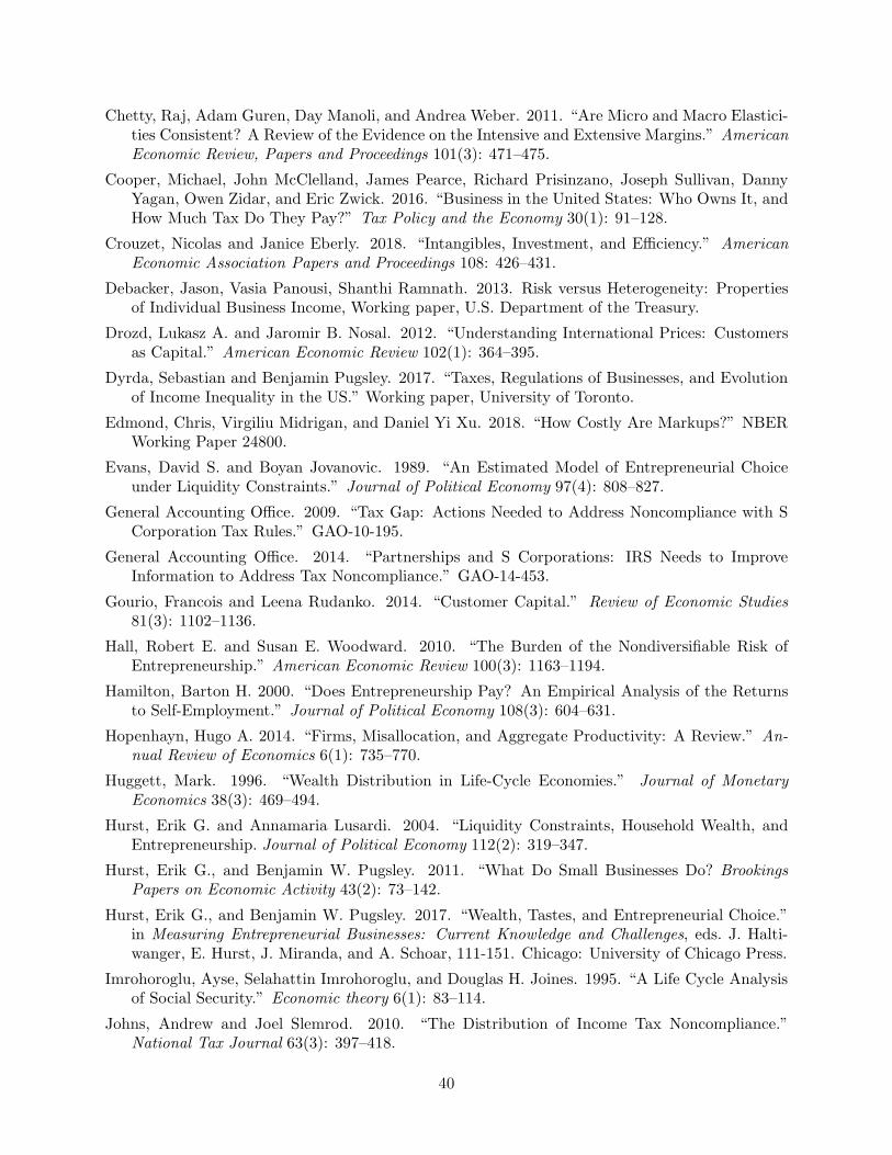
Chetty, Raj, Adam Guren, Day Manoli, and Andrea Weber. 2011. “Are Micro and Macro Elastici-ties Consistent? A Review of the Evidence on the Intensive and Extensive Margins.” American

Economic Review, Papers and Proceedings 101(3): 471–475.

Cooper, Michael, John McClelland, James Pearce, Richard Prisinzano, Joseph Sullivan, DannyYagan, Owen Zidar, and Eric Zwick. 2016. “Business in the United States: Who Owns It, andHow Much Tax Do They Pay?” Tax Policy and the Economy 30(1): 91–128.

Crouzet, Nicolas and Janice Eberly. 2018. “Intangibles, Investment, and Efficiency.” American

Economic Association Papers and Proceedings 108: 426–431.

Debacker, Jason, Vasia Panousi, Shanthi Ramnath. 2013. Risk versus Heterogeneity: Propertiesof Individual Business Income, Working paper, U.S. Department of the Treasury.

Drozd, Lukasz A. and Jaromir B. Nosal. 2012. “Understanding International Prices: Customersas Capital.” American Economic Review 102(1): 364–395.

Dyrda, Sebastian and Benjamin Pugsley. 2017. “Taxes, Regulations of Businesses, and Evolutionof Income Inequality in the US.” Working paper, University of Toronto.

Edmond, Chris, Virgiliu Midrigan, and Daniel Yi Xu. 2018. “How Costly Are Markups?” NBERWorking Paper 24800.

Evans, David S. and Boyan Jovanovic. 1989. “An Estimated Model of Entrepreneurial Choiceunder Liquidity Constraints.” Journal of Political Economy 97(4): 808–827.

General Accounting Office. 2009. “Tax Gap: Actions Needed to Address Noncompliance with SCorporation Tax Rules.” GAO-10-195.

General Accounting Office. 2014. “Partnerships and S Corporations: IRS Needs to ImproveInformation to Address Tax Noncompliance.” GAO-14-453.

Gourio, Francois and Leena Rudanko. 2014. “Customer Capital.” Review of Economic Studies

81(3): 1102–1136.

Hall, Robert E. and Susan E. Woodward. 2010. “The Burden of the Nondiversifiable Risk ofEntrepreneurship.” American Economic Review 100(3): 1163–1194.

Hamilton, Barton H. 2000. “Does Entrepreneurship Pay? An Empirical Analysis of the Returnsto Self-Employment.” Journal of Political Economy 108(3): 604–631.

Hopenhayn, Hugo A. 2014. “Firms, Misallocation, and Aggregate Productivity: A Review.” An-

nual Review of Economics 6(1): 735–770.

Huggett, Mark. 1996. “Wealth Distribution in Life-Cycle Economies.” Journal of Monetary

Economics 38(3): 469–494.

Hurst, Erik G. and Annamaria Lusardi. 2004. “Liquidity Constraints, Household Wealth, andEntrepreneurship. Journal of Political Economy 112(2): 319–347.

Hurst, Erik G., and Benjamin W. Pugsley. 2011. “What Do Small Businesses Do? Brookings

Papers on Economic Activity 43(2): 73–142.

Hurst, Erik G., and Benjamin W. Pugsley. 2017. “Wealth, Tastes, and Entrepreneurial Choice.”in Measuring Entrepreneurial Businesses: Current Knowledge and Challenges, eds. J. Halti-wanger, E. Hurst, J. Miranda, and A. Schoar, 111-151. Chicago: University of Chicago Press.

Imrohoroglu, Ayse, Selahattin Imrohoroglu, and Douglas H. Joines. 1995. “A Life Cycle Analysisof Social Security.” Economic theory 6(1): 83–114.

Johns, Andrew and Joel Slemrod. 2010. “The Distribution of Income Tax Noncompliance.”National Tax Journal 63(3): 397–418.

40

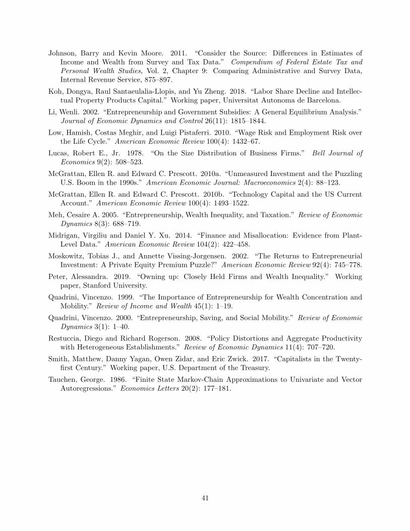
Johnson, Barry and Kevin Moore. 2011. “Consider the Source: Differences in Estimates ofIncome and Wealth from Survey and Tax Data.” Compendium of Federal Estate Tax and

Personal Wealth Studies, Vol. 2, Chapter 9: Comparing Administrative and Survey Data,Internal Revenue Service, 875–897.

Koh, Dongya, Raul Santaeulalia-Llopis, and Yu Zheng. 2018. “Labor Share Decline and Intellec-tual Property Products Capital.” Working paper, Universitat Autonoma de Barcelona.

Li, Wenli. 2002. “Entrepreneurship and Government Subsidies: A General Equilibrium Analysis.”Journal of Economic Dynamics and Control 26(11): 1815–1844.

Low, Hamish, Costas Meghir, and Luigi Pistaferri. 2010. “Wage Risk and Employment Risk overthe Life Cycle.” American Economic Review 100(4): 1432–67.

Lucas, Robert E., Jr. 1978. “On the Size Distribution of Business Firms.” Bell Journal of

Economics 9(2): 508–523.

McGrattan, Ellen R. and Edward C. Prescott. 2010a. “Unmeasured Investment and the PuzzlingU.S. Boom in the 1990s.” American Economic Journal: Macroeconomics 2(4): 88–123.

McGrattan, Ellen R. and Edward C. Prescott. 2010b. “Technology Capital and the US CurrentAccount.” American Economic Review 100(4): 1493–1522.

Meh, Cesaire A. 2005. “Entrepreneurship, Wealth Inequality, and Taxation.” Review of Economic

Dynamics 8(3): 688–719.

Midrigan, Virgiliu and Daniel Y. Xu. 2014. “Finance and Misallocation: Evidence from Plant-Level Data.” American Economic Review 104(2): 422–458.

Moskowitz, Tobias J., and Annette Vissing-Jorgensen. 2002. “The Returns to EntrepreneurialInvestment: A Private Equity Premium Puzzle?” American Economic Review 92(4): 745–778.

Peter, Alessandra. 2019. “Owning up: Closely Held Firms and Wealth Inequality.” Workingpaper, Stanford University.

Quadrini, Vincenzo. 1999. “The Importance of Entrepreneurship for Wealth Concentration andMobility.” Review of Income and Wealth 45(1): 1–19.

Quadrini, Vincenzo. 2000. “Entrepreneurship, Saving, and Social Mobility.” Review of Economic

Dynamics 3(1): 1–40.

Restuccia, Diego and Richard Rogerson. 2008. “Policy Distortions and Aggregate Productivitywith Heterogeneous Establishments.” Review of Economic Dynamics 11(4): 707–720.

Smith, Matthew, Danny Yagan, Owen Zidar, and Eric Zwick. 2017. “Capitalists in the Twenty-first Century.” Working paper, U.S. Department of the Treasury.

Tauchen, George. 1986. “Finite State Markov-Chain Approximations to Univariate and VectorAutoregressions.” Economics Letters 20(2): 177–181.

41

Figure 1. Business Age Profile

42

Figure 2. Sweat Capital By Age

43

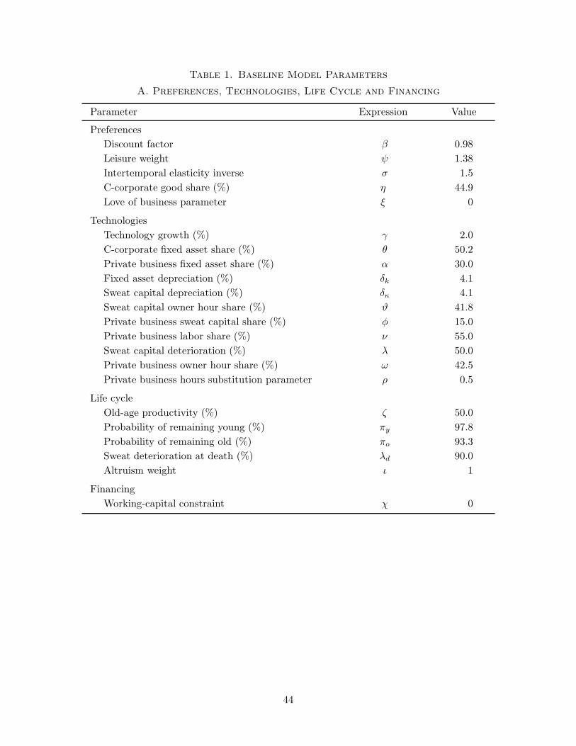
Table 1. Baseline Model Parameters

A. Preferences, Technologies, Life Cycle and Financing

Parameter Expression Value

Preferences

Discount factor β 0.98

Leisure weight ψ 1.38

Intertemporal elasticity inverse σ 1.5

C-corporate good share (%) η 44.9

Love of business parameter ξ 0

Technologies

Technology growth (%) γ 2.0

C-corporate fixed asset share (%) θ 50.2

Private business fixed asset share (%) α 30.0

Fixed asset depreciation (%) δk 4.1

Sweat capital depreciation (%) δκ 4.1

Sweat capital owner hour share (%) ϑ 41.8

Private business sweat capital share (%) φ 15.0

Private business labor share (%) ν 55.0

Sweat capital deterioration (%) λ 50.0

Private business owner hour share (%) ω 42.5

Private business hours substitution parameter ρ 0.5

Life cycle

Old-age productivity (%) ζ 50.0

Probability of remaining young (%) πy 97.8

Probability of remaining old (%) πo 93.3

Sweat deterioration at death (%) λd 90.0

Altruism weight ι 1

Financing

Working-capital constraint χ 0

44

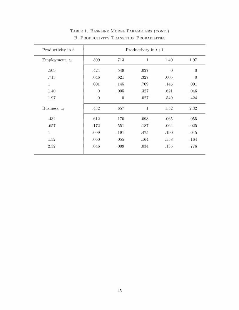
Table 1. Baseline Model Parameters (cont.)

B. Productivity Transition Probabilities

Productivity in t Productivity in t+1

Employment, ǫt .509 .713 1 1.40 1.97

.509 .424 .549 .027 0 0

.713 .046 .621 .327 .005 0

1 .001 .145 .709 .145 .001

1.40 0 .005 .327 .621 .046

1.97 0 0 .027 .549 .424

Business, zt .432 .657 1 1.52 2.32

.432 .612 .170 .098 .065 .055

.657 .172 .551 .187 .064 .025

1 .099 .191 .475 .190 .045

1.52 .060 .055 .164 .558 .164

2.32 .046 .009 .034 .135 .776

45

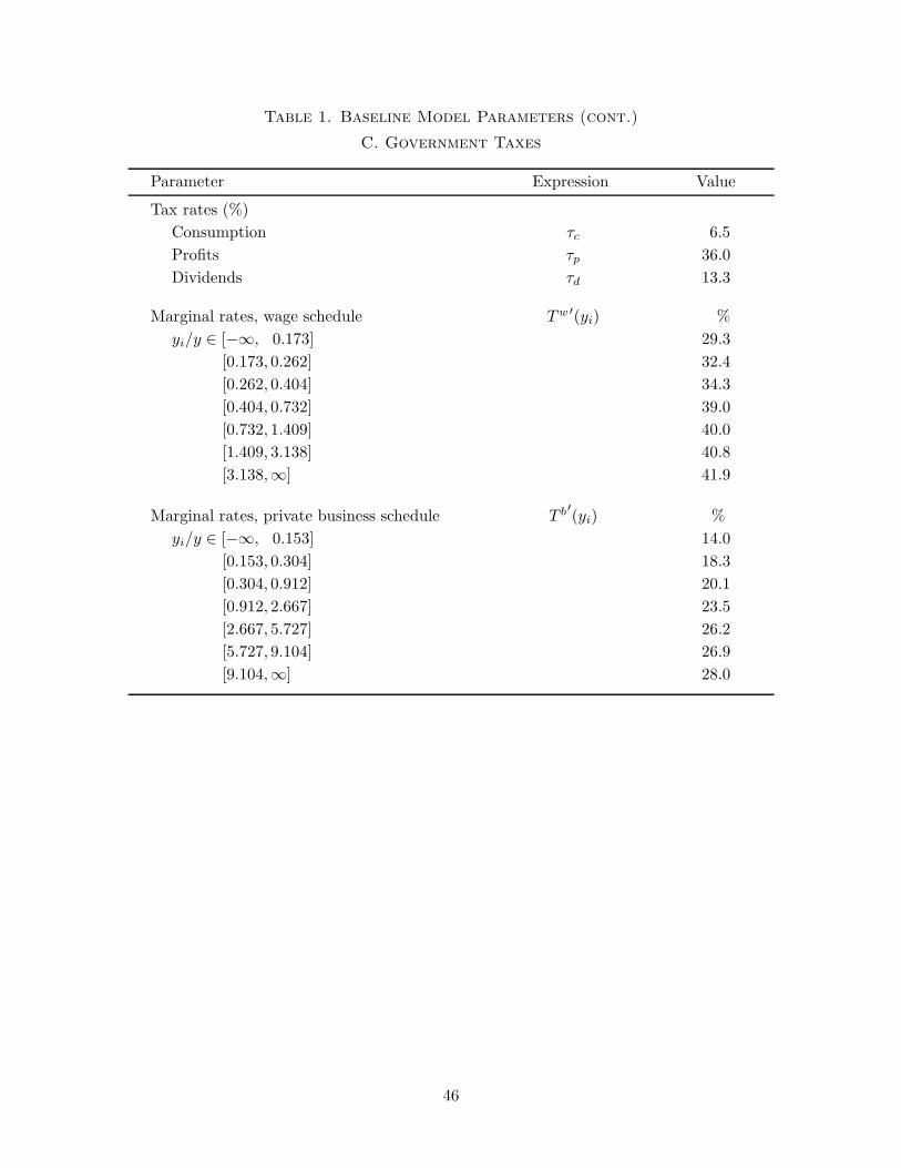
Table 1. Baseline Model Parameters (cont.)

C. Government Taxes

Parameter Expression Value

Tax rates (%)

Consumption τc 6.5

Profits τp 36.0

Dividends τd 13.3

Marginal rates, wage schedule Tw′(yi) %

yi/y ∈ [−∞, 0.173] 29.3

[0.173, 0.262] 32.4

[0.262, 0.404] 34.3

[0.404, 0.732] 39.0

[0.732, 1.409] 40.0

[1.409, 3.138] 40.8

[3.138,∞] 41.9

Marginal rates, private business schedule T b′

(yi) %

yi/y ∈ [−∞, 0.153] 14.0

[0.153, 0.304] 18.3

[0.304, 0.912] 20.1

[0.912, 2.667] 23.5

[2.667, 5.727] 26.2

[5.727, 9.104] 26.9

[9.104,∞] 28.0

46

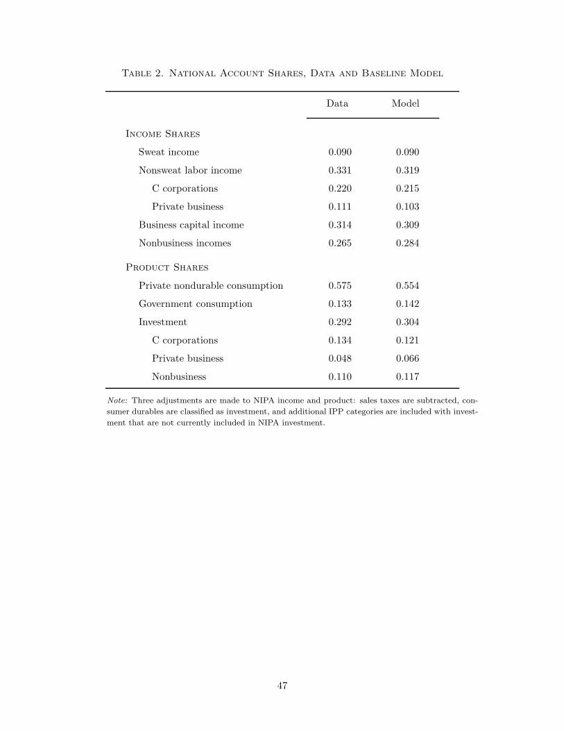
Table 2. National Account Shares, Data and Baseline Model

Data Model

Income Shares

Sweat income 0.090 0.090

Nonsweat labor income 0.331 0.319

C corporations 0.220 0.215

Private business 0.111 0.103

Business capital income 0.314 0.309

Nonbusiness incomes 0.265 0.284

Product Shares

Private nondurable consumption 0.575 0.554

Government consumption 0.133 0.142

Investment 0.292 0.304

C corporations 0.134 0.121

Private business 0.048 0.066

Nonbusiness 0.110 0.117

Note: Three adjustments are made to NIPA income and product: sales taxes are subtracted, con-

sumer durables are classified as investment, and additional IPP categories are included with invest-

ment that are not currently included in NIPA investment.

47

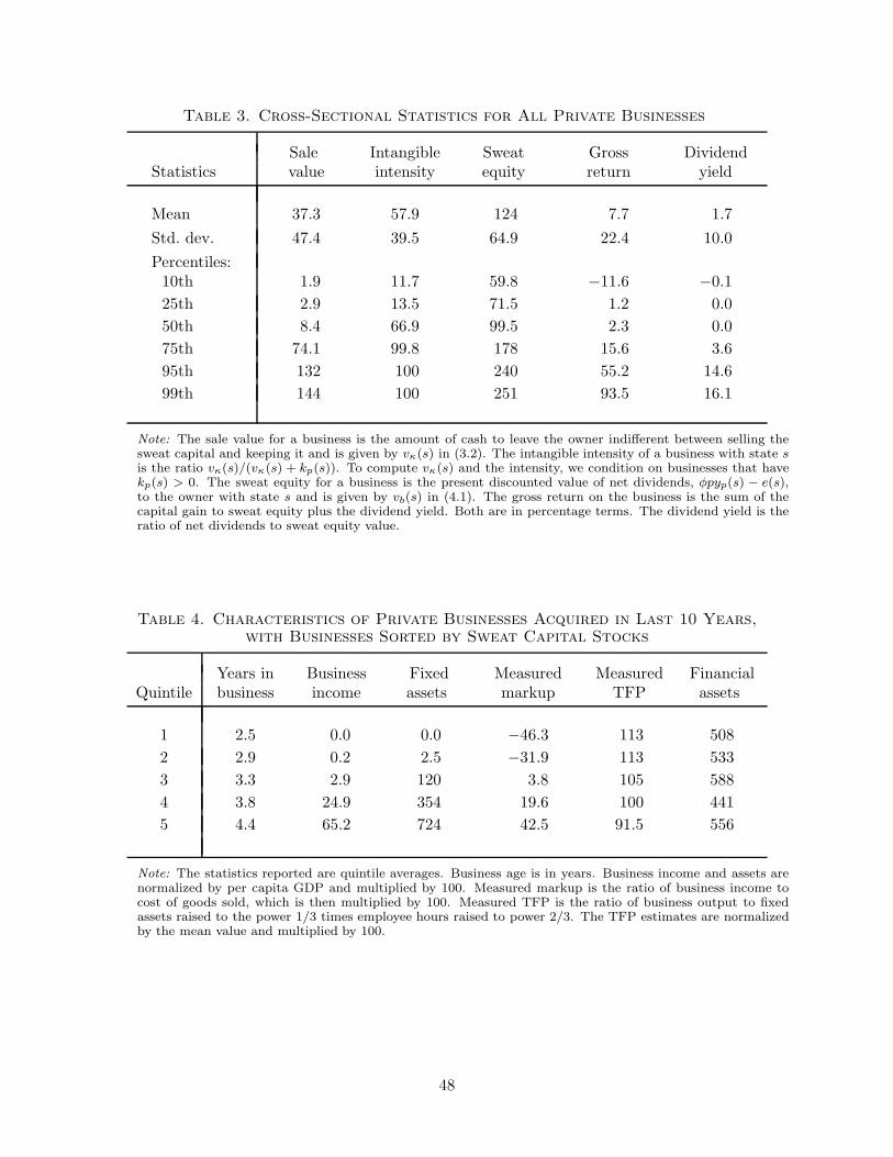
Table 3. Cross-Sectional Statistics for All Private Businesses

Sale Intangible Sweat Gross DividendStatistics value intensity equity return yield

Mean 37.3 57.9 124 7.7 1.7

Std. dev. 47.4 39.5 64.9 22.4 10.0

Percentiles:10th 1.9 11.7 59.8 −11.6 −0.1

25th 2.9 13.5 71.5 1.2 0.0

50th 8.4 66.9 99.5 2.3 0.0

75th 74.1 99.8 178 15.6 3.6

95th 132 100 240 55.2 14.6

99th 144 100 251 93.5 16.1

Note: The sale value for a business is the amount of cash to leave the owner indifferent between selling thesweat capital and keeping it and is given by vκ(s) in (3.2). The intangible intensity of a business with state sis the ratio vκ(s)/(vκ(s) + kp(s)). To compute vκ(s) and the intensity, we condition on businesses that havekp(s) > 0. The sweat equity for a business is the present discounted value of net dividends, φpyp(s) − e(s),to the owner with state s and is given by vb(s) in (4.1). The gross return on the business is the sum of thecapital gain to sweat equity plus the dividend yield. Both are in percentage terms. The dividend yield is theratio of net dividends to sweat equity value.

Table 4. Characteristics of Private Businesses Acquired in Last 10 Years,with Businesses Sorted by Sweat Capital Stocks

Years in Business Fixed Measured Measured FinancialQuintile business income assets markup TFP assets

1 2.5 0.0 0.0 −46.3 113 508

2 2.9 0.2 2.5 −31.9 113 533

3 3.3 2.9 120 3.8 105 588

4 3.8 24.9 354 19.6 100 441

5 4.4 65.2 724 42.5 91.5 556

Note: The statistics reported are quintile averages. Business age is in years. Business income and assets arenormalized by per capita GDP and multiplied by 100. Measured markup is the ratio of business income tocost of goods sold, which is then multiplied by 100. Measured TFP is the ratio of business output to fixedassets raised to the power 1/3 times employee hours raised to power 2/3. The TFP estimates are normalizedby the mean value and multiplied by 100.

48

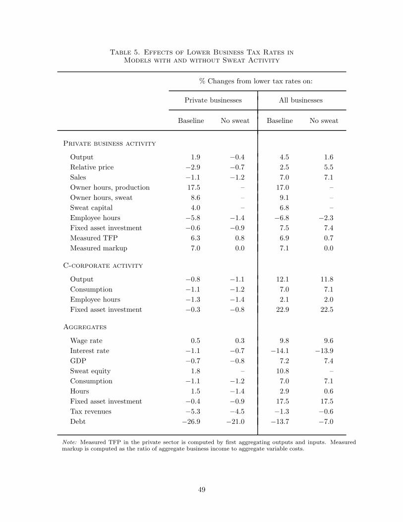
Table 5. Effects of Lower Business Tax Rates inModels with and without Sweat Activity

% Changes from lower tax rates on:

Private businesses All businesses

Baseline No sweat Baseline No sweat

Private business activity

Output 1.9 −0.4 4.5 1.6

Relative price −2.9 −0.7 2.5 5.5

Sales −1.1 −1.2 7.0 7.1

Owner hours, production 17.5 – 17.0 –

Owner hours, sweat 8.6 – 9.1 –

Sweat capital 4.0 – 6.8 –

Employee hours −5.8 −1.4 −6.8 −2.3

Fixed asset investment −0.6 −0.9 7.5 7.4

Measured TFP 6.3 0.8 6.9 0.7

Measured markup 7.0 0.0 7.1 0.0

C-corporate activity

Output −0.8 −1.1 12.1 11.8

Consumption −1.1 −1.2 7.0 7.1

Employee hours −1.3 −1.4 2.1 2.0

Fixed asset investment −0.3 −0.8 22.9 22.5

Aggregates

Wage rate 0.5 0.3 9.8 9.6

Interest rate −1.1 −0.7 −14.1 −13.9

GDP −0.7 −0.8 7.2 7.4

Sweat equity 1.8 – 10.8 –

Consumption −1.1 −1.2 7.0 7.1

Hours 1.5 −1.4 2.9 0.6

Fixed asset investment −0.4 −0.9 17.5 17.5

Tax revenues −5.3 −4.5 −1.3 −0.6

Debt −26.9 −21.0 −13.7 −7.0

Note: Measured TFP in the private sector is computed by first aggregating outputs and inputs. Measuredmarkup is computed as the ratio of aggregate business income to aggregate variable costs.

49

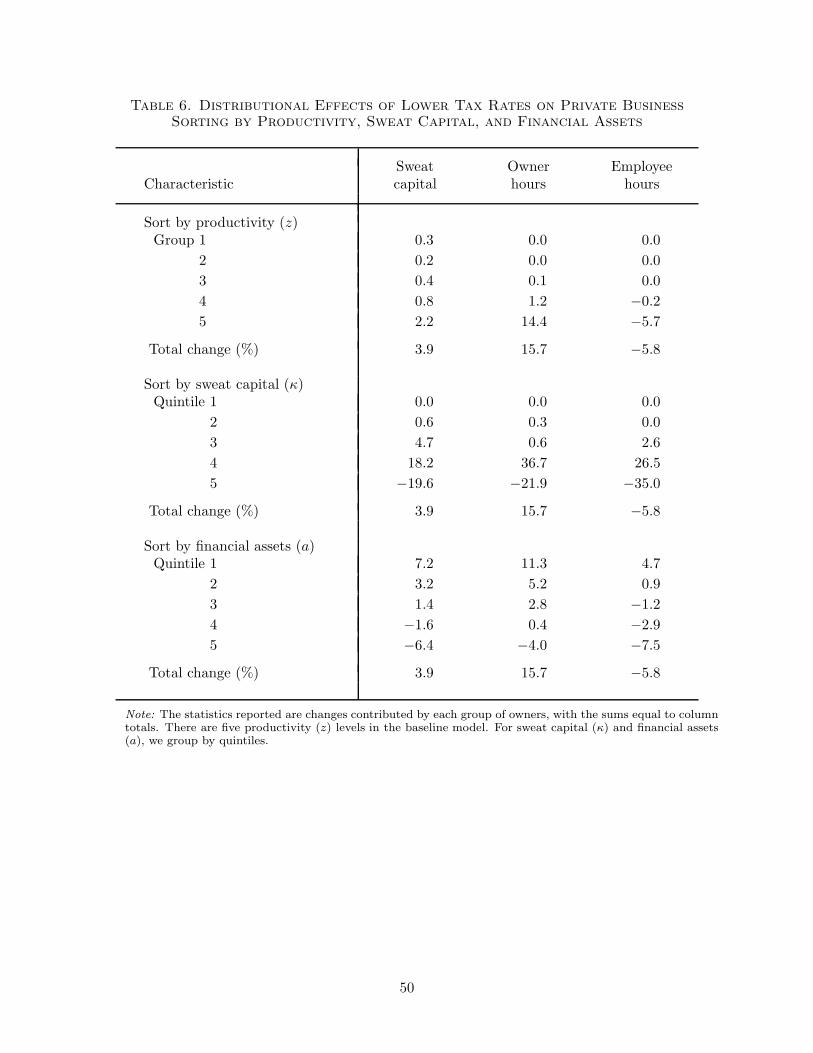
Table 6. Distributional Effects of Lower Tax Rates on Private BusinessSorting by Productivity, Sweat Capital, and Financial Assets

Sweat Owner EmployeeCharacteristic capital hours hours

Sort by productivity (z)Group 1 0.3 0.0 0.0

2 0.2 0.0 0.0

3 0.4 0.1 0.0

4 0.8 1.2 −0.2

5 2.2 14.4 −5.7

Total change (%) 3.9 15.7 −5.8

Sort by sweat capital (κ)Quintile 1 0.0 0.0 0.0

2 0.6 0.3 0.0

3 4.7 0.6 2.6

4 18.2 36.7 26.5

5 −19.6 −21.9 −35.0

Total change (%) 3.9 15.7 −5.8

Sort by financial assets (a)Quintile 1 7.2 11.3 4.7

2 3.2 5.2 0.9

3 1.4 2.8 −1.2

4 −1.6 0.4 −2.9

5 −6.4 −4.0 −7.5

Total change (%) 3.9 15.7 −5.8

Note: The statistics reported are changes contributed by each group of owners, with the sums equal to columntotals. There are five productivity (z) levels in the baseline model. For sweat capital (κ) and financial assets(a), we group by quintiles.

50

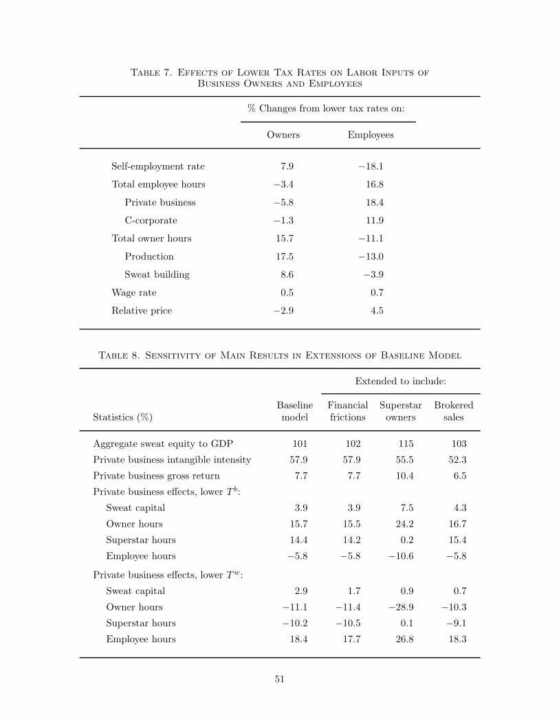
Table 7. Effects of Lower Tax Rates on Labor Inputs ofBusiness Owners and Employees

% Changes from lower tax rates on:

Owners Employees

Self-employment rate 7.9 −18.1

Total employee hours −3.4 16.8

Private business −5.8 18.4

C-corporate −1.3 11.9

Total owner hours 15.7 −11.1

Production 17.5 −13.0

Sweat building 8.6 −3.9

Wage rate 0.5 0.7

Relative price −2.9 4.5

Table 8. Sensitivity of Main Results in Extensions of Baseline Model

Extended to include:

Baseline Financial Superstar BrokeredStatistics (%) model frictions owners sales

Aggregate sweat equity to GDP 101 102 115 103

Private business intangible intensity 57.9 57.9 55.5 52.3

Private business gross return 7.7 7.7 10.4 6.5

Private business effects, lower T b:

Sweat capital 3.9 3.9 7.5 4.3

Owner hours 15.7 15.5 24.2 16.7

Superstar hours 14.4 14.2 0.2 15.4

Employee hours −5.8 −5.8 −10.6 −5.8

Private business effects, lower Tw:

Sweat capital 2.9 1.7 0.9 0.7

Owner hours −11.1 −11.4 −28.9 −10.3

Superstar hours −10.2 −10.5 0.1 −9.1

Employee hours 18.4 17.7 26.8 18.3

51