Participation in Higher Education: Equity and Access

– Are Equity-based Scholarships an Answer?

Buly A. Cardak and

Chris Ryan

Discussion Paper No. A07.03 ISBN 1 92137 7136 ISSN 1441 3213 August 2007

Participation in Higher Education: Equity and Access

— Are Equity–based Scholarships an Answer?∗

Buly A. Cardak† Chris Ryan‡

August 2007

Abstract

We reanalyse data used by Le and Miller (2005), where it is found that studentsfrom low socioeconomic status (SES) backgrounds have lower university participationrates than those from higher SES backgrounds. We utilise the concept of eligibilityto attend university - here defined by both possession of a valid ENTER score andthe value of that score. We find participation among those with similar eligibility toattend university does not vary by SES. Conditional on their ENTER scores, studentsfrom poor family backgrounds are as likely to attend university as those from better-resourced families. Hence, we see little scope for equity–based tuition scholarshipsto rectify differences in participation between these groups. Instead, we find thatpossession and the quality of ENTER scores (eligibility) does rise with SES. Furtheranalysis and policy targeting of the linkage between SES and ENTER scores is morelikely to produce superior equity and access outcomes in higher education.

Keywords: university participation; credit constraints; SES based scholarships.JEL classification numbers: I210, I220, I280.

∗We are grateful for comments and suggestions from David Prentice and Roger Wilkins. Any remainingerrors are our own.

†Department of Economics and Finance, La Trobe University, 3086, Victoria, Australia. Ph:+61 3 94793419, Fax: +61 3 9479 1654, Email: b.cardak@latrobe.edu.au. Cardak acknowledges support from a researchgrant provided by the Australian Research Council (DP0662909).

‡Social Policy Evaluation, Analysis and Research Centre, RSSS, Australian National University, ACT0200, Australia. Ph: +61 2 6125 3881, Fax: +61 2 6125 0182, Email: Chris.Ryan@anu.edu.au. Ryanacknowledges support from a research grant provided by the Australian Research Council (DP0346479).

1 Introduction

It is well established in Australia and internationally that students from lower socioeconomic

status (SES) backgrounds are less likely to attend university than students from higher SES

backgrounds.1 An important question for equity and access in higher education is what

are the causes of this SES imbalance among higher education participants. The intuitive

response is that low SES students have access to limited resources and are credit constrained

when deciding whether or not to attend university. The conclusion is that policy should

rectify this situation by lowering university tuition charges to such students.

The causes of this pattern of enrolment were studied in this journal by Le and Miller

(2005). They found that even among students who completed Year 12, transition rates to

university exhibited a positive socioeconomic status gradient. Consequently, they concluded

that “Addressing the socioeconomic imbalance within the tertiary sector in the current era

would seem to require equity–based scholarships or university fee rebates to be provided to

Year 12 graduates”(page 162).

In this comment, we reconsider the analysis of Le and Miller (2005) and conclude that

policy instruments such as equity–based scholarships or university fee rebates are unlikely

to have much impact on the low university participation of students from poor families.

Using the same data as in Le and Miller (2005) – the 2002 respondents of the 1995 Year

9 cohort of the Longitudinal Surveys of Australian Youth (LSAY) series – we invoke the

notion of ‘eligibility’ and find that students who are ‘eligible’ to attend university are as

likely to attend university if they are from poor family backgrounds as rich. In our analysis,

eligibility encompasses both whether an individual earns a valid tertiary entrance (ENTER)

score and its value. The intuition is relatively straightforward, even very wealthy students

cannot attend university if they do not have a valid ENTER or if their ENTER is of a very

low standard. Thus, high school achievement must complement credit constraints in any

1This evidence can be found in Heckman (2000) and Carneiro and Heckman (2002) for the United States,Greenaway and Haynes (2003), Galindo–Rueda et al. (2004) and Dearden et al. (2004) for the UK, Chapmanand Ryan (2005) and Le and Miller (2005) for Australia and Finnie and Laporte (2003) for Canada, whileBlossfeld and Shavit (1993) provide a collection of studies with evidence on a further 13 countries.

1

analysis of differences in university participation rates by SES. We find that it is whether

individuals obtain an ENTER score and its value, even among those who complete Year 12,

that drives a wedge between the university participation rates of students from rich and poor

family backgrounds — not differing rates of participation among those who are eligible.2

The next Section provides a probability decomposition that highlights the differences

between our empirical approach and that of Le and Miller (2005). Our results are described

in Section 3, with our interpretation of these results and concluding remarks in Section 4.

2 Estimation Methodology

In this section we present two decompositions of the probability that individuals attend

university. We do this in order to highlight an alternative interpretation of the results

presented in Le and Miller (2005). The first is our characterisation of the Le and Miller

results and the way they interpret them. While our representation does not appear in

their paper, it neatly captures the way they interpreted their results. We then present

an alternative probability decomposition of university participation that incorporates the

concept of eligibility. This reflects the need for students to satisfy some minimum standard

for consideration for entry to university. In Australia, this minimum requirement is an

ENTER score.

Denote university participation by individual i by the dummy variable, ui. Let si = 1

indicate individual i has completed school. The probability a recent school graduate attends

university can be expressed as:3

2A related paper, Cardak and Ryan (2006), analyses university participation using data from a latercohort of students. It splits the student population into distinct groups based on student and school SEScharacteristics and reaches qualitatively similar conclusions to those reached here – individuals from thelowest SES group are as likely to go to university as the top group, conditional on the ENTER scores theyachieve. However, on average, students from the lowest SES group tend to obtain substantially lower ENTERscores than those from higher SES groups.

3From the law of total probability there is another term on the right hand side of equation (1),Prob[u| w, s = 0] × Prob[s = 0| w]. However, among the school leavers studied here only those whocomplete Year 12 can attend university, so Prob[u| w, s = 0] = 0.

2

Prob[u] =

∫ w

w

Prob[u| w, s = 1]× Prob[s = 1| w]× fw(w) dw. (1)

where w ∈ [w,w] measures socioeconomic status (SES) and the pdf of w is given by fw(w).

The proportion of students attending university for any given SES level is the product of

the ‘continuation rate’ among Year 12 completers, Prob[u| w, s = 1], and the proportion

of Year 12 completers with that given SES level, Prob[s = 1| w]. Le and Miller (2005) find

both these rates exhibit a positive socioeconomic gradient, that is ∂Prob[u| w, s=1]∂w

> 0 and

∂Prob[s=1| w]∂w

> 0 – see for example columns (ii) and (iii) in Table 3 in Le and Miller (2005).

Since both of these elements increase with w, ∂Prob[u]∂w

> 0.

The key innovation in our analysis is the recognition that in order to matriculate, students

need to do more than simply complete Year 12. Students who undertake Year 12 studies are

not eligible for formal ‘Certificates’ from their state school certificate accrediting agencies if,

for example, they undertake too many vocational subjects. Universities, in addition, do not

admit students randomly from those who complete Year 12. Rather, students are admitted

on the basis of their relative rank within their cohort, based on assessments of their rank

known generically as their Equivalent National Tertiary Entrance Rank or ENTER score.

In order to be considered for a university place, we assume that a student must possess such

an ENTER score, which we view as a basic eligibility requirement that informs our analysis

of university entrance.4

Denote an individual’s observed university entrance score by yi. We assume that yi is

determined by the innate ability of individuals, ai, and their socioeconomic background, that

is yi = λ(wi, ai). Denote an indicator variable by r, which takes the value 1 if an individual

obtains a valid ENTER score, between the values y and y, and 0 otherwise. Finally, assume

that the density of yi is given by gy(y). With this notation, we can decompose the first term

of equation (1), the probability individuals attend university conditional on their SES (wi)

and having completed Year 12 (si = 1) as:

4Admission to university on the basis of ENTER scores is the dominant mode for those completing schoolin Australia. Other criteria are used for mature aged entrants.

3

Prob[u| w, s = 1] = Prob[u| w, s = 1, r = 1] × Prob[r = 1| w, s = 1]

=

∫ y

y

Prob[u| w, s = 1, y] × gy(y| w, s = 1) dy ×

Prob [r = 1| w, s = 1] . (2)

Based on equation (2), three factors determine the probability that individuals of a given

SES, who complete school, progress to university. The first is a parameter which reflects the

likelihood of attending university conditional on the individual’s eligibility (ENTER) score

and SES level, Prob[u| w, s = 1, y]. The second is the distribution of ENTER scores among

this group gy(y| w, s = 1). The remaining factor reflects the likelihood individuals obtain an

ENTER score (r = 1), given their completion of Year 12 and SES level, Prob[r = 1| w, s = 1].

Linking equation (2) with equation (1), we have decomposed the first term on the right

hand side of equation (1) into the three factors identified in equation (2). While the prob-

ability of obtaining an ENTER score among those completing Year 12 may vary by social

background, the analysis of the potential gains from SES–based scholarships must focus on

those students with ENTER scores, that is, those students eligible to go to university.5 We

view the key question to be whether or not ∂Prob[u|w,s=1,y]∂w

> 0, that is, given a student’s

ENTER score, is the student more likely to attend university, the higher their SES (wi). If

this is the case, SES–based scholarships have the potential to increase participation among

low–SES groups. Otherwise, they do not and would simply tend to provide funds to those

low–SES individuals who would have gone to university anyway.6

In the section that follows, we represent graphically how the functions Prob[u|w, s =

1, y] (for those with valid ENTER scores) and Prob[r = 1|w, s = 1] and the probability

individuals complete Year 12, Prob[s = 1|w], vary with SES (w). These figures are based on

5We explore below the scope for SES–based scholarships to affect the proportion completing Year 12 and,of those, the proportion who obtain an ENTER score.

6The complete statement of the derivative ∂Prob[u|w,s=1]∂w would require application of the chain and

multiplication rules of differentiation to equation (2). Our discussion above focusses on whether the terminvolving ∂Prob[u|w,s=1,y]

∂w makes a relatively large contribution to it.

4

conditional means that we estimate non-parametrically, drawing on the approach of Barsky

et al. (2002).7

3 Results

3.1 Diagrams

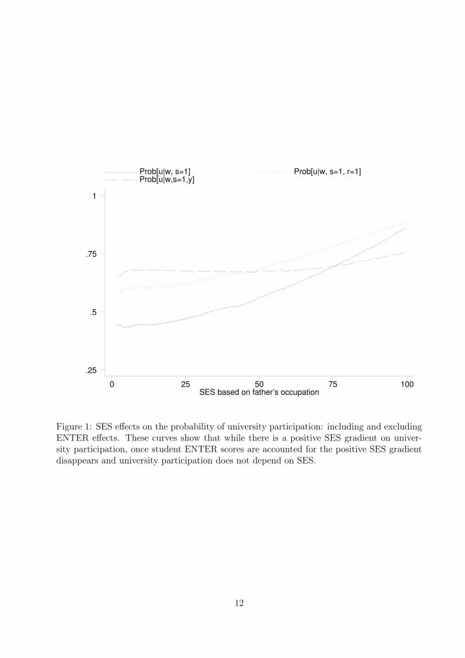
In Figure 1 we plot three probabilities of attending university and show how these probabili-

ties change with SES. The first (solid) curve represents Prob[u|w, s = 1], which derives from

equation (1) and reflects the approach taken in Le and Miller (2005). This curve is consistent

with the results in Le and Miller (2005) - the probability of attending university is increas-

ing in SES, given high school completion (s = 1). The second (dotted) curve is similar, but

is estimated only for individuals with a valid ENTER score (r = 1), so the probability of

university participation is higher among this group, but the curve displays the same positive

relationship with SES. The third (dashed) curve represents Prob [u|w, s = 1, y], which de-

rives from our decomposition in equation (2). This curve is relatively flat, implying there is

little or no relationship between university participation and SES, after controlling for high

school completion (s = 1) and ENTER scores (y). While this curve appears to increase at

very high levels of parental SES, there are relatively few SES observations above the value

80, so the relationship at these levels is not estimated very precisely.8

The apparent relationship between university participation and SES reflected in the first

curve, Prob[u|w, s = 1], seems to be an indirect one, driven by the effect of SES on ENTER

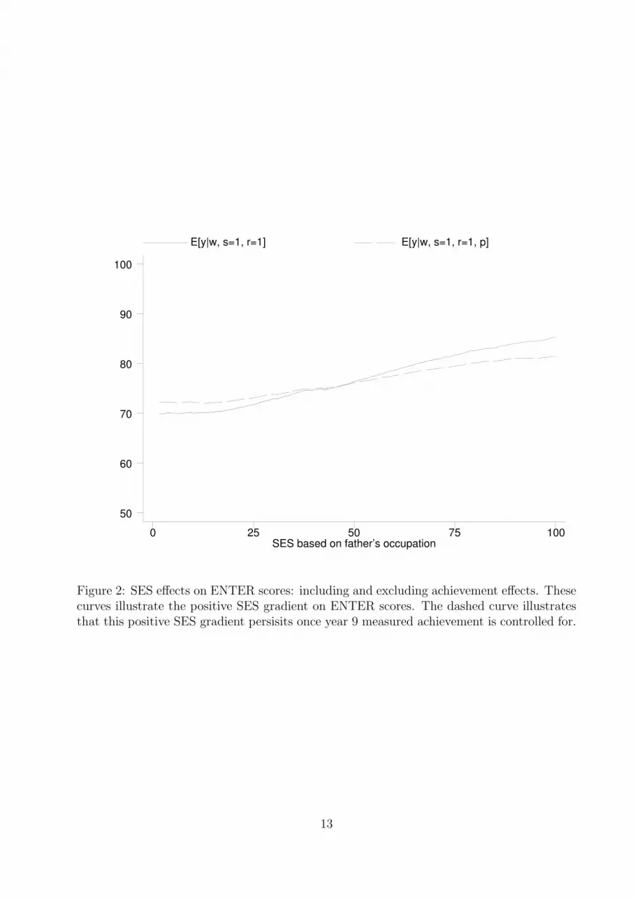
scores. We thus plot the relationship between ENTER scores and SES, E [y|w, s = 1, r = 1],

in Figure 2, where the positive slope of this curve reflects dydw

> 0. The implication is that a

plot of Prob[u|w, s = 1], confounds the behaviour of Prob [u|w, s = 1, y] and E [y|w, s = 1, r = 1]

with respect to SES. We also control for Year 9 achievement (denoted by p and also referred

7We use the mrunning program written by Royston and Cox (2005) in STATA to generate these estimatesof the conditional means.

8Moreover, there was no increase in the curve at high SES values when it was estimated with data from2000, where there were more observations, rather than based on responses from 2002 as in Figure 1.

5

to as “early school achievement” in Le and Miller (2005)) in an attempt to control for in-

nate student ability, by plotting E [y|w, s = 1, r = 1, p] in Figure 2. We find the positive

SES gradient on ENTER scores is robust to this control, though the effect is slightly less

pronounced.

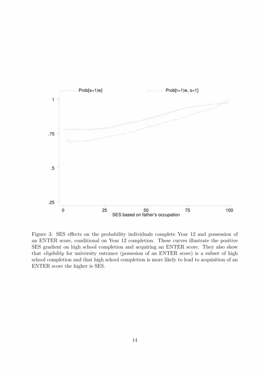
Figure 3 shows how the probability of earning an ENTER score, Prob[r = 1|w, s = 1],

and the probability an individual completes Year 12, Prob[s = 1|w], both vary with SES

(w). Both of these probabilities exhibit a positive relationship with SES. The fact that

Prob[s = 1|w] > Prob[r = 1|w, s = 1] confirms that those matriculating or earning an

ENTER score are a subset of high school completers. From the figure, this gap narrows as

SES increases, suggesting that a smaller proportion of low SES high school completers earn

ENTER scores.

Taken together, this analysis confirms the finding in Le and Miller (2005), that Prob[u|w, s =

1] exhibits a positive SES gradient. However, after controlling for ENTER scores, low SES

students are no less likely to attend university than high SES students. If we analyse the

sources of the positive SES gradient on Prob[u|w, s = 1], we find that not all school com-

pletion is the same. Earned ENTER scores exhibit a positive SES gradient, even after

conditioning for Year 9 achievement. The probability of obtaining an ENTER score also

exhibits a positive SES gradient. In summary, low SES students seem less likely to be eli-

gible for university entrance. Given these insights, we must reconsider if, all else constant,

offering SES-based scholarships will induce more low SES students to attend university. It

would seem that policies need to also consider the matriculation rate and the value of the

ENTER scores earned by students from low SES backgrounds.

3.2 Regression results

Results of regression equations confirm those apparent from the diagrams just presented.

Four distinct equations were estimated of the determinants of:

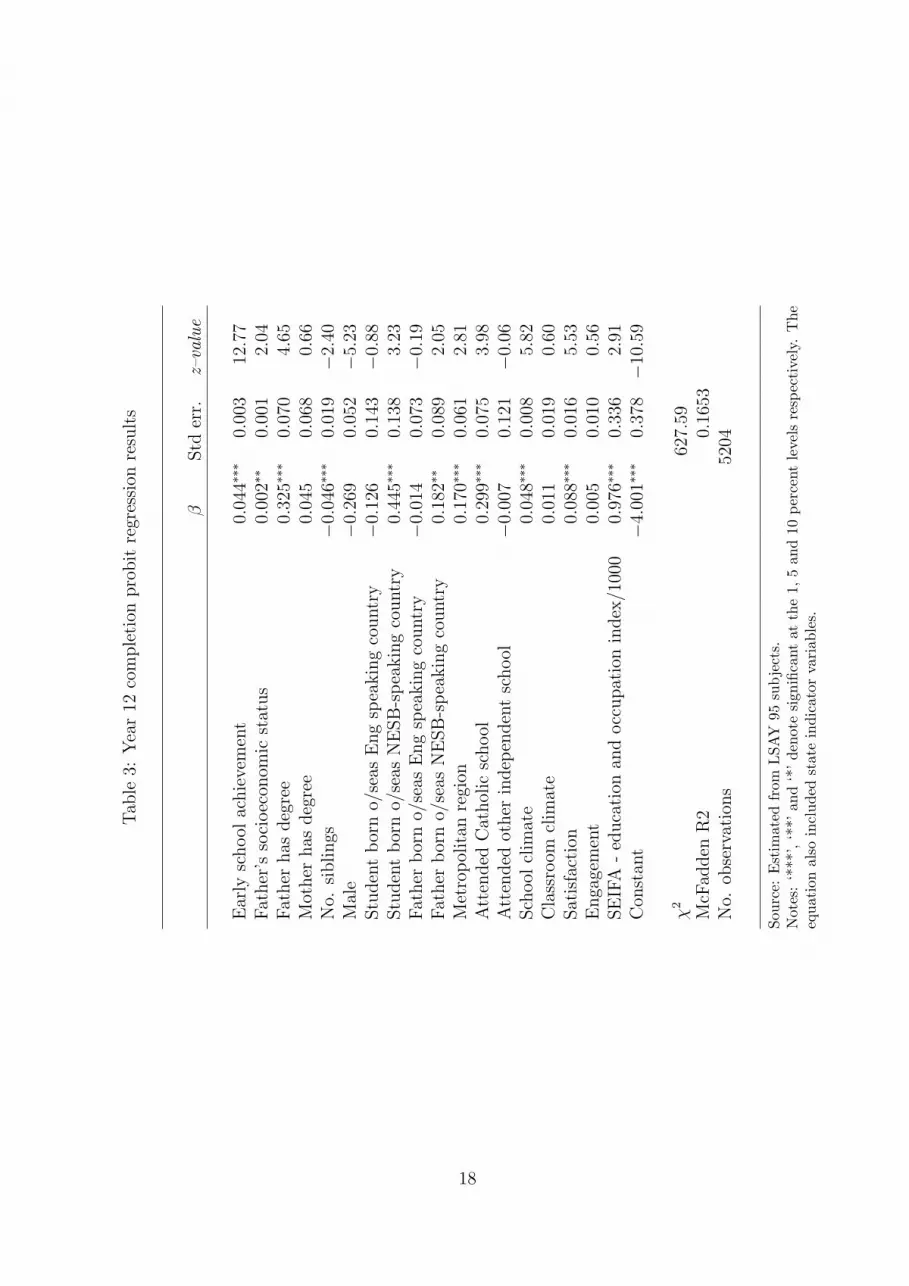
1. Year 12 completion;

6

2. possession of a valid ENTER score, conditional on Year 12 completion;

3. the ENTER score individuals obtained, conditional on possession of a valid ENTER

score; and

4. university participation, conditional on possession of a valid ENTER score.

The first, second and fourth outcomes are binary, so these equations were estimated using

a probit specification. The dependent variable for the third outcome is continuous, albeit

limited to those that report a valid ENTER score. The explanatory variables consisted of

those included in the equations reported in Le and Miller (2005), with broadly similar def-

initions to those used there. The main variable of interest is the SES variable, measured

by the ANU3 scale which reflects the prestige of the occupation in which the father works.9

The key result for this paper is that the father’s SES variable is found to have a positive

and significant coefficient in the first three equations, but not the last. That is, father’s SES

has a positive correlation with Year 12 completion, earning an ENTER score and the level

of that ENTER score, while it plays no statistically significant role in explaining university

participation. These results, specifically the estimated parameter values and their signifi-

cance levels, are summarised in Table 1 and confirm statistically our conclusions drawn from

Figures 1 – 3.

More detailed regression results for the last equation are provided in Table 2, regressed

over those individuals with valid ENTER scores.10 These results show that whether ENTER

score or Year 9 achievement is included in the university participation equation estimated

over those with valid ENTER scores (unlike Le and Miller who include all high school

completers, including those that are not eligible for university), the father’s SES variable

9The ANU 3 scale (Jones 1989) is a status-based occupational prestige measure, which lies between 0 and100. Differences between our analysis and that of Le and Miller (2005) include: (i) they use a more detailedregional breakdown; (ii) we split the overseas birthplace variables into those from English and non-Englishspeaking countries; (iii) we do not include local area unemployment variables. Our results are estimatedusing respondents in 2002, as in Le and Miller (2005).

10Results for the other equations appear in the appendix. Equations were estimated to take account ofselection effects for those obtaining ENTER scores, but these effects were not significant in the universityparticipation equation.

7

is not statistically significant. This confirms the conclusion drawn from Figure 1; given

a student’s ENTER score, which is an important determinant of university participation,

father’s SES does not explain university participation. It also implies that research into

university participation needs to focus more explicitly on the role of SES for university

eligibility, that is, earning an ENTER score and its value. There is one caveat to this

conclusion, however. It is that another element of parental SES remains significant when

the ENTER score is included in the university participation equation – whether or not the

individual’s father has a university degree. Hence, there may be some residual SES effect

on university participation for this group. We note, however, two factors about this effect.

The first is that the ENTER score effect on university participation dominates the father’s

degree effect – the marginal effect of the latter is equivalent to a movement of just 5 points

in the ENTER score. The second is that this residual effect is not evident in data from

the later 1998 cohort of LSAY, while the other qualitative features of the results presented

here are. Hence, we continue to think that it is a better understanding of how SES affects

ENTER scores that is necessary for us to understand its impact on university participation

in Australia.

4 Conclusion

We have studied differences in university participation by SES. As in Le and Miller (2005),

we identified a positive SES gradient on university participation. However, we found that

once we control for student eligibility as measured by possession and quality of ENTER

scores, the positive SES gradient on university participation disappears. We found students

with a given ENTER score are equally likely to attend university irrespective of their SES.

The underlying premise of SES-based scholarships or fee relief is that eligible students are not

attending university. We would expect to see lower participation rates by low SES students

after controlling for ENTER scores if such a policy were to be effective.

Instead, we find that students of low SES are less likely to earn an ENTER score and

8

the ENTER scores they do earn are lower than students of higher SES. If we are interested

in equity and access in higher education and the causes of the SES imbalance among higher

education participants in Australia, we must consider the interaction between SES and eli-

gibility. That is, policy must consider why fewer low SES students earn ENTER scores and

how the ENTER scores these low SES students do earn can be improved. Once eligibility

is addressed, the role for SES-based scholarships or fee relief may need to be reconsidered.

However, given the evidence, SES-based scholarships or fee relief should not currently be at

the top of the list policy instruments when formulating strategies for improving equity and

access in higher education in Australia.

9

References

[1] Barsky, R., Bound, J., Charles, K.K. and J.P. Lupton, (2002), “Accounting for the

Black-White Wealth Gap: A Nonparametric Approach”, Journal of the American Sta-

tistical Association 97, 663-673.

[2] Blossfeld, H-P and Y. Shavit, (1993), Persistent Inequality: Changing Educational At-

tainment in Thirteen Countries, Boulder, San Francisco, Oxford: Westview Press.

[3] Cardak, B. and C. Ryan, (2006), Why are high ability individuals from poor backgrounds

under-represented at university?, School of Business Discussion Paper No. A06.04, La

Trobe University, Melbourne.

[4] Carneiro, P. and J.J. Heckman, (2002), “The Evidence on Credit Constraints in Post-

Secondary Schooling”, The Economic Journal 112, 705-734.

[5] Chapman, B. and C. Ryan, (2005), “The Access Implications of Income Contingent

Charges for Higher Education: Lessons from Australia”, Economics of Education Review

24, 491-512.

[6] Dearden, L., L. McGranahan and B. Sianesi, (2004), “The Role of Credit Constraints in

Educational Choices: Evidence from the NCDS and BSC70”, Centre for the Economics

of Education, London School of Economics, Working Paper CEEDP0048, accessed at

http://cee.lse.ac.uk/cee%20dps/ceedp48.pdf

[7] Finnie, R. and C. Laporte, (2003), “Family Background and Access

to Post-Secondary Education: What Happened in the 1990’s”, School

of Policy Studies, Queens University, Working Paper 34, accessed at

http://www.queensu.ca/sps/working papers/files/sps wp34.pdf

[8] Galindo–Rueda, F., O. Marcenaro–Gutierrez and A. Vignoles, (2004), “The Widening

Socio-economic Gap in UK Higher Education”, Centre for the Economics of Education,

London School of Economics.

10

[9] Greenaway, D. and M. Haynes, (2003), “Funding Higher Education in the UK: The Role

of Fees and Loans”, The Economic Journal 113, F150-F166.

[10] Heckman, J.J., (2000), “Policies to Foster Human Capital”, Research in Economics 54,

3-56.

[11] Jones, F.L., (1989), “Occupational prestige in Australia: A new scale”, Australian and

New Zealand Journal of Sociology 25, 187 - 199.

[12] Le, A.T., and P. W. Miller, (2005), “Participation in Higher Education: Equity and

Access”, Economic Record 81, 152-165.

[13] Royston, P., and N.J. Cox, (2005), “A multivariable scatterplot smoother”, The Stata

Journal 5, 405-412.

11

SES based on father’s occupation

Prob[u|w, s=1] Prob[u|w, s=1, r=1] Prob[u|w,s=1,y]

0 25 50 75 100

.25

.5

.75

1

Figure 1: SES effects on the probability of university participation: including and excludingENTER effects. These curves show that while there is a positive SES gradient on univer-sity participation, once student ENTER scores are accounted for the positive SES gradientdisappears and university participation does not depend on SES.

12

SES based on father’s occupation

E[y|w, s=1, r=1] E[y|w, s=1, r=1, p]

0 25 50 75 100

50

60

70

80

90

100

Figure 2: SES effects on ENTER scores: including and excluding achievement effects. Thesecurves illustrate the positive SES gradient on ENTER scores. The dashed curve illustratesthat this positive SES gradient persisits once year 9 measured achievement is controlled for.

13

SES based on father’s occupation

Prob[s=1|w] Prob[r=1|w, s=1]

0 25 50 75 100

.25

.5

.75

1

Figure 3: SES effects on the probability individuals complete Year 12 and possession ofan ENTER score, conditional on Year 12 completion. These curves illustrate the positiveSES gradient on high school completion and acquiring an ENTER score. They also showthat eligibility for university entrance (possesion of an ENTER score) is a subset of highschool completion and that high school completion is more likely to lead to acquisition of anENTER score the higher is SES.

14

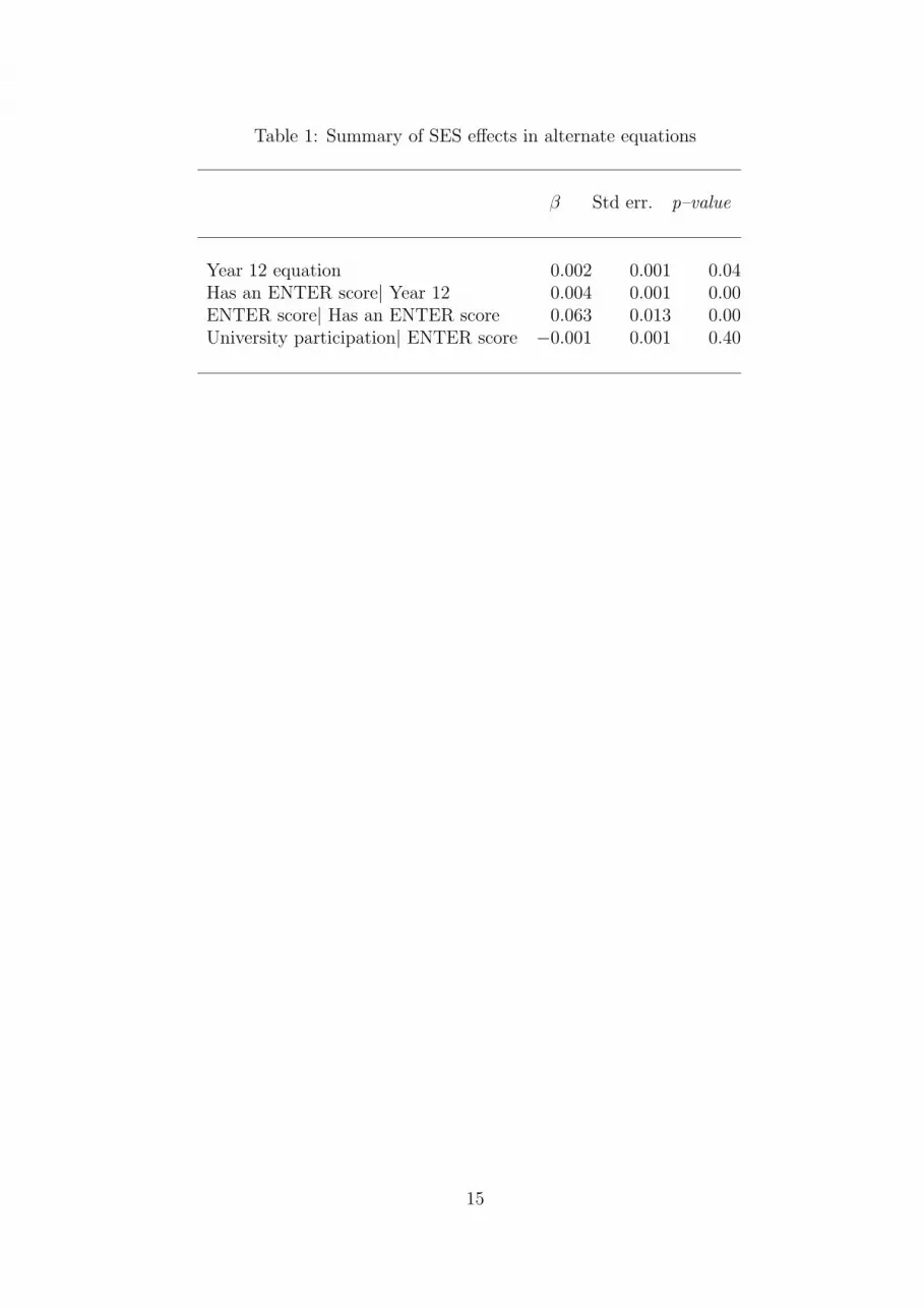
Table 1: Summary of SES effects in alternate equations

β Std err. p–value

Year 12 equation 0.002 0.001 0.04Has an ENTER score| Year 12 0.004 0.001 0.00ENTER score| Has an ENTER score 0.063 0.013 0.00University participation| ENTER score −0.001 0.001 0.40

15

Tab

le2:

Univ

ersi

typar

tici

pat

ion

pro

bit

regr

essi

onre

sult

sam

ong

thos

ew

ith

valid

EN

TE

Rsc

ores

EN

TE

Rin

cluded

Ach

ieve

men

tin

cluded

βStd

err.

z–va

lue

βStd

err.

z–va

lue

Ear

lysc

hool

achie

vem

ent

0.04

4∗∗∗

0.00

411

.30

EN

TE

Rsc

ore

0.05

0∗∗∗

0.00

222

.09

Fat

her

’sso

cioec

onom

icst

atus

−0.0

010.

001

−0.8

50.

001

0.00

11.

06Fat

her

has

deg

ree

0.27

1∗∗∗

0.07

03.

900.

316∗∗∗

0.06

84.

66M

other

has

deg

ree

0.00

20.

077

0.02

0.12

9∗0.

071

1.83

No.

siblings

−0.0

330.

023

−1.4

4−0

.050∗∗∗

0.02

0−2

.53

Mal

e−0

.070

0.05

5−1

.28

−0.1

98∗∗∗

0.05

3−3

.77

Stu

den

tbor

no/

seas

Eng

spea

kin

gco

untr

y−0

.072

0.18

2−0

.39

−0.0

240.

155

−0.1

5Stu

den

tbor

no/

seas

NE

SB

-spea

kin

gco

untr

y0.

287∗∗

0.14

02.

050.

408∗∗∗

0.13

43.

05Fat

her

bor

no/

seas

Eng

spea

kin

gco

untr

y0.

009

0.09

50.

10−0

.107

0.08

1−1

.32

Fat

her

bor

no/

seas

NE

SB

-spea

kin

gco

untr

y0.

136

0.08

81.

550.

197∗∗∗

0.07

82.

51M

etro

pol

itan

regi

on−0

.083

0.07

8−1

.06

−0.0

840.

069

−1.2

1A

tten

ded

Cat

hol

icsc

hool

−0.0

460.

080

−0.5

70.

083

0.07

71.

08A

tten

ded

other

indep

enden

tsc

hool

−0.0

330.

094

−0.3

50.

094

0.09

50.

99Sch

ool

clim

ate

0.02

2∗∗

0.01

12.

110.

043∗∗∗

0.00

94.

61C

lass

room

clim

ate

−0.0

280.

019

−1.4

70.

000

0.01

80.

01Sat

isfa

ctio

n0.

064∗∗∗

0.01

83.

580.

056∗∗∗

0.01

73.

33E

nga

gem

ent

0.01

20.

010

1.18

0.01

6∗0.

009

1.74

SE

IFA

-ed

uca

tion

and

occ

upat

ion

index

/100

00.

032

0.37

00.

090.

497

0.34

01.

46C

onst

ant

−4.3

65∗∗∗

0.44

0−9

.93

−4.0

61∗∗∗

0.43

0−9

.45

χ2

759.

438

9.4

McF

adden

R2

0.29

0.12

No.

obse

rvat

ions

3126

3121

Sour

ce:

Est

imat

edfr

omLSA

Y95

subje

cts.

Not

es:

‘***

’,‘*

*’an

d‘*

’de

note

sign

ifica

ntat

the

1,5

and

10pe

rcen

tle

vels

resp

ecti

vely

.T

heeq

uati

ons

also

incl

uded

stat

ein

dica

tor

vari

able

s.

16

Appendix: Supplementary regression results

17

Tab

le3:

Yea

r12

com

ple

tion

pro

bit

regr

essi

onre

sult

s

βStd

err.

z–va

lue

Ear

lysc

hool

achie

vem

ent

0.04

4∗∗∗

0.00

312

.77

Fat

her

’sso

cioec

onom

icst

atus

0.00

2∗∗

0.00

12.

04Fat

her

has

deg

ree

0.32

5∗∗∗

0.07

04.

65M

other

has

deg

ree

0.04

50.

068

0.66

No.

siblings

−0.0

46∗∗∗

0.01

9−2

.40

Mal

e−0

.269

0.05

2−5

.23

Stu

den

tbor

no/

seas

Eng

spea

kin

gco

untr

y−0

.126

0.14

3−0

.88

Stu

den

tbor

no/

seas

NE

SB

-spea

kin

gco

untr

y0.

445∗∗∗

0.13

83.

23Fat

her

bor

no/

seas

Eng

spea

kin

gco

untr

y−0

.014

0.07

3−0

.19

Fat

her

bor

no/

seas

NE

SB

-spea

kin

gco

untr

y0.

182∗∗

0.08

92.

05M

etro

pol

itan

regi

on0.

170∗∗∗

0.06

12.

81A

tten

ded

Cat

hol

icsc

hool

0.29

9∗∗∗

0.07

53.

98A

tten

ded

other

indep

enden

tsc

hool

−0.0

070.

121

−0.0

6Sch

ool

clim

ate

0.04

8∗∗∗

0.00

85.

82C

lass

room

clim

ate

0.01

10.

019

0.60

Sat

isfa

ctio

n0.

088∗∗∗

0.01

65.

53E

nga

gem

ent

0.00

50.

010

0.56

SE

IFA

-ed

uca

tion

and

occ

upat

ion

index

/100

00.

976∗∗∗

0.33

62.

91C

onst

ant

−4.0

01∗∗∗

0.37

8−1

0.59

χ2

627.

59M

cFad

den

R2

0.16

53N

o.ob

serv

atio

ns

5204

Sour

ce:

Est

imat

edfr

omLSA

Y95

subje

cts.

Not

es:

‘***

’,‘*

*’an

d‘*

’de

note

sign

ifica

ntat

the

1,5

and

10pe

rcen

tle

vels

resp

ecti

vely

.T

heeq

uati

onal

soin

clud

edst

ate

indi

cato

rva

riab

les.

18

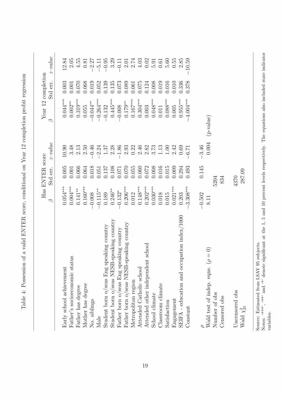
Tab

le4:

Pos

sess

ion

ofa

valid

EN

TE

Rsc

ore,

condit

ional

onY

ear

12co

mple

tion

pro

bit

regr

essi

on

Has

EN

TE

Rsc

ore

Yea

r12

com

ple

tion

βStd

err.

z–va

lue

βStd

err.

z–va

lue

Ear

lysc

hool

achie

vem

ent

0.05

4∗∗∗

0.00

510

.90

0.04

4∗∗∗

0.00

312

.84

Fat

her

’sso

cioec

onom

icst

atus

0.00

4∗∗∗

0.00

13.

480.

002∗∗

0.00

12.

05Fat

her

has

deg

ree

0.14

1∗∗

0.06

62.

130.

319∗∗∗

0.07

04.

55M

other

has

deg

ree

0.16

0∗∗∗

0.06

42.

500.

055

0.06

80.

81N

o.si

blings

−0.0

080.

018

−0.4

6−0

.044∗∗

0.01

9−2

.27

Mal

e−0

.115∗∗

0.05

1−2

.24

−0.2

64∗∗∗

0.05

2−5

.11

Stu

den

tbor

no/

seas

Eng

spea

kin

gco

untr

y0.

189

0.13

71.

37−0

.132

0.13

9−0

.95

Stu

den

tbor

no/

seas

NE

SB

-spea

kin

gco

untr

y0.

246∗∗

0.10

82.

280.

445∗∗∗

0.13

53.

29Fat

her

bor

no/

seas

Eng

spea

kin

gco

untr

y−0

.132∗

0.07

1−1

.86

−0.0

080.

073

−0.1

1Fat

her

bor

no/

seas

NE

SB

-spea

kin

gco

untr

y0.

206∗∗∗

0.07

02.

930.

179∗∗

0.08

92.

01M

etro

pol

itan

regi

on0.

012

0.05

50.

220.

167∗∗∗

0.06

12.

74A

tten

ded

Cat

hol

icsc

hool

0.14

8∗∗∗

0.06

02.

460.

304∗∗∗

0.07

54.

03A

tten

ded

other

indep

enden

tsc

hool

0.20

2∗∗∗

0.07

22.

820.

003

0.12

40.

02Sch

ool

clim

ate

0.03

0∗∗∗

0.00

83.

730.

048∗∗∗

0.00

85.

91C

lass

room

clim

ate

0.01

80.

016

1.13

0.01

10.

019

0.61

Sat

isfa

ctio

n0.

015

0.01

51.

000.

088∗∗∗

0.01

65.

60E

nga

gem

ent

0.02

1∗∗∗

0.00

92.

420.

005

0.01

00.

55SE

IFA

-ed

uca

tion

and

occ

upat

ion

index

/100

00.

203

0.29

40.

690.

955∗∗∗

0.33

62.

85C

onst

ant

−3.3

08∗∗∗

0.49

3−6

.71

−4.0

04∗∗∗

0.37

8−1

0.59

ρ−0

.502

0.14

5−3

.46

Wal

dte

stof

indep

.eq

ns.

(ρ=

0)8.

110.

004

(p-v

alue)

Num

ber

ofob

s52

04C

enso

red

obs

834

Unce

nso

red

obs

4370

Wal

dχ

2 25

287.

09

Sour

ce:

Est

imat

edfr

omLSA

Y95

subje

cts.

Not

es:

‘***

’,‘*

*’an

d‘*

’de

note

sign

ifica

ntat

the

1,5

and

10pe

rcen

tle

vels

resp

ecti

vely

.T

heeq

uati

ons

also

incl

uded

stat

ein

dica

tor

vari

able

s.

19

Tab

le5:

EN

TE

Rsc

ore

valu

ere

gres

sion

condit

ional

onpos

sess

ion

ofan

EN

TE

Rsc

ore

EN

TE

Rsc

ore

valu

eH

asE

NT

ER

scor

eβ

Std

err.

z–va

lue

βStd

err.

z–va

lue

Ear

lysc

hool

achie

vem

ent

1.06

2∗∗∗

0.05

120

.78

0.06

5∗∗∗

0.00

321

.04

Fat

her

’sso

cioec

onom

icst

atus

0.06

3∗∗∗

0.01

34.

840.

004∗∗∗

0.00

14.

53Fat

her

has

deg

ree

2.20

8∗∗∗

0.69

83.

160.

267∗∗∗

0.05

74.

67M

other

has

deg

ree

2.42

2∗∗∗

0.68

43.

540.

142∗∗∗

0.05

82.

44N

o.si

blings

−0.5

71∗∗∗

0.22

8−2

.50

−0.0

32∗

0.01

7−1

.85

Mal

e−2

.788∗∗∗

0.70

2−3

.97

−0.2

38∗∗∗

0.04

6−5

.22

Stu

den

tbor

no/

seas

Eng

spea

kin

gco

untr

y1.

710

1.62

61.

050.

066

0.12

10.

55Stu

den

tbor

no/

seas

NE

SB

-spea

kin

gco

untr

y4.

309∗∗∗

1.06

84.

030.

393∗∗∗

0.10

43.

79Fat

her

bor

no/

seas

Eng

spea

kin

gco

untr

y−2

.065∗∗

0.99

5−2

.07

−0.1

010.

068

−1.4

9Fat

her

bor

no/

seas

NE

SB

-spea

kin

gco

untr

y1.

617∗∗

0.73

52.

200.

259∗∗∗

0.06

63.

92M

etro

pol

itan

regi

on0.

140

0.82

30.

170.

097∗

0.05

31.

84A

tten

ded

Cat

hol

icsc

hool

2.73

8∗∗∗

1.04

02.

630.

258∗∗∗

0.05

84.

48A

tten

ded

other

indep

enden

tsc

hool

4.03

2∗∗∗

1.18

83.

390.

149∗

0.08

71.

72Sch

ool

clim

ate

0.61

9∗∗∗

0.10

85.

720.

048∗∗∗

0.00

76.

64C

lass

room

clim

ate

0.37

9∗∗

0.18

92.

000.

021

0.01

51.

44Sat

isfa

ctio

n0.

161

0.19

20.

840.

063∗∗∗

0.01

34.

99E

nga

gem

ent

0.07

50.

097

0.77

0.01

9∗∗∗

0.00

82.

45SE

IFA

-ed

uca

tion

and

occ

upat

ion

index

/100

02.

343

3.47

60.

670.

642∗∗

0.30

42.

12C

onst

ant

−5.9

426.

017

−0.9

9−5

.552∗∗∗

0.37

7−1

4.71

ρ0.

107

0.07

81.

37σ

14.1

440.

220

64.2

6λ

1.51

31.

113

1.36

Wal

dte

stof

indep

.eq

ns.

(ρ=

0)8.

110.

176

(p-v

alue)

Num

ber

ofob

s52

04C

enso

red

obs

2083

Unce

nso

red

obs

3121

Wal

dχ

2 18

642.

77

Sour

ce:

Est

imat

edfr

omLSA

Y95

subje

cts.

Not

es:

‘***

’,‘*

*’an

d‘*

’de

note

sign

ifica

ntat

the

1,5

and

10pe

rcen

tle

vels

resp

ecti

vely

.T

hese

cond

equa

tion

also

incl

uded

stat

ein

dica

tor

vari

able

s.

20

Tab

le6:

Univ

ersi

typar

tici

pat

ion

condit

ional

onw

het

her

indiv

idual

shav

eva

lid

EN

TE

Rsc

ores

Univ

ersi

typar

tici

pat

ion

Has

EN

TE

Rsc

ore

βStd

err.

z–va

lue

βStd

err.

z–va

lue

Ear

lysc

hool

achie

vem

ent

0.06

5∗∗∗

0.00

320

.98

EN

TE

Rsc

ore

0.05

0∗∗∗

0.00

220

.09

Fat

her

’sso

cioec

onom

icst

atus

−0.0

010.

001

−0.8

70.

005∗∗∗

0.00

14.

56Fat

her

has

deg

ree

0.26

3∗∗∗

0.07

03.

760.

267∗∗∗

0.05

74.

69M

other

has

deg

ree

0.00

00.

078

0.00

0.14

6∗∗∗

0.05

82.

50N

o.si

blings

−0.0

320.

023

−1.3

8−0

.032∗

0.01

7−1

.87

Mal

e−0

.065

0.05

5−1

.17

−0.2

40∗∗∗

0.04

6−5

.25

Stu

den

tbor

no/

seas

Eng

spea

kin

gco

untr

y−0

.072

0.18

2−0

.40

0.06

40.

121

0.53

Stu

den

tbor

no/

seas

NE

SB

-spea

kin

gco

untr

y0.

279∗∗

0.14

11.

980.

391∗∗∗

0.10

43.

77Fat

her

bor

no/

seas

Eng

spea

kin

gco

untr

y0.

013

0.09

50.

13−0

.104

0.06

8−1

.54

Fat

her

bor

no/

seas

NE

SB

-spea

kin

gco

untr

y0.

135

0.08

91.

530.

263∗∗∗

0.06

63.

96M

etro

pol

itan

regi

on−0

.083

0.07

7−1

.08

0.09

5∗∗

0.05

31.

81A

tten

ded

Cat

hol

icsc

hool

−0.0

500.

081

−0.6

20.

258∗∗∗

0.05

84.

47A

tten

ded

other

indep

enden

tsc

hool

−0.0

350.

095

−0.3

60.

145∗

0.08

71.

67Sch

ool

clim

ate

0.02

1∗0.

011

1.85

0.04

8∗∗∗

0.00

76.

59C

lass

room

clim

ate

−0.0

270.

019

−1.4

10.

022

0.01

51.

50Sat

isfa

ctio

n0.

062∗∗∗

0.01

83.

390.

063∗∗∗

0.01

34.

96E

nga

gem

ent

0.01

10.

010

1.16

0.01

9∗∗∗

0.00

82.

47SE

IFA

-ed

uca

tion

and

occ

upat

ion

index

/100

0−0

.005

0.37

6−0

.01

0.66

10.

303

2.18

Con

stan

t−4

.233∗∗∗

0.56

2−7

.53

−5.5

54∗∗∗

0.37

9−1

4.66

ρ−0

.055

0.15

5−0

.35

Wal

dte

stof

indep

.eq

ns.

(ρ=

0)0.

120.

72(p

-val

ue)

Num

ber

ofob

s52

04C

enso

red

obs

2083

Unce

nso

red

obs

3121

Wal

dχ

2 18

658.

23

Sour

ce:

Est

imat

edfr

omLSA

Y95

subje

cts.

Not

es:

‘***

’,‘*

*’an

d‘*

’de

note

sign

ifica

ntat

the

1,5

and

10pe

rcen

tle

vels

resp

ecti

vely

.T

heeq

uati

ons

also

incl

uded

stat

ein

dica

tor

vari

able

s.

21

Recent Discussion Papers School of Business Discussion Papers are available from the Research Officer, School of Business, La Trobe University VIC 3086, Australia. 06.01 Shawn Chen-Yu Leu – A New Keynesian Perspective of

Monetary Policy in Australia.

06.02 David Prentice – A re-examination of the origins of American industrial success.

06.03 Elisabetta Magnani and David Prentice – Outsourcing and Unionization: A tale of misallocated (resistance) resources.

06.04 Buly A. Cardak and Chris Ryan – Why are high ability individuals from poor backgrounds under-represented at university?

06.05 Rosaria Burchielli, Donna M. Buttigieg and Annie Delaney – Why are high ability individuals from poor backgrounds under-represented at university?

06.06 László Kónya and Jai Pal Singh – Exports, Imports and Economic Growth in India.

07.01 Rosaria Burchielli and Timothy Bartram – What makes organising work? A model of the stages and facilitators of organising.

07.02 László Kónya and Jai Pal Singh - Causality between Indian Exports, Imports, and Agricultural, Manufacturing GDP.