arX

iv:h

ep-t

h/01

0411

0v2

12

Jul 2

001

AEI-2001-030MIS-22/2001TUW-01-11

hep-th/0104110

Superstring BRST Cohomology

Friedemann Brandt a,b, Alexander Kling c, Maximilian Kreuzer c

a Max-Planck-Institut fur Mathematik in den Naturwissenschaften,Inselstraße 22-26, D-04103 Leipzig, Germany

bMax-Planck-Institut fur Gravitationsphysik (Albert-Einstein-Institut),Am Muhlenberg 1, D-14476 Golm, Germany

c Institut fur Theoretische Physik, Technische Universitat Wien,Wiedner Hauptstraße 8-10, A-1040 Vienna, Austria

Abstract

We first derive all world-sheet action functionals for NSR superstring modelswith (1,1) supersymmetry and any number of abelian gauge fields, for gauge trans-formations of the standard form. Then we prove for these models that the BRSTcohomology groups Hg(s), g < 4 (with the antifields taken into account) are iso-morphic to those of the corresponding bosonic string models, whose cohomology isfully known. This implies that the nontrivial global symmetries, Noether currents,background charges, consistent deformations and candidate gauge anomalies of anNSR (1,1) superstring model are in one-to-one correspondence with their bosoniccounterparts.

PACS: 11.25.-w, 11.30.Pb; keywords: superstring, BRST cohomology

1 Introduction and conclusion

We present in this paper a BRST cohomological analysis of superstring models in theNSR formulation [1–3] with local (1,1) supersymmetry [4,5]. The class of models understudy is quite general since it is characterized only by requirements on the field contentand the gauge symmetries. The field content is given by the component fields of threetypes of supersymmetry multiplets: the 2d supergravity multiplet, ‘matter multiplets’containing the ‘target space coordinates’, and abelian gauge field multiplets. The num-ber of matter multiplets and gauge field multiplets is not fixed, i.e., our results applyto any target space dimension (1,2, . . . ) and an arbitrary number (0,1, . . . ) of abelianworld-sheet gauge fields. The supersymmetry transformations are obtained from ananalysis of the Bianchi identities of 2d supergravity in presence of abelian gauge fields.

The first part of our analysis is the determination of all local world-sheet actionscompatible with these requirements, using the standard form of the gauge transforma-tions (the question whether or not these transformations can be nontrivially deformedis a matter covered by the investigation in the second part of the paper, cf. comments atthe end of section 4.1). This analysis is accomplished by a cohomological computation inthe space of local functions which do not depend on antifields (this is possible because weuse a formulation in which the commutator algebra of the gauge transformations closesoff-shell). Its result has been reported and discussed already in [6]: when abelian gaugefields are absent, the cohomological analysis reproduces the general superstring actionfound already in [7]; in presence of abelian gauge fields, it yields locally supersymmetricextensions of the purely bosonic actions derived in [8,9] and may be interpreted in termsof an enlarged target space with one ‘frozen’ extra dimension for each gauge field. Inparticular there are locally supersymmetric actions of the Born-Infeld type among theseactions [6].

In the second part of the paper we analyse the local BRST cohomology H(s) forthe models whose world-sheet actions were determined in the first part1. Here andthroughout this paper H(s) denotes the cohomology of the BRST differential in thespace of local functions which neither depend explicitly on the world-sheet coordinatesnor on the world-sheet differentials, but only on the fields, antifields and their derivatives.This cohomology is the most important one for the models under study because theother local BRST cohomology groups can be easily derived from it. This is due to theinvariance of the models under world-sheet diffeomorphisms, owing to a general propertyof diffeomorphism invariant theories discussed in detail in sections 5 and 6 of [11] (seealso [12–14]).

In particular, H(s) yields directly the cohomology in form-degree 2 of s modulothe “world-sheet exterior derivative” d. 2 This cohomology is the most relevant onefor physical applications and denoted by Hg,2(s|d), where g specifies the ghost number

1The action is needed to fix the BRST transformations of the antifields. s denotes the BRST differ-ential in the jet space associated with the fields and antifields [10]. Our analysis is general except for avery mild assumption (invertibility) on the “target space metric”, see section 6.

2Actually d is defined on the jet space of the fields and antifields [10].

1

sector. Cocycles of Hg,2(s|d) are denoted by ωg,2 and the cocycle condition is

sωg,2 + dωg+1,1 = 0, (1.1)

where ωg+1,1 is some local 1-form with ghost number g + 1. ωg,2 is a coboundary inHg,2(s|d) if ωg,2 = sωg−1,2 + dωg,1 for some local forms ωg−1,2 and ωg,1. Hg,2(s|d)is related to H(s) through the descent equations as explained in [11–14]. The phys-ically interesting cohomology groups Hg,2(s|d) are those with ghost numbers g < 2:H−1,2(s|d) yields the nontrivial Noether currents and global symmetries [15], H0,2(s|d)and H1,2(s|d) determine the consistent deformations [16], background charges [17] andcandidate gauge anomalies (see, e.g., [18]). The corresponding cohomology groups of sare Hg(s) with g < 4. They are the objects of our second main result: we shall provethat these cohomology groups are isomorphic to their counterparts in the correspond-ing bosonic string models3 [the bosonic model corresponding to a particular superstringmodel is obtained from the latter simply by setting all fermions to zero in the world-sheet action]. Furthermore, the correspondence is very explicit: the representatives ofthe s-cohomology of a superstring model are simply extensions of their “bosonic” coun-terparts, i.e., they contain the representatives of the s-cohomology of the correspondingbosonic string model and complete them to s-cocycles of the superstring model [anal-ogously to the superstring action itself, which contains the bosonic string action andcompletes it to a locally supersymmetric one].

This result provides a complete characterization of the cohomology groups Hg(s),g < 4 because the cohomology H(s) for the bosonic string models has been completelydetermined in [19] (ordinary bosonic strings) and [9] (bosonic strings with world-sheetgauge fields). Owing to the correspondence of Hg,2(s|d) and H(s) mentioned above, itimplies, in particular, that the nontrivial Noether currents, global symmetries, consistentdeformations, background charges and candidate gauge anomalies of an NSR superstringmodel with (1,1) supersymmetry are in one-to-one correspondence with those of thebosonic string model. The results for the bosonic models were derived and discussed indetail in [8, 9, 17,19,20]. We shall not repeat or summarize them here.

We find the result quite remarkable and surprising since it means that the local (1,1)supersymmetry of the models under study has no effect on the structure of the cohomol-ogy at all. We note that our analysis and result applies analogously to heterotic stringswith local (1,0) supersymmetry (by switching off one of the supersymmetries). However,we do not expect that it extends to superstrings with two or more local supersymmetriesof the same chirality, such as heterotic strings with local (2,0) supersymmetry. Thesesupersymmetries restrict already the world-sheet action to special backgrounds [21–23].Accordingly, we expect that the local BRST cohomology of such superstring models is“smaller” than the one for corresponding bosonic strings.

The paper is organized as follows. In section 2 we specify the field content and thegauge and BRST transformations of the fields. In section 3 we construct field vari-ables (jet space coordinates) which are well suited for the cohomological analysis. This

3We believe that the isomorphism extends to all higher ghost number sectors as well since most partsof our proof (in fact, everything except for the case-by-case study in appendix B) hold for all ghostnumbers.

2

involves the super-Beltrami parametrization for the gravitational multiplet and a con-struction of superconformal tensor fields for the matter and gauge multiplets. In section4 we determine the most general action for the field content and gauge transforma-tions introduced before by computing H2(s) in the space of antifield independent localfunctions. This completes the first part of our analysis. In section 5 we introduce theantifields, give their BRST transformations and extend the superconformal tensor cal-culus by constructing superconformal antifield variables. The next two sections containthe derivation of our second result: in section 6 we define and analyse an on-shell BRSTcohomology H(σ); in section 7 we show that Hg(σ) is isomorphic to Hg(s) and to thecohomology of the corresponding bosonic string model when g < 4. Some details of theanalysis of sections 6 and 7 are collected in the appendices A and B. The remainingappendices give a short summary of the derivation of the gauge transformations fromthe supergravity Bianchi identities and contain a collection of the s-transformations ofthe covariant (= superconformal) field and antifield variables.

2 Field content and gauge symmetries

The field content of the models we are going to study is given by the supergravitymultiplet consisting of the vielbein e a

m , the gravitino χαm and an auxiliary scalar fieldS.4 Furthermore we consider a set of scalar multipets XM , ψMα , F

M corresponding tothe string “target space coordinates” and their superpartners and a set of abelian gaugemultiplets Aim, λiα, φi. On Minkowskian world-sheets all fields are real and the fermionsare Majorana-Weyl spinors. The number of scalar multiplets and gauge multiplets is notspecified, i.e. our approach covers any number of such fields. As gauge symmetries weimpose world-sheet diffeomorphisms, local 2d Lorentz transformations, Weyl and super-Weyl transformations and of course local (1,1) world-sheet supersymmetry. Furthermorewe require invariance under abelian gauge transformations of the Aim and under arbitrarylocal shifts of the auxiliary field S. The gauge symmetries entail the corresponding ghostfields, which fixes the field content to

ΦA = e am , χ

αm , S,X

M , ψMα , FM , Aim, λ

iα, φ

i, ξm, ξα, Cab, CW , ηα,W, ci,

where ξm denote the world sheet diffeomorphism ghosts, ξα are the supersymmetryghosts and Cab is the Lorentz ghost. CW and ηα are the Weyl and super-Weyl ghosts,respectively. ci are the ghosts associated with the U(1) transformations of the gaugefields and W denotes the ghost corresponding to the local shifts of the auxiliary field S.The gauge transformation of the supergravity multiplet written as BRST transforma-tions are

se am = ξn∂ne

am + (∂mξ

n)e an − 2iξαχ β

m (γaC)αβ + C ab e

bm + CW e am

sχ αm = ξn∂nχ

αm + (∂mξ

n)χ αn + ∇mξ

α − 14 ξ

βe amS(γa)β

α + 12 C

Wχ αm

+iηβ(γm) αβ − 1

4 Cabχ β

m εab(γ∗)αβ

sS = ξn∂nS − 4ξγ(γ∗C)γαεnm∇nχ

αm + i ξγ(γmC)γαχ

αm S − CWS +W, (2.1)

4m,a, α denote 2d world-sheet, Lorentz and spinor indices, respectively.

3

where Cαβ is the charge conjugation matrix satisfying −(γa)T = C−1(γa)C. γ∗ isdefined through γaγb = ηab1l + εabγ∗ and ε01 = ε10 = 1. ∇m denotes the Lorentzcovariant derivative

∇m = ∂m − 12 ω

abm lab

in terms of the Lorentz generator lab and the spin connection

ω abm = EanEbk(ω[mn]k − ω[nk]m + ω[km]n)

ω[mn]k = ekd∂[nedm] − iχnγkχm, E m

a e bm = δ ba . (2.2)

The BRST transformations of the scalar multiplets read

sXM = ξm∂mXM + ξαψMα

sψMα = ξm∂mψMα − iξβ(γmC)βα(∂mX

M − χ γmψ

Mγ ) + ξβCβαF

M

+14 C

abεab(γ∗)βα ψ

Mβ − 1

2 CWψMα

sFM = ξm∂mFM + ξα(γm) β

α ∇mψMβ + iχ γ

m (γnC)γβ(∂nXM − χ δ

n ψMδ )

−χ γmCγβF

M − CWFM . (2.3)

The BRST transformations of the U(1) multiplets are

sφi = ξn∂nφi + ξα(γ∗)

βα λ

iβ − CWφi

sλiβ = ξn∂nλiβ + ξα

(

i(γ∗C)αβεmn(∂mA

in + χmγnλ

i − iχnγ∗Cχmφi)

−i(γ∗γmC)αβ(∂mφ

i − χmγ∗λi) + i(γ∗C)αβSφ

i)

+14 C

abεab(γ∗)γβ λ

iγ + 2ηα(γ∗C)αβφ

i − 32 C

Wλiβ

sAim = ξn∂nAim + (∂mξ

n)Ain + ∂mci

−2i ξαχ βm (γ∗C)βαφ

i − ξα(γm) βα λiβ . (2.4)

These transformations were obtained by analyzing the 2d supergravity algebra in pres-ence of the scalar matter and gauge multiplets [24] analogously to the superspace analysisof [25]. A short summary of the analysis is given in appendix C. In the supergravitysector we used the constraints

Tαβa = 2i(γaC)αβ, Tab

c = Tαβγ = 0 (2.5)

and in the U(1) sector

F iαβ = 2i(γ∗C)αβφi. (2.6)

4

All constraints are conventional, i.e., can be achieved by redefinitions of the connections.The transformations of the ghosts are such that the BRST differential s squares to zero,

sξn = ξm∂mξn + iξαξβ(γnC)αβ

sξα = ξn∂nξα − iξγξβ(γmC)βγχ

αm − 1

4 Cabξβεab(γ∗)

αβ + 1

2 CW ξα

sCab = ξm∂mCab − i

4 ξαξβS(γ∗C)αβε

ab − iξαξβ(γmC)βαωabm − 2ηβξα(γ∗C)αβε

ab

sCW = ξn∂nCW + 2ηβξβ

sηα = ξn∂nηα − 1

4 Cabηβεab(γ∗)

αβ + iξβ(γn) αβ

(

12 ∂nC

W − ηγ(χnC)γ)

−12 C

Wηα + ξαW

sW = ξn∂nW − 4iξβ(γmC)βα(

∇mηα − 1

4 χαmW − i

2 χγm (γn) α

γ (∂nCW )

)

−4ξβχ αm (γmγnC)αβη

γ(χnC)γ − CWW

sci = ξm∂mci + iξαξβ(γ∗C)αβφ

i − iξαξβ(γmC)αβAim. (2.7)

We remark that the use of Weyl, super-Weyl and Lorentz transformations, as well asthe shift symmetry associated with the auxiliary field S are artefacts of the formulationand disappear in an equivalent formulation based on a Beltrami parametrization of theworld-sheet zweibein (see sections 3 and 4). Of course we could have used the Beltramiapproach from the very beginning, but we decided to start from the more familiarformulation presented above.

3 Superconformal tensor calculus

The first part of our cohomological analysis consists in the construction of a suitable“basis” for the fields and their derivatives (more precisely: suitable coordinates of thejet space associated with the fields). The goal is to find a basis uℓ, vℓ, wI with asmany s-doublets (uℓ, vℓ) as possible and complementary (local) variables wI such thatswI can be expressed solely in terms of the w’s, i.e.,

suℓ = vℓ, swI = rI(w). (3.1)

On general grounds, such a basis is related to a tensor calculus [14, 26, 27]. In thepresent case the tensor calculus is a superconformal one, generalizing the conformaltensor calculus in bosonic string models found in [19] (see also [9]). The w’s with ghostnumber 1 are specific ghost variables corresponding to the superconformal algebra, thew’s with ghost number 0 are “superconformal tensor fields” on which this algebra isrepresented.

3.1 Super-Beltrami parametrization

The superconformal structure of the models under consideration is related to the super-symmetric generalization of the so-called Beltrami parametrization [28, 29]. Beltramidifferentials parametrize conformal classes of 2d metrics, and this makes them natural

5

quantities to be used as basic variables in the present context. Since Beltrami differen-tials change only under world-sheet reparametrizations but not under Weyl or Lorentztransformations, their use leads to a simpler formulation of the models under study (cf.remarks at the end of section 2, and in section 4). In the following we choose a Euclideannotation and parametrize the worldsheet with independent variables z and z rather thanwith light cone coordinates, because this simplifies the notation and avoids some factorsof i.5

As it is not hard to guess the supersymmetric generalization of the Beltramiparametrization involves in addition to the bosonic Beltrami differential µ a fermionicpartner α, the Beltramino. The starting point is the parametrization of the vielbein

ez = (dz + dzµ zz )e z

z

ez = (dz + dzµ zz )e z

z . (3.2)

The coefficients µ zz and µ z

z are the Beltrami differentials

µ := µ zz =

e zze zz

,

µ := µ zz =

e zze zz

, (3.3)

whereas the factors e zz and e zz are referred to as conformal factors. One should note thatthe Beltrami differentials transform under diffeomorphisms but do not change underWeyl or Lorentz transformations. The latter “structure group transformations” arecarried solely by the conformal factors which form s-doublets (uℓ, vℓ) with ghost variablessubstituting (in the new basis) for the Lorentz ghost and the Weyl ghost.

The fermionic superpartners of the Beltrami differentials are suitable combinationsof the gravitino fields

α :=√

8e zz

(

χ 2z − µχ 2

z

)

α :=√

8e zz

(

χ 1z − µχ 1

z

)

. (3.4)

The Beltraminos are also invariant under structure group transformations. Especiallythey do not change under super-Weyl transformations. Again one can find comple-mentary combinations of the gravitinos forming s-doublets with ghost variables thatsubstitute for the super-Weyl ghosts. The fact that Weyl, Lorentz and super-Weylghosts (and not just their derivatives) occur in s-doublets as we just described reflectsthat Weyl, Lorentz and super-Weyl invariance are artefacts of the formulation.

The Beltrami parametrization involves also a redefinition of the diffeomorphismghosts, sometimes called the Beltrami ghost fields. This again has to be supplemented

5Note that reality conditions of spinors are subtle after Wick rotation to Euclidean space: In ourleft-right symmetric case of (1,1) supersymmetry we could define (ψ)∗ = ψ and work with manifestlyreal actions, but obviously this would not be possible for heterotic theories. This is, however, irrelevantin our algebraic context.

6

with a redefinition of the supersymmetry ghosts. The new ghost variables, which replacethe diffeomorphism ghosts ξz and ξz and the supersymmetry ghosts ξ1 and ξ2 are

η := (ξz + µξz)

η := (ξz + µξz)

ε := 12 (ξ2 + ξzα), ξ2 :=

√

8e zzξ2

ε := 12 (ξ1 + ξzα), ξ1 :=

√

8e zzξ1 (3.5)

In terms of the new ghost variables the BRST transformations of “right-moving” and“left-moving” quantities decouple from each other [28],

sµ =(

∂ − µ∂ + (∂µ))

η + αε

sα =(

2∂ − 2µ∂ + (∂µ))

ε+ η∂α + 12 α∂η

sη = η∂η − εε

sε = η∂ε− 12 ε∂η, (3.6)

with analogous transformations for the right movers.

3.2 Superconformal ghost variables and algebra

We have now paved the road for the construction of field variables uℓ, vℓ, wI fulfilling(3.1). In fact we have already identified some s-doublets (uℓ, vℓ), namely the u’s given bythe conformal factors and their fermionic counterparts and the corresponding v’s givenby ghost fields substituting in the new basis for the Weyl, Lorentz and super-Weyl ghosts.Furthermore, the field S obviously forms an s-doublet with a ghost field substitutingfor W . The derivatives of these u’s and v’s form s-doublets as well. The Beltramidifferentials µ, µ and their derivatives are u’s too. From (3.6) one observes that sµand sµ contain derivatives ∂η and ∂η and of the reparametrization ghosts, respectively.Taking derivatives of these transformations, one sees that the m-th derivatives of theBeltrami differentials pair off with ghost variables that substitute in the new basis forall (m+ 1)-th derivatives of the reparametrization ghosts except for ∂m+1η and ∂m+1η.Analogously, the s-transformations of the Beltraminos contain derivatives ∂ε and ∂ε ofthe supersymmetry ghosts. Thus the m-th derivatives of α and α pair off with ghostvariables substituting for all (m + 1)-th derivatives of ε and ε except for ∂m+1ε and∂m+1ε. We introduce the following notation for those ghost variables which do not sitin s-doublets:

CN = ηp, ηp, εp+12 , εp+

12 : p = −1, 0, 1, . . . , (3.7)

7

with

ηp =1

(p+ 1)!∂p+1η

ηp =1

(p+ 1)!∂p+1η

εp+12 =

1

(p+ 1)!∂p+1ε

εp+12 =

1

(p+ 1)!∂p+1ε. (3.8)

These ghost variables fulfill the requirement imposed in (3.1) on w’s. Indeed, using(3.6), one easily computes their s-transformations:

sηp = −12 η

qηrf prq + 1

2 εaεbf p

ab

= 12 η

qηr(r − q)δpr+q − 12 ε

aεb2δpa+b (3.9)

sεa = −12 η

pεcf acp + 1

2 εcηpf a

pc

= −εcηp(p

2− c

)

δap+c. (3.10)

The f ’s which occur in these transformations are the structure constants of a gradedcommutator algebra of operators ∆N to be represented on tensor fields constructed ofthe component fields of the matter and U(1) multiplets,

∆N = Lp, Lp, Gp+12, G

p+12

: p = −1, 0, 1, . . . . (3.11)

This graded commutator algebra is nothing but the NS superconformal algebra

[Lp, Lq] = (p − q)Lp+q, Ga, Gb = 2La+b, [Lp, Ga] =(p

2− a

)

Gp+a, (3.12)

with the analogous formulas for the L’s and G’s and the usual property that the holo-morphic and antiholomorphic generators (anti-)commute,

[Lp, Lq] = 0, Ga, Gb = 0,

[Lp, Ga] = 0, [Lp, Ga] = 0.

The representation of this algebra on superconformal tensor fields, and the explicitconstruction of these tensor fields, will be given in the following subsection.

3.3 Superconformal tensor fields

We shall now summarize the representation of the algebra (3.12) on superconformal ten-sor fields constructed of the fields and their derivatives (the representation on antifieldsis discussed in section 5) such that the BRST transformation of these tensor fields reads6

sT =∑

p≥−1

(

ηpLp + ηpLp + εp+12 G

p+12

+ εp+12 G

p+12

)

T . (3.13)

6T stands for any of these superconformal tensor fields; η’s and ε’s are the ghost variables (3.8).

8

The superconformal tensor fields corresponding to the fields XM , ψMα , FM and theirderivatives are denoted by XM

m,n, ψMm,n, ψ

Mm,n, F

Mm,n (m,n ∈ 0, 1, 2, . . . ). Here the

subscripts m,n denote the number of operations L−1 and L−1 acting on XM0,0, ψ

M0,0, ψ

M0,0,

FM0,0, respectively (L−1 and L−1 will be identified with covariant derivatives, see below),

XM0,0 ≡ XM , ψM0,0 ≡ (e z

z /2)12 ψM2 , ψM0,0 ≡ (e z

z /2)12 ψM1 , FM0,0 ≡ 1

2 (e zz )

12 (e z

z )12 FM ,

XMm,n = (L−1)

m(L−1)nXM

0,0 (m,n ∈ 0, 1, 2, . . . ) etc.

The representation on these tensor fields can be inductively deduced from the algebra(3.12) using that all operations Lm, Lm, Ga, Ga vanish on XM

0,0 except for L−1, L−1,

G−1/2 and G−1/2, with G−1/2XM0,0 = ψM0,0 and G−1/2X

M0,0 = ψM0,0 (as can be read off from

sXM ). This gives on XMm,n:

LpXMm,n =

m!(m−p−1)!X

Mm−p,n for p < m

0 for p ≥ m

LqXMm,n =

n!(n−q−1)!X

Mm,n−q for q < n

0 for q ≥ n

Gp+

12XMm,n =

m!(m−p−1)!ψ

Mm−p−1,n for p < m

0 for p ≥ m

Gq+

12XMm,n =

n!(n−q−1)! ψ

Mm,n−q−1 for q < n

0 for q ≥ n

The action on the other fields is then easily obtained using

[Lp, G−

12

] = 12 (p+ 1)G

p−12, G

p+12, G

−12 = 2Lp

and the analogous formulas for L and G in (3.12). One obtains

LpψMm,n =

m!(m−p)!

(

m− p+ 12 (p+ 1)

)

ψMm−p,n for p ≤ m

0 for p > m

Gp+

12ψMm,n =

m!(m−p−1)!X

Mm−p,n for p < m

0 for p ≥ m

Gq+

12ψMm,n =

− n!(n−q−1)!F

Mm,n−q−1 for q < n

0 for q ≥ n

LqψMm,n =

n!(n−q−1)!ψ

Mm,n−q for q < n

0 for q ≥ n

LpFMm,n =

m!(m−p)!

(

m− p+ 12 (p+ 1)

)

FMm−p,n for p ≤ m

0 for p > m

Gp+

12FMm,n =

m!(m−p−1)! ψ

Mm−p,n for p < m

0 for p ≥ m

9

and analogous formulas for L’s, G’s, L’s and G’s acting on ψMm,n, and L’s and G’s acting

on FMm,n.The relation to the fields and their derivatives is established by identifying the op-

erations L−1 and L−1 with covariant derivatives D and D along the lines of [14],

L−1 ≡ D =1

1 − µµ

[

∂ − µ∂ −∑

p≥0

(MpLp − µMpLp) −∑

a

(AaGa − µAaGa)]

L−1 ≡ D =1

1 − µµ

[

∂ − µ∂ −∑

p≥0

(MpLp − µMpLp) −∑

a

(AaGa − µAaGa)]

(3.14)

where

Mp = 1(p+1)! ∂

p+1µ, Mp = 1(p+1)! ∂

p+1µ,

Ap+12 = 1

(p+1)!2 ∂p+1α, Ap+

12 = 1

(p+1)!2 ∂p+1α.

One readily checks that these formulas result in local expressions for the superconformaltensor fields and their s-transformations. Introducing the following notation for thelowest weight superconformal matter fields

XM ≡ XM0,0 , ψM ≡ ψM0,0 , ψM ≡ ψM0,0 , FM ≡ FM0,0 , (3.15)

one gets in particular the following supercovariant derivatives

DXM =1

1 − µµ

[

(∂ − µ∂)XM − 12 αψ

M + 12 µαψ

M]

DψM =1

1 − µµ

[

(∂ − µ∂)ψM + 12 µ(∂µ)ψM + 1

2 αFM + 1

2 µαDXM

]

DψM =1

1 − µµ

[

(∂ − µ∂)ψM − 12 (∂µ)ψM − 1

2 αDXM − 1

2 µαFM

]

(3.16)

and analogous expressions for DXM , DψM and DψM . We do not spell out higherorder covariant derivatives explicitly because it turns out that they do not contributenontrivially to the cohomology. The BRST transformations of the superconformal tensorfields are summarized in appendix D.

The construction of the superconformal tensor fields arising from the gauge multi-plets is similar, once one has identified the suitable ghost variables and the lowest ordertensor fields. The gauge fields Aim and their symmetrized derivatives ∂(m1

. . . ∂mkAimk+1)

(k = 1, 2, . . . ) form s-doublets with ghost variables that substitute for all the derivativesof the ghosts ci. Therefore one expects that only the undifferentiated ghosts ci give riseto w-variables. Promising candidates for these w-variables are ghost variables Ci of thesame form as in the purely bosonic case [9],

Ci = ci + ξmAim . (3.17)

10

The s-transformations of the gauge fields, written in terms of Ci, and of the Ci them-selves read

sAim = ξn(∂nAim − ∂mA

in) + ∂mC

i − ξαχ βmF

iαβ − ξαe a

mFiaα

sCi = ξmξn(∂mAin − ∂nA

im) + 1

2 ξαξβF iαβ + ξmξαχ β

mFiαβ + ξmξαF imα (3.18)

where we used notation of appendix C. Since we expect Ci to count among the w’s, itss-transformation should involve only w’s again, see (3.1). This suggests a strategy todetermine the superconformal tensor fields corresponding to the undifferentiated fieldsφi, λiα and to the field strengths of Aim: one tries to rewrite sCi in (3.18) in terms of theghost variables (3.8) and to read off from the result the sought superconformal tensorfields. This strategy turns out to be successful; one obtains

sCi = ηηF i0,0 + ηελi0,0 + ηελi0,0 + εεφi0,0

where

φi0,0 =√

e zz ezz φ

i

λi0,0 =

√

e zz

2

(

−e zz λ

i2 + χ2

zφi)

λi0,0 =

√

e zz

2

(

e zz λ

i1 + χ1

zφi)

F i0,0 =1

1 − µµ

(

12 ε

mn(∂mAin − ∂nA

im) + 1

2 µαλi − 1

2 µαλi − 1

4 ααφi)

. (3.19)

An explicit computation shows that the s-transformations of these quantities are indeedof the desired form (3.13), with

λi0,0 = G−

12φi0,0, λi = G

−12φi0,0, F i0,0 = G

−12G

−12φi0,0. (3.20)

It is now straightforward to construct, along the previous lines, variables φim,n, λim,n,

λim,n, Fim,n on which the algebra (3.12) is represented and (3.13) and (3.14) hold. We do

not spell out these tensor fields (with m or n different from 0) explicitly because it turnsout that they do not contribute nontrivially to the cohomology. The resulting BRSTtransformations are summarized in appendix D too.

We introduce the following notation for the lowest order (i.e. lowest weight, seebelow) superconformal tensor fields arising from the gauge multiplet:

φi ≡ φi0,0 , λi ≡ λi0,0 , λi ≡ λi0,0 , F i ≡ F i0,0 . (3.21)

Again tensor fields of higher order will be denoted by Dφi, Dφi, DDφi etc. but asalready stated above their explicit form will not be needed.

4 Action

We shall now determine the most general action for the field content and gauge transfor-mations specified in section 2. The action has vanishing ghost number and is independent

11

of antifields. Furthermore the requirement that the action be gauge invariant translatesinto BRST invariance up to surface terms. The integrands of the world-sheet actions weare looking for are thus the antifield independent solutions ω0,2 of equation (1.1). Theyare related through the descent equations to the solutions of

sω = 0, ω 6= sω,

gh (ω) = 2, agh (ω) = agh (ω) = 0 (4.1)

where gh is the ghost number and agh is the antifield number (=“antighost number”,see section 5 for the definition). In the previous section we have constructed a basisfor the fields and their derivatives satisfying the requirements of (3.1). By standardarguments this implies that ω and ω can be assumed to depend only on the wI , i.e., onsuperconformal tensor and ghost fields introduced in section 3.7 Furthermore we canrestrict the investigation to functions ω and ω with vanishing “conformal weights” byan argument used already in [9, 19]: we extend the definition of L0 and L0 to all w’s(including the ghost variables) by

s ,∂

∂(∂η)

wI = L0wI ,

s ,∂

∂(∂η)

wI = L0 wI . (4.2)

Hence, in the space of local functions of the w’s the derivatives with respect to ∂η and∂η are contracting homotopies for L0 and L0, respectively, and the cohomology can benontrivial only in the intersection of the kernels of L0 and L0.

All w’s are eigenfunctions of L0 and L0 with the eigenvalues being their “confor-mal weights”. The only wI with negative conformal weights are the undifferentiateddiffeomorphism ghosts η, η and the undifferentiated supersymmetry ghosts ε, ε; theirconformal weights are (−1, 0), (0,−1), (−1/2, 0) and (0,−1/2), respectively [here (a, b)are the eigenvalues of (L0, L0)]. The only superconformal tensor fields with vanishingconformal weights are the undifferentiated XM . These properties simplify the analysisenormously.

Our strategy for finding the solutions to (4.1) will be based on an expansion insupersymmetry ghosts

ω =k

∑

k=0

ωk , (Nε +Nε)ωk = kωk

s = s2 + s1 + s0 , [Nε +Nε, sk] = ksk, (4.3)

where we have introduced the counting operator Nε for the susy ghost ε and all itsderivatives

Nε =∑

n≥0

(∂nε)∂

∂(∂nε)(4.4)

7The u’s and v’s contribute only “topologically” via the de Rham cohomology of the zweibein manifoldto the s-cohomology, cf. theorem 5.1 of [11]. In particular they do not contribute nontrivially to thesolutions of (4.1).

12

and analogously Nε counts ε and derivatives thereof.8 One observes that s2 is thesimplest piece in the above decomposition of s. It acts nontrivially only on thereparametrization ghosts η, η, derivatives thereof and on Ci,

s2η = −εε , s2η = −εε , s2Ci = εεφi .

We shall base the investigation on the cohomology of s2. The cocycle condition sω = 0decomposes into

s2ωk = 0, s1ωk + s2ωk−1 = 0, . . . (4.5)

Due to the requirement of ghost number 2 and antifield number 0 in (4.1), one is leftwith 0 ≤ k ≤ 2. The three possible values for k are now analysed case by case.k=0: The general form of ω0 according to the condition of vanishing conformal weightis

ω0 = ηηA(1,1) + η∂ηA(1,0) + η∂ηA(0,1) + η∂ηB(1,0) + η∂ηB(0,1)

+η∂2ηA(0,0) + η∂2ηA(0,0) + ∂η∂ηB(0,0) + CiCjDij(0,0)

+ηCiDi(1,0) + ηCiDi(0,1) + ∂ηCiDi(0,0) + ∂ηCiDi(0,0),

where the A’s, B’s and D’s do not depend on the ghosts and the subscripts (m,n)indicate their conformal weights. It is easy to verify explicitly that

s2ω0 = 0 ⇔ ω0 = 0. (4.6)

k=1. The general form of ω1 is

ω1 = ηεA(3/2,0) + ηεA(0,3/2) + ηεA(1,1/2) + ηεA(1/2,1)

+η∂εA(1/2,0) + η∂εA(0,1/2) + ε∂ηB(1/2,0) + ε∂ηB(0,1/2)

+ε∂ηC(1/2,0) + ε∂ηC(0,1/2) + εCiDi(1/2,0) + εCiDi(0,1/2),

where again the A’s, B’s and D’s do not depend on the ghosts and their conformalweights are indicated in brackets. A straightforward computation shows that s2ω1 = 0imposes

A(3/2,0) = A(0,3/2) = C(1/2,0) = C(0,1/2) = 0

A(1,1/2) = φiDi(1/2,0) , A(1/2,1) = φiDi(0,1/2)

A(1/2,0) = −2B(1/2,0) , A(0,1/2) = −2B(0,1/2)

The conformal weights (1/2, 0) and (0, 1/2) imply

Di(1/2,0) = ψMDMi(X), Di(0,1/2) = ψM DMi(X)

B(1/2,0) = ψMBM (X), B(0,1/2) = ψM BM (X)8We note that the expansion (4.3) holds because we are studying the antifield independent cohomology

here. The analogous expansion in presence of antifields is more involved; in fact, it can even involveinfinitely many terms. Therefore the strategy applied here to determine the action is not practicable inthe same way for analysing the full (antifield dependent) cohomology later.

13

where we indicated that the remaining B’s and D’s are arbitrary functions of the X’s.Hence, we get

ω1 = (ηεφi + εCi)ψMDMi(X) + (ηεφi + εCi)ψM DMi(X)

+(ε∂η − 2η∂ε)ψMBM (X) + (ε∂η − 2η∂ε)ψM BM (X).

The second equation (4.5) requires that s1ω1 be s2-exact. This imposes

BM = BM = 0, DMi = DMi , ∂N DiM = ∂MDiN

⇔ BM = BM = 0, DMi = DMi = ∂MDi(X)

where we have introduced the notation

∂M =∂

∂XM.

Furthermore, the second equation (4.5) uniquely determines the function ω0, whichcorresponds to ω1 [the uniqueness follows from (4.6)]. It turns out that the other equa-tions (4.5) do not impose further conditions in this case, but are automatically fulfilled.Altogether we find

ω1 = [(ηεφi + εCi)ψM + (ηεφi + εCi)ψM ]∂MDi(X) (4.7)

ω0 = −ηη[ψM λi − ψMλi + FM φi + ψM ψN φi∂N ]∂MDi(X)

+Ci(ηDXM + ηDXM )∂MDi(X) (4.8)

Using the freedom to add a coboundary we obtain by adding s[CiDi(X)] to ω1 +ω0 theequivalent solution

ηηF iDi(X) − ηη(ψM λi − ψMλi + FM φi + ψM ψN φi∂N )∂MDi(X)

+ηε(λi + φiψM∂M )Di(X) + ηε(λi + φiψM∂M )Di(X) + εεφiDi(X). (4.9)

k=2. The general form of ω2 is given by

ω2 = εεA(1,0) + εεA(0,1) + εεA(1/2,1/2) + ε∂εB(X) + ε∂εB(X),

where due to the indicated conformal weights one has

A(1,0) = DXMAM (X) + ψMψNAMN (X)

A(0,1) = DXM AM (X) + ψM ψN AMN (X)

A(1/2,1/2) = FMHM(X) + φiHi(X) + ψM ψNHMN (X)

We can simplify ω2 using the freedom to subtract s-exact pieces from an s-cocycle. Inparticular, we can therefore neglect pieces in ω2 which are of the form s1ω1 + s2ω0 (i.e.we consider ω′ = ω − s(ω1 + ω0) where ω is an s-cocycle arising from ω2). Choosing

ω1 = 12 (εψM − εψM )HM (X)

14

we get

s1ω1 = εεFMHM(X) + 12 (εεDXM − εεDXM )HM (X)

−12 (εψM − εψM )(εψN + εψN )∂NHM (X).

This shows that by subtracting s1ω1 from ω2, we can remove the piece FMHM(X) fromA(1/2,1/2), thereby redefining A(1,0), A(0,1) and HMN(X). Furthermore, we have

εεA(1,0) + εεA(0,1) + εεφiHi(X) + ε∂εB(X) + ε∂εB(X) = s2ω0,

ω0 = −ηA(1,0) − ηA(0,1) + CiHi(X) − 12 ∂ηB(X) − 1

2 ∂ηB(X).

Hence, we can also remove the pieces containing A(1,0), A(0,1), Hi(X), B(X) and B(X)from ω2. Without loss of generality, we can thus restrict the investigation of the casek = 2 to

ω2 = εεψM ψNHMN (X). (4.10)

Obviously ω2 satisfies the first eqation (4.5), since it does not involve η, η or Ci. Onenow has to analyze the remaining equations (4.5). It is straightforward to compute s1ω2

and to verify that the second equation (4.5) is solved by

ω1 = ηε[DXM ψN − ψM FN + ψM ψNψK∂K ]HMN (X)

+ηε[−ψM DXN − FM ψN + ψM ψN ψK∂K ]HMN (X). (4.11)

The third eq. (4.5) requires that s0ω2 + s1ω1 be s2-exact. This turns out to be the case(for arbitrary HMN) and determines ω0. One finds

ω0 = ηηΩ,

Ω = (DXM DXN + FM FN + DψM ψN − ψM DψN )HMN (X)

−(DXM ψN ψK + DXNψMψK)∂KHMN (X)

+(FMψKψN − FKψM ψN + FNψM ψK)∂KHMN(X)

+ψMψKψN ψL∂K∂LHMN(X). (4.12)

The remaining two equations (4.5) are also satisfied. The functions HMN (X) are com-pletely arbitrary. The symmetrized part H(MN)(X) and the antisymmetrized partH[MN ](X) give rise to the “target space metric” GMN and the “Kalb-Ramond field”BMN , respectively. Despite of our string inspired terminology we stress that there areno conditions imposed on GMN and BMN apart from their symmetry properties. Inparticular the “metric” GMN need not be invertible (in section 6 we shall impose thata submatrix of GMN be invertible). BMN is determined only up to

H[MN ](X) → H[MN ](X) + ∂[MBN ](X)

where BM (X) are arbitrary functions. This originates from the fact that the s-cocycleω = ω2 + ω1 + ω0 remains form invariant under

ω → ω + s[(εψM + εψM + ηDXM + ηDXM )BM (X) + . . . ]

where the dots stand for terms at least bilinear in the fermions. Changing ω by suchs-exact pieces results in the above change of H[MN ](X) and modifies the Lagrangian bya total derivative.

15

4.1 Result

We conclude that up to redefinitions by coboundary terms, the general solution of (4.1)is given by the sum of the functions (4.9)–(4.12). The solution involves arbitrary func-tions Di(X) and HMN (X), which thus parametrize the various possible actions. Theantisymmetric part of HMN (X) is determined only up to redefinitions by ∂[MBN ](X), asHMN (X) → HMN(X) + ∂[MBN ](X) modifies the Lagrangian only by total derivatives.The functions Di(X) are determined up to arbitrary constants, since only ∂MDi(X) en-ters in the equivalent solution (4.7) and (4.8).9 Owing to general properties of descentequations in diffeomorphism invariant theories [11–14], the integrand of the action isobtained from the solution of (4.1) simply by substituting world-sheet differentials fordiffeomorphism ghosts ξm. The resulting Lagrangian, written in terms of the Beltramifields, is a generalized version of the one found in [28]:

L = LMatter + LU1

LMatter = 11−µµ

[

(∂ − µ∂)XM (∂ − µ∂)XN (GMN +BMN )

−(

(∂ − µ∂)XMαψN + (∂ − µ∂)XM αψN)

GMN − 12 ααψ

M ψNGMN

]

−(

ψN (∂ − µ∂)ψM + ψN (∂ − µ∂)ψM)

GMN − (1 − µµ)FM FNGMN

−ψM ψN (∂ − µ∂)XK(ΓKNM − 12 HKNM)

−ψMψN (∂ − µ∂)XK(ΓKNM + 12 HKNM)

+16 (αψM ψN ψK − αψMψNψK)HKMN

+(1 − µµ)FMψK ψN (2ΓKNM −HKNM)

+12 (1 − µµ)ψMψK ψN ψLRKMLN

LU1 = F iDi − (1 − µµ)[ψM (λi − 12

11−µµ µαφ

i) − ψM (λi − 12

11−µµ µαφ

i)

+FM φi + ψM ψN∂N ]∂MDi (4.13)

where we have introduced the following notations

GMN := H(MN)(X) BMN := H[MN ](X)

Di := Di(X) F i := εmn(∂mAin − ∂nA

im)

ΩKNM := ∂KHMN (X) − ∂MHKN(X) + ∂NHKM(X) = 2ΓKNM −HKNM

RKLMN := ∂M∂[KHL]N (X) − ∂N∂[KHL]M(X)

The “target space curvature” RKLMN we have introduced is of course not the Rieman-nian one. The Riemannian curvature appears after eliminating the auxiliary fields fromthe action.

Of course, the action can be also written in terms of the original fields introduced insection 2. One obtains from the matter part the well known superstring action including

9A constant in Di yields a topological term in the action proportional to the Chern class of the gaugebundle.

16

the B-field background [7]

L/e = 12∂mX

M∂nXN (−hmnGMN + εmnBMN ) + i

2ψMγm∂mψ

NGMN

+12F

MFNGMN + χkγnγk(ψN∂nX

M − 14Cχnψ

MψN )GMN

+(12F

MψKψN − iψ

NγmψM∂mX

K)ΓNKM

+14(FMψ

Kγ∗ψ

N − iψNγmγ∗ψ

M∂mXK)HNKM

− i12χmγ

nγmψMψNγnγ∗ψ

KHMNK

+ 116ψ

M(1l + γ∗)ψ

NψK

(1l + γ∗)ψLRKMLN

+εmnDi∂mAin + i

4ψMψNφi∂N∂MDi

+12(iψ

Nγ∗λ

i − iFNφi + χmγmψNφi)∂NDi. (4.14)

Thus the cohomological analysis shows that in the absence of gauge multiplets theLagrangian derived in [7] is in fact unique up to total derivatives and choices of thebackground fields. It should be kept in mind, however, that this uniqueness is tied tothe gauge transformations specified in section 2. It can get lost when one allows thatthe gauge transformations get deformed. This deformation problem can be analysedby BRST cohomological means too, but then the relevant cohomological problem in-cludes the antifields [16]. The results which we shall derive in the second part of thiswork imply that the nontrivial consistent deformations correspond one-to-one to thedeformations of the bosonic string models. All deformations of bosonic string modelswithout world-sheet gauge fields were derived in [17]. Hence, all nontrivial deformationsof the standard superstring world-sheet action [7] and its gauge transformations are su-persymmetric generalizations of the actions and gauge transformations given in [17]; inparticular this result implies that nontrivial deformations of the standard superstringgauge transformations exist only if the background possesses special Killing vectors de-scribed in [17]. A full analysis (to all orders in the deformation parameters) of thedeformation problem for bosonic models with world-sheet gauge fields is missing so far,but a complete classification of the first order deformations was given in [9]. The latterresults extend thus to the superstring models too.

5 Antifields

To proceed with our analysis we have to bring the antifields into the game. Accordingto the principles of the field-antifield formalism [30–33] to each field a correspondingantifield Φ∗

A is introduced with ghost number and statistics

gh (Φ∗A) = −gh (ΦA) − 1, ǫ(Φ∗

A) = ǫ(ΦA) + 1 (mod 2),

such that the statistics of the antifields is opposite to that of the corresponding fields. Itis useful to introduce still another grading into the algebra of fields and antifields, namelythe already mentioned antifield (or antighost) number. On all the fields (including the

17

ghosts) the antifield number is defined to be zero, i.e., agh (ΦA) = 0. On the antifieldsthe antifield number equals minus the ghost number, agh (Φ∗

A) = −gh (Φ∗A).

The antibracket for two arbitrary functions of the fields ΦA and antifields Φ∗A is

defined as

(F,G) =

∫(

δRF

δΦA

δLG

δΦ∗A

− δRF

δΦ∗A

δLG

δΦA

)

.

Thus the antibracket has odd statistics and carries ghost number one. The BRSTtransformations of the antifields are generated via the antibracket by the proper solutionS to the classical master equation (S,S) = 0 according to

sΦ∗A = (S,Φ∗

A) =δRSδΦA

.

Owing to the off-shell closure of the gauge algebra S simply reads

S = S0 −∫

(sΦA)Φ∗A,

where S0 is the classical action and sΦA are the BRST transformations given in section2. It is useful to decompose the BRST differential according to the grading with respectto the antifield number s =

∑

k≥−1 sk with agh (sk) = k (this decomposition shouldnot be confused with the one in (4.3) even though we use the same notation). Thedecomposition starts with the field theoretical Koszul-Tate differential δ ≡ s−1 and thedifferential γ ≡ s0. Contrary to the bosonic case the decomposition does not terminateat this level. An additional part s1 raising the antifield number by one unit shows upreflecting field dependent gauge transformations in the commutator of supersymmetrytransformations. The Koszul-Tate differential acts nontrivially only on the antifieldsand implements the equations of motion. Hence, the knowlegde of the classical actionis necessary to determine the δ-transformations of the antifields. However, the action ofthe part of the BRST differential leaving the antifield number unchanged is determinedsolely by the imposed gauge transformations. The γ-transformations of the antifields

18

corresponding to the matter fields and the U(1) multiplet read

γX∗M = ∂m(ξmX∗

M ) − i∂m(ξβ(γmC)βαψ∗αM )

−12 ∂m(ξα(γnγmC)αβχ

βnF

∗M )

γψ∗αM = ∂m(ξmψ∗α

M ) + ξαX∗M − iξγ(γmC)γβχ

αmψ

∗βM − i

2 ∂m(ξβ(γm) αβ F∗M )

− i8 ξ

β(γmγ∗)αβ ω

abm εabF

∗M − 1

2 ξβχ δ

m(γmγnC)βδχαn F

∗M

−14 C

abεab(γ∗)αβ ψ

∗βM + 1

2 CWψ∗α

M

γF ∗M = ∂m(ξmF ∗

M ) − ξβCβαψ∗αM − i

2 ξβ(γmC)βαχ

αmF

∗M + CWF ∗

M

γA∗mi = ∂n(ξ

nA∗mi ) − (∂nξ

m)A∗ni

+i∂n(ξα(γ∗C)αβε

nmλ∗βi )

γφ∗i = ∂m(ξmφ∗i ) − ξα(γ∗C)αβεmnχn(γ∗C)χmλ

∗βi

−i∂m(ξα(γ∗γmC)αβλ

∗βi − i

2 ξα(γ∗C)αβSλ

∗βi

+2iξαχβm(γ∗C)βαA∗mi − 2ηγ(γ∗C)γβλ

∗βi + CWφ∗i

γλ∗αi = ∂m(ξmλ∗αi ) − ξβ(γm) αβ A

∗mi + ξβ(γ∗)

αβ φ

∗i − iξβ(γ∗γ

mC)βγ(χγ∗)αλ∗γi

−iξδ(γ∗C)δβεkl

(

χγk(γl)αγ

)

λ∗βi − 14 C

abεab(γ∗)αβ λ

∗βi + 3

2 CWλ∗αi . (5.1)

s1 acts nontrivially on A∗mi , φ∗i and on the antifields for the gravitational multiplet χ∗m

α ,e∗ma and S∗. In particular one finds

s1A∗mi = iξαξβ(γmC)βαc

∗i , s1φ

∗i = −iξαξβ(γ∗C)βαc

∗i ,

where c∗i denote the antifields corresponding to U(1) ghosts.The explicit form of the BRST transformations of the antifields for the gravitational

multiplet and the ghosts will not be needed in the following. In section 7 it is shownthat they do not contribute nontrivially to the cohomology, at least at ghost numberg < 4.

5.1 Superconformal antifields

We shall now identify “superconformal antifields” whose γ-transformations take thesame form as the s-transformations of superconformal tensor fields in (3.13). The iden-tification of superconformal antifields is somewhat more involved than the procedure forthe fields. From experience with the bosonic case one expects reasonable candidates toarise from redefinitions of the form Φ∗

A → 11−µµ Φ∗

A, accounting for the fact that antifieldstransform under diffeomorphisms as tensor densities rather than tensors. In additionwe have to take care of their “structure group transformations”, i.e., of their conformalweights, their Lorentz transformations and super-Weyl transformations10. Yet this doesnot suffice to obtain γ-transformations of the desired form. It turns out that the anti-fields have to be mixed among themselves. These considerations lead us to the following

10Antifields transform “contragradiently” under structure group transformations as compared to thecorresponding fields.

19

definitions of the lowest order matter antifields

F ∗M ≡ F ∗

M(0,0) =1

1 − µµ(e zz e

zz )−

12 F ∗

M

ψ∗M ≡ ψ∗

M(0,0) =i√2

1

1 − µµ(e zz )−

12 ψ∗

M2 +

µα

1 − µµF ∗M

ˆψ∗M ≡ ψ∗

M(0,0) =i√2

1

1 − µµ(e zz )−

12 ψ∗

M1 − µα

1 − µµF ∗M

X∗M ≡ X∗

M(0,0) =1

1 − µµX∗M +

µα

1 − µµψ∗M +

µα

1 − µµˆψ∗M +

αα

1 − µµF ∗M .

Their γ-transformations are indeed of the desired form (3.13) and read explicitly

γF ∗M = (ηD + ηD)F ∗

M − ε ˆψ∗M + εψ∗

M + 12 ((∂η) + (∂η))F ∗

M

γψ∗M = (ηD + ηD)ψ∗

M + εX∗M + εDF ∗

M + (12 (∂η) + (∂η))ψ∗

M + (∂ε)F ∗M

γ ˆψ∗M = (ηD + ηD)ˆψ∗

M + εX∗M − εDF ∗

M + ((∂η) + 12 (∂η))ˆψ∗

M − (∂ε)F ∗M

γX∗M = (ηD + ηD)X∗

M + εDψ∗M + εD ˆψ∗

M + ((∂η) + (∂η))X∗M

+(∂ε)ψ∗M + (∂ε)ˆψ∗

M . (5.2)

The expressions above are in fact already complete, since s1 does not act nontrivially onthe matter antifields. Analogously to the situation of the superconformal tensor fieldsthe algebra (3.12) is represented on these fields and their derivatives, which we denoteby

F ∗M(m,n) = (L−1)

m(L−1)nF ∗

M ≡ (D)m(D)nF ∗M ,

etc, where the operators L−1 and L−1 are identified with supercovariant derivatives asin (3.14). In particular one finds on the antifields with lowest conformal weights thefollowing expressions

DF ∗M = 1

1−µµ

(

(∂ − µ∂ − 12 (∂µ) + 1

2 µ(∂µ))F ∗M − 1

2 µαˆψ∗M − 1

2 αψ∗M

)

DF ∗M = 1

1−µµ

(

(∂ − µ∂ − 12 (∂µ) + 1

2 µ(∂µ))F ∗M + 1

2 αˆψ∗M + 1

2 µαψ∗M

)

Dψ∗M = 1

1−µµ

(

(∂ − µ∂ − (∂µ) + 12 µ(∂µ))ψ∗

M − 12 µαX

∗M − 1

2 αDF ∗M − 1

2 (∂α)F ∗M

)

Dψ∗M = 1

1−µµ

(

(∂ − µ∂ − 12 (∂µ) + µ(∂µ))ψ∗

M + 12 αX

∗M + 1

2 µαDF∗M + 1

2 µ(∂α)F ∗M

)

and analogous formulas for D ˆψ∗M and D ˆψ∗

M . Again higher order antifields will not beneeded.

The construction of the covariant antifields for the gauge multiplet follows the argu-ments given above, with the additional task to get rid of the super-Weyl transformations.

20

We introduce the redefinitions

λ∗i ≡ λ∗i(0,0) = − 1

1 − µµ(e zz )−

12 (e z

z )−1λ∗2

ˆλ∗i ≡ λ∗i(0,0) =1

1 − µµ(e zz )−

12 (e z

z )−1λ∗1

φ∗i ≡ φ∗i(0,0) =1√2

1

1 − µµ(e zz )−

12 (e z

z )−12 φ∗i

−1

2

1

1 − µµ

(

χ 2z − µχ 2

z

)

λ∗i −1

2

1

1 − µµ

(

χ 1z − µχ 1

z

) ˆλ∗i

A∗i ≡ A∗

i(0,0) =1√2

1

1 − µµ

(

A∗i + µA∗

i

)

− 1

1 − µµ

(

αλ∗i + µαˆλ∗i

)

ˆA∗i ≡ A∗

i(0,0) =1√2

1

1 − µµ

(

A∗i + µA∗

i

)

− 1

1 − µµ

(

αˆλ∗i + µαλ∗i

)

, (5.3)

where we have used the shorthand notation for the corrections involving gravitions

χ 1z =

√

8e zzχ 1z and χ 2

z =√

8e zzχ 2z with obvious expressions for the z components.

The γ-transformations then read

γλ∗i = (ηD + ηD)λ∗i + 12 ∂ηλ

∗i + εφ∗i − ε ˆA∗

i

γ ˆλ∗i = (ηD + ηD)ˆλ∗i + 12 ∂η

ˆλ∗i + εφ∗i − εA∗i

γφ∗i = (ηD + ηD)φ∗i + 12 (∂η + ∂η)φ∗i + εDλ∗i + εD ˆλ∗i

γA∗i = (ηD + ηD)A∗

i + ∂ηA∗i + εDλ∗i − εDˆλ∗i − ∂εˆλ∗i

γ ˆA∗i = (ηD + ηD) ˆA∗

i + ∂η ˆA∗i + εDˆλ∗i − εDλ∗i − ∂ελ∗i , (5.4)

and are indeed of the desired form respecting the requirement (3.1). Note that thecombination of the gravitinos used in the redefinition of φ∗i transforms into the super-Weyl ghost thereby removing the unwanted transformation properties under the super-Weyl symmetry. Again higher order antifields will not be needed.

The explicit form of the superconformal antifields given above has already been usedto derive the results for the rigid symmetries presented in [6]. A complete list of theBRST transformations (including the Koszul-Tate part and the s1-transformations) ofthe antifields needed for the cohomological analysis is given in appendix E. In the follow-ing sections (and also in the appendices) we have dropped the hats on the superconformalantifields, but it is clear from the context which set of variables is meant.

6 On-shell cohomology

We shall now define and analyse an “on-shell BRST cohomology” H(σ) and show thatit is isomorphic to its purely bosonic counterpart at ghost numbers < 4, i.e., to theon-shell BRST cohomology of the corresponding bosonic string model. The relevance ofH(σ) rests on the fact that it is isomorphic to the full local s-cohomology H(s) (in the

21

jet space associated to the fields and antifields), at least at ghost numbers < 4,

g < 4 : Hg(σ) ≃ Hg(s). (6.1)

This will be proved in section 7.The analysis in this and the next section is general, i.e., it applies to any model with

an action (4.13) (or, equivalently, (4.14)) provided that two rather mild assumptionshold, which are introduced now. The first assumption only simplifies the action a littlebit but does not reduce its generality: as we have argued already in [6], one may assumethat the functions Di(X) which occur in the action coincide with a subset of the fieldsXM . We denote this subset by yi and the remaining X’s by xµ,

XM = xµ, yi, Di(X) ≡ yi. (6.2)

For physical applications this “assumption” does not represent any loss of generalitybecause it can always be achieved by a field redefinition (“target space coordinate trans-formation”) XM → XM = XM (X). The yi may be interpreted as coordinates of anenlarged target space leading to “frozen extra dimensions” [6]. The second assumptionis that Gµν(x, y) is invertible (in contrast, GMN need not be invertible). This is par-ticularly natural in the string theory context, since it allows one to interpret Gµν as atarget space metric. It is rather likely that our result holds for even weaker assumptions(but we did not study this question), because the results derived in [9, 19] for bosonicstring models do not use the invertibility of Gµν .

Let us remark that the isomorphism (6.1) is not too surprising, because it is remi-niscent of a standard result of local BRST cohomology stating that H(s) is isomorphicto the on-shell cohomology of γ in the space of antifield independent functions, where γis the part of s with antifield number 0 (see, e.g., section 7.2 of [10]). However, (6.1) isnot quite the same statement because the definition of σ given below does not take theequations of motion for µ, µ, α or α into account. Hence, (6.1) contains information inaddition to the standard result of local BRST cohomology mentioned before: the equa-tions of motion for µ, µ, α, α are not relevant to the cohomology! This is a useful resultas these equations of motion are somewhat unpleasant, because they are not linearizable(the models under study do not fulfill the standard regularity conditions described, e.g.,in section 5.1 of [10]).

6.1 Definition of σ and H(σ)

σ is an “on-shell version” of s defined in the space of local functions made of the fieldsonly (but not of any antifields). We work in the ‘Beltrami basis’ and use the equationsof motion obtained by varying the action (4.13) with respect to the fields X, ψ, ψ, F , φ,λ, λ and Am. The covariant version of these equations of motion can be obtained fromthe s-transformations of the corresponding covariant antifields given in appendix E bysetting the antifield independent part (‘Koszul-Tate part’) of these transformations to

22

zero. This gives the following “on-shell equalities” (≈):

F i ≈ 0 (6.3)

ψi ≈ 0 (6.4)

ψi ≈ 0 (6.5)

Dyi ≈ 0 (6.6)

Dyi ≈ 0 (6.7)

φi ≈ 2GiµFµ + ψµψνΩµνi (6.8)

λi ≈ 2GiµDψµ + DxµψνΩµνi + FµψνΩνiµ + ψµψν ψρRνµiρ (6.9)

λi ≈ −2GiµDψµ − DxµψνΩνµi + FµψνΩiνµ + ψµψν ψρRµiρν (6.10)

F ρ ≈ −12 ψ

µψνΩµνρ (6.11)

Dψµ ≈ −12 [DxνψρΩρν

µ + 12 ψ

λψσψρΩλσνΩµ

ρν + ψν ψρψσRµνσρ] (6.12)

Dψµ ≈ 12 [−DxνψρΩνρ

µ + 12 ψ

λψσψρΩλσνΩρ

µν + ψνψρψσRρνσ

µ] (6.13)

F i ≈ 2GiµDDxµ + DxµDxνΩµνi − FµF νΩiµν

−DψµψνΩiνµ + ψµDψνΩµiν

−DxµψνψρRµiρν − DxµψνψρRρνµi−Fµψν ψρ∂iΩνρµ − 1

2 ψµψν ψρψσ∂iRνµσρ (6.14)

DDxµ ≈ 12 [−DxνDxρΩνρ

µ + F νF ρΩµνρ

+DψνψρΩµρν − ψνDψρΩν

µρ

−Dxσψν ψρRµσρν + DxσψνψρRρνσµ

+F σψνψρ∂µΩνρσ + 12 ψ

λψν ψσψρ∂µRνλρσ] (6.15)

where indices µ of Ω, R, ∂ have been raised with the inverse of Gµν(x, y), and ψi,ψi and F i belong to the same supersymmetry multiplet as yi (the auxiliary fields F i

should not be confused with the supercovariant field strengths F i of the gauge fields).Note that the right hand sides of (6.8), (6.9), (6.10), (6.14) and (6.15) still contain Fµ,Dψµ or Dψµ, which are to be substituted for by the expressions given in (6.11), (6.12)and (6.13), respectively. Furthermore, in (6.14) one has to substitute the expressionresulting from (6.15) for DDxµ. Using Eqs. (6.3) through (6.15) and their D and Dderivatives, we eliminate all variables on the left hand sides of these equations and all thecovariant derivatives of these variables. Furthermore, we use these equations to definethe σ-transformations of the remaining field variables from their s-transformations. Forinstance, one gets

σyi = 0 (6.16)

σxµ = (ηD + ηD)xµ + εψµ + εψµ (6.17)

σψµ = ηDψµ − 12 η[Dx

νψρΩρνµ + 1

2 ψλψσψρΩλσ

νΩµρν + ψνψρψσRµνσρ]

+12 ∂ηψ

µ + εDxµ + 12 εψ

ρψνΩρνµ. (6.18)

The σ-transformations of η, η, ε, ε, µ, µ, α, α coincide with their s-transformations. Thecohomology H(σ) is the cohomology of σ in the space of local functions of the variables

23

uℓ, vℓ,WA, where the u’s and v’s are the same as in sections 3 and 4, while the W ’sare given by

WA = yi, xµ,Dkxµ, Dkxµ,Drψµ, Drψµ, ∂rη, ∂r η, ∂rε, ∂r ε, Ci :

k = 1, 2, . . . , r = 0, 1, . . . . (6.19)

H(σ) is well-defined because σ squares to zero,

σ2 = 0. (6.20)

This holds because the (covariant) equations of motion of the fields X, ψ, ψ, F , φ, λ,λ, Am and their covariant derivatives transform into each other under diffeomorphismsand supersymmetry transformations but not into the equations of motion of µ, µ, αor α [as can be read off from the s-transformations of the superconformal antifields inappendix E].

6.2 Relation to H(σ,W)

σ acts on the variables uℓ, vℓ,WA according to σuℓ = vℓ, σWA = rA(W ). Further-more, analogously to (4.2) one has

σ ,∂

∂(∂η)

WA = L0WA ,

σ ,∂

∂(∂η)

WA = L0WA , (6.21)

i.e., in the space of local functions of the W ’s the derivatives with respect to ∂η and∂η are contracting homotopies for L0 and L0, respectively. Hence, the same stan-dard arguments, which were used already in section 4 yield that H(σ) is given byHdR(GL+(2)) ⊗ H(σ,W), where HdR(GL+(2)) reflects the nontrivial de Rham coho-mology of the zweibein manifold (see theorem 5.1 of [11]), while H(σ,W) is the σ-cohomology in the space of local functions with vanishing conformal weights made solelyof the variables (6.19),

H(σ) = HdR(GL+(2)) ⊗H(σ,W), W = ω : ω = ω(W ), (L0ω, L0ω) = (0, 0).(6.22)

The factor HdR(GL+(2)) is irrelevant for the following discussion because it just reflectsdet eam 6= 0 and makes no difference between superstring and bosonic string models.

6.3 Decomposition of σ

To study H(σ,W) we decompose σ into pieces of definite degree in the supersymmetryghosts and the fermions11. The corresponding counting operator is denoted by N ,

N = Nε +Nε +Nψ +Nψ (6.23)

11We are referring here to the variables (6.19) themselves, and not to the fermions that are implicitlycontained in these variables through covariant derivatives.

24

with Nε and Nε as in (4.4) and

Nψ =∑

r≥0

(Drψµ)∂

∂(Drψµ), Nψ =

∑

r≥0

(Drψµ)∂

∂(Drψµ).

Using the formulae given above, it is easy to verify that σ decomposes into pieces witheven N -degree,

σ =∑

n≥0

σ2n , [N,σ2n] = 2nσ2n (6.24)

where, on each variable (6.19), only finitely many σ2n are non-vanishing. For instance,(6.18) yields

σ0ψµ = ηDψµ − 1

2 ηDxνψρΩρν

µ + 12 ∂ηψ

µ + εDxµ

σ2ψµ = −1

4 ηψλψσψρΩλσ

νΩµρν − 1

2 ηψνψρψσRµνσρ + 1

2 εψρψνΩρν

µ

σ2nψµ = 0 for n > 1.

6.4 Decomposition of σ0

We shall prove the asserted result by an inspection of the cohomology of σ0. To thatend we decompose σ0 according to the supersymmetry ghosts. That decomposition hasonly two pieces owing to the very definition of σ0 and N ,

σ0 = σ0,0 + σ0,1 , [Nε +Nε , σ0,0] = 0 , [Nε +Nε , σ0,1] = σ0,1 . (6.25)

One easily verifies by induction that σ0,1 has the following simple structure:

σ0,1yi = 0

σ0,1Drxµ = 0

σ0,1Drxµ = 0

σ0,1Drψµ =

r∑

k=0

(

r

k

)

∂kεDr+1−kxµ

σ0,1Drψµ =

r∑

k=0

(

r

k

)

∂kε Dr+1−kxµ

σ0,1∂rη = 0

σ0,1∂r η = 0

σ0,1∂rε = 0

σ0,1∂r ε = 0

σ0,1Ci = 0. (6.26)

25

6.5 H(σ0,W) at ghost numbers < 5

The cocycle condition of H(σ0,W) reads

σ0ω = 0, ω ∈ W. (6.27)

We analyse (6.27) using (6.25). To that end we decompose ω according to the numberof supersymmetry ghosts,

ω =

k∑

k=k

ωk , (Nε +Nε)ωk = kωk . (6.28)

Note that k is finite, k ≤ gh (ω). Hence, the cocycle condition (6.27) decomposes into

σ0,1ωk = 0, σ0,0ωk + σ0,1ωk−1 = 0, . . . , σ0,0ωk = 0. (6.29)

We can neglect contributions σ0,1ωk−1 to ωk because such contributions can be removedby subtracting σ0ωk−1 from ω. Hence, ωk can be assumed to be a nontrivial represen-tative of H(σ0,1,W). That cohomology is computed in appendix A and yields

ωk = h(y, x,C, [ε, η], [ε, η]) + ηDxµhµ(y, x, ∂η,C, [ε, η])+ηDxµhµ(y, x, ∂η, C, [ε, η]) + ηηDxµDxνhµν(y, x, ∂η, ∂η, C) (6.30)

where σ0,1-exact pieces have been neglected, and [ε, η] and [ε, η] denote dependenceon the variables ∂rε, ∂rη and ∂rε, ∂rη (r = 0, 1, . . . ), respectively. The result (6.30)holds for all ghost numbers and shows in particular that ωk can be assumed not todepend on the fermions (Drψµ, Drψµ) at all. We now insert this result in the secondequation (6.29), which requires that σ0,0ωk be σ0,1-exact. At ghost numbers < 5 thisrequirement kills completely the dependence of ωk on the supersymmetry ghosts as weshow in appendix B. The result for these ghost numbers is thus that, modulo σ0-exactpieces, the solutions to (6.27) neither depend on the fermions nor on the supersymmetryghosts,

gh (ω) < 5 : ω = σ0ω + h(y, x,C, [η], [η]) + ηDxµhµ(y, x, ∂η,C, [η])+ ηDxµhµ(y, x, ∂η, C, [η]) + ηηDxµDxνhµν(y, x, ∂η, ∂η, C). (6.31)

Furthermore, (6.25) and (6.26) show that a function which neither depends on thefermions nor on the supersymmetry ghosts is σ0-exact if and only if it is the σ0-transformation of a function which does not depend on these variables either. Combiningthis with (6.31) one concludes

g < 5 : Hg(σ0,W) ≃ Hg(σ0,W0), (6.32)

where W0 is the subspace of W containing the functions with vanishing N -eigenvalues,

W0 = ω ∈ W : Nω = 0.

26

This subspace can be made very explicit. The only variables (6.19) with negative con-formal weights on which a function ω ∈ W0 can depend are the undifferentiated ghostsη and η [note: the only other variables (6.19) with negative conformal weights are theundifferentiated supersymmetry ghosts, but they do not occur in ω ∈ W0 by the verydefinition of W0]. Since η and η are anticommuting variables each of them can occur atmost once in a monomial contributing to ω ∈ W0. Hence, since η and η have conformalweights (−1, 0) and (0,−1), respectively, functions in W0 can only depend on those w’swith conformal weights ≤ 1 (as higher weights cannot be compensated for by variableswith negative weights), and a variable with L0-weight (L0-weight) 1 must necessarilyoccur together with η (η). This yields

ω ∈ W0 ⇔ ω = f(y, x,C, ∂η, ∂η, ηDxµ, ηDxµ, η∂2η, η∂2η). (6.33)

Note that H(σ0,W0) is nothing but the on-shell cohomology H(σ,W) of the correspond-ing bosonic string model, since elements of W0 neither depend on the fermions nor onthe supersymmetry ghosts, and since σ0 reduces in W0 to σ0,0, which encodes only thediffeomorphism transformations but not the supersymmetry transformations.

6.6 H(σ) at ghost numbers < 4

We shall now show that H(σ,W) is at ghost numbers < 4 isomorphic to H(σ0,W0),

g < 4 : Hg(σ,W) ≃ Hg(σ0,W0). (6.34)

Because of (6.22) this implies that H(σ) is isomorphic to its counterpart in the corre-sponding bosonic string model (recall that the factor HdR(GL+(2)) is present in thecase of bosonic strings as well, and that Hg(σ0,W0) is the on-shell cohomology of thebosonic string model). To derive (6.34), we consider the cocycle condition of H(σ,W),

σω = 0, ω ∈ W. (6.35)

We decompose ω into pieces with definite degree in the supersymmetry ghosts andfermions,

ω =n

∑

n=n

ωn, Nωn = nωn, (6.36)

with N as in (6.23) [actually there are only even values of n in this decompositionbecause ω has vanishing conformal weights]. The cocycle condition (6.35) implies inparticular

σ0ωn = 0, (6.37)

where we used the decomposition (6.24) of σ. Hence, every cocycle ω of Hg(σ,W)contains a coycle ωn of Hg(σ0,W). Our result (6.32) on Hg(σ0,W) implies that thisrelation between representatives of Hg(σ,W) and Hg(σ0,W) gives rise to a one-to-one

27

correspondence between the cohomology classes of Hg(σ,W) and Hg(σ0,W0) for g < 4and thus to (6.34). The arguments are standard and essentially the following:

(i) When g < 5, ωn can be assumed to be nontrivial in Hg(σ0,W) and representsthus a class of Hg(σ0,W0). Indeed, assume it were trivial, i.e., ωn = σ0ωn for someωn ∈ W. In that case we can remove ωn from ω by subtracting σωn. ω

′ := ω−σωn ∈ Wis cohomologically equivalent to ω and its decomposition (6.36) starts at some degreen′ > n unless it vanishes (which implies already ω = σωn). The cocycle condition forω′ implies σ0ω

′n′ = 0 and thus ω′

n′ = σ0ω′n′ for some ω′

n′ ∈ W as a consequence of (6.32)

(owing to n′ > n ≥ 0). Repeating the arguments, one concludes that ω is σ-exact,ω = σ(ωn+ ω′

n′ + . . . ) [it is guaranteed that the procedure terminates, i.e., that the sum

ωn + ω′n′ + . . . is finite and thus local, because the number of supersymmetry ghosts is

bounded by the ghost number and thus the number of fermions is bounded too becauseω has vanishing conformal weights].

(ii) When g < 4, every nontrivial cocycle ω0 of Hg(σ0,W0) can be completed to anontrivial cocycle ω of Hg(σ,W). Indeed suppose we had constructed ωn ∈ W, n =0, . . . ,m with ghost number g such that ω(m) :=

∑mn=0 ωn fulfills σω(m) =

∑

n≥m+1Rnwith NRn = nRn [for m = 0 this is implied by σ0ω0 = 0 which holds because ω0 isa σ0-cocycle by assumption]. σ2 = 0 implies σ

∑

n≥m+1Rn = 0 and thus σ0Rm+1 = 0at lowest N -degree. Note that Rm+1 is in W (owing to σW ⊂ W) and that it hasghost number g + 1 < 5 because ω(m) has ghost number g < 4. (6.32) guaranteesthus that there is some ωm+1 ∈ W such that Rm+1 = −σ0ωm+1, which implies thatω(m+1) := ω(m) + ωm+1 fulfills σω(m+1) =

∑

n≥m+2R′n. By induction this implies that

every solution to (6.37) with ghost number < 4 can indeed be completed to a solutionof (6.35) [the locality of ω holds by the same arguments as above]. If ω0 is trivialin Hg(σ0,W0), then its completion ω is trivial in Hg(σ,W) by arguments used in (i).Conversely, the triviality of ω in Hg(σ,W) (ω = ση) implies obviously the triviality ofω0 in Hg(σ0,W0) (ω0 = σ0η0) because there are no negative N -degrees.

7 Relation to the cohomology of bosonic strings

We shall now derive (6.1) and the announced isomorphism between the s-cohomologiesof a superstring and the corresponding bosonic string model. Both results can be tracedto the existence of variables uℓ, vℓ, W A on which s takes a form very similar to σon the variables uℓ, vℓ, wA used in section 6. In the ‘Beltrami basis’ the set of u’sconsists of: (i) u’s with ghost number 0 which coincide with the uℓ; (ii) u’s with ghostnumber −1 given by the superconformal antifields X∗

M , ψ∗M , ψ∗

M , F ∗M , φ∗i , λ

∗i λ

∗i , A

∗i

(recall that we have dropped the hats on these antifields) and all covariant derivativesof these antifields plus the A∗

i and all their D-derivatives (DrA∗i , r = 0, 1, . . . )12; (iii) u’s

with ghost number −2 given by the antifields of the ghosts, i.e., by η∗, η∗, ε∗, ε∗, C∗i

and all their derivatives. It can be readily checked that a complete set of new local jet

12The DkDrA∗

i with k > 0 do not count among the u’s because the antifield independent parts ofsDkDrA∗

i and −sDk−1Dr+1A∗

i are equal (both are given by DkDr+1yi). Rather, they are substitutedfor by the v’s corresponding to the Dk−1DrC∗

i (k > 0) owing to sDk−1DrC∗

i = −DkDrA∗

i + . . . .

28

coordinates in the Beltrami basis is given by uℓ, vℓ, W A(0) with vℓ = suℓ and

W A(0) = yi, xµ,Dkxµ, Dkxµ,Drψµ, Drψµ, ∂rη, ∂r η, ∂rε, ∂r ε, Ci,

∂rµ∗, ∂rµ∗, ∂rα∗, ∂rα∗ : k = 1, 2, . . . , r = 0, 1, . . . . (7.1)

Note that W A(0) does not only contain the WA listed in (6.19), but in addition the

variables ∂rµ∗, ∂rµ∗, ∂rα∗, ∂rα∗. The latter occur here because their s-transformationscontain no linear parts and can therefore not be used as v’s13. The W A

(0) fulfull

sW A(0) = rA(W(0)) +O(1) (7.2)

where O(1) collects terms which are at least linear in the u’s and v’s. As shown in [27],

(7.2) implies the existence of variables W A = W A(0) +O(1) which fulfill

sW A = rA(W ) (7.3)

with the same functions rA as in (7.2). Furthermore the algorithm described in [27] for

the construction of the W A results in local expressions when applied in the present case.This can be shown by means of arguments similar to those used within the discussionof the examples in [27]14.

(7.3) implies that the s-transformations of those W ’s which correspond to the vari-ables (6.19) can be obtained from the σ-transformations of the latter variables simplyby substituting there W ’s for the corresponding W ’s. For instance, this gives

syi′ = 0, (7.4)

sxµ′ = η(Dxµ)′ + η(Dxµ)′ + εψµ′ + εψµ′ (7.5)

where here and in the following a prime on a variable indicates a W -variable15. Forinstance, yi′ is the W -variable corresponding to yi and explicitly given by

yi′ = yi + ελ∗i − ελ∗i − ηA∗i + ηA∗

i + ηηC∗i . (7.6)

This very close relation between s on the W -variables and σ on the variables (6.19)would immediately imply H(s) ≃ H(σ) if the W -variables (∂rµ∗)′, (∂rµ∗)′, (∂rα∗)′,

13The other derivatives of the antifields µ∗, µ∗, α∗, α∗, such as the ∂k∂rµ∗ (k > 0), do not occuramong the W(0)’s because they are substituted for by the v’s corresponding to η∗, η∗, ε∗, ε∗ and theirderivatives (e.g., one has sη∗ = −∂µ∗ + . . . ).

14In the present case, the suitable ‘degrees’ to be used in these arguments are the conformal weightsand the ghost number. Using these degrees one can prove that the algorithm produces local (though notnecessarily polynomial) expressions: the resulting W ’s can depend nonpolynomially on the xµ, yi andon the two particular combinations ελ∗

i and ελ∗

i but they are necessarily polynomials in all variableswhich contain derivatives of fields or antifields.

15The construction of the W ’s implies (∂rη)′ = ∂rη, (∂r η)′ = ∂r η, (∂rε)′ = ∂rε and (∂rε)′ = ∂r εbecause the s-transformation of these ghost variables do not contain any u’s or v’s. This has been usedin (7.5).

29

(∂rα∗)′ were not present. Nevertheless the asserted isomorphism (6.1) holds becausethe conformal weights of the latter variables are too high so that they cannot contributenontrivially to Hg(s) for g < 4. To show this we analyse H(s) along the same lines asH(σ) in section 6.

The first step of that analysis gives

H(s) ≃ HdR(GL+(2)) ⊗H(s, W), W = ω : ω = ω(w), (L0ω, L0ω) = (0, 0). (7.7)

This result is analogous to (6.22) and expresses that the zweibein gives the only nontrivialcohomology in the subspace of u’s and v’s and that there is a contracting homotopy forL0 and L0 because (7.3) implies

s ,∂

∂(∂η)

W A = L0WA ,

s ,∂

∂(∂η)

W A = L0WA .

The conformal weights of α∗′, α∗′, µ∗′ and µ∗′ are (3/2, 0), (0, 3/2), (2, 0) and (0, 2),respectively.

H(s, W) can be analysed by means of a decomposition of s analogous to the σ-decomposition in (6.24), using a counting operator N ′ for all those W ’s which havehalf-integer conformal weights,

N ′ = Nε +Nε +Nψ′ +Nψ′ +Nα∗′ +Nα∗′ .

The decomposition of s reads

s =∑

n≥0

s2n , [N ′, s2n] = 2n s2n .

Next we examine the s0-cohomology. Analogously to (6.25) one has

s0 = s0,0 + s0,1 , [Nε +Nε , s0,0] = 0 , [Nε +Nε , s0,1] = s0,1 .

We now determine the cohomology of s0,1 along the lines of the investigation of theσ0,1-cohomology in appendix A by inspecting the part of s0,1 which contains the undif-ferentiated ghost ε. That part is the analog of σ0,1,1 in (A.2) and takes the form ε G′

−1/2.

G′−1/2 acts nontrivially only on the ψ′, α∗′ and their (covariant) derivatives according to

G′−1/2(Drψµ)′ = (Dr+1xµ)′ , G′

−1/2(∂rα∗)′ = −(∂rµ∗)′

We define a contracting homotopy B′ which is analogous to the contracting homotopyB in appendix A,

B′ =∑

r≥0

[

(Drψµ)′∂

∂(Dr+1xµ)′− (∂rα∗)′

∂

∂(∂rµ∗)′

]

.

Using B′ one proves that the functions f ′m with m > 0 which are analogous to thefunctions fm in appendix A can be assumed not to depend on the variables (Drψµ)′,

30

(Dr+1xµ)′, (∂rα∗)′ or (∂rµ∗)′.16 In the case m = 0 one gets that f ′0 does not dependon (∂rα∗)′ or (∂rµ∗)′, simply because the conformal weights of these variables are toolarge [cf. the arguments in the text after (A.9)]. This implies the analog of equation(A.11), with functions h′m and g′µ which may still depend on (Drψµ)′, (Dr+1xµ)′, (∂rα∗)′

or (∂rµ∗)′. The dependence on these variables can be analysed analogously, using acontracting homotopy B′ for these variables, along the lines of the remaining analysisin appendix A. One finally obtains the following result for H(s0,1, W):

s0,1ω = 0, ω ∈ W ⇒ω = h(y′, x′, C ′, [ε, η], [ε, η])

+ η(Dxµ)′hµ(y′, x′, ∂η, C ′, [ε, η]) + η(Dxµ)′hµ(y′, x′, ∂η, C ′, [ε, η])

+ ηη(Dxµ)′(Dxν)′hµν(y′, x′, ∂η, ∂η, C ′) + s0,1ω(w), ω ∈ W. (7.8)

Hence, H(s0,1, W) is completely isomorphic to H(σ0,1,W) (for all ghost numbers). Inparticular, the representatives do not depend on (∂rα∗)′, (∂rα∗)′, (∂rµ∗)′ or (∂rµ∗)′

[recall that the reason is that the conformal weights of these variables are too high; if,for instance, µ∗′ had conformal weights (1, 0) instead of (2, 0) it had contributed to (7.8)analogously to (Dxµ)′]. This implies the results announced above: arguments which arecompletely analogous to those used to derive first (6.31) and then (6.34) lead to

g < 4 : Hg(s, W) ≃ Hg(s0, W0), W0 = ω ∈ W : N ′ω = 0. (7.9)

Analogously to (6.33), the elements of W0 can only depend on those w’s with conformalweights ≤ 1, i.e.,

ω′ ∈ W0 ⇔ ω′ = f(y′, x′, C ′, ∂η, ∂η, η(Dxµ)′, η(Dxµ)′, η∂2η, η∂2η). (7.10)

Because of (7.3), s0 takes exactly the same form in W0 as σ0 in W0. This implies (forall ghost numbers)

H(s0, W0) ≃ H(σ0,W0). (7.11)

Because of (7.9) and (6.34) (as well as (7.7) and (6.22)) this yields (6.1). (7.9) establishesalso the equivalence between the cohomologies of the superstring and the correspondingbosonic string at ghost numbers < 4 because HdR(GL+(2)) ⊗H(s0, W0) is nothing butthe s-cohomology of the bosonic string.

Acknowledgements

A.K. was supported by the ONB under grant number 7731 and by the Austrian ResearchFund FWF under grant number P14639-TPH.

16For this argument it is important that there is a finite maximal value m of m. In the case of theσ-cohomology, m was bounded from above by the ghost number but now the ghost number alone doesnot give a bound because there are variables with negative ghost numbers, the (∂rα∗)′, (∂rα∗)′, (∂rµ∗)′

and (∂rµ∗)′. Nevertheless there is a bound because ω(W ) does not only have fixed ghost number butalso vanishing conformal weights. Indeed, it is easy to show that this forbids arbitrarily large powers ofε because the (∂rα∗)′ and (∂rµ∗)′ have ghost number −1 and conformal weights ≥ 3/2.

31

A Cohomology of σ0,1 in WIn this appendix we compute H(σ0,1,W) where σ0,1 is given in (6.26). The cocyclecondition reads

σ0,1ω = 0, ω ∈ W. (A.1)

We decompose this equation into pieces with definite degree in the undifferentiatedsupersymmetry ghosts ε. σ0,1 decomposes into two pieces, σ0,1,0 and σ0,1,1, where σ0,1,0

does not change the degree in the undifferentiated ε, whereas σ0,1,1 increases this degreeby one unit. σ0,1,1 reads

σ0,1,1 = ε G−1/2 , G−1/2 =∑

r≥0

(Dr+1xµ)∂

∂(Drψµ). (A.2)

ω can be assumed to have fixed ghost number and is thus a polynomial in the undiffer-entiated ε,

ω =

m∑

m=m

εmfm , (A.3)

where fm can depend on all variables (6.19) except for the undifferentiated ε. At highestdegree in the undifferentiated ε, (A.1) implies σ0,1,1(ε

mfm) = 0 and thus

G−1/2fm = 0. (A.4)

We analyse this condition by means of the contracting homotopy

B =∑

r≥0

(Drψµ)∂

∂(Dr+1xµ).

The anticommutator of B and G−1/2 is the counting operator for all variables Drψµ andDr+1xµ (r = 0, 1, . . . ),

B, G−1/2 =∑

r≥0

[

(Drψµ)∂

∂(Drψµ)+ (Dr+1xµ)

∂

∂(Dr+1xµ)

]

.

Hence, (A.4) implies by standard arguments that fm is G−1/2-exact up to a functionthat does not depend on the Drψµ or Dr+1xµ,

fm = G−1/2 gm + hm(y, x,C, [Dx, ψ], [∂ε, η], [ε, η]) (A.5)

where gm is a function that can depend on all variables (6.19) except for the undif-ferentiated ε, [Dx, ψ] denotes collectively the variables Dr+1xµ, Drψµ, and [∂ε, η] and[ε, η] denote collectively the variables ∂r+1ε, ∂rη and ∂rε, ∂rη, respectively (r = 0, 1, . . .

32

in all cases). We shall first study the case m > 0 [the case m = 0 will be includedautomatically below]. (A.5) implies

m > 0 : ω = σ0,1(εm−1gm) + εm−1f ′m−1 +

m−2∑

m=m

εmfm

+εmhm(y, x,C, [Dx, ψ], [∂ε, η], [ε, η]) (A.6)

where

f ′m−1 = fm−1 − σ0,1,0 gm .

The exact piece σ0,1(εm−1gm) on the right hand side of (A.6) will be neglected in the

following, i.e., actually we shall examine ω′ := ω − σ0,1(εm−1gm) in the following. How-

ever, for notational convenience, we shall drop the primes (of ω′ and f ′m−1) and considernow

m > 0 : ω =

m−1∑

m=m

εmfm + εmhm(y, x,C, [Dx, ψ], [∂ε, η], [ε, η]) (A.7)

We have thus learned that, if m > 0, the piece in ω with highest degree in the undif-ferentiated ε can be assumed not to depend on any of the variables Drψµ or Dr+1xµ

(r = 0, 1, . . . ). As a consquence, the σ0,1-transformation of that piece does not dependon these variables either and σ0,1ω = 0, with ω as in (A.7), implies

G−1/2fm−1 = 0. (A.8)

We can now analyse (A.8) in the same way as (A.4) and repeat the arguments until wereach an equation

G−1/2f0 = 0 (A.9)

where f0 is a function with conformal weights (0, 0) which does not depend onthe undifferentiated ε [note that fm has conformal weights (m/2, 0) because εmfmhas conformal weights (0, 0); if m had been zero, we had arrived at (A.9) immedi-ately]. The only way in which f0 can depend nontrivially on the variables Drψµ orDr+1xµ (r = 0, 1, . . . ) is through terms of the form ηψµψνfµν(y, x, ∂η,C, [Dx, ψ], [ε, η]),η∂εψµfµ(y, x, ∂η,C, [Dx, ψ], [ε, η]), or ηDxµgµ(y, x, ∂η,C, [Dx, ψ], [ε, η]) [recall that theonly variables (6.19) with negative L0-weights are the undifferentiated η and ε and thatη is an anticommuting variable]. (A.9) implies fµν(y, x, ∂η,C, [Dx, ψ], [ε, η]) = 0 andfµ(y, x, ∂η,C, [Dx, ψ], [ε, η]) = 0. We conclude

f0 = ηDxµgµ(y, x, ∂η,C, [Dx, ψ], [ε, η]) + h0(y, x,C, [Dx, ψ], [∂ε, η], [ε, η]) (A.10)

We thus get the following intermediate result: without loss of generality we can assume

ω =∑

m

εmhm(y, x,C, [Dx, ψ], [∂ε, η], [ε, η]) + ηDxµgµ(y, x, ∂η,C, [Dx, ψ], [ε, η]).

(A.11)

33

The only part of σ0,1 which is active on such an ω is the part

σ0,1 =∑

r≥0

r∑

k=0

(

r

k

)

(∂k ε Dr+1−kxµ)∂

∂(Drψµ).

Note that σ0,1 touches only the dependence on the variables Drψµ, Dr+1xµ and ∂rε(r = 0, 1, . . . ) and treats all other variables as contants. Hence, for ω as in (A.11),σ0,1ω = 0 implies

σ0,1hm(y, x,C, [Dx, ψ], [∂ε, η], [ε, η]) = 0 ∀m,σ0,1gµ(y, x, ∂η,C, [Dx, ψ], [ε, η]) = 0. (A.12)

These equations are decomposed into pieces with definite degree in the undifferentiatedε and then analysed using the contracting homotopy

B =∑

r≥0

(Drψµ)∂

∂(Dr+1xµ).

By means of arguments analogous to those that have led to (A.11) we conclude that wecan assume, without loss of generality,

hm(y, x,C, [Dx, ψ], [∂ε, η], [ε, η]) =∑

q

εqhm,q(y, x,C, [∂ε, η], [∂ ε, η])

+ηDxµgm,µ(y, x, ∂η, C, [∂ε, η]),

gµ(y, x, ∂η,C, [Dx, ψ], [ε, η]) =∑

q

εqhµ,q(y, x, ∂η,C, [∂ ε, η])

+ηDxνgµ,ν(y, x,C, ∂η, ∂η). (A.13)

Since the hm,q, gm,µ, hµ,q and gµ,ν do not depend on the fermions, they are σ0,1-invariant.We have thus proved that (A.1) implies

ω = h(y, x,C, [ε, η], [ε, η])

+ηDxµhµ(y, x, ∂η,C, [ε, η]) + ηDxµhµ(y, x, ∂η, C, [ε, η])+ηηDxµDxνhµν(y, x, ∂η, ∂η, C) + σ0,1ω (A.14)

where the functions on the right hand side (h, ηDxµhµ, . . . , ω) are elements of W.Note also that the sum on the right hand side is direct: no nonvanishing functionh+ηDxµhµ+ ηDxµhµ+ηηDxµDxνhµν is σ0,1-exact because the various terms either donot contain variables Dr+1xµ or Dr+1xµ at all, or they contain Dxµ but no ε, or Dxµbut no ε. Hence, our result characterizes H(σ0,1,W) completely.

B Derivation of (6.31)

We shall show that (6.30) implies (6.31). The proof is a case-by-case study for g =0, . . . , 4. Since ωk does not depend on the fermions and has vanishing conformal weights,

34

it can be assumed to contain only terms with even Nε-degree and even Nε-degree. Hence,it does not depend on the supersymmetry ghosts if g = 0 or g = 1 which gives (6.31) inthese cases. If 2 ≤ g ≤ 4 the assertion follows from

σ0,0ωk + σ0,1ωk−1 = 0, (B.1)

which is the second equation in (6.29).g = 2: Only ωk=2 can depend on the supersymmetry ghosts. One has

ωk=2 = ε∂εa(X) + ε∂εa(X)

where a(X) and a(X) are functions of the undifferentiated xµ and yi. σ0,0ω2 containsfor instance η(∂ε)2a(X) and η(∂ε)2a(X) because σ0,0ε and σ0,0ε contain η∂ε and η∂ε,respectively. If a 6= 0 or a 6= 0, these terms are not σ0,1-exact because they do notcontain derivatives of an xµ. We conclude that a = 0 and a = 0 and thus that (6.31)holds for g = 2.

g = 3: Again, only ωk=2 can depend on the supersymmetry ghosts. The terms inωk=2 depending on ε or its derivatives are

ηε∂2εa(X) + ε∂ε∂ηb(X) + ε∂ε∂ηc(X) + ε∂εCidi(X)

+ηDxµε∂εeµ(X) + η(∂ε)2f(X) + ∂2ηε2g(X). (B.2)

In addition there are analogous terms with ε or its derivatives. A straightforward cal-culation shows that (B.1) imposes

b = 0, c = 0, di = 0, eµ = ∂µa, f = a, g = −12 a (B.3)

where a = a(X) is an arbitary function of the yi and xµ. Using (B.3) in (B.2), the latterbecomes

[ηε∂2ε+ ηDxµε∂ε∂µ + η(∂ε)2 − 12 ∂

2ηε2]a(X)

= σ0[ε∂εa(X)] + σ0,1[η∂εψµ∂µa(X)]. (B.4)

This shows that all terms containing ε or its derivatives can be removed from ωk=2 bythe redefinition ω′ = ω − σ0[ε∂εa(X) + η∂εψµ∂µa(X)]. Similarly one can remove allterms containing ε or its derivatives. Hence, without loss of generality one can assumeωk=2 = 0 which implies (6.31) for g = 3.

g = 4: Now ωk=4 and ω2 can depend on the supersymmetry ghosts. One has

ωk=4 = ε3∂2εa(X) + ε2(∂ε)2b(X) + ε3∂2εa(X) + ε2(∂ε)2b(X) + ε∂εε∂εc(X).

The fact that σ0,0∂2ε contains −(1/2)ε∂3η implies a = 0. Analogously one concludes

a = 0. The fact that σ0,0∂ε and σ0,0∂ε contain η∂2ε and η∂2ε, respectively, impliesb = 0, b = 0 and c = 0.

35

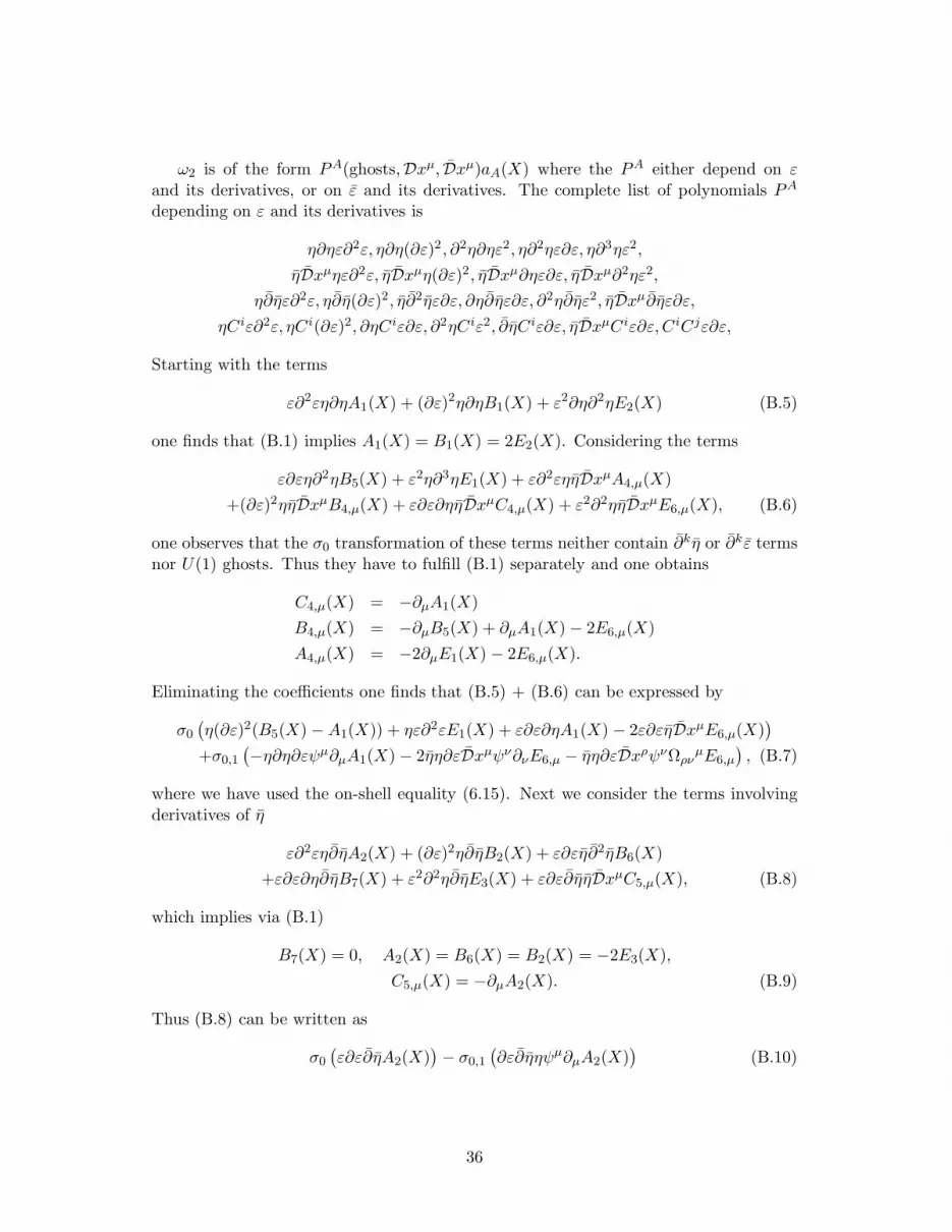
ω2 is of the form PA(ghosts,Dxµ, Dxµ)aA(X) where the PA either depend on εand its derivatives, or on ε and its derivatives. The complete list of polynomials PA

depending on ε and its derivatives is

η∂ηε∂2ε, η∂η(∂ε)2 , ∂2η∂ηε2, η∂2ηε∂ε, η∂3ηε2,

ηDxµηε∂2ε, ηDxµη(∂ε)2, ηDxµ∂ηε∂ε, ηDxµ∂2ηε2,

η∂ηε∂2ε, η∂η(∂ε)2, η∂2ηε∂ε, ∂η∂ηε∂ε, ∂2η∂ηε2, ηDxµ∂ηε∂ε,ηCiε∂2ε, ηCi(∂ε)2, ∂ηCiε∂ε, ∂2ηCiε2, ∂ηCiε∂ε, ηDxµCiε∂ε,CiCjε∂ε,

Starting with the terms

ε∂2εη∂ηA1(X) + (∂ε)2η∂ηB1(X) + ε2∂η∂2ηE2(X) (B.5)

one finds that (B.1) implies A1(X) = B1(X) = 2E2(X). Considering the terms

ε∂εη∂2ηB5(X) + ε2η∂3ηE1(X) + ε∂2εηηDxµA4,µ(X)

+(∂ε)2ηηDxµB4,µ(X) + ε∂ε∂ηηDxµC4,µ(X) + ε2∂2ηηDxµE6,µ(X), (B.6)

one observes that the σ0 transformation of these terms neither contain ∂kη or ∂kε termsnor U(1) ghosts. Thus they have to fulfill (B.1) separately and one obtains

C4,µ(X) = −∂µA1(X)

B4,µ(X) = −∂µB5(X) + ∂µA1(X) − 2E6,µ(X)

A4,µ(X) = −2∂µE1(X) − 2E6,µ(X).

Eliminating the coefficients one finds that (B.5) + (B.6) can be expressed by

σ0

(

η(∂ε)2(B5(X) −A1(X)) + ηε∂2εE1(X) + ε∂ε∂ηA1(X) − 2ε∂εηDxµE6,µ(X))

+σ0,1

(

−η∂η∂εψµ∂µA1(X) − 2ηη∂εDxµψν∂νE6,µ − ηη∂εDxρψνΩρνµE6,µ

)

, (B.7)

where we have used the on-shell equality (6.15). Next we consider the terms involvingderivatives of η

ε∂2εη∂ηA2(X) + (∂ε)2η∂ηB2(X) + ε∂εη∂2ηB6(X)

+ε∂ε∂η∂ηB7(X) + ε2∂2η∂ηE3(X) + ε∂ε∂ηηDxµC5,µ(X), (B.8)

which implies via (B.1)

B7(X) = 0, A2(X) = B6(X) = B2(X) = −2E3(X),

C5,µ(X) = −∂µA2(X). (B.9)

Thus (B.8) can be written as

σ0

(

ε∂ε∂ηA2(X))

− σ0,1

(

∂ε∂ηηψµ∂µA2(X))

(B.10)

36

and thus be removed from ω2. In the last step we consider contributions containingU(1) ghosts, i.e.

ε∂2εηCiA3,i(X) + (∂ε)2ηCiB3,i(X) + ε∂ε∂ηCiB8,i(X) + ε2∂2ηCiE4,i(X)

+ε∂ε∂ηCiB9,i(X) + ε∂εCiηDxµC6,µi(X) + ε∂εCiCjB10,ij(X). (B.11)

(B.1) imposes B10,ij(X) = B9,i(X) = B8,i(X) = 0. Furthermore we derive the condi-tions

A3,i(X) = B3,i(X) = −2E4,i(X) C6,µi(X) = −∂µA3,i(X). (B.12)

Using the on-shell equality (6.14), (B.11) can be written as

σ0

(

ε∂εCiA3,i(X))

+σ0,1

(

∂εCiηψµ∂µA3,i(X) − ∂εηηψµDxν(Ωµνi − ΩµνλGλi)A3,i(X)

)

. (B.13)

Hence, as in the case g = 3 one finds that (B.1) implies ω2 = σ0(. . . ) + σ0,1(. . . ) whichimplies (6.31) for g = 4.

C Analysis of Bianchi identities

In this appendix we summarize briefly the investigation of the Bianchi identities for two-dimensional supergravity coupled to Maxwell theory. The starting point is the structureequation

[DA,DB = −TABCDC −RABδL − FABiδi, (C.1)

where [·, · denotes the graded commutator, DA = Da,Dα contains the covariantderivatives Da and covariant supersymmetry transformations Dα, δL = (1/2)εablab isthe Lorentz generator and δi are the U(1) generators (represented trivially in our case).The “torsions” TAB

C , “curvatures” RAB and “field strengths” FABi are generically field

dependent and determined from the Bianchi identities implied by (C.1). Using theconstraints (2.5) and (2.6) one obtains for the torsions

Tαβa = 2i(γaC)αβ

Taβα = 1

4 S(γa)βα

Tabα = i

4 εab(Cγ∗)αβDβS, (C.2)

where S is the auxiliary scalar field of the gravitational multiplet. For the curvaturesone obtains

Rαβ = iS(γ∗C)αβ

Raα = i2 (γaγ∗)α

βDβS

Rab = 14 εab(S

2 + D2S), (C.3)

37

and the field strengths are given by

Fαβi = 2i(γ∗C)αβφ

i

Faαi = (γa)α

βλiβ . (C.4)

The supersymmetry transformations of λiβ and F iab turn out to be

Dαλiβ = i(γaγ∗C)αβDaφ

i + i2 (γ∗C)αβε

abF iba + i2 (γ∗C)αβSφ

i

DαFiab = −(γbDaλ

i)α + (γaDbλi)α + 1

2 εabDαSφi + 1

2 εabS(γ∗)αδλiδ. (C.5)

Introducing the corresponding connection 1-forms and proceeding along the lines of [14]one identifies the covariant derivatives Da in terms of partial derivatives and connections,and the curvatures, field strengths and torsions with two lower Lorentz indices in termsof the connections and the other field strengths. Owing to the constraint Tab

c = 0 thisyields the expression (2.2) for the spin connection. Furthermore one obtains

Fabi = Ea

nEbm(∂nA

im − ∂mA

in − (χmγnλ

i) + (χnγmλi) − 2i(χmγ∗Cχn)φ

i)

and the expression for Tabα can be used to express the supersymmetry transformation

of the auxiliary field S as

DαS = 4i(γ∗C)αβεnm∇mχn

β − i(γmC)αβχmβS.

The full BRST transformations (2.1), (2.3) and (2.4) are then obtained by adding theWeyl transformations by hand and imposing s2 = 0 on all fields. To achieve this inan off-shell setting, one introduces the super-Weyl symmetry on the gravitino and thegaugino and the local shift symmetry of the auxiliary field S.

D BRST transformations of superconformal tensor fields

This appendix collects the BRST transformations of the superconformal tensor fieldsand corresponding ghost variables derived in section 3. The transformations of the

38

undifferentiated fields read

sη = η∂η − εε

sη = η∂η − εε

sε = η∂ε− 12 ε∂η

sε = η∂ε− 12 ε∂η

sCi = ηηF i + ηελi + ηελi + εεφi

sXM = (ηD + ηD)XM + εψM + εψM

sψM = (ηD + ηD)ψM + 12 ∂ηψ

M + εDXM − εFM

sψM = (ηD + ηD)ψM + 12 ∂ηψ

M + εDXM + εFM

sFM = (ηD + ηD)FM + 12 (∂η + ∂η)FM + εDψM − εDψM

sφi = (ηD + ηD)φi + 12 (∂η + ∂η)φi + ελi + ελi

sλi = (ηD + ηD)λi + (∂η + 12 ∂η)λ

i + εDφi + εF i + ∂εφi

sλi = (ηD + ηD)λi + (12 ∂η + ∂η)λi + εDφi − εF i + ∂εφi

sF i = (ηD + ηD)F i + (∂η + ∂η)F i − εDλi + εDλi − ∂ελi + ∂ελi

The s-transformations of covariant D or D derivatives (of first or higher order) of a fieldare obtained by applying D’s and/or D’s to the transformations given above, using therules Dη = ∂η, Dη = 0, Dε = ∂ε, Dε = 0 etc, as well as [D, D] = 0. E.g., one gets

sDXM = (ηD + ηD)DXM + ∂ηDXM + εDψM + εDψM + ∂εψM

sDXM = (ηD + ηD)DXM + ∂ηDXM + εDψM + εDψM + ∂εψM

sDDXM = (ηD + ηD)DDXM + (∂η + ∂η)DDXM

+εDDψM + εDDψM + ∂εDψM + ∂εDψM

sDψM = (ηD + ηD)DψM + 32 ∂ηDψ

M + 12 ∂

2ηψM

+εD2XM + ∂εDXM − εDFM

sDψM = (ηD + ηD)DψM + 32 ∂ηDψ

M + 12 ∂

2ηψM

+εD2XM + ∂εDXM + εDFM

sDψM = (ηD + ηD)DψM + 12 ∂ηDψ

M + ∂ηDψM

+εDDXM − ∂εFM − εDFM

sDψM = (ηD + ηD)DψM + ∂ηDψM + 12 ∂ηDψ

M

+εDDXM + ∂εFM + εDFM

39

E BRST transformations of superconformal antifields

In this appendix we present the full s transformations of the superconformal antifieldsassociated with the matter and gauge multiplets, using the following notation:

GMN := H(MN)(X)

Di := Di(X)

ΩKNM := ∂KHMN(X) − ∂MHKN(X) + ∂NHKM(X)

= 2ΓKNM −HKNM (HKNM = 3∂[KHNM ])

RKLMN := ∂M∂[KHL]N(X) − ∂N∂[KHL]M(X)

= 12 (∂KΩLMN − ∂LΩKMN) = 1

2 (∂MΩKNL − ∂NΩKML).

ΩKNM and RKLMN enjoy the following properties:

ΩKMN + ΩKNM = ΩMKN + ΩNKM = 2∂KGMN

RKLMN = −RLKMN = −RKLNM , ∂[JRKL]MN = 0.

The full BRST transformations of the undifferentiated superconformal matter antifieldsare

sF ∗M = −φi∂MDi + 2GMN F

N + ψK ψNΩKNM

+(ηD + ηD)F ∗M + 1

2 (∂η + ∂η)F ∗M − εψ∗

M + εψ∗M

sψ∗M = λi∂MDi + ψN φi∂N∂MDi + 2GMN DψN

+DXNψKΩKNM − FN ψKΩMKN − ψK ψN ψLRKMLN

+(ηD + ηD)ψ∗M + (1

2 ∂η + ∂η)ψ∗M + εX∗

M + εDF ∗M + ∂εF ∗

M

sψ∗M = −λi∂MDi − ψN φi∂N∂MDi + 2GMNDψN

+DXN ψKΩNKM + FNψKΩKMN + ψKψLψNRLKMN

+(ηD + ηD)ψ∗M + (∂η + 1

2 ∂η)ψ∗M + εX∗

M − εDF ∗M − ∂εF ∗

M

sX∗M = −2GMNDDXN −DXKDXLΩKLM + FK FLΩMKL

+DψKψLΩMLK − ψKDψLΩKML

+DXN ψK ψLRNMLK + DXNψKψLRLKNM

+FNψK ψL∂MΩKLN + 12 ψ

RψK ψN ψL∂MRKRLN

+F i∂MDi − (ψN λi − ψNλi + FN φi + ψN ψK φi∂K)∂N∂MDi

+(ηD + ηD)X∗M + (∂η + ∂η)X∗

M

+εDψ∗M + εDψ∗

M + ∂εψ∗M + ∂εψ∗

M

40

The s transformation of the superconformal antifields for the gauge multiplet read

sλ∗i = ψM∂MDi

+(ηD + ηD)λ∗i + 12 ∂ηλ

∗i + εφ∗i − εA∗

i

sλ∗i = −ψM∂MDi

+(ηD + ηD)λ∗i + 12 ∂ηλ

∗i + εφ∗i − εA∗

i

sφ∗i = −FM∂MDi − ψM ψN∂N∂MDi

+(ηD + ηD)φ∗i + 12 (∂η + ∂η)φ∗i

+εDλ∗i + εDλ∗i − εεC∗i

sA∗i = −DXM∂MDi

+(ηD + ηD)A∗i + ∂ηA∗

i

+εDλ∗i − εDλ∗i − ∂ελ∗i − εεC∗i

sA∗i = DXM∂MDi

+(ηD + ηD)A∗i + ∂ηA∗

i

+εDλ∗i − εDλ∗i − ∂ελ∗i − εεC∗i

sC∗i = −DA∗

i − DA∗i + (ηD + ηD)C∗

i + (∂η + ∂η)C∗i

The BRST transformations of covariant derivatives of the covariant antifields (suchas sDX∗

M) are obtained from the above formulae by means of the rules described inappendix D.

41

References

[1] P. Ramond, “Dual Theory For Free Fermions,” Phys. Rev. D 3 (1971) 2415-2418.

[2] A. Neveu and J. H. Schwarz, “Factorizable Dual Model Of Pions,” Nucl. Phys. B31 (1971) 86-112.

[3] A. Neveu and J. H. Schwarz, “Quark Model Of Dual Pions,” Phys. Rev. D 4 (1971)1109-1111.

[4] S. Deser and B. Zumino, “A Complete Action For The Spinning String,” Phys.Lett. B 65 (1976) 369-373.

[5] L. Brink, P. Di Vecchia and P. Howe, “A Locally Supersymmetric AndReparametrization Invariant Action For The Spinning String,” Phys. Lett. B 65

(1976) 471-474.

[6] F. Brandt, A. Kling and M. Kreuzer, “Actions and symmetries of NSR superstringsand D-strings,” Phys. Lett. B 494 (2000) 155-160 [hep-th/0006152].

[7] E. Bergshoeff, S. Randjbar-Daemi, A. Salam, H. Sarmadi and E. Sezgin, “LocallySupersymmetric Sigma Model With Wess-Zumino Term In Two-Dimensions AndCritical Dimensions For Strings,” Nucl. Phys. B 269 (1986) 77-96.

[8] F. Brandt, J. Gomis and J. Simon, “The rigid symmetries of bosonic D-strings,”Phys. Lett. B 419 (1998) 148-156 [hep-th/9707063].

[9] F. Brandt, J. Gomis and J. Simon, “Cohomological analysis of bosonic D-stringsand 2d sigma models coupled to abelian gauge fields,” Nucl. Phys. B 523 (1998)623-662 [hep-th/9712125].

[10] G. Barnich, F. Brandt and M. Henneaux, “Local BRST cohomology in gauge the-ories,” Phys. Rept. 338 (2000) 439-569 [hep-th/0002245].

[11] G. Barnich, F. Brandt and M. Henneaux, “Local BRST cohomology in EinsteinYang-Mills theory,” Nucl. Phys. B 455 (1995) 357-408 [hep-th/9505173].

[12] F. Brandt, N. Dragon and M. Kreuzer, “The Gravitational Anomalies,” Nucl. Phys.B 340 (1990) 187-224.

[13] N. Dragon, “BRS Symmetry and Cohomology,” hep-th/9602163.

[14] F. Brandt, “Local BRST Cohomology and Covariance,” Commun. Math. Phys. 190(1997) 459-489 [hep-th/9604025].

[15] G. Barnich, F. Brandt and M. Henneaux, “Local BRST cohomology in the antifieldformalism: I. General theorems,” Commun. Math. Phys. 174 (1995) 57-91 [hep-th/9405109].

[16] G. Barnich and M. Henneaux, “Consistent couplings between fields with a gaugefreedom and deformations of the master equation,” Phys. Lett. B311 (1993) 123-129 [hep-th/9304057].

42

[17] F. Brandt, W. Troost and A. Van Proeyen, “Background charges and consistentcontinuous deformations of 2d gravity theories,” Phys. Lett. B 374 (1996) 31-36[hep-th/9510195].

[18] O. Piguet and S. P. Sorella, “Algebraic renormalization: Perturbative renormal-ization, symmetries and anomalies,” Berlin, Germany: Springer (1995) 134 p.(Lecture notes in physics: m28)).

[19] F. Brandt, W. Troost and A. Van Proeyen, “The BRST–antibracket cohomology of2d gravity conformally coupled to scalar matter,” Nucl. Phys. B 464 (1996) 353-408[hep-th/9509035].

[20] F. Brandt, J. Gomis and J. Simon, “D-string on near horizon geometries and infiniteconformal symmetry,” Phys. Rev. Lett. 81 (1998) 1770-1773 [hep-th/9803196].

[21] L. Alvarez-Gaume and D. Z. Freedman, “Geometrical Structure And UltravioletFiniteness In The Supersymmetric Sigma Model,” Commun. Math. Phys. 80 (1981)443-451.

[22] S. J. Gates, C. M. Hull and M. Rocek, “Twisted Multiplets And New Supersym-metric Nonlinear Sigma Models,” Nucl. Phys. B 248 (1984) 157-186.

[23] C. M. Hull and E. Witten, “Supersymmetric Sigma Models And The HeteroticString,” Phys. Lett. B 160 (1985) 398-402.

[24] A. Kling, “BRST cohomology of Dirichlet-Superstrings”, diploma thesis, Vienna1998 (unpublished).

[25] P. S. Howe, “Super Weyl Transformations In Two-Dimensions”, J. Phys. A 12

(1979) 393-402.

[26] F. Brandt, “Gauge covariant algebras and local BRST cohomology,” Contemp.Math. 219 (1999) 53-67 [hep-th/9711171].

[27] F. Brandt, “Jet coordinates for local BRST cohomology,” Lett. Math. Phys. (toappear) [math-ph/0103006].

[28] F. Delduc and F. Gieres, “Beltrami differentials, conformal models and their su-persymmetric generalizations”, Class. Quant. Grav. 7 (1990) 1907-1952.

[29] R. Grimm, “Left-Right Decomposition of Two-Dimensional Superspace Geometryand Its BRS Structure”, Ann. Phys. 200 (1990) 49-100.

[30] I. A. Batalin and G. A. Vilkovisky, “Quantization Of Gauge Theories With LinearlyDependent Generators”, Phys. Rev. D 28 (1983) 2567-2582

[31] I. A. Batalin and G. A. Vilkovisky, “Gauge Algebra And Quantization”, Phys. Lett.B 102 (1981) 27-31.

[32] M. Henneaux and C. Teitelboim, “Quantization of Gauge Systems”, Princeton Uni-versity Press, Princeton, 1992.

[33] J. Gomis, J. Parıs and S. Samuel, “Antibracket, antifields and gauge theory quan-tization” Phys. Rept. 259 (1995) 1-145 [hep-th/9412228].

43