HAL Id: hal-00618167https://hal.archives-ouvertes.fr/hal-00618167v8

Preprint submitted on 26 Sep 2013

HAL is a multi-disciplinary open accessarchive for the deposit and dissemination of sci-entific research documents, whether they are pub-lished or not. The documents may come fromteaching and research institutions in France orabroad, or from public or private research centers.

L’archive ouverte pluridisciplinaire HAL, estdestinée au dépôt et à la diffusion de documentsscientifiques de niveau recherche, publiés ou non,émanant des établissements d’enseignement et derecherche français ou étrangers, des laboratoirespublics ou privés.

Accessing the cohomology of discrete groups above theirvirtual cohomological dimension

Alexander D. Rahm

To cite this version:Alexander D. Rahm. Accessing the cohomology of discrete groups above their virtual cohomologicaldimension. 2013. �hal-00618167v8�

ACCESSING THE COHOMOLOGY OF DISCRETE GROUPS

ABOVE THEIR VIRTUAL COHOMOLOGICAL DIMENSION

ALEXANDER D. RAHM

Abstract. We introduce a method to explicitly determine the Farrell–Tate cohomology ofdiscrete groups. We apply this method to the Coxeter triangle and tetrahedral groups as well asto the Bianchi groups, i.e. PSL2(O) for O the ring of integers in an imaginary quadratic numberfield, and to their finite index subgroups. We show that the Farrell–Tate cohomology of theBianchi groups is completely determined by the numbers of conjugacy classes of finite subgroups.In fact, our access to Farrell–Tate cohomology allows us to detach the information about itfrom geometric models for the Bianchi groups and to express it only with the group structure.Formulae for the numbers of conjugacy classes of finite subgroups have been determined in athesis of Kramer, in terms of elementary number-theoretic information on O. An evaluation ofthese formulae for a large number of Bianchi groups is provided numerically in the appendix.Our new insights about their homological torsion allow us to give a conceptual description ofthe cohomology ring structure of the Bianchi groups.

1. Introduction

Our objects of study are discrete groups Γ such that Γ admits a torsion-free subgroup offinite index. By a theorem of Serre, all the torsion-free subgroups of finite index in Γ havethe same cohomological dimension; this dimension is called the virtual cohomological dimension(abbreviated vcd) of Γ. Above the vcd, the (co)homology of a discrete group is determined by itssystem of finite subgroups. We are going to discuss it in terms of Farrell–Tate cohomology (which

we will by now just call Farrell cohomology). The Farrell cohomology Hqis identical to group

cohomology Hq in all degrees q above the vcd, and extends in lower degrees to a cohomologytheory of the system of finite subgroups. Details are elaborated in [8, chapter X]. So for instanceconsidering the Coxeter groups, the virtual cohomological dimension of all of which vanishes,their Farrell cohomology is identical to all of their group cohomology. In Section 2, we willintroduce a method of how to explicitly determine the Farrell cohomology : By reducing torsionsub-complexes. This method has also been implemented on the computer [11], which allows usto check the results that we obtain by our arguments. We apply our method to the Coxetertriangle and tetrahedral groups in Section 3, and to the Bianchi groups in Sections 4 through 6.

In detail, we require any discrete group Γ under our study to be provided with a cell complexon which it acts cellularly. We call this a Γ–cell complex. Let X be a Γ–cell complex; and let ℓ bea prime number. Denote by X(ℓ) the set of all the cells σ of X, such that there exists an elementof order ℓ in the stabilizer of the cell σ. In the case that the stabilizers are finite and fix theircells point-wise, the set X(ℓ) is a Γ–sub-complex of X, and we call it the ℓ–torsion sub-complex.

Date: September 26, 2013.2010 Mathematics Subject Classification. 11F75, Cohomology of arithmetic groups.Funded by the Irish Research Council for Science, Engineering and Technology.

1

2 RAHM

For the Coxeter tetrahedral groups, generated by the reflections on the sides of a tetrahedronin hyperbolic 3-space, we obtain the following. Denote by Dℓ the dihedral group of order 2ℓ.

Corollary 1 (Corollary to Theorem 12.). Let Γ be a Coxeter tetrahedral group, and ℓ > 2 be aprime number. Then there is an isomorphism Hq(Γ; Z/ℓ) ∼= (Hq(Dℓ; Z/ℓ))

m, with m the numberof connected components of the orbit space of the ℓ–torsion sub-complex of the Davis complexof Γ.

We specify the exponent m in the tables in Figures 3 through 2.Some individual procedures of our method have already been applied as ad hoc tricks by

experts since [29], usually without providing a printed explanation of the tricks. An essentialadvantage of establishing a systematic method rather than using a set of ad hoc tricks, is thatwe can find ways to compute directly the quotient of the reduced torsion sub-complexes, workingoutside of the geometric model and skipping the often very laborious calculation of the orbitspace of the Γ–cell complex. This provides access to the cohomology of many discrete groupsfor which the latter orbit space calculation is far out of reach. For the Bianchi groups, we givein Section 4 an instance of how to construct the quotient of the reduced torsion sub-complexoutside of the geometric model.

Results for the Bianchi groups. Denote by Q(√−m), with m a square-free positive integer,

an imaginary quadratic number field, and by O−m its ring of integers. The Bianchi groups arethe groups PSL2(O−m). The Bianchi groups may be considered as a key to the study of a largerclass of groups, the Kleinian groups, which date back to work of Henri Poincare [20]. In fact,each non-co-compact arithmetic Kleinian group is commensurable with some Bianchi group [18].A wealth of information on the Bianchi groups can be found in the monographs [13], [12], [18].Kramer [17] has determined number-theoretic formulae for the numbers of conjugacy classes offinite subgroups in the Bianchi groups, using numbers of ideal classes in orders of cyclotomicextensions of Q(

√−m).In Section 5, we express the homological torsion of the Bianchi groups as a function of these

numbers of conjugacy classes. To achieve this, we build on the geometric techniques of [22],which depend on the explicit knowledge of the quotient space of geometric models for the Bianchigroups — like any technique effectively accessing the (co)homology of the Bianchi groups, eitherdirectly [27], [32] or via a group presentation [5]. For the Bianchi groups, we can in Sections 4and 5 detach invariants of the group actions from the geometric models, in order to express themonly by the group structure itself, in terms of conjugacy classes of finite subgroups, normalizersof the latter, and their interactions. This information is already contained in our reduced torsionsub-complexes.

Not only does this provide us with exact formulae for the homological torsion of the Bianchigroups, the power of which we can see in the numerical evaluations of Appendices A.1 and A.2,also it allows us to understand the role of the centralizers of the finite subgroups — and this ishow in [21], some more fruits of the present results are harvested (in terms of the Chen/Ruanorbifold cohomology of the orbifolds given by the action of the Bianchi groups on complexifiedhyperbolic space).

Except for the Gaussian and Eisenstein integers, which can easily be treated separately [27],[22], all the rings of integers of imaginary quadratic number fields admit as only units {±1}.In the latter case, we call PSL2(O) a Bianchi group with units {±1}. For the possible types offinite subgroups in the Bianchi groups, see Lemma 18 : There are five non-trivial possibilities.

ACCESSING THE COHOMOLOGY OF DISCRETE GROUPS ABOVE THEIR VCD 3

In Theorem 2, the proof of which we give in Section 5, we give a formula expressing preciselyhow the Farrell cohomology of the Bianchi groups with units {±1} depends on the numbers ofconjugacy classes of non-trivial finite subgroups of the occurring five types. The main step inorder to prove this, is to read off the Farrell cohomology from the quotient of the reduced torsionsub-complexes.

Kramer’s formulae express the numbers of conjugacy classes of the five types of non-trivialfinite subgroups in the Bianchi groups, where the symbols in the first row are Kramer’s notationsfor the number of their conjugacy classes:

λ4 λ6 µ2 µ3 µT

Z/2 Z/3 D2 D3 A4

We are going to use these symbols also for the numbers of conjugacy classes in Γ, where Γ is afinite index subgroup in a Bianchi group. Recall that for ℓ = 2 and ℓ = 3, we can express thethe dimensions of the homology of Γ with coefficients in the field Fℓ with ℓ elements in degreesabove the virtual cohomological dimension of the Bianchi groups – which is 2 – by the Poincareseries

P ℓΓ(t) :=

∞∑

q > 2

dimFℓHq (Γ; Fℓ) t

q,

which has been suggested by Grunewald. Further let P b (t) := −2t3

t−1 , which equals the series

P 2Γ(t) of the groups Γ the quotient of the reduced 2–torsion sub-complex of which is a circle.

Denote by

• P ∗D2

(t) := −t3(3t−5)2(t−1)2

, the Poincare series over dimF2 Hq (D2; F2)− 32 dimF2 Hq (Z/2; F2)

• and by P ∗A4

(t) := −t3(t3−2t2+2t−3)2(t−1)2(t2+t+1)

, the Poincare series over

dimF2 Hq (A4; F2)−1

2dimF2 Hq (Z/2; F2) .

In 3-torsion, let Pb b

(t) := −t3(t2−t+2)(t−1)(t2+1)

, which equals the series P 3Γ(t) for the Bianchi groups the

quotient of the reduced 3–torsion sub-complex of which is a single edge without identifications.

Theorem 2. For any finite index subgroup Γ in a Bianchi group with units {±1}, the grouphomology in degrees above its virtual cohomological dimension is given by the Poincare series

P 2Γ(t) =

(λ4 −

3µ2 − 2µT

2

)P b (t) + (µ2 − µT )P

∗D2

(t) + µTP∗A4

(t)

and

P 3Γ(t) =

(λ6 −

µ3

2

)P b (t) +

µ3

2P

b b(t).

Our method is further applied in [6] to obtain also the Farrell cohomology of SL2 (O−m).

Organization of the paper. In Section 2, we introduce our method to explicitly determineFarrell cohomology: By reducing the torsion sub-complexes. We apply our method to theCoxeter triangle and tetrahedral groups in Section 3. In Section 4, we show how to read off theFarrell cohomology of the Bianchi groups from the reduced torsion sub-complexes. We achievethis by showing that for the Bianchi groups, the quotients of the reduced torsion sub-complexesare homeomorphic to conjugacy classes graphs that we can define without reference to any

4 RAHM

geometric model. This enables us in Section 5 to prove the formulae for the homological torsionof the Bianchi groups in terms of numbers of conjugacy classes of finite subgroups. We use thisto establish the structure of the classical cohomology rings of the Bianchi groups in Section 6.Kramer has given number-theoretic formulae for these numbers of conjugacy classes, and weevaluate them numerically in Appendices A.1 and A.2. Finally, we present some numericalasymptotics on the numbers of conjugacy classes in Appendix A.3.

Acknowledgements. The author is indebted to the late great mathematician Fritz Grunewald,for telling him about the existence and providing him a copy of Kramer’s Diplom thesis. Warmestthanks go to Ruben Sanchez-Garcıa for providing his implementation of the Davis complex, toMike Davis and Gotz Pfeiffer for discussions on the Coxeter groups, to Oliver Braunling for acorrespondence on the occurrence of given norms on rings of integers, to Nicolas Bergeron fordiscussions on asymptotics, to Philippe Elbaz-Vincent and Matthias Wendt for a very carefullecture of the manuscript and helpful suggestions, and to Graham Ellis and Stephen S. Gelbartfor support and encouragement.

2. Reduction of torsion sub-complexes

LetX be a finite-dimensional cell complex with a cellular action of a discrete group Γ, such thateach cell stabilizer fixes its cell point-wise. Let ℓ be a prime such that every non-trivial finite ℓ–subgroup of Γ admits a contractible fixed point set. We keep these requirements on the Γ–actionas a general assumption throughout this article. Then, the Γ–equivariant Farrell cohomology

of X, for any trivial Γ–module M of coefficients, gives us the ℓ–primary part H∗(Γ; M)(ℓ) of the

Farrell cohomology of Γ, as follows.

Proposition 3 (Brown [8]). Under our general assumption, the canonical map

H∗(Γ; M)(ℓ) → H

∗

Γ(X; M)(ℓ)

is an isomorphism.

The classical choice [8] is to take for X the geometric realization of the partially orderedset of non-trivial finite subgroups (respectively, non-trivial elementary Abelian ℓ–subgroups)of Γ, the latter acting by conjugation. The stabilizers are then the normalizers, which in manydiscrete groups are infinite. And it can impose great computational challenges to determine a

group presentation for them. When we want to compute the module H∗

Γ(X; M)(ℓ) subject toProposition 3, at least we must get to know the (ℓ–primary part of the) Farrell cohomologyof these normalizers. The Bianchi groups are an instance that different isomorphism types canoccur for this cohomology at different conjugacy classes of elementary Abelian ℓ–subgroups, bothfor ℓ = 2 and ℓ = 3. As the only non-trivial elementary Abelian 3–subgroups in the Bianchigroups are of rank 1, the orbit space Γ\X consists only of one point for each conjugacy class oftype Z/3 and a corollary [8] from Proposition 3 decomposes the 3–primary part of the Farrellcohomology of the Bianchi groups into the direct product over their normalizers. However, dueto the different possible homological types of the normalizers (in fact, two of them occur), thefinal result remains unclear and subject to tedious case-by-case computations of the normalizers.

In contrast, in the cell complex we are going to develop, the connected components of the orbitspace are for the 3–torsion in the Bianchi groups not simple points, but have either the shapeb b or b . This dichotomy already contains the information about the occurring normalizer.

ACCESSING THE COHOMOLOGY OF DISCRETE GROUPS ABOVE THEIR VCD 5

Definition 4. Let ℓ be a prime number. The ℓ–torsion sub-complex of the Γ–cell complex Xconsists of all the cells of X the stabilizers in Γ of which contain elements of order ℓ.

We are from now on going to require the cell complex X to admit only finite stabilizers in Γ,and we require the action of Γ on the coefficient module M to be trivial. Then obviously only

cells from the ℓ–torsion sub-complex contribute to H∗

Γ(X; M)(ℓ). We are going to reduce theℓ–torsion sub-complex to one which still carries the Γ–equivariant Farrell cohomology of X, butcan have considerably less orbits of cells, can be easier to handle in practice, and, for certainclasses of groups, leads us to an explicit structural description of the Farrell cohomology of Γ.The pivotal property of this reduced ℓ–torsion sub-complex will be given in Theorem 7.

Condition A. In the ℓ–torsion sub-complex, let σ be a cell of dimension n − 1, lying in theboundary of precisely two n–cells τ1 and τ2, the latter cells representing two different orbits.Assume further that no higher-dimensional cells of the ℓ–torsion sub-complex touch σ; and thatthe n–cell stabilizers admit an isomorphism Γτ1

∼= Γτ2 .

Where this condition is fulfilled in the ℓ–torsion sub-complex, we merge the cells τ1 andτ2 along σ and do so for their entire orbits, if and only if they meet the following additionalcondition. We never merge two cells the interior of which contains two points on the same orbit.Let ℓ be a prime number, and denote by mod ℓ homology group homology with Z/ℓ–coefficientsunder the trivial action.

Condition B. The inclusion Γτ1 ⊂ Γσ induces an isomorphism on mod ℓ homology.

Lemma 5. Let X(ℓ) be the Γ–complex obtained by orbit-wise merging two n–cells of the ℓ–torsionsub-complex X(ℓ) which satisfy Conditions A and B. Then,

H∗

Γ(X(ℓ); M)(ℓ) ∼= H∗

Γ(X(ℓ); M)(ℓ).

Proof of Lemma 5. Consider the equivariant spectral sequence in Farrell cohomology [8]. Onthe ℓ–torsion sub-complex, it includes a map

H∗(Γσ; M)(ℓ)

d(n−1),∗1 |

H∗(Γσ ;M)(ℓ)

// H∗(Γτ1 ; M)(ℓ) ⊕ H

∗(Γτ2 ; M)(ℓ) ,

which is the diagonal map with blocks the isomorphisms H∗(Γσ; M)(ℓ)

∼=// H

∗(Γτi ; M)(ℓ) ,

induced by the inclusions Γτi → Γσ. The latter inclusions are required to induce isomorphismsin Condition B. If for the orbit of τ1 or τ2 we have chosen a representative which is not adjacentto σ, then this isomorphism is composed with the isomorphism induced by conjugation with

the element of Γ carrying the cell to one adjacent to σ. Hence, the map d(n−1),∗1 |

H∗

(Γσ ;M)(ℓ)

has vanishing kernel, and dividing its image out of H∗(Γτ1 ; M)(ℓ) ⊕ H

∗(Γτ2 ; M)(ℓ) gives us the

ℓ–primary part H∗(Γτ1∪τ2 ; M)(ℓ) of the Farrell cohomology of the union τ1∪τ2 of the two n–cells,

once that we make use of the isomorphism Γτ1∼= Γτ2 of Condition A. As by Condition A no

higher-dimensional cells are touching σ, there are no higher degree differentials interfering. �

By a “terminal vertex”, we will denote a vertex with no adjacent higher-dimensional cells andprecisely one adjacent edge in the quotient space, and by “cutting off” the latter edge, we willmean that we remove the edge together with the terminal vertex from our cell complex.

6 RAHM

Definition 6. The reduced ℓ–torsion sub-complex associated to a Γ–cell complexX which fulfillsour general assumption, is the cell complex obtained by recursively merging orbit-wise all thepairs of cells satisfying Conditions A and B; and cutting off edges that admit a terminal vertextogether with which they satisfy Condition B.

Theorem 7. There is an isomorphism between the ℓ–primary parts of the Farrell cohomologyof Γ and the Γ–equivariant Farrell cohomology of the reduced ℓ–torsion sub-complex.

Proof. We apply Proposition 3 to the cell complex X, and then we apply Lemma 5 each timethat we orbit-wise merge a pair of cells of the ℓ–torsion sub-complex, or that we cut off anedge. �

In order to have a practical criterion for checking Condition B, we make use of the followingstronger condition.

Here, we write NΓσ for taking the normalizer in Γσ and Sylowℓ for picking an arbitrarySylow ℓ–subgroup. This is well defined because all Sylow ℓ–subgroups are conjugate. We useZassenhaus’s notion for a finite group to be ℓ–normal, if the center of one of its Sylow ℓ–subgroupsis the center of every Sylow ℓ–subgroup in which it is contained.

Condition B’. The group Γσ admits a (possibly trivial) normal subgroup Tσ with trivial mod ℓhomology and with quotient group Gσ; and the group Γτ1 admits a (possibly trivial) normalsubgroup Tτ with trivial mod ℓ homology and with quotient group Gτ making the sequences

1 → Tσ → Γσ → Gσ → 1 and 1 → Tτ → Γτ1 → Gτ → 1

exact and satisfying one of the following.

(1) Either Gτ∼= Gσ , or

(2) Gσ is ℓ–normal and Gτ∼= NGσ(center(Sylowℓ(Gσ))), or

(3) both Gσ and Gτ are ℓ–normal and there is a (possibly trivial) group T with trivial mod ℓhomology making the sequence

1 → T → NGσ(center(Sylowℓ(Gσ))) → NGτ (center(Sylowℓ(Gτ ))) → 1

exact.

Lemma 8. Condition B’ implies Condition B.

For the proof of ( B’(2) ⇒ B), we use Swan’s extension [31, final corollary] to Farrell coho-mology of the Second Theorem of Grun [14, Satz 5].

Theorem 9 (Swan). Let G be a ℓ–normal finite group, and let N be the normalizer of the centerof a Sylow ℓ–subgroup of G. Let M be any trivial G–module. Then the inclusion and transfer

maps both are isomorphisms between the ℓ–primary components of H∗(G; M) and H

∗(N ; M).

For the proof of ( B’(3) ⇒ B), we make use of the following direct consequence of the Lyndon–Hochschild–Serre spectral sequence.

Lemma 10. Let T be a group with trivial mod ℓ homology, and consider any group extension

1 → T → E → Q → 1.

Then the map E → Q induces an isomorphism on mod ℓ homology.

ACCESSING THE COHOMOLOGY OF DISCRETE GROUPS ABOVE THEIR VCD 7

This statement may look like a triviality, but it becomes wrong as soon as we exchange theroles of T and Q in the group extension. In degrees 1 and 2, our claim follows from [8, VII.(6.4)].In arbitrary degree, it is more or less known and we can proceed through the following easy steps.

Proof. Consider the Lyndon–Hochschild–Serre spectral sequence associated to the group exten-sion, namely

E2p,q = Hp(Q; Hq(T ; Z/ℓ)) converges to Hp+q(E; Z/ℓ).

By our assumption, Hq(T ; Z/ℓ) is trivial, so this spectral sequence concentrates in the row q = 0,degenerates on the second page and yields isomorphisms

(1) Hp(Q; H0(T ; Z/ℓ)) ∼= Hp(E; Z/ℓ).

As for the modules of co-invariants, we have ((Z/ℓ)T )Q∼= (Z/ℓ)E [19], the trivial actions of

E and T induce that also the action of Q on the coefficients in H0(T ; Z/ℓ) is trivial. Thus,Isomorphism (1) becomes Hp(Q; Z/ℓ) ∼= Hp(E; Z/ℓ). �

The above lemma directly implies that any extension of two groups both having trivial mod ℓhomology, again has trivial mod ℓ homology.

Proof of Lemma 8. We combine Theorem 9 and Lemma 10 in the obvious way. �

Remark 11. The computer implementation [11] checks Conditions B′(1) and B′(2) for eachpair of cell stabilizers, using a presentation of the latter in terms of matrices, permutationcycles or generators and relators. In the below examples however, we do avoid this case-by-casecomputation by a general determination of the isomorphism types of pairs of cell stabilizers forwhich group inclusion induces an isomorphism on mod ℓ homology. The latter method is to beconsidered as the procedure of preference, because it allows us to deduce statements that holdfor the whole class of concerned groups.

3. Farrell cohomology of the Coxeter tetrahedral groups

Figure 1. Quotient of theDavis complex for a trian-gle group (diagram reprintedwith the kind permission ofSanchez-Garcia [26]).

Recall that a Coxeter group is a group admitting a presentation

〈g1, g2, ..., gn | (gigj)mi,j = 1〉,

where mi,i = 1; for i 6= j we have mi,j > 2; and mi,j = ∞ ispermitted, meaning that (gigj) is not of finite order. As the Coxetergroups admit a contractible classifying space for proper actions [10],their Farrell cohomology yields all of their group cohomology. So inthis section, we make use of this fact to determine the latter. Forfacts about Coxeter groups, and especially for the Davis complex,we refer to [10]. Recall that the simplest example of a Coxetergroup, the dihedral group Dn, is an extension

1 → Z/ℓ → Dn → Z/2 → 1,

8 RAHM

so we can make use of the original application [33] of Wall’s lemmato obtain its mod ℓ homology for prime numbers ℓ > 2,

Hq(Dn; Z/ℓ) ∼=

Z/ℓ, q = 0,

Z/gcd(n, ℓ), q ≡ 3 or 4 mod 4,

0, otherwise.

Theorem 12. Let ℓ > 2 be a prime number. Let Γ be a Coxeter group admitting a Coxetersystem with at most four generators, and relator orders not divisible by ℓ2. Let Z(ℓ) be theℓ–torsion sub-complex of the Davis complex of Γ. If Z(ℓ) is at most one-dimensional and itsorbit space contains no loop nor bifurcation, then the mod ℓ homology of Γ is isomorphic to(Hq(Dℓ; Z/ℓ))

m, with m the number of connected components of the orbit space of Z(ℓ).

The conditions of this theorem are for instance fulfilled by the Coxeter tetrahedral groups;we specify the exponent m for them in the tables in Figures 3 through 2. In order to proveTheorem 12, we lean on the following technical lemma. When a group G contains a Coxetergroup H properly (i.e. H 6= G) as a subgroup, then we call H a Coxeter subgroup of G.

Lemma 13. Let ℓ > 2 be a prime number; and let Γσ be a finite Coxeter group with n 6 4generators. If Γσ is not a direct product of two dihedral groups and not associated to the Coxeterdiagram F4 or H4, then Condition B′ is fulfilled for the triple consisting of ℓ, the group Γσ andany of its Coxeter subgroups Γτ1 with (n− 1) generators that contains ℓ–torsion elements.

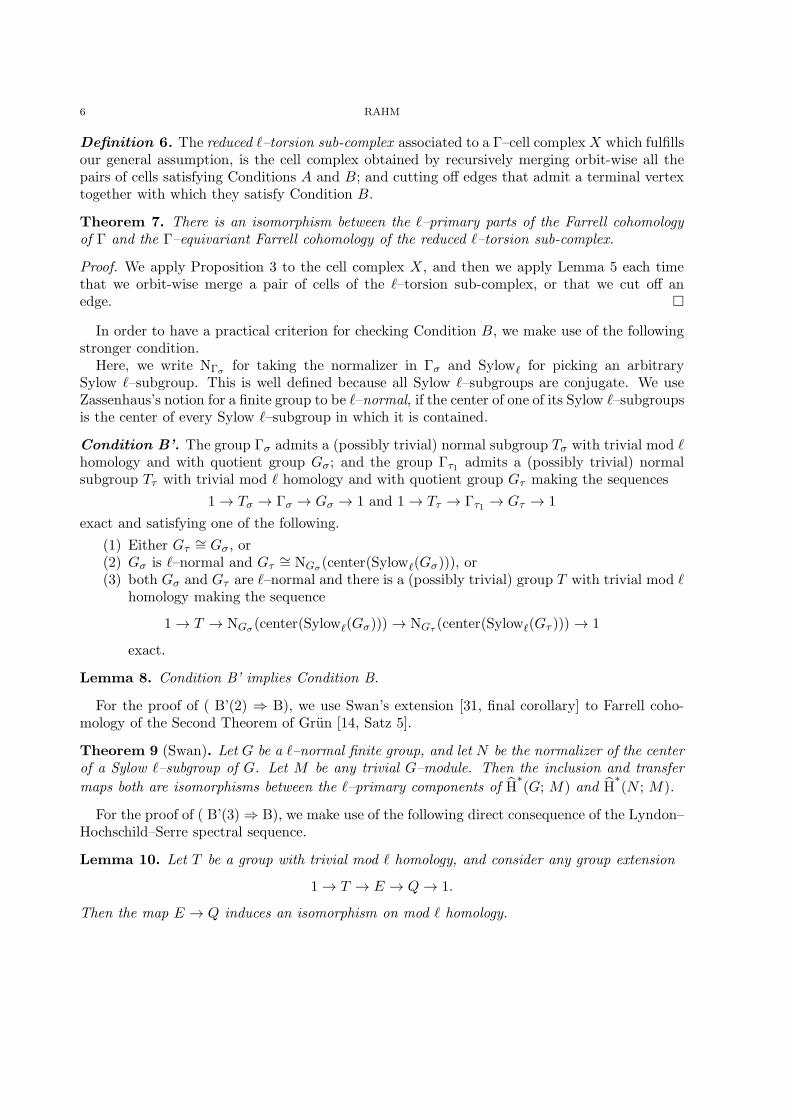
Proof. The dihedral groups admit only Coxeter subgroups with two elements, so without ℓ–torsion. There are only finitely many other isomorphism types of irreducible finite Coxetergroups with at most four generators, specified by the Coxeter diagrams

A1 A3 A4 B3 B4 D4 H3

• b b b b b b b b 4 b b b b b4 b

b

b

b bb 5 b b

on which we can check the condition case by case.

A1. The symmetric group S2 admits no Coxeter subgroups.A3. The symmetric group S4 is 3–normal; and its Sylow-3–subgroups are of type Z/3, so they

are identical to their center. Their normalizers in S4 match the Coxeter subgroups oftype D3 that one obtains by omitting one of the generators of S4 at an end of its Coxeterdiagram. The other possible Coxeter subgroup type is (Z/2)2, obtained by omitting themiddle generator in this diagram, and contains no 3–torsion.

A4. The Coxeter subgroups with three generators in the symmetric group S5 are D3 × Z/2and S4, so we only need to consider 3–torsion. The group S5 is 3–normal; the nor-malizer of the center of any of its Sylow-3–subgroups is of type D3 × Z/2. So for theCoxeter subgroup S4, we use the normalizer D3 of its Sylow-3–subgroup Z/3; and seethat Condition B′(3) is fulfilled.

B3. We apply Lemma 10 to the Coxeter group (Z/2)3 ⋊ D3, and retain only D3, which isisomorphic to the only Coxeter subgroup admitting 3–torsion.

ACCESSING THE COHOMOLOGY OF DISCRETE GROUPS ABOVE THEIR VCD 9

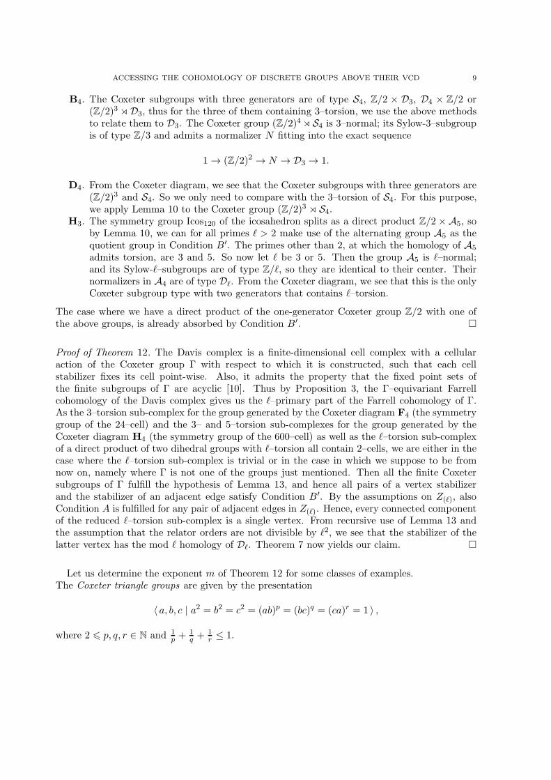
B4. The Coxeter subgroups with three generators are of type S4, Z/2 × D3, D4 × Z/2 or(Z/2)3 ⋊D3, thus for the three of them containing 3–torsion, we use the above methodsto relate them to D3. The Coxeter group (Z/2)4 ⋊S4 is 3–normal; its Sylow-3–subgroupis of type Z/3 and admits a normalizer N fitting into the exact sequence

1 → (Z/2)2 → N → D3 → 1.

D4. From the Coxeter diagram, we see that the Coxeter subgroups with three generators are(Z/2)3 and S4. So we only need to compare with the 3–torsion of S4. For this purpose,we apply Lemma 10 to the Coxeter group (Z/2)3 ⋊ S4.

H3. The symmetry group Icos120 of the icosahedron splits as a direct product Z/2 ×A5, soby Lemma 10, we can for all primes ℓ > 2 make use of the alternating group A5 as thequotient group in Condition B′. The primes other than 2, at which the homology of A5

admits torsion, are 3 and 5. So now let ℓ be 3 or 5. Then the group A5 is ℓ–normal;and its Sylow-ℓ–subgroups are of type Z/ℓ, so they are identical to their center. Theirnormalizers in A4 are of type Dℓ. From the Coxeter diagram, we see that this is the onlyCoxeter subgroup type with two generators that contains ℓ–torsion.

The case where we have a direct product of the one-generator Coxeter group Z/2 with one ofthe above groups, is already absorbed by Condition B′. �

Proof of Theorem 12. The Davis complex is a finite-dimensional cell complex with a cellularaction of the Coxeter group Γ with respect to which it is constructed, such that each cellstabilizer fixes its cell point-wise. Also, it admits the property that the fixed point sets ofthe finite subgroups of Γ are acyclic [10]. Thus by Proposition 3, the Γ–equivariant Farrellcohomology of the Davis complex gives us the ℓ–primary part of the Farrell cohomology of Γ.As the 3–torsion sub-complex for the group generated by the Coxeter diagram F4 (the symmetrygroup of the 24–cell) and the 3– and 5–torsion sub-complexes for the group generated by theCoxeter diagram H4 (the symmetry group of the 600–cell) as well as the ℓ–torsion sub-complexof a direct product of two dihedral groups with ℓ–torsion all contain 2–cells, we are either in thecase where the ℓ–torsion sub-complex is trivial or in the case in which we suppose to be fromnow on, namely where Γ is not one of the groups just mentioned. Then all the finite Coxetersubgroups of Γ fulfill the hypothesis of Lemma 13, and hence all pairs of a vertex stabilizerand the stabilizer of an adjacent edge satisfy Condition B′. By the assumptions on Z(ℓ), alsoCondition A is fulfilled for any pair of adjacent edges in Z(ℓ). Hence, every connected componentof the reduced ℓ–torsion sub-complex is a single vertex. From recursive use of Lemma 13 andthe assumption that the relator orders are not divisible by ℓ2, we see that the stabilizer of thelatter vertex has the mod ℓ homology of Dℓ. Theorem 7 now yields our claim. �

Let us determine the exponent m of Theorem 12 for some classes of examples.The Coxeter triangle groups are given by the presentation

〈 a, b, c | a2 = b2 = c2 = (ab)p = (bc)q = (ca)r = 1 〉 ,

where 2 6 p, q, r ∈ N and 1p+ 1

q+ 1

r≤ 1.

10 RAHM

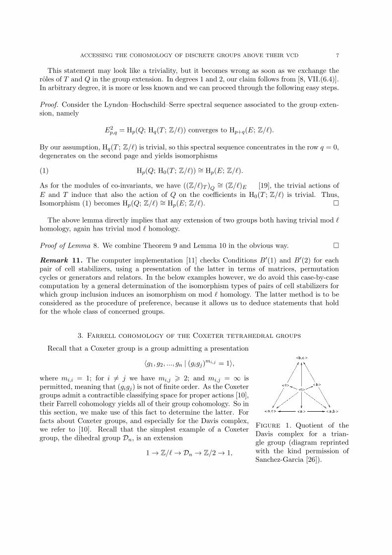
Name and Coxeter graph5−torsion

subcomplex quotientreduced 5−torsion

subcomplex quotientHq(CT (m); F5)

CT (19),b b b4 b5

CT (28)b b b5 b6

Icos120 b bD5 b D5 × Z/2 •D5 Hq(D5; F5)

CT (20),b

b

b b5

CT (22),b b b b5

CT (23),

b b

bb

5

CT (26),

b b

bb

4 5

CT (27),b

b

b b5

CT (29)

b b

bb

6 5

Icos120 b bD5 b Icos120 •D5 Hq(D5; F5)

CT (21)

b b

bb

5 5

Icos120 b bD5

b Icos120

bIcos120 bD5 b Icos120

•D5 • D5 (Hq(D5; F5))2

CT (24)b b b5 b5

Icos120 b b

D5

b D5 × Z/2

bIcos120 bD5 b D5 × Z/2

•D5 • D5 (Hq(D5; F5))2

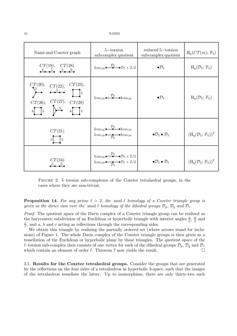
Figure 2. 5–torsion sub-complexes of the Coxeter tetrahedral groups, in thecases where they are non-trivial.

Proposition 14. For any prime ℓ > 2, the mod ℓ homology of a Coxeter triangle group isgiven as the direct sum over the mod ℓ homology of the dihedral groups Dp, Dq and Dr.

Proof. The quotient space of the Davis complex of a Coxeter triangle group can be realized asthe barycentric subdivision of an Euclidean or hyperbolic triangle with interior angles π

p, π

qand

πr, and a, b and c acting as reflections through the corresponding sides.We obtain this triangle by realizing the partially ordered set (where arrows stand for inclu-

sions) of Figure 1. The whole Davis complex of the Coxeter triangle groups is then given as atessellation of the Euclidean or hyperbolic plane by these triangles. The quotient space of theℓ–torsion sub-complex then consists of one vertex for each of the dihedral groups Dp, Dq and Dr

which contain an element of order ℓ. Theorem 7 now yields the result. �

3.1. Results for the Coxeter tetrahedral groups. Consider the groups that are generatedby the reflections on the four sides of a tetrahedron in hyperbolic 3-space, such that the imagesof the tetrahedron tessellate the latter. Up to isomorphism, there are only thirty-two such

ACCESSING THE COHOMOLOGY OF DISCRETE GROUPS ABOVE THEIR VCD 11

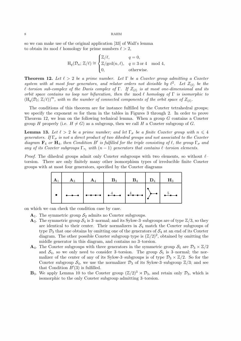
NameCoxetergraph

3−torsionsubcomplex quotient

reduced 3−torsionsubcomplex quotient

Hq(CT (m); F3)

CT (1) b b b4 b4(Z/2)3 ⋊D3b bD3 bD3 × Z/2 •D3 Hq(D3; F3)

CT (2)

b

b

b b4

4(Z/2)3 ⋊D3b bD3 b(Z/2)

3 ⋊D3 •D3 Hq(D3; F3)

CT (3)b b

bb

4

4

S4

b b

D3

b (Z/2)3 ⋊D3

bD3

b (Z/2)3 ⋊D3

•D3 Hq(D3; F3)

CT (7) b b b4 b6bD3

b (Z/2)3 ⋊D3

bD6b D6 × Z/2

•D6 • D3 (Hq(D3; F3))2

CT (8)

b

b

b b

D3b b

S4

bD3

bS4

b D3

bD3b D3 × Z/2

•D3 • D3 (Hq(D3; F3))2

CT (9)

b

b

b b4

bD3b (Z/2)3 ⋊D3

bD3b (Z/2)3 ⋊D3

bD3b D3 × Z/2

•D3 • D3 • D3 (Hq(D3; F3))3

CT (10) b b b b6

S4

b bD3

b D3 × Z/2

bD3bD6

b D6 × Z/2

•D6 • D3 (Hq(D3; F3))2

CT (11)

b

b

b b6

D3b b

D3 × Z/2b D3

b D6 •D6 • D3 (Hq(D3; F3))2

CT (12)

b

b

b b

six copies of • D3 six copies of • D3 (Hq(D3; F3))6

CT (13)

b

b

b b6 b D6b D3

b D3

bD3b D3 × Z/2 •D6 • D3 • D3 • D3 (Hq(D3; F3))

4

CT (14) b b b6 b6bD6

b D6 × Z/2

bD6b D6 × Z/2

b D3 •D6 • D6 • D3 (Hq(D3; F3))3

CT (15) b b b b6bD3

b D3 × Z/2

bD3b D3 × Z/2

b D6 •D6 • D3 • D3 (Hq(D3; F3))3

CT (16)

b

b

b bD3

b bS4

b D3

bD3b

S4 b D3b D3 •D3 • D3 • D3 (Hq(D3; F3))

3

CT (17)b b

bb

6 6 •D6 • D6 • D3 • D3 •D6 • D6 • D3 • D3 (Hq(D3; F3))4

CT (18)b b

bb

4 4 (Z/2)3 ⋊D3b bD3 b(Z/2)3 ⋊D3

(Z/2)3 ⋊D3b bD3 b(Z/2)3 ⋊D3

•D3 • D3 (Hq(D3; F3))2

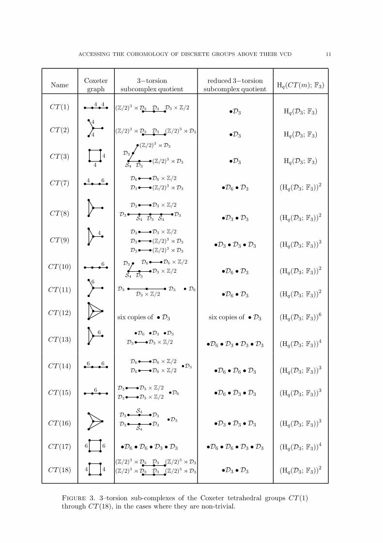
Figure 3. 3–torsion sub-complexes of the Coxeter tetrahedral groups CT (1)through CT (18), in the cases where they are non-trivial.

12 RAHM

NameCoxetergraph

3−torsionsubcomplex quotient

reduced 3−torsionsubcomplex quotient

Hq(CT (m); F3)

CT (19) b b b4 b5(Z/2)3 ⋊D3b bD3 bIcos120 •D3 Hq(D3; F3)

CT (20)

b

b

b b5

S4

b b

D3

b Icos120

bD3

b Icos120

•D3 Hq(D3; F3)

CT (21)b b

bb

5 5 Icos120 b b

D3

b Icos120

bIcos120 bD3 b Icos120

•D3 • D3 (Hq(D3; F3))2

CT (22) b b b b5Icos120 b b

D3

b D3 × Z/2

bIcos120 bD3 b D3 × Z/2

•D3 • D3 (Hq(D3; F3))2

CT (23)b b

bb

5S4

b bD3

b Icos120

bD3

bS4b

D3

b Icos120

•D3 Hq(D3; F3)

CT (24) b b b5 b5Icos120 b b

D3

b Icos120 •D3 Hq(D3; F3)

CT (25)b b

bb

4S4

b bD3

b (Z/2)3 ⋊D3

bD3

bS4b

D3

b (Z/2)3 ⋊D3

•D3 Hq(D3; F3)

CT (26)b b

bb

4 5 Icos120 b b

D3

b (Z/2)3 ⋊D3

bIcos120 bD3 b (Z/2)3 ⋊D3

•D3 • D3 (Hq(D3; F3))2

CT (27)

b

b

b b5

bD3b Icos120

bD3b Icos120

bD3b D3 × Z/2

•D3 • D3 • D3 (Hq(D3; F3))3

CT (28) b b b5 b6bD3

b Icos120

bD6b D6 × Z/2 •D6 • D3 (Hq(D3; F3))

2

CT (29)b b

bb

6 5bD3

b Icos120

bD3b Icos120 b D6 •D6 • D3 • D3 (Hq(D3; F3))

3

CT (30)b b

bb

6 4bD3

b (Z/2)3 ⋊D3

bD3b (Z/2)3 ⋊D3 b D6 •D6 • D3 • D3 (Hq(D3; F3))

3

CT (31)b b

bb

4 4

4

(Z/2)3 ⋊D3b bD3 b(Z/2)3 ⋊D3 •D3 Hq(D3; F3)

CT (32)b b

bb

6 D3b b

S4

bD3

bS4

b D3

b D6

•D6 • D3 (Hq(D3; F3))2

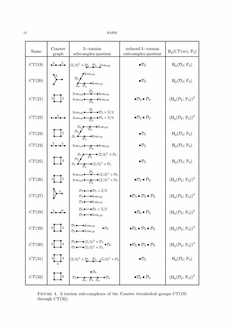
Figure 4. 3–torsion sub-complexes of the Coxeter tetrahedral groups CT (19)through CT (32).

ACCESSING THE COHOMOLOGY OF DISCRETE GROUPS ABOVE THEIR VCD 13

groups [12]; and we call them the Coxeter tetrahedral groups CT (n), with n running from 1through 32.

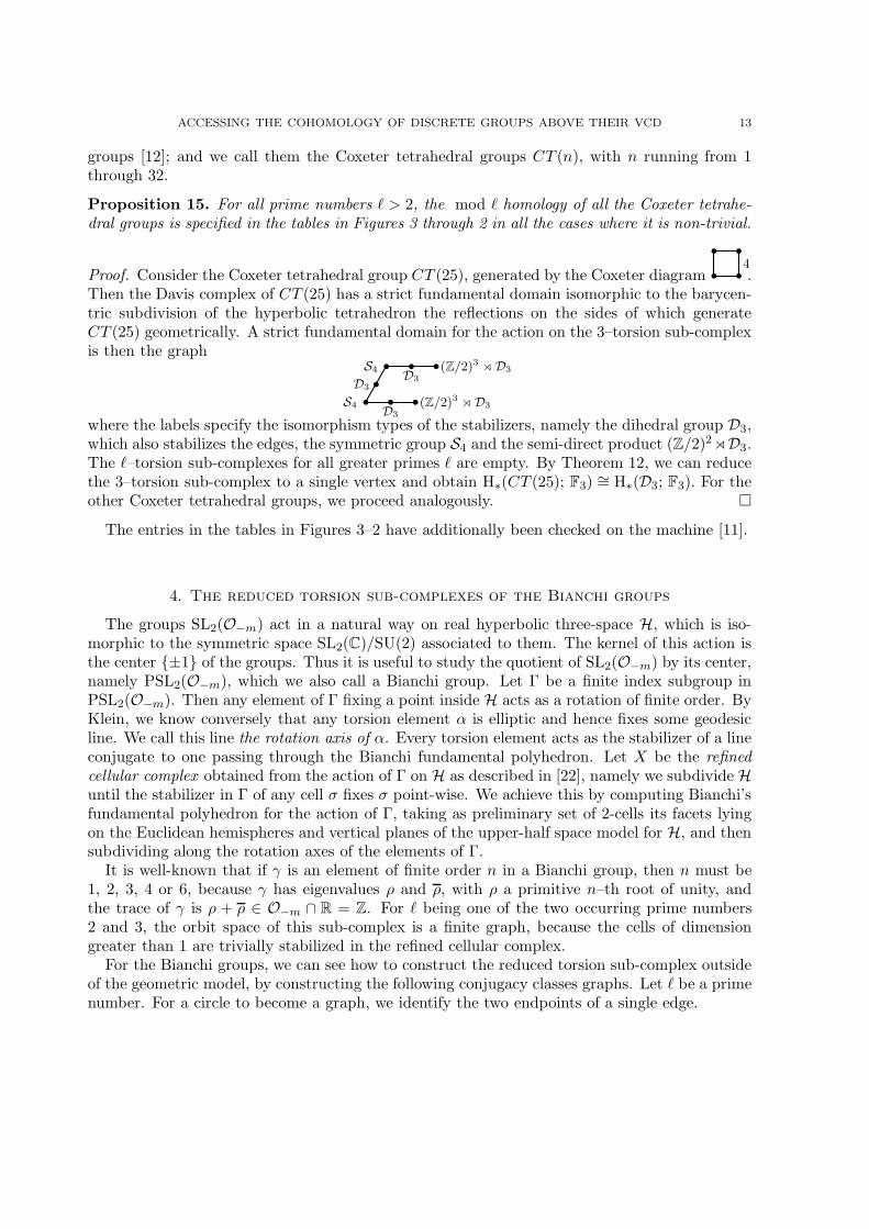
Proposition 15. For all prime numbers ℓ > 2, the mod ℓ homology of all the Coxeter tetrahe-dral groups is specified in the tables in Figures 3 through 2 in all the cases where it is non-trivial.

Proof. Consider the Coxeter tetrahedral group CT (25), generated by the Coxeter diagram b b

bb

4.

Then the Davis complex of CT (25) has a strict fundamental domain isomorphic to the barycen-tric subdivision of the hyperbolic tetrahedron the reflections on the sides of which generateCT (25) geometrically. A strict fundamental domain for the action on the 3–torsion sub-complexis then the graph

S4b b

D3

b (Z/2)3 ⋊D3

bD3

bS4b

D3

b (Z/2)3 ⋊D3

where the labels specify the isomorphism types of the stabilizers, namely the dihedral group D3,which also stabilizes the edges, the symmetric group S4 and the semi-direct product (Z/2)2⋊D3.The ℓ–torsion sub-complexes for all greater primes ℓ are empty. By Theorem 12, we can reducethe 3–torsion sub-complex to a single vertex and obtain H∗(CT (25); F3) ∼= H∗(D3; F3). For theother Coxeter tetrahedral groups, we proceed analogously. �

The entries in the tables in Figures 3–2 have additionally been checked on the machine [11].

4. The reduced torsion sub-complexes of the Bianchi groups

The groups SL2(O−m) act in a natural way on real hyperbolic three-space H, which is iso-morphic to the symmetric space SL2(C)/SU(2) associated to them. The kernel of this action isthe center {±1} of the groups. Thus it is useful to study the quotient of SL2(O−m) by its center,namely PSL2(O−m), which we also call a Bianchi group. Let Γ be a finite index subgroup inPSL2(O−m). Then any element of Γ fixing a point inside H acts as a rotation of finite order. ByKlein, we know conversely that any torsion element α is elliptic and hence fixes some geodesicline. We call this line the rotation axis of α. Every torsion element acts as the stabilizer of a lineconjugate to one passing through the Bianchi fundamental polyhedron. Let X be the refinedcellular complex obtained from the action of Γ on H as described in [22], namely we subdivide Huntil the stabilizer in Γ of any cell σ fixes σ point-wise. We achieve this by computing Bianchi’sfundamental polyhedron for the action of Γ, taking as preliminary set of 2-cells its facets lyingon the Euclidean hemispheres and vertical planes of the upper-half space model for H, and thensubdividing along the rotation axes of the elements of Γ.

It is well-known that if γ is an element of finite order n in a Bianchi group, then n must be1, 2, 3, 4 or 6, because γ has eigenvalues ρ and ρ, with ρ a primitive n–th root of unity, andthe trace of γ is ρ + ρ ∈ O−m ∩ R = Z. For ℓ being one of the two occurring prime numbers2 and 3, the orbit space of this sub-complex is a finite graph, because the cells of dimensiongreater than 1 are trivially stabilized in the refined cellular complex.

For the Bianchi groups, we can see how to construct the reduced torsion sub-complex outsideof the geometric model, by constructing the following conjugacy classes graphs. Let ℓ be a primenumber. For a circle to become a graph, we identify the two endpoints of a single edge.

14 RAHM

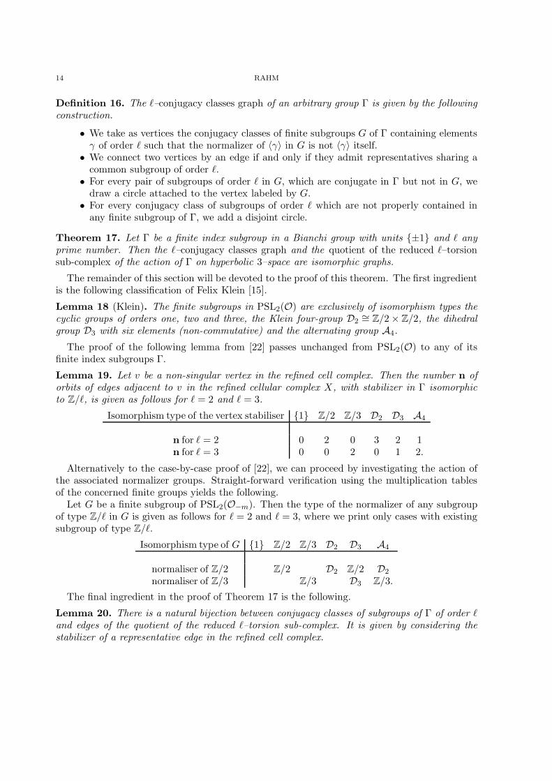
Definition 16. The ℓ–conjugacy classes graph of an arbitrary group Γ is given by the followingconstruction.

• We take as vertices the conjugacy classes of finite subgroups G of Γ containing elementsγ of order ℓ such that the normalizer of 〈γ〉 in G is not 〈γ〉 itself.

• We connect two vertices by an edge if and only if they admit representatives sharing acommon subgroup of order ℓ.

• For every pair of subgroups of order ℓ in G, which are conjugate in Γ but not in G, wedraw a circle attached to the vertex labeled by G.

• For every conjugacy class of subgroups of order ℓ which are not properly contained inany finite subgroup of Γ, we add a disjoint circle.

Theorem 17. Let Γ be a finite index subgroup in a Bianchi group with units {±1} and ℓ anyprime number. Then the ℓ–conjugacy classes graph and the quotient of the reduced ℓ–torsionsub-complex of the action of Γ on hyperbolic 3–space are isomorphic graphs.

The remainder of this section will be devoted to the proof of this theorem. The first ingredientis the following classification of Felix Klein [15].

Lemma 18 (Klein). The finite subgroups in PSL2(O) are exclusively of isomorphism types thecyclic groups of orders one, two and three, the Klein four-group D2

∼= Z/2× Z/2, the dihedralgroup D3 with six elements (non-commutative) and the alternating group A4.

The proof of the following lemma from [22] passes unchanged from PSL2(O) to any of itsfinite index subgroups Γ.

Lemma 19. Let v be a non-singular vertex in the refined cell complex. Then the number n oforbits of edges adjacent to v in the refined cellular complex X, with stabilizer in Γ isomorphicto Z/ℓ, is given as follows for ℓ = 2 and ℓ = 3.

Isomorphism type of the vertex stabiliser {1} Z/2 Z/3 D2 D3 A4

n for ℓ = 2 0 2 0 3 2 1n for ℓ = 3 0 0 2 0 1 2.

Alternatively to the case-by-case proof of [22], we can proceed by investigating the action ofthe associated normalizer groups. Straight-forward verification using the multiplication tablesof the concerned finite groups yields the following.

Let G be a finite subgroup of PSL2(O−m). Then the type of the normalizer of any subgroupof type Z/ℓ in G is given as follows for ℓ = 2 and ℓ = 3, where we print only cases with existingsubgroup of type Z/ℓ.

Isomorphism type of G {1} Z/2 Z/3 D2 D3 A4

normaliser of Z/2 Z/2 D2 Z/2 D2

normaliser of Z/3 Z/3 D3 Z/3.

The final ingredient in the proof of Theorem 17 is the following.

Lemma 20. There is a natural bijection between conjugacy classes of subgroups of Γ of order ℓand edges of the quotient of the reduced ℓ–torsion sub-complex. It is given by considering thestabilizer of a representative edge in the refined cell complex.

ACCESSING THE COHOMOLOGY OF DISCRETE GROUPS ABOVE THEIR VCD 15

In order to prove the latter lemma, we need another lemma, and we establish it now.

Remark 21. Any edge of the reduced torsion sub-complex is obtained by merging a chain ofedges on the intersection of one geodesic line with some strict fundamental domain for Γ in H.

We call this chain the chain of edges associated to α. It is well defined up to translation alongthe rotation axis of α.

Lemma 22. Let α be any non-trivial torsion element in a finite index subgroup Γ in a Bianchigroup. Then the Γ–image of the chain of edges associated to α contains the rotation axis of α.

Proof. Because of the existence of a fundamental polyhedron for the action of Γ on H, therotation axis of α is cellularly subdivided into compact edges such that the union over theΓ–orbits of finitely many of them contains all of them.

The case b . Assume that 〈α〉 ∼= Z/ℓ is not contained in any subgroup of Γ of type Dℓ.Because the inclusion Z/2 → D3, respectively Z/3 → A4, induces an isomorphism on mod 2,respectively mod 3, homology, we can merge those edges orbit-wise until the neighbouring edgesare on the same orbit. So the reduced edge admits a Γ–image containing the rotation axis of α.

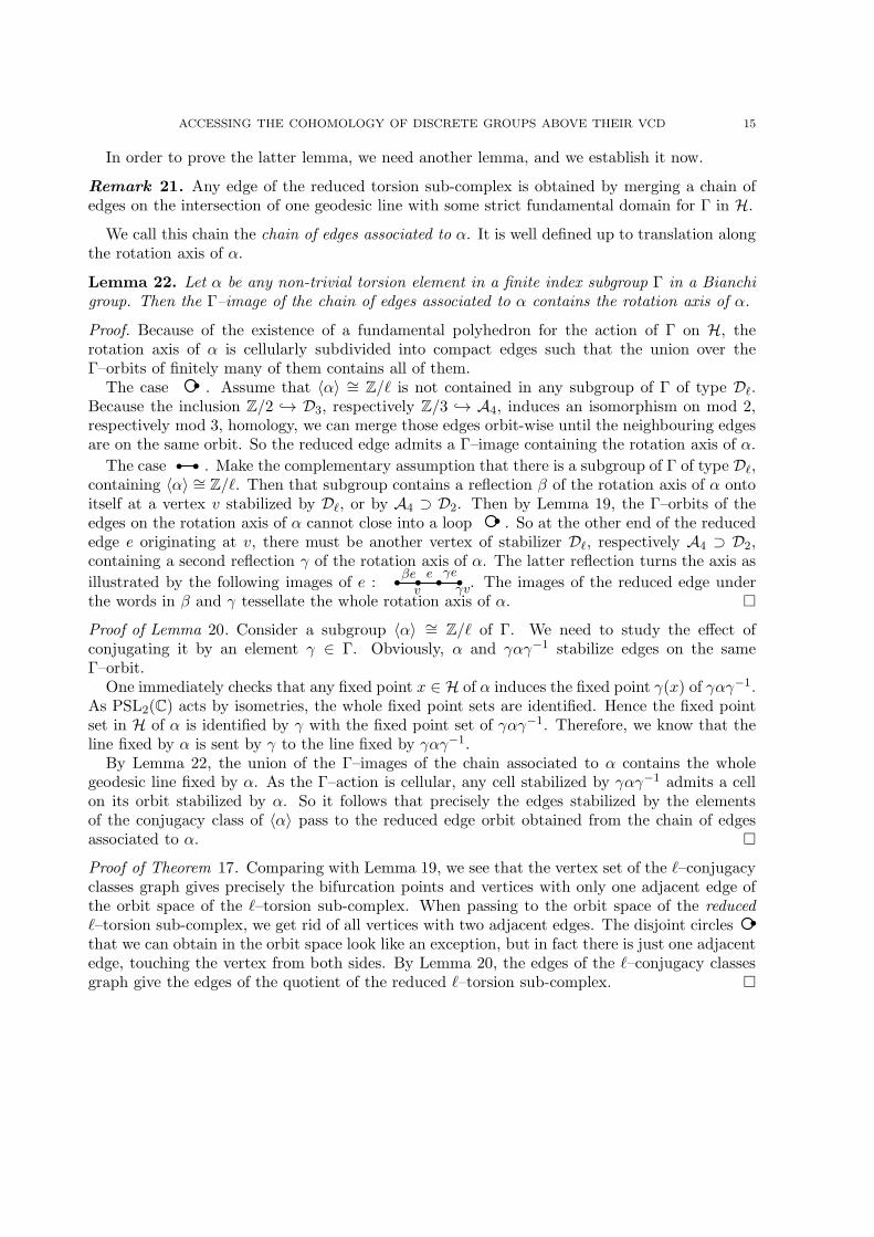
The case b b . Make the complementary assumption that there is a subgroup of Γ of type Dℓ,containing 〈α〉 ∼= Z/ℓ. Then that subgroup contains a reflection β of the rotation axis of α ontoitself at a vertex v stabilized by Dℓ, or by A4 ⊃ D2. Then by Lemma 19, the Γ–orbits of theedges on the rotation axis of α cannot close into a loop b . So at the other end of the reducededge e originating at v, there must be another vertex of stabilizer Dℓ, respectively A4 ⊃ D2,containing a second reflection γ of the rotation axis of α. The latter reflection turns the axis as

illustrated by the following images of e : b βe bv

ebγe

bγv. The images of the reduced edge under

the words in β and γ tessellate the whole rotation axis of α. �

Proof of Lemma 20. Consider a subgroup 〈α〉 ∼= Z/ℓ of Γ. We need to study the effect ofconjugating it by an element γ ∈ Γ. Obviously, α and γαγ−1 stabilize edges on the sameΓ–orbit.

One immediately checks that any fixed point x ∈ H of α induces the fixed point γ(x) of γαγ−1.As PSL2(C) acts by isometries, the whole fixed point sets are identified. Hence the fixed pointset in H of α is identified by γ with the fixed point set of γαγ−1. Therefore, we know that theline fixed by α is sent by γ to the line fixed by γαγ−1.

By Lemma 22, the union of the Γ–images of the chain associated to α contains the wholegeodesic line fixed by α. As the Γ–action is cellular, any cell stabilized by γαγ−1 admits a cellon its orbit stabilized by α. So it follows that precisely the edges stabilized by the elementsof the conjugacy class of 〈α〉 pass to the reduced edge orbit obtained from the chain of edgesassociated to α. �

Proof of Theorem 17. Comparing with Lemma 19, we see that the vertex set of the ℓ–conjugacyclasses graph gives precisely the bifurcation points and vertices with only one adjacent edge ofthe orbit space of the ℓ–torsion sub-complex. When passing to the orbit space of the reducedℓ–torsion sub-complex, we get rid of all vertices with two adjacent edges. The disjoint circles b

that we can obtain in the orbit space look like an exception, but in fact there is just one adjacentedge, touching the vertex from both sides. By Lemma 20, the edges of the ℓ–conjugacy classesgraph give the edges of the quotient of the reduced ℓ–torsion sub-complex. �

16 RAHM

5. The Farrell cohomology of the Bianchi groups

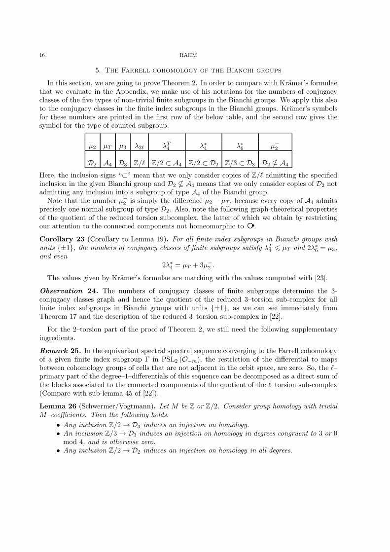
In this section, we are going to prove Theorem 2. In order to compare with Kramer’s formulaethat we evaluate in the Appendix, we make use of his notations for the numbers of conjugacyclasses of the five types of non-trivial finite subgroups in the Bianchi groups. We apply this alsoto the conjugacy classes in the finite index subgroups in the Bianchi groups. Kramer’s symbolsfor these numbers are printed in the first row of the below table, and the second row gives thesymbol for the type of counted subgroup.

µ2 µT µ3 λ2ℓ λT4 λ∗

4 λ∗6 µ−

2

D2 A4 D3 Z/ℓ Z/2 ⊂ A4 Z/2 ⊂ D2 Z/3 ⊂ D3 D2 * A4

Here, the inclusion signs “⊂” mean that we only consider copies of Z/ℓ admitting the specifiedinclusion in the given Bianchi group and D2 * A4 means that we only consider copies of D2 notadmitting any inclusion into a subgroup of type A4 of the Bianchi group.

Note that the number µ−2 is simply the difference µ2 − µT , because every copy of A4 admits

precisely one normal subgroup of type D2. Also, note the following graph-theoretical propertiesof the quotient of the reduced torsion subcomplex, the latter of which we obtain by restrictingour attention to the connected components not homeomorphic to b .

Corollary 23 (Corollary to Lemma 19). For all finite index subgroups in Bianchi groups withunits {±1}, the numbers of conjugacy classes of finite subgroups satisfy λT

4 6 µT and 2λ∗6 = µ3,

and even2λ∗

4 = µT + 3µ−2 .

The values given by Kramer’s formulae are matching with the values computed with [23].

Observation 24. The numbers of conjugacy classes of finite subgroups determine the 3-conjugacy classes graph and hence the quotient of the reduced 3–torsion sub-complex for allfinite index subgroups in Bianchi groups with units {±1}, as we can see immediately fromTheorem 17 and the description of the reduced 3–torsion sub-complex in [22].

For the 2–torsion part of the proof of Theorem 2, we still need the following supplementaryingredients.

Remark 25. In the equivariant spectral spectral sequence converging to the Farrell cohomologyof a given finite index subgroup Γ in PSL2 (O−m), the restriction of the differential to mapsbetween cohomology groups of cells that are not adjacent in the orbit space, are zero. So, the ℓ–primary part of the degree–1–differentials of this sequence can be decomposed as a direct sum ofthe blocks associated to the connected components of the quotient of the ℓ–torsion sub-complex(Compare with sub-lemma 45 of [22]).

Lemma 26 (Schwermer/Vogtmann). Let M be Z or Z/2. Consider group homology with trivialM–coefficients. Then the following holds.

• Any inclusion Z/2 → D3 induces an injection on homology.• An inclusion Z/3 → D3 induces an injection on homology in degrees congruent to 3 or 0mod 4, and is otherwise zero.

• Any inclusion Z/2 → D2 induces an injection on homology in all degrees.

ACCESSING THE COHOMOLOGY OF DISCRETE GROUPS ABOVE THEIR VCD 17

• An inclusion Z/3 → A4 induces injections on homology in all degrees.• An inclusion Z/2 → A4 induces injections on homology in degrees greater than 1, and iszero on H1.

For the proof in Z–coefficients, see [27], for Z/2–coefficients see [22].

Lemma 27 ([22], lemma 32). Let q > 3 be an odd integer number. Let v be a vertex representa-tive of stabilizer type D2 in the refined cellular complex for the Bianchi groups. Then the threeimages in (Hq(D2;Z))(2) induced by the inclusions of the stabilizers of the edges adjacent to v,

are linearly independent.

Finally, we establish the following last ingredient for the proof of Theorem 2, which might beof interest in its own right. Let Γ be a finite index subgroup in a Bianchi group, and considerits action on the refined cellular complex.

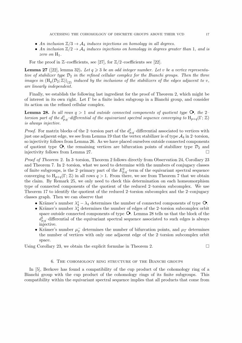
Lemma 28. In all rows q > 1 and outside connected components of quotient type b , the 2–torsion part of the d1p,q–differential of the equivariant spectral sequence converging to Hp+q(Γ; Z)is always injective.

Proof. For matrix blocks of the 2–torsion part of the d1p,q–differential associated to vertices withjust one adjacent edge, we see from Lemma 19 that the vertex stabilizer is of typeA4 in 2–torsion,so injectivity follows from Lemma 26. As we have placed ourselves outside connected componentsof quotient type b , the remaining vertices are bifurcation points of stabilizer type D2 andinjectivity follows from Lemma 27. �

Proof of Theorem 2. In 3–torsion, Theorem 2 follows directly from Observation 24, Corollary 23and Theorem 7. In 2–torsion, what we need to determine with the numbers of conjugacy classesof finite subgroups, is the 2–primary part of the E2

p,q–term of the equivariant spectral sequenceconverging to Hp+q(Γ; Z) in all rows q > 1. From there, we see from Theorem 7 that we obtainthe claim. By Remark 25, we only need to check this determination on each homeomorphismtype of connected components of the quotient of the reduced 2–torsion subcomplex. We useTheorem 17 to identify the quotient of the reduced 2–torsion subcomplex and the 2–conjugacyclasses graph. Then we can observe that

• Kramer’s number λ∗4 − λ4 determines the number of connected components of type b .

• Kramer’s number λ∗4 determines the number of edges of the 2–torsion subcomplex orbit

space outside connected components of type b . Lemma 28 tells us that the block of thed1p,q–differential of the equivariant spectral sequence associated to such edges is alwaysinjective.

• Kramer’s number µ−2 determines the number of bifurcation points, and µT determines

the number of vertices with only one adjacent edge of the 2–torsion subcomplex orbitspace.

Using Corollary 23, we obtain the explicit formulae in Theorem 2. �

6. The cohomology ring structure of the Bianchi groups

In [5], Berkove has found a compatibility of the cup product of the cohomology ring of aBianchi group with the cup product of the cohomology rings of its finite subgroups. Thiscompatibility within the equivariant spectral sequence implies that all products that come from

18 RAHM

T Subring associated to connected components of type T in the 2–conjugacy classes graph

b F2[n1](m1)

b b F2[m3, u2, v3, w3]/〈m3v3 = 0, u32 + w23 + v23 +m2

3 + w3(v3 +m3) = 0〉

b b F2[n1,m2, n3,m3]/〈n1n3 = 0, m32 +m2

3 + n23 +m3n3 + n1m2m3 = 0〉

b b F2[n1,m1,m3]/〈m3(m3 + n21m1 + n1m

21) = 0〉

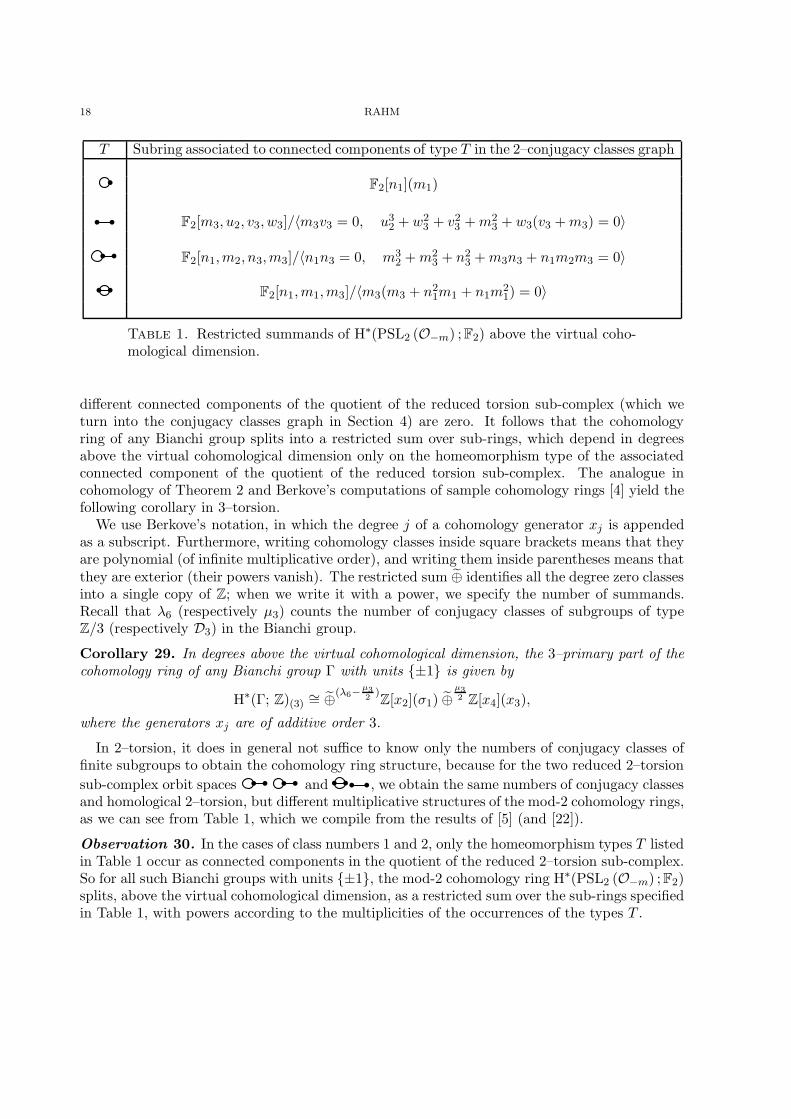
Table 1. Restricted summands of H∗(PSL2 (O−m) ;F2) above the virtual coho-mological dimension.

different connected components of the quotient of the reduced torsion sub-complex (which weturn into the conjugacy classes graph in Section 4) are zero. It follows that the cohomologyring of any Bianchi group splits into a restricted sum over sub-rings, which depend in degreesabove the virtual cohomological dimension only on the homeomorphism type of the associatedconnected component of the quotient of the reduced torsion sub-complex. The analogue incohomology of Theorem 2 and Berkove’s computations of sample cohomology rings [4] yield thefollowing corollary in 3–torsion.

We use Berkove’s notation, in which the degree j of a cohomology generator xj is appendedas a subscript. Furthermore, writing cohomology classes inside square brackets means that theyare polynomial (of infinite multiplicative order), and writing them inside parentheses means thatthey are exterior (their powers vanish). The restricted sum ⊕ identifies all the degree zero classesinto a single copy of Z; when we write it with a power, we specify the number of summands.Recall that λ6 (respectively µ3) counts the number of conjugacy classes of subgroups of typeZ/3 (respectively D3) in the Bianchi group.

Corollary 29. In degrees above the virtual cohomological dimension, the 3–primary part of thecohomology ring of any Bianchi group Γ with units {±1} is given by

H∗(Γ; Z)(3) ∼= ⊕(λ6−µ32)Z[x2](σ1) ⊕

µ32 Z[x4](x3),

where the generators xj are of additive order 3.

In 2–torsion, it does in general not suffice to know only the numbers of conjugacy classes offinite subgroups to obtain the cohomology ring structure, because for the two reduced 2–torsion

sub-complex orbit spaces b b b b and b b b b , we obtain the same numbers of conjugacy classesand homological 2–torsion, but different multiplicative structures of the mod-2 cohomology rings,as we can see from Table 1, which we compile from the results of [5] (and [22]).

Observation 30. In the cases of class numbers 1 and 2, only the homeomorphism types T listedin Table 1 occur as connected components in the quotient of the reduced 2–torsion sub-complex.So for all such Bianchi groups with units {±1}, the mod-2 cohomology ring H∗(PSL2 (O−m) ;F2)splits, above the virtual cohomological dimension, as a restricted sum over the sub-rings specifiedin Table 1, with powers according to the multiplicities of the occurrences of the types T .

ACCESSING THE COHOMOLOGY OF DISCRETE GROUPS ABOVE THEIR VCD 19

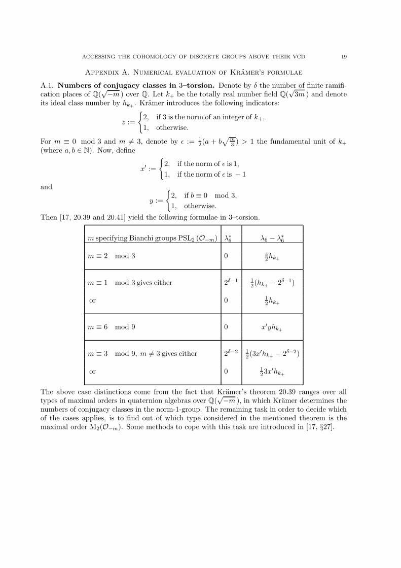
Appendix A. Numerical evaluation of Kramer’s formulae

A.1. Numbers of conjugacy classes in 3–torsion. Denote by δ the number of finite ramifi-cation places of Q(

√−m ) over Q. Let k+ be the totally real number field Q(√3m ) and denote

its ideal class number by hk+ . Kramer introduces the following indicators:

z :=

{2, if 3 is the norm of an integer of k+,

1, otherwise.

For m ≡ 0 mod 3 and m 6= 3, denote by ǫ := 12(a + b

√m3 ) > 1 the fundamental unit of k+

(where a, b ∈ N). Now, define

x′ :=

{2, if the norm of ǫ is 1,

1, if the norm of ǫ is − 1

and

y :=

{2, if b ≡ 0 mod 3,

1, otherwise.

Then [17, 20.39 and 20.41] yield the following formulae in 3–torsion.

m specifying Bianchi groups PSL2 (O−m) λ∗6 λ6 − λ∗

6

m ≡ 2 mod 3 0 z2hk+

m ≡ 1 mod 3 gives either 2δ−1 12(hk+ − 2δ−1)

or 0 12hk+

m ≡ 6 mod 9 0 x′yhk+

m ≡ 3 mod 9, m 6= 3 gives either 2δ−2 12(3x

′hk+ − 2δ−2)

or 0 123x

′hk+

The above case distinctions come from the fact that Kramer’s theorem 20.39 ranges over alltypes of maximal orders in quaternion algebras over Q(

√−m ), in which Kramer determines the

numbers of conjugacy classes in the norm-1-group. The remaining task in order to decide whichof the cases applies, is to find out of which type considered in the mentioned theorem is themaximal order M2(O−m). Some methods to cope with this task are introduced in [17, §27].

20 RAHM

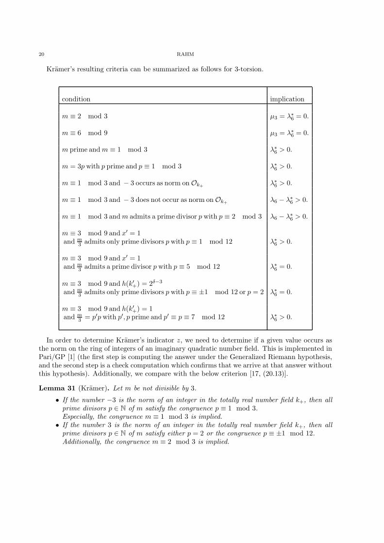
Kramer’s resulting criteria can be summarized as follows for 3-torsion.

condition implication

m ≡ 2 mod 3 µ3 = λ∗6 = 0.

m ≡ 6 mod 9 µ3 = λ∗6 = 0.

m prime andm ≡ 1 mod 3 λ∗6 > 0.

m = 3p with p prime and p ≡ 1 mod 3 λ∗6 > 0.

m ≡ 1 mod 3 and − 3 occurs as norm onOk+ λ∗6 > 0.

m ≡ 1 mod 3 and − 3 does not occur as norm onOk+ λ6 − λ∗6 > 0.

m ≡ 1 mod 3 andm admits a prime divisor p with p ≡ 2 mod 3 λ6 − λ∗6 > 0.

m ≡ 3 mod 9 and x′ = 1and m

3 admits only prime divisors p with p ≡ 1 mod 12 λ∗6 > 0.

m ≡ 3 mod 9 and x′ = 1and m

3 admits a prime divisor p with p ≡ 5 mod 12 λ∗6 = 0.

m ≡ 3 mod 9 and h(k′+) = 2δ−3

and m3 admits only prime divisors p with p ≡ ±1 mod 12 or p = 2 λ∗

6 = 0.

m ≡ 3 mod 9 and h(k′+) = 1and m

3 = p′p with p′, p prime and p′ ≡ p ≡ 7 mod 12 λ∗6 > 0.

In order to determine Kramer’s indicator z, we need to determine if a given value occurs asthe norm on the ring of integers of an imaginary quadratic number field. This is implemented inPari/GP [1] (the first step is computing the answer under the Generalized Riemann hypothesis,and the second step is a check computation which confirms that we arrive at that answer withoutthis hypothesis). Additionally, we compare with the below criterion [17, (20.13)].

Lemma 31 (Kramer). Let m be not divisible by 3.

• If the number −3 is the norm of an integer in the totally real number field k+, then allprime divisors p ∈ N of m satisfy the congruence p ≡ 1 mod 3.Especially, the congruence m ≡ 1 mod 3 is implied.

• If the number 3 is the norm of an integer in the totally real number field k+, then allprime divisors p ∈ N of m satisfy either p = 2 or the congruence p ≡ ±1 mod 12.Additionally, the congruence m ≡ 2 mod 3 is implied.

ACCESSING THE COHOMOLOGY OF DISCRETE GROUPS ABOVE THEIR VCD 21

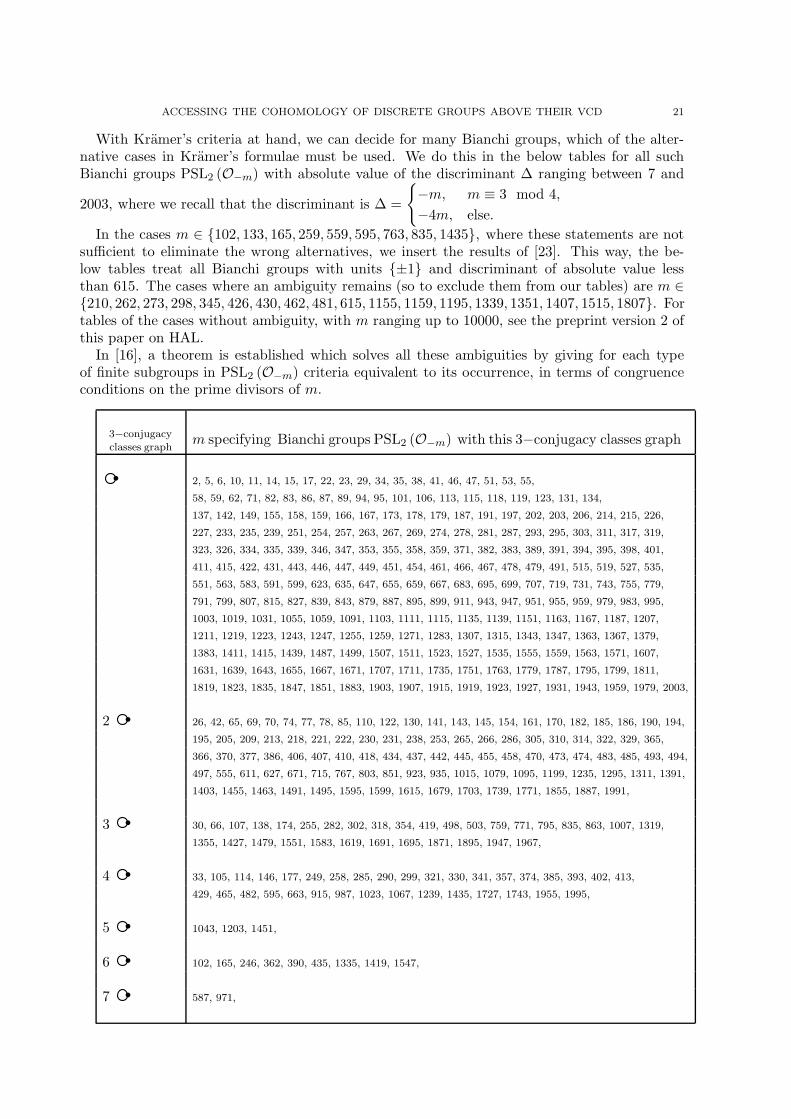
With Kramer’s criteria at hand, we can decide for many Bianchi groups, which of the alter-native cases in Kramer’s formulae must be used. We do this in the below tables for all suchBianchi groups PSL2 (O−m) with absolute value of the discriminant ∆ ranging between 7 and

2003, where we recall that the discriminant is ∆ =

{−m, m ≡ 3 mod 4,

−4m, else.

In the cases m ∈ {102, 133, 165, 259, 559, 595, 763, 835, 1435}, where these statements are notsufficient to eliminate the wrong alternatives, we insert the results of [23]. This way, the be-low tables treat all Bianchi groups with units {±1} and discriminant of absolute value lessthan 615. The cases where an ambiguity remains (so to exclude them from our tables) are m ∈{210, 262, 273, 298, 345, 426, 430, 462, 481, 615, 1155, 1159, 1195, 1339, 1351, 1407, 1515, 1807}. Fortables of the cases without ambiguity, with m ranging up to 10000, see the preprint version 2 ofthis paper on HAL.

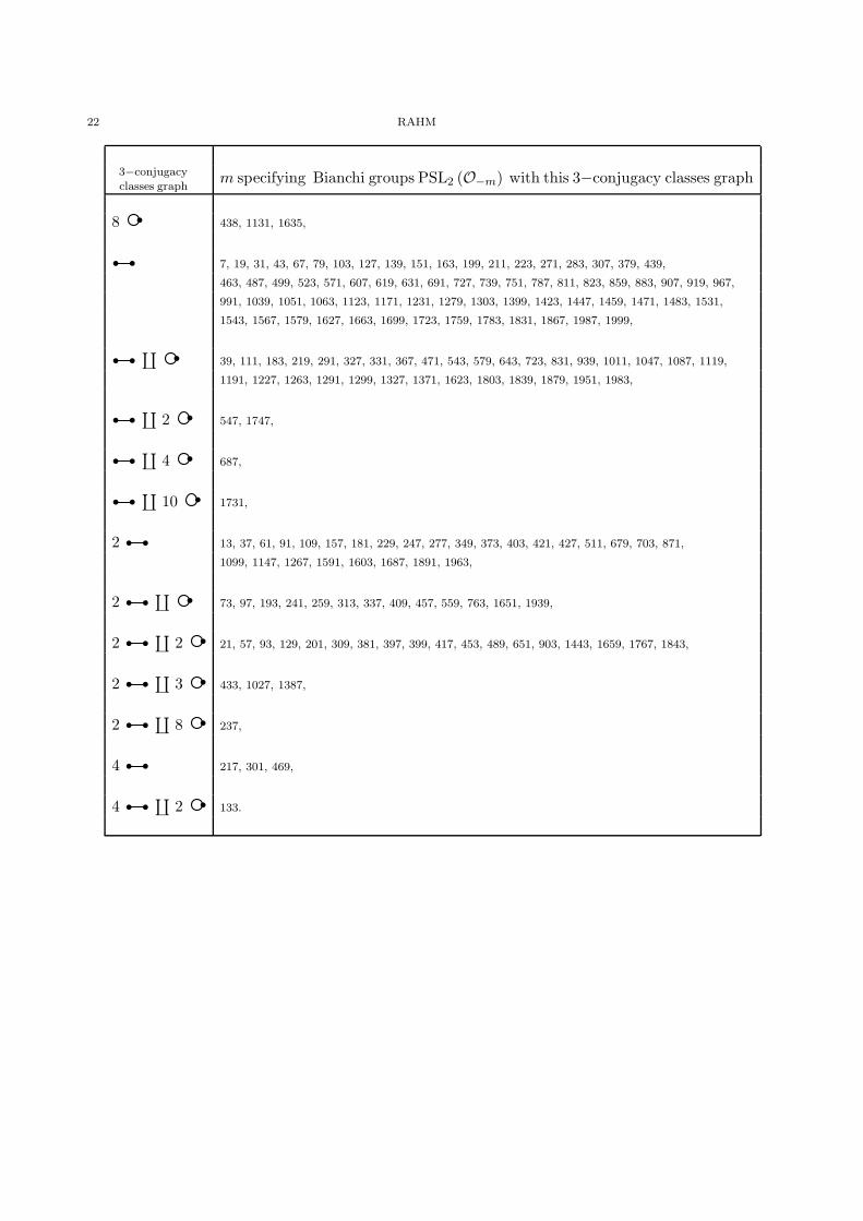
In [16], a theorem is established which solves all these ambiguities by giving for each typeof finite subgroups in PSL2 (O−m) criteria equivalent to its occurrence, in terms of congruenceconditions on the prime divisors of m.

3−conjugacyclasses graph

m specifying Bianchi groups PSL2 (O−m) with this 3−conjugacy classes graph

b2, 5, 6, 10, 11, 14, 15, 17, 22, 23, 29, 34, 35, 38, 41, 46, 47, 51, 53, 55,

58, 59, 62, 71, 82, 83, 86, 87, 89, 94, 95, 101, 106, 113, 115, 118, 119, 123, 131, 134,

137, 142, 149, 155, 158, 159, 166, 167, 173, 178, 179, 187, 191, 197, 202, 203, 206, 214, 215, 226,

227, 233, 235, 239, 251, 254, 257, 263, 267, 269, 274, 278, 281, 287, 293, 295, 303, 311, 317, 319,

323, 326, 334, 335, 339, 346, 347, 353, 355, 358, 359, 371, 382, 383, 389, 391, 394, 395, 398, 401,

411, 415, 422, 431, 443, 446, 447, 449, 451, 454, 461, 466, 467, 478, 479, 491, 515, 519, 527, 535,

551, 563, 583, 591, 599, 623, 635, 647, 655, 659, 667, 683, 695, 699, 707, 719, 731, 743, 755, 779,

791, 799, 807, 815, 827, 839, 843, 879, 887, 895, 899, 911, 943, 947, 951, 955, 959, 979, 983, 995,

1003, 1019, 1031, 1055, 1059, 1091, 1103, 1111, 1115, 1135, 1139, 1151, 1163, 1167, 1187, 1207,

1211, 1219, 1223, 1243, 1247, 1255, 1259, 1271, 1283, 1307, 1315, 1343, 1347, 1363, 1367, 1379,

1383, 1411, 1415, 1439, 1487, 1499, 1507, 1511, 1523, 1527, 1535, 1555, 1559, 1563, 1571, 1607,

1631, 1639, 1643, 1655, 1667, 1671, 1707, 1711, 1735, 1751, 1763, 1779, 1787, 1795, 1799, 1811,

1819, 1823, 1835, 1847, 1851, 1883, 1903, 1907, 1915, 1919, 1923, 1927, 1931, 1943, 1959, 1979, 2003,

2 b26, 42, 65, 69, 70, 74, 77, 78, 85, 110, 122, 130, 141, 143, 145, 154, 161, 170, 182, 185, 186, 190, 194,

195, 205, 209, 213, 218, 221, 222, 230, 231, 238, 253, 265, 266, 286, 305, 310, 314, 322, 329, 365,

366, 370, 377, 386, 406, 407, 410, 418, 434, 437, 442, 445, 455, 458, 470, 473, 474, 483, 485, 493, 494,

497, 555, 611, 627, 671, 715, 767, 803, 851, 923, 935, 1015, 1079, 1095, 1199, 1235, 1295, 1311, 1391,

1403, 1455, 1463, 1491, 1495, 1595, 1599, 1615, 1679, 1703, 1739, 1771, 1855, 1887, 1991,

3 b30, 66, 107, 138, 174, 255, 282, 302, 318, 354, 419, 498, 503, 759, 771, 795, 835, 863, 1007, 1319,

1355, 1427, 1479, 1551, 1583, 1619, 1691, 1695, 1871, 1895, 1947, 1967,

4 b33, 105, 114, 146, 177, 249, 258, 285, 290, 299, 321, 330, 341, 357, 374, 385, 393, 402, 413,

429, 465, 482, 595, 663, 915, 987, 1023, 1067, 1239, 1435, 1727, 1743, 1955, 1995,

5 b1043, 1203, 1451,

6 b102, 165, 246, 362, 390, 435, 1335, 1419, 1547,

7 b587, 971,

22 RAHM

3−conjugacyclasses graph

m specifying Bianchi groups PSL2 (O−m) with this 3−conjugacy classes graph

8 b438, 1131, 1635,

b b 7, 19, 31, 43, 67, 79, 103, 127, 139, 151, 163, 199, 211, 223, 271, 283, 307, 379, 439,

463, 487, 499, 523, 571, 607, 619, 631, 691, 727, 739, 751, 787, 811, 823, 859, 883, 907, 919, 967,

991, 1039, 1051, 1063, 1123, 1171, 1231, 1279, 1303, 1399, 1423, 1447, 1459, 1471, 1483, 1531,

1543, 1567, 1579, 1627, 1663, 1699, 1723, 1759, 1783, 1831, 1867, 1987, 1999,

b b∐

b39, 111, 183, 219, 291, 327, 331, 367, 471, 543, 579, 643, 723, 831, 939, 1011, 1047, 1087, 1119,

1191, 1227, 1263, 1291, 1299, 1327, 1371, 1623, 1803, 1839, 1879, 1951, 1983,

b b∐

2 b547, 1747,

b b∐

4 b687,

b b∐

10 b1731,

2 b b 13, 37, 61, 91, 109, 157, 181, 229, 247, 277, 349, 373, 403, 421, 427, 511, 679, 703, 871,

1099, 1147, 1267, 1591, 1603, 1687, 1891, 1963,

2 b b∐

b73, 97, 193, 241, 259, 313, 337, 409, 457, 559, 763, 1651, 1939,

2 b b∐

2 b21, 57, 93, 129, 201, 309, 381, 397, 399, 417, 453, 489, 651, 903, 1443, 1659, 1767, 1843,

2 b b∐

3 b433, 1027, 1387,

2 b b∐

8 b237,

4 b b 217, 301, 469,

4 b b∐

2 b133.

ACCESSING THE COHOMOLOGY OF DISCRETE GROUPS ABOVE THEIR VCD 23

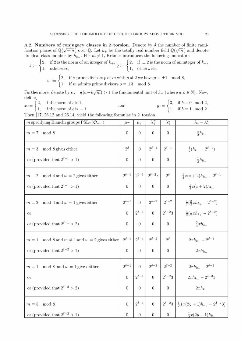
A.2. Numbers of conjugacy classes in 2–torsion. Denote by δ the number of finite rami-fication places of Q(

√−m ) over Q. Let k+ be the totally real number field Q(

√m ) and denote

its ideal class number by hk+ . For m 6= 1, Kramer introduces the following indicators:

z :=

{2, if 2 is the norm of an integer of k+,

1, otherwise,q :=

{2, if ± 2 is the norm of an integer of k+,

1, otherwise,

w :=

{2, if ∀ prime divisors p of m with p 6= 2 we have p ≡ ±1 mod 8,

1, if m admits prime divisors p ≡ ±3 mod 8.

Furthermore, denote by ǫ := 12 (a+b

√m) > 1 the fundamental unit of k+ (where a, b ∈ N). Now,

define

x :=

{2, if the norm of ǫ is 1,

1, if the norm of ǫ is − 1and y :=

{3, if b ≡ 0 mod 2,

1, if b ≡ 1 mod 2.

Then [17, 26.12 and 26.14] yield the following formulae in 2–torsion.

m specifying Bianchi groups PSL2 (O−m) µT µ−2 λT

4 λ∗4 λ4 − λ∗

4

m ≡ 7 mod 8 0 0 0 0 z2hk+

m ≡ 3 mod 8 gives either 2δ 0 2δ−1 2δ−1 12(hk+ − 2δ−1)

or (provided that 2δ−1 > 1) 0 0 0 0 12hk+

m ≡ 2 mod 4 and w = 2 gives either 2δ−1 2δ−1 2δ−2z 2δ 14x(z + 2)hk+ − 2δ−1

or (provided that 2δ−1 > 1) 0 0 0 0 14x(z + 2)hk+

m ≡ 2 mod 4 and w = 1 gives either 2δ−1 0 2δ−2 2δ−2 12(

32xhk+ − 2δ−2)

or 0 2δ−1 0 2δ−23 32(

12xhk+ − 2δ−2)

or (provided that 2δ−1 > 2) 0 0 0 0 34xhk+

m ≡ 1 mod 8 andm 6= 1 and w = 2 gives either 2δ−1 2δ−1 2δ−2 2δ 2xhk+ − 2δ−1

or (provided that 2δ−2 > 1) 0 0 0 0 2xhk+

m ≡ 1 mod 8 and w = 1 gives either 2δ−1 0 2δ−2 2δ−2 2xhk+ − 2δ−3

or 0 2δ−1 0 2δ−23 2xhk+ − 2δ−33

or (provided that 2δ−2 > 2) 0 0 0 0 2xhk+

m ≡ 5 mod 8 0 2δ−1 0 2δ−23 12

(x(2y + 1)hk+ − 2δ−23

)

or (provided that 2δ−2 > 1) 0 0 0 0 12x(2y + 1)hk+

24 RAHM

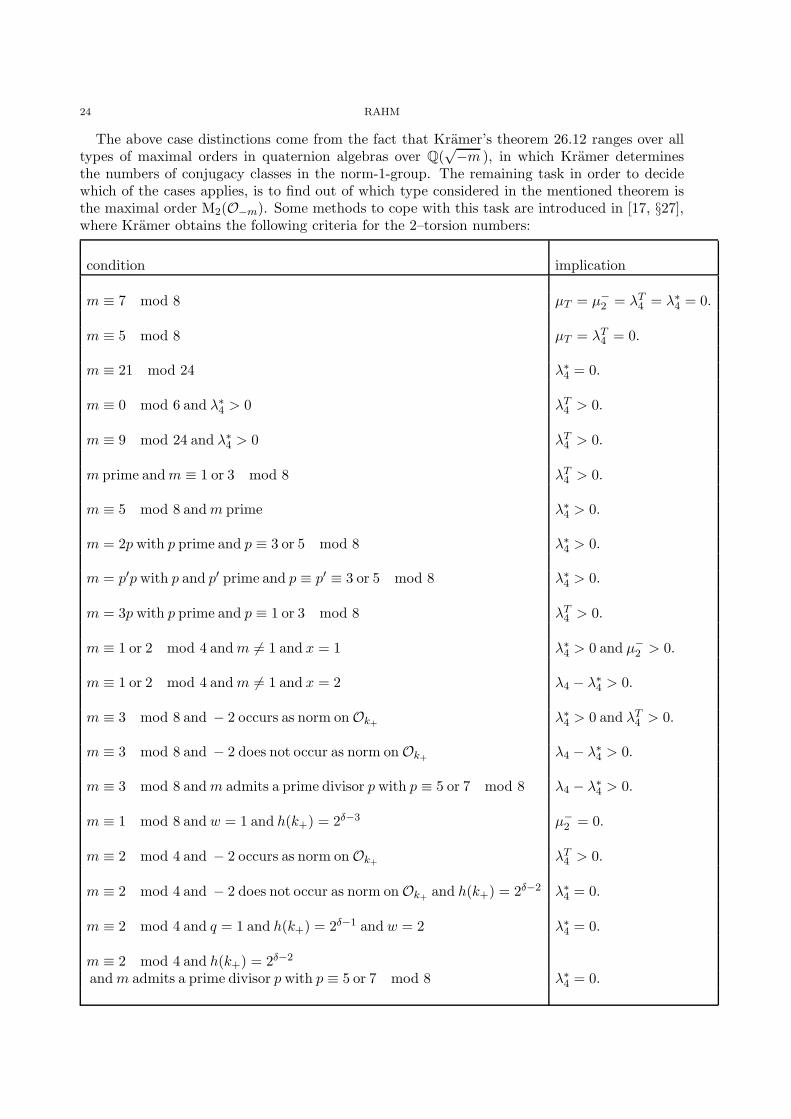
The above case distinctions come from the fact that Kramer’s theorem 26.12 ranges over alltypes of maximal orders in quaternion algebras over Q(

√−m ), in which Kramer determines

the numbers of conjugacy classes in the norm-1-group. The remaining task in order to decidewhich of the cases applies, is to find out of which type considered in the mentioned theorem isthe maximal order M2(O−m). Some methods to cope with this task are introduced in [17, §27],where Kramer obtains the following criteria for the 2–torsion numbers:

condition implication

m ≡ 7 mod 8 µT = µ−2 = λT

4 = λ∗4 = 0.

m ≡ 5 mod 8 µT = λT4 = 0.

m ≡ 21 mod 24 λ∗4 = 0.

m ≡ 0 mod 6 and λ∗4 > 0 λT

4 > 0.

m ≡ 9 mod 24 and λ∗4 > 0 λT

4 > 0.

m prime andm ≡ 1 or 3 mod 8 λT4 > 0.

m ≡ 5 mod 8 andm prime λ∗4 > 0.

m = 2p with p prime and p ≡ 3 or 5 mod 8 λ∗4 > 0.

m = p′p with p and p′ prime and p ≡ p′ ≡ 3 or 5 mod 8 λ∗4 > 0.

m = 3p with p prime and p ≡ 1 or 3 mod 8 λT4 > 0.

m ≡ 1 or 2 mod 4 andm 6= 1 and x = 1 λ∗4 > 0 and µ−

2 > 0.

m ≡ 1 or 2 mod 4 andm 6= 1 and x = 2 λ4 − λ∗4 > 0.

m ≡ 3 mod 8 and − 2 occurs as norm onOk+ λ∗4 > 0 and λT

4 > 0.

m ≡ 3 mod 8 and − 2 does not occur as norm onOk+ λ4 − λ∗4 > 0.

m ≡ 3 mod 8 andm admits a prime divisor p with p ≡ 5 or 7 mod 8 λ4 − λ∗4 > 0.

m ≡ 1 mod 8 and w = 1 and h(k+) = 2δ−3 µ−2 = 0.

m ≡ 2 mod 4 and − 2 occurs as norm onOk+ λT4 > 0.

m ≡ 2 mod 4 and − 2 does not occur as norm onOk+ and h(k+) = 2δ−2 λ∗4 = 0.

m ≡ 2 mod 4 and q = 1 and h(k+) = 2δ−1 and w = 2 λ∗4 = 0.

m ≡ 2 mod 4 and h(k+) = 2δ−2

andm admits a prime divisor p with p ≡ 5 or 7 mod 8 λ∗4 = 0.

ACCESSING THE COHOMOLOGY OF DISCRETE GROUPS ABOVE THEIR VCD 25

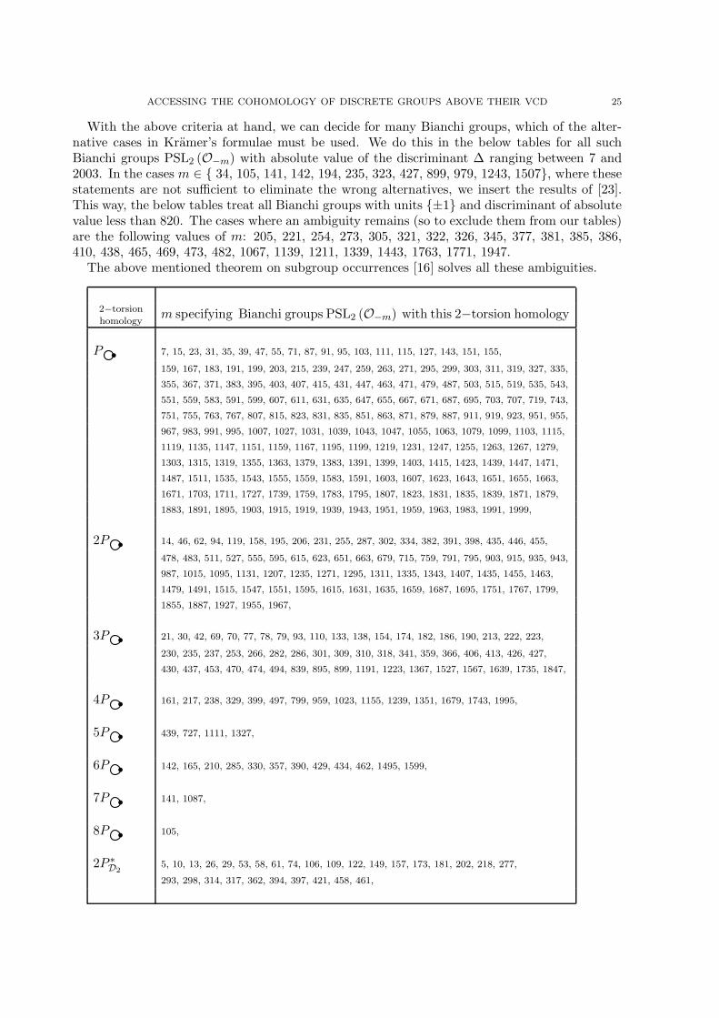
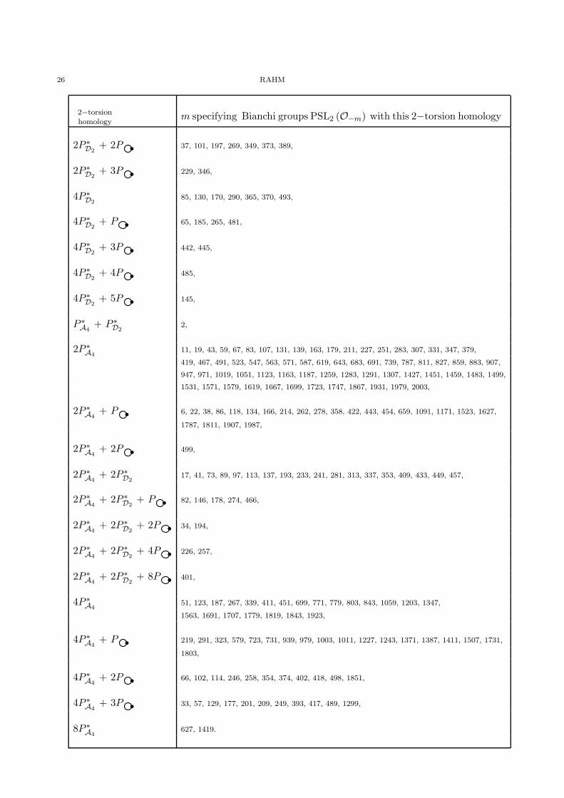
With the above criteria at hand, we can decide for many Bianchi groups, which of the alter-native cases in Kramer’s formulae must be used. We do this in the below tables for all suchBianchi groups PSL2 (O−m) with absolute value of the discriminant ∆ ranging between 7 and2003. In the cases m ∈ { 34, 105, 141, 142, 194, 235, 323, 427, 899, 979, 1243, 1507}, where thesestatements are not sufficient to eliminate the wrong alternatives, we insert the results of [23].This way, the below tables treat all Bianchi groups with units {±1} and discriminant of absolutevalue less than 820. The cases where an ambiguity remains (so to exclude them from our tables)are the following values of m: 205, 221, 254, 273, 305, 321, 322, 326, 345, 377, 381, 385, 386,410, 438, 465, 469, 473, 482, 1067, 1139, 1211, 1339, 1443, 1763, 1771, 1947.

The above mentioned theorem on subgroup occurrences [16] solves all these ambiguities.

2−torsionhomology

m specifying Bianchi groups PSL2 (O−m) with this 2−torsion homology

P b 7, 15, 23, 31, 35, 39, 47, 55, 71, 87, 91, 95, 103, 111, 115, 127, 143, 151, 155,

159, 167, 183, 191, 199, 203, 215, 239, 247, 259, 263, 271, 295, 299, 303, 311, 319, 327, 335,

355, 367, 371, 383, 395, 403, 407, 415, 431, 447, 463, 471, 479, 487, 503, 515, 519, 535, 543,

551, 559, 583, 591, 599, 607, 611, 631, 635, 647, 655, 667, 671, 687, 695, 703, 707, 719, 743,

751, 755, 763, 767, 807, 815, 823, 831, 835, 851, 863, 871, 879, 887, 911, 919, 923, 951, 955,

967, 983, 991, 995, 1007, 1027, 1031, 1039, 1043, 1047, 1055, 1063, 1079, 1099, 1103, 1115,

1119, 1135, 1147, 1151, 1159, 1167, 1195, 1199, 1219, 1231, 1247, 1255, 1263, 1267, 1279,

1303, 1315, 1319, 1355, 1363, 1379, 1383, 1391, 1399, 1403, 1415, 1423, 1439, 1447, 1471,

1487, 1511, 1535, 1543, 1555, 1559, 1583, 1591, 1603, 1607, 1623, 1643, 1651, 1655, 1663,

1671, 1703, 1711, 1727, 1739, 1759, 1783, 1795, 1807, 1823, 1831, 1835, 1839, 1871, 1879,

1883, 1891, 1895, 1903, 1915, 1919, 1939, 1943, 1951, 1959, 1963, 1983, 1991, 1999,

2P b 14, 46, 62, 94, 119, 158, 195, 206, 231, 255, 287, 302, 334, 382, 391, 398, 435, 446, 455,

478, 483, 511, 527, 555, 595, 615, 623, 651, 663, 679, 715, 759, 791, 795, 903, 915, 935, 943,

987, 1015, 1095, 1131, 1207, 1235, 1271, 1295, 1311, 1335, 1343, 1407, 1435, 1455, 1463,

1479, 1491, 1515, 1547, 1551, 1595, 1615, 1631, 1635, 1659, 1687, 1695, 1751, 1767, 1799,

1855, 1887, 1927, 1955, 1967,

3P b 21, 30, 42, 69, 70, 77, 78, 79, 93, 110, 133, 138, 154, 174, 182, 186, 190, 213, 222, 223,

230, 235, 237, 253, 266, 282, 286, 301, 309, 310, 318, 341, 359, 366, 406, 413, 426, 427,

430, 437, 453, 470, 474, 494, 839, 895, 899, 1191, 1223, 1367, 1527, 1567, 1639, 1735, 1847,

4P b 161, 217, 238, 329, 399, 497, 799, 959, 1023, 1155, 1239, 1351, 1679, 1743, 1995,

5P b 439, 727, 1111, 1327,

6P b 142, 165, 210, 285, 330, 357, 390, 429, 434, 462, 1495, 1599,

7P b 141, 1087,

8P b 105,

2P ∗D2

5, 10, 13, 26, 29, 53, 58, 61, 74, 106, 109, 122, 149, 157, 173, 181, 202, 218, 277,

293, 298, 314, 317, 362, 394, 397, 421, 458, 461,

26 RAHM

2−torsionhomology

m specifying Bianchi groups PSL2 (O−m) with this 2−torsion homology

2P ∗D2

+ 2P b 37, 101, 197, 269, 349, 373, 389,

2P ∗D2

+ 3P b 229, 346,

4P ∗D2

85, 130, 170, 290, 365, 370, 493,

4P ∗D2

+ P b 65, 185, 265, 481,

4P ∗D2

+ 3P b 442, 445,

4P ∗D2

+ 4P b 485,

4P ∗D2

+ 5P b 145,

P ∗A4

+ P ∗D2

2,

2P ∗A4

11, 19, 43, 59, 67, 83, 107, 131, 139, 163, 179, 211, 227, 251, 283, 307, 331, 347, 379,

419, 467, 491, 523, 547, 563, 571, 587, 619, 643, 683, 691, 739, 787, 811, 827, 859, 883, 907,

947, 971, 1019, 1051, 1123, 1163, 1187, 1259, 1283, 1291, 1307, 1427, 1451, 1459, 1483, 1499,

1531, 1571, 1579, 1619, 1667, 1699, 1723, 1747, 1867, 1931, 1979, 2003,

2P ∗A4

+ P b 6, 22, 38, 86, 118, 134, 166, 214, 262, 278, 358, 422, 443, 454, 659, 1091, 1171, 1523, 1627,

1787, 1811, 1907, 1987,

2P ∗A4

+ 2P b 499,

2P ∗A4

+ 2P ∗D2

17, 41, 73, 89, 97, 113, 137, 193, 233, 241, 281, 313, 337, 353, 409, 433, 449, 457,

2P ∗A4

+ 2P ∗D2

+ P b 82, 146, 178, 274, 466,

2P ∗A4

+ 2P ∗D2

+ 2P b 34, 194,

2P ∗A4

+ 2P ∗D2

+ 4P b 226, 257,

2P ∗A4

+ 2P ∗D2

+ 8P b 401,

4P ∗A4

51, 123, 187, 267, 339, 411, 451, 699, 771, 779, 803, 843, 1059, 1203, 1347,

1563, 1691, 1707, 1779, 1819, 1843, 1923,

4P ∗A4

+ P b 219, 291, 323, 579, 723, 731, 939, 979, 1003, 1011, 1227, 1243, 1371, 1387, 1411, 1507, 1731,

1803,

4P ∗A4

+ 2P b 66, 102, 114, 246, 258, 354, 374, 402, 418, 498, 1851,

4P ∗A4

+ 3P b 33, 57, 129, 177, 201, 209, 249, 393, 417, 489, 1299,

8P ∗A4

627, 1419.

ACCESSING THE COHOMOLOGY OF DISCRETE GROUPS ABOVE THEIR VCD 27

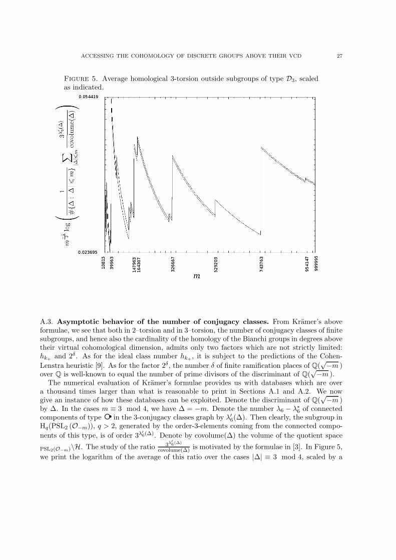
Figure 5. Average homological 3-torsion outside subgroups of type D3, scaledas indicated.

A.3. Asymptotic behavior of the number of conjugacy classes. From Kramer’s aboveformulae, we see that both in 2–torsion and in 3–torsion, the number of conjugacy classes of finitesubgroups, and hence also the cardinality of the homology of the Bianchi groups in degrees abovetheir virtual cohomological dimension, admits only two factors which are not strictly limited:hk+ and 2δ . As for the ideal class number hk+ , it is subject to the predictions of the Cohen-

Lenstra heuristic [9]. As for the factor 2δ, the number δ of finite ramification places of Q(√−m )

over Q is well-known to equal the number of prime divisors of the discriminant of Q(√−m ).

The numerical evaluation of Kramer’s formulae provides us with databases which are overa thousand times larger than what is reasonable to print in Sections A.1 and A.2. We nowgive an instance of how these databases can be exploited. Denote the discriminant of Q(

√−m )

by ∆. In the cases m ≡ 3 mod 4, we have ∆ = −m. Denote the number λ6 − λ∗6 of connected

components of type b in the 3-conjugacy classes graph by λ′6(∆). Then clearly, the subgroup in

Hq(PSL2 (O−m)), q > 2, generated by the order-3-elements coming from the connected compo-

nents of this type, is of order 3λ′

6(∆). Denote by covolume(∆) the volume of the quotient space

PSL2(O−m)\H. The study of the ratio 3λ′

6(∆)

covolume(∆) is motivated by the formulae in [3]. In Figure 5,

we print the logarithm of the average of this ratio over the cases |∆| ≡ 3 mod 4, scaled by a

28 RAHM

factor m−23 , so to say

m−23 log

1

#{∆ : |∆| 6 m}∑

|∆|6m

3λ′

6(∆)

covolume(∆)

,

where we consider m and ∆ as independent variables, m running through the square-free positiverational integers. In order to cope with the fact that in some cases, Kramer’s formulae leave anambiguity, we print a function assuming the lowest possible values of λ′

6(∆) and one assumingthe highest possible values of λ′

6(∆) in the same diagram.So for m greater than 10815 and less than one million, we can observe that the average of the

above ratio oscillates between exp(m23 0.023695) and exp(m

230.054419). For m less than 10815,

this oscillation is much stronger, and the diagram might be seen as suggesting that possibly theoscillation could remain between these two bounds for m greater than one million.

For related asymptotics, see the recent works of Bergeron/Venkatesh [3] and Sengun [28].For an alternative computer program treating the Bianchi groups, see the SAGE package ofCremona’s student Aranes [2], and for GL2(O) see Yasaki’s program [34].

References

[1] Bill Allombert, Christian Batut, Karim Belabas, Dominique Bernardi, Henri Cohen, Francisco Diaz y Diaz,Yves Eichenlaub, Xavier Gourdon, Louis Granboulan, Bruno Haible, Guillaume Hanrot, Pascal Letard,Gerhard Niklasch, Michel Olivier, Thomas Papanikolaou, Xavier Roblot, Denis Simon, Emmanuel Tollis,Ilya Zakharevitch, and the PARI group, PARI/GP, version 2.4.3, specialized computer algebra system,Bordeaux, 2010, http://pari.math.u-bordeaux.fr/.

[2] Maria T. Aranes, Modular symbols over number fields, Ph.D. Thesis, University of Warwick,www.warwick.ac.uk/staff/J.E.Cremona/theses/maite thesis.pdf, 2010.

[3] Nicolas Bergeron and Akshay Venkatesh, The asymptotic growth of torsion homology for arithmetic groups,Journal of the Institute of Mathematics of Jussieu, DOI 10.1017/S1474748012000667, (to appear in print),available at http://journals.cambridge.org/article_S1474748012000667.

[4] Ethan Berkove, The integral cohomology of the Bianchi groups, Trans. Amer. Math. Soc. 358 (2006), no. 3,1033–1049 (electronic). MR2187644 (2006h:20073), Zbl pre02237880

[5] , The mod-2 cohomology of the Bianchi groups, Trans. Amer. Math. Soc. 352 (2000), no. 10, 4585–4602,DOI 10.1090/S0002-9947-00-02505-8. MR1675241 (2001b:11043)

[6] Ethan Berkove and Alexander D. Rahm, The mod-2 cohomology rings of SL2 of the imaginary quadraticintegers, preprint (2013), http://hal.archives-ouvertes.fr/hal-00769261.

[7] Luigi Bianchi, Sui gruppi di sostituzioni lineari con coefficienti appartenenti a corpi quadratici immaginarı,Math. Ann. 40 (1892), no. 3, 332–412 (Italian). MR1510727, JFM 24.0188.02

[8] Kenneth S. Brown, Cohomology of groups, Graduate Texts in Mathematics, vol. 87, Springer-Verlag, 1982.MR672956 (83k:20002), Zbl 0584.20036

[9] Henri Cohen, A course in computational algebraic number theory, Graduate Texts in Mathematics, vol. 138,Springer-Verlag, Berlin, 1993. MR1228206 (94i:11105)

[10] Michael W. Davis, The geometry and topology of Coxeter groups, London Mathematical Society MonographsSeries, vol. 32, Princeton University Press, Princeton, NJ, 2008. MR2360474 (2008k:20091)

[11] Graham Ellis, Homological algebra programming, Computational group theory and the theory of groups, 2008,pp. 63–74. MR2478414 (2009k:20001), Torsion Sub-Complexes Sub-Package by Alexander D. Rahm (2012)

[12] Jurgen Elstrodt, Fritz Grunewald, and Jens Mennicke, Groups acting on hyperbolic space, Springer Mono-graphs in Mathematics, Springer-Verlag, Berlin, 1998. MR1483315 (98g:11058), Zbl 0888.11001

[13] Benjamin Fine, Algebraic theory of the Bianchi groups, Monographs and Textbooks in Pure and AppliedMathematics, vol. 129, Marcel Dekker Inc., New York, 1989. MR1010229 (90h:20002), Zbl 0760.20014

[14] Otto Grun, Beitrage zur Gruppentheorie. I., J. Reine Angew. Math. 174 (1935), 1-14 (German).JFM61.0096.03

ACCESSING THE COHOMOLOGY OF DISCRETE GROUPS ABOVE THEIR VCD 29

[15] Felix Klein, Ueber binare Formen mit linearen Transformationen in sich selbst, Math. Ann. 9 (1875), no. 2,183–208. MR1509857

[16] Norbert Kramer, Die endlichen Untergruppen der Bianchi-Gruppen — Einbettung von Maximalordnungenrationaler Quaternionenalgebren, preprint, http://fr.arxiv.org/abs/1207.6460 (2012) (German).

[17] , Die Konjugationsklassenanzahlen der endlichen Untergruppen in der Norm-Eins-Gruppe von Maxi-malordnungen in Quaternionenalgebren, Diplomarbeit, Mathematisches Institut, Universitat Bonn, 1980.http://tel.archives-ouvertes.fr/tel-00628809/ (German).

[18] Colin Maclachlan and Alan W. Reid, The arithmetic of hyperbolic 3-manifolds, Graduate Texts in Mathe-matics, vol. 219, Springer-Verlag, New York, 2003. MR1937957 (2004i:57021), Zbl 1025.57001

[19] John McCleary, A user’s guide to spectral sequences. 2nd ed., Cambridge Studies in Advanced Mathematics58. Cambridge University Press, 2001.Zbl 0959.55001

[20] Henri Poincare, Memoire sur les groupes kleineens, Acta Math. 3 (1883), no. 1, 49–92 (French). MR1554613,JFM 15.0348.02

[21] Alexander D. Rahm, Chen/Ruan orbifold cohomology of the Bianchi groups, preprint, arXiv : 1109.5923,http://hal.archives-ouvertes.fr/hal-00627034/.

[22] , The homological torsion of PSL2 of the imaginary quadratic integers, Trans. Amer. Math. Soc. 365(2013), no. 3, 1603–1635, DOI 10.1090/S0002-9947-2012-05690-X.

[23] , Bianchi.gp, Open source program (GNU general public license) realizing the algorithms of [24],validated by the CNRS: http://www.projet-plume.org/fiche/bianchigp , subject to the Certificat deCompetences en Calcul Intensif (C3I) and part of the GP scripts library of Pari/GP Development Center,2010.

[24] , Higher torsion in the Abelianization of the full Bianchi groups, LMS Journal of Computation andMathematics 16 (2013), 344–365, DOI 10.1112/S1461157013000168.

[25] Alexander D. Rahm and Mathias Fuchs, The integral homology of PSL2 of imaginary quadratic integers withnontrivial class group, J. Pure Appl. Algebra 215 (2011), no. 6, 1443–1472. MR2769243, Zbl pre05882434

[26] Ruben J. Sanchez-Garcıa, Equivariant K-homology for some Coxeter groups, J. Lond. Math. Soc. (2) 75

(2007), no. 3, 773–790, DOI 10.1112/jlms/jdm035. MR2352735 (2009b:19006)[27] Joachim Schwermer and Karen Vogtmann, The integral homology of SL2 and PSL2 of Euclidean imaginary

quadratic integers, Comment. Math. Helv. 58 (1983), no. 4, 573–598. MR728453 (86d:11046), Zbl 0545.20031[28] Mehmet H. Sengun, On the (co)homology of Bianchi groups, to appear in Exp. Math. (2010).[29] Christophe Soule, The cohomology of SL3(Z), Topology 17 (1978), no. 1, 1–22. MR0470141 (57 #9908)[30] Richard G. Swan, Generators and relations for certain special linear groups, Advances in Math. 6 (1971),

1–77. MR0284516 (44 #1741), Zbl 0221.20060[31] , The p-period of a finite group, Illinois J. Math. 4 (1960), 341–346. MR0122856 (23 #A188)[32] Karen Vogtmann, Rational homology of Bianchi groups, Math. Ann. 272 (1985), no. 3, 399–419. MR799670

(87a:22025), Zbl 0545.20031[33] C. Terence C. Wall, Resolutions for extensions of groups, Proc. Cambridge Philos. Soc. 57 (1961), 251–255.

MR0178046 (31 #2304)[34] Dan Yasaki, Hyperbolic tessellations associated to Bianchi groups, Algorithmic number theory, Lecture Notes

in Comput. Sci. 6197, 2010, pp. 385–396. MR2721434

National University of Ireland at Galway, Department of Mathematics

E-mail address: Alexander.Rahm@nuigalway.ieURL: http://www.maths.nuigalway.ie/~rahm/