COHOMOLOGY RINGS OF THE PLACTIC MONOID ALGEBRA

VIA A GROBNER — SHIRSHOV BASIS

LOPATKIN VIKTOR∗

December 17, 2014

Abstract

In this paper we calculate the cohomology ring Ext∗kPln(k, k) and the Hochschild cohomology ring of theplactic monoid algebra kPln via the Anick resolution using a Grobner – Shirshov basis.

Introduction

The plactic monoid is the monoid of all words in the alphabet of positive integers modulo the Knuthequivalence. Its elements can be identified with semistandard Young tableaux. It was discovered by DonaldKnuth [15] (who called it the tableau algebra), using an operation given by Craige Schensted [25] in hisstudy of the longest increasing subsequence of a permutation.

It was named the “monoıde plaxique” by Lascoux and Schutzenberger [21], who allowed any totallyordered alphabet in the definition. The etymology of the word “plaxique” is unclear; it may refer to platetectonics (tectonique des plaques in French) as the action of a generator of the plactic monoid resemblesplates sliding past each other in an earthquake.

In [5] there was given an independent proof of uniqueness of (Robinson — Shensted) Knuth normal formsof elements of (Knuth — Schutzenberger) plactic monoid.

The plactic monoid was connected to the free 2-nilpotent Lie algebra (which is a subalgebra of theparastatistics algebra) in the work [23] by J-L. Loday and T. Popov. The connection is through the quantumdeformation (in the sense of Drinfeld) of the parastatistics algebra. But the first work where the connectionbetween the plactic monoid algebra and parastastics algebra (in two dimensions) was found is [29].

Grobner bases and Grobner — Shirshov bases were invented independently by A.I. Shirshov for idealsof free (commutative, anti-commutative) non-associative algebras [17, 27], free Lie algebras [26, 27] by H.Hironaka [13] for ideals of the power series algebras (both formal and convergent), and by B. Buchberger [6]for ideals of the polynomial algebras.

The Anick resolution was obtained by David J. Anick in 1986 [1]. This is a resolution for a field kconsidered as an A-module, where A is an associative augmented algebra over k. This resolution reflects thecombinatorial properties of A because it is based on the Composition–Diamond Lemma [3, 2]; i.e., Anickdefined the set of n-chains via the leading terms of a Grobner – Shirshov basis [17, 27, 4] (Anick called it theset of obstructions), and the differentials are defined inductively via k-module splitting maps, the leadingterms and the normal forms of words.

Later Yuji Kobayashi [14] obtained the resolution for a monoid algebra presented by a complete rewritingsystem. He constructed an effective free acyclic resolution of modules over the algebra of the monoid whosechains are given by paths in the graph of reductions. These chains are a particular case of chains definedby Anick [1], and differentials have “Anick’s spirit”, i.e., the differentials are described inductively viacontracting homotopy, leading terms and normal forms. Further Philippe Malbos [16] constructed a freeacyclic resolution in the same spirit for RC as a C -bimodule over a commutative ring R, where C is a smallcategory endowed with a convergent presentation. The resolution is constructed with the use of the additiveKan extension of the Anick antichains generated by a set of normal forms. This construction can be adaptedto the construction of the analogous resolution for internal monoids in a monoidal category admitting afinite convergent presentation. Malbos also showed (using the resolution) that if a small category admits afinite convergent presentation then its Hochschild–Mitchell homology is of finite type in all degrees.

The Anick resolution has cumbersome differentials, which are hard to compute. Farkas [11] obtained for-mulas which described the Anick differentials easier but then Vladimir Dotsenko and Anton Khoroshkin [10]showed that Farkas’s formulas for the Batalin–Vilkovisky algebra are false, i.e., Farkas’s formulas are ingeneral incorrect (see [10, 2.5]). They also give an answer to Malbos’s question [16] whether the Anickresolution can be extended to the case of operads.

Michael Jollenbeck, Volkmar Welker [20] and independently of them Emil Scoldberg [28] developed a newtechnique ”Algebraic Discrete Morse Theory”. In particular, this technique makes it possible to describethe differentials of the Anick resolution; in fact, we have a very useful machinery for constructing homotopy

∗School of Mathematical Sciences, South China Normal University, Guangzhou, wickktor@gmail.ru

1

equivalent complexes just using directed graphs. Algebraic Discrete Morse Theory is algebraic version ofForman’s Discrete Morse theory [18], [19]. Discrete Morse theory allows to construct, starting from a(regular) CW-complex, a new homotopy-equivalent CW-complex with fewer cells.

In this paper, we use this technique (the Jollenbeck — Scoldberg — Welker machinery) for calculatingthe cohomology ring and the Hochschild cohomology ring of the plactic monoid algebra.

1 Preliminaries.

Let us recall some definitions and the basic concept of Algebraic Discrete Morse theory [20], [28].

Basic concept. Let R be a ring and C• = (Ci, ∂i)i≥0 be a chain complex of free R-modules Ci. Wechoose a basis X = ∪i≥0Xi such that Ci ∼=

⊕c∈Xi Rc. Write the differentials ∂i with respect to the basis X

in the following form:

∂i :

Ci → Ci−1

c 7→ ∂i(c) =∑

x′∈Xi−1

[c : c′] · c′.

Given a complex C• and a basis X, we construct a directed weighted graph Γ(C) = (V,E). The set ofvertices V of Γ(C) is the basis V = X and the set E of weighted edges is given by the rule

(c, c′, [c : c′]) ∈ E iff c ∈ Xi, c′ ∈ Xi−1, and [c : c′] 6= 0.

Definition 1.1. A finite subset M ⊂ E in the set of edges is called an acyclic matching if it satisfies thefollowing three conditions:

• (Matching) Each vertex v ∈ V lies in at most one edge e ∈M.

• (Invertibility) For all edges (c, c′[c : c′]) ∈ M the weight [c : c′] lies in the center Z(R) of the ring Rand is a unit in R.

• (Acyclicity) The graph ΓM(V,EM) has no directed cycles, where EM is given by

EM := (E \M) ∪ (c′, c, [c : c′]−1) with (c, c′, [c : c′]) ∈M.

For an acyclic matching M on the graph Γ(C•) = (V,E), we introduce the following notation, which isan adaption of the notation introduced in [18] to our situation.

• We call a vertex c ∈ V critical with respect to M if c does not lie in an edge e ∈M; we write

XMi := c ∈ Xi : c critical

for the set of all critical vertices of homological degree i.

• We write c′ ≤ c if c ∈ Xi, c′ ∈ Xi−1, and [c : c′] 6= 0.

• Path(c, c′) is the set of paths from c to c′ in the graph ΓM(C•).

• The weight ω(p) of a path p = c1 → . . .→ cr ∈ Path(c1, cr) is given by

ω(c1 → . . .→ cr) :=

r−1∏i=1

ω(ci → ci+1),

ω(c→ c′) :=

−1

[c : c′], c ≤ c′,

[c : c′], c′ ≤ c,.

• We write Γ(c, c′) :=∑

p∈Path(c,c′)ω(p) for the sum of weights of all paths from c to c′.

Theorem 1.1. [20, Theorem 2.2] The chain complex (C•, ∂•) of free R-modules is homotopy-equivalent tothe complex (CM• , ∂M• ) which is complex of free R-modules and

CMi :=⊕c∈XMi

Rc,

∂Mi :

CMi → CMi−1

c 7→∑

c′∈XMi−1

Γ(c, c′)c′.

In [20, Appendix B, Lemma B.3], there was constructed a contracting homotopy between the Morsecomplex and the original complex. We use the same denotations.

2

Lemma 1.1. Let (C•, ∂•) be a complex of free R-modules, M ⊂ E a matching on the associated graphΓ(C•) = (V,E), and (CM• , ∂M• ) the Morse complex. The following maps define a chain homotopy;

h• : C• → CM•

Xn 3 c 7→ h(c) =∑

cM∈XMn

Γ(c, cM)cM, (1.1)

h• : CM• → C•

XMn 3 cM 7→ hM(cM) =∑c∈Xn

Γ(cM, c)c (1.2)

Morse matching and the Anick resolution. Throughout this paper, k denotes any field and Λ isan associative k-algebra with unity and augmentation; i.e., a k-algebra homomorphism ε : Λ→ k. Let X bea set of generators for Λ. Suppose that ≤ is a well ordering on X∗, the free monoid generated by X. Forinstance, given a fixed well ordering on the letters, one may order words “length-lexicographically” by firstordering by length and then comparing words of the same length by checking which of them occurs earlierin the dictionary. Denote by k〈X〉 the free associative k-algebra with unity on X. There is a canonicalsurjection f : k〈X〉 → Λ once X is chosen, in other words, we get Λ ∼= k〈X〉/ker(f)

Let GSBΛ be a Grobner–Shirshov basis for Λ. Denote by V the set of the leading terms in GSBΛ

and let B = Irr(ker(f)) be the set of irreducible words (not containing the leading monomials of relationsas subwords) or k-basis for Λ (see CD-Lemma [3, 2]). Following Anick [1], call V the set of obstructions(antichains) for B. For n ≥ 1, υ = xi1 · · ·xit ∈ X∗ is an n-prechain whenever there exist aj , bj ∈ Z,1 ≤ j ≤ n, satisfying

1. 1 = a1 < a2 ≤ b1 < a3 ≤ b2 < . . . < an ≤ bn−1 < bn = t and,2. xiaj · · ·xibj ∈ V for 1 ≤ j ≤ n.

An n-prechain xi1 · · ·xit is an n-chain iff the integers aj , bj can be chosen so that3. xi1 · · ·xis is not an m-prechain for any s < bm, 1 ≤ m ≤ n.As in [1], we say that the elements of X are 0-chains, the elements of V are 1-chains, and denote the set

of n-chains by V(n).

As usual, the cokernel of a k-module map η : k→ Λ will be denoted as Λ/k. For each left Λ-module C,construct the relatively free Λ-module

Bn(Λ, C) := Λ⊗k (Λ/k)⊗k · · · ⊗k (Λ/k)︸ ︷︷ ︸n factors Λ/k

⊗kC,

Define right Λ-module homomorphisms ∂n : Bn → Bn−1 for n > 0 by

∂n([λ1| . . . |λn]) = λ1[λ2| . . . |λn] + (−1)n[λ1| . . . |λn−1]λn +

n−1∑i=1

(−1)i[λ1| . . . |λiλi+1| . . . |λn].

As is well known, the chain complex (B•(Λ, C), ∂•) is a normalized bar resolution for the left Λ-moduleC. We assume that C = k, i.e., for the c ∈ k, λ ∈ Λ we have λ · c = ε(λc). Let us rewrite the resolution(B•(Λ, k), ∂•) as

B0 = Λ, Bn =⊕

ω1,...,ωn∈BΛ

Λ[ω1| . . . |ωn], n ≥ 1

with differentials

∂n([ω1| . . . |ωn]) = ε(ω1)[ω2| . . . |ωn] + (−1)n[ω1| . . . |ωn−1]ωn +

n−1∑i=1

(−1)n−i[ω1| . . . |f(ωiωi+1)| . . . |ωn]. (1.3)

Theorem 1.2 (Jollenbeck — Scoldberg — Welker). For ω ∈ X∗, let Vω,i be the vertices [ω1| . . . |ωn] inΓB•(Λ,k) such that ω = ω1 · · ·ωn and i is the larger integer i ≥ −1 such that ω1 · · ·ωi+1 ∈ Vi is an Anicki-chain. Let Vω =

⋃i≥−1

Vω,i.

Define a partial matching Mω on (ΓB•(Λ,k))ω = ΓB•(Λ,k)|Vω by letting Mω consist of all edges

[ω1| . . . |ω′i+2|ω′′i+2| . . . |ωn]→ [ω1| . . . |ωi+2| . . . |ωm]

when [ω1| . . . |ωm] ∈ Vω,i, such that ω′i+2ω′′i+2 = ωi+2 and [ω1| . . . |ωi+1|ω′i+2] ∈ Vi+1 is an Anick (i+1)-chain.

The set of edges M =⋃ω

Mω is a Morse matching on ΓB•(Λ,k), with critical cells XMn = Vn−1 for all n.

From this theorem we get the following proposition ([20, Theorem 4.4] and [28, Theorem 4]). But herewe assume that ε : Λ→ k is arbitrary.

Proposition 1.1. The chain complex (A•(Λ), d•) defined by

An(Λ) =⊕

v∈V(n−1)

Λv, dn(v) =∑

c′∈V(n−2)

Γ(v, v′)v′

where all paths from graph ΓMB•(Λ,k), is the Λ-free Anick resolution for k.

3

Hochschild (co)homology via the Anick resolution. Keeping the notation from the previousparagraph. As usual we denote by Λe := Λ⊗k Λop the enveloping algebra for algebra Λ. Follow [20], [28] weshall see how to construct a free Λe-resolution for Λ as a (left) right module.

Here we consider the two-sided bar resolution B•(Λ,Λ) which is an Λe-free resolution of Λ where

Bn(Λ,Λ) := Λ⊗k (Λ/k)⊗n ⊗k Λ ∼= Λe ⊗k (Λ/k)⊗n.

The differential is defined as before:

∂n([λ1| . . . |λn]) = (λ1⊗1)[λ2| . . . |λn]+

n−1∑i=1

(−1)i[λ1| . . . |λiλi+1| . . . |λn]+(−1)n(1⊗λn)[λ1| . . . |λn−1]. (1.4)

Let us consider the same matching M =⋃ω

Mω as before, and get

Proposition 1.2. [20, Chapter 5], [28, Lemma 9 and Theorem 5] The set of edges M =⋃ω

Mω is a Morse

matching on ΓB•(Λ,Λ), with Anick chains as critical points. Moreover, the complex (HA•(Λ), A∂•) which isdefined as follows:

HAn+1(Λ) = Λe ⊗V(n)k, A∂n+1(v) =∑

v′∈V(n)

Γ(v, v′)v′.

is a free Λe resolution of Λ.

The Λe-resolution defined above will also be denoted by A•(Λ). It will always be clear from the contextwhat kind of resolution is being considered.

Multiplication in Cohomology via Grobner — Shirshov basis. Let us consider the cohomo-logical multiplication of associative algebra Λ via Grobner — Shirshov basis GSBΛ. From [7, §7, ChapterIX] we know that first of all we need a map

g• : B•(Λ⊗ Λ)→ B•(Λ)⊗B•(Λ)

which is given by the formula

gn[λ1 ⊗ λ′1| . . . |λn ⊗ λ′n] =∑

0≤p≤n

[λ1| . . . |λp]λp+1 · · ·λn ⊗ λ′1 · · ·λ′p[λ′p+1| . . . |λ′n]. (1.5)

Let us rewrite this formulae in the following way:

gn[λ⊗ λ′]n =∑

0≤p≤n

[λ]1,p(λ′)p+1,n ⊗ (λ)1,p[λ

′]p+1,n, (1.6)

here [λ ⊗ λ′]n = [λ1 ⊗ λ′1| . . . |λn ⊗ λ′n], [λ]i,j := [λi| . . . |λj ], (λ)i,j = λi · · ·λj , for i ≤ j and we put that[λ]i,j = [λ]n+1 = [], (λ)i,j = () if i > j. Let us consider the following diagram

B•(Λ)g• // B•(Λ)⊗B•(Λ)

h•⊗h•

A•(Λ)

h•

OO

Ag•// A•(Λ)⊗A•(Λ)

from Lemma 1.1 follows that this diagram is commutative. Then using (1.6), (1.1), (1.2) we get

Agn[ν ⊗ ν′]n =

=∑

0≤p≤n[λ⊗λ′]n∈(Λ⊗Λ)⊗n+1

[v]p∈V(p−1),

[u]n−p∈Vn−p−1

Γ([ν ⊗ ν′], [λ⊗ λ′])Γ([λ]1,p, [v]p)[v]p(λ′)p+1,n ⊗ (λ)1,pΓ([λ′]p+1,n, [u]n−p)[u]n−p (1.7)

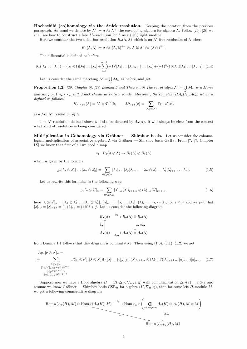
Suppose now we have a Hopf algebra H = (H,∆H ,∇H , ε, η) with comultiplication ∆H(x) = x ⊗ x andassume we know Grobner — Shirshov basis GSBH for algebra (H,∇H , η), then for some left H-module M ,we get a following commutative diagram

HomH(Ap(H),M)⊗HomH(Aq(H),M)

∨//

^

++

HomH⊗H

( ⊕r+s=p+q

Ar(H)⊗As(H),M ⊗M

)∆∗H

HomH(Ap+q(H),M)

4

where∨

-product [7, §7, Chapter IX] is given by the following formulae,

(ϑ∨ϑ′)(c⊗ c′) := ϑ(c)⊗ ϑ′(c′),

then using (1.7) we can describe ^-multiplication by the following formulae

(ϑp ^ ϑq)([v]p+q) =∑[λ⊗λ′]n∈(Λ⊗Λ)⊗n+1

[v]p∈V(p−1),

[u]q∈Vq−1

Γ([ν ⊗ ν′], [λ⊗ λ′])Γ([λ]1,p, [v]p)ϑp ([v]p) (λ′)p+1,p+q(λ)1,pΓ([λ′]p+1,q, [u]q)ϑq ([u]q) (1.8)

Remark 1.1. Since the comultiplication ∆(x) = x⊗ x is cocommutative, then ϑp ^ ϑq = (−1)pqϑq ^ ϑp,it can allow to simplify the (1.8).

2 The Plactic Monoid with Column Generators

In this section, we present an elegant algorithm proposed by C. Schensted. We will also see that there issome connection between Schensted’s column algorithm and braids.

Definition 2.1. Let A = 1, 2, . . . , n with 1 < 2 < · · · < n. Then we call Pl(A) := A∗/ ≡ the placticmonoid on the alphabet set A, where A∗ is the free monoid generated by A, ≡ is the congruence of A∗

generated by Knuth relations Ω and Ω consists of

ikj = kij (i ≤ j < k), jki = jik (i < j ≤ k).

For a field k, denote by kPl(A) or by kPln the plactic monoid algebra over k of Pl(A).

Definition 2.2. A strictly decreasing word w ∈ A∗ is called a column. Denote the set of columns by I.Let a ∈ I be a column and ai the number of the letter i in a. Then ai ∈ 0, 1, i = 1, 2, . . . , n. Puta = (a1; . . . ; an). Also we will consider any column as an ordered set a := ai1 , . . . , ai`, here aij = ∅iff aij = 0 and we will denote it by a = ei1,...,i` . Denote by e∅ the empty column (the unity of the placticmonoid).

For example, the word a = 875421 is a column, and we have a = (1; 1; 0; 1; 1; 0; 1; 1; 0; . . . ; 0), a =ai1 , ai2 , ai3 , ai4 , ai5 , ai6.

Definition 2.3 (Schensted’s column algorithm). Let a ∈ I be a column and let x ∈ A.

x · a =

xa, if xa is a column;

a′ · y, otherwise

where y is the rightmost letter in a and is larger than or equal to x, and a′ is obtained from a by replacingy with x. We say that an element y is connected to x or simply that elements y, x are connected. And wewill use the notation

x y :=

1, iff x is connected to y,

0, otherwise.

Definition 2.4. Consider two columns a, b ∈ I as ordered sets a, b and consider the columns

ba := x ∈ b : (y x) = 0 for any y ∈ a,

ba := x ∈ b : (y x) = 1 for some y ∈ a.Introduce binary operations ∨,∧ : I × I → I by the formulas:

a ∨ b := a ∪ ba, a ∧ b := ba,

then from Schensted’s column algorithm it follows that a · b = (a ∨ b) · (a ∧ b).

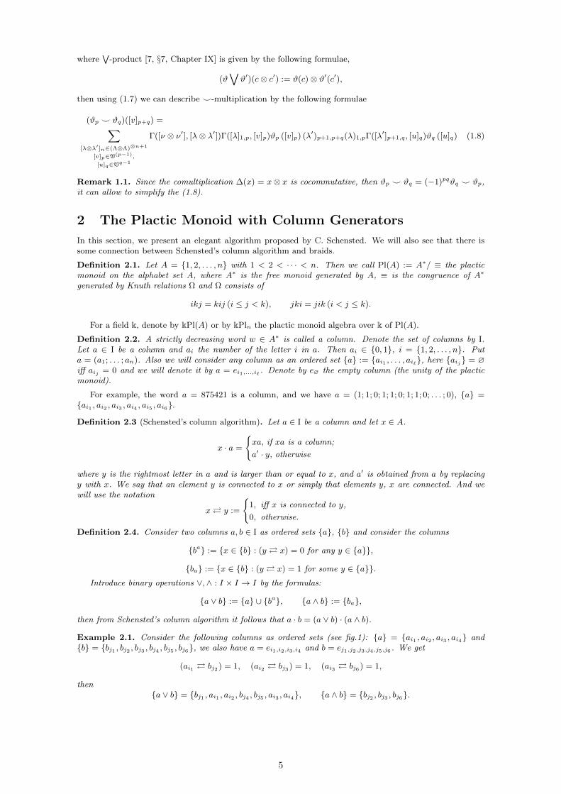
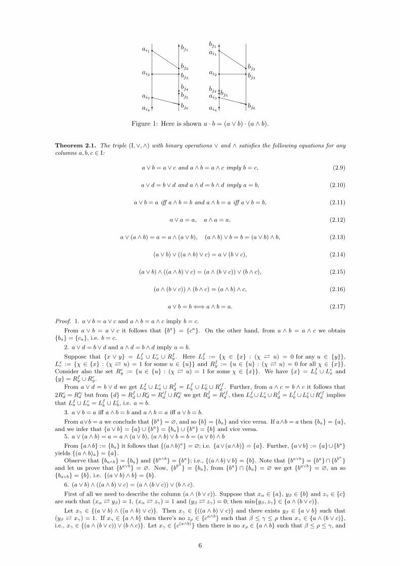
Example 2.1. Consider the following columns as ordered sets (see fig.1): a = ai1 , ai2 , ai3 , ai4 andb = bj1 , bj2 , bj3 , bj4 , bj5 , bj6, we also have a = ei1,i2,i3,i4 and b = ej1,j2,j3,j4,j5,j6 . We get

(ai1 bj2) = 1, (ai2 bj3) = 1, (ai3 bj6) = 1,

thena ∨ b = bj1 , ai1 , ai2 , bj4 , bj5 , ai3 , ai4, a ∧ b = bj2 , bj3 , bj6.

5

qai3 qbj6XXXXX

qai1qbj1

QQQQqbj2qai2 qbj3qbj4q

bj5qai4

qai2 bj3

ai3 qbj6XXXXX

qai1

qbj1Q

QQ

Qqbj2q qqbj4 qbj5qai4

Figure 1: Here is shown a · b = (a ∨ b) · (a ∧ b).

Theorem 2.1. The triple (I,∨,∧) with binary operations ∨ and ∧ satisfies the following equations for anycolumns a, b, c ∈ I:

a ∨ b = a ∨ c and a ∧ b = a ∧ c imply b = c, (2.9)

a ∨ d = b ∨ d and a ∧ d = b ∧ d imply a = b, (2.10)

a ∨ b = a iff a ∧ b = b and a ∧ b = a iff a ∨ b = b, (2.11)

a ∨ a = a, a ∧ a = a, (2.12)

a ∨ (a ∧ b) = a = a ∧ (a ∨ b), (a ∧ b) ∨ b = b = (a ∨ b) ∧ b, (2.13)

(a ∨ b) ∨ ((a ∧ b) ∨ c) = a ∨ (b ∨ c), (2.14)

(a ∨ b) ∧ ((a ∧ b) ∨ c) = (a ∧ (b ∨ c)) ∨ (b ∧ c), (2.15)

(a ∧ (b ∨ c)) ∧ (b ∧ c) = (a ∧ b) ∧ c, (2.16)

a ∨ b = b⇐⇒ a ∧ b = a. (2.17)

Proof. 1. a ∨ b = a ∨ c and a ∧ b = a ∧ c imply b = c.

From a ∨ b = a ∨ c it follows that ba = ca. On the other hand, from a ∧ b = a ∧ c we obtainba = ca, i.e. b = c.

2. a ∨ d = b ∨ d and a ∧ d = b ∧ d imply a = b.

Suppose that x ∨ y = Lfx ∪ Lcx ∪ Rfy . Here Lfx := χ ∈ x : (χ u) = 0 for any u ∈ y,Lxc := χ ∈ x : (χ u) = 1 for some u ∈ u and Rfy := u ∈ u : (χ u) = 0 for all χ ∈ x.Consider also the set Rcy := u ∈ u : (χ u) = 1 for some χ ∈ x. We have x = Lfx ∪ Lcx andy = Rfy ∪Rcy.

From a ∨ d = b ∨ d we get Lfa ∪ Lca ∪ Rfd = Lfb ∪ Lcb ∪ R′fd . Further, from a ∧ c = b ∧ c it follows that

2Rcd = R′cd but from d = Rfd ∪Rcd = R′fd ∪R

′cd we get Rfd = R′fd , then Lfa ∪Lca ∪Rfd = Lfb ∪L

cb ∪R′fd implies

that Lfa ∪ Lca = Lfb ∪ Lcb, i.e. a = b.

3. a ∨ b = a iff a ∧ b = b and a ∧ b = a iff a ∨ b = b.

From a∨b = a we conclude that ba = ∅, and so b = ba and vice versa. If a∧b = a then ba = a,and we infer that a ∨ b = a ∪ ba = ba ∪ ba = b and vice versa.

5. a ∨ (a ∧ b) = a = a ∧ (a ∨ b), (a ∧ b) ∨ b = b = (a ∨ b) ∧ bFrom a∧b := ba it follows that (a∧b)a = ∅; i.e. a∨ (a∧b) = a. Further, a∨b := a∪ba

yields (a ∧ b)a = a.Observe that ba∧b = ba and ba∧b = ba; i.e., (a∧ b)∨ b = b. Note that ba∨b = ba∩ bb

a

and let us prove that ba∨b = ∅. Now, bb

a

= ba, from ba ∩ ba = ∅ we get ba∨b = ∅, an soba∨b = b, i.e. (a ∨ b) ∧ b = b.

6. (a ∨ b) ∧ ((a ∧ b) ∨ c) = (a ∧ (b ∨ c)) ∨ (b ∧ c).First of all we need to describe the column (a ∧ (b ∨ c)). Suppose that xα ∈ a, yβ ∈ b and zγ ∈ c

are such that (xα yβ) = 1, (xα zγ) = 1 and (yβ zγ) = 0; then minyβ , zγ ∈ a ∧ (b ∨ c).Let xγ ∈ (a ∨ b) ∧ ((a ∧ b) ∨ c). Then xγ ∈ ((a ∧ b) ∨ c) and there exists yβ ∈ a ∨ b such that

(yβ xγ) = 1. If xγ ∈ a ∧ b then there’s no zρ ∈ ca∧b such that β ≤ γ ≤ ρ then xγ ∈ a ∧ (b ∨ c),i.e., xγ ∈ (a ∧ (b ∨ c)) ∨ (b ∧ c). Let xγ ∈ c(a∧b) then there is no xρ ∈ a ∧ b such that β ≤ ρ ≤ γ, and

6

hence xγ ∈ a ∧ (b ∨ c), i.e., xγ ∈ (a ∧ (b ∨ c)) ∨ (b ∧ c). We have proved that (a ∨ b) ∧ ((a ∧ b) ∨ c) ⊆(a ∧ (b ∨ c)) ∨ (b ∧ c).

Let xγ ∈ (a ∧ (b ∨ c)) ∨ (b ∧ c). If xγ ∈ (a ∧ (b ∨ c)) then xγ ∈ b ∨ c and there exists yα ∈ awith (yα xγ) = 1. Assume that xγ ∈ b. Then there is no zβ ∈ c such that α ≤ γ ≤ β. Therefore,xγ ∈ (a ∧ b) ∨ c. Since yα ∈ a, it follows that yα ∈ a ∨ b and, since (yα xγ) = 1, we see thatxγ ∈ (a ∨ b) ∧ ((a ∧ b) ∨ c). Suppose now that xγ ∈ cb. Then there is no zρ ∈ b with α ≤ ρ ≤ γ,and hence xγ ∈ (a ∧ b) ∨ c, and, since there is yα ∈ a, we get xγ ∈ (a ∨ b) ∧ ((a ∧ b) ∨ c). Now,consider the case xγ ∈ (b ∧ c). There exists zβ ∈ b such that (zβ xγ) = 1, and there is noyα ∈ a ∧ (b ∨ c) such that (yα xγ) = 1, i.e., if for some uρ ∈ a there exists xγ′ ∈ c with(uρ xγ′) = 1 then α ≤ γ′ < β; i.e., zβ ∈ ba, and hence xγ ∈ (a ∨ b) ∧ ((a ∧ b) ∨ c). We have provedthat (a ∨ b) ∧ ((a ∧ b) ∨ c) ⊇ (a ∧ (b ∨ c)) ∨ (b ∧ c).

7. (a ∧ (b ∨ c)) ∧ (b ∧ c) = (a ∧ b) ∧ c.Take cγ1 ∈ c and cγ1 ∈ (a∧(b∨c))∧(b∧c). Then there exists bβ1 ∈ b with (bβ1 cγ1) = 1 and also

there exists xcγ1∈ a∧ (b∨ c) such that (xcγ1

cγ1) = 1 and (xcγ1 bβ1) = 1. Since xcγ1

∈ a∧ (b∨ c),there exists yα ∈ a with (yα xcγ1

) = 1.Observe that if xcγ1

∈ b then (xcγ1 cγ1) = 1 and (bβ1 cγ1) = 1 but it is possible iff xcγ1

= bβ1 .This means that cγ1 ∈ c is connected with some xcγ1

∈ b which is connected with some yα ∈ a; i.e.,(a ∧ (b ∨ c)) ∧ (b ∧ c) ⊆ (a ∧ b) ∧ c.

If xcγ1∈ cb then γ1 ≤ β1 because (xcγ1

bβ1) = 1. This means there is no bβ2 ∈ b with α1 ≤ β2 ≤γ1; i.e., (bβ1 yα1) = 1, and hence (yα1 bβ1)(bβ1 cγ1) = 1; i.e., (a∧ (b∨ c))∧ (b∧ c) ⊆ (a∧ b)∧ c.

Let cγ1 ∈ (a ∧ b) ∧ c, i.e., cγ1 ∈ c and there exists bβ1 ∈ a ∧ b such that (bβ1 cγ1) = 1. Also forbβ1 there exists aα1 ∈ a such that (aα1 bβ1) = 1. Then cγ1 ∈ b ∧ c, and since (bβ1 cγ1) = 1, wemay assume that aα1 ∈ a ∧ (b ∨ c), i.e., (a ∧ b) ∧ c ⊆ (a ∧ (b ∨ c)) ∧ (b ∧ c)

8. (a ∨ b) ∨ ((a ∧ b) ∨ c) = a ∨ (b ∨ c).Is not hard to see that a ∨ (b ∨ c) = a ∪ (b ∨ c)a = a ∪ ba ∪ (cb)a because b ∧ cb = e∅. Then

we get (a ∨ b) ∨ ((a ∧ b) ∨ c) = a ∪ ba ∪ ((a ∧ b) ∨ c)(a∨b) = a ∪ ba ∪ (a ∧ b)(a∨b) ∪ c(a∨b) =a ∪ ba ∪ c(a∨b), but c(a∨b) = (cb)a; i.e., (a ∨ b) ∨ ((a ∧ b) ∨ c) = a ∨ (b ∨ c); as claimed.

9.a ∨ b = b⇐⇒ a ∧ b = a

Indeed, since a ∨ b := a ∪ ba and b = ba ∪ ba, it follows from a ∨ b = b that a = ba.

Suppose that a = (a1; . . . ; an) ∈ I and wt(a) := (a1 + . . . + an, a1, . . . , an). Order I as follows: for anya, b ∈ I, we say that a < b whenever wt(a) > wt(b) lexicographically. Then order I∗ by the deg-lex order.

Remark 2.1. Let a, b ∈ I. Then Schensted’s column algorithm and Definition 2.4 imply that a · b is theleading term iff a ∨ b 6= a and a ∧ b 6= b.

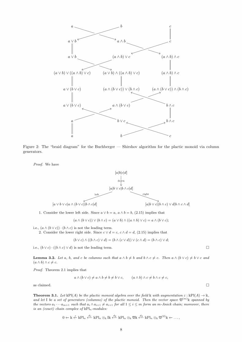
Remark 2.2. Put I := a ·b = (a∨b) ·(a∧b) : a, b ∈ I. Then we may assume [5] that k〈I〉/(I) ∼= k〈A〉/(Ω).Then formulas (3.6), (3.7), (3.8) enable us to prove that I is the Grobner — Shirshov basis of the placticmonoid in column generators (see also [5, Theorem 4.3]). In fig. 2, we show a sketch of the Buchberger —Shirshov algorithm for the plactic monoid via the binary operations ∨ and ∧. In the knot theory spirit, wecan interpret this operation as “overcrossing” and “udercrossing”.

Remark 2.3. The operations ∨, ∧ are not associative. Indeed, suppose that a = ei, b = ej and c = ek.Assume that j < k < i. Then (ei ∨ ej) ∨ ek = eji ∨ ek = ejiek. But ei ∨ (ej ∨ ek) = ei ∨ ek = eik; i.e.,

(a ∨ b) ∨ c 6= a ∨ (b ∨ c).

Assume now that j < i < k. Then (ei∧ej)∧ek = e∅∧ek = e∅. On other hand, ei∧(ej∧ek) = ei∧ek = ek;i.e.,

(a ∧ b) ∧ c 6= a ∧ (b ∧ c).However, we will use the notation a ∨ (b ∨ c) := a ∨ b ∨ c and (a ∧ b) ∧ c := a ∧ b ∧ c.

3 The Anick Resolution via Column Generators

Here we describe the Anick resolution for the kPln-module k and for the kPlen = kPln⊗k kPln-module kPln.

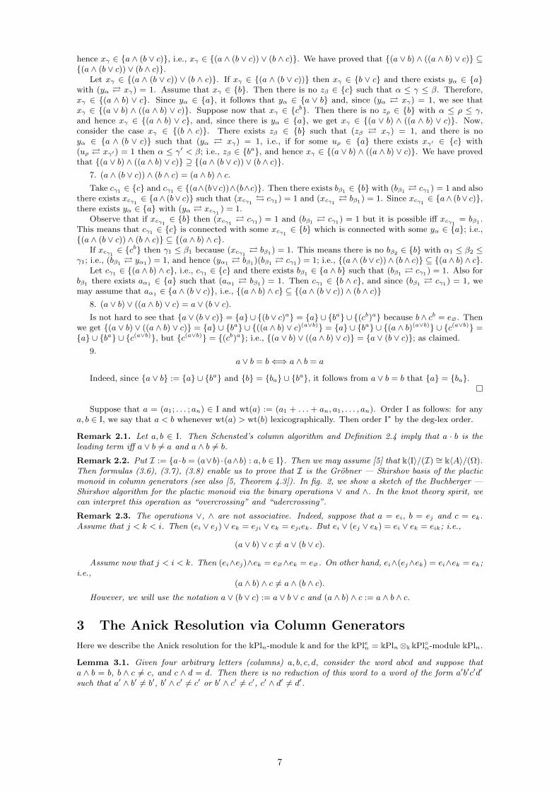
Lemma 3.1. Given four arbitrary letters (columns) a, b, c, d, consider the word abcd and suppose thata ∧ b = b, b ∧ c 6= c, and c ∧ d = d. Then there is no reduction of this word to a word of the form a′b′c′d′

such that a′ ∧ b′ 6= b′, b′ ∧ c′ 6= c′ or b′ ∧ c′ 6= c′, c′ ∧ d′ 6= d′.

7

a

**

b

tt

c

a ∨ b a ∧ b

**

c

tt

a ∨ b

**

(a ∧ b) ∨ c

tt

(a ∧ b) ∧ c

(a ∨ b) ∨ ((a ∧ b) ∨ c) (a ∨ b) ∧ ((a ∧ b) ∨ c) (a ∧ b) ∧ c

a ∨ (b ∨ c) (a ∧ (b ∨ c)) ∨ (b ∧ c) (a ∧ (b ∨ c)) ∧ (b ∧ c)

a ∨ (b ∨ c) a ∧ (b ∨ c)

44

b ∧ c

jj

a

44

b ∨ c

jj

b ∧ c

a b

44

c

jj

Figure 2: The “braid diagram” for the Buchberger — Shirshov algorithm for the plactic monoid via columngenerators.

Proof. We have

[a|b|c|d]

down

[a|b ∨ c|b ∧ c|d]

right

**

left

tt

[a ∨ b ∨ c|a ∧ (b ∨ c)|b ∧ c|d] [a|b ∨ c|(b ∧ c) ∨ d|b ∧ c ∧ d]

1. Consider the lower left side. Since a ∨ b = a, a ∧ b = b, (2.15) implies that

(a ∧ (b ∨ c)) ∨ (b ∧ c) = (a ∨ b) ∧ ((a ∧ b) ∨ c) = a ∧ (b ∨ c);

i.e., (a ∧ (b ∨ c)) · (b ∧ c) is not the leading term.2. Consider the lower right side. Since c ∨ d = c, c ∧ d = d, (2.15) implies that

(b ∨ c) ∧ ((b ∧ c) ∨ d) = (b ∧ (c ∨ d)) ∨ (c ∧ d) = (b ∧ c) ∨ d;

i.e., (b ∨ c) · ((b ∧ c) ∨ d) is not the leading term.

Lemma 3.2. Let a, b, and c be columns such that a ∧ b 6= b and b ∧ c 6= c. Then a ∧ (b ∨ c) 6= b ∨ c and(a ∧ b) ∧ c 6= c.

Proof. Theorem 2.1 implies that

a ∧ (b ∨ c) 6= a ∧ b 6= b 6= b ∨ c, (a ∧ b) ∧ c 6= b ∧ c 6= c,

as claimed.

Theorem 3.1. Let kPl(A) be the plactic monoid algebra over the field k with augmentation ε : kPl(A)→ k,and let I be a set of generators (columns) of the plactic monoid. Then the vector space V(m)k spanned bythe vectors a1 · · · am+1 such that ai ∧ ai+1 6= ai+1 for all 1 ≤ i ≤ m form an m-Anick chain; moreover, thereis an (exact) chain complex of kPln-modules:

0←− k ε←− kPlnd1←− kPln ⊗k Ik d2←− kPln ⊗k Vk d3←− kPln ⊗k V

(2)k←− . . . ,

8

where

dn([a1| . . . |a`]) =

=

`−1∑i=0

(−1)i(a1 ∨ . . . ∨ ai+1)[Li] +∑j=1

(−1)jε(ai ∧ . . . ∧ a`)[Ri] +

`−1∑m=1

∑m+l+k≤`−1

(−1)l+kWm,l,k. (3.18)

Here, for 1 ≤ i, j ≤ `− 1,

[Li] =

0, iff aj ∨ aj+1 = aj ∨ (aj+1 ∨ aj+2) for some i ≤ j ≤ `− 2,

[a1 ∧ (a2 ∨ · · · ∨ ai+1)| . . . |ai−1 ∧ (ai ∨ ai+1)|ai ∧ ai+1|ai+2| . . . |a`], otherwise.(3.19)

[Ri] =

0, iff aj ∧ aj+1 = (aj ∧ aj+1) ∧ aj+2

[a1| . . . |ai−1|ai ∨ ai+1|(ai ∧ ai+1) ∨ ai+2| . . . |(ai ∧ · · · ∧ a`−1) ∨ an], otherwise.(3.20)

Here L0 = [a2| . . . |a`], R` = [a1| . . . |a`],

Wm,l,k =

=

[a1| . . . |am−1|bm| . . . |bm+l−1|bm+l ∨ cm+l+1|cm+l+2| . . . |cm+l+k|am+l+k+1| . . . |a`], iff bm+l ∧ cm+l+1 = 1Pln

0, otherwise,

here

bm+ι =

am ∨ am+1, if ι = 0

(am ∧ · · · ∧ am+ι) ∨ am+ι+1, if 1 ≤ ι ≤ l − 1

am ∧ · · · ∧ am+l, if ι = l

or

bm+ι = −

am ∨ · · · ∨ am+l+1, if ι = 0

am+ι−1 ∧ (am+ι ∨ · · · ∨ am+l), if 1 ≤ ι ≤ l − 1

am+l−1 ∧ am+l, if ι = l

cm+ν = −

am+l ∨ · · · ∨ am+l+k, if ν = l + 1

am+ν−1 ∧ (am+ν ∨ · · · ∨ am+l+k), if ν = l + t, 1 ≤ t < k

am+l+k−1 ∧ am+l+k, if ν = l + k

or

cm+ν =

am+l+1 ∨ am+l+2, if ν = l + 1

(am+l+1 ∧ · · · ∧ am+ν) ∨ am+ν+1, if ν = l + t, 1 < t < k

am+l+1 ∧ · · · ∧ am+l+k, if ν = l + k.

Proof. Since the Grobner — Shirshov basis of the plactic monoid via column generators is quadratic non-homogeneous, V(m) = a1 · · · am+1 : ai ∧ ai+1 6= ai+1, for all 1 ≤ i ≤ m, for any m > 1. Following [20], wewill use the bar notation [a1| . . . |a`+1] for an `th Anick chain.

Let [a1| . . . |a`] ∈ V(`−1) be an ` − 1-Anick chain. Theorem 1.2 and Proposition 1.1 tell us that first we

must find all weighted paths pi : [a1| . . . |a`]ωi−→ [b1| . . . |b`−1] such that [b1| . . . |b`−1] ∈ V(`−2).

We say that the n-tuple [a1| . . . |ai ∨ ai+1|ai ∧ ai+1| . . . |a`] has a hole at the point i. Lemma 3.2 impliesthat we can move this hole to the left or to the right in the following sense:

[a1| . . . |ai ∨ ai+1|ai ∧ ai+1| . . . |a`]→→ [a1| . . . |ai∨ai+1|(ai∧ai+1)∨ai+2|(ai∧ai+1)∧ai+2| . . . |a`] movement of the hole to the right by one step

movement of the hole to the left by one step [a1| . . . |ai ∨ ai+1|ai ∧ ai+1| . . . |a`]→→ [a1| . . . |ai−1 ∨ (ai ∨ ai+1)|ai−1 ∧ (ai ∨ ai+1)|ai ∧ ai+1| . . . |a`].

Lemma 3.1 implies that, for finding paths pi : [a1| . . . |a`]ωi−→ [b1| . . . |b`−1], where [b1| . . . |b`−1] ∈ V(`−2),

we cannot make more than one hole in the tuple [a1| . . . |a`]. Assume that (ai ∨ai+1)∨ ((ai ∧ai+1)∨ai+2) 6=ai ∨ ai+1 and (ai ∧ (ai+1 ∨ ai+2)) ∧ (ai+1 ∧ ai+2) 6= ai+1 ∧ ai+2 for any 1 ≤ i ≤ `− 2 Then all paths pi havethe form

Li : [a1| . . . |a`]→→ [a1 ∨ · · · ∨ ai+1|a1 ∧ (a2 ∨ · · · ∨ ai+1)|a2 ∧ (a3 ∨ · · · ∨ ai+1)| . . . |ai−1 ∧ (ai ∨ ai+1)|ai ∧ ai+1|ai+2| . . . |a`] ,

9

Ri : [a1| . . . |a`]→→ [a1| . . . |ai−1|ai ∨ ai+1|(ai ∧ ai+1) ∨ ai+2|(ai ∧ ai+1 ∧ ai+2) ∨ ai+3| . . . |(ai ∧ · · · an−1) ∨ a`|a1 ∧ · · · ∧ a`].

Since Γ([a1| . . . |a`]→ Li) = (−1)i and Γ([a1| . . . |a`]→ Ri) = (−1)`−i, (1.3) implies

Γ([a1| . . . |a`]→ Li → Li) = (−1)iε(a1 ∨ . . . ∨ ai+1), Γ([a1| . . . |a`]→ Ri → Ri) = (−1)i(ai ∧ . . . ∧ a`),

and Proposition 1.1 yields (3.18).

Now, suppose that, for some 0 ≤ i ≤ `, we have (ai ∨ ai+1) ∧ ((ai ∧ ai+1) ∨ ai+2) = ((ai ∧ ai+1) ∨ ai+2)or (ai ∧ (ai+1 ∨ ai+2)) ∧ (ai+1 ∧ ai+2) = ai+1 ∧ ai+2. Theorem 2.1 implies that

ai ∨ ai+1 = (ai ∨ ai+1) ∨ ((ai ∧ ai+1) ∨ ai+2) = ai ∨ (ai+1 ∨ ai+2),

ai+1 ∧ ai+2 = (ai ∧ (ai+1 ∨ ai+2)) ∧ (ai+1 ∧ ai+2) = (ai ∧ ai+1) ∧ ai+2,

and we must put Ri = 0 (respectively, Li = 0). Finally, assuming that there are equalities of the forma′ ∧ b′ = 1Pln , we infer that there are paths of the form Wm,l,k with weight (−1)l+k. This completes theproof.

Theorem 3.2. In the above notation, we obtain the (exact) chain complex of kPlen-modules

0←− kPlend0←− kPlen ⊗k Ik d1←− kPlen ⊗k Vk d2←− kPlen ⊗k V

(2)k←− . . . ,

where

dn([a1| . . . |a`]) =

=

`−1∑i=0

(−1)i((a1 ∨ . . . ∨ ai+1)⊗ 1)[Li] +∑j=1

(−1)j(1⊗ (aj ∧ . . . ∧ a`))[Rj ] +

`−1∑m=1

∑m+l+k≤`−1

(−1)l+kWm,l,k.

(3.21)

Proof. The proof is the same as that of Theorem 3.1 with the exception of weights. As in the proof ofTheorem 3.1, we can give an explicit description of the paths:

Li : [a1| . . . |a`]→→ [a1 ∨ · · · ∨ ai+1|a1 ∧ (a2 ∨ · · · ∨ ai+1)|a2 ∧ (a3 ∨ · · · ∨ ai+1)| . . . |ai−1 ∧ (ai ∨ ai+1)|ai ∧ ai+1|ai+2| . . . |a`] ,

Ri : [a1| . . . |a`]→→ [a1| . . . |ai−1|ai ∨ ai+1|(ai ∧ ai+1) ∨ ai+2|(ai ∧ ai+1 ∧ ai+2) ∨ ai+3| . . . |(ai ∧ · · · an−1) ∨ a`|a1 ∧ · · · ∧ a`].

It follows from (1.4)

Γ([a1| . . . |a`]→ Li → Li) = (−1)i(a1∨ . . .∨ai+1)⊗1, Γ([a1| . . . |a`]→ Ri → Ri) = (−1)i1⊗ (ai∧ . . .∧a`),

and Proposition 1.2 gives (3.21).

4 The Cohomology Ring of the Plactic Monoid Algebra

We will use the notations Li[a1| . . . |a`] = Li = (a1∧(a2∨· · ·∨ai+1)) · · · (ai−1∧(ai∨ai+1))(ai∧ai+1)(ai+2 · · · a`)and Ri[a1| . . . |a`] = Ri = ((a1 · · · ai−1)(ai∨ai+1)((ai∧ai+1)∨ai+2)((ai∧· · ·∧a`−1))∨an). Here 0 ≤ i ≤ `−1and 1 ≤ j ≤ `.Lemma 4.1. Let M be a kPln-module and let ξ ∈ Homk(Ik,M), ζ ∈ Homk(V

(`−1)k,M). Then ξ ^ ζ, ζ ^ξ ∈ Homk(V

(`)k,M) can be described by the formulas

(ξ ^ ζ)[a1| . . . |a`+1] =∑i=0

(−1)i(ξ[a1 ∨ · · · ∨ ai+1]ε(Li)

)((a1 ∨ · · · ∨ ai+1)ζ[Li]

), (4.22)

(ζ ^ ξ)[a1| . . . |a`+1] =

`+1∑j=1

(−1)`+1−j(ζ[Rj ]ε(aj ∧ · · · ∧ a`+1)

)(Rjξ[aj ∧ · · · ∧ a`+1]

). (4.23)

Proof. Indeed, from (1.7) follows that we need to find all paths p of forms,

V(`) 3 [a1| . . . |a`+1]→ [b1| . . . |b`] ∈ V(`−1)

but from construction of R, L (see (3.19), (3.20)) follows that p = R, L, and weights of this paths werefound in proof of Theorem 3.1. This completes the proof.

10

Lemma 4.2. Let B be a kPlen-module, and let α ∈ Homk(Ik, B), β ∈ Homk(V(`−1)k, B). Then α ^ β, β ^

α ∈ Homk(V(`)k, B) can be described by the formulas

(ξ ^ ζ)[a1| . . . |a`+1] =∑i=0

(−1)i(ξ[a1 ∨ · · · ∨ ai+1]Li

)((a1 ∨ · · · ∨ ai+1)ζ[Li]

), (4.24)

(ζ ^ ξ)[a1| . . . |a`+1] =

`+1∑j=1

(−1)`+1−j(ζ[Rj ](aj ∧ · · · ∧ a`+1)

)(Rjξ[aj ∧ · · · ∧ a`+1]

). (4.25)

Proof. The proof is the same as for the previous Lemma with the exception of weights. Arguing as in proofof Theorem 3.2, we complete the proof.

Lemma 4.3. In the above notation, from

`+1∑j=1

(−1)j [Rj ]⊗ [a1 ∧ · · · ∧ a`+1] =∑i=0

(−1)i+1[Li]⊗ [a1 ∨ · · · ∨ ai+1],

it follows that ab = ba for all a, b ∈ a1, . . . , a`+1.

Proof. We have(−1)j0 = (−1)1

aj0 ∧ · · · ∧ a`+1 = a1

[Rj0 ] = [L0]

,

(−1)j1 = (−1)2

aj1 ∧ · · · ∧ a`+1 = a1 ∨ a2

[Rj1 ] = [L1]

, . . . ,

(−1)j` = (−1)`

aj` ∧ · · · ∧ a`+1 = a1 ∨ · · · ∨ a`+1

[Rj` ] = [L`]

,

here, 1 ≤ j0 6= j1 6= j2 6= . . . 6= j` ≤ `, i.e.

(−1)j0 = (−1)1

aj0 ∧ · · · ∧ a`+1 = a1

a1 = a2

a2 = a3

a3 = a4

. . . . . . . . . . . . . . . . . . . . . . . . . . . .

aj0−1 = aj0aj0 ∨ aj0+1 = aj0+1

(aj0 ∧ aj0+1) ∨ aj0+2 = aj1+2

. . . . . . . . . . . . . . . . . . . . . . . . . . . .

(aj0 ∧ · · · ∧ a`) ∨ a`+1 = a`+1

,

(−1)j1 = (−1)2

aj1 ∧ · · · ∧ a`+1 = a1 ∨ a2

a1 = a1 ∧ a2

a2 = a3

a3 = a4

. . . . . . . . . . . . . . . . . . . . . . . . . . . . . .

aj1−1 = aj1aj1 ∨ aj1+1 = aj1+1

(aj1 ∧ aj1+1) ∨ aj1+2 = aj1++2

. . . . . . . . . . . . . . . . . . . . . . . . . . . . . .

(aj1 ∧ · · · ∧ a`) ∨ a`+1 = a`+1

, . . .

. . . ,

(−1)js = (−1)s+1

ajs ∧ · · · ∧ a`+1 = a1 ∨ · · · ∨ as+1

a1 = a1 ∧ (a2 ∨ · · · ∨ as+1)

a2 = a2 ∧ (a3 ∨ · · · ∨ as+1)

a3 = a3 ∧ (a4 ∨ · · · ∨ as+1)

. . . . . . . . . . . . . . . . . . . . . . . . . . . . . . . .

as = as ∧ as+1

as+1 = as+2

. . . . . . . . . . . . . . . . . . . . . . . . . . . . . . . .

ajs−1 = ajsajs ∨ ajs+1 = ajs+1

(ajs ∧ ajs+1) ∨ ajs+2 = ajs+2

. . . . . . . . . . . . . . . . . . . . . . . . . . . . . . . .

(ajs ∧ · · · ∧ a`) ∨ a`+1 = a`+1

, . . . ,

(−1)j` = (−1)`+1

aj` ∧ · · · ∧ a`+1 = a1 ∨ · · · ∨ a`+1

a1 = a1 ∧ (a2 ∨ · · · ∨ a`+1)

a2 = a2 ∧ (a3 ∨ · · · ∨ a`+1)

a3 = a3 ∧ (a4 ∨ · · · ∨ a`+1)

. . . . . . . . . . . . . . . . . . . . . . . . . . . . . . . . . . . . . . . . . . . .

aj`−1 = aj`−1 ∧ (aj` ∨ · · · ∨ a`+1)

aj` ∨ aj`+1 = aj` ∧ (aj`+1 ∨ · · · ∨ a`+1)

(aj` ∧ aj`+1) ∨ aj`+2 = aj`+2 ∧ (aj`+3 ∨ a`+1)

. . . . . . . . . . . . . . . . . . . . . . . . . . . . . . . . . . . . . . . . . . . .

(aj` ∧ · · · ∧ a`) ∨ a`+1 = a` ∧ a`+1

.

It is not hard to see that this system has a nontrivial solution iff there is no relation of the form as = as+1,but it is possible iff

[R`+1] = [L`], [R`] = [L`−1], [R`−1] = [L`−2], . . . , [R1] = [L0]

11

i.e., we get

a1 = a1 ∧ (a2 ∨ · · · ∨ a`+1)

a2 = a2 ∧ (a3 ∨ · · · ∨ a`+1)

. . . . . . . . . . . . . . . . . . . . . . . . . .

a` = a` ∧ a`+1

a`+1 = a1 ∨ · · · ∨ a`+1

,

a1 = a1 ∧ (a2 ∨ · · · ∨ a`)a2 = a2 ∧ (a3 ∨ · · · ∨ a`). . . . . . . . . . . . . . . . . . . . . . .

a`−1 = a`−1 ∧ a`a` ∨ a`+1 = a`+1

a` ∧ a`+1 = a1 ∨ · · · ∨ a`

,

. . . ,

a1 = a1 ∧ (a2 ∨ · · · ∨ a`−s)a2 = a2 ∧ (a3 ∨ · · · ∨ a`−s). . . . . . . . . . . . . . . . . . . . . . . . . . . . . . . . . .

a`−s−1 = a`−s−1 ∧ a`−sa`−s ∨ a`−s+1 = a`−s+1

(a`−s ∧ a`−s+1) ∨ a`−s+2 = a`−s+2

. . . . . . . . . . . . . . . . . . . . . . . . . . . . . . . . . .

(a`−s ∧ · · · ∧ a`) ∨ a`+1 = a`+1

a`−s ∧ · · · ∧ a`+1 = a1 ∨ · · · ∨ a`−s

, . . . ,

a1 ∨ a2 = a2

(a1 ∧ a2) ∨ a3 = a3

. . . . . . . . . . . . . . . . . . . . . . . . . . .

(a1 ∧ · · · ∧ a`) ∨ a`+1 = a`+1

a1 ∧ · · · ∧ a`+1 = a1.

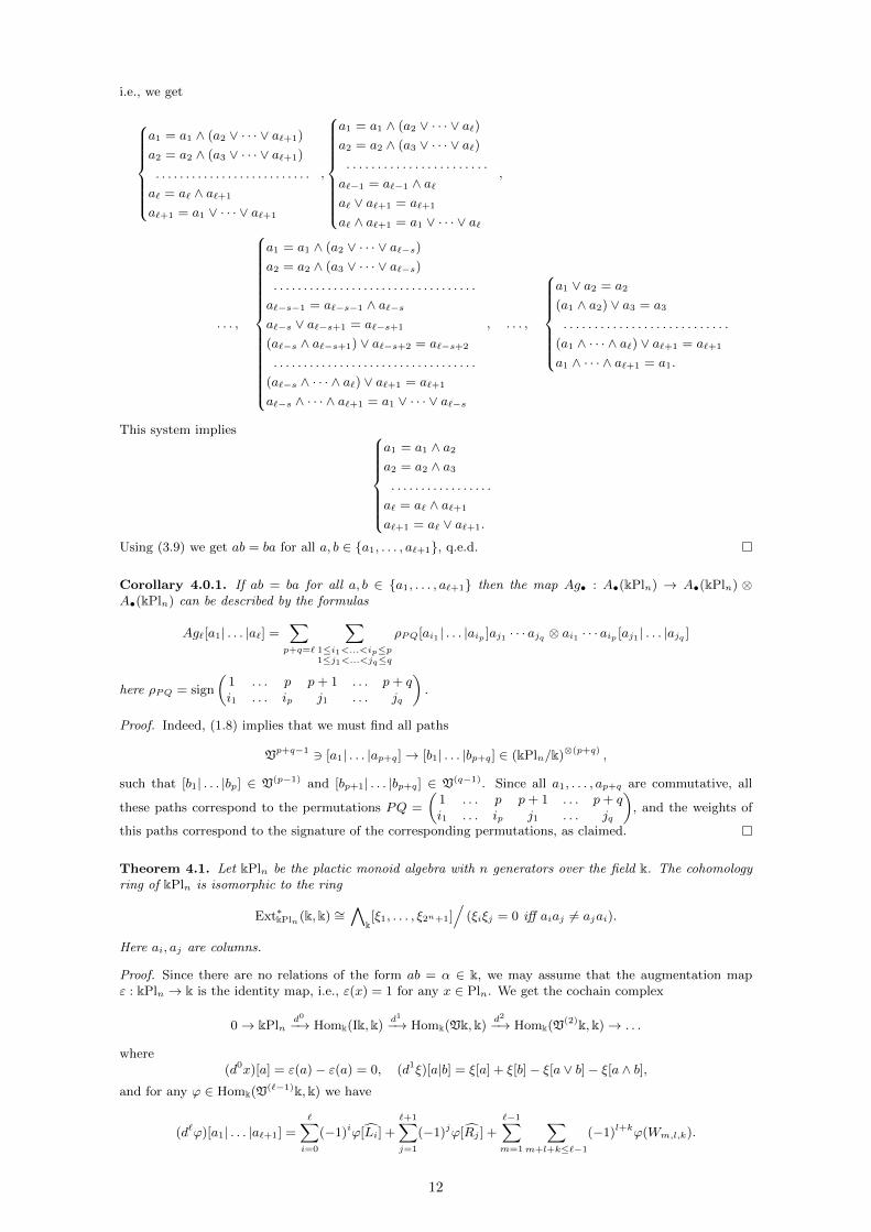
This system implies

a1 = a1 ∧ a2

a2 = a2 ∧ a3

. . . . . . . . . . . . . . . . .

a` = a` ∧ a`+1

a`+1 = a` ∨ a`+1.

Using (3.9) we get ab = ba for all a, b ∈ a1, . . . , a`+1, q.e.d.

Corollary 4.0.1. If ab = ba for all a, b ∈ a1, . . . , a`+1 then the map Ag• : A•(kPln) → A•(kPln) ⊗A•(kPln) can be described by the formulas

Ag`[a1| . . . |a`] =∑p+q=`

∑1≤i1<...<ip≤p1≤j1<...<jq≤q

ρPQ[ai1 | . . . |aip ]aj1 · · · ajq ⊗ ai1 · · · aip [aj1 | . . . |ajq ]

here ρPQ = sign

(1 . . . p p+ 1 . . . p+ qi1 . . . ip j1 . . . jq

).

Proof. Indeed, (1.8) implies that we must find all paths

Vp+q−1 3 [a1| . . . |ap+q]→ [b1| . . . |bp+q] ∈ (kPln/k)⊗(p+q) ,

such that [b1| . . . |bp] ∈ V(p−1) and [bp+1| . . . |bp+q] ∈ V(q−1). Since all a1, . . . , ap+q are commutative, all

these paths correspond to the permutations PQ =

(1 . . . p p+ 1 . . . p+ qi1 . . . ip j1 . . . jq

), and the weights of

this paths correspond to the signature of the corresponding permutations, as claimed.

Theorem 4.1. Let kPln be the plactic monoid algebra with n generators over the field k. The cohomologyring of kPln is isomorphic to the ring

Ext∗kPln(k, k) ∼=∧

k[ξ1, . . . , ξ2n+1]

/(ξiξj = 0 iff aiaj 6= ajai).

Here ai, aj are columns.

Proof. Since there are no relations of the form ab = α ∈ k, we may assume that the augmentation mapε : kPln → k is the identity map, i.e., ε(x) = 1 for any x ∈ Pln. We get the cochain complex

0→ kPlnd0

−→ Homk(Ik, k)d1

−→ Homk(Vk, k)d2

−→ Homk(V(2)k, k)→ . . .

where(d0x)[a] = ε(a)− ε(a) = 0, (d1ξ)[a|b] = ξ[a] + ξ[b]− ξ[a ∨ b]− ξ[a ∧ b],

and for any ϕ ∈ Homk(V(`−1)k, k) we have

(d`ϕ)[a1| . . . |a`+1] =∑i=0

(−1)iϕ[Li] +

`+1∑j=1

(−1)jϕ[Rj ] +

`−1∑m=1

∑m+l+k≤`−1

(−1)l+kϕ(Wm,l,k).

12

Consider the following functions:

ξa(x) =

1, if the column x has the form x = ex1,...,xr,a1,...,aα,xr+1,...,x` ,

0, otherwise,

here a = ea1,...,aα , x = ex1,...,x` ∈ I.Note that if ξa(x) = 1 and a ∧ x 6= x (i.e., it is an Anick chain) then ax = xa. Indeed, since x =

ex1,...,xr,a1,...,aα,xr+1,...,x` , we have x∨ a = x, and x∧ a = a, which wa required to prove. Also we infer thatξa is cocycle.

Let ϑp ∈ Homk(V(p−1)k, k) and let ϑq ∈ Homk(V

(q−1)k, k). Since the comultiplication kPln ⊗ kPln ←kPln : ∆(x) = x ⊗ x is cocomutative, then the product ^ must be skew commutative, i.e. (ϑp ^ ϑq) =(−1)pq(ϑq ^ ϑp). Consider the commutative diagram

Homk(V(p−1)k, k)⊗Homk(V

(q−1)k, k)^ //

τ∗

Homk(V(p+q−1)k, k)

τ

Homk(V(q−1)k, k)⊗Homk(V

(p−1)k, k) ^// Homk(V

(p+q−1)k, k).

Here τ : A•(kPln, k) ⊗ A•(kPln, k) → A•(kPln, k) ⊗ A•(kPln, k) is the chain automorphism such thatτ : x⊗ y → (−1)deg(x)deg(y)y ⊗ x.

We may assume without loss of generality that p = 1 and q = `. Suppose that ξ ∈ Homk(Ik, k) andζ ∈ Homk(V

(`−1), k). Then ξ ^ ζ = (−1)`ζ ^ ξ. Using (4.22), we obtain

(ξ ^ ζ)[a1| . . . |a`+1]! (ξ∨ζ)

(∑i=0

(−1)i[a1 ∨ · · · ∨ ai+1]⊗ [Li]

)τ∗−→

τ∗−→ (−1)`(ζ∨ξ)

(∑i=0

(−1)iLi ⊗ [a1 ∨ · · · ∨ ai+1]

)! (−1)`(ζ ^ ξ)[a1| . . . |a`+1],

and (4.23) implies that

`+1∑j=1

(−1)j [Rj ]⊗ [a1 ∧ · · · ∧ a`+1] =∑i=0

(−1)i+1[Li]⊗ [a1 ∨ · · · ∨ ai+1].

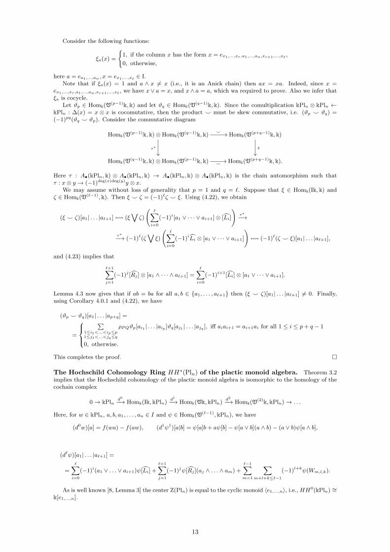
Lemma 4.3 now gives that if ab = ba for all a, b ∈ a1, . . . , a`+1 then (ξ ^ ζ)[a1| . . . |a`+1] 6= 0. Finally,using Corollary 4.0.1 and (4.22), we have

(ϑp ^ ϑq)[a1| . . . |ap+q] =

=

∑

1≤i1<...<ip≤p1≤j1<...<jq≤q

ρPQϑp[ai1 | . . . |aip ]ϑq[aj1 | . . . |ajq ], iff aiai+1 = ai+1ai for all 1 ≤ i ≤ p+ q − 1

0, otherwise.

This completes the proof.

The Hochschild Cohomology Ring HH∗(Pln) of the plactic monoid algebra. Theorem 3.2implies that the Hochschild cohomology of the plactic monoid algebra is isomorphic to the homology of thecochain complex

0→ kPlnd0

−→ Homk(Ik, kPln)d1

−→ Homk(Vk, kPln)d2

−→ Homk(V(2)k, kPln)→ . . .

Here, for w ∈ kPln, a, b, a1, . . . , an ∈ I and ψ ∈ Homk(V(`−1), kPln), we have

(d0w)[a] = f(wa)− f(aw), (d1ψ1)[a|b] = ψ[a]b+ aψ[b]− ψ[a ∨ b](a ∧ b)− (a ∨ b)ψ[a ∧ b],

(d`ψ)[a1| . . . |a`+1] =

=∑i=0

(−1)i(a1 ∨ . . . ∨ ai+1)ψ[Li] +

`+1∑j=1

(−1)jψ[Rj ](aj ∧ . . . ∧ am) +

`−1∑m=1

∑m+l+k≤`−1

(−1)l+kψ(Wm,l,k).

As is well known [8, Lemma 3] the center Z(Pln) is equal to the cyclic monoid 〈e1,...,n〉, i.e., HH0(kPln) ∼=k[e1,...,n].

13

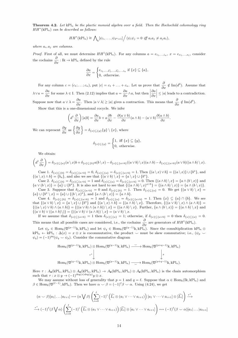
Theorem 4.2. Let kPln be the plactic monoid algebra over a field. Then the Hochschild cohomology ringHH∗(kPln) can be described as follows:

HH∗(kPln) ∼=∧

k[ψ1, . . . , ψ2n+1]

/(ψiψj = 0 iff aiaj 6= ajai),

where ai, aj are columns.

Proof. First of all, we must determine HH1(kPln). For any columns a = ei1,...,iα , x = ex1,...,x` , consider

the cochains∂

∂x: Ik→ kPln defined by the rule

∂a

∂x=

ei1,...,x1,...,x`,...,ia if x ⊆ a,0, otherwise.

For any column c = (c1; . . . ; cn), put |c| = c1 + . . . + cn. Let us prove that∂

∂x/∈ Im(d0). Assume that

λ∨a =∂a

∂xfor some λ ∈ I. Then (2.12) implies that a =

∂a

∂x∧a, but then

∣∣∣∣∂a∂x∣∣∣∣ ≤ |a| leads to a contradiction.

Suppose now that a ∨ λ =∂a

∂x. Then |a ∨ λ| ≥ |a| gives a contraction. This means that

∂

∂x/∈ Im(d0).

Show that this is a one-dimensional cocycle. We infer(d1 ∂

∂x

)[a|b] =

∂a

∂xb+ a

∂b

∂x− ∂(a ∨ b)

∂x(a ∧ b)− (a ∨ b)∂(a ∧ b)

∂x.

We can represent∂y

∂xas

∂y

∂x

= δx⊆yy \ x, where

δx⊆y =

1, iff x ⊆ y,0, otherwise.

We obtain:(d1 ∂

∂x

)= δx⊆a(a \ x)b+ δx⊆ba(b \ x)− δx⊆a∨b((a∨ b) \ x)(a∧ b)− δx⊆a∧b(a∨ b)((a∧ b) \ x).

Case 1. δx⊆b = δx⊆a∧b = 0, δx⊆a = δx⊆a∨b = 1. Then (a \x)∨ b = (a \x)∪ ba, and(a \ x) ∧ b = ba, and also we see that (a ∨ b) \ x = a \ x ∪ ba.

Case 2. δx⊆b = δx⊆a∧b = 1 and δx⊆a = δx⊆a∨b = 0. Then (a∧ b) \ x = a∧ (b \ x) anda ∨ (b \ x) = a ∪ ba. It is also not hard to see that ((a ∧ b) \ x)a∨b = (a ∧ b) \ x) = a ∧ (b \ x).

Case 3. Suppsoe that δx⊆a∧b = 0 and δx⊆b = 1. Then δx⊆a = 0. We get (a ∨ b) \ x =a ∪ ba \ x = a ∪ (b \ x)a, and a ∧ (b \ x) = a ∧ b.

Case 4. δx⊆b = δx⊆a∧b = 1 and δx⊆a = δx⊆a∨b = 1. Then x ⊆ a ∩ b. We seethat (a ∨ b) \ x = a \ x ∪ ba and (a \ x) ∧ b = (a ∧ b) \ x. Therefore, ((a ∨ b) \ x) ∧ (a ∧ b) =((a \ x) ∨ b) ∧ (a ∧ b) = ((a ∨ b) ∧ (a ∧ b)) \ x = (a ∧ b) \ x. Further, a ∧ (b \ x) = (a ∧ b) \ x and(a ∨ b) ∨ ((a ∧ b)\) = ((a ∨ b) ∨ (a ∧ b)) \ x = (a ∨ b) \ x.

If we assume that δx⊆a∨b = 1 then δx⊆a = 1; otherwise, if δx⊆a∨b = 0 then δx⊆a = 0.

This means that all possible cases are considered, i.e., the cochains∂

∂xare generators of HH1(kPln).

Let ψp ∈ Homk(V(p−1)k, kPln) and let ψq ∈ Homk(V

(q−1)k, kPln). Since the comultiplication kPln ⊗kPln ← kPln : ∆(x) = x ⊗ x is cocommutative, the product ^ must be skew commutative; i.e., (ψp ^ψq) = (−1)pq(ψq ^ ψp). Consider the commutative diagram

Homk(V(p−1)k, kPln)⊗Homk(V

(q−1)k, kPln)^ //

τ∗

Homk(V(p+q−1)k, kPln)

τ

Homk(V(q−1)k, kPln)⊗Homk(V

(p−1)k, kPln) ^// Homk(V

(p+q−1)k, kPln).

Here τ : A•(kPln, kPln) ⊗ A•(kPln, kPln) → A•(kPln, kPln) ⊗ A•(kPln, kPln) is the chain automorphismsuch that τ : x⊗ y → (−1)deg(x)deg(y)y ⊗ x.

We may assume without loss of generality that p = 1 and q = `. Suppose that α ∈ Homk(Ik, kPln) andβ ∈ Homk(V

(`−1), kPln). Then we have α ^ β = (−1)`β ^ α. Using (4.24), we get

(α ^ β)[a1| . . . |a`+1]! (α∨β)

(∑i=0

(−1)i(Li ⊗ (a1 ∨ · · · ∨ ai+1)

)[a1 ∨ · · · ∨ ai+1]⊗ [Li]

)τ∗−→

τ∗−→ (−1)`(β∨α)

(∑i=0

(−1)i(Li ⊗ (a1 ∨ · · · ∨ ai+1)

)[Li]⊗ [a1 ∨ · · · ∨ ai+1]

)! (−1)`(β ^ α)[a1| . . . |a`+1]

14

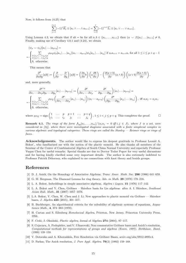
Now, it follows from (4.25) that

`+1∑j=1

(−1)jRj ⊗ [a1 ∧ · · · ∧ a`+1] =∑i=0

(−1)i+1Li ⊗ [a1 ∨ · · · ∨ ai+1].

Using Lemma 4.3, we obtain that if ab = ba for all a, b ∈ a1, . . . , a`+1 then (α ^ β)[a1| . . . |a`+1] 6= 0.Finally, making use of Corollary 4.0.1 and (4.24), we obtain

(ψp ^ ψq)[a1| . . . |ap+q] =

=

∑

1≤i1<...<ip≤p1≤j1<...<jq≤q

ρPQψp[ai1 | . . . |aip ](a1 · · · ap+q)ψq[aj1 | . . . |ajq ] if aiai+1 = ai+1ai for all 1 ≤ i ≤ p+ q − 1

0, otherwise.

This means that

∂2

∂x∂y[a|b] :=

(∂

∂x^

∂

∂y

)[a|b] =

(∂a

∂xb

)(a∂b

∂x

)−(∂(a ∨ b)∂x

(a ∧ b))(

(a ∨ b)∂(a ∧ b)∂x

),

and, more generally,

∂p+q

∂x1 · · · ∂xp∂y1 · · · ∂yq[a1| . . . |ap+q] :=

(∂p

∂x1 · · · ∂xp^

∂q

∂y1 · · · ∂yq

)[a1| . . . |ap+q] =

=

∑

1≤i1<...<ip≤p1≤j1<...<jq≤q

ρPQ

(∂p

∂x1 · · · ∂xp[ai1 | . . . |aip ]

)(a1 · · · ap+q)

(∂q

∂y1 · · · ∂yq[aj1 | . . . |ajq ]

), iff aiaj = ajai,

0, otherwise,

where ρPQ = sign

(1 . . . p p+ 1 . . . p+ qi1 . . . ip j1 . . . jq

), 1 ≤ i < j ≤ p+ q. This completes the proof.

Remark 4.1. The rings of the form∧R[α1, . . . , αm]

/(αiαj = 0 iff i, j ∈ J), where J is a set, were

considered in [24], where there were investigated diagrams associated with a finite simplicial complex invarious algebraic and topological categories. These rings are called the Stanley — Reisner rings or rings offaces.

Acknowledgements. The author would like to express his deepest gratitude to Professor Leonid A.Bokut’, who familiarized me with the notion of the plactic monoid. He also thanks all members of theSeminar of the Center of Combinatorial Algebra of South China Normal University and especially ProfessorYuqun Chen for useful remarks. Special thanks are due to Doctor Todor Popov for very useful discussionsand for having kindly clarified some very important details. The author is also extremely indebted toProfessor Patrick Dehornoy, who explained to me connections with knot theory and braids groups.

References

[1] D. J. Anick, On the Homology of Associative Algebras, Trans. Amer. Math. Soc. 296 (1986) 641–659.

[2] G. M. Bergman, The Diamond Lemma for ring theory, Adv. in Math. 29 (1978) 178–218.

[3] L. A. Bokut, Imbeddings in simple associative algebras, Algebra i Logica. 15 (1976) 117–142.

[4] L. A. Bokut and Y. Chen, Grobner – Shirshov basis for Lie algebras: after A. I. Shirshov, SoutheastAsian Bull. Math., 31 (2007) 1057–1076.

[5] L.A. Bokut, Y. Chen, W. Chen and J. Li, New approaches to plactic monoid via Grobner — Shirshovbases, J. Algebra 423 (2015), 301–317.

[6] B. Buchberger, An algorithmical criteria for the solvability of algebraic systems of equations, Aequa-tiones Math., 4, 374–383 (1970).

[7] H. Cartan and S. Eilenberg Homolocical Algebra, Priceton, New Jersey, Princeton University Press,1956.

[8] F. Cedo, J. Okninski, Plactic algebra, Jornal of Algebra 274 (2004), 97–117.

[9] S. Cojocaru, A. Podoplelov, and V. Ufnarovski, Non commutative Grobner bases and Anick’s resolution,Computational methods for representations of groups and algebras (Essen, 1997), Birkhause, Basel.(1999) 139–159.

[10] V. Dotsenko and A. Khoroshkin, Free Resolution via Grobner Bases, arxiv.org/abs/0912.4895v4.

[11] D. Farkas, The Anick resolution, J. Pure Appl. Algebra. 79(2) (1992) 159–168.

15

[12] M. Jollenbeck and V. Welke, Minimal Resolutions Via Algebraic Discrete Morse Theory, Mem. Am.Math. Soc. 197 (2009).

[13] H. Hironaka, Resolution of singularities of an algebraic variety over a field if characteristic zero, I, II,Ann. Math., 79 (1964) 109–203, 205–326.

[14] Y. Kobayashi, Complete rewriting systems and homology of monoid algebras, J. of Pure and Appl. Alg.65 (1990) 263–275.

[15] D.E. Knuth, Permutations, matrices, and generalized Young tabluaux, Pacific J. Math., 34, 709–727(1970).

[16] P. Malbos, Rewriting systems and Hochschild–Mitchell homology, Electr. Notes Theor. Comput. Sci.81 (2003) 59–72.

[17] Selected works of A. I. Shirshov, Eds. L. A. Bokut, V. Latyshev, I. Shestakov, E. Zelmanov, Trs. M.Bremmer, M. Kochetov, Birkhauser, Basel, Boston, Berlin, 2009

[18] R. Forman, Morse-Theory for cell-complexes, Adv. Math. 134 (1998) 90–145.

[19] R. Forman, A user’s guide to descrete Morse theory, Sem. Loth. de Comb. 48 (2002).

[20] M. Jollenbeck and V. Welke, Minimal Resolutions Via Algebraic Discrete Morse Theory, Mem. Am.Math. Soc. 197 (2009).

[21] A. Lascoux and M.P. Schutzenberger, Le monoide plaxique, in De Luca, A. (ED.), Non–CommutativeStructrures in Algebra and Geomtric Combinatorics, Vol. 109 of Quaderni de “La Ricerca Scientifica”,pp. 129–156. Consiglio Nazionale delle Ricerche, 1981.

[22] A. Lascoux, B. Leclerc and J.Y. Thibon, The plactic monoid, in: Algebraic Combinatorics on Words,Cambridge Univ. Press, 2002.

[23] J.-L. Loday, T. Popov, Parastatistics algebra, Young tableaux and the super plactic monoid Int. J.Geom. Meth. Mod. Phys. 5 (2008), 1295–1314.

[24] T. Panov, N. Ray, R. Vogt Colimits, Stanley–Reisner algebras, and loop spaces // Algebraic Topology:Categorical Decompostion Techniques, Progress in Math. V.215. Birkhauser, Basel, 2004. P.261–291;arXiv:math.AT/0202081.

[25] C. Schensted, Longest increasing and decrasing sub-seauances, Canad. J. Math., 13, 179–191 (1961).

[26] A.I. Shirshov, Some algorithmic problem for ε-algebras, Sibirsk. Math. Z., 3, 132–137 (1962).

[27] A. I. Shirshov, Some algorithm problems for Lie algebras, Sibirsk. Mat. Z. 3(2) 1962 292–296 (Russian);English translation in SIGSAM Bull. 33(2) (1999) 3–6.

[28] E. Skoldberg, Morse theory from an algebraic viewpoint, Trans. Amer. Math. Soc. 358(1) (2006) 115–129 (electronic).

[29] M. Dubouis – Viloette and T. Popov, Homogeneous Algebras, Statistics and Combinatorics, Lett MathPhys. 61(2), (2002), 159–170.

16