Stronger generalization bounds for deep nets via a compression

approach

Sanjeev Arora∗ Rong Ge† Behnam Neyshabur‡ Yi Zhang§

Abstract

Deep nets generalize well despite having more parameters than the number of training sam-ples. Recent works try to give an explanation using PAC-Bayes and Margin-based analyses, butdo not as yet result in sample complexity bounds better than naive parameter counting. Thecurrent paper shows generalization bounds that’re orders of magnitude better in practice. Theserely upon new succinct reparametrizations of the trained net — a compression that is explicitand efficient. These yield generalization bounds via a simple compression-based framework in-troduced here. Our results also provide some theoretical justification for widespread empiricalsuccess in compressing deep nets.

Analysis of correctness of our compression relies upon some newly identified “noise stabil-ity”properties of trained deep nets, which are also experimentally verified. The study of theseproperties and resulting generalization bounds are also extended to convolutional nets, whichhad eluded earlier attempts on proving generalization.

1 Introduction

A mystery about deep nets is that they generalize (i.e., predict well on unseen data) despite havingfar more parameters than the number of training samples. One commonly voiced explanation is thatregularization during training –whether implicit via use of SGD Neyshabur et al. [2015c], Hardt et al.[2016] or explicit via weight decay, dropout Srivastava et al. [2014], batch normalization Ioffe andSzegedy [2015], etc. –reduces the effective capacity of the net. But Zhang et al. [2017] questionedthis received wisdom and fueled research in this area by showing experimentally that standardarchitectures using SGD and regularization can still reach low training error on randomly labeledexamples (which clearly won’t generalize).

Clearly, deep nets trained on real-life data have some properties that reduce effective capacity,but identifying them has proved difficult —at least in a quantitative way that yields sample sizeupper bounds similar to classical analyses in simpler models such as SVMs Bartlett and Mendelson[2002], Evgeniou et al. [2000], Smola et al. [1998] or matrix factorization Fazel et al. [2001], Srebroet al. [2005].

Qualitatively Hochreiter and Schmidhuber [1997], Hinton and Van Camp [1993] suggested thatnets that generalize well are flat minima in the optimization landscape of the training loss and

∗Princeton University, Computer Science Department, email: arora@cs.princeton.edu†Duke University, Computer Science Department, email: rongge@cs.duke.edu‡Institute for Advanced Study, School of Mathematics, email: bneyshabur@ias.edu§Princeton University, Computer Science Department, email: y.zhang@cs.princeton.edu

1

arX

iv:1

802.

0529

6v4

[cs

.LG

] 2

6 N

ov 2

018

Hinton and Van Camp [1993] further discusses the connections to Minimum Description Lengthprinciple for generalization. Recently Keskar et al. [2016] show using experiments with differentbatch-sizes that sharp minima do correlate with higher generalization error. A quantitative versionof “flatness” was suggested in [Langford and Caruana, 2001]: the net’s output is stable to noiseadded to the net’s trainable parameters. Using PAC-Bayes bound [McAllester, 1998, 1999] thisnoise stability yielded generalization bounds for fully connected nets of depth 2. The theory hasbeen extended to multilayer fully connected nets [Neyshabur et al., 2017b], although thus faryields sample complexity bounds much worse than naive parameter counting. (Same holds for theearlier Bartlett and Mendelson [2002], Neyshabur et al. [2015b], Bartlett et al. [2017], Neyshaburet al. [2017a], Golowich et al. [2017]; see Figure 4). Another notion of noise stability —closelyrelated to dropout and batch normalization—is stability of the output with respect to the noiseinjected at the nodes of the network, which was recently shown experimentally [Morcos et al., 2018]to improve in tandem with generalization ability during training, and to be absent in nets trainedon random data. Chaudhari et al Chaudhari et al. [2016] suggest adding noise to gradient descentto bias it towards finding flat minima.

While study of generalization may appear a bit academic — held-out data easily establishesgeneralization in practice— the ultimate hope is that it will help identify simple, measurable andintuitive properties of well-trained deep nets, which in turn may fuel superior architectures andfaster training. We hope the detailed study —theoretical and empirical—in the current paperadvances this goal.Contributions of this paper.

1. A simple compression framework (Section 2) for proving generalization bounds, perhaps amore explicit and intuitive form of the PAC-Bayes work. It also yields elementary shortproofs of recent generalization results (Section 2.2).

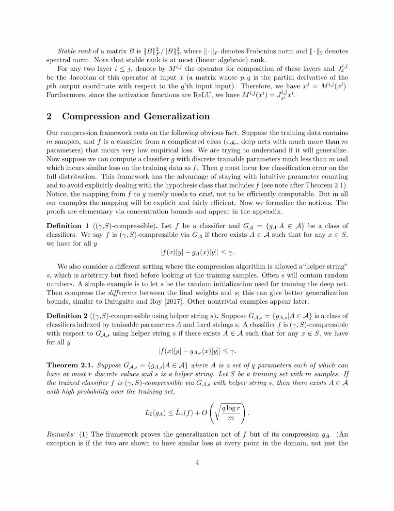
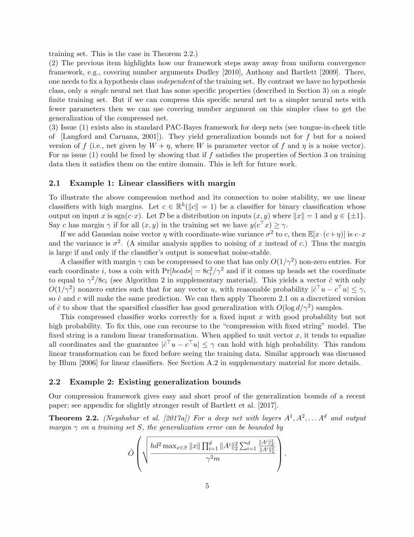
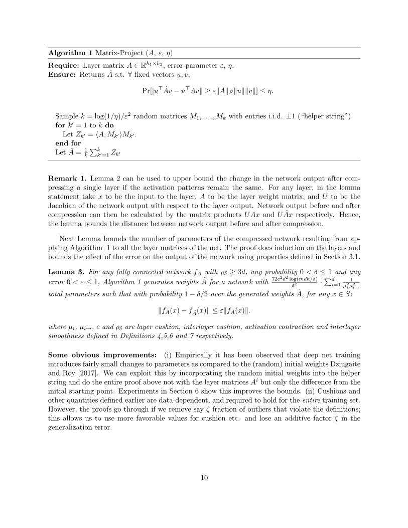
2. Identifying new form of noise-stability for deep nets: the stability of each layer’s computationto noise injected at lower layers. (Earlier papers worked only with stability of the output layer.)Figure 1 visualizes the stability of network w.r.t. Gaussian injected noise. Formal statementsrequire a string of other properties (Section 3). All are empirically studied, including theircorrelation with generalization (Section 6).

3. Using the above properties to derive efficient and provably correct algorithms that reduce theeffective number of parameters in the nets, yielding generalization bounds that: (a) are betterthan naive parameter counting (Section 6) (b) depend on simple, intuitive and measurableproperties of the network (Section 4) (c) apply also to convolutional nets (Section 5) (d)empirically correlate with generalization (Section 6).

The main idea is to show that noise stability allows individual layers to be compressed via alinear-algebraic procedure Algorithm 1. This results in new error in the output of the layer. Thisadded error is “gaussian-like” and tends to get attenuated as it propagates to higher layers.

Other related works. Dziugaite and Roy [2017] use non-convex optimization to optimize thePAC-Bayes bound get a non-vacuous sample bound on MNIST. While very creative, this provideslittle insight into favorable properties of networks. Liang et al. [2017] have suggested Fisher-Raometric, a regularization based on the Fisher matrix and showed that this metric correlate withgeneralization. Unfortunately, they could only apply their method to linear networks. RecentlyKawaguchi et al. [2017] connects Path-Norm Neyshabur et al. [2015a] to generalization. However,

2

0 1 2 3 4 5 6 7 8 9 10 11 12 13 14 15 16 17layer

0.00

0.02

0.04

0.06

0.08

0.10

erro

r ra

tiolayer 0layer 1layer 2layer 3layer 4layer 5layer 6layer 7layer 8layer 9layer 10

Figure 1: Attenuation of injected noise on a VGG-19 net trained on CIFAR-10. The x-axis is theindex of layers and y-axis denote the relative error due to the noise (‖xi − xi‖2/‖xi‖2). A curvestarts at the layer where a scaled Gaussian noise is injected to its input, whose `2 norm is set to10% of the norm of its original input. As it propagates up, the injected noise has rapidly decreasingeffect on higher layers. This property is shown to imply compressibility.

the proved generalization bound depends on the distribution and measuring it requires vectoroperations on exponentially high dimensional vectors. Other works have designed experiments toempirically evaluate potential properties of the network that helps generalizationArpit et al. [2017],Neyshabur et al. [2017b], Dinh et al. [2017]. The idea of compressing trained deep nets is verypopular for low-power applications; for a survey see [Cheng et al., 2018].

Finally, note that the terms compression and stability are traditionally used in a different sensein generalization theory Littlestone and Warmuth [1986], Kearns and Ron [1999], Shalev-Shwartzet al. [2010]. Our framework is compared to other notions in the remarks after Theorem 2.1.

Notation: We use standard formalization of multiclass classification, when data has to be assigneda label y of a sample x which is an integer from 1 to k. A multiclass classifier f maps input x to f(x) ∈Rk and the classification loss for any distribution D is defined as P(x,y)∼D [f(x)[y] ≤ maxi 6=y f(x)[j]] .If γ > 0 is some desired margin, then the expected margin loss is

Lγ(f) = P(x,y)∼D

[f(x)[y] ≤ γ + max

i 6=yf(x)[j]

](Notice, the classification loss corresponds to γ = 0.) Let Lγ denote empirical estimate of themargin loss. Generalization error is the difference between the two.

For most of the paper we assume that deep nets have fully connected layers, and use ReLUactivations. We treat convolutional nets in Section 5. If the net has d layers, we label the vectorbefore activation at these layers by x0, x1, xd for the d layers where x0 is the input to the net, alsodenoted simply x. So xi = Aiφ(xi−1) where Ai is the weight matrix of the ith layer. (Here φ(x) ifx is a vector applies the ReLU component-wise. The ReLU is allowed a trainable bias parameter,which is omitted from the notation because it has no effect on any calculations below.) We denotethe number of hidden units in layer i by hi and set h = maxdi=1 h

i. Let fA(x) be the functioncalculated by the above network.

3

Stable rank of a matrix B is ‖B‖2F /‖B‖22, where ‖ ·‖F denotes Frobenius norm and ‖ ·‖2 denotesspectral norm. Note that stable rank is at most (linear algebraic) rank.

For any two layer i ≤ j, denote by M i,j the operator for composition of these layers and J i,jxbe the Jacobian of this operator at input x (a matrix whose p, q is the partial derivative of thepth output coordinate with respect to the q’th input input). Therefore, we have xj = M i,j(xi).Furthermore, since the activation functions are ReLU, we have M i,j(xi) = J i,j

xixi.

2 Compression and Generalization

Our compression framework rests on the following obvious fact. Suppose the training data containsm samples, and f is a classifier from a complicated class (e.g., deep nets with much more than mparameters) that incurs very low empirical loss. We are trying to understand if it will generalize.Now suppose we can compute a classifier g with discrete trainable parameters much less than m andwhich incurs similar loss on the training data as f . Then g must incur low classification error on thefull distribution. This framework has the advantage of staying with intuitive parameter countingand to avoid explicitly dealing with the hypothesis class that includes f (see note after Theorem 2.1).Notice, the mapping from f to g merely needs to exist, not to be efficiently computable. But in allour examples the mapping will be explicit and fairly efficient. Now we formalize the notions. Theproofs are elementary via concentration bounds and appear in the appendix.

Definition 1 ((γ,S)-compressible). Let f be a classifier and GA = {gA|A ∈ A} be a class ofclassifiers. We say f is (γ, S)-compressible via GA if there exists A ∈ A such that for any x ∈ S,we have for all y

|f(x)[y]− gA(x)[y]| ≤ γ.

We also consider a different setting where the compression algorithm is allowed a“helper string”s, which is arbitrary but fixed before looking at the training samples. Often s will contain randomnumbers. A simple example is to let s be the random initialization used for training the deep net.Then compress the difference between the final weights and s; this can give better generalizationbounds, similar to Dziugaite and Roy [2017]. Other nontrivial examples appear later.

Definition 2 ((γ,S)-compressible using helper string s). Suppose GA,s = {gA,s|A ∈ A} is a class ofclassifiers indexed by trainable parameters A and fixed strings s. A classifier f is (γ, S)-compressiblewith respect to GA,s using helper string s if there exists A ∈ A such that for any x ∈ S, we havefor all y

|f(x)[y]− gA,s(x)[y]| ≤ γ.

Theorem 2.1. Suppose GA,s = {gA,s|A ∈ A} where A is a set of q parameters each of which canhave at most r discrete values and s is a helper string. Let S be a training set with m samples. Ifthe trained classifier f is (γ, S)-compressible via GA,s with helper string s, then there exists A ∈ Awith high probability over the training set,

L0(gA) ≤ Lγ(f) +O

(√q log r

m

).

Remarks: (1) The framework proves the generalization not of f but of its compression gA. (Anexception is if the two are shown to have similar loss at every point in the domain, not just the

4

training set. This is the case in Theorem 2.2.)(2) The previous item highlights how our framework steps away away from uniform convergenceframework, e.g., covering number arguments Dudley [2010], Anthony and Bartlett [2009]. There,one needs to fix a hypothesis class independent of the training set. By contrast we have no hypothesisclass, only a single neural net that has some specific properties (described in Section 3) on a singlefinite training set. But if we can compress this specific neural net to a simpler neural nets withfewer parameters then we can use covering number argument on this simpler class to get thegeneralization of the compressed net.(3) Issue (1) exists also in standard PAC-Bayes framework for deep nets (see tongue-in-cheek titleof [Langford and Caruana, 2001]). They yield generalization bounds not for f but for a noisedversion of f (i.e., net given by W + η, where W is parameter vector of f and η is a noise vector).For us issue (1) could be fixed by showing that if f satisfies the properties of Section 3 on trainingdata then it satisfies them on the entire domain. This is left for future work.

2.1 Example 1: Linear classifiers with margin

To illustrate the above compression method and its connection to noise stability, we use linearclassifiers with high margins. Let c ∈ Rh(‖c‖ = 1) be a classifier for binary classification whoseoutput on input x is sgn(c·x). Let D be a distribution on inputs (x, y) where ‖x‖ = 1 and y ∈ {±1}.Say c has margin γ if for all (x, y) in the training set we have y(c>x) ≥ γ.

If we add Gaussian noise vector η with coordinate-wise variance σ2 to c, then E[x ·(c+η)] is c ·xand the variance is σ2. (A similar analysis applies to noising of x instead of c.) Thus the marginis large if and only if the classifier’s output is somewhat noise-stable.

A classifier with margin γ can be compressed to one that has only O(1/γ2) non-zero entries. Foreach coordinate i, toss a coin with Pr[heads] = 8c2i /γ

2 and if it comes up heads set the coordinateto equal to γ2/8ci (see Algorithm 2 in supplementary material). This yields a vector c with onlyO(1/γ2) nonzero entries such that for any vector u, with reasonable probability |c>u − c>u| ≤ γ,so c and c will make the same prediction. We can then apply Theorem 2.1 on a discretized versionof c to show that the sparsified classifier has good generalization with O(log d/γ2) samples.

This compressed classifier works correctly for a fixed input x with good probability but nothigh probability. To fix this, one can recourse to the “compression with fixed string” model. Thefixed string is a random linear transformation. When applied to unit vector x, it tends to equalizeall coordinates and the guarantee |c>u − c>u| ≤ γ can hold with high probability. This randomlinear transformation can be fixed before seeing the training data. Similar approach was discussedby Blum [2006] for linear classifiers. See Section A.2 in supplementary material for more details.

2.2 Example 2: Existing generalization bounds

Our compression framework gives easy and short proof of the generalization bounds of a recentpaper; see appendix for slightly stronger result of Bartlett et al. [2017].

Theorem 2.2. (Neyshabur et al. [2017a]) For a deep net with layers A1, A2, . . . Ad and outputmargin γ on a training set S, the generalization error can be bounded by

O

√√√√hd2 maxx∈S ‖x‖

∏di=1 ‖Ai‖22

∑di=1

‖Ai‖2F‖Ai‖22

γ2m

.

5

The second part of this expression (∑d

i=1‖Ai‖2F‖Ai‖22

) is sum of stable ranks of the layers, a natural

measure of their true parameter count. The first part (∏di=1 ‖Ai‖22) is related to the Lipschitz

constant of the network, namely, the maximum norm of the vector it can produce if the input is aunit vector. The Lipschitz constant of a matrix operator B is just its spectral norm ‖B‖2. Since thenetwork applies a sequence of matrix operations interspersed with ReLU, and ReLU is 1-Lipschitzwe conclude that the Lipschitz constant of the full network is at most

∏di=1 ‖Ai‖2.

To prove Theorem 2.2 we use the following lemma to compress the matrix at each layer to amatrix of smaller rank. Since a matrix of rank r can be expressed as the product of two matrices ofinner dimension r, it has 2hr parameters (instead of the trivial h2). (Furthermore, the parameterscan be discretized via trivial rounding to get a compression with discrete parameters as needed byDefinition 1.)

Lemma 1. For any matrix A ∈ Rm×n, let A be the truncated version of A where singular valuesthat are smaller than δ‖A‖2 are removed. Then ‖A − A‖2 ≤ δ‖A‖2 and A has rank at most‖A‖2F /(δ2‖A‖22).

Proof. Let r be the rank of A. By construction, the maximum singular value of A − A is atmost δ‖A‖2. Since the remaining singular values are at least δ‖A‖2, we have ‖A‖F ≥ ‖A‖F ≥√rδ‖A‖2.

For each i replace layer i by its compression using the above lemma, with δ =γ(3‖x‖d∏d

i=1 ‖Ai‖2)−1. How much error does this introduce at each layer and how much doesit affect the output after passing through the intermediate layers (and getting magnified by their

Lipschitz constants)? Since A− Ai has spectral norm (i.e., Lipschitz constant) at most δ, the errorat the output due to changing layer i in isolation is at most δ‖xi‖∏d

j=1 ‖Aj‖2 ≤ γ/3d.A simple induction (see Neyshabur et al. [2017a] if needed) can now show the total error incurred

in all layers is bounded by γ. The generalization bound follows immediately from Theorem 2.1.

3 Noise stability properties of deep nets

This section introduces noise stability properties of deep nets that imply better compression (andhence generalization). They help overcome the pessimistic error analysis of our proof of Theo-rem 2.2: when a layer was compressed, the resulting error was assumed to blow up in a worst-casemanner according to the Lipschitz constant (namely, product of spectral norms of layers). Thishurt the amount of compression achievable. The new noise stability properties roughly amount tosaying that noise injected at a layer has very little effect on the higher layers. Our formalizationstarts with noise sensitivity, which captures how an operator transmits noise vs signal.

Definition 3. If M is a mapping from real-valued vectors to real-valued vectors, and N is somenoise distribution then noise sensitivity of M at x with respect to N , is

ψN (M,x) = Eη∈N[‖M(x+ η‖x‖)−M(x)‖2

‖M(x)‖2],

The noise sensitivity of M with respect to N on a set of inputs S, denoted ψN ,S(M), is the maximumof ψN (M,x) over all inputs x in S.

6

To illustrate, we examine noise sensitivity of a matrix (i.e., linear mapping) with respect toGaussian distribution. Low sensitivity turns out to imply that the matrix has some large singularvalues (i.e., low stable rank), which give directions that can preferentially carry the “signal”xwhereas noise η attenuates because it distributes uniformly across directions.

Proposition 3.1. The noise sensitivity of a matrix M at any vector x 6= 0 with respect to Gaussiandistribution N (0, I) is exactly ‖M‖2F ‖x‖2/‖Mx‖2, and at least its stable rank.

Proof. Using E[ηη>] = I, we bound the numerator by

Eη[‖M(x+ η‖x‖)−Mx‖2] = Eη[‖x‖2‖Mη‖2]

= Eη[‖x‖2tr(Mηη>M>)] = ‖x‖2tr(MM>) = ‖M‖2F ‖x‖2.

Thus noise sensitivity ψ at x is ‖M‖2F ‖x‖2/‖Mx‖2, which is at least the stable rank ‖M‖2F /‖M‖22since ‖Mx‖ ≤ ‖M‖2‖x‖.

The above proposition suggests that if a vector x is aligned to a matrix M (i.e. correlated withhigh singular directions of M), then matrix M becomes less sensitive to noise at x. This intuitionwill be helpful in understanding the properties we define later to formalize noise stability.

The above discussion motivates the following approach. We compress each layer i by an appro-priate randomized compression algorithm, such that the noise/error in its output is “Gaussian-like”.If layers i+ 1 and higher have low sensitivity to this new noise, then the compression can be moreextreme producing much higher noise. We formalize this idea using Jacobian J i,j , which describesinstantaneous change of M i,j(x) under infinitesimal perturbation of x.

3.1 Formalizing Error-resilience

Now we formalize the error-resilience properties. Section 6 reports empirical findings about theseproperties. The first is cushion, to be thought of roughly as reciprocal of noise sensitivity. We firstformalize it for single layer.

Definition 4 (layer cushion). The layer cushion of layer i is similarly defined to be the largestnumber µi such that for any x ∈ S, µi‖Ai‖F ‖φ(xi−1)‖ ≤ ‖Aiφ(xi−1)‖.

Intuitively, cushion considers how much smaller the output Aiφ(xi−1) is compared to the upperbound ‖Ai‖F ‖φ(xi−1)‖. Using argument similar to Proposition 3.1, we can see that 1/µ2i is equalto the noise sensitivity of matrix Ai at input φ(xi−1) with respect to Gaussian noise η ∼ N (0, I).

Of course, for nonlinear operators the definition of error resilience is less clean. Let’s denote byM i,j : Rhi → Rhj the operator corresponding to the portion of the deep net from layer i to layerj, and by J i,j its Jacobian. If infinitesimal noise is injected before level i then M i,j passes it likeJ i,j , a linear operator. When the noise is small but not infinitesimal then one hopes that M i,j stillbehaves roughly linearly (recall that ReLU nets are piecewise linear). To formalize this, we defineInterlayer Cushion (Definition 5) that captures the local linear approximation of the operator M .

Definition 5 (Interlayer Cushion). For any two layers i ≤ j, we define the interlayer cushion µi,jas the largest number such that for any x ∈ S:

µi,j‖J i,jxi ‖F ‖xi‖ ≤ ‖J i,j

xixi‖

7

Furthermore, for any layer i we define the minimal interlayer cushion as µi→ = mini≤j≤d µi,j =

min{1/√hi,mini<j≤d µi,j}1.

Since J i,jx is a linear transformation, a calculation similar to Proposition 3.1 shows that its noisesensitivity at xi with respect to Gaussian distribution N (0, I) is at most 1

µ2ij.

The next property quantifies the intuitive observation on the learned networks that for anytraining data, almost half of the ReLU activations at each layer are active. If the input to theactivations is well-distributed and the activations do not correlate with the magnitude of the input,then one would expect that on average, the effect of applying activations at any layer is to decreasethe norm of the pre-activation vector by at most some small constant factor.

Definition 6 (Activation Contraction). The activation contraction c is defined as the smallestnumber such that for any layer i and any x ∈ S,

‖φ(xi)‖ ≥ ‖xi‖/c.We discussed how the interlayer cushion captures noise-resilience of the network if it behaves

linearly, namely, when the set of activated ReLU gates does not change upon injecting noise. Ingeneral the activations do change, but the deviation from linear behavior is bounded for small noisevectors, as quantified next.

Definition 7 (Interlayer Smoothness). Let η be the noise generated as a result of substitutingweights in some of the layers before layer i using Algorithm 1. We define interlayer smoothness ρδto be the smallest number such that with probability 1 − δ over noise η for any two layers i < jany x ∈ S:

‖M i,j(xi + η)− J i,jxi

(xi + η)‖ ≤ ‖η‖‖xj‖

ρδ‖xi‖.

In order to understand the above condition, we can look at a single layer case where j = i+ 1:

‖M i,i+1(xi + η)− J i,i+1xi

(xi + η)‖ = ‖Ai+1φ(xi + η)−Ai+1(φ′(xi)� (xi + η))‖

= ‖Ai+1ν‖ ≤ ‖η‖‖Ai+1φ(xi)‖

ρδ‖xi‖where � is the entry-wise product operator and ν = (φ′(xi + η) − φ′(xi)) � (xi + η). Since theactivation function is ReLU, φ′(xi + η) and φ′(xi)) disagree whenever the perturbation has theopposite sign and higher absolute value compared to the input and hence ‖ν‖ ≤ ‖η‖.

Let us first see what happens if the perturbation ν is adversarially aligned to the weights:

‖M i,i+1(xi + η)− J i,i+1xi

(xi + η)‖

= ‖Ai+1ν‖ ≤ ‖Ai+1‖‖η‖ =‖η‖‖Ai+1φ(xi)‖

‖xi‖ · ‖Ai+1‖‖xi‖

‖Ai+1φ(xi)‖

≤ ‖η‖‖Ai+1φ(xi)‖‖xi‖ · ‖Ai+1‖‖xi‖

µi+1‖Ai+1‖F ‖φ(xi)‖ ≤‖η‖‖Ai+1φ(xi)‖

‖xi‖ · c‖Ai+1‖µi+1‖Ai+1‖F

=‖η‖‖Ai+1φ(xi)‖

‖xi‖ · c

µi+1ri+1

1Note that J i,ixi

= I and µi,i = 1/√hi

8

where ri+1 is the stable rank of layer i + 1. Therefore the interlayer smoothness from layer ito layer i + 1 is at least ρδ = µi+1ri+1/c. However, the noise generated from Algorithm 1 hassimilar properties to Gaussian noise (see Lemma 2). If ν behaves similar to Gaussian noise, then‖Ai+1ν‖ ≈ ‖Ai+1‖F ‖ν‖/

√hi and therefore ρδ is as high as

√hiµi+1/c. Since the layer cushion

of networks trained on real data is much more than that of networks with random weights, ρδ isgreater than one in this case. Another observation is that in practice, the noise is well-distributedand only a small portion of activations change from active to inactive and vice versa. Therefore,we can expect ‖ν‖ to be smaller than ‖η‖ which further improves the interlayer smoothness. This

appeared in Neyshabur et al. [2017b] that showed for one layer we can even use ‖η‖1.5‖xj‖ρδ‖xi‖

as the

RHS of interlayer smoothness. Our current proof requires 1/ρδ to be of order 1/d, this requirementcan be removed (with ρδ appear in sample complexity) if we make the stronger assumption thatthe RHS is a lower order term in ‖η‖.

In general, for a single layer, ρδ captures the ratio of input/weight alignment to noise/weightalignment. Since the noise behaves similar to Gaussian, one expects this number to be greaterthan one for a single layer. When j > i+ 1, the weights and activations create more dependencies.However, since these dependences are applied on both noise and input, we again expect that ifthe input is more aligned to the weights than noise, this should not change in higher layers. InSection 6, we show that the interlayer smoothness is indeed good: 1/ρδ is a small constant.

4 Fully Connected Networks

We prove generalization bounds using for fully connected multilayer nets. Details appear in Ap-pendix Section B.

Theorem 4.1. For any fully connected network fA with ρδ ≥ 3d, any probability 0 < δ ≤ 1 andany margin γ, Algorithm 1 generates weights A for the network fA such that with probability 1− δover the training set and fA, the expected error L0(fA) is bounded by

Lγ(fA) + O

√√√√c2d2 maxx∈S ‖fA(x)‖22

∑di=1

1µ2iµ

2i→

γ2m

where µi, µi→, c and ρδ are layer cushion, interlayer cushion, activation contraction and interlayersmoothness defined in Definitions 4,5,6 and 7 respectively.

To prove this we describe a compression of the net with respect to a fixed (random) string. Incontrast to the deterministic compression of Lemma 1, this randomized compression ensures thatthe resulting error in the output behaves like a Gaussian. The proofs are similar to standard JLdimension reduction.

Note that the helper string of random matrices Mi’s were chosen and fixed before training set Swas picked. Each weight matrix is thus represented as only k real numbers 〈A,Mi〉 for i = 1, 2, ..., k.

Lemma 2. For any 0 < δ, ε ≤ 1, et G = {(U i, xi)}mi=1 be a set of matrix/vector pairs of size mwhere U ∈ Rn×h1 and x ∈ Rh2, let A ∈ Rh1×h2 be the output of Algorithm 1 with η = δ/mn. Withprobability at least 1− δ we have for any (U, x) ∈ G, ‖U(A−A)x‖ ≤ ε‖A‖F ‖U‖F ‖x‖.

9

Algorithm 1 Matrix-Project (A, ε, η)

Require: Layer matrix A ∈ Rh1×h2 , error parameter ε, η.Ensure: Returns A s.t. ∀ fixed vectors u, v,

Pr[|u>Av − u>Av‖ ≥ ε‖A‖F ‖u‖‖v‖] ≤ η.

Sample k = log(1/η)/ε2 random matrices M1, . . . ,Mk with entries i.i.d. ±1 (“helper string”)for k′ = 1 to k do

Let Zk′ = 〈A,Mk′〉Mk′ .end forLet A = 1

k

∑kk′=1 Zk′

Remark 1. Lemma 2 can be used to upper bound the change in the network output after com-pressing a single layer if the activation patterns remain the same. For any layer, in the lemmastatement take x to be the input to the layer, A to be the layer weight matrix, and U to be theJacobian of the network output with respect to the layer output. Network output before and aftercompression can then be calculated by the matrix products UAx and UAx respectively. Hence,the lemma bounds the distance between network output before and after compression.

Next Lemma bounds the number of parameters of the compressed network resulting from ap-plying Algorithm 1 to all the layer matrices of the net. The proof does induction on the layers andbounds the effect of the error on the output of the network using properties defined in Section 3.1.

Lemma 3. For any fully connected network fA with ρδ ≥ 3d, any probability 0 < δ ≤ 1 and any

error 0 < ε ≤ 1, Algorithm 1 generates weights A for a network with 72c2d2 log(mdh/δ)ε2

·∑di=1

1µ2iµ

2i→

total parameters such that with probability 1− δ/2 over the generated weights A, for any x ∈ S:

‖fA(x)− fA(x)‖ ≤ ε‖fA(x)‖.

where µi, µi→, c and ρδ are layer cushion, interlayer cushion, activation contraction and interlayersmoothness defined in Definitions 4,5,6 and 7 respectively.

Some obvious improvements: (i) Empirically it has been observed that deep net trainingintroduces fairly small changes to parameters as compared to the (random) initial weights Dziugaiteand Roy [2017]. We can exploit this by incorporating the random initial weights into the helperstring and do the entire proof above not with the layer matrices Ai but only the difference from theinitial starting point. Experiments in Section 6 show this improves the bounds. (ii) Cushions andother quantities defined earlier are data-dependent, and required to hold for the entire training set.However, the proofs go through if we remove say ζ fraction of outliers that violate the definitions;this allows us to use more favorable values for cushion etc. and lose an additive factor ζ in thegeneralization error.

10

5 Convolutional Neural Networks

Now we sketch how to provably compress convolutional nets. (Details appear in Section C ofsupplementary.) Intuitively, this feels harder because the weights are already compressed— they’reshared across patches!

Theorem 5.1. For any convolutional neural network fA with ρδ ≥ 3d, any probability 0 < δ ≤ 1and any margin γ, Algorithm 4 generates weights A for the network fA such that with probability1− δ over the training set and fA:

L0(fA) ≤ Lγ(fA)

+ O

√√√√c2d2 maxx∈S ‖fA(x)‖22

∑di=1

β2(dκi/sie)2µ2iµ

2i→

γ2m

where µi, µi→, c, ρδ and β are layer cushion, interlayer cushion, activation contraction, inter-layer smoothness and well-distributed Jacobian defined in Definitions 4,8,6, 7 and 9 respectively.Furthermore, si and κi are stride and filter width in layer i.

Let’s realize that obvious extensions of earlier sections fail. Suppose layer i of the neural networkis an image of dimension ni1 × ni2 and each pixel has hi channels, the size of the filter at layer i isκi × κi with stride si. The convolutional filter has dimension hi−1 × hi × κi × κi. Applying matrixcompression (Algorithm 1) independently to each copy of a convolutional filter makes number ofnew parameters proportional to ni1n

i2, a big blowup.

Compressing a convolutional filter once and reusing it in all patches doesn’t work because theinterlayer analysis implicitly requires the noise generated by the compression to behave similar toa spherical Gaussian, but the shared filters introduce correlations. Quantitatively, using the fullyconnected analysis would require the error to be less than interlayer cushion value µi→ (Definition 5)

which is at most 1/√hini1n

i2, and this can never be achieved from compressing matrices that are

far smaller than ni1 × ni2 to begin with.We end up with a solution in between fully independent and fully dependent: p-wise indepen-

dence. The algorithm generates p-wise independent compressed filters A(a,b) for each convolutionlocation (a, b) ∈ [ni1] × [ni2]. It results in p times more parameters than a single compression. Ifp grows logarithmically with relevant parameters, the filters behave like fully independent filters.Using this idea we can generalize the definition of interlayer margin to the convolution setting:

Definition 8 (Interlayer Cushion, Convolution Setting). For any two layers i ≤ j, we define theinterlayer cushion µi,j as the largest number such that for any x ∈ S:

µi,j ·1√ni1n

i2

‖J i,jxi‖F ‖xi‖ ≤ ‖J i,jxi x

i‖

Furthermore, for any layer i we define the minimal interlayer cushion as µi→ = mini≤j≤d µi,j =

min{1/√hi,mini<j≤d µi,j}2.

2Note that J i,ixi

= I and µi,i = 1/√hi

11

Recall that interlayer cushion is related to the noise sensitivity of J i,jxi

at xi with respect to

Gaussian distribution N (0, I). When we consider J i,jxi

applied to a noise η, if different pixels in η

are independent Gaussians, then we can indeed expect ‖J i,jxiη‖ ≈ 1√

hini1ni2

‖J i,jxi‖‖η‖, which explains

the extra 1√ni1n

i2

factor in Definition 8 compared to Definition 5. The proof also needs to assume

—in line with intuition behind convolution architecture— that information from the entire imagefield is incorporated somewhat uniformly across pixels. It is formalized using the Jacobian whichgives the partial derivative of the output with respect to pixels at previous layer.

Definition 9 (Well-distributed Jacobian). Let J i,jx be the Jacobian of M i,j at x, we know J i,jx ∈Rhi×ni1×ni2×hj×n

j1×n

j2 . We say the Jacobian is β well-distributed if for any x ∈ S, any i, j, any

(a, b) ∈ [ni1 × ni2],‖[J i,jx ]:,a,b,:,:,:‖F ≤

β√ni1n

i2

‖J i,jx ‖F

6 Empirical Evaluation

We study noise stability properties (defined in Section 3) of an actual trained deep net, and computea generalization bound from Theorem 5.1. Experiments were performed by training a VGG-19architecture Simonyan and Zisserman [2014] and a AlexNet Krizhevsky et al. [2012] for multi-classclassification task on CIFAR-10 dataset. Optimization used SGD with mini-batch size 128, weightdecay 5e-4, momentum 0.9 and initial learning rate 0.05, but decayed by factor 2 every 30 epochs.Drop-out was used in fully-connected layers. We trained both networks for 299 epochs and thefinal VGG-19 network achieved 100% training and 92.45% validation accuracy while the AlexNetachieved 100% training and 77.22% validation accuracy. To investigate the effect of corruptedlabel, we trained another AlexNet, with 100% training and 9.86% validation accuracy, on CIFAR-10 dataset with randomly shuffled labels.

Our estimate of the sample complexity bound used exact computation of norms of weight matri-ces (or tensors) in all bounds(||A||1,∞, ||A||1,2, ||A||2, ||A||F ). Like previous bounds in generalizationtheory, ours also depend upon nuisance parameters like depth d, logarithm of h, etc. which prob-ably are an artifact of the proof. These are ignored in the computation (also in computing earlierbounds) for simplicity. Even the generalization based on parameter counting arguments does havean extra dependence on depth Bartlett et al. [2017]. A recent work, Golowich et al. [2017] showedthat many such depth dependencies can be improved.

6.1 Empirical investigation of noise stability properties

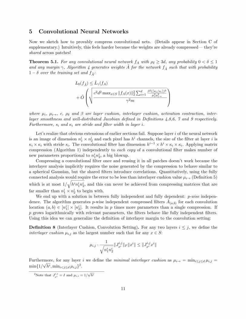
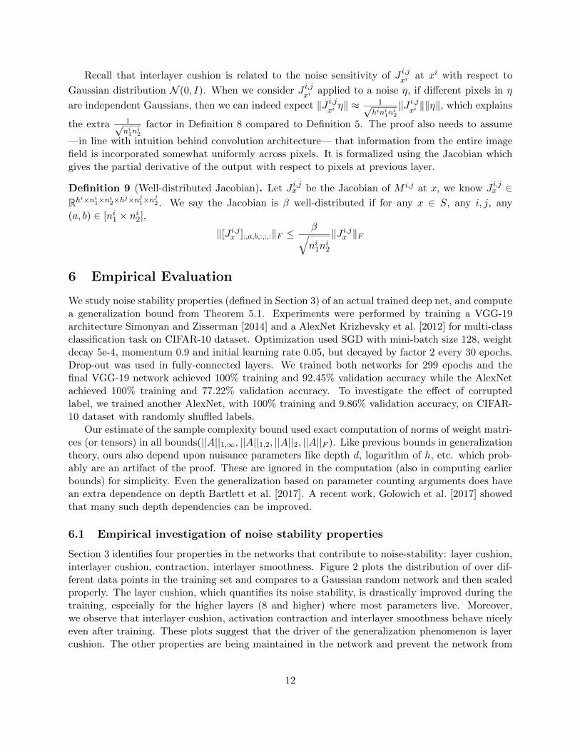
Section 3 identifies four properties in the networks that contribute to noise-stability: layer cushion,interlayer cushion, contraction, interlayer smoothness. Figure 2 plots the distribution of over dif-ferent data points in the training set and compares to a Gaussian random network and then scaledproperly. The layer cushion, which quantifies its noise stability, is drastically improved during thetraining, especially for the higher layers (8 and higher) where most parameters live. Moreover,we observe that interlayer cushion, activation contraction and interlayer smoothness behave nicelyeven after training. These plots suggest that the driver of the generalization phenomenon is layercushion. The other properties are being maintained in the network and prevent the network from

12

falling prey to pessimistic assumptions that causes the other older generalization bounds to bevery high. The assumptions made in section 3 (also in B.1) are verified on the VGG-19 net inappendix D.1 by histogramming the distribution of layer cushion, interlayer cushion, contraction,interlayer smoothness, and well-distributedness of the Jacobians of each layer of the net on eachdata point in the training set. Some examples are shown in Figure 2.

0.0 0.1 0.2 0.3a) layer cushion µi

random inittrained

0.2 0.4 0.6b) minimal inter-layer cushion µi!

random inittrained

1.0 1.2 1.4c) contraction c

random inittrained

0.00 0.02 0.04 0.06d) interlayer smoothness 1/⇢

random inittrained

Figure 2: Distribution of a) layer cushion, b) (unclipped) minimal interlayer cushion, c) activationcontraction and d) interlayer smoothness of the 13-th layer of VGG-19 nets on on training set. Thedistributions on a randomly-initialized and a trained net are shown in blue and orange. Note thatafter clipping, the minimal interlayer cushion is set to 1/

√hi for all layers except the first one, see

appendix D.1.

6.2 Correlation to generalization error

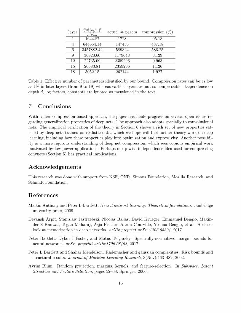
We evaluate our generalization bound during the training, see Figure 4, Right. After 120 epochs,the training error is almost zero but the test error continues to improve in later epochs. Ourgeneralization bound continues to improve, though not to the same level. Thus our generalizationbound captures part of generalization phenomenon, not all. Still, this suggests that SGD somehowimproves our generalization measure implicitly. Making this rigorous is a good topic for furtherresearch.

Furthermore, we investigate effect of training with normal data and corrupted data by trainingtwo AlexNets respectively on original and corrupted CIFAR-10 with randomly shuffled labels.We identify two key properties that differ significantly between the two networks: layer cushionand activation contraction, see 4. Since our bound predicts larger cushion and lower contractionindicates better generalization, our bound is consistent w with the fact that the net trained onnormal data generalizes (77.22% validation accuracy).

13

6.3 Comparison to other generalization bounds

Figure 4 compares our proposed bound to other neural-net generalization bounds on the VGG-19net and compares to naive VC dimension bound (which of course is too pessimistic). All previousgeneralization bounds are orders of magnitude worse than ours; the closest one is spectral normstimes average `1,2 of the layers Bartlett et al. [2017] which is still about 1015, far greater than VCdimension. (As mentioned we’re ignoring nuisance factors like depth and log h which make thecomparison to VC dimension a bit unfair, but the comparison to previous bounds is fair.) Thisshould not be surprising as all other bounds are based on product of norms which is pessimistic(see note at the start of Section 3) which we avoid due to the noise stability analysis.

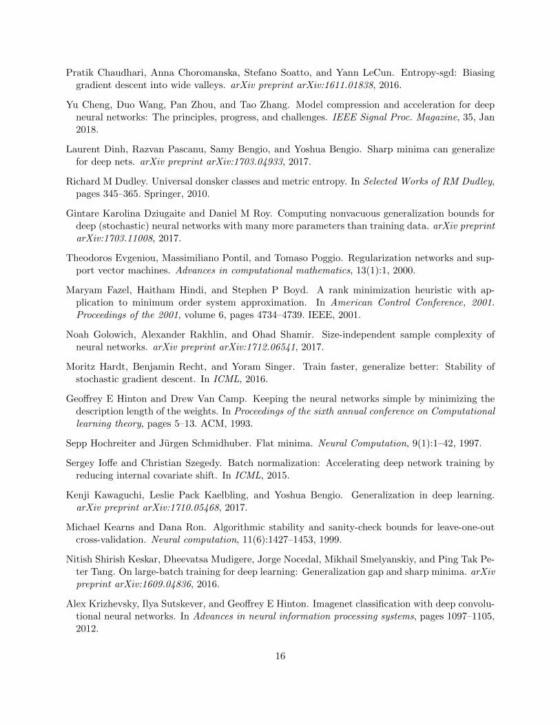
Table 1 shows the compressibility of various layers according to the bounds given by our theorem.Again, this is a qualitative due to ignoring nuisance factors, but it gives an idea of which layers areimportant in the calculation.

0.05 0.10 0.15a) layer cushion i

normalcorrupted

1.0 1.5 2.0 2.5b) contraction c

normalcorrupted

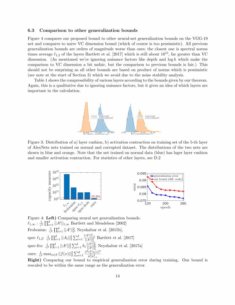
Figure 3: Distribution of a) layer cushion, b) activation contraction on training set of the 5-th layerof AlexNets nets trained on normal and corrupted dataset. The distributions of the two nets areshown in blue and orange. Note that the net trained on normal data (blue) has lager layer cushionand smaller activation contraction. For statistics of other layers, see D.2

VC-dim

120 200 2800.075

0.08

0.085

0.09

0.095

Figure 4: Left) Comparing neural net genrealization bounds.`1,∞ : 1

γ2∏di=1 ||Ai||1,∞ Bartlett and Mendelson [2002]

Frobenius: 1γ2∏di=1 ||Ai||2F Neyshabur et al. [2015b],

spec `1,2:1γ2∏di=1 ||Ai||22

∑di=1

||Ai||21,2||Ai||22

Bartlett et al. [2017]

spec-fro: 1γ2∏di=1 ||Ai||22

∑di=1 hi

||Ai||2F||Ai||22

Neyshabur et al. [2017a]

ours: 1γ2

maxx∈S ||f(x)||22∑d

i=1β2c2i dκ/se2µ2iµ

2i→

Right) Comparing our bound to empirical generalization error during training. Our bound isrescaled to be within the same range as the generalization error.

14

layerc2i β

2i dκi/sie2µ2iµ

2i→

actual # param compression (%)

1 1644.87 1728 95.18

4 644654.14 147456 437.18

6 3457882.42 589824 586.25

9 36920.60 1179648 3.129

12 22735.09 2359296 0.963

15 26583.81 2359296 1.126

18 5052.15 262144 1.927

Table 1: Effective number of parameters identified by our bound. Compression rates can be as lowas 1% in later layers (from 9 to 19) whereas earlier layers are not so compressible. Dependence ondepth d, log factors, constants are ignored as mentioned in the text.

7 Conclusions

With a new compression-based approach, the paper has made progress on several open issues re-garding generalization properties of deep nets. The approach also adapts specially to convolutionalnets. The empirical verification of the theory in Section 6 shows a rich set of new properties sat-isfied by deep nets trained on realistic data, which we hope will fuel further theory work on deeplearning, including how these properties play into optimization and expressivity. Another possibil-ity is a more rigorous understanding of deep net compression, which sees copious empirical workmotivated by low-power applications. Perhaps our p-wise independence idea used for compressingconvnets (Section 5) has practical implications.

Acknowledgements

This research was done with support from NSF, ONR, Simons Foundation, Mozilla Research, andSchmidt Foundation.

References

Martin Anthony and Peter L Bartlett. Neural network learning: Theoretical foundations. cambridgeuniversity press, 2009.

Devansh Arpit, Stanislaw Jastrzebski, Nicolas Ballas, David Krueger, Emmanuel Bengio, Maxin-der S Kanwal, Tegan Maharaj, Asja Fischer, Aaron Courville, Yoshua Bengio, et al. A closerlook at memorization in deep networks. arXiv preprint arXiv:1706.05394, 2017.

Peter Bartlett, Dylan J Foster, and Matus Telgarsky. Spectrally-normalized margin bounds forneural networks. arXiv preprint arXiv:1706.08498, 2017.

Peter L Bartlett and Shahar Mendelson. Rademacher and gaussian complexities: Risk bounds andstructural results. Journal of Machine Learning Research, 3(Nov):463–482, 2002.

Avrim Blum. Random projection, margins, kernels, and feature-selection. In Subspace, LatentStructure and Feature Selection, pages 52–68. Springer, 2006.

15

Pratik Chaudhari, Anna Choromanska, Stefano Soatto, and Yann LeCun. Entropy-sgd: Biasinggradient descent into wide valleys. arXiv preprint arXiv:1611.01838, 2016.

Yu Cheng, Duo Wang, Pan Zhou, and Tao Zhang. Model compression and acceleration for deepneural networks: The principles, progress, and challenges. IEEE Signal Proc. Magazine, 35, Jan2018.

Laurent Dinh, Razvan Pascanu, Samy Bengio, and Yoshua Bengio. Sharp minima can generalizefor deep nets. arXiv preprint arXiv:1703.04933, 2017.

Richard M Dudley. Universal donsker classes and metric entropy. In Selected Works of RM Dudley,pages 345–365. Springer, 2010.

Gintare Karolina Dziugaite and Daniel M Roy. Computing nonvacuous generalization bounds fordeep (stochastic) neural networks with many more parameters than training data. arXiv preprintarXiv:1703.11008, 2017.

Theodoros Evgeniou, Massimiliano Pontil, and Tomaso Poggio. Regularization networks and sup-port vector machines. Advances in computational mathematics, 13(1):1, 2000.

Maryam Fazel, Haitham Hindi, and Stephen P Boyd. A rank minimization heuristic with ap-plication to minimum order system approximation. In American Control Conference, 2001.Proceedings of the 2001, volume 6, pages 4734–4739. IEEE, 2001.

Noah Golowich, Alexander Rakhlin, and Ohad Shamir. Size-independent sample complexity ofneural networks. arXiv preprint arXiv:1712.06541, 2017.

Moritz Hardt, Benjamin Recht, and Yoram Singer. Train faster, generalize better: Stability ofstochastic gradient descent. In ICML, 2016.

Geoffrey E Hinton and Drew Van Camp. Keeping the neural networks simple by minimizing thedescription length of the weights. In Proceedings of the sixth annual conference on Computationallearning theory, pages 5–13. ACM, 1993.

Sepp Hochreiter and Jurgen Schmidhuber. Flat minima. Neural Computation, 9(1):1–42, 1997.

Sergey Ioffe and Christian Szegedy. Batch normalization: Accelerating deep network training byreducing internal covariate shift. In ICML, 2015.

Kenji Kawaguchi, Leslie Pack Kaelbling, and Yoshua Bengio. Generalization in deep learning.arXiv preprint arXiv:1710.05468, 2017.

Michael Kearns and Dana Ron. Algorithmic stability and sanity-check bounds for leave-one-outcross-validation. Neural computation, 11(6):1427–1453, 1999.

Nitish Shirish Keskar, Dheevatsa Mudigere, Jorge Nocedal, Mikhail Smelyanskiy, and Ping Tak Pe-ter Tang. On large-batch training for deep learning: Generalization gap and sharp minima. arXivpreprint arXiv:1609.04836, 2016.

Alex Krizhevsky, Ilya Sutskever, and Geoffrey E Hinton. Imagenet classification with deep convolu-tional neural networks. In Advances in neural information processing systems, pages 1097–1105,2012.

16

John Langford and Rich Caruana. (not) bounding the true error. In Proceedings of the 14thInternational Conference on Neural Information Processing Systems: Natural and Synthetic,pages 809–816. MIT Press, 2001.

Tengyuan Liang, Tomaso Poggio, Alexander Rakhlin, and James Stokes. Fisher-rao metric, geom-etry, and complexity of neural networks. arXiv preprint arXiv:1711.01530, 2017.

Nick Littlestone and Manfred Warmuth. Relating data compression and learnability. Technicalreport, Technical report, University of California, Santa Cruz, 1986.

David A McAllester. Some PAC-Bayesian theorems. In Proceedings of the eleventh annual confer-ence on Computational learning theory, pages 230–234. ACM, 1998.

David A McAllester. PAC-Bayesian model averaging. In Proceedings of the twelfth annual conferenceon Computational learning theory, pages 164–170. ACM, 1999.

Ari Morcos, David GT Barrett, Matthew Botvinick, and Neil Rabinowitz. On the importance of sin-gle directions for generalization. In Proceeding of the International Conference on Learning Rep-resentations, 2018. URL https://openreview.net/forum?id=r1iuQjxCZ&noteId=r1iuQjxCZ.

Behnam Neyshabur, Ruslan R Salakhutdinov, and Nati Srebro. Path-sgd: Path-normalized opti-mization in deep neural networks. In Advances in Neural Information Processing Systems, pages2422–2430, 2015a.

Behnam Neyshabur, Ryota Tomioka, and Nathan Srebro. Norm-based capacity control in neuralnetworks. In Proceeding of the 28th Conference on Learning Theory (COLT), 2015b.

Behnam Neyshabur, Ryota Tomioka, and Nathan Srebro. In search of the real inductive bias: Onthe role of implicit regularization in deep learning. Proceeding of the International Conferenceon Learning Representations workshop track, 2015c.

Behnam Neyshabur, Srinadh Bhojanapalli, David McAllester, and Nathan Srebro. A pac-bayesian approach to spectrally-normalized margin bounds for neural networks. arXiv preprintarXiv:1707.09564, 2017a.

Behnam Neyshabur, Srinadh Bhojanapalli, David McAllester, and Nati Srebro. Exploring general-ization in deep learning. In Advances in Neural Information Processing Systems, pages 5949–5958,2017b.

Christos Pelekis and Jan Ramon. Hoeffding’s inequality for sums of weakly dependent randomvariables. arXiv preprint arXiv:1507.06871, 2015.

Shai Shalev-Shwartz, Ohad Shamir, Nathan Srebro, and Karthik Sridharan. Learnability, stabilityand uniform convergence. Journal of Machine Learning Research, 11(Oct):2635–2670, 2010.

Karen Simonyan and Andrew Zisserman. Very deep convolutional networks for large-scale imagerecognition. arXiv preprint arXiv:1409.1556, 2014.

Alex J Smola, Bernhard Scholkopf, and Klaus-Robert Muller. The connection between regulariza-tion operators and support vector kernels. Neural networks, 11(4):637–649, 1998.

17

Nathan Srebro, Jason Rennie, and Tommi S Jaakkola. Maximum-margin matrix factorization. InAdvances in neural information processing systems, pages 1329–1336, 2005.

Nitish Srivastava, Geoffrey Hinton, Alex Krizhevsky, Ilya Sutskever, and Ruslan Salakhutdinov.Dropout: A simple way to prevent neural networks from overfitting. The Journal of MachineLearning Research, 15(1):1929–1958, 2014.

Chiyuan Zhang, Samy Bengio, Moritz Hardt, Benjamin Recht, and Oriol Vinyals. Understand-ing deep learning requires rethinking generalization. In International Conference on LearningRepresentations, 2017.

18

A Complete proofs for Section 2

In this section we give proofs of the various statements.

A.1 Generalization Bounds from Compression

We will first prove Theorem 2.1, which gives generalization guarantees for the compressed function.

Proof. (Theorem 2.1) The proof is a basic application of concentration bounds and union boundand appears in the appendix.

For each A ∈ A, the training loss L0(gA) is just the average of n i.i.d. Bernoulli random variableswith expectation equal to L0(gA). Therefore by Chernoff bound we have

Pr[L0(gA)− L0(gA) ≥ τ ] ≤ exp(−2τ2n).

Therefore, suppose we choose τ =

(√m log qn

), with probability at least 1 − exp(−2m log q)

we have L0(gA) ≤ L0(gA) + τ . There are only qm different A ∈ A, hence by union bound, withprobability at least 1− exp(−m log q), for all A ∈ A we have

L0(gA) ≤ L0(gA) +

(√m log q

n

).

Next, since f is (γ, S)-compressible with respect to g, there exists A ∈ A such that for x ∈ Sand any y we have

|f(x)[y]− gA(x)[y]| ≤ γ.For these training examples, as long as the original function f has margin at least γ, the newfunction gA classifies the example correctly. Therefore

L0(gA) ≤ Lγ(f).

Combining these two steps, we immediately get the result.

Using the same approach, we can also prove the following Corollaries that allow the compressionto fail with some probability

Corollary A.1. In the setting of Theorem 2.1, if the compression works for 1− ζ fraction of thetraining sample, then with high probability

L0(gA) ≤ Lγ(f) + ζ +O

(√q log r

m

).

Proof. The proof is using the same approach, except in this case we have

L0(gA) ≤ Lγ(f) + ζ.

19

Algorithm 2 Vector-Compress(γ, c)

Require: vector c with ‖c‖ ≤ 1, η.Ensure: vector c s.t. for any fixed vector ‖u‖ ≤ 1, with probability at least 1−η, |c>u− c>u| ≤ γ.

Vector c has O((log h)/ηγ2) nonzero entries.for i = 1 to d do

Let zi = 1 with probability pi =2c2iηγ2

(and 0 otherwise)

Let ci = zici/pi.end forReturn c

A.2 Example 1: Compress a Vector

This section gives detailed calculations supporting the first example in Section 2.

Lemma 4. Algorithm 2 Vector-Compress(γ, c) returns a vector c such that for any fixed u (inde-pendent of choice of c), with probability at least 1− η, |c>u− c>u| ≤ γ. The vector c has at mostO((log h)/ηγ2) non-zero entries with high probability.

Proof. By the construction in Algorithm 2, it is easy to check that for all i, E[ci] = ci. Also,

Var[c] = 2pi(1− pi) c2i

p2i≤ 2c2i

pi≤ ηγ2.

Therefore, for any vector u that is independent with the choice of c, we have E[c>u] = c>u andVar[c>u] ≤ ‖u‖2/4 ≤ ηγ2. Therefore by Chebyshev’s inequality we know Pr[|c>u− c>u| ≥ γ] ≤ η.

On the other hand, the expected number of non-zero entries in c is∑d

i=1 pi = 2/ηγ2. By Chernoffbound we know with high probability the number of non-zero entries is at most O((log h)/ηγ2).

Next we handle the discretization:

Lemma 5. Let c = Vector-Compress(γ/2, c). For each coordinate i, let ci = 0 if |ci| ≥ 2ηγ√h,

otherwise let ci be the rounding of ci to the nearest multiple of γ/2√h. For any fixed u with

probability at least 1− η, |c>u− c>u| ≤ γ.

Proof. Let c′ be a truncated version of c: c′i = ci if |ci| ≥ γ/4√h, and c′i = 0 otherwise. It is

easy to check that ‖c′ − c‖ ≤ γ/4. By Algorithm 2, we observe that c = Vector-Compress(γ/2, c′)(|ci| ≥ 2ηγ

√h if and only if |ci| ≤ γ/4

√h). Finally, by the rounding we know ‖c − c‖ ≤ γ/4.

Combining these three terms, we know with probability at least 1− η,

|c>u− c>u| ≤ |c>u− c>u|+ |c>u− (c′)>u|+ |(c′)>u− c>u|≤ γ/4 + γ/2 + γ/4 = γ.

Combining the above two lemmas, we know there is a compression algorithm withO((log h)/ηγ2) discrete parameters that works with probability at least 1 − η. Applying Corol-lary A.1 we get

Lemma 6. For any number of sample m, there is an efficient algorithm to generate a compressedvector c, such that

L(c) ≤ O((1/γ2m)1/3).

20

Proof. We will choose η = (1/γ2m)1/3. By Lemma 4 and Lemma 5, we know there is a compressionalgorithm that works with probability 1 − η, and has at most O((log h)/ηγ2) parameters. ByCorollary A.1, we know

L(c) ≤ O(η +√

1/ηγ2m) ≤ O((1/γ2m)1/3).

Note that the rate we have here is not optimal as it depends on m1/3 instead of√m. This is

mostly due to Lemma 4 cannot give a high probability bound (indeed if we consider all the basisvectors as the test vectors u, Vector-Compress is always going to fail on some of them).

Compression with helper string To fix this problem we use a different algorithm that uses ahelper string, see Algorithm 3

Algorithm 3 Vector-Project(γ, c)

Require: vector c with ‖c‖ ≤ 1, η.Ensure: vector c s.t. for any fixed vector ‖u‖ ≤ 1, with probability at least 1−η, |c>u− c>u| ≤ γ.

Let k = 16 log(1/η)/γ2

Sample k random Gaussian vectors v1, ..., vk ∼ N (0, I).Compute zi = 〈vi, c〉(Optional): Round zi to the closes multiple of γ/2

√hk.

Return c = 1k

∑ki=1 zivi

Note that in Algorithm 3, the parameters for the output are the zi’s. The vectors vi’s aresampled independently, and hence can be considered to be in the helper string.

Lemma 7. For any fixed vector u, Algorithm 3 Vector-Project(c, γ) produces a vector c such thatwith probability at least 1− η, we have |c>u− c>u| ≤ γ.

Proof. This is in fact a well-known corollary of Johnson-Lindenstrauss Lemma. Observe that

c>u =1

k

k∑i=1

〈vi, c〉〈vi, u〉.

The expectation E[〈vi, c〉〈vi, u〉] = E[c>viv>i u] = c>E[viv

>i ]u = c>u. The variance is bounded by

O(1/k) ≤ O(γ/√

log n). Standard concentration bounds show that

Pr[|c>u− c>u| > γ/2] ≤ exp(−γ2k/16) ≤ η.

The discretization is easy to check as with high probability the matrix V with columns vi’shave spectral norm at most 2

√h, so the vector before and after discretization can only change by

γ/2.

Lemma 8. For any number of sample m, there is an efficient algorithm with helper string togenerate a compressed vector c, such that

L(c) ≤ O(√

1/γ2m).

21

Proof. We will choose η = 1/m. By Lemma 7, we know there is a compression algorithm thatworks with probability 1 − η, and has at most O((log 1/η)/γ2) parameters. By Corollary A.1, weknow

L(c) ≤ O(η +√

1/γ2m) ≤ O(√

1/γ2m).

A.3 Proof for Generalization Bound in Neyshabur et al. [2017a]

We gave a compression in Lemma 1, the discretization in this case is trivial just by rounding theweights to nearest multiples of ‖A‖F /h2. The following lemma from Neyshabur et al. [2017a] (basedon a simple induction of the noise) shows how the noises from different layers add up.

Lemma 9. Let fA be a d-layer network with weights A = {A1, . . . , Ad}. Then for any input x,weights A and A, if for any layer i, ‖Ai − Ai‖ ≤ 1

d‖Ai‖, then we have:

‖fA(x)− fA(x)‖ ≤ e‖x‖(

d∏i=1

‖Ai‖2)

d∑i=1

‖Ai − Ai‖2‖Ai‖2

Compressing each layer i with δ = δ = γ(e‖x‖d∏di=1 ‖Ai‖2)−1 ensures |fA(x) − fA(x)| ≤ γ.

Since each Ai has rank‖Ai‖2Fδ2‖Ai‖22

, the total number of parameters of the compressed network will be

2e2d2h‖x‖2∏di=1 ‖Ai‖22

∑di=1

‖Ai‖2F‖Ai‖22

. Therefore we can apply Theorem 2.1 to get the generalization

bound.

B Complete Proofs for Section 4

B.1 Conditions

We discussed and verified several conditions in Section 3. Here, we formally state these conditions:

Condition B.1. Let S be the training set.

1. Layer cushion (µi): For any layer i, we define the layer cushion µi as the largest numbersuch that for any x ∈ S:

µi‖Ai‖F ‖φ(xi−1)‖ ≤ ‖Aiφ(xi−1)‖

2. Interlayer cushion (µi,j): For any two layers i ≤ j, we define interlayer cushion µi,j as thelargest number such that for any x ∈ S:

µi,j‖J i,jxi ‖F ‖xi‖ ≤ ‖J i,j

xixi‖

Furthermore, we define minimal interlayer cushion µi→ = mini≤j≤d µi,j =

min{1/√hi,mini<j≤d µi,j}.

3. Activation contraction (c): The activation contraction c is defined as the smallest numbersuch that for any layer i and any x ∈ S,

‖xi‖ ≤ c‖φ(xi)‖

22

4. Interlayer smoothness (ρδ): Interlayer smoothness is defined the smallest number suchthat with probability 1− δ over noise η for any two layers i < j any x ∈ S:

‖M i,j(xi + η)− J i,jxi

(xi + η)‖ ≤ ‖η‖‖xj‖

ρδ‖xi‖

B.2 Proofs

Proof. (of Lemma 2) For any fixed vectors u, v, we have

u>Av =1

k

k∑k′=1

u>Zk′v =1

k〈A,Mk′〉〈uv>,Mk′〉.

This is exactly the same as the case of Johnson-Lindenstrauss transformation. By standardconcentration inequalities we know

Pr

[∣∣∣∣∣1kk∑

k′=1

〈A,Mk′〉〈uv>,Mk′〉 − 〈A, uv>〉∣∣∣∣∣ ≥ ε‖A‖F ‖uv>‖F

]≤ exp(−kε2).

Therefore for the choice of k we know

Pr[|u>Av − u>Av‖ ≥ ε‖A‖F ‖u‖‖v‖

]≤ η.

Now for any pair of matrix/vector (U, x) ∈ G, let ui be the i-th row of U , by union boundwe know with probability at least 1 − δ for all ui we have |u>i (A − A)v‖ ≤ ε‖A‖F ‖ui‖‖v‖. Since‖U(A−A)x‖2 =

∑ni=1(u

>i (A−A)x)2 and ‖U‖2F =

∑ni=1 ‖ui‖2, we immediately get ‖U(A−A)x‖ ≥

ε‖A‖F ‖U‖F ‖x‖.

Proof. (of Lemma 3) We will prove this by induction. For any layer i ≥ 0, let xji be the output atlayer j if the weights A1, . . . , Ai in the first i layers are replaced with A1, . . . , Ai. The inductionhypothesis is then the following:

Consider any layer i ≥ 0 and any 0 < ε ≤ 1. The following is true with probability 1− iδ2d over

A1, . . . , Ai for any j ≥ i:‖xji − xj‖ ≤ (i/d)ε‖xj‖.

For the base case i = 0, since we are not perturbing the input, the inequality is trivial. Nowassuming that the induction hypothesis is true for i−1, we consider what happens at layer i. Let Ai

be the result of Algorithm 1 on Ai with εi = εµiµi→4cd and η = δ

6d2h2m. We can now apply Lemma 2

on the set G = {(J i,jxi, xi)|x ∈ S, j ≥ i} which has size at most dm. Let ∆i = Ai −Ai, for any j ≥ i

we have‖xji − xj‖ = ‖(xji − x

ji−1) + (xji−1 − xj)‖ ≤ ‖(x

ji − x

ji−1)‖+ ‖xji−1 − xj‖.

The second term can be bounded by (i−1)ε‖xj‖/d by induction hypothesis. Therefore, in order toprove the induction, it is enough to show that the first term is bounded by ε/d. We decompose theerror into two error terms one of which corresponds to the error propagation through the networkif activation were fixed and the other one is the error caused by change in the activations:

‖(xji − xji−1)‖ = ‖M i,j(Aiφ(xi−1))−M i,j(Aiφ(xi−1))‖

= ‖M i,j(Aiφ(xi−1))−M i,j(Aiφ(xi−1)) + J i,jxi

(∆iφ(xi−1))− J i,jxi

(∆iφ(xi−1))‖≤ ‖J i,j

xi(∆iφ(xi−1))‖+ ‖M i,j(Aiφ(xi−1))−M i,j(Aiφ(xi−1))− J i,j

xi(∆iφ(xi−1))‖

23

The first term can be bounded as follows:

‖J i,jxi

∆iφ(xi−1)‖≤ (εµiµi→/6cd)‖J i,j

xi‖‖Ai‖F ‖φ(xi−1)‖ Lemma 2

≤ (εµiµi→/6cd)‖J i,jxi‖‖Ai‖F ‖xi−1‖ Lipschitzness of the activation function

≤ (εµiµi→/3cd)‖J i,jxi‖‖Ai‖F ‖xi−1‖ Induction hypothesis

≤ (εµiµi→/3d)‖J i,jxi‖‖Ai‖‖φ(xi−1)‖ Activation Contraction

≤ (εµi→/3d)‖J i,jxi‖‖Aiφ(xi−1)‖ Layer Cushion

= (εµi→/3d)‖J i,jxi‖‖xi‖ xi = Aiφ(xi−1)

≤ (ε/3d)‖xj‖ Interlayer Cushion

The second term can be bounded as:

‖M i,j(Aiφ(xi−1))−M i,j(Aiφ(xi−1))− J i,jxi

(∆iφ(xi−1))‖= ‖(M i,j − J i,j

xi)(Aiφ(xi−1))− (M i,j − J i,j

xi)(Aiφ(xi−1))‖

= ‖(M i,j − J i,jxi

)(Aiφ(xi−1))‖+ ‖(M i,j − J i,jxi

)(Aiφ(xi−1)‖.

Both terms can be bounded using interlayer smoothness condition of the network. First, notice thatAiφ(xi−1) = xii−1. Therefore by induction hypothesis ‖Aiφ(xi−1)− xi‖ ≤ (a− 1)ε‖xi‖/d ≤ ε‖xi‖.Now by interlayer smoothness property, ‖(M i,j − J i,j

xi)(Aiφ(xi−1)‖ ≤ ‖xb‖ε

ρδ≤ (ε/3d)‖xj‖. On the

other hand, we also know Aiφ(xi−1) = xii−1+∆iφ(xi−1), therefore ‖Aiφ(xi−1)−xi‖ ≤ ‖Aiφ(xi−1)−xi‖+‖∆iφ(xi−1)‖ ≤ (i−1)ε/d+ε/3d ≤ ε, so again we have ‖(M i,j−J i,j

xi)(Aiφ(xi−1))‖ ≤ (ε/3d)‖xj‖.

Putting everything together completes the induction.

Lemma 10. For any fully connected network fA with ρδ ≥ 3d, any probability 0 < δ ≤ 1 and anymargin γ > 0, fA can be compressed (with respect to a random string) to another fully connectednetwork fA such that for any x ∈ S, L0(fA) ≤ Lγ(fA) and the number of parameters in fA is atmost:

O

(c2d2 maxx∈S ‖fA(x)‖22

γ2

d∑i=1

1

µ2iµ2i→

)where µi, µi→, c and ρδ are layer cushion, interlayer cushion, activation contraction and interlayersmoothness defined in Definitions 4,5,6 and 7 respectively.

Proof. (of Lemma 10) If γ2 > 2 maxx∈S ‖fA(x)‖22, for any pair (x, y) in the training set we have|fA(x)[y]−maxi 6=y fA(x)[j]|2 ≤ 2 maxx∈S ‖fA(x)‖22 ≤ γ which means the output margin cannot be

greater than γ and therefore Lγ(fA) = 1 which proves the statement. If γ2 ≤ 2 maxx∈S ‖fA(x)‖22,by setting ε2 = γ2/2 maxx∈S ‖fA(x)‖22 in Lemma 3, we know that for any x ∈ S, ‖fA(x)−fA(x)‖2 ≤γ/√

2. For any (x, y), if the margin loss on the right hand side is one then the inequality holds.Otherwise, the output margin in fA is greater than γ which means in order for classification loss offA to be one, we neet to have ‖fA(x)− fA(x)‖2 > γ/

√2 which is not possible and that completes

the proof.

24

Proof. (of Theorem 4.1) We show the generalization by bounding the covering number of thenetwork with weights A. We already demonstrated that the original network with weights A canbe approximated with another network with weights A and less number of parameters. In order toget a covering number, we need to find out the required accuracy for each parameter in the secondnetwork to cover the original network. We start by bounding the norm of the weights Ai.

Because of positive homogeneity of ReLU activations, we can assume without loss of generalitythat the network is balanced, i.e for any i 6= j, ‖Ai‖F = ‖Aj‖F = β (otherwise, one could rebalancethe network before approximation and cushion in invariant to this rebalancing). Therefore, for anyx ∈ S we have:

βd =d∏i=1

‖Ai‖ ≤ c‖x1‖‖x‖µ1

d∏i=2

‖Ai‖ ≤ c2‖x2‖‖x‖µ1µ2

d∏i=2

‖Ai‖ ≤ cd‖fA(x)‖‖x‖∏d

i=1 µi

By Lemma 3, ‖Ai‖F ≤ β(1 + 1/d). We know that Ai = 1k

∑kk′=1〈Ai,Mk′〉Mk′ where 〈Ai,Mk′〉 are

the parameters. Therefore, if Ai correspond to the weights after approximating each parameterin Ai with accuracy ν, we have: ‖Ai − Ai‖F ≤

√khν ≤ √qhν where q is the total number of

parameters. Now by Lemma 9, we get:

|`γ(fA(x), y)− `γ(fA(x), y)| ≤ 2e

γ‖x‖

(d∏i=1

‖Ai‖)

d∑i=1

‖Ai − Ai‖‖Ai‖

<e2

γ‖x‖βd−1

d∑i=1

‖Ai − Ai‖F

≤ e2cd‖fA(x)‖∑di=1 ‖Ai − Ai‖F

γβ∏di=1 µi

≤ qhν

β

where the last inequality is because by Lemma 10, e2d‖fA(x)‖γβ

∏di=1 µi

<√q. Since the absolute value of

each parameter in layer i is at most βh, the logarithm of number of choices for each parameter inorder to get ε-cover is log(qh2/ε) ≤ 2 log(qh/ε) which results in the covering number 2q log(kh/ε).Bounding the Rademacher complexity by Dudley entropy integral completes the proof.

C Convolutional Neural Networks

In this section we give a compression algorithm for convolutional neural networks, and prove The-orem 5.1.

We start by developing some notations to work with convolutions and product of tensors. Forsimplicity of notation, for any k′ ≤ k, we define a product operator ×k′ that given a kth-ordertensor Y and a k′ order tensor Z with a matching dimensionality to the last k′-dimensions of Y ,vectorizes the last k′ dimensions of each tensor and returns a k − k′th order tensor as follows:

(Y ×k′ Z)i1,...,ik−k′ = 〈Yi1,...,ik−k′ , Z〉 = 〈vec(Yi1,...,ik−k′ ), vec(Z)〉

Let X ∈ Rh×n1×n2 be an n × n image where h is the number of features for each pixel. Wedenote the κ×κ sub-image of X starting from pixel (i, j) by X(i,j),κ ∈ Rh×κ×κ. Let A ∈ Rh′×h×κ×κ

25

be a convolutional weight tensor. Now the convolution operator with stride s can be defined asfollows:

(A ∗s X)i,j = A×3 X(s(i−1)+1,s(j−1)+1),κ ∀1 ≤ i ≤ bn1 − κsc, 1 ≤ i ≤ bn2 − κ

sc

where n′1 = bn1−κs c, n′2 = bn2−κ

s c and A ∗s X ∈ Rh′×n′1 ×n′2 .As we discussed in Section 5, we will actually have a different set of weights at each convolution

location. Let A(i,j) ∈ Rh′×h×κ×κ(i ∈ [n′1], j ∈ [n′2]) be a set of weights for each location, we use the

notation A ∗s X to denote

((A ∗s X)i,j) = A(i,j) ×3 X(s(i−1)+1,s(j−1)+1),κ ∀1 ≤ i ≤ bn1 − κsc, 1 ≤ i ≤ bn2 − κ

sc.

The A(i,j)’s will be generated by Algorithm 4 and are p-wise independent.Let κi be the filter size and si be the stride in layer i of the convolutional network. Then for

any i > 1, xi+1 = φ(Ai ∗si xi). Furthermore, since the activation functions are ReLU, we havexj = M ij(xi) = J ij

xi×3 x

i.In the rest of this section, we will first describe the compression algorithm Matrix-Project-Conv

(Algorithm 4) and show that the output of this algorithm behaves similar to Gaussian noise (similarto Lemma 2). Then we will follow the same strategy as the feed-forward case and give the fullproof.

C.1 p-wise Independent Compression

Algorithm 4 Matrix-Project-Conv(A, ε, η, n′1 × n′2)Require: Convolution Tensor A ∈ Rh′×h×κ×κ, error parameter ε, η.Ensure: Generate n′1 × n′2 different tensors A(i,j)((i, j) ∈ [n′1]× [n′2]) that satisfies Lemma 13

Let k = Qdκ/se2 log2 1/ηε2

for a large enough universal constant Q.Let p = log(1/η)Sample a uniformly random subspace S of h′ × h× κ× κ of dimension k × pfor each (i, j) ∈ [n′1]× [n′2] do

Sample k matrices M1,M2, ...,Mk ∈ N (0, 1)h′×h×κ×κ with random i.i.d. entries.

for k′ = 1 to k doLet M ′k′ =

√hh′κ2/kp · ProjS(Mk′).

Let Zk′ = 〈A,M ′k′〉M ′k′ .end forLet A(i,j) = 1

k

∑kk′=1 Zk′

end for

The weights in convolutional neural networks have inherent correlation due to the architecture,as the weights are shared across different locations. However, in order to randomly compress theweight tensors, we need to break this correlation and try to introduce independent perturbationsat every location. The procedure is described as Algorithm 4.

The goal of Algorithm 4 is to generate different compressed filters Ai,j such that the total numberof parameters is small, and at the same time Ai,j ’s behave very similarly to applying Algorithm 1A for each location independently. We formalize these two properties in the following two lemmas:

26

Lemma 11. Given a helper string that contains all of the M ′ matrices used in Algorithm 4, thenit is possible to compute all of A(i,j)’s based on ProjS(A). Since S is a kp dimensional subspaceProjS(A) has kp parameters.

Proof. By Algorithm 4 we know A(i,j)’s are average of the Z matrices, and Zk′ = 〈A,M ′k′〉M ′k′ . SinceM ′k′ ∈ S, we know 〈A,M ′k′〉 = 〈ProjS(A),M ′k′〉. Hence Zk′ = 〈ProjS(A),M ′k′〉M ′k′ only depends onProjS(A) and M ′k′ .

Lemma 12. The random matrices A(i,j)’s generated by Algorithm 4 are p-wise independent. More-

over, for any A(i,j), the marginal distribution of the M ′ matrices are i.i.d. Gaussian with variance1 in every direction.

Proof. Take any subset of p random matrices A(i1,j1), ..., A(ip,jp) generated by Algorithm 4. We are

going to consider the joint distribution of all the M ′ matrices used in generating these A’s (k × pof them) and the subspace S.

Consider the following procedure: generate k × p random matrices M ′1,M′2...,M

′kp from

N(0, 1)h′×h×κ×κ, and let S be the span of these kp vectors. By symmetry of Gaussian vectors,

we know S is a uniform random subspace of dimension kp.Now we sample from the same distribution in a different order: first sample a uniform random

subspace S of dimension kp, then sample kp random Gaussian matrices within this subspace (whichcan be done by sample a Gaussian in the entire space and then project to this subspace). This isexactly the procedure described in Algorithm 4.

Therefore, the M ′ matrices used in generating these A’s are independent, as a result the A(i,j)’sare also independent. The equivalence also shows that the marginal distributions of M ′ are i.i.d.spherical Gaussians. (Note that the reason this is limited to p-wise independence is that if we lookat more than kp random matrices from the subspace S, they do not have the same distribution asGaussian random matrices; the latter would span a subspace of dimension higher than kp.)

Although the A(i,j)’s are only p-wise independent, when p = log 1/η we can show that theybehave similarly to fully independent random filters. We defer the technical concentration boundsto the end of this section (Section C.3).

Using this compression, we will prove that the noise generated at each layer behaves similar toa random vector. In particular it does not correlate with any fixed tensor, as long as the norms ofthe tensor is well-distributed:

Definition 10. Let U ∈ Rh′×n′1×n′2×nu , we say U is β well-distributed if for any i, j ∈ [n′1] × [n′2],‖U:,j,k,:‖F ≤ β√

n′1n′2

‖U‖F .

Intuitively, U is well-distributed if no spacial location of U has a norm that is significantly largerthan the average. Now we are ready to show the noise generated by this procedure behaves verysimilar to a random Gaussian (this is a generalization of Lemma 2):

Lemma 13. For any 0 < δ, ε ≤ 1, et G = {(U i, V i)}mi=1 be a set of matrix/vector pairs of size mwhere U ∈ Rh′×n′1×n′2×nu3 and V ∈ Rh×n1×n2, let A(i,j) ∈ Rh×h′ be the output of Algorithm 4 with

η = δ/n and ∆(i,j) = A(i,j) −A. Suppose all of U ’s are β-well-distributed. With probability at least

1− δ we have for any (U, V ) ∈ G, ‖U ×3 (∆ ∗s V )‖ ≤ εβ√n′1n′2

‖A‖F ‖U‖F ‖V ‖F .

3U can have more than 4-orders, here we vectorize all the remaining directions in U as it does not change theproof.

27

Proof. We will first expand out U ×3 (∆ ∗s V ):

U ×3 (∆ ∗s V ) =

n′1∑i=1

n′2∑j=1

(U:,i,j,: ⊗ V(s(i−1)+1,s(j−1)+1),κ)×4 (A(i,j) −A).

In this expression, (U:,i,j,:⊗V(s(i−1)+1,s(j−1)+1),κ) generates a 5-th order tensor (2 from U and 3 fromV ), the order of dimensions is that V takes coordinates number 3,4,5 (with dimensions h×κ×κ), thefirst dimension of U takes the 2nd coordinate and the 4-th dimension of U takes the 1st coordinate.The result of (U:,i,j,:⊗V(s(i−1)+1,s(j−1)+1),κ)×4 (A(i,j)−A) is a vector of dimension nu (because thefirst 4 dimensions are removed in the inner-product).

Now let us look at the terms in this sum, let Xi,j = (U:,i,j,:⊗V(s(i−1)+1,s(j−1)+1),κ)×4 A(i,j). Let

M ′1, ...,M′k be the random matrices used when computing A(i,j) (for simplicity we omit the indices

for i, j), then we have

Xi,j =1

k

k∑l=1

[(U:,i,j,: ⊗ V(s(i−1)+1,s(j−1)+1),κ)×4 M′l ]〈A,M ′l 〉.

Since the marginal distribution of M ′l is a spherical Gaussian, it’s easy to check that E[Xi,j ] =(U:,i,j,: ⊗ V(s(i−1)+1,s(j−1)+1),κ) ×4 A. Also, the first term [(U:,i,j,: ⊗ V(s(i−1)+1,s(j−1)+1),κ) ×4 M

′l ]

is a Gaussian random vector whose expected squared norm is ‖U:,i,j,:‖2F ‖V(s(i−1)+1,s(j−1)+1),κ‖2F ;the second term 〈A,M ′l 〉 is a Gaussian random variable with variance ‖A‖2F . By the re-lationship between Gaussians and subexponential random variables, there exists a univer-sal constant Q′ such that [(U:,i,j,: ⊗ V(s(i−1)+1,s(j−1)+1),κ) ×4 M

′l ]〈A,M ′l 〉 is a vector whose

norm is Q′‖U:,i,j,:‖F ‖V(s(i−1)+1,s(j−1)+1),κ‖F ‖A‖F -subexponential. The average of k indepen-dent copies lead to a random vector Xi,j whose norm is σi,j-subexponential, where σi,j =Q′√k‖U:,i,j,:‖F ‖V(s(i−1)+1,s(j−1)+1),κ‖F ‖A‖F 4.

By Lemma 12 we know Xi,j ’s are p-wise independent. Now we can apply Corollary C.2 to the

sum of Xi,j ’s. Let σ =

√∑n′1i=1

∑n′2j=1 σ

2i,j , then we know

Pr[‖U ×3 (∆ ∗s V )‖ ≥ 12σp] ≤ 2−p = η = δ/m.

Union bound over all (U, V ) pairs, we know with probability at least 1−δ, we have ‖U×3(∆∗sV )‖ ≤12σp for all (U, V ).

Finally, we will try to relate 12σp with εβ√n′1n′2

‖A‖F ‖U‖F ‖V ‖F .

4Notice that here this average over k independent copies actually has a better tail than a subexponential randomvariable. However for simplicity we are not trying to optimize the dependencies on log factors here.

28

σ =

√√√√√ n′1∑i=1

n′2∑j=1

σ2i,j

=

√√√√√ n′1∑i=1

n′2∑j=1

(Q′)2

k‖U:,i,j,:‖2F ‖V(s(i−1)+1,s(j−1)+1),κ‖2F ‖A‖2F

=Q′√k‖A‖F

√√√√√ n′1∑i=1

n′2∑j=1

‖U:,i,j,:‖2F ‖V(s(i−1)+1,s(j−1)+1),κ‖2F

≤ Q′β√n′1n

′2

√k‖A‖F ‖U‖F

√√√√√ n′1∑i=1

n′2∑j=1

‖V(s(i−1)+1,s(j−1)+1),κ‖2F

≤ Q′βdκ/se√n′1n

′2

√k‖A‖F ‖U‖F ‖V ‖F .

Here the first inequality is by the assumption that all U ’s are β-well-distributed. Thesecond inequality is true because each entry in V appears in at most dκ/se2 entries of

V(s(i−1)+1,s(j−1)+1),κ. Therefore, when k is set to 144(Q′)2dκ/se2p2/ε2 = O( dκ/se2 log2 1/ηε2

), we have

12σp ≤ εβ√n′1n′2

‖A‖F ‖U‖F ‖V ‖F as desired.

C.2 Generalization Bounds for Convolutional Neural Networks

Next we will use Algorithm 4 to compress the neural network and prove generalization bounds.Similar to the feed-forward case, our first step is to show bound the perturbation of the outputbased on the noise introduced at each layer. This is captured by the following lemma (generalizationof Lemma 3)

Lemma 14. For any convolutional neural network fA with ρδ ≥ 3d, any probability 0 < δ ≤ 1 andany error 0 < ε ≤ 1, Algorithm 4 generates weights Ai(a,b) for each layer i and each convolution

location (a, b) with O(c2d2β2

ε2·∑d

i=1dκi/sie2µ2iµ

2i→

)total parameters such that with probability 1−δ/2 over

the generated weights A(i,j), for any x ∈ S:

‖fA(x)− fA(x)‖ ≤ ε‖fA(x)‖.where µi, µi→, c, ρδ and β are layer cushion, interlayer cushion, activation contraction, interlayersmoothness and well-distributedness of Jacobian defined in Definitions 4,8,6, 7 and 9 respectively.

Proof. We will prove this by induction. For any layer i ≥ 0, let xji be the output at layer j ifthe weights A1, . . . , Ai in the first i layers are replaced with {A1

(a,b)}, . . . , {Ai(a,b)}. The inductionhypothesis is then the following:

Consider any layer i ≥ 0 and any 0 < ε ≤ 1. The following is true with probability 1− iδ2d over

A1, . . . , Ai for any j ≥ i:‖xji − xj‖ ≤ (i/d)ε‖xj‖.

29

(Note that although x is now a 3-tensor, we still use ‖x‖ to denote ‖x‖F as we never use anyother norm of x.)

For the base case i = 0, since we are not perturbing the input, the inequality is trivial. Nowassuming that the induction hypothesis is true for i − 1, we consider what happens at layer i.Let Ai be the result of Algorithm 1 on Ai with εi = εµiµi→

4cdβ and η = δ6d2h2m

. We can now apply

Lemma 2 on the set G = {(J i,jxi, xi)|x ∈ S, j ≥ i} which has size at most dm. Let ∆i

(a,b) = Ai(a,b)−Ai((a, b) ∈ [ni1]× [ni2]), for any j ≥ i we have

‖xji − xj‖ = ‖(xji − xji−1) + (xji−1 − xj)‖ ≤ ‖(x

ji − x

ji−1)‖+ ‖xji−1 − xj‖.

The second term can be bounded by (i−1)ε‖xj‖/d by induction hypothesis. Therefore, in order toprove the induction, it is enough to show that the first term is bounded by ε/d. We decompose theerror into two error terms one of which corresponds to the error propagation through the networkif activation were fixed and the other one is the error caused by change in the activations:

‖(xji − xji−1)‖ = ‖M i,j(Ai ∗s φ(xi−1))−M i,j(Ai ∗s φ(xi−1))‖

= ‖M i,j(Ai ∗s φ(xi−1))−M i,j(Ai ∗s φ(xi−1)) + J i,jxi×3 (∆i ∗s φ(xi−1))− J i,j

xi×3 (∆i ∗s φ(xi−1))‖

≤ ‖J i,jxi×3 (∆i ∗s φ(xi−1))‖+ ‖M i,j(Ai ∗s φ(xi−1))−M i,j(Ai ∗s φ(xi−1))− J i,j

xi×3 (∆i ∗s φ(xi−1))‖

The first term can be bounded as follows:

‖J i,jxi×3 (∆i ∗s φ(xi−1))‖

≤ (εµiµi→/6cd) · 1√ni1n

i2

‖J i,jxi‖F ‖Ai‖F ‖φ(xi−1)‖ Lemma 13

≤ (εµiµi→/6cd) · 1√ni1n

i2

‖J i,jxi‖F ‖Ai‖F ‖xi−1‖ Lipschitzness of the activation function

≤ (εµiµi→/3cd) · 1√ni1n

i2

‖J i,jxi‖F ‖Ai‖F ‖xi−1‖ Induction hypothesis

≤ (εµiµi→/3d) · 1√ni1n

i2

‖J i,jxi‖F ‖Ai‖‖φ(xi−1)‖ Activation Contraction

≤ (εµi→/3d) · 1√ni1n

i2

‖J i,jxi‖F ‖Ai ∗s φ(xi−1)‖ Layer Cushion

= (εµi→/3d) · 1√ni1n

i2

‖J i,jxi‖F ‖xi‖ xi = Ai ∗s φ(xi−1)

≤ (ε/3d)‖xj‖ Interlayer Cushion

The second term can be bounded as:

‖M i,j(Ai ∗s φ(xi−1))−M i,j(Ai ∗s φ(xi−1))− J i,jxi×3 (∆i ∗s φ(xi−1))‖

= ‖(M i,j − J i,jxi

)×3 (Ai ∗s φ(xi−1))− (M i,j − J i,jxi

)×3 (Ai ∗s φ(xi−1))‖= ‖(M i,j − J i,j

xi)×3 (Ai ∗s φ(xi−1))‖+ ‖(M i,j − J i,j

xi)×3 (Ai ∗s φ(xi−1)‖.

30

Both terms can be bounded using interlayer smoothness condition of the network. First, notice thatAi∗sφ(xi−1) = xii−1. Therefore by induction hypothesis ‖Ai∗sφ(xi−1)−xi‖ ≤ (i−1)ε‖xi‖/d ≤ ε‖xi‖.Now by interlayer smoothness property, ‖(M i,j −J i,j

xi)×3 (Ai ∗s φ(xi−1)‖ ≤ ‖xj‖ερδ

≤ (ε/3d)‖xj‖. On

the other hand, we also know Ai ∗s φ(xi−1) = xii−1 + ∆i ∗s φ(xi−1), therefore ‖Ai ∗s φ(xi−1)−xi‖ ≤‖Ai ∗s φ(xi−1)− xi‖+ ‖∆i ∗s φ(xi−1)‖ ≤ (i− 1)ε/d+ ε/3d ≤ ε, so again we have ‖(M i,j − J i,j

xi)×3

(Ai ∗s φ(xi−1))‖ ≤ (ε/3d)‖xj‖. Putting everything together completes the induction.

Now we are ready to prove Theorem 5.1

Proof. We show the generalization by bounding the covering number of the network with weightsA. We already demonstrated that the original network with weights A can be approximated withanother network with weights A and less number of parameters. In order to get a covering number,we need to find out the required accuracy for each parameter in the second network to cover theoriginal network. We start by bounding the norm of the weights Ai.

Because of positive homogeneity of ReLU activations, we can assume without loss of generalitythat the network is balanced, i.e for any i 6= j, ‖Ai‖F = ‖Aj‖F = τ (otherwise, one could rebalancethe network before approximation and cushion in invariant to this rebalancing). Therefore, for anyx ∈ S we have:

τd =

d∏i=1

‖Ai‖F ≤c‖x1‖‖x‖µ1

d∏i=2

‖Ai‖F ≤c2‖x2‖‖x‖µ1µ2

d∏i=2

‖Ai‖F ≤cd‖fA(x)‖‖x‖∏d

i=1 µi

By Lemma 14 and Lemma 11, we know ProjSAi are the parameter. Therefore, if Ai correspond

to the weights after approximating each parameter in Ai with accuracy ν, we have: ‖Ai − Ai‖F ≤√khν ≤ √qhν where q is the total number of parameters. Now by Lemma 9, we get:

|`γ(fA(x), y)− `γ(fA(x), y)| ≤ 2e

γ‖x‖

(d∏i=1

‖Ai‖)

d∑i=1

‖Ai − Ai‖‖Ai‖

<e2

γ‖x‖τd−1

d∑i=1

‖Ai − Ai‖F

≤ e2cd‖fA(x)‖∑di=1 ‖Ai − Ai‖F

γτ∏di=1 µi

≤ qhν

τ

where the last inequality is because by Lemma 10, e2d‖fA(x)‖γτ

∏di=1 µi

<√q. Since the absolute value of

each parameter in layer i is at most τh, the logarithm of number of choices for each parameter inorder to get ε-cover is log(qh2/ε) ≤ 2 log(qh/ε) which results in the covering number 2q log(kh/ε).Bounding the Rademacher complexity by Dudley entropy integral completes the proof.

Similar to the discussions at the end of Section 4, we can use distance to initialization andremove outliers. More concretely, we can get the following corollary

Corollary C.1. For any convolutional neural network fA with ρδ ≥ 3d,any probability 0 < δ ≤ 1and any margin γ, Algorithm 4 generates weights A for the network fA such that with probability

31

1− δ over the training set and fA:

L0(fA) ≤ Lγ(fA) + ζ + O

√√√√c2d2 maxx∈S ‖fA(x)‖22

∑di=1

β2(dκi/sie)2µ2iµ

2i→

γ2m

where µi, µi→, c and ρδ are layer cushion, interlayer cushion, activation contraction and interlayersmoothness defined in Definitions 4,8,6 and 7 respectively and measured on a 1− ζ fraction of thetraining set S.

C.3 Concentration Inequalities for Sum of p-wise Independent Variables

In this section we prove a technical lemma that shows the sum of p-wise independent subexponentialrandom variables have strong concentration properties. Previously similar results were known forBernoulli random variables Pelekis and Ramon [2015], the approach we take here is very similar.

Definition 11. A random variable X is σ-subexponential if for all k > 0, E[|X − E[X]|k] ≤ σkkk.

The following lemma will imply concentration

Lemma 15. Let X1, X2, ..., Xn be random variables where Xi is σi-subexponential. Let σ2 =∑ni=1 σ

2i , X =

∑ni=1Xi. If Xi’s are p-wise independent

E[(X − E[X])p] ≤ (3σ)p · (2p)p.

In particular, for all t > 1,Pr[|X − E[X]| ≥ 6σpt] ≤ 1/tp.

Proof. Let Yi = Xi − E[Xi] and Y = X − E[X], we will compute E[Y p].

E[Y p] =∑

a,ai∈N ,∑ai=p

p!∏ni=1 ai!

E[n∏i=1

Y aii ] =

∑a,ai∈N,

∑ai=p

p!∏ni=1 ai!

n∏i=1

E[Y aii ]

Here the last step is because Yi’s are p-wise independent. Now, notice that E[Yi] = 0. Therefore,as long as one of the ai’s is equal to 1, we have

∏ni=1 E[Y ai

i ] = 0. All the remaining terms are termswith ai’s either equal to 0 or at least 2. Let A be the set of such a’s, then we have

E[Y p] =∑a∈A

p!∏ni=1 ai!

n∏i=1

E[Y aii ] ≤ (2p)p

∑a∈A

n∏i=1

σaii .

By Claim 1 below, we know this expectation is bounded by pp(3σ)p. The second part of thelemma follows immediately from Markov’s inequality.

Claim 1. Let An,p be the set of vectors a ∈ Nn where ai = 0 or ai ≥ 2,∑n

i=1 ai = p. For anyn, p ≥ 0 and for any σ1, ..., σn > 0, we have

∑a∈An,p

n∏i=1

σaii ≤ (9

n∑i=1

σ2i )p/2.

32

Proof. We do induction on n. When n ≤ 1 this is clearly correct. Let F (n, p) =∑

a∈An,p∏ni=1 σ

aii ,

then we have

F (n, p) = F (n− 1, p) +

p∑a=2

F (n− 1, p− a)σan.

Suppose the claim is true for all n < z, let σ′ =√∑z−1

i=1 σ2i , when n = z we have

F (z, p) = F (z − 1, p) +

p∑a=2

F (n− 1, p− a)σan

≤ (3σ′)p +

p∑a=2

(3σ′)p−aσan.

When σn ≤ 2σ′, we know∑p

a=2(3σ′)p−aσan ≤ 3(3σ′)p−2σ2n, hence by Binomial expansion we

have(9(σ′)2 + 9σ2n)p/2 ≥ (3σ′)p + (3σ′)p−2 · 9σ2n ≥ F (z, p).

On the other hand, if σn ≥ 2σ′, then we know all the terms in the summation∑p

a=2(3σ′)p−aσan

and (3σ′)p are bounded by (1.5σn)p, therefore

(9(σ′)2 + 9σ2n)p/2 ≥ (3σn)p ≥ (p− 1)(2σn)p ≥ F (z, p).

In both cases we prove F (z, p) ≤ (9∑n

i=1 σ2i )p/2, which finishes the induction.

We also remark that Lemma 15 can be generalized to vectors

Corollary C.2. Let X1, X2, ..., Xn be random vectors where ‖Xi‖ is σi-subexponential. Let σ2 =∑ni=1 σ

2i , X =

∑ni=1Xi. If Xi’s are p-wise independent, for any even p

E[‖X − E[X]‖p] ≤ (3σ)p · (2p)p.

In particular, for all t > 1,Pr[‖X − E[X]‖ ≥ 6σpt] ≤ 1/tp.

Proof. The proof is exactly the same as the proof of Lemma 15. When Xi’s are vectors we getexactly the same terms, except the terms have pair-wise inner-products. However, the inner-products 〈Xi, Xj〉 ≤ ‖Xi‖‖Xj‖ so we only need to argue about the same inequality for ‖Xi‖’s.

33

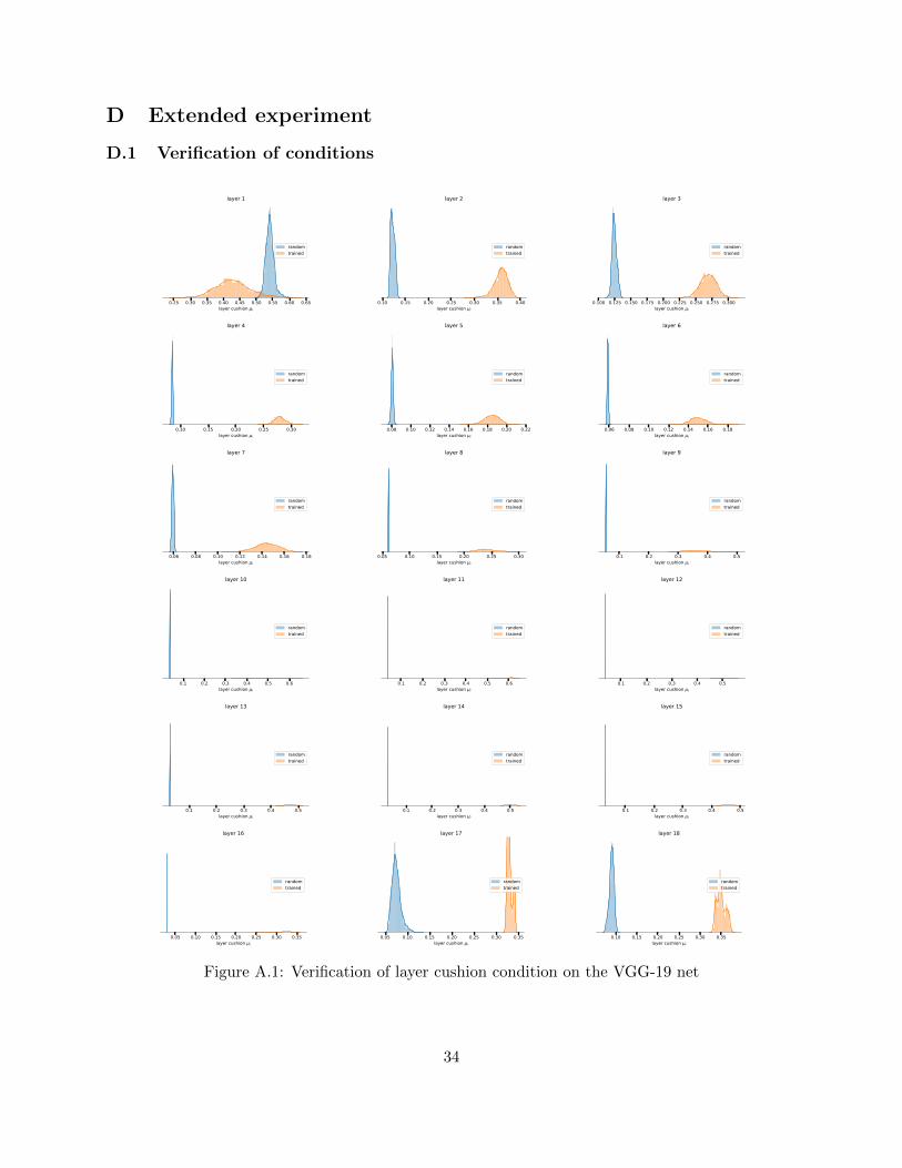
D Extended experiment

D.1 Verification of conditions

0.25 0.30 0.35 0.40 0.45 0.50 0.55 0.60 0.65layer cushion i

layer 1

randomtrained

0.10 0.15 0.20 0.25 0.30 0.35 0.40layer cushion i

layer 2

randomtrained

0.100 0.125 0.150 0.175 0.200 0.225 0.250 0.275 0.300layer cushion i

layer 3

randomtrained

0.10 0.15 0.20 0.25 0.30layer cushion i

layer 4

randomtrained

0.08 0.10 0.12 0.14 0.16 0.18 0.20 0.22layer cushion i

layer 5

randomtrained

0.06 0.08 0.10 0.12 0.14 0.16 0.18layer cushion i

layer 6

randomtrained

0.06 0.08 0.10 0.12 0.14 0.16 0.18layer cushion i

layer 7

randomtrained

0.05 0.10 0.15 0.20 0.25 0.30layer cushion i

layer 8

randomtrained

0.1 0.2 0.3 0.4 0.5layer cushion i

layer 9

randomtrained

0.1 0.2 0.3 0.4 0.5 0.6layer cushion i

layer 10

randomtrained

0.1 0.2 0.3 0.4 0.5 0.6layer cushion i

layer 11

randomtrained

0.1 0.2 0.3 0.4 0.5layer cushion i

layer 12

randomtrained

0.1 0.2 0.3 0.4 0.5layer cushion i

layer 13

randomtrained

0.1 0.2 0.3 0.4 0.5layer cushion i

layer 14

randomtrained

0.1 0.2 0.3 0.4 0.5layer cushion i

layer 15

randomtrained

0.05 0.10 0.15 0.20 0.25 0.30 0.35layer cushion i

layer 16

randomtrained

0.05 0.10 0.15 0.20 0.25 0.30 0.35layer cushion i

layer 17

randomtrained

0.10 0.15 0.20 0.25 0.30 0.35layer cushion i

layer 18

randomtrained

Figure A.1: Verification of layer cushion condition on the VGG-19 net

34

0.05 0.10 0.15 0.20 0.25 0.30 0.35 0.40interlayer cushion i, j

layer 1 -> layer 19

randomtrained

0.1 0.2 0.3 0.4 0.5 0.6 0.7interlayer cushion i, j

layer 2 -> layer 19

randomtrained

0.0 0.2 0.4 0.6 0.8 1.0interlayer cushion i, j

layer 3 -> layer 19

randomtrained

0.2 0.4 0.6 0.8 1.0interlayer cushion i, j

layer 4 -> layer 19

randomtrained

0.1 0.2 0.3 0.4 0.5 0.6 0.7 0.8interlayer cushion i, j

layer 5 -> layer 19

randomtrained

0.1 0.2 0.3 0.4 0.5 0.6 0.7 0.8 0.9interlayer cushion i, j

layer 6 -> layer 19

randomtrained

0.0 0.2 0.4 0.6 0.8interlayer cushion i, j

layer 7 -> layer 19

randomtrained

0.2 0.4 0.6 0.8interlayer cushion i, j

layer 8 -> layer 19

randomtrained

0.2 0.4 0.6 0.8 1.0interlayer cushion i, j

layer 9 -> layer 19

randomtrained

0.2 0.3 0.4 0.5 0.6 0.7 0.8 0.9interlayer cushion i, j

layer 10 -> layer 19

randomtrained

0.1 0.2 0.3 0.4 0.5interlayer cushion i, j

layer 11 -> layer 19

randomtrained

0.1 0.2 0.3 0.4 0.5interlayer cushion i, j

layer 12 -> layer 19

randomtrained

0.2 0.4 0.6 0.8 1.0interlayer cushion i, j

layer 13 -> layer 19

randomtrained

0.1 0.2 0.3 0.4 0.5interlayer cushion i, j

layer 14 -> layer 19

randomtrained

0.10 0.15 0.20 0.25 0.30 0.35 0.40 0.45interlayer cushion i, j

layer 15 -> layer 19

randomtrained

0.10 0.15 0.20 0.25 0.30 0.35 0.40 0.45 0.50interlayer cushion i, j

layer 16 -> layer 19

randomtrained

0.3 0.4 0.5 0.6 0.7 0.8 0.9 1.0interlayer cushion i, j

layer 17 -> layer 19

randomtrained

0.18 0.20 0.22 0.24 0.26 0.28 0.30 0.32 0.34interlayer cushion i, j

layer 18 -> layer 19

randomtrained

Figure A.2: Verification of interlayer cushion condition on the VGG-19 net

35

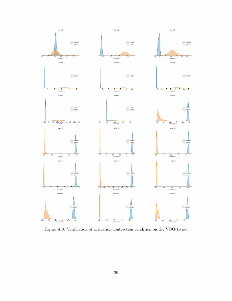
1.2 1.3 1.4 1.5 1.6 1.7contraction c

layer 1

randomtrained

1.4 1.6 1.8 2.0contraction c

layer 2

randomtrained

1.2 1.4 1.6 1.8 2.0 2.2 2.4contraction c

layer 3

randomtrained

2 3 4 5 6contraction c

layer 4

randomtrained

1.5 2.0 2.5 3.0 3.5 4.0contraction c

layer 5

randomtrained

1.5 2.0 2.5 3.0 3.5 4.0 4.5 5.0contraction c

layer 6

randomtrained

1.25 1.50 1.75 2.00 2.25 2.50 2.75 3.00 3.25contraction c

layer 7

randomtrained

1.0 1.5 2.0 2.5 3.0contraction c

layer 8

randomtrained

1.0 1.1 1.2 1.3 1.4 1.5contraction c

layer 9

randomtrained

1.0 1.1 1.2 1.3 1.4contraction c

layer 10

randomtrained

1.0 1.1 1.2 1.3 1.4 1.5contraction c

layer 11

randomtrained

1.0 1.1 1.2 1.3 1.4contraction c

layer 12

randomtrained

1.0 1.1 1.2 1.3 1.4 1.5contraction c

layer 13

randomtrained

1.00 1.05 1.10 1.15 1.20 1.25 1.30 1.35contraction c

layer 14

randomtrained

1.0 1.1 1.2 1.3 1.4contraction c

layer 15

randomtrained

1.15 1.20 1.25 1.30 1.35 1.40contraction c

layer 16

randomtrained

1.0 1.1 1.2 1.3 1.4contraction c

layer 17

randomtrained

1.0 1.1 1.2 1.3 1.4contraction c

layer 18

randomtrained

Figure A.3: Verification of activation contraction condition on the VGG-19 net

36

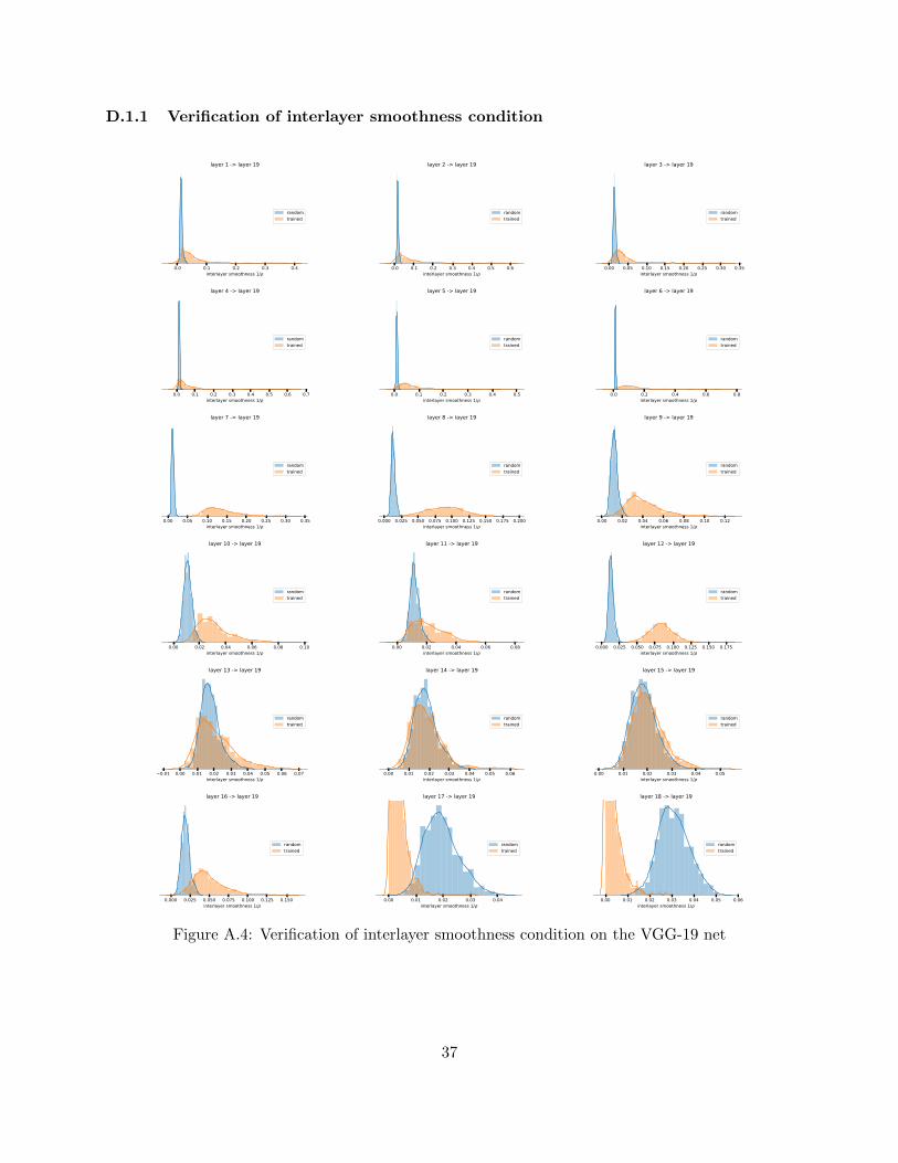
D.1.1 Verification of interlayer smoothness condition

0.0 0.1 0.2 0.3 0.4interlayer smoothness 1/

layer 1 -> layer 19

randomtrained

0.0 0.1 0.2 0.3 0.4 0.5 0.6interlayer smoothness 1/

layer 2 -> layer 19

randomtrained

0.00 0.05 0.10 0.15 0.20 0.25 0.30 0.35interlayer smoothness 1/

layer 3 -> layer 19

randomtrained

0.0 0.1 0.2 0.3 0.4 0.5 0.6 0.7interlayer smoothness 1/

layer 4 -> layer 19

randomtrained

0.0 0.1 0.2 0.3 0.4 0.5interlayer smoothness 1/

layer 5 -> layer 19

randomtrained

0.0 0.2 0.4 0.6 0.8interlayer smoothness 1/

layer 6 -> layer 19

randomtrained

0.00 0.05 0.10 0.15 0.20 0.25 0.30 0.35interlayer smoothness 1/

layer 7 -> layer 19

randomtrained

0.000 0.025 0.050 0.075 0.100 0.125 0.150 0.175 0.200interlayer smoothness 1/

layer 8 -> layer 19

randomtrained

0.00 0.02 0.04 0.06 0.08 0.10 0.12interlayer smoothness 1/

layer 9 -> layer 19

randomtrained

0.00 0.02 0.04 0.06 0.08 0.10interlayer smoothness 1/

layer 10 -> layer 19

randomtrained

0.00 0.02 0.04 0.06 0.08interlayer smoothness 1/

layer 11 -> layer 19

randomtrained

0.000 0.025 0.050 0.075 0.100 0.125 0.150 0.175interlayer smoothness 1/

layer 12 -> layer 19

randomtrained

0.01 0.00 0.01 0.02 0.03 0.04 0.05 0.06 0.07interlayer smoothness 1/

layer 13 -> layer 19

randomtrained

0.00 0.01 0.02 0.03 0.04 0.05 0.06interlayer smoothness 1/

layer 14 -> layer 19

randomtrained

0.00 0.01 0.02 0.03 0.04 0.05interlayer smoothness 1/

layer 15 -> layer 19

randomtrained

0.000 0.025 0.050 0.075 0.100 0.125 0.150interlayer smoothness 1/

layer 16 -> layer 19

randomtrained

0.00 0.01 0.02 0.03 0.04interlayer smoothness 1/

layer 17 -> layer 19

randomtrained

0.00 0.01 0.02 0.03 0.04 0.05 0.06interlayer smoothness 1/

layer 18 -> layer 19

randomtrained

Figure A.4: Verification of interlayer smoothness condition on the VGG-19 net

37

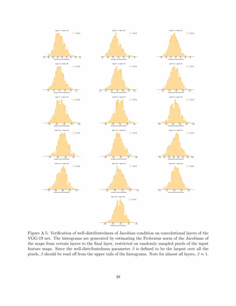
0.4 0.6 0.8 1.0 1.2 1.4 1.6 1.8 2.0average well-distributednes

layer 1 -> layer 19trained

0.6 0.8 1.0 1.2 1.4 1.6 1.8average well-distributednes

layer 2 -> layer 19trained

0.9 1.0 1.1 1.2 1.3 1.4 1.5average well-distributednes

layer 3 -> layer 19trained

1.0 1.1 1.2 1.3 1.4 1.5average well-distributednes

layer 4 -> layer 19trained

1.10 1.15 1.20 1.25 1.30 1.35 1.40average well-distributednes

layer 5 -> layer 19trained

1.20 1.25 1.30 1.35 1.40average well-distributednes

layer 6 -> layer 19trained

1.25 1.30 1.35 1.40 1.45average well-distributednes

layer 7 -> layer 19trained

1.25 1.30 1.35 1.40 1.45average well-distributednes

layer 8 -> layer 19trained

1.32 1.34 1.36 1.38 1.40 1.42average well-distributednes

layer 9 -> layer 19trained

1.36 1.38 1.40 1.42average well-distributednes

layer 10 -> layer 19trained

1.28 1.30 1.32 1.34 1.36average well-distributednes

layer 11 -> layer 19trained

1.32 1.33 1.34 1.35 1.36 1.37 1.38 1.39average well-distributednes

layer 12 -> layer 19trained

1.07 1.08 1.09 1.10 1.11average well-distributednes

layer 13 -> layer 19trained

1.08 1.09 1.10 1.11 1.12average well-distributednes

layer 14 -> layer 19trained

1.11 1.12 1.13 1.14 1.15average well-distributednes

layer 15 -> layer 19trained

1.09 1.10 1.11 1.12 1.13average well-distributednes

layer 16 -> layer 19trained

Figure A.5: Verification of well-distributedness of Jacobian condition on convolutional layers of theVGG-19 net. The histograms are generated by estimating the Frobenius norm of the Jacobians ofthe maps from certain layers to the final layer, restricted on randomly sampled pixels of the inputfeature maps. Since the well-distributedness parameter β is defined to be the largest over all thepixels, β should be read off from the upper tails of the histograms. Note for almost all layers, β ≈ 1.

38

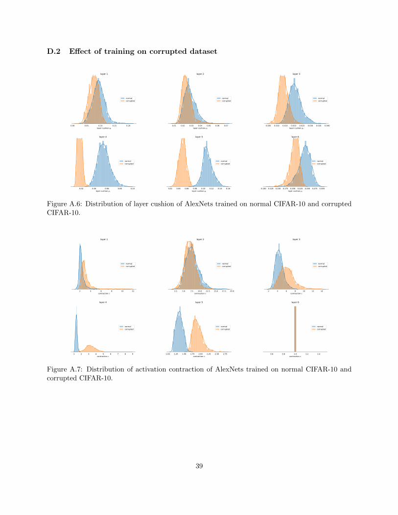
D.2 Effect of training on corrupted dataset

0.00 0.05 0.10 0.15 0.20layer cushion i

layer 1

normalcorrupted

0.01 0.02 0.03 0.04 0.05 0.06 0.07layer cushion i

layer 2

normalcorrupted

0.005 0.010 0.015 0.020 0.025 0.030 0.035 0.040layer cushion i

layer 3

normalcorrupted

0.02 0.04 0.06 0.08 0.10layer cushion i

layer 4

normalcorrupted

0.02 0.04 0.06 0.08 0.10 0.12 0.14 0.16layer cushion i

layer 5

normalcorrupted

0.100 0.125 0.150 0.175 0.200 0.225 0.250 0.275 0.300layer cushion i

layer 6

normalcorrupted

Figure A.6: Distribution of layer cushion of AlexNets trained on normal CIFAR-10 and corruptedCIFAR-10.

2 4 6 8 10 12contraction c

layer 1

normalcorrupted

2.5 5.0 7.5 10.0 12.5 15.0 17.5 20.0contraction c

layer 2

normalcorrupted

2 4 6 8 10 12 14contraction c

layer 3

normalcorrupted

1 2 3 4 5 6 7 8 9contraction c

layer 4

normalcorrupted

1.00 1.25 1.50 1.75 2.00 2.25 2.50 2.75contraction c

layer 5

normalcorrupted

0.6 0.8 1.0 1.2 1.4contraction c

layer 6

normalcorrupted

Figure A.7: Distribution of activation contraction of AlexNets trained on normal CIFAR-10 andcorrupted CIFAR-10.

39