, , 1{29 ()c Kluwer Academic Publishers, Boston. Manufactured in The Netherlands.Cascade GeneralizationJO~AO GAMA jgama@ncc.up.ptPAVEL BRAZDIL pbrazdil@ncc.up.ptLIACC, FEP - University of PortoRua Campo Alegre, 8234150 Porto, PortugalPhone: (+351) 2 6078830 Fax: (+351) 2 6003654http://www.ncc.up.pt/liacc/MLEditor:Abstract. Using multiple classi�ers for increasing learning accuracy is an active researcharea. In this paper we present two related methods for merging classi�ers. The �rst method,Cascade Generalization, couples classi�ers loosely. It belongs to the family of stacking algorithms.The basic idea of Cascade Generalization is to use sequentially the set of classi�ers, at each stepperforming an extension of the original data by the insertion of new attributes. The new attributesare derived from the probability class distribution given by a base classi�er. This constructive stepextends the representational language for the high level classi�ers, relaxing their bias. The secondmethod exploits tight coupling of classi�ers, by applying Cascade Generalization locally. At eachiteration of a divide and conquer algorithm, a reconstruction of the instance space occurs by theaddition of new attributes. Each new attribute represents the probability that an example belongsto a class given by a base classi�er. We have implemented three Local Generalization Algorithms.The �rst merges a linear discriminant with a decision tree, the second merges a naive Bayes witha decision tree, and the third merges a linear discriminant and a naive Bayes with a decisiontree. All the algorithms show an increase of performance, when compared with the correspondingsingle models. Cascade also outperforms other methods for combining classi�ers, like StackedGeneralization, and competes well against Boosting at statistically signi�cant con�dence levels.Keywords: Multiple Models, Constructive Induction, Merging Classi�ers.1. IntroductionThe ability of a chosen classi�cation algorithm to induce a good generalization de-pends on the appropriateness of its representation language to express generaliza-tions of the examples for the given task. The representation language for a standarddecision tree is the DNF formalism that splits the instance space by axis-parallelhyper-planes, while the representation language for a linear discriminant function isa set of linear functions that split the instance space by oblique hyper planes. Sincedi�erent learning algorithms employ di�erent knowledge representations and searchheuristics, di�erent search spaces are explored and diverse results are obtained. Instatistics, Henery (1997) refers to rescaling as a method used when some classesare over-predicted leading to a bias. Rescaling consists of applying the algorithmsin sequence, the output of an algorithm being used as input to another algorithm.The aim would be to use the estimated probabilities Wi = P (CijX) derived from alearning algorithm, as input to a second learning algorithm the purpose of which is

2to produce an unbiased estimate Q(CijW ) of the conditional probability for classCi.The problem of �nding the appropriate bias for a given task is an active researcharea. We can consider two main lines: on the one hand, methods that try to selectthe most appropriate algorithm for the given task, for instance Scha�er's selectionby Cross-Validation, and on the other hand, methods that combine predictions ofdi�erent algorithms, for instance Stacked Generalization (Wolpert 1992). The workpresented here near follows the second research line. Instead of looking for methodsthat �t the data using a single representation language, we present a family ofalgorithms, under the generic name of Cascade Generalization, whose search spacecontains models that use di�erent representation languages. Cascade generalizationperforms an iterative composition of classi�ers. At each iteration a classi�er isgenerated. The input space is extended by the addition of new attributes. These arein the form of a probability class distribution which are obtained, for each example,by the generated classi�er. The language of the �nal classi�er is the language usedby the high level generalizer. This language uses terms that are expressions fromthe language of low level classi�ers. In this sense, Cascade Generalization generatesa uni�ed theory from the base theories.Here we extend the work presented in (Gama 1998) by applying Cascade locally.In our implementation, Local Cascade Generalization generates a decision tree. Theexperimental study shows that this methodology usually improves both accuracyand theory size at statistically signi�cant levels.In the next Section we review previous work in the area of multiple models.In Section 3 we present the framework of Cascade Generalization. In Section 4we discuss the strengths and weaknesses of the proposed method in comparisonto other approaches to multiple models. In Section 5 we perform an empiricalevaluation of Cascade Generalization using UCI data sets. In Section 6 we de�ne anew family of multi-strategy algorithms that apply Cascade Generalization locally.In Section 7, we empirically evaluate Local Cascade Generalization using UCI datasets. In Section 8, we examine the behavior of Cascade Generalization providinginsights about why it works. The last Section summarizes the main points of thework, and discusses future research directions.2. Related Work on Combining Classi�ersVoting is the most common method used to combine classi�ers. As pointed out byAli and Pazzani (1996), this strategy is motivated by the Bayesian learning theorywhich stipulates that in order to maximize the predictive accuracy, instead of usingjust a single learning model, one should ideally use all models in the hypothesisspace. The vote of each hypothesis should be weighted by the posterior probabilityof that hypothesis given the training data. Several variants of the voting methodcan be found in the machine learning literature. From uniform voting where theopinion of all base classi�ers contributes to the �nal classi�cation with the samestrength, to weighted voting, where each base classi�er has a weight associated,

3that could change over the time, and strengthens the classi�cation given by theclassi�er.Another approach to combine classi�ers consists of generating multiple models.Several methods appear in the literature. In this paper we analyze them throughBias-Variance analysis (Kohavi & Wolpert, 1996): methods that mainly reducevariance, like Bagging and Boosting, and methods that mainly reduce bias, likeStacked Generalization and Meta-Learning.2.1. Variance Reduction MethodsBreiman (1996) proposes Bagging, that produces replications of the training setby sampling with replacement. Each replication of the training set has the samesize as the original data but some examples do not appear in it while others mayappear more than once. From each replication of the training set a classi�er isgenerated. All classi�ers are used to classify each example in the test set, usuallyusing a uniform vote scheme.The Boosting algorithm of Freund and Schapire (1996) maintains a weight foreach example in the training set that re ects its importance. Adjusting the weightscauses the learner to focus on di�erent examples leading to di�erent classi�ers.Boosting is an iterative algorithm. At each iteration the weights are adjusted inorder to re ect the performance of the corresponding classi�er. The weight ofthe misclassi�ed examples is increased. The �nal classi�er aggregates the learnedclassi�ers at each iteration by weighted voting. The weight of each classi�er is afunction of its accuracy.2.2. Bias Reduction MethodsWolpert (1992) proposed Stacked Generalization, a technique that uses learning intwo levels. A learning algorithm is used to determine how the outputs of the baseclassi�ers should be combined. The original data set constitutes the level zero data.All the base classi�ers run at this level. The level one data are the outputs of thebase classi�ers. Another learning process occurs using as input the level one dataand as output the �nal classi�cation. This is a more sophisticated technique ofcross validation that could reduce the error due to the bias.Chan and Stolfo (1995) present two schemes for classi�er combination: arbiterand combiner. Both schemes are based on meta learning, where a meta-classi�eris generated from meta data, built based on the predictions of the base classi�ers.An arbiter is also a classi�er and is used to arbitrate among predictions generatedby di�erent base classi�ers. The training set for the arbiter is selected from all theavailable data, using a selection rule. An example of a selection rule is \Select theexamples whose classi�cation the base classi�ers cannot predict consistently". Thisarbiter, together with an arbitration rule, decides a �nal classi�cation based on thebase predictions. An example of an arbitration rule is \Use the prediction of thearbiter when the base classi�ers cannot obtain a majority". Later (Chan & Stolfo

41995a), this framework was extended using arbiters/combiners in an hierarchicalfashion, generating arbiter/combiner binary trees.Skalak (1997) presents an excellent dissertation discussing methods for combiningclassi�ers. He presents several algorithms most of which are based on StackedGeneralization able to improve the performance of Nearest Neighbor classi�ers.Brodley (1995) presents MCS, a hybrid algorithm that combines, in a single tree,nodes that are univariate tests, multivariate tests generated by linear machines andinstance based learners. At each node MCS uses a set of If-Then rules to performa hill-climbing search for the best hypothesis space and search bias for the givenpartition of the dataset. The set of rules incorporates knowledge of experts. MCSuses a dynamic search control strategy to perform an automatic model selection.MCS builds trees which can apply a di�erent model in di�erent regions of theinstance space.2.3. DiscussionEarlier results of Boosting or Bagging are quite impressive. Using 10 iterations(i.e. generating 10 classi�ers) Quinlan (1996) reports reductions of the error ratebetween 10% and 19%. Quinlan argues that these techniques are mainly applicablefor unstable classi�ers. Both techniques require that the learning system not bestable, to obtain di�erent classi�ers when there are small changes in the trainingset. Under an analysis of bias-variance decomposition of the error (Kohavi 1996),the reduction of the error observed with Boosting or Bagging is mainly due to thereduction in the variance. Breiman (1996) reveals that Boosting and Bagging canonly improve the predictive accuracy of learning algorithms that are \unstable".As mentioned in Kohavi and Bauer (1998) the main problem with Boosting seemsto be robustness to noise. This is expected because noisy examples tend to be mis-classi�ed, and the weight will increase for these examples. They present severalcases were the performance of Boosting algorithms degraded compared to the orig-inal algorithms. They also point out that Bagging improves in all datasets used inthe experimental evaluation. They conclude that although Boosting is on averagebetter than Bagging, it is not uniformly better than Bagging. The higher accuracyof Boosting over Bagging in many domains was due to a reduction of bias. Boostingwas also found to frequently have higher variance than Bagging.Boosting and Bagging require a considerable number of member models becausethey rely on varying the data distribution to get a diverse set of models from asingle learning algorithm.Wolpert (1992) says that successful implementation of Stacked Generalization forclassi�cation tasks is a \black art", and the conditions under which stacking worksare still unknown:For example, there are currently no hard and fast rules saying what level0generalizers should we use, what level1 generalizer one should use, what knumbers to use to form the level1 input space, etc.

5Recently, Ting and Witten (1997) have shown that successful stacked generaliza-tion requires the use of output class distributions rather than class predictions. Intheir experiments only the MLR algorithm (a linear discriminant) was suitable forlevel-1 generalizer.3. Cascade GeneralizationConsider a learning set D = ( ~xn; yn) with n = 1; :::; N , where ~xi = [x1; :::; xm] isa multidimensional input vector, and yn is the output variable. Since the focus ofthis paper is on classi�cation problems, yn takes values from a set of prede�nedvalues, that is yn 2 fCl1; :::; Clcg, where c is the number of classes. A classi�er= is a function that is applied to the training set D to construct a model =(D).The generated model is a mapping from the input space X to the discrete outputvariable Y . When used as a predictor, represented by =(~x;D), it assigns a yvalue to the example ~x. This is the traditional framework for classi�cation tasks.Our framework requires that the predictor =(~x;D) outputs a vector representingconditional probability distribution [p1; :::; pc], where pi represents the probabilitythat the example ~x belongs to class i, i.e. P (y = Clij~x). The class that is assignedto the example ~x, is the one that maximizes this last expression. Most of thecommonly used classi�ers, such as naive Bayes and Discriminant, classify eachexample in this way. Other classi�ers, for example C4.5, have a di�erent strategyfor classifying an example, but it requires few changes to obtain a probability classdistribution.We de�ne a constructive operator '(~x;M) where M represents the model =(D)for the training data D, while ~x represents an example. For the example ~x theoperator ' concatenates the input vector ~x with the output probability class dis-tribution. If the operator ' is applied to all examples of dataset D0 we obtain anew dataset D00. The cardinality of D00 is equal to the cardinality of D0 (i.e. theyhave the same number of examples). Each example in ~x 2 D00 has an equivalentexample in D0, but augmented with #c new attributes, where #c represents thenumber of classes. The new attributes are the elements of the vector of class prob-ability distribution obtained when applying classi�er =(D) to the example ~x. Thiscan be represented formally as follows:D00 = �(D0;A(=(D);D0)) (1)Here A(=(D);D0) represents the application of the model =(D) to data set D0 andrepresents, in e�ect, a dataset. This dataset contains all the examples that appearinD0 extended with the probability class distribution generated by the model =(D).Cascade generalization is a sequential composition of classi�ers, that at eachgeneralization level applies the � operator. Given a training set L, a test set T,and two classi�ers =1, and =2, Cascade generalization proceeds as follows: Usingclassi�er =1, generates the Level1 data:Level1train = �(L;A(=(L); L)) (2)

6 Level1test = �(T;A(=(L); T )) (3)Classi�er =2 learns on Level1 training data and classi�es the Level1 test data:A(=2(Level1train); Level1test)These steps perform the basic sequence of a cascade generalization of classi�er =2after classi�er =1. We represent the basic sequence by the symbol r. The previouscomposition could be represented succinctly by:=2r=1 = A(=2(Level1Train); Level1Test)which, by applying equations 2 and 3, is equivalent to:=2r=1 = A(=2(�(L;A(=1(L); L)));�(T;A(=1(L); T )))This is the simplest formulation of Cascade Generalization. Some possible ex-tensions include the composition of n classi�ers, and the parallel composition ofclassi�ers.A composition of n classi�ers is represented by:=nr=n�1r=n�2:::r=1In this case, Cascade Generalization generates n-1 levels of data. The �nal modelis the one given by the =n classi�er. This model could contain terms in the formof conditions based on attributes build by the previous built classi�ers.A variant of cascade generalization, which includes several algorithms in parallel,could be represented in this formalism by:=nr[=1; :::;=n�1] =A(=n(�p(L; [A(=1(L); L); :::;A(=n�1(L); L)])); (�p(T; [A(=1(L); T ); :::;A(=n�1(L); T )])))The algorithms =1, ..., =n�1 run in parallel. The operator�p(L; [A(=1(L); L); :::;A(=n�1(L); L)])returns a new data set L0 which contains the same number of examples as L. Eachexample in L0 contains (n � 1) �#cl new attributes, where #cl is the number ofclasses. Each algorithm in the set =1; :::;=n�1 contributes with #cl new attributes.3.1. An Illustrative ExampleIn this example we will consider the UCI data set Monks-2 (Thrun et al. 1991).The Monks data sets describe an arti�cial robot domain and are quite well knownin the Machine Learning community. The robots are described by six di�erentattributes and classi�ed into one of two classes. We have chosen the Monks-2problem because it is known that this is a di�cult task for systems that learndecision trees in attribute-value formalism. The decision rule for the problem is:\The robot is O.K. if exactly two of the six attributes have their �rstvalue". This problem is similar to parity problems. It combines di�erent attributesin a way that makes it complicated to describe in DNF or CNF using the givenattributes only.Some examples of the original training data are presented:

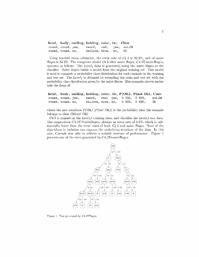
7head, body, smiling, holding, color, tie, Classround, round, yes, sword, red, yes, not Okround, round, no, balloon, blue, no, OKUsing ten-fold cross validation, the error rate of C4.5 is 32.9%, and of naiveBayes is 34.2%. The composite model C4.5 after naive Bayes, C4:5rnaiveBayes,operates as follows. The Level1 data is generated, using the naive Bayes as theclassi�er. Naive Bayes builds a model from the original training set. This modelis used to compute a probability class distribution for each example in the trainingand test set. The Level1 is obtained by extending the train and test set with theprobability class distribution given by the naive Bayes. The examples shown earliertake the form of:head, body, smiling, holding, color, tie, P(OK), P(not Ok), Classround, round, yes, sword, red, yes, 0.135, 0.864, not Okround, round, no, balloon, blue, no, 0.303, 0.696, OKwhere the new attribute P(OK) (P(not OK)) is the probability that the examplebelongs to class OK(not OK).C4.5 is trained on the Level 1 training data, and classi�es the Level 1 test data.The composition C4:5rNaiveBayes, obtains an error rate of 8.9%, which is sub-stantially lower than the error rates of both C4.5 and naive Bayes. None of thealgorithms in isolation can capture the underlying structure of the data. In thiscase, Cascade was able to achieve a notable increase of performance. Figure 1presents one of the trees generated by C4:5rnaiveBayes.P(OK)

tie ?

> 0.27

smiling ?

<= 0.27

P(OK)

Yes

smiling ?

No

not OK

Yes

tie ?

No

smiling ?

> 0.32

not OK

<= 0.32

P(not Ok)

Yes

P(not Ok)

No

P(not Ok)

Yes

not OK

No

P(not Ok)

Yes

P(not Ok)

No

OK

> 0.69

not OK

<= 0.69

OK

> 0.68

not OK

<= 0.68

not OK

> 0.8

OK

<= 0.8

not OK

> 0.62

OK

<= 0.62

OK

> 0.6

not OK

<= 0.6Figure 1. Tree generated by C4.5rBayes

8 The tree contains a mixture of some of the original attributes (smiling, tie) withsome of the new attributes constructed by naive Bayes (P(OK), P(not Ok)). Atthe root of the tree appears the attribute P(OK). This attribute represents a par-ticular class probability (Class = OK) calculated by naive Bayes. The decisiontree generated by C4.5 uses the constructed attributes given by Naive Bayes, butrede�ning di�erent thresholds. Because this is a two class problem, the Bayes ruleuses P (OK) with threshold 0.5, while the decision tree sets the threshold to 0.27.Those decision nodes are a kind of function given by the Bayes strategy. For exam-ple, the attribute P(OK) can be seen as a function that computes p(Class = OKj~x)using the Bayes theorem. On some branches the decision tree performs more thanone tests of the class probabilities. In a certain sense, this decision tree combinestwo representation languages: that of naive Bayes with the language of decisiontrees. The constructive step performed by Cascade, inserts new attributes thatincorporate new knowledge provided by the naive Bayes. It is this new knowledgethat allows the signi�cant increase of performance veri�ed with the decision tree,despite the fact that naive Bayes cannot �t well complex spaces. In the Cascadeframework lower level learners delay the decisions to the high level learners. It isthis kind of collaboration between classi�ers that Cascade Generalization explores.4. DiscussionCascade Generalization belongs to the family of stacking algorithms. Wolpert(1992) de�nes Stacking Generalization as a general framework for combining clas-si�ers. It involves taking the predictions from several classi�ers and using thesepredictions as the basis for the next stage of classi�cation.Cascade Generalization may be regarded as a special case of Stacking Generaliza-tion mainly due to the layered learning structure. Some aspects that make CascadeGeneralization particular, are:� The new attributes are continuous. They take the form of a probability classdistribution. Combining classi�ers by means of categorical classes looses thestrength of the classi�er in its prediction. The use of probability class distribu-tions allows us to explore that information.� All classi�ers have access to the original attributes. Any new attribute builtat lower layers is considered exactly in the same way as any of the originalattributes.� Cascade Generalization does not use internal Cross Validation. This aspecta�ects the computational e�ciency of Cascade.Many of these ideas has been discussed in literature. Ting (1997) has used probabil-ity class distributions as level-1 attributes, but did not use the original attributes.The possibility of using the original attributes and class predictions as level1 at-tributes as been pointed out by Wolpert in the original paper of Stacked Gener-alization. Skalak (1997) refers that Scha�er has used the original attributes and

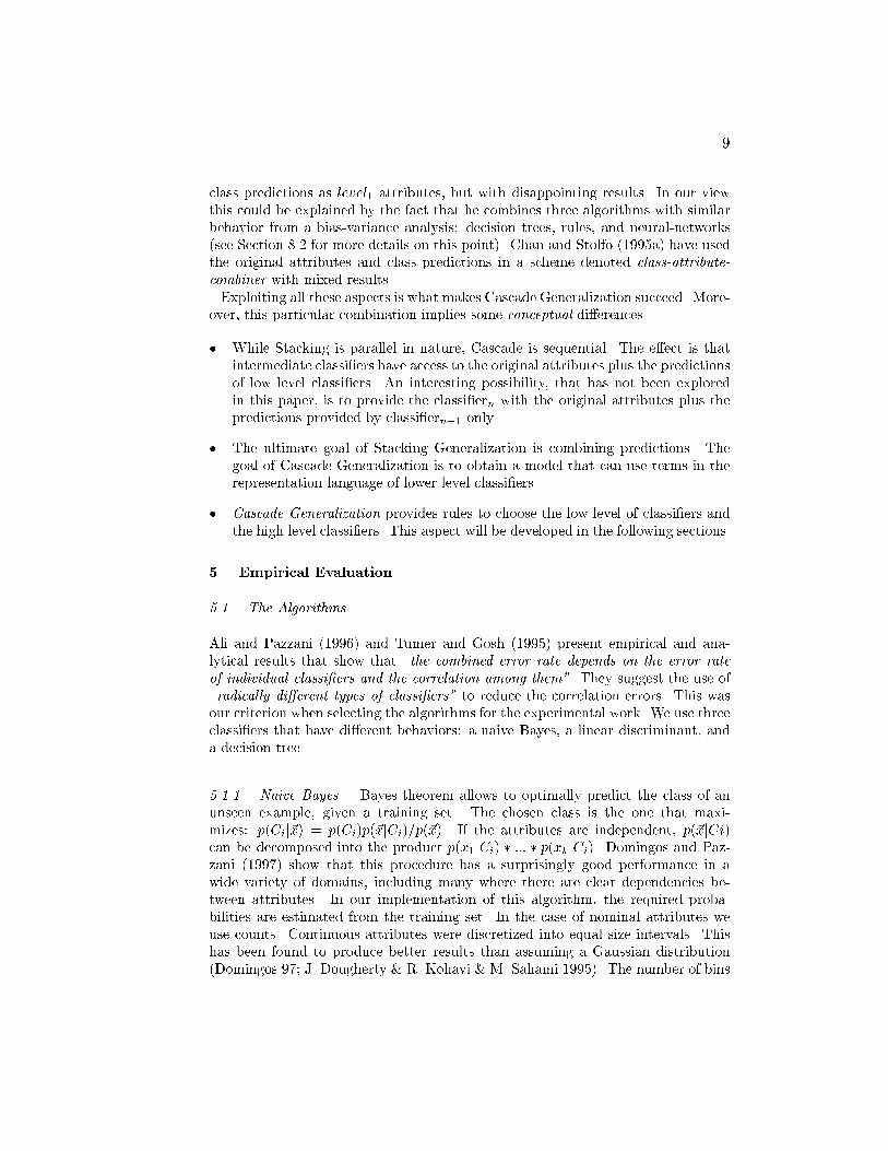
9class predictions as level1 attributes, but with disappointing results. In our viewthis could be explained by the fact that he combines three algorithms with similarbehavior from a bias-variance analysis: decision trees, rules, and neural-networks(see Section 8.2 for more details on this point). Chan and Stolfo (1995a) have usedthe original attributes and class predictions in a scheme denoted class-attribute-combiner with mixed results.Exploiting all these aspects is what makes Cascade Generalization succeed. More-over, this particular combination implies some conceptual di�erences.� While Stacking is parallel in nature, Cascade is sequential. The e�ect is thatintermediate classi�ers have access to the original attributes plus the predictionsof low level classi�ers. An interesting possibility, that has not been exploredin this paper, is to provide the classi�ern with the original attributes plus thepredictions provided by classi�ern�1 only.� The ultimate goal of Stacking Generalization is combining predictions. Thegoal of Cascade Generalization is to obtain a model that can use terms in therepresentation language of lower level classi�ers.� Cascade Generalization provides rules to choose the low level of classi�ers andthe high level classi�ers. This aspect will be developed in the following sections.5. Empirical Evaluation5.1. The AlgorithmsAli and Pazzani (1996) and Tumer and Gosh (1995) present empirical and ana-lytical results that show that \the combined error rate depends on the error rateof individual classi�ers and the correlation among them". They suggest the use of\radically di�erent types of classi�ers" to reduce the correlation errors. This wasour criterion when selecting the algorithms for the experimental work. We use threeclassi�ers that have di�erent behaviors: a naive Bayes, a linear discriminant, anda decision tree.5.1.1. Naive Bayes. Bayes theorem allows to optimally predict the class of anunseen example, given a training set. The chosen class is the one that maxi-mizes: p(Cij~x) = p(Ci)p(~xjCi)=p(~x). If the attributes are independent, p(~xjCi)can be decomposed into the product p(x1jCi) � ::: � p(xk jCi). Domingos and Paz-zani (1997) show that this procedure has a surprisingly good performance in awide variety of domains, including many where there are clear dependencies be-tween attributes. In our implementation of this algorithm, the required proba-bilities are estimated from the training set. In the case of nominal attributes weuse counts. Continuous attributes were discretized into equal size intervals. Thishas been found to produce better results than assuming a Gaussian distribution(Domingos 97; J. Dougherty & R. Kohavi & M. Sahami 1995). The number of bins

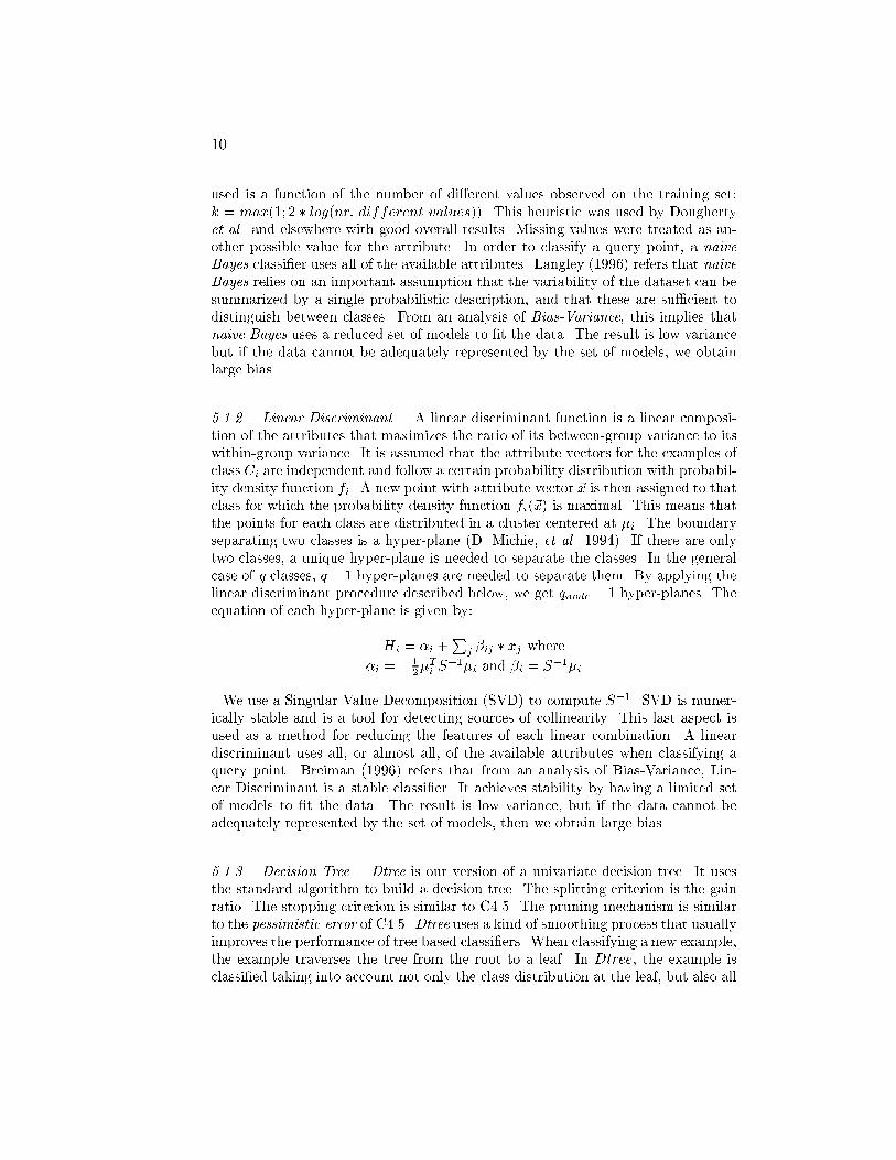
10used is a function of the number of di�erent values observed on the training set:k = max(1; 2 � log(nr: different values)). This heuristic was used by Doughertyet al. and elsewhere with good overall results. Missing values were treated as an-other possible value for the attribute. In order to classify a query point, a naiveBayes classi�er uses all of the available attributes. Langley (1996) refers that naiveBayes relies on an important assumption that the variability of the dataset can besummarized by a single probabilistic description, and that these are su�cient todistinguish between classes. From an analysis of Bias-Variance, this implies thatnaive Bayes uses a reduced set of models to �t the data. The result is low variancebut if the data cannot be adequately represented by the set of models, we obtainlarge bias.5.1.2. Linear Discriminant. A linear discriminant function is a linear composi-tion of the attributes that maximizes the ratio of its between-group variance to itswithin-group variance. It is assumed that the attribute vectors for the examples ofclass Ci are independent and follow a certain probability distribution with probabil-ity density function fi. A new point with attribute vector ~x is then assigned to thatclass for which the probability density function fi(~x) is maximal. This means thatthe points for each class are distributed in a cluster centered at �i. The boundaryseparating two classes is a hyper-plane (D. Michie, et al. 1994). If there are onlytwo classes, a unique hyper-plane is needed to separate the classes. In the generalcase of q classes, q � 1 hyper-planes are needed to separate them. By applying thelinear discriminant procedure described below, we get qnode � 1 hyper-planes. Theequation of each hyper-plane is given by:Hi = �i +Pj �ij � xj where�i = � 12�Ti S�1�i and �i = S�1�iWe use a Singular Value Decomposition (SVD) to compute S�1. SVD is numer-ically stable and is a tool for detecting sources of collinearity. This last aspect isused as a method for reducing the features of each linear combination. A lineardiscriminant uses all, or almost all, of the available attributes when classifying aquery point. Breiman (1996) refers that from an analysis of Bias-Variance, Lin-ear Discriminant is a stable classi�er. It achieves stability by having a limited setof models to �t the data. The result is low variance, but if the data cannot beadequately represented by the set of models, then we obtain large bias.5.1.3. Decision Tree. Dtree is our version of a univariate decision tree. It usesthe standard algorithm to build a decision tree. The splitting criterion is the gainratio. The stopping criterion is similar to C4.5. The pruning mechanism is similarto the pessimistic error of C4.5. Dtree uses a kind of smoothing process that usuallyimproves the performance of tree based classi�ers. When classifying a new example,the example traverses the tree from the root to a leaf. In Dtree, the example isclassi�ed taking into account not only the class distribution at the leaf, but also all

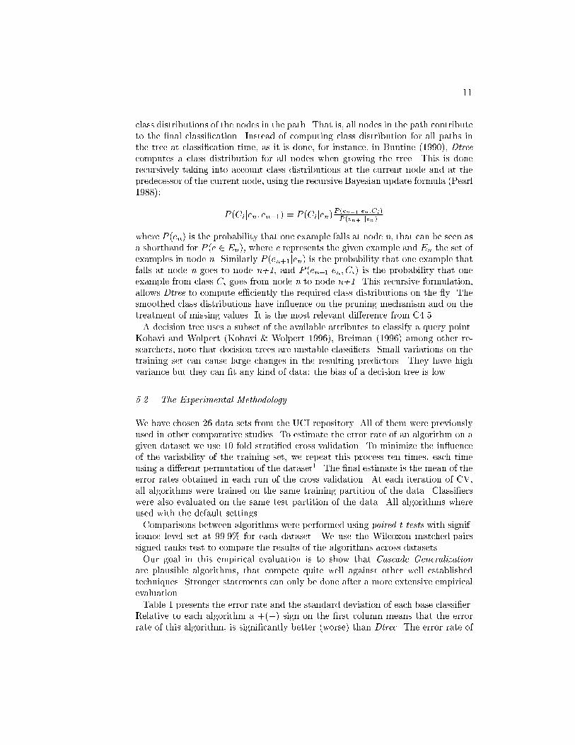
11class distributions of the nodes in the path. That is, all nodes in the path contributeto the �nal classi�cation. Instead of computing class distribution for all paths inthe tree at classi�cation time, as it is done, for instance, in Buntine (1990), Dtreecomputes a class distribution for all nodes when growing the tree. This is donerecursively taking into account class distributions at the current node and at thepredecessor of the current node, using the recursive Bayesian update formula (Pearl1988): P (Cijen; en+1) = P (Cijen)P (en+1jen;Ci)P (en+1jen)where P (en) is the probability that one example falls at node n, that can be seen asa shorthand for P (e 2 En), where e represents the given example and En the set ofexamples in node n. Similarly P (en+1jen) is the probability that one example thatfalls at node n goes to node n+1, and P (en+1jen; Ci) is the probability that oneexample from class Ci goes from node n to node n+1. This recursive formulation,allows Dtree to compute e�ciently the required class distributions on the y. Thesmoothed class distributions have in uence on the pruning mechanism and on thetreatment of missing values. It is the most relevant di�erence from C4.5.A decision tree uses a subset of the available attributes to classify a query point.Kohavi and Wolpert (Kohavi & Wolpert 1996), Breiman (1996) among other re-searchers, note that decision trees are unstable classi�ers. Small variations on thetraining set can cause large changes in the resulting predictors. They have highvariance but they can �t any kind of data: the bias of a decision tree is low.5.2. The Experimental MethodologyWe have chosen 26 data sets from the UCI repository. All of them were previouslyused in other comparative studies. To estimate the error rate of an algorithm on agiven dataset we use 10 fold strati�ed cross validation. To minimize the in uenceof the variability of the training set, we repeat this process ten times, each timeusing a di�erent permutation of the dataset1. The �nal estimate is the mean of theerror rates obtained in each run of the cross validation. At each iteration of CV,all algorithms were trained on the same training partition of the data. Classi�erswere also evaluated on the same test partition of the data. All algorithms whereused with the default settings.Comparisons between algorithms were performed using paired t-tests with signif-icance level set at 99.9% for each dataset. We use the Wilcoxon matched-pairssigned-ranks test to compare the results of the algorithms across datasets.Our goal in this empirical evaluation is to show that Cascade Generalizationare plausible algorithms, that compete quite well against other well establishedtechniques. Stronger statements can only be done after a more extensive empiricalevaluation.Table 1 presents the error rate and the standard deviation of each base classi�er.Relative to each algorithm a +(�) sign on the �rst column means that the errorrate of this algorithm, is signi�cantly better (worse) than Dtree. The error rate of

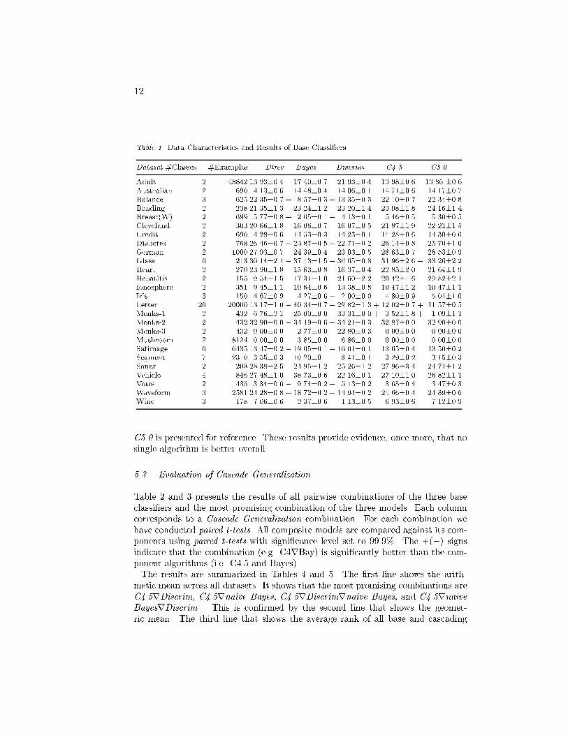
12Table 1. Data Characteristics and Results of Base Classi�ersDataset #Classes #Examples Dtree Bayes Discrim C4.5 C5.0Adult 2 48842 13.93�0.4 + 17.40�0.7 + 21.93�0.4 13.98�0.6 13.86 �0.6Australian 2 690 14.13�0.6 14.48�0.4 14.06�0.1 14.71�0.6 14.17�0.7Balance 3 625 22.35�0.7 + 8.57�0.3 + 13.35�0.3 22.10�0.7 22.34�0.8Banding 2 238 21.35�1.3 23.24�1.2 23.20�1.4 23.98�1.8 24.16�1.4Breast(W) 2 699 5.77�0.8 + 2.65�0.1 + 4.13�0.1 5.46�0.5 5.30�0.5Cleveland 2 303 20.66�1.8 + 16.06�0.7 + 16.07�0.5 21.87�1.9 22.21�1.5Credit 2 690 14.28�0.6 14.53�0.3 14.23�0.1 14.28�0.6 14.30�0.6Diabetes 2 768 26.46�0.7 + 23.87�0.5 + 22.71�0.2 26.14�0.8 25.70�1.0German 2 1000 27.93�0.7 + 24.39�0.4 + 23.03�0.5 28.63�0.7 28.53�0.9Glass 6 213 30.14�2.4 � 37.43�1.5 � 36.65�0.8 31.96�2.6 � 33.26�2.2Heart 2 270 23.90�1.8 + 15.63�0.8 + 16.37�0.4 22.85�2.0 21.64�1.9Hepatitis 2 155 19.54�1.5 17.31�1.0 21.60�2.2 20.42�1.6 20.82�2.1Ionosphere 2 351 9.45�1.1 10.64�0.6 � 13.38�0.8 10.47�1.2 10.47�1.1Iris 3 150 4.67�0.9 4.27�0.6 + 2.00�0.0 4.80�0.9 5.01�1.0Letter 26 20000 13.17�1.0 � 40.34�0.7 � 29.82�1.3 + 12.02�0.7 + 11.57�0.5Monks-1 2 432 6.76�2.1 � 25.00�0.0 � 33.31�0.0 + 3.52�1.8 + 1.09�1.1Monks-2 2 432 32.90�0.0 � 34.19�0.6 � 34.21�0.3 32.87�0.0 32.90�0.0Monks-3 2 432 0.00�0.0 � 2.77�0.0 � 22.80�0.3 0.00�0.0 0.00�0.0Mushroom 2 8124 0.00�0.0 � 3.85�0.0 � 6.86�0.0 0.00�0.0 0.00�0.0Satimage 6 6435 13.47�0.2 � 19.05�0.1 � 16.01�0.1 13.65�0.4 13.50�0.2Segment 7 2310 3.55�0.3 � 10.20�0.1 � 8.41�0.1 3.29�0.2 3.15�0.3Sonar 2 208 28.38�2.5 24.95�1.2 25.26�1.2 27.96�3.4 24.71�1.2Vehicle 4 846 27.48�1.0 � 38.73�0.6 + 22.16�0.1 27.10�1.0 26.82�1.1Votes 2 435 3.34�0.6 � 9.74�0.2 � 5.43�0.2 3.65�0.4 3.47�0.3Waveform 3 2581 24.28�0.8 + 18.72�0.2 + 14.94�0.2 24.66�0.4 24.89�0.6Wine 3 178 7.06�0.6 + 2.37�0.6 + 1.13�0.5 6.93�0.6 7.12�0.9C5.0 is presented for reference. These results provide evidence, once more, that nosingle algorithm is better overall.5.3. Evaluation of Cascade GeneralizationTable 2 and 3 presents the results of all pairwise combinations of the three baseclassi�ers and the most promising combination of the three models. Each columncorresponds to a Cascade Generalization combination. For each combination wehave conducted paired t-tests. All composite models are compared against its com-ponents using paired t-tests with signi�cance level set to 99.9%. The +(�) signsindicate that the combination (e.g. C4rBay) is signi�cantly better than the com-ponent algorithms (i.e. C4.5 and Bayes).The results are summarized in Tables 4 and 5. The �rst line shows the arith-metic mean across all datasets. It shows that the most promising combinations areC4.5rDiscrim, C4.5rnaive Bayes, C4.5rDiscrimrnaive Bayes, and C4.5rnaiveBayesrDiscrim . This is con�rmed by the second line that shows the geomet-ric mean. The third line that shows the average rank of all base and cascading

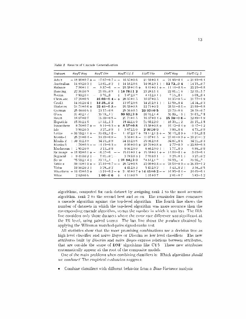
13Table 2. Results of Cascade GeneralizationDataset BayrBay BayrDis BayrC4.5 DisrDis DisrBay DisrC4.5Adult � 18.90�0.7 + + 17.07�0.7 + � 16.85�0.6 21.93�0.4 � 21.93�0.4 � 21.93�0.4Australian 14.69�0.5 + + 13.61�0.2 + 14.16�0.6 14.06�0.1 + + 12.72�0.4 + 14.15�0.7Balance 7.06�1.1 + 8.37�0.1 � � 23.38�1.0 + 8.41�0.1 + � 11.44�0.8 � 22.23�0.8Banding 22.36�0.9 21.99�0.8 + + 18.76�1.2 23.28�1.4 22.01�1.6 + 22.33�1.7Breast 2.83�0.1 � + 3.26�0.1 � + 3.42�0.2 4.13�0.1 + 2.75�0.1 � 5.08�0.4Cleveland 17.28�0.9 16.03�0.4� + 20.35�1.5 16.07�0.5 16.35�0.5 � 21.77�1.9Credit 14.91�0.4 + + 13.35�0.3 13.97�0.6 14.22�0.1 + + 13.59�0.4 14.34�0.3Diabetes 24.71�0.6 + 22.44�0.3� 25.33�0.8 22.71�0.2 23.51�0.6 � 25.99�0.8German � 25.48�0.6 + 23.17�0.6 � 28.56�0.5 23.03�0.5 23.73�0.6 � 28.58�0.7Glass 37.48�1.7 35.79�1.7 + 30.63�2.8 36.25�1.4 35.89�1.6 + 31.63�2.8Heart 16.67�0.7 16.30�0.5 � 21.74�1.5 16.37�0.4 + 15.56�0.6� 22.89�1.9Hepatitis 15.95�1.6 + 17.52�1.3 18.44�1.9 21.60�2.0 + 16.30�1.2 21.15�1.8Ionosphere 9.76�0.7 + + 9.14�0.3 + + 8.57�0.8 13.38�0.8 + 10.42�0.4 + 10.47�1.2Iris 3.80�0.5 � 3.27�0.9 + 3.67�1.0 2.00�0.0� + 3.00�0.4 � 4.73�0.9Letter + 36.59�1.1 + + 25.69�1.0 + 11.87�0.7 + 28.14�1.3 + � 36.42�0.9 + 11.94�0.8Monks-1 25.21�0.4 � 33.33�0.0 + 3.56�1.8 � 41.07�1.5 + 25.01�0.0 + � 20.21�4.2Monks-2 + 30.31�3.0 34.33�0.9 � 34.19�0.6 35.06�0.8 34.07�0.6 � 34.21�0.3Monks-3 1.76�0.8 � + 14.13�0.3 + 0.00�0.0 + 20.76�0.8 + 2.77�0.0 � 22.80�0.3Mushroom + 1.85�0.0 + 3.13�0.0 + 0.00�0.0 6.86�0.0 + + 1.77�0.0 � 6.86�0.0Satimage + 18.82�0.1 + � 16.57�0.1 + � 15.61�0.1 + 15.59�0.1 + + 14.84�0.1 + 13.63�0.4Segment + 9.41�0.2 + + 7.91�0.1 + � 3.78�0.3 + 7.93�0.1 � + 9.29�0.1 + 3.27�0.2Sonar 25.59�1.4 + + 23.72�1.1 + + 21.84�2.0 24.81�1.2 + 24.93�1.4 25.96�2.1Vehicle 39.16�1.0 + � 25.34�0.7 + � 28.52�0.8 22.00�0.3 � + 23.54�0.9 � + 26.33�1.2Votes 10.00�0.3 + 5.28�0.2 + � 4.41�0.3 5.43�0.2 + 5.43�0.2 + 3.56�0.5Waveform + 16.42�0.3 + 15.24�0.2 � + 21.80�0.7 + 14.45�0.2� + 16.93�0.4 � 24.65�0.4Wine 2.62�0.6 1.06�0.6� + 4.14�0.9 1.31�0.7 2.01�0.7 � 5.83�1.2algorithms, computed for each dataset by assigning rank 1 to the most accuratealgorithm, rank 2 to the second best and so on. The remainder lines comparesa cascade algorithm against the top-level algorithm. The fourth line shows thenumber of datasets in which the top-level algorithm was more accurate than thecorresponding cascade algorithm, versus the number in which it was less. The �fthline considers only those datasets where the error rate di�erence was signi�cant atthe 1% level, using paired t-tests. The last line shows the p-values obtained byapplying the Wilcoxon matched-pairs signed-ranks test.All statistics show that the most promising combinations use a decision tree ashigh-level classi�er and naive Bayes or Discrim as low-level classi�ers. The newattributes built by Discrim and naive Bayes express relations between attributes,that are outside the scope of DNF algorithms like C4.5. These new attributessystematically appear at the root of the composite models.One of the main problems when combining classi�ers is: Which algorithms shouldwe combine? The empirical evaluation suggests:� Combine classi�ers with di�erent behavior from a Bias-Variance analysis.

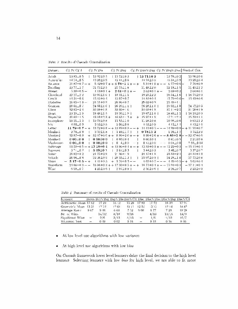
14Table 3. Results of Cascade GeneralizationDataset C4.5rC4.5 C4.5rDis C4.5rBay C4.5rDiscrBay C4.5rBayrDisc Stacked Gen.Adult + 13.85�0.5 + 13.92�0.5 + 13.72�0.3 + + 13.71�0.3 ++ 13.76�0.2 13.96�0.6Australian 14.74�0.5 13.99�0.9 15.41�0.8 14.24�0.5 15.34�0.9 13.99�0.4Balance 21.87�0.7 + + 5.42�0.7 + + 4.78�1.1+ ++ 5.34�1.0 + + + 6.77�0.6 � 7.76�0.9Banding 23.77�1.7 21.73�2.5 22.75�1.8 21.48�2.0 22.18�1.5 21.45�1.2Breast 5.36�0.5 + 4.13�0.1 + 2.61�0.1+ + 2.62�0.1 + + 2.69�0.2 2.66�0.1Cleveland 22.27�2.2 � 19.93�1.0 + 18.31�1.1 18.25�2.2 �� 20.54�1.6 + 16.75�0.9Credit 14.21�0.6 13.85�0.4 15.07�0.7 14.84�0.4 13.75�0.6 + 13.43�0.6Diabetes 26.05�1.0 +� 24.51�0.9 � 26.06�0.7 � 25.02�0.9 �� 25.48�1.4German 28.61�0.7 +� 24.60�1.0 +� 26.20�1.1 + �� 26.28�1.0 + � 25.92�1.0 + 24.72�0.3Glass 32.02�2.4 36.09�1.8 33.60�1.6 34.68�1.8 35.11�2.5 31.28�1.9Heart 23.19�1.9 + 18.48�1.5 � 19.30�1.9 + �� 18.67�1.0 + �� 18.89�1.1 + + 16.19�0.9Hepatitis 20.60�1.5 19.89�2.3 + 16.63�1.3 + + 15.97�1.9 17.21�2.1 15.33�1.1Ionosphere 10.21�1.3 + 10.79�0.8 11.55�1.0 + 11.28�0.8 + 10.98�0.6 9.63�1.2Iris 4.80�0.9 � 3.53�0.8 5.00�0.8 � 4.53�0.9 � 4.13�1.1 4.13�1.0Letter 11.79�0.7�+ 13.72�0.8 �+ 13.69�0.8 � ++ 14.41�0.5 � ++ 14.99�0.9 + + 11.91�0.7Monks-1 2.70�0.8 + 3.52�1.8 + 1.49�1.7 + + + 0.78�1.2 ++ 1.20�1.2 � 3.74�2.0Monks-2 32.87�0.0 + 32.87�0.0 + + 8.99�2.6 + + + 8.99�2.6 + + + 8.89�2.8� � 32.87�0.0Monks-3 0.00�0.0 + 0.00�0.0�+ 0.60�0.4 � ++ 0.60�0.4 � ++ 0.81�0.5 � � 2.24�0.8Mushroom 0.00�0.0 + 0.00�0.0�+ 0.14�0.0 � ++ 0.15�0.0 � ++ 0.04�0.0 � � 2.93�0.04Satimage 13.58�0.5 + + 12.18�0.4 + 13.06�0.4 + + + 12.83�0.3 + + + 12.22�0.3 � 13.11�0.4Segment 3.21�0.2 + 3.09�0.1 + 3.67�0.3 + + 3.44�0.3 + + 3.40�0.2 3.32�0.2Sonar 28.02�3.2 24.75�2.9 24.36�1.9 24.45�1.8 23.83�2.1 24.81�1.0Vehicle 26.96�0.8 + 22.36�0.9 + 28.35�1.3 + �+ 23.97�0.9 + +� 24.28�1.0 � � 27.72�0.8Votes + 3.17�0.5�+ 4.41�0.5 + 3.70�0.3 � + 4.62�0.7 � ++ 4.45�0.5 + + 3.65�0.4Waveform 24.66�0.3 +� 16.86�0.3 + + 17.30�0.5 + �+ 16.75�0.4 + �+ 15.94�0.3 � 17.14�0.4Wine 6.99�0.7 +� 4.25�0.6 + 2.97�0.9 + � 2.50�0.6 + � 2.26�0.7 2.23�0.9Table 4. Summary of results of Cascade GeneralizationMeasure Bayes BayrBay BayrDis BayrC4 Disc DiscrDisc DiscrBay DiscrC4Arithmetic Mean 17.62 17.29 16.42 15.29 17.80 17.72 16.39 17.94Geometric Mean 13.31 12.72 12.61 10.71 13.97 13.77 12.14 14.82Average Rank 9.67 9.46 6.63 7.52 9.06 8.77 7.23 10.29Nr. of Wins � 14/12 8/18 9/16 � 4/10 10/16 14/9Signi�cant Wins � 2/6 3/13 8/13 � 1/6 4/10 10/7Wilcoxon Test � 0.49 0.02 0.16 � 0.19 0.16 0.46� At low level use algorithms with low variance.� At high level use algorithms with low bias.On Cascade framework lower level learners delay the �nal decision to the high levellearners. Selecting learners with low bias for high level, we are able to �t more

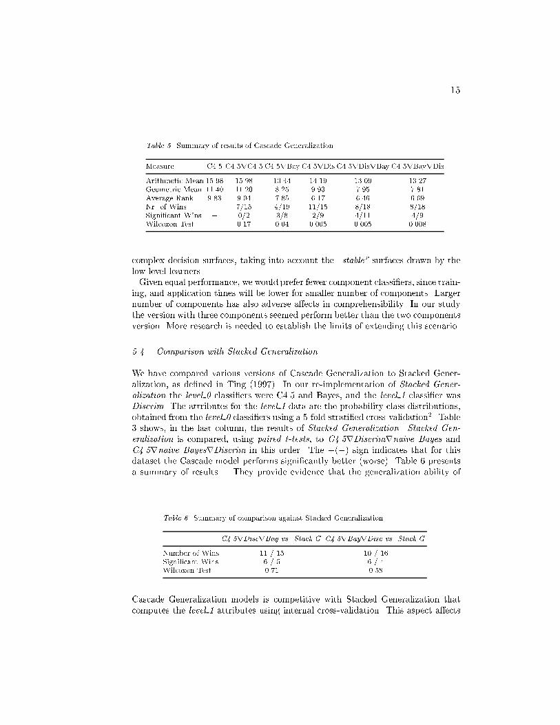
15Table 5. Summary of results of Cascade GeneralizationMeasure C4.5 C4.5rC4.5 C4.5rBay C4.5rDis C4.5rDisrBay C4.5rBayrDisArithmetic Mean 15.98 15.98 13.44 14.19 13.09 13.27Geometric Mean 11.40 11.20 8.25 9.93 7.95 7.81Average Rank 9.83 9.04 7.85 6.17 6.46 6.69Nr. of Wins � 7/15 4/19 11/15 8/18 8/18Signi�cant Wins � 0/2 3/8 2/9 4/11 4/9Wilcoxon Test � 0.17 0.04 0.005 0.005 0.008complex decision surfaces, taking into account the \stable" surfaces drawn by thelow level learners.Given equal performance, we would prefer fewer component classi�ers, since train-ing, and application times will be lower for smaller number of components. Largernumber of components has also adverse a�ects in comprehensibility. In our studythe version with three components seemed perform better than the two componentsversion. More research is needed to establish the limits of extending this scenario.5.4. Comparison with Stacked GeneralizationWe have compared various versions of Cascade Generalization to Stacked Gener-alization, as de�ned in Ting (1997). In our re-implementation of Stacked Gener-alization the level 0 classi�ers were C4.5 and Bayes, and the level 1 classi�er wasDiscrim. The attributes for the level 1 data are the probability class distributions,obtained from the level 0 classi�ers using a 5-fold strati�ed cross-validation2. Table3 shows, in the last column, the results of Stacked Generalization. Stacked Gen-eralization is compared, using paired t-tests, to C4.5rDiscrimrnaive Bayes andC4.5rnaive BayesrDiscrim in this order. The +(�) sign indicates that for thisdataset the Cascade model performs signi�cantly better (worse). Table 6 presentsa summary of results. They provide evidence that the generalization ability ofTable 6. Summary of comparison against Stacked GeneralizationC4.5rDiscrBay vs. Stack.G. C4.5rBayrDisc vs. Stack.G.Number of Wins 11 / 15 10 / 16Signi�cant Wins 6 / 5 6 / 4Wilcoxon Test 0.71 0.58Cascade Generalization models is competitive with Stacked Generalization thatcomputes the level 1 attributes using internal cross-validation. This aspect a�ects

16of course the learning times. Both Cascade models are at least three times fasterthan Stacked Generalization.Cascade Generalization exhibits good generalization ability and is computation-ally e�cient. Both aspects lead to the hypothesis: Can we improve Cascade Gen-eralization by applying it at each iteration of a divide-and-conquer algorithm? Thishypothesis is examined in the next section.6. Local Cascade GeneralizationMany classi�cation algorithms use a divide and conquer strategy that resolve agiven complex problem by dividing it into simpler problems, and then by applyingrecursively the same strategy to the subproblems. Solutions of subproblems arecombined to yield a solution of the original complex problem. This is the basicidea behind the well known decision tree based algorithms: ID3 (Quinlan, 1984),ASSISTANT (Kononenko et al., 1987), CART (Breiman et al., 1984), C4.5 (Quin-lan, 1993). The power of this approach derives from the ability to split the hyperspace into subspaces and �t each subspace with di�erent functions. In this Sectionwe explore Cascade Generalization on the problems and subproblems that a divideand conquer algorithm generates. The intuition behind this proposed method isthe same as behind any divide and conquer strategy. The relations that can not becaptured at global level can be discovered on the simpler subproblems.In the following sections we present in detail how to apply Cascade Generalizationlocally. We will only develop this strategy for decision trees, although it should bepossible to use it in conjunction with any divide and conquer method, like decisionlists (Rivest, 1987).6.1. Local Cascade GeneralizationLocal Cascade Generalization is a composition of classi�cation algorithms that iselaborated when building the classi�er for a given task. In each iteration of adivide and conquer algorithm, Local Cascade Generalization extends the datasetby the insertion of new attributes. These new attributes are propagated down tothe subtasks. In this paper we restrict the use of Local Cascade Generalizationto decision tree based algorithms. However, it should be possible to use it withany divide-and-conquer algorithm. Figure 2 presents the general algorithm of LocalCascade Generalization, restricted to a decision tree. The method is shortly referredto as CGTree.When growing the tree, new attributes are computed at each decision node byapplying the � operator. The new attributes are propagated down the tree. Thenumber of new attributes is equal to the number of classes appearing in the examplesthat fall into this node. This number can vary at di�erent levels of the tree. Ingeneral deeper nodes may contain a larger number of attributes than the parentnodes. This could be a disadvantage. However, the number of new attributesthat can be generated decreases rapidly. As the tree grows and the classes are

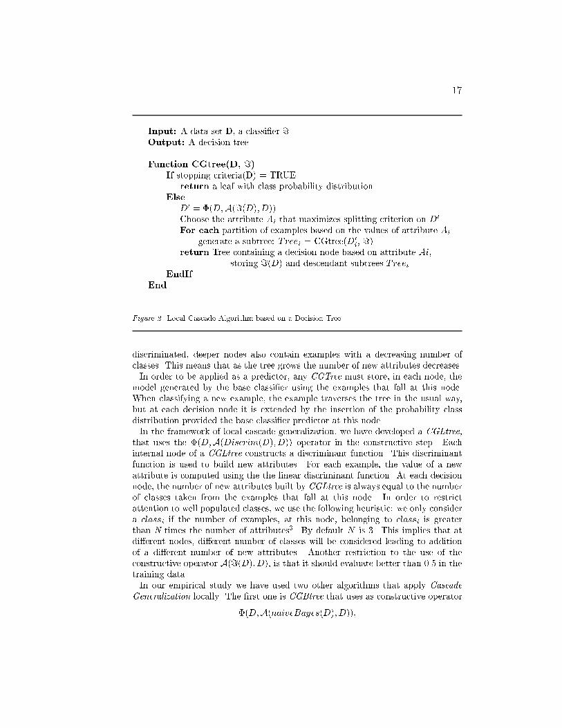
17Input: A data set D, a classi�er =Output: A decision treeFunction CGtree(D, =)If stopping criteria(D) = TRUEreturn a leaf with class probability distributionElseD0 = �(D;A(=(D); D))Choose the attribute Ai that maximizes splitting criterion on D0For each partition of examples based on the values of attribute Aigenerate a subtree: Treei = CGtree(D0i, =)return Tree containing a decision node based on attribute Ai,storing =(D) and descendant subtrees TreeiEndIfEndFigure 2. Local Cascade Algorithm based on a Decision Treediscriminated, deeper nodes also contain examples with a decreasing number ofclasses. This means that as the tree grows the number of new attributes decreases.In order to be applied as a predictor, any CGTree must store, in each node, themodel generated by the base classi�er using the examples that fall at this node.When classifying a new example, the example traverses the tree in the usual way,but at each decision node it is extended by the insertion of the probability classdistribution provided the base classi�er predictor at this node.In the framework of local cascade generalization, we have developed a CGLtree,that uses the �(D;A(Discrim(D); D)) operator in the constructive step. Eachinternal node of a CGLtree constructs a discriminant function. This discriminantfunction is used to build new attributes. For each example, the value of a newattribute is computed using the the linear discriminant function. At each decisionnode, the number of new attributes built by CGLtree is always equal to the numberof classes taken from the examples that fall at this node. In order to restrictattention to well populated classes, we use the following heuristic: we only considera classi if the number of examples, at this node, belonging to classi is greaterthan N times the number of attributes3. By default N is 3. This implies that atdi�erent nodes, di�erent number of classes will be considered leading to additionof a di�erent number of new attributes. Another restriction to the use of theconstructive operator A(=(D); D), is that it should evaluate better than 0.5 in thetraining data.In our empirical study we have used two other algorithms that apply CascadeGeneralization locally. The �rst one is CGBtree that uses as constructive operator�(D;A(naiveBayes(D); D)),

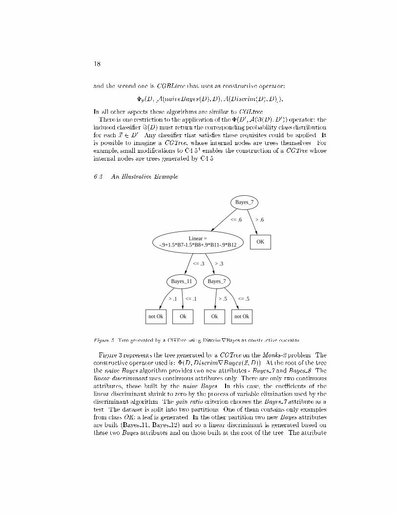
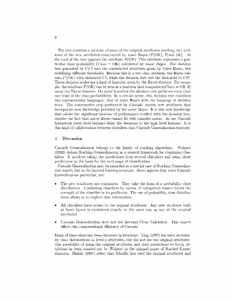
18and the second one is CGBLtree that uses as constructive operator:�p(D; [A(naiveBayes(D); D);A(Discrim(D); D)]),In all other aspects these algorithms are similar to CGLtree.There is one restriction to the application of the �(D0;A(=(D); D0)) operator: theinduced classi�er =(D) must return the corresponding probability class distributionfor each ~x 2 D0. Any classi�er that satis�es these requisites could be applied. Itis possible to imagine a CGTree, whose internal nodes are trees themselves. Forexample, small modi�cations to C4.54 enables the construction of a CGTree whoseinternal nodes are trees generated by C4.5.6.2. An Illustrative ExampleBayes_7

Linear =-.9+1.5*B7-1.5*B8+.9*B11-.9*B12

<= .6

OK

> .6

Bayes_11

<= .3

Bayes_7

> .3

not Ok

> .1

Ok

<= .1

Ok

> .5

not Ok

<= .5

Figure 3. Tree generated by a CGTree using DiscrimrBayes as constructive operatorFigure 3 represents the tree generated by a CGTree on the Monks-2 problem. Theconstructive operator used is: �(D;DiscrimrBayes(~x;D)). At the root of the treethe naive Bayes algorithm provides two new attributes - Bayes 7 and Bayes 8. Thelinear discriminant uses continuous attributes only. There are only two continuousattributes, those built by the naive Bayes. In this case, the coe�cients of thelinear discriminant shrink to zero by the process of variable elimination used by thediscriminant algorithm. The gain ratio criterion chooses the Bayes 7 attribute as atest. The dataset is split into two partitions. One of them contains only examplesfrom class OK: a leaf is generated. In the other partition two new Bayes attributesare built (Bayes 11, Bayes 12) and so a linear discriminant is generated based onthese two Bayes attributes and on those built at the root of the tree. The attribute

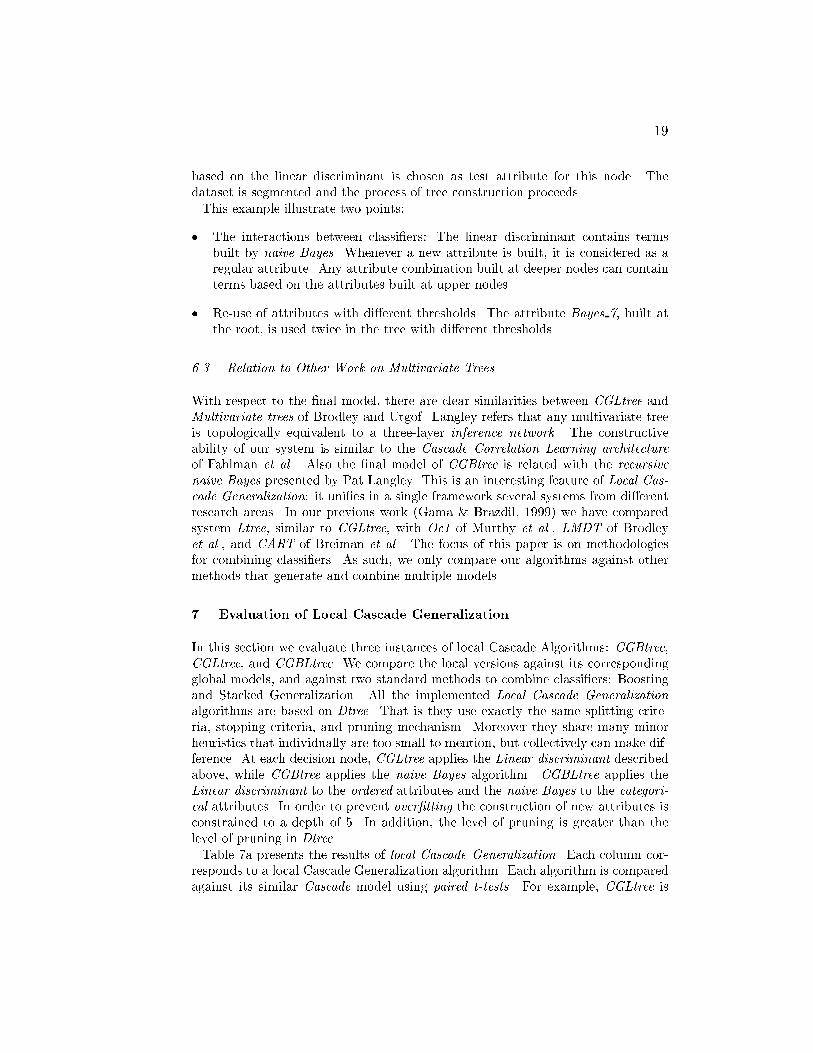
19based on the linear discriminant is chosen as test attribute for this node. Thedataset is segmented and the process of tree construction proceeds.This example illustrate two points:� The interactions between classi�ers: The linear discriminant contains termsbuilt by naive Bayes. Whenever a new attribute is built, it is considered as aregular attribute. Any attribute combination built at deeper nodes can containterms based on the attributes built at upper nodes.� Re-use of attributes with di�erent thresholds. The attribute Bayes 7, built atthe root, is used twice in the tree with di�erent thresholds.6.3. Relation to Other Work on Multivariate TreesWith respect to the �nal model, there are clear similarities between CGLtree andMultivariate trees of Brodley and Utgof. Langley refers that any multivariate treeis topologically equivalent to a three-layer inference network. The constructiveability of our system is similar to the Cascade Correlation Learning architectureof Fahlman et al.. Also the �nal model of CGBtree is related with the recursivenaive Bayes presented by Pat Langley. This is an interesting feature of Local Cas-cade Generalization: it uni�es in a single framework several systems from di�erentresearch areas. In our previous work (Gama & Brazdil, 1999) we have comparedsystem Ltree, similar to CGLtree, with Oc1 of Murthy et al., LMDT of Brodleyet al., and CART of Breiman et al.. The focus of this paper is on methodologiesfor combining classi�ers. As such, we only compare our algorithms against othermethods that generate and combine multiple models.7. Evaluation of Local Cascade GeneralizationIn this section we evaluate three instances of local Cascade Algorithms: CGBtree,CGLtree, and CGBLtree. We compare the local versions against its correspondingglobal models, and against two standard methods to combine classi�ers: Boostingand Stacked Generalization. All the implemented Local Cascade Generalizationalgorithms are based on Dtree. That is they use exactly the same splitting crite-ria, stopping criteria, and pruning mechanism. Moreover they share many minorheuristics that individually are too small to mention, but collectively can make dif-ference. At each decision node, CGLtree applies the Linear discriminant describedabove, while CGBtree applies the naive Bayes algorithm. CGBLtree applies theLinear discriminant to the ordered attributes and the naive Bayes to the categori-cal attributes. In order to prevent over�tting the construction of new attributes isconstrained to a depth of 5. In addition, the level of pruning is greater than thelevel of pruning in Dtree.Table 7a presents the results of local Cascade Generalization. Each column cor-responds to a local Cascade Generalization algorithm. Each algorithm is comparedagainst its similar Cascade model using paired t-tests. For example, CGLtree is

20compared against C4.5rDiscrim. A +(�) sign means that the error rate of thecomposite model is, at statistically signi�cant levels, lower (higher) than the corre-spondent model. Table 8 presents a comparative summary of the results betweenlocal Cascade Generalization and the corresponding global models. It illustratesthe bene�ts of applying Cascade Generalization locally.Table 7. Results of (a)Local Cascade Generalization (b)Boosting and Stacked (c) Boostinga Cascade algorithmDataset CGBtree CGLtree CGBLtree C5.0Boost Stacked C5BrBayes(vs. Corresponding Cascade Models) (vs. CGBLtree) (vs. C5.0Boost)Adult 13.46�0.4 13.56�0.3 13.52�0.4 � 14.33�0.4 13.96�0.6 14.41�0.5Australian 14.45�0.7 � 14.69�0.9 13.95�0.7 13.21�0.7 13.99�0.4 13.96�0.9Balance 5.32�1.1 8.24�0.5 � 8.08�0.4 � 20.03�1.0 7.75�0.9 + 4.25�0.7Banding 20.98�1.2 23.60�1.2 20.69�1.2 + 17.39�1.7 21.45�1.2 18.38�1.8Breast(W) 2.62�0.1 + 3.23�0.4 2.66�0.1 � 3.34�0.3 2.66�0.1 3.03�0.2Cleveland + 15.10�1.4 + 16.54�0.8 16.50�0.8 � 18.95�1.3 16.75�0.9 17.86�1.1Credit 15.35�0.5 14.41�0.8 14.52�0.8 13.41�0.8 13.43�0.6 13.57�0.9Diabetes 25.37�1.5 24.43�0.9 24.48�0.9 24.58�0.9 23.62�0.4 24.71�1.1German 25.37�1.1 24.78�1.1 + 24.88�0.8 25.36�0.8 24.72�0.3 25.20�1.1Glass 32.08�2.5 34.71�2.3 32.35�2.0 + 25.06�2.0 31.28�1.8 � 29.23�1.6Heart + 16.37�1.0 16.85�1.2 + 16.81�1.1 � 19.94�1.3 16.19�0.9 + 17.24�1.5Hepatitis 16.87�1.1 + 16.87�1.1 16.87�1.1 16.67�1.5 15.33�1.1 15.93�1.3Ionosphere 9.62�0.9 11.06�0.6 11.00�0.7 + 6.57�1.1 9.63�1.2 7.71�0.7Iris 4.73�1.3 2.80�0.4 + 2.80�0.4 � 5.68�0.6 4.13�1.0 5.07�0.8Letter 13.47�0.9 12.97�0.9 + 13.06�0.9 + 5.16�0.4 + 11.91�0.7 � 6.91�0.5Monks-1 � 9.39�3.5 6.80�3.3 � 8.53�3.0 + 0.00�0.0 + 3.74�2.0 0.33�0.3Monks-2 � 14.87�3.3 33.19�1.7 11.88�3.3 � 35.76�1.0 � 32.87�0.0 + 3.64�1.7Monks-3 0.39�0.4 � 0.92�0.5 0.39�0.4 0.00�0.0 � 2.24�0.8 0.63�0.3Mushroom 0.22�0.1 � 0.96�0.1 � 0.24�0.0 + 0.00�0.0 � 2.93�0.0 0.01�0.0Satimage + 11.86�0.3 11.99�0.3 + 11.99�0.3 + 9.25�0.2 � 13.11�0.4 9.21�0.2Segment � 4.36�0.2 3.19�0.3 3.20�0.3 + 1.79�0.1 3.32�0.2 � 2.09�0.1Sonar 26.23�1.7 25.26�1.5 25.50�1.6 + 19.25�2.2 24.81�1.0 23.02�1.2Vehicle 28.75�0.8 21.21�0.9 + 21.32�0.9 � 23.71�0.7 � 27.72�0.8 24.29�1.3Votes 3.29�0.4 4.30�0.5 + 3.26�0.4 4.11�0.4 3.65�0.4 4.30�0.4Waveform 16.50�0.6 + 15.74�0.5 16.12�0.5 � 17.45�0.4 � 17.14�0.4 + 15.58�0.3Wine 2.31�0.6 + 1.20�0.6 + 1.20�0.6 � 3.45�1.0 2.23�0.9 2.94�0.7System CGBLtree has been compared against C5.0Boosting, a variance reductionmethod5 and against Stacked Generalization, a bias reduction method. Table 7bpresents the results of C5.0Boosting with the default parameter of 10, that is aggre-gating over 10 trees, and Stacked Generalization as it is de�ned in Ting (1997) anddescribed in an earlier section. Both Boosting and Stacked are compared againstCGBLtree, using paired t-tests with the signi�cance level set to 99.9%. A +(�) signmeans that Boosting or Stacked performs signi�cantly better (worse) than CG-BLtree. In this study, CGBLtree performs signi�cantly better than Stacked, in 6datasets and worse in 2 datasets.

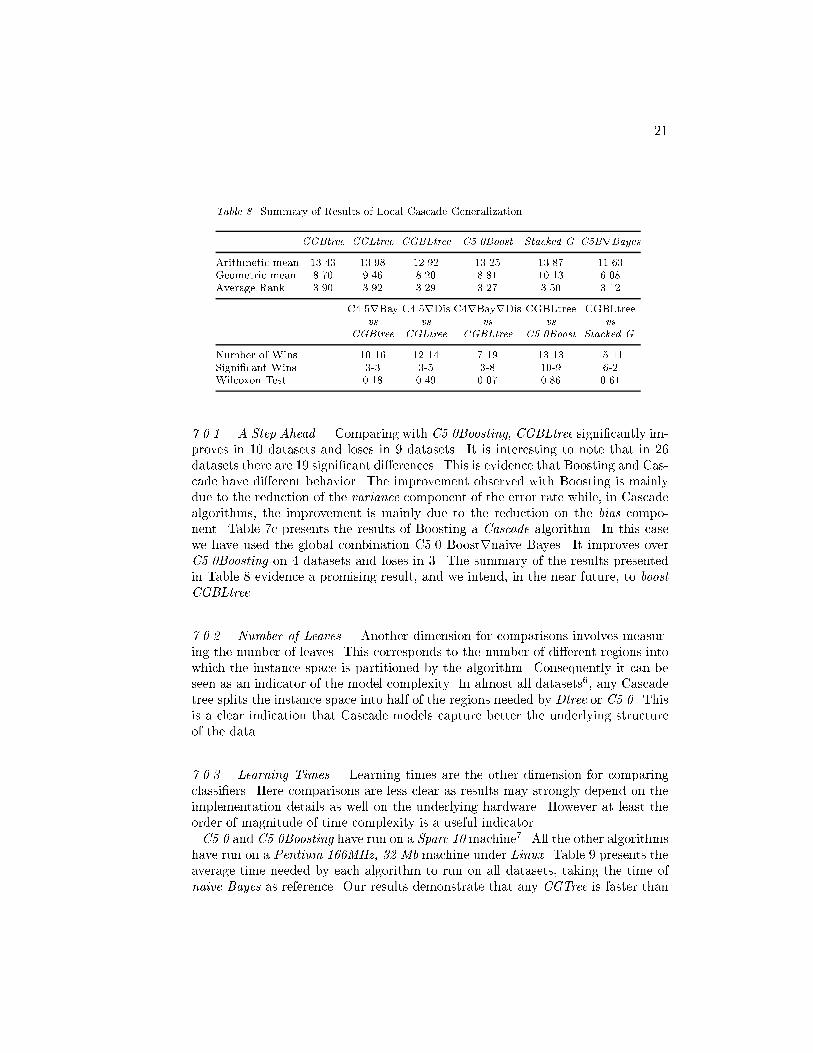
21Table 8. Summary of Results of Local Cascade Generalization.CGBtree CGLtree CGBLtree C5.0Boost Stacked G. C5BrBayesArithmetic mean 13.43 13.98 12.92 13.25 13.87 11.63Geometric mean 8.70 9.46 8.20 8.81 10.13 6.08Average Rank 3.90 3.92 3.29 3.27 3.50 3.12C4.5rBay C4.5rDis C4rBayrDis CGBLtree CGBLtreevs vs vs vs vsCGBtree CGLtree CGBLtree C5.0Boost Stacked G.Number of Wins 10-16 12-14 7-19 13-13 15-11Signi�cant Wins 3-3 3-5 3-8 10-9 6-2Wilcoxon Test 0.18 0.49 0.07 0.86 0.617.0.1. A Step Ahead. Comparing with C5.0Boosting, CGBLtree signi�cantly im-proves in 10 datasets and loses in 9 datasets. It is interesting to note that in 26datasets there are 19 signi�cant di�erences. This is evidence that Boosting and Cas-cade have di�erent behavior. The improvement observed with Boosting is mainlydue to the reduction of the variance component of the error rate while, in Cascadealgorithms, the improvement is mainly due to the reduction on the bias compo-nent. Table 7c presents the results of Boosting a Cascade algorithm. In this casewe have used the global combination C5.0 Boostrnaive Bayes. It improves overC5.0Boosting on 4 datasets and loses in 3. The summary of the results presentedin Table 8 evidence a promising result, and we intend, in the near future, to boostCGBLtree.7.0.2. Number of Leaves. Another dimension for comparisons involves measur-ing the number of leaves. This corresponds to the number of di�erent regions intowhich the instance space is partitioned by the algorithm. Consequently it can beseen as an indicator of the model complexity. In almost all datasets6, any Cascadetree splits the instance space into half of the regions needed by Dtree or C5.0. Thisis a clear indication that Cascade models capture better the underlying structureof the data.7.0.3. Learning Times. Learning times are the other dimension for comparingclassi�ers. Here comparisons are less clear as results may strongly depend on theimplementation details as well on the underlying hardware. However at least theorder of magnitude of time complexity is a useful indicator.C5.0 and C5.0Boosting have run on a Sparc 10 machine7. All the other algorithmshave run on a Pentium 166MHz, 32 Mb machine under Linux. Table 9 presents theaverage time needed by each algorithm to run on all datasets, taking the time ofnaive Bayes as reference. Our results demonstrate that any CGTree is faster than

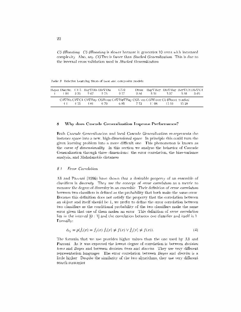
22C5.0Boosting. C5.0Boosting is slower because it generates 10 trees with increasedcomplexity. Also, any CGTree is faster than Stacked Generalization. This is due tothe internal cross validation used in Stacked Generalization.Table 9. Relative Learning times of base and composite modelsBayes Discrim C4.5 BayrDis DisrDis C5.0 Dtree BayrBay DisrBay BayrC4 DisrC41 1.04 2.35 2.67 2.75 2.77 2.86 3.31 3.37 3.59 3.65C4rDis C4rC4 C4rBay CGBtree C4rDisrBay CGLtree CGBLtree C5.0Boost Stacked4.1 4.55 4.81 6.70 6.85 7.72 11.08 15.16 15.298. Why does Cascade Generalization Improve Performance?Both Cascade Generalization and local Cascade Generalization re-represents theinstance space into a new, high-dimensional space. In principle this could turn thegiven learning problem into a more di�cult one. This phenomenon is known asthe curse of dimensionality. In this section we analyze the behavior of CascadeGeneralization through three dimensions: the error correlation, the bias-varianceanalysis, and Mahalanobis distances.8.1. Error CorrelationAli and Pazzani (1996) have shown that a desirable property of an ensemble ofclassi�ers is diversity. They use the concept of error correlation as a metric tomeasure the degree of diversity in an ensemble. Their de�nition of error correlationbetween two classi�ers is de�ned as the probability that both make the same error.Because this de�nition does not satisfy the property that the correlation betweenan object and itself should be 1, we prefer to de�ne the error correlation betweentwo classi�ers as the conditional probability of the two classi�ers make the sameerror given that one of them makes an error. This de�nition of error correlationlies in the interval [0 : 1] and the correlation between one classi�er and itself is 1.Formally:�ij = p(f̂i(x) = f̂j(x)jf̂i(x) 6= f(x) _ f̂j(x) 6= f(x)): (4)The formula that we use provides higher values than the one used by Ali andPazzani. As it was expected the lowest degree of correlation is between decisiontrees and Bayes and between decision trees and discrim. They use very di�erentrepresentation languages. The error correlation between Bayes and discrim is alittle higher. Despite the similarity of the two algorithms, they use very di�erentsearch strategies.

23Table 10. Error Correlation between base classi�ersC4 vs. Bayes C4 vs.Discrim Bayes vs. DiscrimAverage 0.32 0.32 0.40This results provide evidence that the decision tree and any discriminant functionmake uncorrelated errors, that is each classi�er make errors in di�erent regions ofthe instance space. This is a desirable property for combining classi�ers.8.2. Bias-Variance DecompositionThe bias-variance decomposition of the error is a tool from the statistics theory foranalyzing the error of supervised learning algorithms.The basic idea, consists on decomposing the expected error into three components:E(C) =Xx P (x)(�2 + bias2x + variancex) (5)where, the bias measures how closely the learning algorithm's average guess matchesthe target. It is computed as:bias2x = 12Xy2Y (P (YF = y)� P (YH = y))2 (6)where, the variance measures how much the learning algorithm's guess \bouncesaround" for the di�erent sets of the given size. This is computed as:variancex = 12(1�Xy2Y P (YH = y)2) (7)Equations 6 and 7 for zero-one loss functions are not consensual. We use thedecomposition proposed by Kohavi and Wolpert (1996).To estimate the bias and variance, we �rst split the data into training and testsets. From the training set we obtain ten bootstrap replications used to buildten classi�ers. We ran the learning algorithm on each of the training sets andestimated the terms of the variance equation 7 and bias8 equation 6 using thegenerated classi�er for each point x in the evaluation set E. All the terms wereestimated using frequency counts.The base algorithms used in the experimental evaluation have di�erent behaviorunder a Bias-Variance analysis. A decision tree is known to have low bias but highvariance, and naive Bayes and linear discriminant are known to have low variancebut high bias.

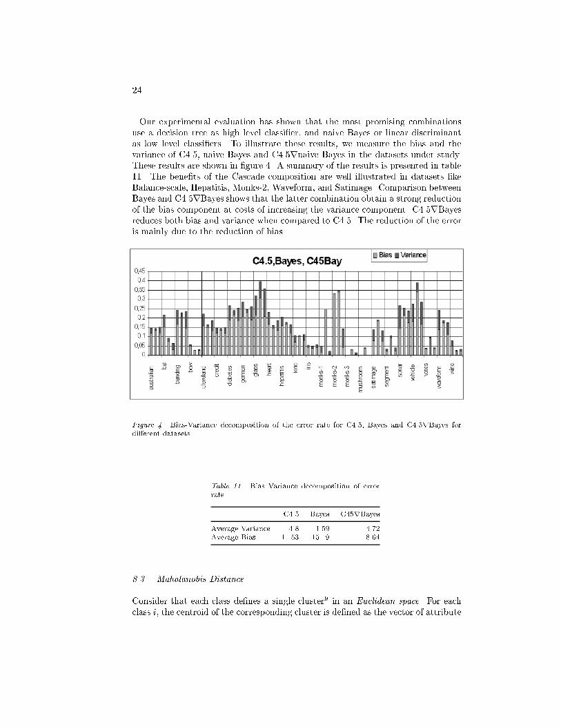
24Our experimental evaluation has shown that the most promising combinationsuse a decision tree as high level classi�er, and naive Bayes or linear discriminantas low level classi�ers. To illustrate these results, we measure the bias and thevariance of C4.5, naive Bayes and C4.5rnaive Bayes in the datasets under study.These results are shown in �gure 4. A summary of the results is presented in table11. The bene�ts of the Cascade composition are well illustrated in datasets likeBalance-scale, Hepatitis, Monks-2, Waveform, and Satimage. Comparison betweenBayes and C4.5rBayes shows that the latter combination obtain a strong reductionof the bias component at costs of increasing the variance component. C4.5rBayesreduces both bias and variance when compared to C4.5. The reduction of the erroris mainly due to the reduction of bias.

Figure 4. Bias-Variance decomposition of the error rate for C4.5, Bayes and C4.5rBayes fordi�erent datasets. Table 11. Bias Variance decomposition of errorrate C4.5 Bayes C45rBayesAverage Variance 4.8 1.59 4.72Average Bias 11.53 15.19 8.648.3. Mahalanobis DistanceConsider that each class de�nes a single cluster9 in an Euclidean space. For eachclass i, the centroid of the corresponding cluster is de�ned as the vector of attribute

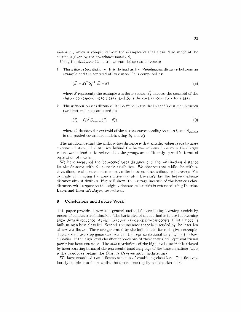
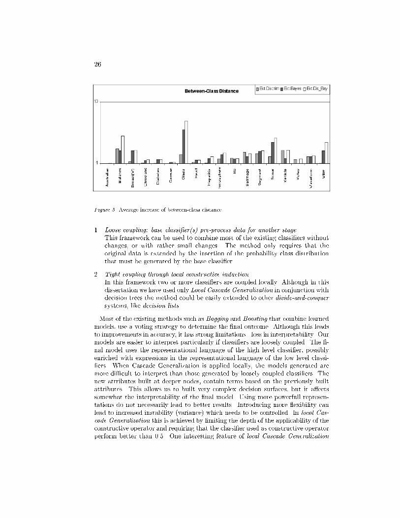
25means �xi, which is computed from the examples of that class. The shape of thecluster is given by the covariance matrix Si.Using the Mahalanobis metric we can de�ne two distances:1. The within-class distance. It is de�ned as the Mahalanobis distance between anexample and the centroid of its cluster. It is computed as:(~�xi � ~x)TS�1i (~�xi � ~x) (8)where ~x represents the example attribute vector, ~�xi denotes the centroid of thecluster corresponding to class i, and Si is the covariance matrix for class i.2. The between-classes distance. It is de�ned as the Mahalanobis distance betweentwo clusters. It is computed as:(~�xi � ~�xj)TS�1pooled(~�xi � ~�xj) (9)where ~�xi denotes the centroid of the cluster corresponding to class i, and Spooledis the pooled covariance matrix using Si and Sj .The intuition behind the within-class distance is that smaller values leads to morecompact clusters. The intuition behind the between-classes distance is that largervalues would lead us to believe that the groups are su�ciently spread in terms ofseparation of means.We have measured the between-classes distance and the within-class distancefor the datasets with all numeric attributes. We observe that while the within-class distance almost remains constant the between-classes distance increases. Forexample when using the constructive operator DiscrimrBay the between-classesdistance almost doubles. Figure 5 shows the average increase of the between-classdistance, with respect to the original dataset, when this is extended using Discrim,Bayes and DiscrimrBayes, respectively.9. Conclusions and Future WorkThis paper provides a new and general method for combining learning models bymeans of constructive induction. The basic idea of the method is to use the learningalgorithms in sequence. At each iteration a two step process occurs. First a model isbuilt using a base classi�er. Second, the instance space is extended by the insertionof new attributes. These are generated by the built model for each given example.The constructive step generates terms in the representational language of the baseclassi�er. If the high level classi�er chooses one of these terms, its representationalpower has been extended. The bias restrictions of the high level classi�er is relaxedby incorporating terms of the representational language of the base classi�ers. Thisis the basic idea behind the Cascade Generalization architecture.We have examined two di�erent schemes of combining classi�ers. The �rst oneloosely couples classi�ers whilst the second one tightly couples classi�ers.

26

Figure 5. Average increase of between-class distance.1. Loose coupling: base classi�er(s) pre-process data for another stageThis framework can be used to combine most of the existing classi�ers withoutchanges, or with rather small changes. The method only requires that theoriginal data is extended by the insertion of the probability class distributionthat must be generated by the base classi�er.2. Tight coupling through local constructive inductionIn this framework two or more classi�ers are coupled locally. Although in thisdissertation we have used only Local Cascade Generalization in conjunction withdecision trees the method could be easily extended to other divide-and-conquersystems, like decision lists.Most of the existing methods such as Bagging and Boosting that combine learnedmodels, use a voting strategy to determine the �nal outcome. Although this leadsto improvements in accuracy, it has strong limitations - loss in interpretability. Ourmodels are easier to interpret particularly if classi�ers are loosely coupled. The �-nal model uses the representational language of the high level classi�er, possiblyenriched with expressions in the representational language of the low level classi-�ers. When Cascade Generalization is applied locally, the models generated aremore di�cult to interpret than those generated by loosely coupled classi�ers. Thenew attributes built at deeper nodes, contain terms based on the previously builtattributes. This allows us to built very complex decision surfaces, but it a�ectssomewhat the interpretability of the �nal model. Using more powerfull represen-tations do not necessarily lead to better results. Introducing more exibility canlead to increased instability (variance) which needs to be controlled. In local Cas-cade Generalization this is achieved by limiting the depth of the applicability of theconstructive operator and requiring that the classi�er used as constructive operatorperform better than 0.5. One interesting feature of local Cascade Generalization

27is that it provides a single framework, for a collection of di�erent methods. Ourmethod can be related to several paradigms of machine learning. For example thereare similarities with multivariate trees (Brodley & Utgof, 1995), neural networks(Fahlman & Lebiere, 1990), recursive Bayes (Langley, 1993), and multiple mod-els, namely Stacked Generalization (Wolpert, 1992). In our previous work (Gama& Brazdil, 1999) we have presented system Ltree that combines a decision treewith a discriminant function by means of constructive induction. Local Cascadecombinations extend this work. In Ltree the constructive operator was a single dis-criminant function. In Local Cascade composition this restriction was relaxed. Wecan use any classi�er as constructive operator. Moreover, a composition of severalclassi�ers, like in CGBLtree, could be used.The uni�ed framework is useful because it overcomes some super�cial distinctionsand enables us to study more fundamental ones. From a practical perspectivethe user's task is simpli�ed, because his aim of achieving better accuracy can beachieved with a single algorithm instead of several ones. This is done e�cientlyleading to reduced learning times.We have shown that this methodology can improve the accuracy of the baseclassi�ers, competing well with other methods for combining classi�ers, preservingthe ability to provide a single, albeit structured model for the data.9.1. Limitations and Future WorkSome open issues, which could be explored in future, involve:� From the perspective of bias-variance analysis the main e�ect of the proposedmethodology is a reduction on the bias component. It should be possible tocombine the Cascade architecture with a variance reduction method, like Bag-ging or Boosting.� Will Cascade Generalization work with other classi�ers? Could we use neuralnets or nearest neighbors? We think that the methodology presented will workfor this type of classi�ers. We intend to verify it empirically in future.Other problems that involve basic research include:� Why does Cascade Generalization improve performance?Our experimental study suggests that we should combine algorithms with com-plementary behavior from the point of view of bias-variance analysis. Otherforms of complementarity can be considered, for example the search bias. So,one interesting issue to be explored is: given a dataset, can we predict whichalgorithms are complementary?� When does Cascade Generalization improve performance?In some datasets Cascade was not able to improve the performance of baseclassi�ers. Can we characterize these datasets? That is, can we predict un-der what circumstances Cascade Generalization will lead to an improvement inperformance?

28� How many base classi�ers should we use?The general preference is for smaller number of base classi�ers. Under whatcircumstances can we reduce the number of base classi�ers without a�ectingperformance?� The Cascade Generalization architecture provides a method for designing algo-rithms that use multiple representations and multiple search strategies withinthe induction algorithm. An interesting line of future research should explore exible inductive strategies using several diverse representations. It should bepossible to extend local Cascade Generalization to provide a dynamic controland this make a step in this direction.AcknowledgmentsGratitude is expressed to the �nancial support given by the FEDER and PRAXISXXI projects, projects ECO and METAL, and the Plurianual support attributed toLIACC. Thanks to the anonymous reviewers, Pedro Domingos and my colleaguesfrom LIACC for the valuable comments.Notes1. Except in the case of Adult and Letter datasets, where a single 10-fold cross-validation wasused.2. We have also evaluated Stacked Generalization using C4.5 at top level. The version that wehave used is somewhat better. Using C4.5 at top level the average mean of the error rate is15.14.3. This heuristic was suggested by Breiman et al.4. Two di�erent methods are presented in Ting (1997) and Gama (1998).5. We have preferred C5.0Boosting (instead of Bagging) because it is available for us and allowscross-checking of the results. There are some di�erences between our results and those previouspublished by Quinlan. We think that this may be due to the di�erent methods used to estimatethe error rate.6. Except on Monks-2 dataset, where both Dtree and C5.0 produce a tree with only one leaf.7. The running time of C5.0 and C5.0Boosting were reduced by a factor of 2 as suggested in:www.spec.org.8. The intrinsic noise in the training dataset will be included in the bias term.9. This analysis assumes that there is a single dominant class for each cluster. Although this maynot always be satis�ed, it can give insights about the behavior of Cascade composition.References11K. Ali and M. Pazzani. Error reduction through learning multiple descriptions. Machine Learning,Vol. 24, No. 1, 1996.Eric Bauer and Ron Kohavi. An empirical comparison of voting classi�cation algorithms: Bagging,boosting, and variants. Machine Learning, 36:105{139, 1999.L. Breiman. Arcing classi�ers. The Annals of Statistics, 26(3):801{849, 1998.

29L. Breiman, J. Friedman, R. Olshen, and C. Stone. Classi�cation and Regression Trees. WadsworthInternational Group., 1984.Carla E. Brodley. Recursive automatic bias selection for classi�er construction. Machine Learning,20:63{94, 1995.Carla E. Brodley and Paul E. Utgo�. Multivariate decision trees. Machine Learning, 19:45{77,1995.Wray Buntine. A theory of Learning Classi�cation Rules. PhD thesis, University of Sydney,1990.P. Chan and S. Stolfo. A comparative evaluation of voting and meta-learning on partitioned data.In A. Prieditis and S. Russel, editors, Machine Learning Proc of 12th International Conference.Morgan Kaufmann, 1995.P. Chan and S. Stolfo. Learning arbiter and combiner trees from partitioned data for scalingmachine learning. In KDD 95, 1995.W. Dillon and M. Goldstein. Multivariate Analysis, Methods and Applications. J. Wiley andSons, Inc., 1984.Pedro Domingos and Michael Pazzani. On the optimality of the simple bayesian classi�er underzero-one loss. Machine Learning, 29:103{129, 1997.J. Dougherty, R. Kohavi, and M. Sahami. Supervised and unsupervised discretization of con-tinuous features. In A. Prieditis and S. Russel, editors, Machine Learning Proc. of 12thInternational Conference. Morgan Kaufmann, 1995.Scott E. Fahlman and Christian Lebiere. The recurrent cascade-correlation architecture. InRichard P. Lippmann, John E. Moody, and David S. Touretzky, editors, Advances in NeuralInformation Processing Systems, volume 3, pages 190{196. Morgan Kaufmann Publishers, Inc.,1991.Yoav Freund and Robert E. Schapire. Experiments with a new boosting algorithm. In L. Saitta,editor,Machine Learning, Proceedings of the 13th International Conference. Morgan Kaufmann,1996.J. Gama. Combining classi�ers by constructive induction. In C. Nedellec and C. Rouveirol,editors, Machine Learning ECML-98. Springer Verlag, 1998.J. Gama and P. Brazdil. Linear tree. Intelligent Data Analysis, 3(1), 1999.B. Henery. Combining classi�cation procedures. In C. Taylor R. Nakhaeizadeh, editor, MachineLearning and Statistics. The Interface. John Wiley, Sons, Inc., 1997.R Kohavi and D. Wolpert. Bias plus variance decomposition for zero-one loss function. InL. Saitta, editor,Machine Learning Proc. of 13th International Conference. Morgan Kaufmann,1996.P. Langley. Induction of recursive bayesian classi�ers. In P.Brazdil, editor, Machine Learning:ECML-93. LNAI 667, Springer Verlag, 1993.Pat Langley. Elements of Machine Learning. Morgan Kaufmann, 1996.D. Michie, D.J. Spiegelhalter, and C. Taylor. Machine Learning, Neural and Statistical Classi�-cation. Ellis Horwood, 1994.Tom Mitchell. Machine Learning. MacGraw-Hill Companies, Inc., 1997.S. Murthy, S. Kasif, and S. Salzberg. A system for induction of oblique decision trees. Journalof Arti�cial Intelligence Research, 1994.J. Pearl. Probabilistic Reasoning in Intelligent Systems: Networks of Plausible Inference. MorganKaufmann Publishers, Inc., 1988.R. Quinlan. Bagging, boosting and c4.5. In Procs. 13th American Association for Arti�cialIntelligence. AAAI Press, 1996.Ronald L. Rivest. Learning decision lists. Machine Learning, 2:229{246, 1987.David Skalak. Prototype Selection For Composite Nearest Neighbor Classi�ers. PhD thesis,University of Massachusetts Amherst, 1997.S. Thrun and et all. The monk's problems: A performance comparison of di�erent learningalgorithms. Technical Report CMU-CS-91-197, 1991.K.M. Ting and I.H. Witten. Stacked generalization: when does it work? In Procs. InternationalJoint Conference on Arti�cial Intelligence. Morgan Kaufmann, 1997.K. Tumer and J. Ghosh. Classi�er combining: analytical results and implications. In AAAI 96 -Workshop in Induction of Multiple Learning Models, 1995.D. Wolpert. Stacked generalization. In Pergamon Press, editor, Neural Networks Vol.5, 1992.