Stoichiometry in Producer-Grazer Systems: Linking Energy Flow with Element Cycling

Available online at http://www.idealibrary.com ondoi:10.1006/bulm.2000.0201Bulletin of Mathematical Biology(2000)62, 1137–1162

Stoichiometry in Producer–Grazer Systems: LinkingEnergy Flow with Element Cycling

IRAKLI LOLADZE AND YANG KUANG

Department of Mathematics,

Arizona State University,Tempe, AZ 85287-1804, U.S.A.E-mail: [email protected]

E-mail: [email protected]

JAMES J. ELSER

Department of Biology,

Arizona State University,Tempe, AZ 85287-1501l, U.S.A.E-mail: [email protected]

All organisms are composed of multiple chemical elements such as carbon, nitro-gen and phosphorus. Whileenergy flowandelement cyclingare two fundamentaland unifying principles in ecosystem theory, population models usually ignore thelatter. Such models implicitly assume chemical homogeneity of all trophic lev-els by concentrating on a single constituent, generally an equivalent of energy. Inthis paper, we examine ramifications of an explicit assumption that both producerand grazer are composed of two essential elements: carbon and phosphorous. Us-ing stoichiometric principles, we construct a two-dimensional Lotka–Volterra typemodel that incorporates chemical heterogeneity of the first two trophic levels ofa food chain. The analysis shows that indirect competition between two popula-tions for phosphorus can shift predator–prey interactions from a(+,−) type toan unusual(−,−) class. This leads to complex dynamics with multiple positiveequilibria, where bistability and deterministic extinction of the grazer are possible.We derive simple graphical tests for the local stability of all equilibria and showthat system dynamics are confined to a bounded region. Numerical simulationssupported by qualitative analysis reveal that Rosenzweig’s paradox of enrichmentholds only in the part of the phase plane where the grazer is energy limited; a newphenomenon, the paradox of energy enrichment, arises in the other part, where thegrazer is phosphorus limited. A bifurcation diagram shows that energy enrichmentof producer–grazer systems differs radically from nutrient enrichment. Hence, ex-pressing producer–grazer interactions in stoichiometrically realistic terms revealsqualitatively new dynamical behavior.

c© 2000 Society for Mathematical Biology

0092-8240/00/061137 + 26 $35.00/0 c© 2000 Society for Mathematical Biology

1138 I. Loladzeet al.

1. INTRODUCTION

Energy flow through trophic levels is a fundamental and unifying principle inecosystem science (Odum, 1968; Reiners, 1986; Hagen, 1992). It is based on twoideas. First, this approach separates an ecosystem into distinct trophic levels. Thefirst level aggregates all biomass that transforms solar energy into a usable chem-ical form, i.e., primary producers (hereafter, producers). The next level comprisesall organisms directly feeding on producers, i.e., herbivores or grazers. Carnivores,feeding on herbivores, are the third level, and so on. The other idea is that energymust dissipate as it flows through this vertical structure due to the second law ofthermodynamics. Hence, as energy is transferred from one trophic level into thenext, some part of it must be lost, forcing ecological transfer efficiency or produc-tion efficiency to be less than 100%.

Usually, population dynamics models assume a constant production efficiency,as in the classical Lotka–Volterra equations, which succinctly utilize the energyflow principle:

dx

dt= bx− f (x)y (1a)

dy

dt= ef(x)y− dy. (1b)

Here the system is divided into two trophic levels, prey and predator (x andy aretheir respective densities or biomasses in the same units) and the yield constant orthe production efficiency(e), manifests the second law of thermodynamics(0 ≤e < 1). Sincee is a constant and the functional response of the predator,f (x),is a monotone non-decreasing function, it follows that higher prey density neverlowers predator growth rate. In other words, energy enrichment of the first trophiclevel never decreases the flow of energy to the next level. In fact, all predator–prey relationships are considered as a (+,−) type, as indicated by the signs of theoff-diagonal terms in the community matrix or Jacobian of system (1).

In the above discussion we used the terminology of energetics and never men-tioned chemical elements. However, in reality, energy flow in a food web is intri-cately bound to chemical elements. Solar energy, once transformed by producers,flows through an ecosystem only as chemical energy in covalent bonding betweenvarious elements in organic compounds. Furthermore, organisms build themselvesfrom a variety of essential nutrients such as carbon, nitrogen, phosphorous, sulfur,and calcium. Can the demand of organisms for multiple nutrients alter energy flowand predator–prey interactions in a way not accounted for by energetics consid-erations? Recent experiments involving zooplankton–phytoplankton interactionsshow that it can.

Urabe and Sterner (1996) grew algae (a producer) at different light intensities inbatch cultures. The systems were open for light energy and carbon that entered

Stoichiometry in Producer–Grazer Systems 1139

the system from air as CO2. Phosphorus was limited while all other nutrients werepresent in abundance. As light input was increased, algal density increased throughthe entire range of light intensity. One would expect that the growth rate of zoo-plankton grazing on the algae would positively correlate with algal density. Thisindeed happened, but only from low to intermediate light levels. Further increasesin light intensity resulted in yet higher algal density but lower animal growth rates.Why did high food density hurt the grazer growth rate? One cannot explain thisparadoxical result in energy terms without makingad hocassumptions. However,Urabe and Sternergave a simple explanation involving the stoichiometry of twoessential elements, carbon and phosphorous.

At higher light intensity, algae increased photosynthetic fixation of carbon. Sincethe quantity of phosphorus in the system was limited, this led to lower phospho-rous to carbon ratio (P:C) in algal biomass. However, zooplankton physiologydoes not allow significant variation in body P:C ratio. This is a rather generalproperty among consumer species. Thus, a growing grazer must maintain a spe-cific chemical composition of its body (Andersen and Hessen, 1991; Sterner andHessen, 1994). If the P:C in algal biomass becomes lower than the zooplankton’sspecific P:C ratio, then the grazer cannot utilize the excess energy (carbon) ac-quired from algae and simply excretes or egests it. In other words, under high lightenergy input, algae becomelow quality foodfor the grazer lowering the productionefficiency in carbon terms [simultaneously, the grazer’s assimilation of phosphorusincreases;Elser and Urabe (1999)]. These and other results demonstrate that massbalance of multiple chemical elements can affect trophic dynamics (Elseret al.,1998; Sterneret al., 1998). However, current ecological theory fails to stress closeconnections between the cycling of chemical elements and the flow of energy infood webs. Possibly, the reason lies in the historical development of energy flowconcepts and population dynamics theory.

Lotka (1925) pioneered thermodynamic applications in ecology in his book ‘El-ements of Mathematical Biology’, the same book where he introduced and anal-ysed predator–prey equations. In the chapter ‘The Energy Transformers of Nature’,Lotka wrote that the main variables in his general equations, ‘aggregates of livingorganisms—are, in their physical relations,energy transformers’. As energy flowsthrough the system, a fraction of it is lost because ‘the second law of thermo-dynamics inexorably demands this payment of a tax to nature’. However, Lotkadid not limit himself to applications of energetics principles to ecology and envi-sioned how additional physical-chemical laws might affect ecological dynamics.He stressed that living matter is not a homogeneous substance for energy transfor-mation and storage, but instead is composed of multiple chemical elements: eachenergy transformer ‘does not operate with a single working substance, but witha complex variety of such substances, a fact which has certain important conse-quences’. Therefore, Lotka thoroughly analysed and compared the ratios of essen-tial chemical elements in organisms and their abiotic environment, one of the firstapplications of its kind. Furthermore, he used a special term, ‘stoichiometry’, to


denote ‘that branch of the science which concerns itself with material transforma-tions, with the relations between the masses of the components’.

Unfortunately, Lotka’s work in the area of stoichiometry did not gain much pop-ularity among ecologists. Instead, it wasLindeman’s (1942) classic paper, ‘Thetrophic-dynamic aspect of ecology’, that brought new meaning to ecosystem sci-ence. Lindeman separated lake communities into distinct trophic levels: phyto-plankton, zooplankton, plankton predators and swimming predators. Using fielddata, he quantified energy transfer efficiencies between trophic levels. Like Lotka,Lindeman saw intricate connections between energy and nutrients and used thesame arrows to denote both energy and nutrient flows on his famous diagram. Lin-deman even discussed how the ratio of two essential elements, nitrogen to phos-phorus (N:P), affects lake productivity. However, Lindeman’s work is primarilyremembered in the context of energy flow in food chains. Subsequent events sawincreasing separation of energy flow and biogeochemical cycling as distant phe-nomena to be studied separately.

In the next decade Howard Odum (1957, 1960), drawing parallels between eco-logical, physical and electrical systems, isolated energy from nutrients and createdunambiguous pure energy flow diagrams. Concentrating on energy allowed him toavoid complications and confusion with recycling. Unlike nutrients, energy, oncelost in respiration, cannot be recycled and therefore, flows through trophic levelsunidirectionally. The convenience of such single common currency for an entiresystem became apparent to ecologists. Indeed, Howard’s brother, EugeneOdum(1959), made energy flow diagrams part of his influential ‘Theoretical Ecology’book. It can be argued that from there, the energy flow concept, largely divorcedfrom element cycling, has had a preeminent place in discussion of food web dy-namics.

Has this development of energy flow principles influenced population dynamicstheory? Consider that 70 years of development of the Lotka–Volterra equations hasenhanced them with age, size and spatial heterogeneity. However, for the originatorof this equations, Lotka, another kind of heterogeneity, ‘chemical heterogeneity’,was more important. It is ironic that this direction has not received much attentionuntil very recently.

Recent advances in stoichiometric theory have revived Lotka’s work. Extendinggeneral approaches of resource ratio competition theory (Tilman, 1982), Sterner(1990), Hessen and Andersen (1992), Elseret al. (1998) andDeMott (1998) haveinvestigated stoichiometric effects on algae–zooplankton interactions.Andersen(1997) explicitly used stoichiometric constraints in modeling the dynamics ofpelagic systems; in particular, the assimilation efficiency of zooplankton in hismodel depends on nutrient content of phytoplankton. Kooijman’s (2000) dynamicenergy and mass budgets theory encompasses energy and nutrient fluxes on cellu-lar, organismal and population levels. We refer readers toElser and Urabe (1999)for a review of recent progress in stoichiometric nutrient recycling theory and po-tential new directions proposed by these authors.


The simple two-dimensional Lotka–Volterra model (1) captures the essence ofthe energy flow principle, yet all vestiges of stoichiometric reality are absent. Inthis paper we build stoichiometric principles into Lotka–Volterra equations with aminimum of added complexity. As in the above described experiments, we are pri-marily interested in effects of light energy enrichment of producer–grazer systems.However, analytical and numerical analyses of the resulting model (Sections3and4) provide more insight into system dynamics. For example, bifurcation anal-ysis reveals qualitative differences in the effects of energy and nutrient enrichmenton trophic dynamics.

2. MODEL CONSTRUCTION

In our qualitative model we concentrate on the first two trophic levels of a foodchain, where the prey is a primary producer and the predator is a grazer. Sincewe will be drawing parallels with the above described experiments we can think ofthe producer as phytoplankton (algae) and the grazer as zooplankton (for example,Daphnia), both placed in a clear flask in a constantly stirred culture. Our simpleecosystem is open for light energy and carbon, which freely enters the system fromthe atmosphere for fixation by the producer. We will express our assumptions aboutother nutrients later in this section.

We start the model construction with the Rosenzweig–MacArthur variation ofLotka–Volterra equations as applied to our spatially homogeneous system:

dx

dt= bx

(1−

x

K

)− f (x)y (2a)

dy

dt= ef(x)y− dy, (2b)

where

x is the density of producer (in milligrams of carbon per liter, mg C l−1),y is the density of grazer (mg C l−1).b is the intrinsic growth rate of producer (day−1),d is the specific loss rate of grazer that includes metabolic losses (respiration)

and death (day−1).f (x) is the grazer’s ingestion rate, which we take here as a Holling type II func-

tional response. In other words,f (x) is a bounded smooth function thatsatisfies the following assumptions:

f (0) = 0, f ′(x) > 0, f ′(0) <∞ and f ′′(x) < 0 for x ≥ 0. (3)


The choice of Holling type II function is largely for convenience. For most of theanalysis that follows, one can choose Holling type I and III functional responses aswell, though they may occasionally make analytical derivations more tedious.

The parameterse andK require special consideration and will undergo signifi-cant changes before we arrive at our terminal model (6). In model (2):

(a) e is aconstantproduction efficiency (yield constant). This is the conversionrate of ingested food into grazer biomass. The basic model (2) is purely energetic inthe sense that producer and grazer densities are given in energy equivalents. Suchan approach makes the producer always of the same quality for the grazer andleaves no natural and internal mechanism to introduce food quality. In reality, theprocess of food assimilation is an extremely complex process that depends stronglyon the quality of ingested food, which in turn depends on nutrient availability.Reducing such a complicated conversion to a single constante is a weakness inmany predator–prey models.

(b) K is the producer’sconstantcarrying capacity that depends on some externalfactors bounding its density. The only controlled external factor for our systemis light intensity. Suppose that we fix light intensity at a certain value and let theproducer grow without the grazer and with ample nutrients. Then producer densitywill increase until self-shading ultimately stabilizes it at some value,K . While Kis independent of any internal factors it positively correlates with light intensity ashigher light input (that is, below photoinhibition level) allows the producer to reachhigher density. What if some nutrient becomes limiting and a grazer is present inthe system? Can such internal factors affect carrying capacity? In the more generalcontext of population dynamics, is it a sound modeling practice to tie the upperbound of population density to a single constant?

Incorporation of stoichiometric reality into the model naturally resolves theseproblems. So let us proceed to this step, with our assumptions below.

Any form of life on the Earth builds itself out of various essential elements suchas carbon, nitrogen, phosphorus, calcium, sulfur and potassium. We will trackonly two essential substances, carbon and phosphorus. We assume that all othernutrients are abundant in the system and that their content in producer biomass doesnot limit grazer growth. Since the bulk of dry weight of most organisms is carbon,we express biomass of the populations in carbon terms. There is nothing particularwith the choice of phosphorus; any essential nutrient can be considered instead. Wechose phosphorus because it is frequently a limiting nutrient in freshwater systems(Schindler, 1977; Elseret al., 1990) and was limiting to both algae and grazers inthe experiments ofUrabe and Sterner (1996), andSterneret al. (1998). What isimportant is that we introduce a second ‘working substance’.

ASSUMPTION 1. The total mass of phosphorus in the entire system is fixed, i.e.,the system is closed for phosphorus with a total of P (mg P l−1).

The following important stoichiometric principles lead to the next assumption.Every organism requires at least a certain, species-specific, fraction of phosphorus


in their biomass. We say ‘at least’, because in producers P:C can vary significantlywithin a species. For example, the green algaScenedesmus acutuscan have cellularP:C ratios (by mass) that range from 1.6× 10−3 to 13× 10−3. In animals, P:Cvaries much less within a species. For example,Daphnia’s somantic elementalcomposition appears to be homeostatically regulated within narrow bounds (P:Caround 31× 10−3 by mass), even when food P:C diverges strongly (Sterner andHessen, 1994).

ASSUMPTION 2. Phosphorus to carbon ratio (P:C) in the producer varies, butit never falls below a minimum q (mg P/mg C); the grazer maintains a constantP :C, θ (mg P/mg C).

ASSUMPTION 3. All phosphorus in the system is divided into two pools: phos-phorus in the grazer and phosphorus in the producer.

FollowingAndersen (1997), we assume immediate recycling of phosphorus fromexcreted and dead matter and its immediate utilization by the producer. Hence,there is no free, inorganic phosphorus pool. We will address the validity of thisassumption in the discussion section. Here, we only mention that in most freshwa-ter systems the concentration of free phosphate in water is often very low or belowdetection because algae quickly absorb almost all available phosphorus.

Let us see how these three assumptions affect model (2). Light intensity limitsproducer density toK (mg C l−1). However, even in the absence of such an externallimitation, the combination of Assumptions1 and2 imposes another limit on theproducer,P/q (mg C l−1). Moreover, the grazer sequesters some phosphorus fromthe total pool ofP; to be exact, the grazer containsθy mg P l−1 of phosphorus, thusfurther reducing the upper limit for producer density to(P − θy)/q (mg C l−1).Hence, the carrying capacity of the producer is defined by external (light energy) orinternal (nutrient, the grazer) factors, which we express as the following minimumfunction:

min

(K ,

P − θy

q

). (4)

Next, we show how stoichiometry brings ‘food quality’ into the model and affectsproduction efficiency of the grazer.

By Assumption2, the producer’s P:C varies. To express this variable quantity,we note that the producer’s phosphorus content isP − θy mg P l−1 (follows fromAssumptions1–3). Since we measure population densities in carbon terms and theproducer’s density isx (mg C l−1), it follows that the producer’s P:C is(P−θy)/x(mg P/mg C).

While producer stoichiometry varies, by Assumption2 the grazer must main-tain a specific P:C, θ . Following Hessen and Andersen (1992), we say that theproducer is optimal food for the grazer if its P:C is equal to or greater thanθ . ‘Op-timal’ here means that the grazer is able to maximally utilize the energy (carbon)


content of consumed food, ‘wasting’ any excess of phosphorus it ingests. Thus,we replace the constant production efficiencye in model (2) by the following pa-rameter: e is the maximal production efficiency, which is achieved if the grazerconsumes food of optimal quality. Due to thermodynamic limitations,e< 1.

If the producer’s P:C< θ , then the grazer excretes or egests the excess of carbonin the ingested food in order to maintain its constant P:C. This reduces productionefficiency in carbon terms. Hence, production efficiency is not a constant, butdepends on both energetic and nutrient limitations. We express it as a minimumfunction:

emin

(1,(P − θy)/x

θ

). (5)

Finally, we incorporate the variable carrying capacity (4) and the variable pro-duction efficiency (5) into equations (2a) and (2b), resulting in:

dx

dt= bx

(1−

x

min(K , (P − θy)/q)

)− f (x)y, (6a)

dy

dt= emin

(1,(P − θy)/x

θ

)f (x)y− dy. (6b)

As to the two minimum functions in this model: the main qualitative resultspresented in this paper are not affected by changing the minimum functions totheir smoother analogs. Although the minimum function may require the analysisto be split into two cases, each of these cases is more clear and simple than theircommon smooth analog. In addition, note that

bx

(1−

x

min(K , (P − θy)/q)

)= bx min

(1−

x

K, 1−

x

(P − θy)/q

)and

bx

(1−

x

(P − θy)/q

)= bx

(1−

q

(P − θy)/x

). (7)

The left-hand side of (7) is a logistic equation, where(P− θy)/q is the carryingcapacity of the producer determined by phosphorus availability. The right-handside shows that it can be viewed as Droop’s equation (Droop, 1974), whereq is theminimal phosphorus content of the producer and(P− θy)/x is its actual phospho-rus content.

3. QUALITATIVE ANALYSIS

3.1. Boundedness and invariance.One of the unusual features of this model isthat the carrying capacity of the producer depends on the density of the grazer. In


the absence of the grazer, the carrying capacity of the producer depends only onlight and phosphorus availability, which we denote as

k = min(K , P/q). (8)

A technical note: the model is well defined asx→ 0. Conditions (3) assure thatf (x)/x has the following useful properties (see AppendixA):

limx→0

f (x)

x= f ′(0) <∞ and

(f (x)

x

)′< 0 for x > 0. (9)

This means thaty′(t) is well defined asx→ 0, because min(1, (p− y)/x) f (x) =min

(f (x), (p− y) f (x)

x

).

An important consequence of Assumptions1 and2 is the boundedness of solu-tions. Indeed, if the total amount of phosphorus is bounded in the system and bothpopulations require it, then their densities should be bounded as well (even if lightinput is abundant). AppendixB contains the proof of the following lemma.

L EMMA 1. Solutions with initial conditions in the open rectangle{(x, y) : 0 <x < k,0< y < P/θ} remain there for all forward times.

We can obtain even better bounds on solutions by considering the following.Total phosphorus in the system isP; thus, the sum of phosphorus in the producerand the grazer cannot exceedP. Assumption2 suggests that

qx+ θy ≤ P. (10)

Thus, we expect that incorporation of stoichiometry into the model should confineits dynamics to{(x, y) : 0 < x < k, 0 < y, qx+ θy ≤ P} which is a trapezoidif K < P/q or a triangle ifK ≥ P/q. (see Fig.1). The following theorem showsthat this is indeed true.

THEOREM 2. Solutions with initial conditions in the open trapezoid (or triangleif K ≥ P/q)

1 ≡ {(x, y) : 0< x < k,0< y,qx+ θy < P} (11)

remain there for all forward times.

The proof of this theorem can be found in AppendixC, which takes advantage ofthe following simple scaling for facilitation of qualitative analysis. We eliminatethe parameterθ , while our time scale (days) and all other parameters, exceptP andq, remain unchanged. Let

p :=P

θand s :=

q

θ,

where


producer

y

x0

Region I

Region II

x1

Nullclines:

grazer

x2

p

p K

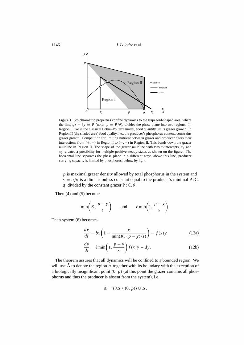
Figure 1. Stoichiometric properties confine dynamics to the trapezoid-shaped area, wherethe line,qx + θy = P (note: p = P/θ ), divides the phase plane into two regions. InRegion I, like in the classical Lotka–Volterra model, food quantity limits grazer growth. InRegion II (the shaded area) food quality, i.e., the producer’s phosphorus content, constrainsgrazer growth. Competition for limiting nutrient between grazer and producer alters theirinteractions from(+,−) in Region I to(−,−) in Region II. This bends down the grazernullcline in Region II. The shape of the grazer nullcline with twox-intercepts,x1 andx2, creates a possibility for multiple positive steady states as shown on the figure. Thehorizontal line separates the phase plane in a different way: above this line, producercarrying capacity is limited by phosphorus; below, by light.

p is maximal grazer density allowed by total phosphorus in the system ands = q/θ is a dimensionless constant equal to the producer’s minimal P:C,q, divided by the constant grazer P:C, θ .

Then (4) and (5) become

min

(K ,

p− y

s

)and emin

(1,

p− y

x

).

Then system (6) becomes

dx

dt= bx

(1−

x

min(K , (p− y)/s)

)− f (x)y (12a)

dy

dt= emin

(1,

p− y

x

)f (x)y− dy. (12b)

The theorem assures that all dynamics will be confined to a bounded region. Wewill use 1 to denote the region1 together with its boundary with the exception ofa biologically insignificant point(0, p) (at this point the grazer contains all phos-phorus and thus the producer is absent from the system), i.e.,

1 = (∂1 \ (0, p)) ∪1.


Note, that initial conditions outside of1 are meaningless, because they wouldmean that we start with higher phosphorus concentration in the system than thedefined total concentration ofP.

3.2. Nullclines. To simplify the analysis, we rewrite system (12) in the follow-ing form:

x′ = x F(x, y) (13a)

y′ = yG(x, y), (13b)

where

F(x, y) = b

(1−

x

min(K , (p− y)/s)

)−

f (x)

xy (14a)

G(x, y) = emin

(1,

p− y

x

)f (x)− d = emin

(f (x), (p− y)

f (x)

x

)− d.

(14b)

Conditions (9) assure that system (13) is well defined and partial derivatives ofF andG exist almost everywhere on1:

Fx =∂F

∂x=

b

min(K , (p− y)/s)−

(f (x)

x

)′y (15)

Fy =∂F

∂y=

{−

f (x)x < 0 if y < p− sK

−(bsx)/(p− y)2− f (x)x < 0 if y > p− sK

(16)

Gx =∂G

∂x=

{e f ′(x) > 0 if y < p− x

e(p− y)( f (x)

x

)′< 0 if y > p− x

(17)

Gy =∂G

∂y=

{0 if y < p− x

−e f (x)x < 0 if y > p− x.

(18)

A very important feature of the model is the change in the sign ofGx, whichmeasures the effect of producer density on grazer net growth rate. Conventionalecological theory considers this effect as positive (or 0 in the case of the saturationof grazer response) and thus traditionally classifies grazer–producer and indeedall other predator–prey interactions as (+,−). However, in this model the line,y = p− x, divides the phase plane into two regions (see Fig.1):

(i) Region I, y < p − x, where only food quantity (energy or carbon) limitsgrazer growth, (+,−), and


(ii) Region II, y > p − x, where food quality (phosphorus content) constrainsgrazer growth, (−,−).

Hence, in Region I the grazer growth benefits from higher prey densities like inclassical predator–prey theory. However, in Region II the grazer indirectly com-petes with its prey for phosphorus. Such competition shifts the grazer–producerrelationship from a conventional (+,−) in Region I to an unusual (−,−) in Re-gion II. This shift is responsible for the peculiar shape of the grazer nullcline, whichin most predator–prey models is a non-decreasing line. Before we consider itsshape in model (6), let us state our last assumption, without which the grazer willnot have a chance to persist.

ASSUMPTION 4. The maximal net growth rate of the grazer is positive.

Mathematically, this is equivalent to the following inequality

max1

G(x, y) > 0. (19)

The grazer nullcline is determined by

G(x, y) = 0. (20)

From continuity ofG(x, y), (19) andG(0,0) < 0 it follows that (20) has a solu-tion. Hence, the grazer nullcline exists in1 and its slope is given by

−Gx/Gy. (21)

Using (17), (18) and (21) we find that in Region I, the grazer nullcline is a verticalsegment (undefined slope) like in the Rosenzweig–MacArthur model, while in Re-gion II it is declining. The declining grazer nullcline reflects the negative effect ofdiminishing food quality at higher producer density. Next, we show that the grazernullcline has exactly twox-intercepts, which are solutions of

g(x) ≡ G(x,0) = 0. (22)

Sinceg′(x) = Gx(x,0), (17) yields thatg(x) is strictly increasing for 0≤ x < pand strictly decreasing forp ≤ x. Hence, maxx≥0 g(x) = g(p). Observe thaton 1,

G(x,0) ≥ G(x, y). (23)

Using (23) and (19), we find that

g(p) = maxx≥0

g(x) = maxx≥0

G(x,0) ≥ max1

G(x, y) > 0. (24)


Thusg(x) is a continuous function that is strictly increasing on the interval(0, p)while being negative on its left end (g(0) < 0) and positive on its right end(g(p) > 0). Thus, on this interval (22) has a unique solution, which we denotex1 (see Fig.1). The boundedness off (x) yields thatg(x) < 0 for large enoughx, and by similar arguments we find that (22) has a unique solution on(p,∞),which we denotex2. Thus, 0< x1 < p < x2. In other words, the grazer nullclinehas onex-intercept in Region I and a second one in Region II.Andersen (1997),andSchwinning and Parson (1996) analysing their higher dimensional models ob-tained hump-shaped nullclines by projecting manifolds on a plane. Interestingly,Schwinning and Parson (1996) reported the change in the type of grass–legumeinteractions from(+,−) to (−,−) due to a shift in the relative importance of ni-trogen limitation to a light limitation. Here, the triangle-shaped grazer nullclinereflects the negative role of worsening food quality on the grazer in Region II.

The producer nullcline is a solution ofF(x, y) = 0. This yields a continuouscurve withy-intercept at(0, b/ f ′(0)) andx-intercept at(k,0).

3.3. Equilibria on the boundary. To find equilibria we solve

x F(x, y) = 0 (25a)

yG(x, y) = 0. (25b)

The only boundary equilibria areE0 = (0,0) andE1 = (k,0).To determine the local stability of these equilibria, we consider the Jacobian of

system (13): (F(x, y)+ x Fx(x, y) x Fy(x, y)

yGx(x, y) G(x, y)+ yGy(x, y)

). (26)

At the origin it takes the form

J(E0) =

(b 00 −d

).

Since the determinant is negative, the eigenvalues have different signs. Thus, theorigin is always unstable in the form of a saddle.

At E1 the Jacobian is

J(E1) =

(−b Fy(k,0)0 G(k,0)

).

If G(k,0) is positive, then the determinant is negative, yielding thatE1 is un-stable. This means that the grazer can invade the system around this equilibriumpoint. Otherwise,E1 is locally asymptotically stable. The following propositionprovides a graphical criterion for the stability ofE1.


PROPOSITION 3. The steady state E1 is a saddle if it lies between the two x-intercepts of the grazer nullcline, i.e., if x1 < k < x2. If k /∈ [x1, x2], then E1 islocally asymptotically stable.

Proof. Recall thatG(k,0) = g(x) andg(x1) = g(x2) = 0. Hence,g(k) > 0 forx1 < k < x2, which meansG(k,0) > 0 holds, and henceE1 is a saddle. Ifk < x1

or k > x2, theng(k) < 0, makingE1 locally asymptotically stable. 2

3.4. Internal equilibria. Next we derive a simple graphical test that will deter-mine the local stability of any internal equilibrium of our system. Equilibria arethe intersection points of the producer and the grazer nullclines. Note that theslope of the producer and grazer nullclines at(x, y) are defined by−(Fx/Fy) and−(Gx/Gy), respectively. The hump-shaped grazer nullcline creates a possibilityfor multiple positive equilibria as Fig.1 shows. Suppose that(x∗, y∗) is one suchequilibria, i.e.,F(x∗, y∗) = 0 andG(x∗, y∗) = 0.

The Jacobian (26) at (x∗, y∗) takes the following form:

J(x∗, y∗) =

(x∗Fx(x∗, y∗) x∗Fy(x∗, y∗)y∗Gx(x∗, y∗) y∗Gy(x∗, y∗)

).

Its determinant and trace are

Det(J(x∗, y∗))= x∗y∗(FxGy − FyGx) (27)

Tr(J(x∗, y∗))= x∗Fx + y∗Gy. (28)

We split the analysis into two cases depending on whether the equilibrium(x∗, y∗)is in Region I or II:

(i) Suppose,(x∗, y∗) lies in Region I (y∗ < p− x∗). Then (16)–(18) yield thatat (x∗, y∗), Fy < 0, Gx > 0, Gy = 0. Therefore, the sign of (27) is positive,while

sign(Tr(J(x∗, y∗))) = sign(Fx) = sign

(−

Fx

Fy

).

Since the fraction−(Fx/Fy) is the slope of the producer nullcline it followsthat (x∗, y∗) is locally asymptotically stable if the producer nullcline is de-clining at (x∗, y∗). If it is increasing at(x∗, y∗), then the equilibrium is arepeller.

(ii) Suppose,y∗ > p − x∗. Then (16)–(18) yield that at(x∗, y∗), Fy < 0,Gx < 0, Gy < 0. An elementary derivation shows that

sign(Det(J)) = sign(FxGy − FyGx) = sign

(FxGy − FyGx

FyGy

)= sign

(−

Gx

Gy−

(−

Fx

Fy

)).


Hence, if the slope of the producer nullcline at(x∗, y∗) is greater then the grazer’s,then the determinant (27) is negative, yielding(x∗, y∗) as a saddle. If the grazernullcline has larger slope, then the determinant is positive which makes the eigen-values of the same sign as the trace (28). Recalling thatGx andGy are negative,we find that

0> −Gx

Gy> −

Fx

Fy. (29)

Condition (29) together withFy < 0 yields thatFx < 0. Therefore, the trace (28)is negative, so(x∗, y∗) is locally asymptotically stable if the grazer nullcline haslarger slope than the producer’s.

We summarize the conditions for the stability of all possible equilibria (with theexception of non-generic cases, such as touching nullclines or 0 eigenvalues; whichare biologically insignificant) in the following theorem. The acronym LAS standsfor locally asymptotically stable.

THEOREM 4. Boundary equilibria: The origin is a saddle. The only other equi-librium on the boundary is E1 = (k,0). It is a saddle if it lies between the twox-intercepts of the grazer nullcline, i.e., if x1 < k < x2. If it lies outside of[x1, x2],then E1 is LAS.

Internal equilibria: In Region I the internal equilibrium is LAS if the producernullcline at it is decreasing; if the producer nullcline at it is increasing, then theequilibrium is a repeller. In Region II any internal equilibrium is LAS if the pro-ducer nullcline at it declines steeper then the grazer’s; otherwise, the equilibriumis a saddle.

4. NUMERICAL EXPERIMENTS

In this section we provide results of numerical experiments that are in somesense analogous to previously considered laboratory experiments investigating sto-ichiometric aspects of phytoplankton–zooplankton interactions (Urabe and Sterner,1996; Sterneret al., 1998). We choose the functional response as a Monod typefunction, i.e.,

f (x) =cx

a+ x. (30)

The parameter values are listed in the Table1, where we usedAndersen (1997),andUrabe and Sterner (1996) for guidance in setting parameters at biologicallyrealistic values. We used XPP software developed by Bard Ermentrout (http://www.pitt.edu/~phase) for the numerical runs and as an aid in obtaining allfigures.

http://www.pitt.edu/~phase

http://www.pitt.edu/~phase


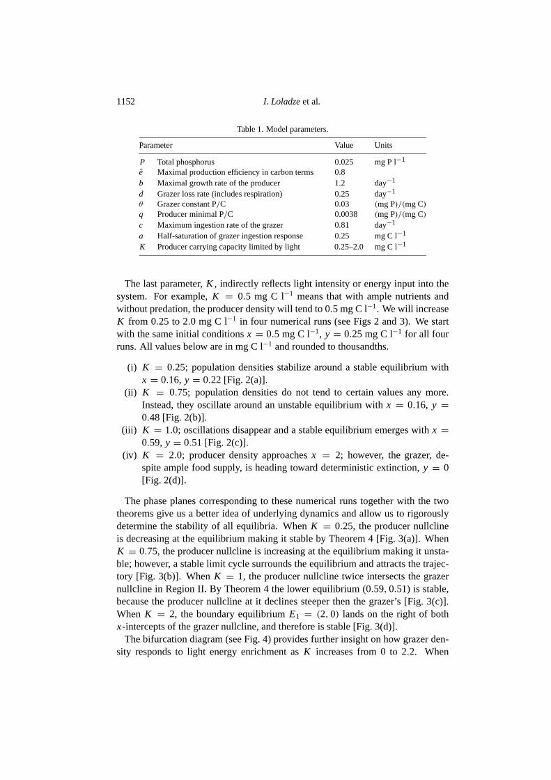
Table 1. Model parameters.

Parameter Value Units

P Total phosphorus 0.025 mg P l−1

e Maximal production efficiency in carbon terms 0.8b Maximal growth rate of the producer 1.2 day−1

d Grazer loss rate (includes respiration) 0.25 day−1

θ Grazer constant P/C 0.03 (mg P)/(mg C)q Producer minimal P/C 0.0038 (mg P)/(mg C)c Maximum ingestion rate of the grazer 0.81 day−1

a Half-saturation of grazer ingestion response 0.25 mg C l−1

K Producer carrying capacity limited by light 0.25–2.0 mg C l−1

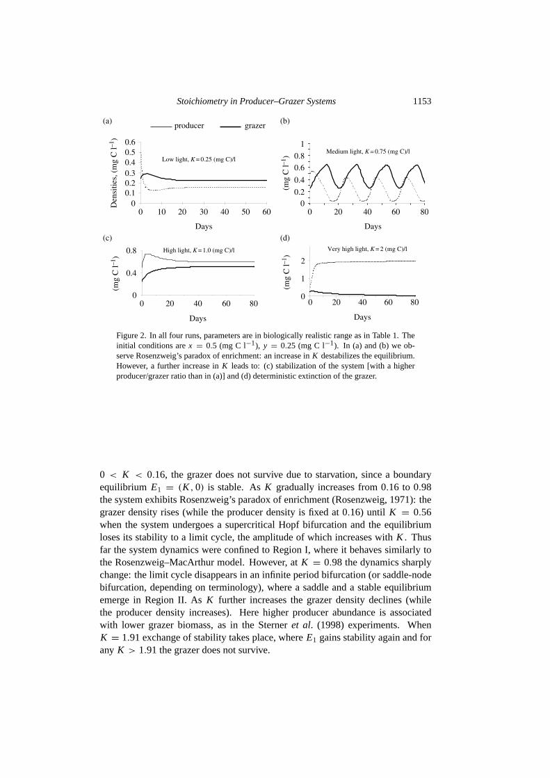
The last parameter,K , indirectly reflects light intensity or energy input into thesystem. For example,K = 0.5 mg C l−1 means that with ample nutrients andwithout predation, the producer density will tend to 0.5 mg C l−1. We will increaseK from 0.25 to 2.0 mg C l−1 in four numerical runs (see Figs2 and3). We startwith the same initial conditionsx = 0.5 mg C l−1, y = 0.25 mg C l−1 for all fourruns. All values below are in mg C l−1 and rounded to thousandths.

(i) K = 0.25; population densities stabilize around a stable equilibrium withx = 0.16, y = 0.22 [Fig. 2(a)].

(ii) K = 0.75; population densities do not tend to certain values any more.Instead, they oscillate around an unstable equilibrium withx = 0.16, y =0.48 [Fig. 2(b)].

(iii) K = 1.0; oscillations disappear and a stable equilibrium emerges withx =0.59, y = 0.51 [Fig. 2(c)].

(iv) K = 2.0; producer density approachesx = 2; however, the grazer, de-spite ample food supply, is heading toward deterministic extinction,y = 0[Fig. 2(d)].

The phase planes corresponding to these numerical runs together with the twotheorems give us a better idea of underlying dynamics and allow us to rigorouslydetermine the stability of all equilibria. WhenK = 0.25, the producer nullclineis decreasing at the equilibrium making it stable by Theorem 4 [Fig.3(a)]. WhenK = 0.75, the producer nullcline is increasing at the equilibrium making it unsta-ble; however, a stable limit cycle surrounds the equilibrium and attracts the trajec-tory [Fig. 3(b)]. WhenK = 1, the producer nullcline twice intersects the grazernullcline in Region II. By Theorem 4 the lower equilibrium (0.59,0.51) is stable,because the producer nullcline at it declines steeper then the grazer’s [Fig.3(c)].When K = 2, the boundary equilibriumE1 = (2,0) lands on the right of bothx-intercepts of the grazer nullcline, and therefore is stable [Fig.3(d)].

The bifurcation diagram (see Fig.4) provides further insight on how grazer den-sity responds to light energy enrichment asK increases from 0 to 2.2. When


0

(a) (b)

(c) (d)

00

0.4

(mg

C l–1

)

0.8

20 40

Days

60 80

00.10.20.3

Den

sitie

s, (

mg

C l–1

)

0.40.50.6

10 20

Low light, K = 0.25 (mg C)/l

High light, K = 1.0 (mg C)/l

0 20 40 60 800

1(m

g C

l–1)

2

Days

Very high light, K = 2 (mg C)/l

producer grazer

30

Days

40 50 60 0 20 40 60 800

0.2

0.4

0.6

0.8

1

(mg

C l–1

)

Medium light, K = 0.75 (mg C)/l

Days

Figure 2. In all four runs, parameters are in biologically realistic range as in Table1. Theinitial conditions arex = 0.5 (mg C l−1), y = 0.25 (mg C l−1). In (a) and (b) we ob-serve Rosenzweig’s paradox of enrichment: an increase inK destabilizes the equilibrium.However, a further increase inK leads to: (c) stabilization of the system [with a higherproducer/grazer ratio than in (a)] and (d) deterministic extinction of the grazer.

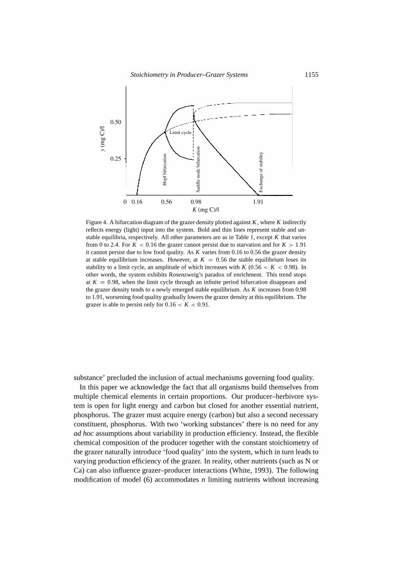
0 < K < 0.16, the grazer does not survive due to starvation, since a boundaryequilibrium E1 = (K ,0) is stable. AsK gradually increases from 0.16 to 0.98the system exhibits Rosenzweig’s paradox of enrichment (Rosenzweig, 1971): thegrazer density rises (while the producer density is fixed at 0.16) until K = 0.56when the system undergoes a supercritical Hopf bifurcation and the equilibriumloses its stability to a limit cycle, the amplitude of which increases withK . Thusfar the system dynamics were confined to Region I, where it behaves similarly tothe Rosenzweig–MacArthur model. However, atK = 0.98 the dynamics sharplychange: the limit cycle disappears in an infinite period bifurcation (or saddle-nodebifurcation, depending on terminology), where a saddle and a stable equilibriumemerge in Region II. AsK further increases the grazer density declines (whilethe producer density increases). Here higher producer abundance is associatedwith lower grazer biomass, as in theSterneret al. (1998) experiments. WhenK = 1.91 exchange of stability takes place, whereE1 gains stability again and forany K > 1.91 the grazer does not survive.


‘

y

x0 K

y

0 K 0 K

y

IIII

II

II

I

(b)

(c) (d)

‘

y

x0 K

I

(a)

x x

Figure 3. These four phase planes correspond to the four numerical runs in Fig.2.The stability type of all equlibria easily follow from the second theorem. In (a)and (b) the dynamics is confined to Region I, where the model behaves similarly to theRosenzweig–MacArthur model. In (c) and (d) the system dynamics enters Region II,where a stable equilibrium emerges. Note that, in (c) higher values ofK would corre-spond to lower grazer density and higher producer abundance. This trend continues untilthe predator cannot survive in (d).

5. DISCUSSION

Many population dynamics models, like classical models (1a), (1b) and (2a),(2b), assume that organisms and their food are made of a single constituent thatis the equivalent of energy. Such an assumption is supported by the concept ofenergy flow that views trophic levels as homogeneous substances for energy stor-age and transformation. This powerful simplification of reality is very convenientand has proven to be useful, however some of its drawbacks are not always real-ized. For example, this assumption yields that organisms should assimilate foodwith constant efficiency, because food made of a single substance cannot changeits quality. Although our everyday experience suggests that even quality of ourown food varies widely, constant production efficiencies have been a standard as-sumption in population dynamics theory. These constants are usually scaled awayduring analysis, which eliminates any clues on their effects on population dynam-ics. Nevertheless, several researchers [e.g.,Edelstein-Keshet and Rausher (1989),Koppel et al. (1996) andHuxel (1999)] considered plant–herbivore models withvariable food quality. However, the reliance of these models on a single ‘working


0.160

0.25

0.50

0.98 1.91K (mg C)/l

y (m

g C

)/l

0.56

Limit cycle

Hop

f bi

furc

atio

n

Sadd

le-n

ode

bifu

rcat

ion

Exc

hang

e of

sta

bilit

y

Figure 4. A bifurcation diagram of the grazer density plotted againstK , whereK indirectlyreflects energy (light) input into the system. Bold and thin lines represent stable and un-stable equilibria, respectively. All other parameters are as in Table1, exceptK that variesfrom 0 to 2.4. ForK < 0.16 the grazer cannot persist due to starvation and forK > 1.91it cannot persist due to low food quality. AsK varies from 0.16 to 0.56 the grazer densityat stable equilibrium increases. However, atK = 0.56 the stable equilibrium loses itsstability to a limit cycle, an amplitude of which increases withK (0.56< K < 0.98). Inother words, the system exhibits Rosenzweig’s paradox of enrichment. This trend stopsat K = 0.98, when the limit cycle through an infinite period bifurcation disappears andthe grazer density tends to a newly emerged stable equilibrium. AsK increases from 0.98to 1.91, worsening food quality gradually lowers the grazer density at this equilibrium. Thegrazer is able to persist only for 0.16< K < 0.91.

substance’ precluded the inclusion of actual mechanisms governing food quality.In this paper we acknowledge the fact that all organisms build themselves from

multiple chemical elements in certain proportions. Our producer–herbivore sys-tem is open for light energy and carbon but closed for another essential nutrient,phosphorus. The grazer must acquire energy (carbon) but also a second necessaryconstituent, phosphorus. With two ‘working substances’ there is no need for anyad hocassumptions about variability in production efficiency. Instead, the flexiblechemical composition of the producer together with the constant stoichiometry ofthe grazer naturally introduce ‘food quality’ into the system, which in turn leads tovarying production efficiency of the grazer. In reality, other nutrients (such as N orCa) can also influence grazer–producer interactions (White, 1993). The followingmodification of model (6) accommodatesn limiting nutrients without increasing


the dimension of the system:

x′ = bx

[1−

x

min(K , (N1− θ1y)/q1, . . . , (Nn − θny)/qn)

]− f (x)y

y′ = emin

(1,(N1− θ1y)/x

θ1, . . . ,

(Nn − θny)/x

θn

)f (x)y− dy,

where

Ni is the total amount of thei th nutrient in the system,qi is the producer’s minimali th nutrient content,θi is the grazer’s constant (homeostatic)i th nutrient content and all other pa-

rameters are as in system (6).

The limitation of the above model as well as models (6a) and (6b) is the ab-sence of a free nutrient pool and lack of delay in nutrient recycling as assumed inAssumption3. In nutrient-limited pelagic systems the concentration of free phos-phorus is very low or below detection. Such a low concentration should not beignored if one wishes to model competition among multiple producers. Since wemodel only one producer species, we can assume that it simply absorbs all poten-tially available phosphorus. However for terrestrial systems, even with a singleproducer, soil compartments and delays in nutrient release are of major importance(Agren and Bosatta, 1996) and addition of a free nutrient pool appears to be nec-essary. Another limitation is that models (6a) and (6b) are homogeneous in allaspects except of chemical composition of organisms. However, such ‘chemicalheterogeneity’ profoundly effects producer–grazer interactions.

• The demand of both populations for limiting phosphorus naturally boundsthe densities of both populations, even when light energy input into the sys-tem is unlimited (see Fig.1).• The carrying capacity of the producer, instead of being a static and external

factor, becomes a multivariable function that depends on energy (light) input,nutrient concentration and grazer density [see Eqns (4) and (5)].• In the system where every organism competes with every other organism for

the limiting nutrient, competition effects superimpose on predator–prey in-teractions. This divides the grazer–producer phase plane into two regions.In Region I energy (carbon) availability regulates grazer growth and grazer–producer interactions are the traditional(+,−) type. However, in Region IIfood quality (phosphorus content) controls grazer growth and changes grazer–producer relationships to a competitor type (−,−). This creates a possibilityfor multiple positive equilibria and deterministic extinction of the grazer (seeFig. 1).• The system exhibits a paradox ofenergy enrichment. Intense energy (light)

enrichment substantially elevates producer density, however, despite such anabundant food supply the grazer decreases its growth rate and drives itself todeterministic extinction [see Figs2(d), 3(d) and4].


From an energetics point of view the paradox of energy enrichment is a trueparadox: higher energy (food) consumption should not decrease growth rate. How-ever, it is easily solved by ‘food quality’ arguments, as higher producer densitiescorrespond to its lower phosphorus content and thus, lower production efficien-cies for the grazer. Hence, in estimating effects of enrichment on producer–grazerand longer food chains one should take into account both food quantity and foodquality. For example, carbon dioxide enrichment may affect herbivores throughchanges in producer abundance but also in its stoichiometry. Since both light andnutrients can affect quality as well as quantity, a question arises: how does energyenrichment (that leads here to carbon enrichment of the producer) differ from nutri-ent enrichment? Motivated by this question we constructed a bifurcation diagram(Fig. 5), where different dynamical outcomes were presented on theK–P plane(K is associated with light intensity andP is total phosphorus in the system). Wefind a striking difference between light and phosphorus enrichment. Light energyenrichment (horizontal arrow) may destabilize as well as stabilize the system, butultimately leads to the deterministic extinction of the grazer. In contrast, phospho-rus enrichment (vertical arrow) can only destabilize the system; however, it doesnot lead to the extinction of the grazer. Rosenzweig’s paradox of enrichment (usu-ally viewed as destabilization of predator–prey interactions through Hopf bifurca-tion) holds only in a limited light–phosphorus range. Yet, under wider definition assystem destabilization or grazer’s extinction, the paradox of enrichment holds in arather wideK–P range.

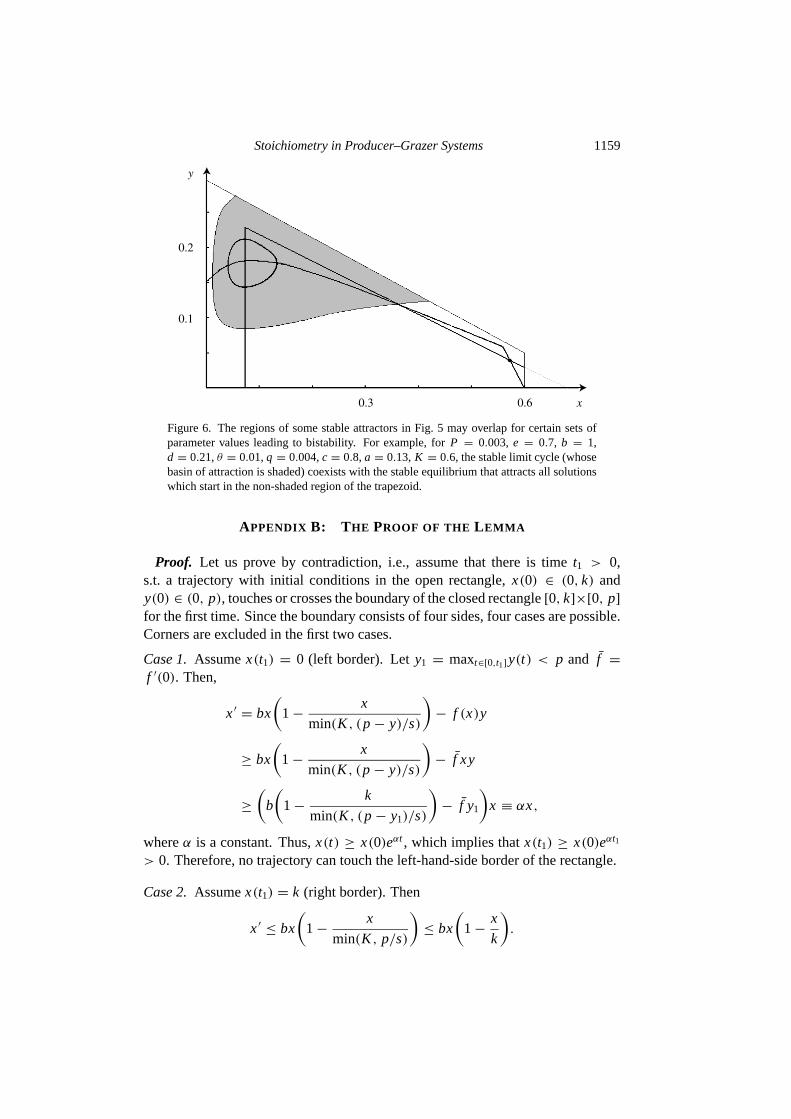
In Fig.5 the various regions of stable attractors do not overlap, meaning that onlyone stable attractor exists for any particular (K , P) pair and other parameters arefixed as in Table1. However, bistability may arise for certain sets of parametervalues that deviate from the ones in Table1 but are still in a biologically realisticrange. For example, in Fig.6, depending on initial conditions, the system can beattracted to a stable limit cycle or a stable equilibrium. This suggests that in suchsystems an externally caused shift in population density may significantly changesystem behavior and producer/grazer ratio.

The introduction of stoichiometric reality into population dynamics theory raisesother questions. How will space, age, or size-structured models be affected by sto-ichiometric considerations? When a stoichiometric perspective is brought to bearon all interactions, how will the community matrix of an ecosystem changes? Willcompetitive and mutualistic interactions always be a (−,−) or (+,+) type, respec-tively? Will the competitive exclusion principle still hold in a model that is chem-ically heterogeneous but homogeneous in all other aspects? The analysis of themodel shows that stoichiometry may dampen potentially destructive oscillationsby reducing energy flow to the grazer (see Fig. 2(b), 2(c) and Fig. 4). Here, a cer-tain degree of weakening of predator-prey interactions contributes to the stabilityof the system. This supports the McCann (2000) statement that “weak interactionsserve to limit energy flow in a potentially strong consumer-resource interactionsand, therefore, to inhibit runaway consumption that destabilizes the dynamics of


1

Grazer extinction due to low food quality

Paradox of energy enrichment

Stable equilibrium

in Region II

Limit cycle

Rosenzweig's paradox of enrichment

Gra

zer

extin

ctio

n du

e to

low

foo

d ab

unda

nce

Stab

le e

quili

briu

min

Reg

ion

I

Nut

rien

t enr

ichm

ent

1

0.5

2 (mg C)/l

(mg

P)/l

P

K

Figure 5. The regions of existence of all stable attractors are drawn on theK–P plane withall other parameters fixed as in Table1. Energy enrichment of the system (the long hor-izontal arrow) leads the grazer through (steady state)/(cycle)/(steady state)/(deterministicextinction). It drastically differs from nutrient enrichment (the vertical arrow) that maydestabilize the system; however, it does not lead to grazer extinction. Rozensweig’s para-dox of enrichment holds in a limited range of light/nutrient parameters, where the systemundergoes Hopf bifurcation. Note, that balanced light/nutrient enrichment, (e.g., along theshaded area of the stable equilibrium in Region II) may leave the system dynamics quali-tatively unchanged. Hence, the effects of enrichment strongly depend on its type: energy,nutrient or combined energy/nutrient enrichment.

food webs”. The question arises as to how stoichiometry contributes to the diver-sity and stability of an ecosystem.

ACKNOWLEDGEMENTS

The authors express their gratitude to T. Andersen for insightful discussions. Weare grateful to W. F. Fagan, S. G. Fisher, H. Thieme and two anonymous refereesfor valuable comments and suggestions on an earlier version of this paper. Thiswork was supported by National Science Foundation grant DEB-9725867.

APPENDIX A: T HE PROPERTIES OF THE FUNCTIONAL RESPONSE, f (x)f (x)f (x)

We have that( f (x)/x)′ = (x f ′(x)− f (x))/x2. Let l (x) ≡ x f ′(x)− f (x). Thenby (3), l (0) = 0 andl ′(x) = x f ′′(x) < 0. Hence,( f (x)/x)′ < 0 for x > 0. Bydefinition of a limit and sincef (0) = 0, it follows that limx→0( f (x)/x) = f ′(0).


0.3

0.1

0.2

y

0.6 x

Figure 6. The regions of some stable attractors in Fig.5 may overlap for certain sets ofparameter values leading to bistability. For example, forP = 0.003, e = 0.7, b = 1,d = 0.21,θ = 0.01,q = 0.004,c = 0.8, a = 0.13, K = 0.6, the stable limit cycle (whosebasin of attraction is shaded) coexists with the stable equilibrium that attracts all solutionswhich start in the non-shaded region of the trapezoid.

APPENDIX B: T HE PROOF OF THE L EMMA

Proof. Let us prove by contradiction, i.e., assume that there is timet1 > 0,s.t. a trajectory with initial conditions in the open rectangle,x(0) ∈ (0, k) andy(0) ∈ (0, p), touches or crosses the boundary of the closed rectangle[0, k]×[0, p]for the first time. Since the boundary consists of four sides, four cases are possible.Corners are excluded in the first two cases.

Case 1.Assumex(t1) = 0 (left border). Lety1 = maxt∈[0,t1]y(t) < p and f =f ′(0). Then,

x′ = bx

(1−

x

min(K , (p− y)/s)

)− f (x)y

≥ bx

(1−

x

min(K , (p− y)/s)

)− f xy

≥

(b

(1−

k

min(K , (p− y1)/s)

)− f y1

)x ≡ αx,

whereα is a constant. Thus,x(t) ≥ x(0)eαt , which implies thatx(t1) ≥ x(0)eαt1

> 0. Therefore, no trajectory can touch the left-hand-side border of the rectangle.

Case 2.Assumex(t1) = k (right border). Then

x′ ≤ bx

(1−

x

min(K , p/s)

)≤ bx

(1−

x

k

).


The standard comparison argument yields thatx(t) < k for all t ∈ [0, t1] and thus,no trajectory touches the right-hand-side border.

Case 3.Assume nowy(t1) = 0 (bottom border). Then,y′ = emin(1, (p −y)/x) f (x)y − dy ≥ −dy. Hence,y(t) ≥ y(0)e−dt > 0. This excludes thepossibility that a trajectory touches corners(0,0) and(k,0) as well.

Case 4.Assumey(t1) = p (top border). Then

y′ ≤ ep− y

xf (x)y ≤ e(p− y) f ′(0)y = e f ′(0)py

(1−

y

p

).

Using the standard comparison argument we find thaty(t) < p for all t ∈ [0, t1].This case takes care of the remaining two corners(0, p) and(k, p). 2

APPENDIX C: T HE PROOF OF THE BOUNDEDNESS AND I NVARIANCE

THEOREM

Proof. Lemma1 assures that trajectories will satisfy the first two inequalitiesin (11). Suppose that the last inequality in (11) is not true. Then lett1 > 0 be thefirst time it is violated, i.e.,

sx(t1)+ y(t1) = p. (C1)

Since for allt ∈ [0, t1), sx(t)+ y(t) < p, it follows that

sx′(t1)+ y′(t1) ≥ 0. (C2)

From (C1) it follows thatx(t1) = (p− y(t1))/s, which we substitute in (12(a)) toobtain bounds onx′(t1):

x′(t1) = bx(t1)

(1−

x(t1)

min(K , (p− y(t1))/s)

)− f (x(t1))y(t1) (C3)

≤ bx(t1)

(1−

x(t1)

(p− y(t1))/s

)− f (x(t1))y(t1) = − f (x(t1))y(t1).

From (C1) it follows thats = (p− y(t1))/x(t1), which we substitute in (12(b)) toobtain bounds ony′(t1):

y′(t1) = emin{1, (p− y(t1))/x(t1)} f (x(t1))y(t1)− dy(t1) (C4)

≤ ep− y(t1)

x(t1)f (x(t1))y(t1) = es f(x(t1))y(t1).


Using (C3), (C4) and the fact thate< 1, we obtain the following:

sx′(t1)+ y′(t1) ≤ −s f(x(t1))y(t1)+ es f(x(t1))y(t1)

= s f(x(t1))y(t1)(−1+ e) < 0.

This contradicts (C2) and completes the proof. 2

REFERENCES

Agren, G. and E. Bosatta (1996).Theoretical Ecosystem Ecology: Understanding ElementCycles, NY: Cambridge University Press.

Andersen, T. (1997).Pelagic Nutrient Cycles: Herbivores as Sources and Sinks, NY:Springer-Verlag.

Andersen, T. and D. O. Hessen (1991). Carbon, nitrogen, and phosphorus content of fresh-water zooplankton.Limnol. Oceanogr.36, 807–814.

DeMott, W. R. (1998). Utilization of cyanobacterium and phosphorus-deficient green algaeas a complementary resource by daphnids.Ecology79, 2463–2481.

Droop, M. R. (1974). The nutrient status of algal cells in continuous culture.J. Mar. Biol.Assoc. UK55, 825–855.

Edelstein-Keshet, L. and M. D. Rausher (1989). The effects of inducible plant defenses onherbivore populations.Am. Nat.133, 787–810.

Elser, J. J., T. H. Chrzanowski, R. W. Sterner and K. H. Mills (1998). Stoichiometricconstraints on food web dynamics: a whole-lake experiment on the Canadian shield.Ecosystems1, 120–136.

Elser, J. J., E. R. Marzolf and C. R. Goldman (1990).Can. J. Fisheries Aquatic Sci.47,1468–1477.

Elser, J. J. and J. Urabe (1999). The stoichiometry of consumer-driven nutrient recycling:theory, observations, and consequences.Ecology80, 735–751.

Hagen, J. B. (1992).An Entangled Bank: The Origins of Ecosystem Ecology, NewBrunswick, NJ: Rutgers.

Hessen, D. O. and T. Andersen (1992). The algae–grazer interface: feedback mechanismlinked to elemental ratios and nutrient cycling.Archiv Fuer Hydrobiologie Ergebnisseder Limnologie35, 111–120.

Huxel, G. R. (1999). On the influence of food quality in consumer–resource interactions.Ecology Lett.2, 256–261.

Kooijman, S. A. L. M. (2000).Dynamic energy and mass budgets in biological systems,Cambridge, U.K: Cambridge University Press.

Koppel, J., J. Huisman, R. Wal and H. Olff (1996). Patterns of herbivory along productivitygradient: and empirical and theoretical investigation.Ecology77, 736–745.

Lindeman, R. L. (1942). The trophic-dynamic aspect of ecology.Ecology23, 399–418.Lotka, A. J. (1925).Elements of Physical Biology, Baltimore: Williams and Wilkins.

Reprinted asElements of Mathematical Biology(1956) New York: Dover.


McCann, K. S. (2000). The diversity-stability debate.Nature405, 228–233.Odum, E. P. (1959).Fundamentals of Ecology, Philadelphia: W.B. Saunders.Odum, E. P. (1968). Energy flow in ecosystems: a historical view.Am. Zoologist8, 11–18.Odum, H. P. (1957). Trophic structure and productivity of Silver Springs.Ecol. Mono-

graphs27, 55–112.Odum, H. P. (1960). Ecological potential and analogue circuits for the ecosystem.Am.

Scientist48, 1–8.Reiners, W. A. (1986). Complementary models for ecosystems.Am. Nat.127, 59–73.Rosenzweig, M. L. (1971). Paradox of enrichment: destabilization of exploitation ecosys-

tems in ecological time.Science171, 385–387.Schindler, D. W. (1977). Evolution of phosphorus limitation in lakes.Science195, 260–

262.Schwinning, S. and A. J. Parsons (1996). Analysis of the coexistence mechanisms for

grasses and legumes in grazing systems.J. Ecology84, 799–813.Sterner, R. W. (1990). The ratio of nitrogen to phosphorus resupplied by herbivores: zoo-

plankton and the algal competitive arena.Am. Nat.136, 209–229.Sterner, R. W., J. Clasen, W. Lampert and T. Weisse (1998). Carbon : phosphorus stoi-

chiometry and food chain production.Ecology Lett.1, 146–150.Sterner, R. W. and D. O. Hessen (1994). Algal nutrient limitation and the nutrient of aquatic

herbivores.Ann. Rev. Ecol. Syst.25, 1–29.Tilman, D. (1982).Resource Competition and Community Structure, Princeton, NJ: Prince-

ton University Press.Urabe, J. and R. W. Sterner (1996). Regulation of herbivore growth by the balance of

light and nutrients.Proc. Natl. Acad. Sci. USA93, 8465–8469.White, T. C. R. (1993).The Inadequate Environment: Nitrogen and the Abundance of

Animals, NY: Springer-Verlag.

Received 20 March 2000 and accepted 29 June 2000

Documents

Stoichiometry in Producer-Grazer Systems: Linking Energy Flow with Element Cycling