Stock-rebuilding time isopleths and constant-F stock-rebuilding plans for overfished stocks

519

Abstract–Stock-rebuilding time isopleths relate constant levels of fishing mortality (F), stock biomass, and management goals to rebuilding times for overfished stocks. We used simulation models with uncertainty about FMSY and variability in annual intrinsic growth rates (ry) to calculate rebuilding time isopleths for Georges Bank yellowtail flounder, Limanda ferruginea, and cowcod rockfish, Sebastes levis, in the Southern California Bight. Stock-rebuilding time distributions from stochastic models were variable and rightskewed, indicating that rebuilding may take less or substantially more time than expected. The probability of long rebuilding times increased with lower biomass, higher F, uncertainty about FMSY, and autocorrelation in ry values. Uncertainty about FMSY had the greatest effect on rebuilding times. Median recovery times from simulations were insensitive to model assumptions about uncertainty and variability, suggesting that median recovery times should be considered in rebuilding plans. Isopleths calculated in previous studies by deterministic models approximate median, rather than mean, rebuilding times. Stochastic models allow managers to specify and evaluate the risk (measured as a probability) of not achieving a rebuilding goal according to schedule. Rebuilding time isopleths can be used for stocks with a range of life histories and can be based on any type of population dynamics model. They are directly applicable with constant F rebuilding plans but are also useful in other cases. We used new algorithms for simulating autocorrelated process errors from a gamma distribution and evaluated sensitivity to statistical distributions assumed for ry. Uncertainty about current biomass and fishing mortality rates can be considered with rebuilding time isopleths in evaluating and designing constant-F rebuilding plans.

Manuscript accepted 12 Febraury 2002. Fish. Bull. 100:519–536 (2002).

Stock-rebuilding time isopleths and constant-F stock-rebuilding plans for overfished stocks

Larry D. Jacobson Steven X. Cadrin Northeast Fisheries Science CenterNational Marine Fisheries Service166 Water StreetWoods Hole, MA 02543E-mail address (for L. D. Jacobson): [email protected]

Stock-rebuilding plans proposed for (Fig. 1, and Thompson, 1999) reduces overfished stocks are best evaluated by FThreshold from the FMSY level linearly to stock-specific simulation analysis (e.g. zero as biomass declines from BThreshold. PFMC1). However, general approaches In cases where BMSY and FMSY can not are also valuable because many stocks be estimated, reasonable proxy values are overfished (NMFS, 1999) and (e.g. one-half unfished biomass or F0.1) default or generic rebuilding plans can are typically used instead. be used without extensive analyses for The goal for most rebuilding plans each species (e.g. PFMC2; Applegate et under the SFA is to achieve the target al.3). In this article we show how stock- biomass level (BMSY or an acceptable rebuilding time isopleths can be used proxy level) in ten years or less. Even to design, evaluate, and monitor prog- with zero fishing mortality, ten years ress of “constant F ” and other types may not be sufficient to rebuild some of rebuilding plans. Constant-F stock- overfished stocks. In such cases, the rebuilding plans maintain fishing mor- Guidelines for National Standard 1 altality at a fixed level until the stock is low a rebuilding time period no longer rebuilt, and are relatively simple and than one mean generation time (Reeasy to analyze. The isopleth approach strepo et al., 1998) plus the expected is easy to use as both a general and time to recovery in the absence of fishstock-specific tool. ing mortality (DOC, 1998).

The U.S. Sustainable Fisheries Act (SFA) mandates rebuilding plans for overfished stocks (DOC, 1996, 1998).

1 PFMC (Pacific Fishery Management Council). 1999. The coastal pelagic species

Federally managed stocks are consid- fishery management plan, Amendment 8,ered overfished when stock biomass is 405 p. Pacific Fishery Management Counless than the biomass threshold (BThresh- cil, 7700 NE Ambassador Place, Portland,

old) defined in the Fishery Manage- OR, 97220-1384.

ment Plan (FMP). National Standard 2 PFMC (Pacific Fishery Management Council). 1999. Status of the Pacific Coast1 (DOC, 1998) for the SFA indicates groundfish fishery through 1999 and rec

that BThreshold should be the greater ommended acceptable biological catch for of one-half of BMSY (the theoretical 2000 stock assessment and fishery evaluabiomass level for maximum sustained tion, 230 p. Pacific Fishery Management

yield, MSY) or the minimum biomass Council, 7700 NE Ambassador Place, Portland, OR, 97220-1384.

from which rebuilding to BMSY could 3 Applegate, A., S. Cadrin, J. Hoenig, C.be expected to occur within ten years Moore, S. Murawski, and E. Pikitch. if the stock is exploited at FThreshold. 1998. Evaluation of existing overfishing Typically, FThreshold = FMSY (the theo- definitions and recommendations for new retical fishing mortality rate for MSY) overfishing definitions to comply with the

when current biomass is at or above Sustainable Fisheries Act, 179 p. New England Fishery Management Council,

BThreshold, and FThreshold < FMSY at lower 50 Water Street, Mill 2, Newburyport, MA biomass levels. A common approach 01950.

520 Fishery Bulletin 100(3)

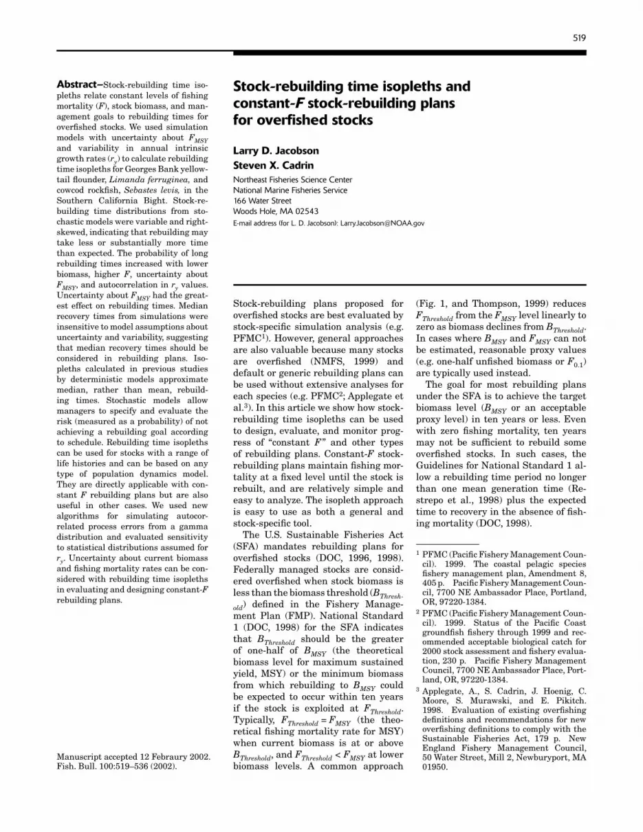
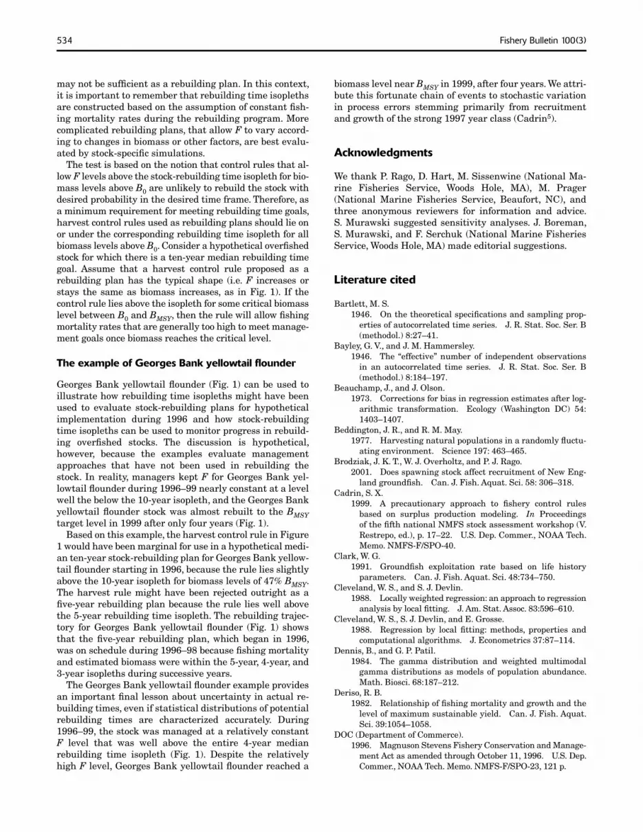
Figure 1 Isopleths for median rebuilding times based on a deterministic logistic population growth model (model type 1) for Georges Bank yellowtail flounder with FMSY=0.3. Also shown are a common harvest control rule, and the biomass-F trajectory during 1996–99 for Georges Bank yellowtail flounder. The harvest control rule specifies a maximum (threshold) F as a function of stock biomass level. The biomass-F trajectory shows a time series of F and biomass estimates from virtual population analysis (VPA, Cadrin5).

Relative biomass (B/BMSY)

0.0 0.2 0.4 0.6 0.8 1.0

Fis

hing

mor

talit

y (p

er y

ear)

0.0

0.1

0.2

0.3

10-year Isopleth 5-year Isopleth 4-year Isopleth 3-year Isopleth 2-year Isopleth Control Rule VPA

1999

Stock-rebuilding time isopleths

Cadrin (1999) calculated theoretical recovery times for Georges Bank yellowtail flounder (Limanda ferruginea) and used rebuilding time isopleths to depict trends in stock biomass in relation to fishing mortality. Calculations were based on a deterministic logistic population growth model with a range of constant annual fishing mortality rates (F̃=zero to FMSY) and a range of initial biomass levels less than the target level (B0=zero to BMSY). Recovery time was the number of years required for stock biomass to increase from an initial overfished biomass level (B0<BThreshold) to the biomass target BTarget=BMSY, assuming a constant annual fishing mortality rate. Rebuilding time isopleths were formed by connecting points of initial biomass and

˜constant fishing mortality (B0, FB0) with the same recovery

time (Fig. 1). For example, beginning at the initial biomass ˜level B0<BTarget, any constant fishing mortality rate FB0

on the 10-year isopleth would theoretically rebuild the stock to BTarget in ten years. In contrast, any constant-F value

˜ < FB0 (below or to the right of the isopleth) would rebuild

˜the stock sooner and any constant F values > FB0 (above

or to the left of the isopleth) would rebuild the stock later. Rebuilding time isopleths were used to develop overfishing definition options for nine overfished New England groundfish stocks (Applegate et al.3).

In this article, we calculate stock-rebuilding time isopleths based on stochastic population dynamics models and characterize statistical distributions (mean, median, and percentiles) of stock-rebuilding times under different assumptions about uncertainty and process error (pro

cess errors are uncertainty in population dynamics due to natural variability in growth, recruitment, and other biological factors, Hilborn and Walters, 1992). Like Cadrin (1999), we use logistic population growth models, but our analysis includes uncertainty about FMSY and autocorrelated process errors in production. We analyze rebuilding times for two stocks (cowcod rockfish, Sebastes levis, and Georges Bank yellowtail flounder) with different life histories, levels of FMSY, and autocorrelation in production process errors (the calculations are examples only and not for use by managers). We also describe how stock-rebuilding time isopleths from deterministic and stochastic models can be used to develop and evaluate rebuilding plans and to monitor their progress.

Materials and methods

Following Prager (1994), we used the continuous time version of the logistic population dynamic model in simulation calculations.4 In particular, for the logistic population growth parameter ry (subscripted to represent the value in year y) carrying capacity K, by= ry/K, and ay= ry-Fy≠0:

aya B ey y . (1)By+1 = ay + byBy (e

ay − 1)

4 SAS simulation program code available from the senior author.

Jacobson and Cadrin: Stock-rebuilding time isopleths and constant-F stock-rebuilding plans for overfished stocks 521

Table 1 Six types of simulation models used to estimate rebuilding time isopleths. Model types include all of the meaningful combinations of uncertainty about FMSY and variance and autocorrelation in production process errors.

CV for Variance Autocorrelation Model uncertainty in process in process type FMSY (%) errors (%) errors (ρ)

1 Zero 0 zero No uncertainty about FMSY; deterministic production

2 0 zero Uncertainty about FMSY; deterministic production

3 Zero from stock zero No uncertainty about FMSY; stochastic production; assessment no autocorrelation

4 20 from stock zero Uncertainty about FMSY; stochastic production; assessment no autocorrelation

5 Zero from stock from stock assessment No uncertainty about FMSY; stochastic production; assessment with autocorrelation

6 20 From stock from stock assessment Uncertainty about FMSy; stochastic production; assessment with autocorrelation

in Description

20

When fishing and the intrinsic rate of increase exactly balance (ay= ry–Fy=0):

B By+1 = y . (2)

1 + b By y

Note that biomass declines (By+1<By) when ry–Fy= 0 because ry is a maximum value defined in the limit as biomass approaches zero (Eq. 1).

Following Beddington and May (1977) and May et al. (1978), natural variation in population growth rates was included in our analysis by adding process errors to simulated ry values. We hypothesized that the intrinsic rate of population increase was more important than carrying capacity in simulating population growth rates at low biomass levels, and in rebuilding overfished stocks. We focused on stochastic variation in ry because it likely varies annually (e.g. due to variation in recruitment and growth). We could hypothesize reasonable lower bounds which included negative values; and variability in ry could be reasonably described in statistical terms (e.g. mean, variance, and autocorrelation) based on available data. Carrying capacity (K) was assumed constant over time because no information about potential covariance in ry and K was available.

In the deterministic logistic population model, FMSY=r/2 and BMSY=K/2 (Schaefer, 1954). For the sake of simplicity, we assumed K=1 so that BTarget=BMSY=0.5 and biomass By was measured in relation to K (e.g. By=K=1 at carrying capacity). It was useful to express biomass in relation to K because estimates of ratios like Bt /BMSY (=2Bt /K) are often more precisely estimated than either biomass By or carrying capacity K (Prager, 1994) and because the approach makes results easier to apply to other stocks.

We used six types of logistic population growth models (Table 1) based on a wide range of initial biomass (B0), two levels of uncertainty about FMSY, variance in process errors (stock dependent), and autocorrelation in process errors (also stock dependent). The number of years (an integer) required for the stock to rebuild to 0.95BMSY was recorded in each simulation run. Recovery in the simulation model was at 0.95BMSY, rather than BMSY, because biomass in the deterministic logistic production model at F=FMSY approaches asymptotically (but never reaches) BMSY (this convention had negligible effect on results). Stochastic simulation model results were derived from 2000 individual model runs (the maximum length of each run was 2000 years) starting from each point in a grid of 31 values of F (i.e. 0, FMSY /30, 2FMSY /30, ..., 29FMSY /30, FMSY) and 35 values of initial biomass (i.e. B0 = 0, δ × 10–3, δ × 10–2, δ × 10–1, δ, 2δ, ..., 30δ, where δ =0.9999 × 0.95 × BMSY/K/30).

We calculated distributional statistics including the mean, median (Q50%), and various quantiles (e.g. Q90% for the ninety-percent quantile) for recovery times from all runs at each point in the grid of F and initial biomass levels. We then plotted isopleths (contours) for the distributional statistics. For example, to produce 10-year median rebuilding time isopleths, we calculated median recovery times for each point in the grid of F and initial biomass, and then drew contours (isopleths) by connecting points with 10 year median rebuilding times to identify fishing mortality rates that, if held constant, would give a 50% probability of rebuilding from the initial biomass to the target in ten years. We smoothed the isopleths in plots by using LOESS (locally weighted regression smoothing) regression (Cleveland and Devlin, 1988; Cleveland et al., 1988) to remove variation caused by the contouring algorithm and coarse grid of fishing mortality and biomass starting points.


Uncertainty

Uncertainty in estimates of FMSY is likely larger than typically measured by variance estimates in assessment models because uncertainties in catch, the assumed natural mortality rate, somatic growth, and other factors are generally not included in stock assessment model variance calculations. In simulation runs including uncertainty, we used

ˆFMSY, s = FMSY + εs , (3)

ˆwhere FMSY,s was used in simulation s, FMSY was the “best” estimate, and εs was drawn from a normal distribution

ˆε = CV2 F2with mean zero and variance σ2

MSY.The CV (20%) assumed in our simulation runs implies that the true FMSY is within ±40% of the best estimate with about 95% prob

ˆability. We truncated FMSY,r values at ±50% FMSY to avoid implausibly small (including negative) or large FMSY,r values. These ad hoc bounds seemed reasonable because they were slightly larger than the 95% confidence interval implied by the CV for uncertainty (±40%).

Our assumptions about uncertainty in FMSY are crude but seem reasonable based on our experience and by analogy to uncertainty about natural mortality rates (M), which are sometimes used as a proxy for FMSY (Clark, 1991). In assessment work, a stock with an assumed natural mortality rate M=0.2/yr, for example, might have a “subjective” uncertainty range of about ±40% (i.e 0.12– 0.28/yr). It seems reasonable to assume that uncertainty about M and FMSY would be similar.

Process errors

We modeled process errors as potentially autocorrelated random changes in the intrinsic population growth parameter (ry). Previous analyses used independent or autocorrelated random errors in realized annual production rates (dBy/dy, Sissenwine, 1977; Gleit, 1978; Shepherd and Horwood, 1980; Ludwig, 1981; Sissenwine et al., 1988), or independent random errors in recruitment (e.g. Getz, 1984), next year’s biomass (Bt+1, Ludwig et al., 1988), or surplus production (Doubleday, 1976). Production process errors may be independent in some cases but were autocorrelated for both of our example stocks (see “Results” section).

Our analysis, like Sissenwine et al.’s (1988), includes autocorrelated errors because they affected rebuilding times in preliminary model runs, are biologically plausible and widely recognized (favorable and unfavorable conditions for production seem to persist for more than one year in many stocks), and because correlated errors were obvious in production model fits for Georges Bank yellowtail flounder and cowcod rockfish. In contrast to previous studies, we estimated variances and autocorrelations for stochastic ry values in our simulation models from available data. In addition, our simulation models used lower bounds for ry based on the natural mortality rate.

We used the gamma distribution (Johnson et al., 1994, Appendix 1) to describe process errors in the produc

tion model because it is flexible, asymmetrical (like our estimates of production process errors for cowcod rockfish), and (in the three-parameter form) accommodates negative ry values. We devised a simple way to simulate autocorrelated process errors from a distribution nearly identical to a gamma distribution used to simulate uncorrelated process errors. This makes comparisons between runs with and without autocorrelation easier. Sissenwine et al. (1988) also used a gamma distribution for production process errors because simulated state variables in logistic models (with constant catch and Gaussian process errors on the realized production rate dBy/dy) have distributions that resemble a gamma distribution (Dennis and Patil, 1984).

The first step in modeling production process errors was to obtain empirical estimates of variance and autocorrelation. Based on stock assessment results, surplus production in each year (Py) was computed with the following equation:

Py+1 = By+1 − By + Cy , (4)

where Cy = catch data was catch; and By = estimated biomass at the beginning of year y.

The discrete time version of our logistic model with process errors is

By Py = ryBy 1 − K . (5)

Solving for ry gives

P K r = y ,

y B K − By ) (6)y (

where By should be no larger than, say, 95% K to avoid unrealistic values of ry that are calculated when positive production is observed in stock assessment results at biomass levels near or above estimates of K. As shown in the “Results” section, empirical estimates of variance σ2 and autocorrelation (ρ) for ry values were relatively insensitive to assumptions about K. The variance of observed ry values includes both process and measurement errors and is an upper bound estimate for the variance due to process errors only. In other words, results of our simulation analyses may overstate the importance of production process errors in rebuilding overfished stocks because our variance estimates may be too large.

We used –M (where M is the instantaneous natural mortality rate assumed in the stock assessment) as a lower bound on ry in simulations. Negative ry values are common in some stocks (e.g. 36% and 17% of years for anchovies [Engraulis spp.] and sardines [Sardinops and Sardina spp.], Jacobson et al., 2001) because stocks can decrease in biomass from one year to next with no fishing and because negative values are occasionally seen in real data sets (e.g. Myers et al., 1999). If process errors are ignored and M is constant, then


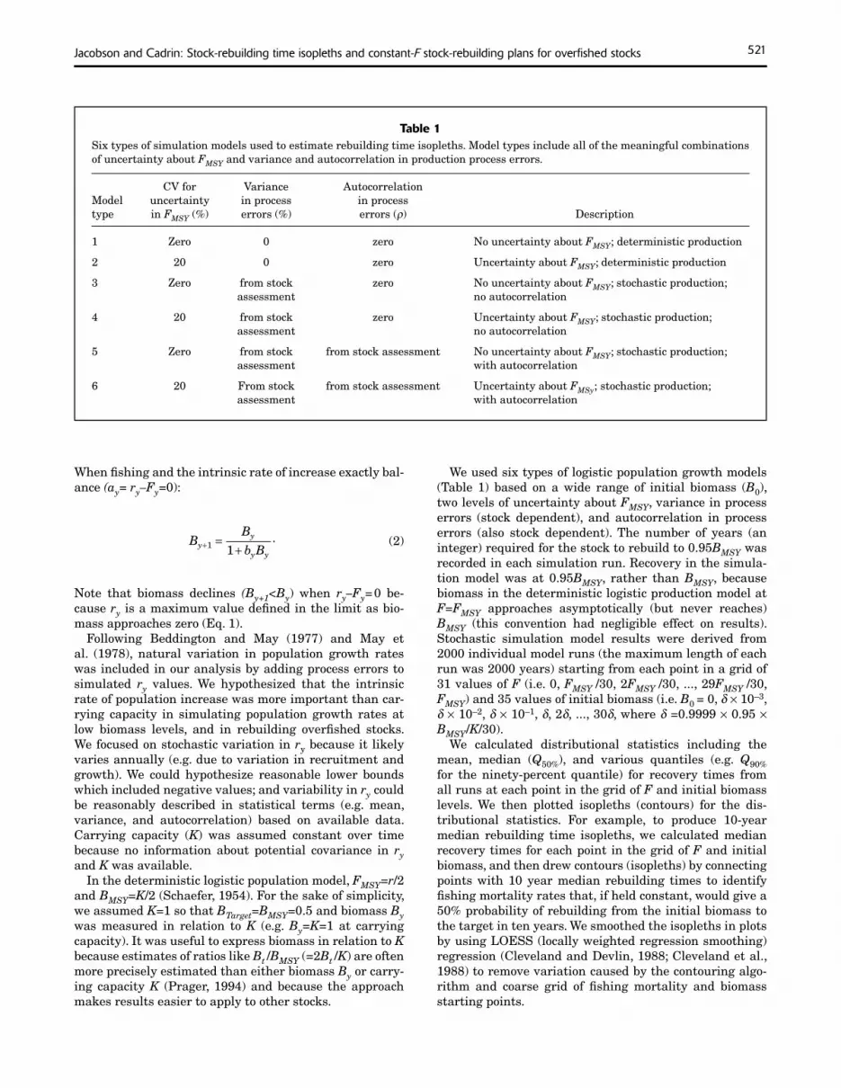
Table 2 Summary statistics and gamma distribution parameters for annual process errors in the intrinsic population growth rate (ry) for Georges Bank yellowtail flounder (Limanda ferruginea), estimated from stock assessment results (Cadrin5 in the main text). Parameters α and β were estimated with fixed γ = –M by maximum likelihood. According to Cadrin,5 the carrying capacity is K=99,000 metric tons (t) (95% confidence interval 84,500–103,000 t).

Parameter K=84,500 t K=99,400 t K=103,000 t

Number By values ≤95% K 25 25 Sample mean 0.58 0.65 0.58 Sample variance 0.036 0.037 0.036 Autocorrelation ρ 0.34 0.34 α 15.7 15.7 β 0.0498 0.0499 γ = –M –0.2 –0.2 Mean 0.65 0.58 Variance 0.039 0.039 Mode 0.61 0.53

25

0.33 17.5

0.0488 –0.2

0.58 0.039 0.53

ry = Gy + Ry − M (7)

where Gy = the instantaneous rate of somatic growth; and

Ry = an instantaneous rate for recruitment (in units of biomass).

Somatic growth and recruitment may be density dependent but are usually positive (Gy≥0 and Ry≥0). Thus, ry=–M is possible in the extreme case of zero growth and zero recruitment.

Production process errors were simulated by drawing random numbers from a three-parameter gamma probability distribution (Johnson et al., 1994, Appendix 1). Runs with autocorrelated process errors used one of two algorithms based on gamma distributions with adjusted parameter estimates (Appendix 2).

Georges Bank yellowtail flounder

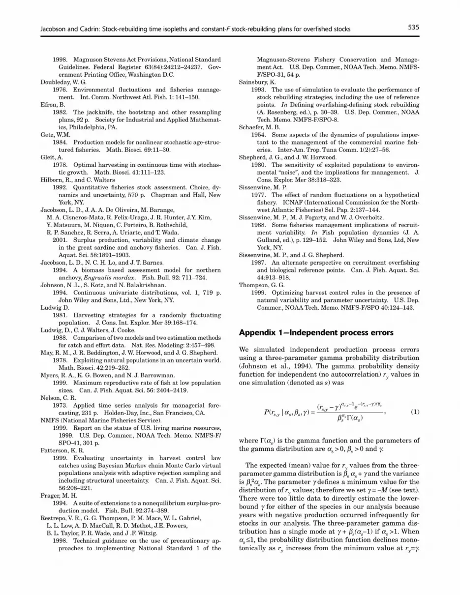
Cadrin5 used virtual population analysis (VPA, calibrated by using survey data) to estimate stock biomass for Georges Bank yellowtail flounder during 1973–98. In the same assessment, a surplus production model (ASPIC [stock-production model incorporating covariates], Prager, 1994) was used to estimate K=93,700 metric tons (t) (80% bootstrap confidence interval 87,700–97,000 t) and FMSY=0.30/yr (80% bootstrap confidence interval 0.27– 0.32/yr).

Cadrin’s stock assessment5 and our production calculations indicate that Georges Bank yellowtail flounder is a moderately long-lived (maximum observed age 14 yr,

5 Cadrin, S. X. 2000. Georges Bank yellowtail flounder. In Northern demersal working group: assessment of 11 northeast groundfish stocks through 1999. In Northeast Fisheries Science Center Reference Document 00-05, p. 45–64. Northeast Fisheries Science Center 166 Water Street, Woods Hole, MA, 02543.

assumed M=0.2 /yr), relatively productive (r=0.58–0.65) stock with some autocorrelation (ρ=0.33–0.34) in production process errors (Table 2). Empirical, and gamma distributions fit by maximum likelihood and the method of moments had similar means and variances (Table 2). Surplus production and biomass are related for Georges Bank yellowtail flounder, with Py reduced at the low By levels (Fig. 2A). Variability in estimated ry values indicate autocorrelation in process errors (Fig. 2B). The distribution of ry values (Fig. 2C) was skewed to the left and there were no negative values. Gamma distributions fitted by maximum likelihood and the method of moments (Appendix 1) were similar in shape (Fig. 2C). In simulations for yellowtail flounder, we used FMSY=0.30 (from ASPIC) with σ r

2 y = 0.037 and ρ= 0.33.

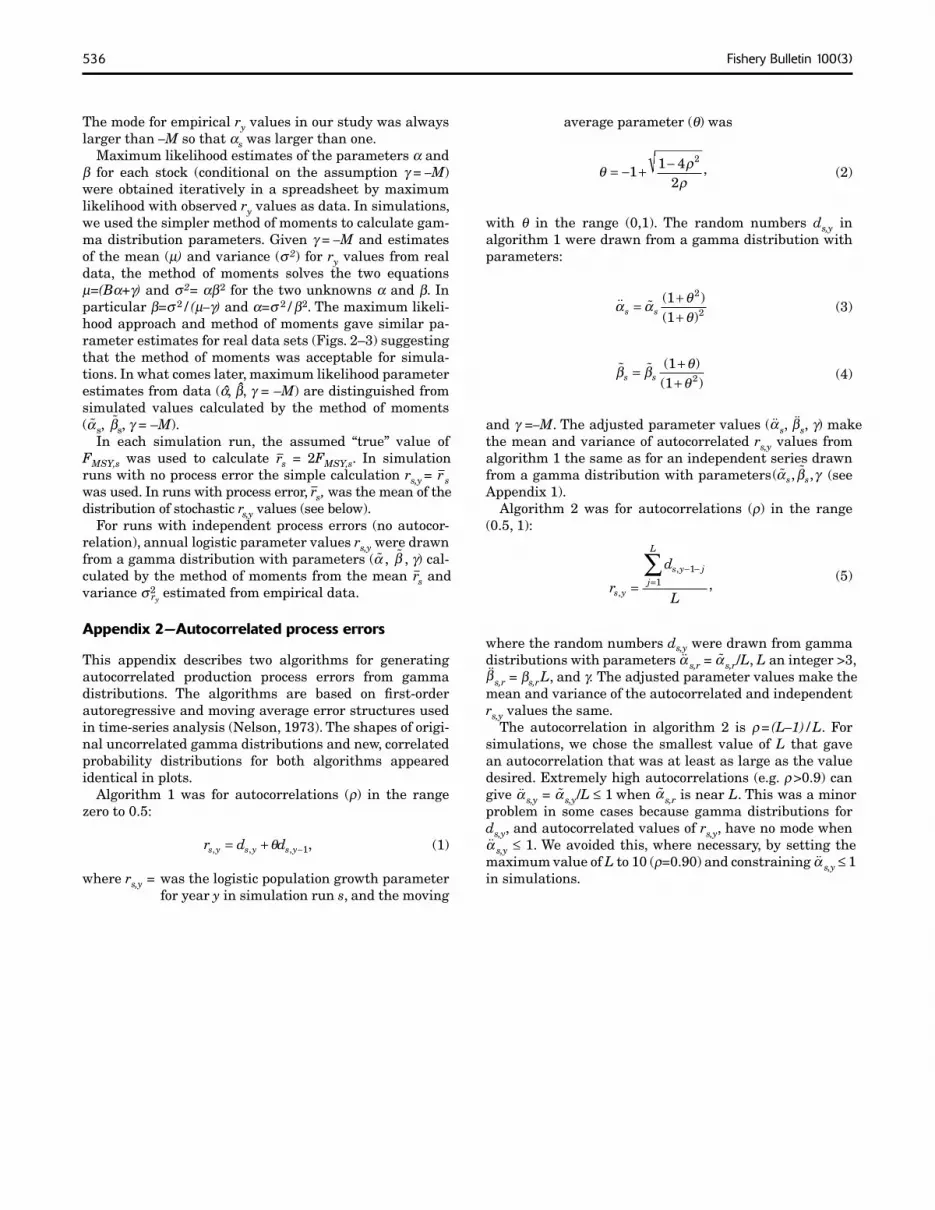
Cowcod rockfish

Butler et al.6 (see also Butler et al.7) estimated K=3400 t (95% CI 2800–4000 t) with a delay-difference biomass dynamic model for cowcod rockfish in the Southern California Bight. Annual biomass estimates from the same source were used to calculate surplus production during 1951–97 when the stock was fished down from about 3200 t to 240 t (about 7% of virgin biomass).

Butler et al.6 and our production calculations indicate that cowcod rockfish are a long-lived (maximum observed

6 Butler, J. L., L. D. Jacobson, J. T. Barnes, and H. G. Moser. 2002. Manuscript in revew. Biology and population dynamics of cowcod rockfish (Sebastes levis) in the southern California Bight.

7 Butler, J. L., L. D. Jacobson, J. T. Barnes, H. G. Moser, and R. Collins. 1999. Stock assessment of cowcod. In Appendix to the state of the Pacific Coast groundfish fishery through 1999 and recommended acceptable biological catch for 2000 stock assessment and fishery evaluation, p. Vi–113 (section 5). Pacific Fishery Management Council, 7700 NE Ambassador Place, Portland, OR, 97220-1384.


Figure 2 (A) Surplus production estimates Py and biomass estimates By for Georges Bank yellowtail flounder during 1973–97. The biomass estimates and parabolic curve fitted to production estimates are from Cadrin.5 (B) Time series of annual intrinsic rate of growth (ry) parameter value estimates from Equation 6. (C) Probability distributions for ry values used in simulations for Georges Bank yellowtail flounder.

Sur

plus

pro

duct

ion

Intr

insi

c po

pula

tion

grow

th r

ate

(ry)

Pro

babi

lity

Stock biomass (t)

Year

Intrinsic population growth rate (ry)

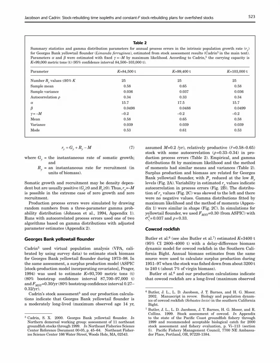
Figure 3 (A) Surplus production estimates Py and biomass estimates By from Butler et al.6

for cowcod rockfish during 1951–97 in the Southern California Bight. The parabolic curve fitted to production estimates (Py) shows trends only and is not recommended for management purposes. (B) Time series of annual intrinsic rate of growth (ry) parameter value estimates from Equation 6. (C) Probability distributions for ry values used in simulations for cowcod rockfish.

Sur

plus

pro

duct

ion

Intr

insi

c po

pula

tion

grow

th r

ate

(ry)

Pro

babi

lity

Intrinsic population growth rate (ry)

Stock biomass (t)

Year

age 55 yr, assumed M=0.055/yr), relatively unproductive stock (ry=0.027–0.037). Cowcod rockfish are much less pro- no clear relationship between surplus production and bioductive than Georges Bank yellowtail flounder because mass, but Py was lowest at the highest and lowest By levof their long lives and slower growth and because adult els and autocorrelation in production process errors was habitat is limited to steep rocky areas in relatively deep obvious (Fig. 3A). The distribution of ry values (Fig. 3B) water (90–500 m, Butler et al.6). Production process errors was skewed to the right and there were no negative valshow a high level of autocorrelation (ρ=0.83–0.94, Table ues. Gamma distributions fitted by maximum likelihood 3). Means, variances and autocorrelations for ry were not and the method of moments (Appendix 1) were similar in very sensitive to assumptions about K (Table 3). There was shape (Fig. 3).


Table 3 Summary statistics and gamma distribution parameters for annual process errors in the intrinsic population growth rate (ry) for cowcod rockfish (Sebastes levis), estimated from stock assessment results (Butler et al.6). Parameters α and β, were estimated with fixed γ = –M by maximum likelihood. K is the carrying capacity in the logistic population dynamics model. According to Butler et al.,6 K=3400 metric tons (t) (95% confidence interval 2800–4000 t).

Parameter K=84,500 t K=99,400 t K=103,000 t

Number By values ≤95% K 31 47 Sample mean 0.037 0.039 0.027 Sample variance 0.00059 0.00050 0.00021 Autocorrelation ρ 0.83 0.89 α –0.055 –0.055 β 17.7 36.1 γ = –M 0.0052 0.0023 Mean 0.039 0.027 Variance 0.00047 0.00019 Mode 0.034 0.025

47

0.94 –0.055 19.0 0.0049

0.037 0.00048

0.032

With K=3400 t (Table 3), r = 0.039 which suggests FMSY = 0.0185/yr. This crude estimate is less than implied by the simple calculation r = 2FMSY = 0.11 based on the proxy FMSY = M = 0.055/yr, possibly because the natural mortality rate overestimates FMSY for cowcod (Deriso, 1982). ASPIC estimates were similar (FMSY = 0.018/yr with an 80% bootstrap confidence interval 0.00082–0.039/yr) to estimates based on ry. In simulations for cowcod, we used F̂ MSY=0.018 (from ASPIC), σ2

ry = 0.00050 and ρ=0.9.

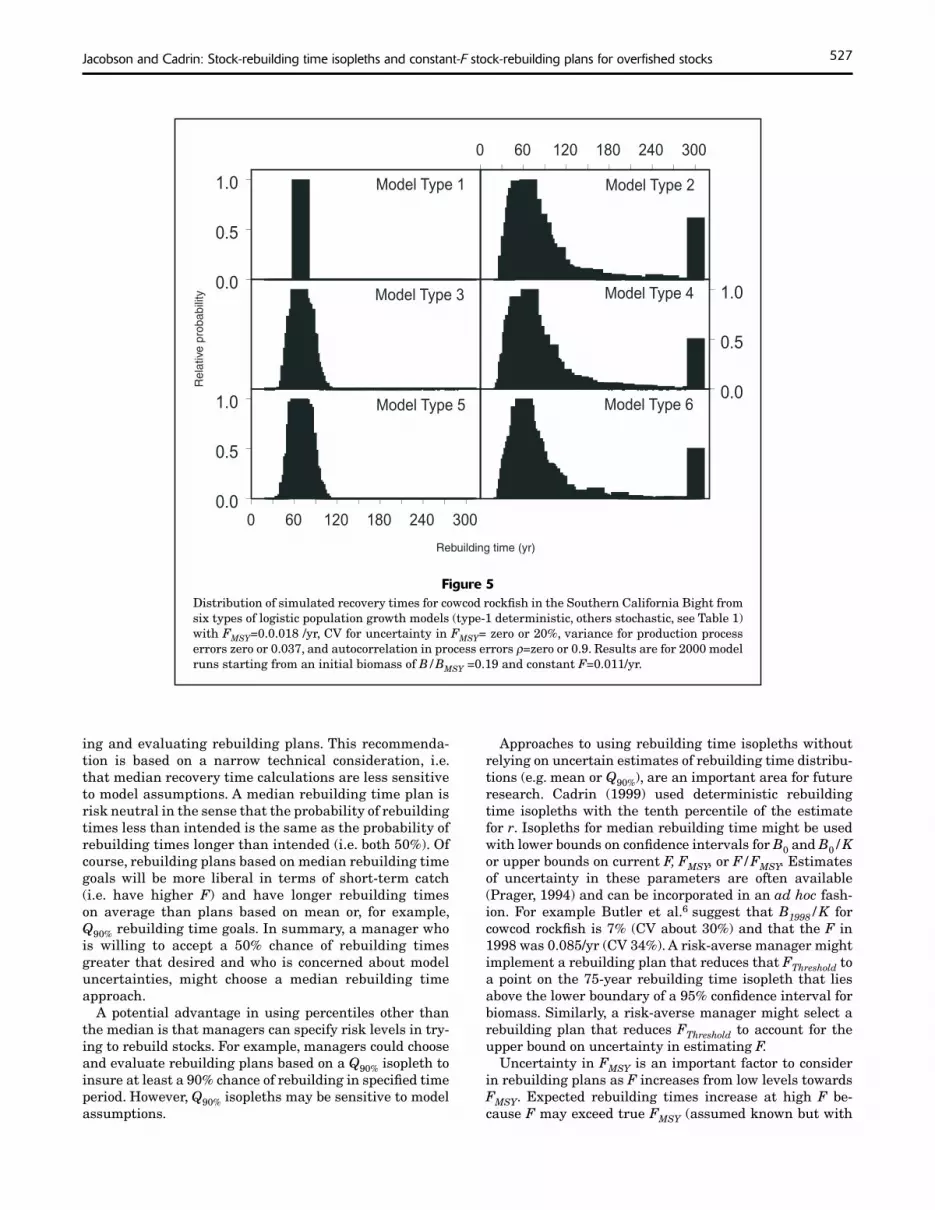
Simulation model runs indicated that cowcod are very unlikely to rebuild to BMSY in ten years. The mean generation time for cowcod is about 35 years (calculated as described by Restrepo et al., 1998). Simulations indicate that the mean time for rebuilding the stock with zero F is approximately 40 years (30–50 years, depending on model type). In accord with National Standard 1 Guidelines, it may be reasonable to develop plans with the goal of rebuilding the cowcod stock in 75 years or less. We therefore calculated and plotted 75-year, rather than 10-year rebuilding time isopleths, for cowcod rockfish.

Sensitivity analyses

We conducted three sensitivity analyses for each stock to determine if the choice of statistical distribution for stochastic rs,y values influenced rebuilding times in simulations. Sensitivity analyses used uncorrelated process errors and no uncertainty in FMSY (model type 3). The first sensitivity analysis run for each stock was a nonparametric bootstrap (Efron, 1982) with rs,y values drawn randomly with replacement from the observed values (Eq. 6). The second and third sensitivity analyses run for each stock were parametric bootstraps with rs,y values drawn from a normal or lognormal distribution with the same mean (µ) and variance (σ 2) as the observed values (Tables 2–3, Figs. 2–3). To avoid bias in runs with the lognormal

distribution (Beauchamp and Olson, 1973), log-transformed rs,y values were drawn from a normal distribution with mean ln(µ)–τ2/2 and variance τ 2=ln(CV2+1), with CV= σ/µ (Jacobson et al., 1994). For convenience in programming, rs,y values in normal and lognormal runs were sampled with replacement from a fixed pool of 200 random numbers drawn from the proper statistical distribution at the outset of the simulation.

Results

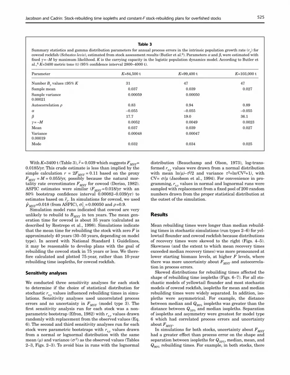
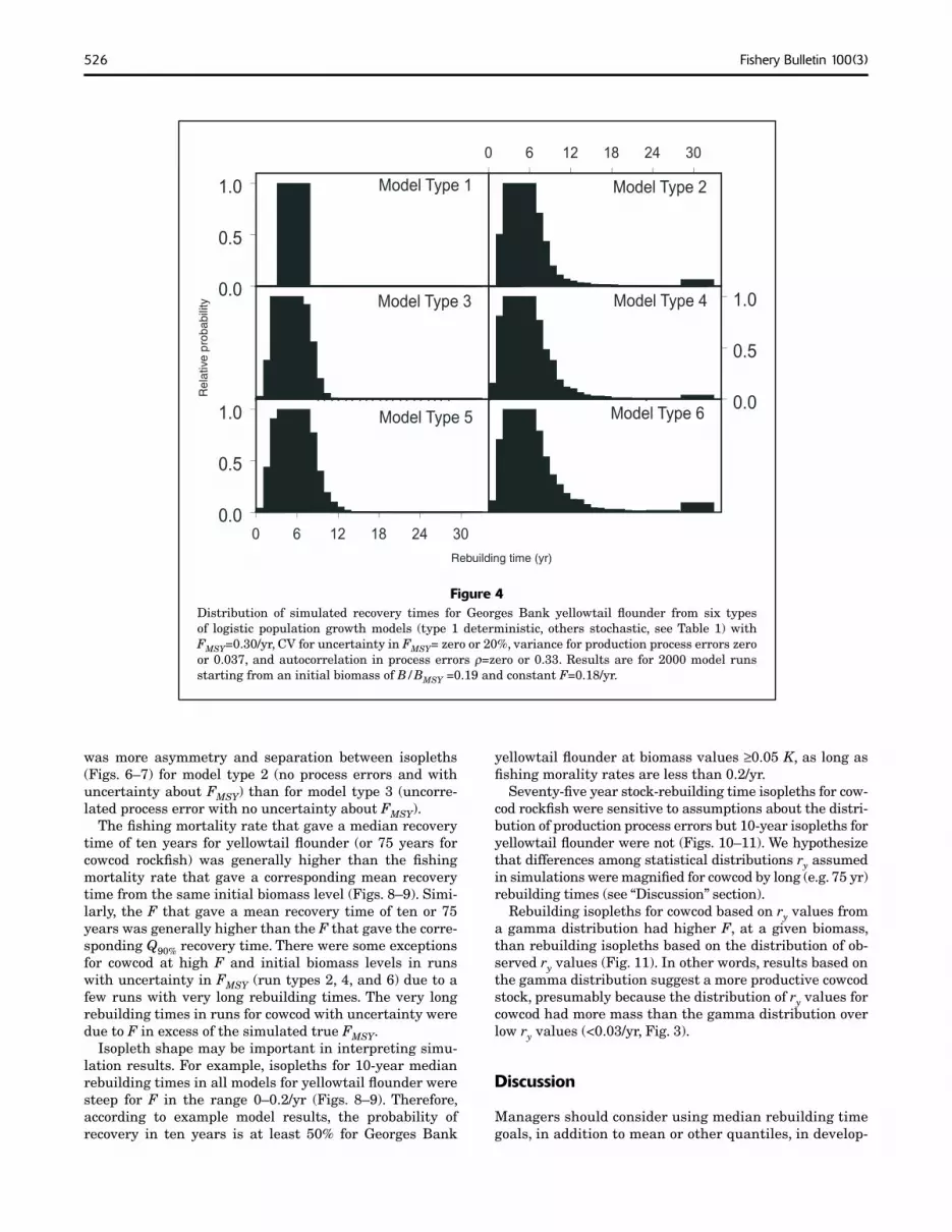
Mean rebuilding times were longer than median rebuilding times in stochastic simulations (run types 2–6) for yellowtail flounder and cowcod rockfish because distributions of recovery times were skewed to the right (Figs. 4–5). Skewness (and the extent to which mean recovery times exceeded median recovery times) was more pronounced at lower starting biomass levels, at higher F levels, where there was more uncertainty about FMSY and autocorrelation in process errors.

Skewed distributions for rebuilding times affected the shape of rebuilding time isopleths (Figs. 6–7). For all stochastic models of yellowtail flounder and most stochastic models of cowcod rockfish, isopleths for mean and median rebuilding times were widely separated. In addition, isopleths were asymmetrical. For example, the distance between median and Q90% isopleths was greater than the distance between Q10% and median isopleths. Separation of isopleths and asymmetry were greatest for model type 6 which had correlated process errors and uncertainty about FMSY.

In simulations for both stocks, uncertainty about FMSY had a greater effect than process error on the shape and separation between isopleths for Q10%, median, mean, and Q90% rebuilding times. For example, in both stocks, there


Figure 4 Distribution of simulated recovery times for Georges Bank yellowtail flounder from six types of logistic population growth models (type 1 deterministic, others stochastic, see Table 1) with FMSY=0.30/yr, CV for uncertainty in FMSY= zero or 20%, variance for production process errors zero or 0.037, and autocorrelation in process errors ρ=zero or 0.33. Results are for 2000 model runs starting from an initial biomass of B/BMSY =0.19 and constant F=0.18/yr.

0 12 18 24 30

0 12 18 24 30

Rebuilding time (yr)

Rel

ativ

e pr

obab

ility

0.0

0.5

1.0

0.0

0.5

1.0

0.0

0.5

1.0

Model Type 1 Model Type 2


Model Type 6Model Type 5

6

6

was more asymmetry and separation between isopleths (Figs. 6–7) for model type 2 (no process errors and with uncertainty about FMSY) than for model type 3 (uncorrelated process error with no uncertainty about FMSY).

The fishing mortality rate that gave a median recovery time of ten years for yellowtail flounder (or 75 years for cowcod rockfish) was generally higher than the fishing mortality rate that gave a corresponding mean recovery time from the same initial biomass level (Figs. 8–9). Similarly, the F that gave a mean recovery time of ten or 75 years was generally higher than the F that gave the corresponding Q90% recovery time. There were some exceptions for cowcod at high F and initial biomass levels in runs with uncertainty in FMSY (run types 2, 4, and 6) due to a few runs with very long rebuilding times. The very long rebuilding times in runs for cowcod with uncertainty were due to F in excess of the simulated true FMSY.

Isopleth shape may be important in interpreting simulation results. For example, isopleths for 10-year median rebuilding times in all models for yellowtail flounder were steep for F in the range 0–0.2/yr (Figs. 8–9). Therefore, according to example model results, the probability of recovery in ten years is at least 50% for Georges Bank

yellowtail flounder at biomass values ≥0.05 K, as long as fishing morality rates are less than 0.2/yr.

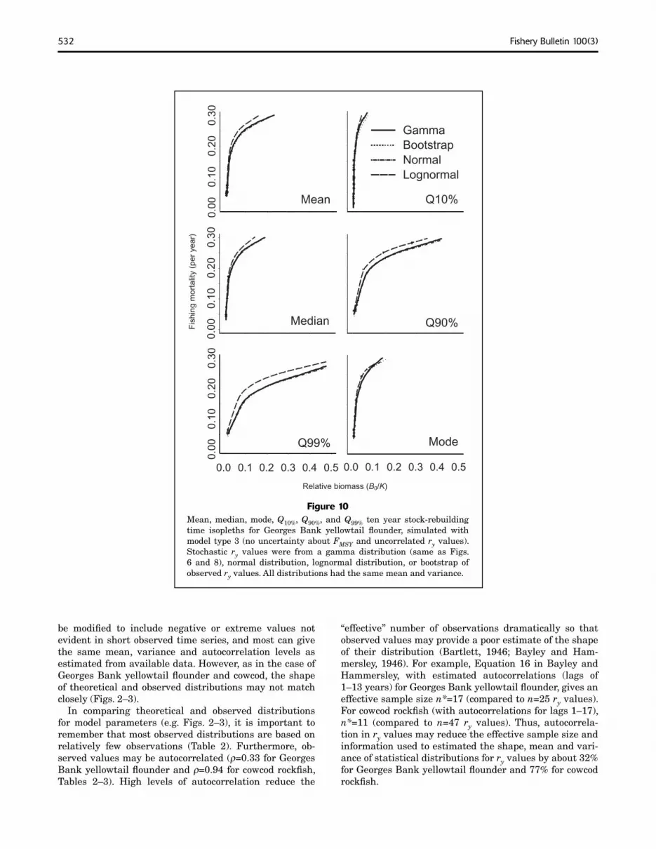
Seventy-five year stock-rebuilding time isopleths for cowcod rockfish were sensitive to assumptions about the distribution of production process errors but 10-year isopleths for yellowtail flounder were not (Figs. 10–11). We hypothesize that differences among statistical distributions ry assumed in simulations were magnified for cowcod by long (e.g. 75 yr) rebuilding times (see “Discussion” section).

Rebuilding isopleths for cowcod based on ry values from a gamma distribution had higher F, at a given biomass, than rebuilding isopleths based on the distribution of observed ry values (Fig. 11). In other words, results based on the gamma distribution suggest a more productive cowcod stock, presumably because the distribution of ry values for cowcod had more mass than the gamma distribution over low ry values (<0.03/yr, Fig. 3).

Discussion

Managers should consider using median rebuilding time goals, in addition to mean or other quantiles, in develop-

527Jacobson and Cadrin: Stock-rebuilding time isopleths and constant-F stock-rebuilding plans for overfi shed stocks

ing and evaluating rebuilding plans. This recommenda-tion is based on a narrow technical consideration, i.e. that median recovery time calculations are less sensitive to model assumptions. A median rebuilding time plan is risk neutral in the sense that the probability of rebuilding times less than intended is the same as the probability of rebuilding times longer than intended (i.e. both 50%). Of course, rebuilding plans based on median rebuilding time goals will be more liberal in terms of short-term catch (i.e. have higher F) and have longer rebuilding times on average than plans based on mean or, for example, Q90% rebuilding time goals. In summary, a manager who is willing to accept a 50% chance of rebuilding times greater that desired and who is concerned about model uncertainties, might choose a median rebuilding time approach.

A potential advantage in using percentiles other than the median is that managers can specify risk levels in try-ing to rebuild stocks. For example, managers could choose and evaluate rebuilding plans based on a Q90% isopleth to insure at least a 90% chance of rebuilding in specifi ed time period. However, Q90% isopleths may be sensitive to model assumptions.

Approaches to using rebuilding time isopleths without relying on uncertain estimates of rebuilding time distribu-tions (e.g. mean or Q90%), are an important area for future research. Cadrin (1999) used deterministic rebuilding time isopleths with the tenth percentile of the estimate for r. Isopleths for median rebuilding time might be used with lower bounds on confi dence intervals for B0 and B0/K or upper bounds on current F, FMSY, or F/FMSY. Estimates of uncertainty in these parameters are often available (Prager, 1994) and can be incorporated in an ad hoc fash-ion. For example Butler et al.6 suggest that B1998/K for cowcod rockfi sh is 7% (CV about 30%) and that the F in 1998 was 0.085/yr (CV 34%). A risk-averse manager might implement a rebuilding plan that reduces that FThreshold to a point on the 75-year rebuilding time isopleth that lies above the lower boundary of a 95% confi dence interval for biomass. Similarly, a risk-averse manager might select a rebuilding plan that reduces FThreshold to account for the upper bound on uncertainty in estimating F.

Uncertainty in FMSY is an important factor to consider in rebuilding plans as F increases from low levels towards FMSY. Expected rebuilding times increase at high F be-cause F may exceed true FMSY (assumed known but with

Figure 5Distribution of simulated recovery times for cowcod rockfi sh in the Southern California Bight from six types of logistic population growth models (type-1 deterministic, others stochastic, see Table 1) with FMSY=0.0.018 /yr, CV for uncertainty in FMSY= zero or 20%, variance for production process errors zero or 0.037, and autocorrelation in process errors ρ=zero or 0.9. Results are for 2000 model runs starting from an initial biomass of B/BMSY =0.19 and constant F=0.011/yr.

0 0 120 180 40 300

0 0 120 180 240 300

0.0

0.5

1.0

0.0

0.5

1.0

0.0

0.5

1.0

Model Type 1


Model Type 4

Model Type 2

Model Type 3

Rebuilding time (yr)

Rel

ativ

e pr

obab

ility

6 2

6


Figure 6Isopleths for mean, median, mode, Q10%, Q90%, and Q99% ten-year stock-rebuilding times simulated with six model types (Table 1) for Georges Bank yellowtail fl ounder. Isopleths for all statistics and one type of model are shown in each panel. Model types 2, 4, and 6 include uncer-tainty in FMSY.

error) in a high proportion of cases (Figs. 8–9). Fortunately, process errors and autocorrelation may reduce this prob-lem because stock growth rates increase in some years so that the true FMSY exceeds the manager’s estimate.

Stock-rebuilding times calculated with deterministic models approximate median rebuilding times from sto-chastic models. For example, rebuilding times in Cadrin (1999) calculated with a deterministic model for Georges Bank yellowtail fl ounder are very close to median rebuild-ing times from our stochastic models. From our results, we hypothesize that rebuilding time isopleths for other species (Applegate et al.3) based on Cadrin’s (1999) deter-ministic model should also be viewed as approximations to isopleths for median rebuilding times.

Our simulation analyses indicate that rebuilding times for overfi shed stocks (with a range of life history charac-

teristics, initial biomass levels and fi shing mortality rates) tend to be skewed and can be highly variable (Figs. 4–5). Hence, rebuilding in any specifi c case may be quicker or take much longer than expected, particularly if expecta-tions are based on deterministic models that approximate median rebuilding times. For example, probabilities of re-building times twice as long as the goal for Georges Bank yellowtail fl ounder (10 yr) and cowcod (75 yr) were 4% and 8% and probabilities of rebuilding times half as long were 40% and 1%.

Modeling choices

Stochastic models are necessary when estimates of mean rebuilding times or quantiles other than the deterministic approximation to the median are needed. Rebuilding time

0.0 0.1 0.2 0.3 0.4 0.5

Mode

0.00

0.10

0.20

0.30

Mean

Q90%

0.0 0.1 0.2 0.3 0.4 0.5

0.00

0.10

0.20

0.30

Q99%

Q10%

Model 1Model 2Model 3Model 4Model 5Model 6

0.00

0.10

0.20

0.30

Median

Relative biomass (B0/K)

Fis

hing

mor

talit

y (p

er y

ear)


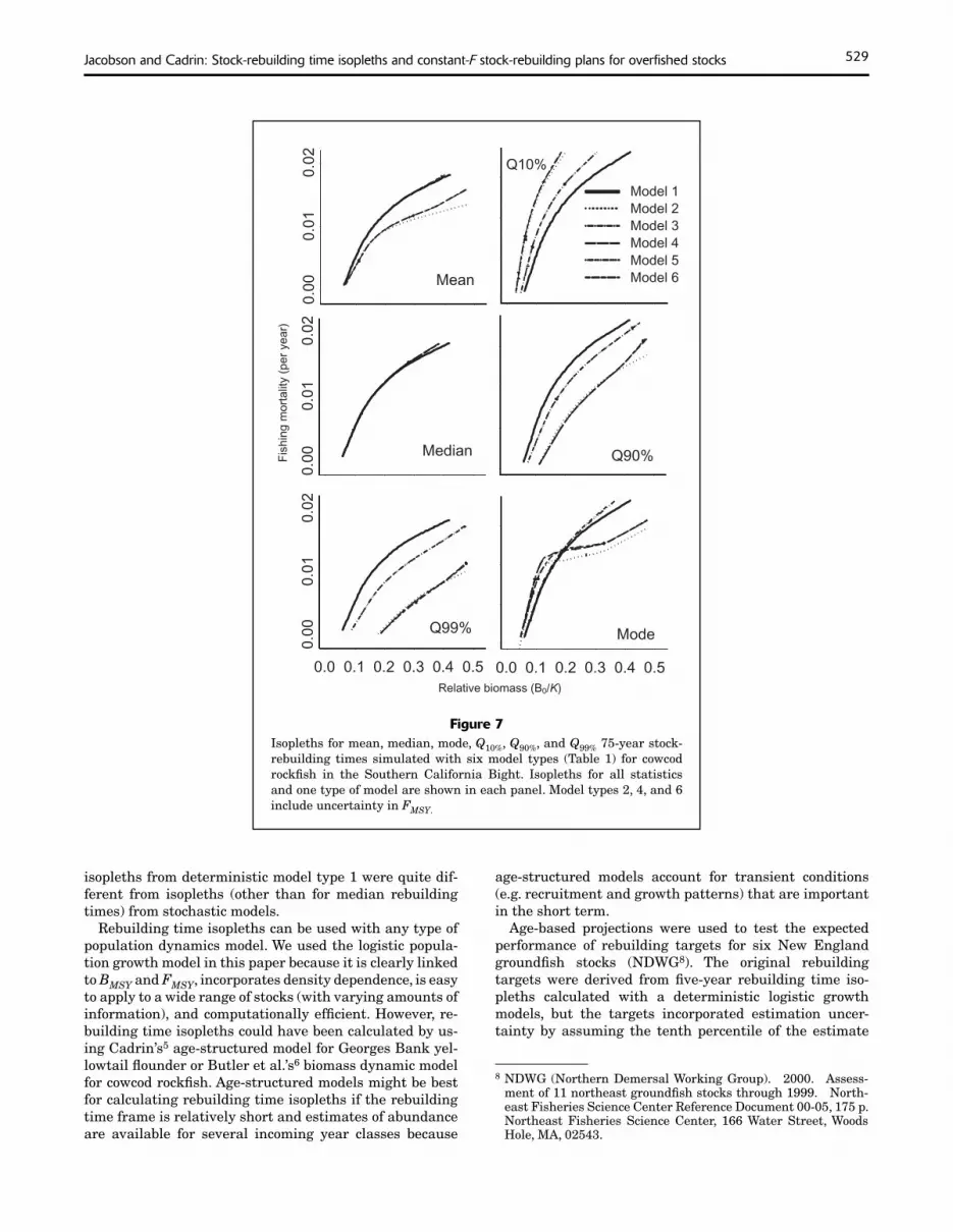
Figure 7Isopleths for mean, median, mode, Q10%, Q90%, and Q99% 75-year stock-rebuilding times simulated with six model types (Table 1) for cowcod rockfi sh in the Southern California Bight. Isopleths for all statistics and one type of model are shown in each panel. Model types 2, 4, and 6 include uncertainty in FMSY.

isopleths from deterministic model type 1 were quite dif-ferent from isopleths (other than for median rebuilding times) from stochastic models.

Rebuilding time isopleths can be used with any type of population dynamics model. We used the logistic popula-tion growth model in this paper because it is clearly linked to BMSY and FMSY, incorporates density dependence, is easy to apply to a wide range of stocks (with varying amounts of information), and computationally effi cient. However, re-building time isopleths could have been calculated by us-ing Cadrin’s5 age-structured model for Georges Bank yel-lowtail fl ounder or Butler et al.’s6 biomass dynamic model for cowcod rockfi sh. Age-structured models might be best for calculating rebuilding time isopleths if the rebuilding time frame is relatively short and estimates of abundance are available for several incoming year classes because

age-structured models account for transient conditions (e.g. recruitment and growth patterns) that are important in the short term.

Age-based projections were used to test the expected performance of rebuilding targets for six New England groundfi sh stocks (NDWG8). The original rebuilding targets were derived from fi ve-year rebuilding time iso-pleths calculated with a deterministic logistic growth models, but the targets incorporated estimation uncer-tainty by assuming the tenth percentile of the estimate

8 NDWG (Northern Demersal Working Group). 2000. Assess-ment of 11 northeast groundfi sh stocks through 1999. North-east Fisheries Science Center Reference Document 00-05, 175 p.Northeast Fisheries Science Center, 166 Water Street, Woods Hole, MA, 02543.

Model 1Model 2Model 3Model 4Model 5Model 6

Q10%

0.0 0.1 0.2 0.3 0.4 0.5

0.00

0.01

0.02

Q99%

0.00

0.01

0.02

Median

Q90%

0.00

0.01

0.02

Mean

0.0 0.1 0.2 0.3 0.4 0.5

Mode


Fis

hing

mor

talit

y (p

er y

ear)


Figure 8Isopleths for mean, median, mode, Q10%, Q90%, and Q99% ten-year stock-rebuilding times simulated with six model types (Table 1) for Georges Bank yellowtail fl ounder. Isopleths for one statistic and all six model types are shown in each panel. Isopleths of mean and modal rebuilding times in results for models with uncertainty in FMSY (model types 2, 4, and 6) may be distorted (fl at) at relatively high fi shing mortality levels because fi shing mortality exceeds the simulated true FMSY in some simulations, so that the simulated stock may never rebuild.

of r (Cadrin, 1999; Applegate et al.3). For the six stocks, starting biomass in 1999 ranged from 25% to 93% of BMSY and estimates of FMSY ranged from 0.5 to 0.8. Estimated rebuilding times averaged 3.5 years (ranging from 1 to 7 yr) for 50% probability of attaining BMSY (NDWG8). There-fore, the age-based simulations indicated that isopleths based on deterministic biomass dynamic models generally performed well for overfi shed New England groundfi sh stocks. Brodziak et al. (2001) analyzed stock-recruit data and concluded that “(1) time horizons for rebuilding will be uncertain, owing to recruitment variability, (2) some productive stocks (haddock, yellowtail fl ounder) have seri-al correlation in recruitment and this may either enhance

or diminish chances for stock recovery.” Thus, results with surplus production models, age-structured models, and stock-recruit analyses highlight the fundamental similarities between a wide range of modeling approaches (Sissenwine and Shepherd, 1987).

The best choice of stochastic simulation model for devel-oping and evaluating rebuilding plans will depend on the situation. Sainsbury (1993) concluded that models incor-porating simple assumptions about population dynamics were more appropriate for evaluating performance of con-trol rules than models with more complex assumptions. PFMC1 used a simple model incorporating environmental effects on recruitment with useful results. However, Bell

0.0 0.1 0.2 0.3 0.4 0.5

Model Type 6

0.0 0.1 0.2 0.3 0.4 0.5

0.00

0.10

0.20

0.30

Model Type 5

Model Type 20.

000.

100.

200.

30

Model Type 3

0.00

0.10

0.20

0.30

Model Type 1

MeanQ10%MedianQ90%Q99%Mode

Model Type 4


Fis

hing

mor

talit

y (p

er y

ear)


Figure 9 Isopleths for mean, median, mode, Q10%, Q90%, and Q99% 75-year stockrebuilding times simulated with six model types (Table 1) for cowcod rockfish in the Southern California Bight. Isopleths for one statistic and all six model types are shown in each panel. Model types 2, 4, and 6 include uncertainty in FMSY. Isopleths of mean and modal rebuilding times in results for models with uncertainty in FMSY (model types 2, 4, and 6) may be distorted (flat) at relatively high fishing mortality levels because fishing mortality exceeds the simulated true FMSY in some simulations so that the simulated stock may never rebuild.

Fis

hing

mor

talit

y (p

er y

ear)


and Stefansson9 and Patterson (1999) used more complex simulation models with success.

Distributional assumptions

Simulation analyses (Figs. 10–11) indicate that the choice of statistical distribution for simulating process errors in model parameters (e.g. ry) may be important,

9 Bell, E. D., and G. Stefansson. 1998. Performance of some harvest control rules. NAFO (North Atlantic Fisheries Organization) SCR Doc. 98/7, 1–19. Northwest Atlantic Fisheries Organization, 2 Morris Drive, P. O. Box 638, Dartmouth, Nova Scotia, B2Y 3Y9, Canada.

particularly when rebuilding times are long (e.g. those for cowcod rockfish) due to low stock productivity, low stock biomass, unproductive stock dynamics, or autocorrelation in process errors. The choice of statistical distributions for simulating ry involves choosing between theoretical distributions supported by theory (e.g. autocorrelated gamma distribution with negative values bounded below at –M) or bootstrap distributions of observed values. The programming and work required to experiment with alternative distributions is not overwhelming and we recommend sensitivity analyses in cases where distributional assumptions may be important.

Theoretical distributions for stochastic parameters are flexible because many types of distributions are available, most can be modified to include autocorrelation, most can


Figure 10Mean, median, mode, Q10%, Q90%, and Q99% ten year stock-rebuilding time isopleths for Georges Bank yellowtail fl ounder, simulated with model type 3 (no uncertainty about FMSY and uncorrelated ry values). Stochastic ry values were from a gamma distribution (same as Figs. 6 and 8), normal distribution, lognormal distribution, or bootstrap of observed ry values. All distributions had the same mean and variance.

be modifi ed to include negative or extreme values not evident in short observed time series, and most can give the same mean, variance and autocorrelation levels as estimated from available data. However, as in the case of Georges Bank yellowtail fl ounder and cowcod, the shape of theoretical and observed distributions may not match closely (Figs. 2–3).

In comparing theoretical and observed distributions for model parameters (e.g. Figs. 2–3), it is important to remember that most observed distributions are based on relatively few observations (Table 2). Furthermore, ob-served values may be autocorrelated (ρ=0.33 for Georges Bank yellowtail fl ounder and ρ=0.94 for cowcod rockfi sh, Tables 2–3). High levels of autocorrelation reduce the

“effective” number of observations dramatically so that observed values may provide a poor estimate of the shape of their distribution (Bartlett, 1946; Bayley and Ham-mersley, 1946). For example, Equation 16 in Bayley and Hammersley, with estimated autocorrelations (lags of 1–13 years) for Georges Bank yellowtail fl ounder, gives an effective sample size n*=17 (compared to n=25 ry values). For cowcod rockfi sh (with autocorrelations for lags 1–17), n*=11 (compared to n=47 ry values). Thus, autocorrela-tion in ry values may reduce the effective sample size and information used to estimated the shape, mean and vari-ance of statistical distributions for ry values by about 32% for Georges Bank yellowtail fl ounder and 77% for cowcod rockfi sh.

0.0 0.1 0.2 0.3 0.4 0.5

0.00

0.10

0.20

0.30

Q99%

Q10%

Gamma BootstrapNormalLognormal

0.00

0.10

0.20

0.30

Median

0.00

0.10

0.20

0.30

Mean

Q90%

0.0 0.1 0.2 0.3 0.4 0.5

Mode

Fis

hing

mor

talit

y (p

er y

ear)



Developing, monitoring, and evaluating stock-rebuilding programs

Once the management goal, desired probability of achiev-ing the stock-rebuilding goal, and the time frame for rebuilding are identifi ed (e.g.10-yr median rebuilding time to a BMSY target), the simplest way to use stock-rebuilding time isopleths in designing a rebuilding plan is to choose a constant-F̃B0

level from the appropriate rebuilding time isopleth, based on a current estimate of B0. Cadrin (1999) has provided an example of this approach.

Stock-rebuilding time isopleths can be used to monitor the progress of any rebuilding plan although interpreta-tion is clearest with constant-F values (Cadrin, 1999). For example, the point defi ned by current biomass and F for Georges Bank yellowtail fl ounder in the second year

(1997) of a hypothetical fi ve-year rebuilding plan begin-ning in 1996 should lie near or within the 3-year rebuild-ing time isopleth (Fig. 1). If the point lies far outside the 3-year isopleth, then managers could be sure that the rebuilding plan was behind schedule.

Evaluating harvest control rules as stock-rebuilding programs

It may be necessary to evaluate harvest control rules that allow F to vary with biomass (e.g. the common harvest control rule in Fig. 1) as a rebuilding plan. Rebuilding isopleths provide guidance in this situation because they can be used to reject some harvest control rules based on a single necessary criterion. However, the test is weak because a harvest control rule that passes the test may or

0.00 0.25 0.50

0.00

0.01

0.02

Q99%

0.00

0.01

0.02

Mean

Gamma BootstrapNormalLognormal

0.00

0.01

0.02

Median

Q10%

Q90%

0.00 0.25 0.50

Mode

Fis

hing

mor

talit

y (p

er y

ear)


Figure 11Mean, median, mode, Q10%, Q90%, and Q99% 75-year stock-rebuilding time isopleths for cowcod rockfi sh, simulated with model type 3 (no uncer-tainty about FMSY and uncorrelated ry values). Stochastic ry values were from a gamma distribution (same as Figs. 7 and 9), normal distribution, lognormal distribution or bootstrap of observed ry values. All distribu-tions had the same mean and variance.


may not be sufficient as a rebuilding plan. In this context, it is important to remember that rebuilding time isopleths are constructed based on the assumption of constant fishing mortality rates during the rebuilding program. More complicated rebuilding plans, that allow F to vary according to changes in biomass or other factors, are best evaluated by stock-specific simulations.

The test is based on the notion that control rules that allow F levels above the stock-rebuilding time isopleth for biomass levels above B0 are unlikely to rebuild the stock with desired probability in the desired time frame. Therefore, as a minimum requirement for meeting rebuilding time goals, harvest control rules used as rebuilding plans should lie on or under the corresponding rebuilding time isopleth for all biomass levels above B0. Consider a hypothetical overfished stock for which there is a ten-year median rebuilding time goal. Assume that a harvest control rule proposed as a rebuilding plan has the typical shape (i.e. F increases or stays the same as biomass increases, as in Fig. 1). If the control rule lies above the isopleth for some critical biomass level between B0 and BMSY, then the rule will allow fishing mortality rates that are generally too high to meet management goals once biomass reaches the critical level.

The example of Georges Bank yellowtail flounder

Georges Bank yellowtail flounder (Fig. 1) can be used to illustrate how rebuilding time isopleths might have been used to evaluate stock-rebuilding plans for hypothetical implementation during 1996 and how stock-rebuilding time isopleths can be used to monitor progress in rebuilding overfished stocks. The discussion is hypothetical, however, because the examples evaluate management approaches that have not been used in rebuilding the stock. In reality, managers kept F for Georges Bank yellowtail flounder during 1996–99 nearly constant at a level well the below the 10-year isopleth, and the Georges Bank yellowtail flounder stock was almost rebuilt to the BMSY target level in 1999 after only four years (Fig. 1).

Based on this example, the harvest control rule in Figure 1 would have been marginal for use in a hypothetical median ten-year stock-rebuilding plan for Georges Bank yellowtail flounder starting in 1996, because the rule lies slightly above the 10-year isopleth for biomass levels of 47% BMSY. The harvest rule might have been rejected outright as a five-year rebuilding plan because the rule lies well above the 5-year rebuilding time isopleth. The rebuilding trajectory for Georges Bank yellowtail flounder (Fig. 1) shows that the five-year rebuilding plan, which began in 1996, was on schedule during 1996–98 because fishing mortality and estimated biomass were within the 5-year, 4-year, and 3-year isopleths during successive years.

The Georges Bank yellowtail flounder example provides an important final lesson about uncertainty in actual rebuilding times, even if statistical distributions of potential rebuilding times are characterized accurately. During 1996–99, the stock was managed at a relatively constant F level that was well above the entire 4-year median rebuilding time isopleth (Fig. 1). Despite the relatively high F level, Georges Bank yellowtail flounder reached a

biomass level near BMSY in 1999, after four years. We attribute this fortunate chain of events to stochastic variation in process errors stemming primarily from recruitment and growth of the strong 1997 year class (Cadrin5).

Acknowledgments

We thank P. Rago, D. Hart, M. Sissenwine (National Marine Fisheries Service, Woods Hole, MA), M. Prager (National Marine Fisheries Service, Beaufort, NC), and three anonymous reviewers for information and advice. S. Murawski suggested sensitivity analyses. J. Boreman, S. Murawski, and F. Serchuk (National Marine Fisheries Service, Woods Hole, MA) made editorial suggestions.

Literature cited

Bartlett, M. S. 1946. On the theoretical specifications and sampling prop

erties of autocorrelated time series. J. R. Stat. Soc. Ser. B (methodol.) 8:27–41.

Bayley, G. V., and J. M. Hammersley. 1946. The “effective” number of independent observations

in an autocorrelated time series. J. R. Stat. Soc. Ser. B (methodol.) 8:184–197.

Beauchamp, J., and J. Olson. 1973. Corrections for bias in regression estimates after log

arithmic transformation. Ecology (Washington DC) 54: 1403–1407.

Beddington, J. R., and R. M. May. 1977. Harvesting natural populations in a randomly fluctu

ating environment. Science 197: 463–465. Brodziak, J. K. T., W. J. Overholtz, and P. J. Rago.

2001. Does spawning stock affect recruitment of New England groundfish. Can. J. Fish. Aquat. Sci. 58: 306–318.

Cadrin, S. X. 1999. A precautionary approach to fishery control rules

based on surplus production modeling. In Proceedings of the fifth national NMFS stock assessment workshop (V. Restrepo, ed.), p. 17–22. U.S. Dep. Commer., NOAA Tech. Memo. NMFS-F/SPO-40.

Clark, W. G. 1991. Groundfish exploitation rate based on life history

parameters. Can. J. Fish. Aquat. Sci. 48:734–750. Cleveland, W. S., and S. J. Devlin.

1988. Locally weighted regression: an approach to regression analysis by local fitting. J. Am. Stat. Assoc. 83:596–610.

Cleveland, W. S., S. J. Devlin, and E. Grosse. 1988. Regression by local fitting: methods, properties and

computational algorithms. J. Econometrics 37:87–114. Dennis, B., and G. P. Patil.

1984. The gamma distribution and weighted multimodal gamma distributions as models of population abundance. Math. Biosci. 68:187–212.

Deriso, R. B. 1982. Relationship of fishing mortality and growth and the

level of maximum sustainable yield. Can. J. Fish. Aquat. Sci. 39:1054–1058.

DOC (Department of Commerce). 1996. Magnuson Stevens Fishery Conservation and Manage

ment Act as amended through October 11, 1996. U.S. Dep. Commer., NOAA Tech. Memo. NMFS-F/SPO-23, 121 p.


1998. Magnuson Stevens Act Provisions, National Standard Guidelines. Federal Register 63(84):24212–24237. Government Printing Office, Washington D.C.

Doubleday, W. G. 1976. Environmental fluctuations and fisheries manage

ment. Int. Comm. Northwest Atl. Fish. 1: 141–150. Efron, B.

1982. The jackknife, the bootstrap and other resampling plans, 92 p. Society for Industrial and Applied Mathematics, Philadelphia, PA.

Getz, W.M. 1984. Production models for nonlinear stochastic age-struc

tured fisheries. Math. Biosci. 69:11–30. Gleit, A.

1978. Optimal harvesting in continuous time with stochastic growth. Math. Biosci. 41:111–123.

Hilborn, R., and C. Walters 1992. Quantitative fisheries stock assessment. Choice, dy

namics and uncertainty, 570 p. Chapman and Hall, New York, NY.

Jacobson, L. D., J. A. A. De Oliveira, M. Barange, M. A. Cisneros-Mata, R. Felix-Uraga, J. R. Hunter, J.Y. Kim, Y. Matsuura, M. Niquen, C. Porteiro, B. Rothschild, R. P. Sanchez, R. Serra, A. Uriarte, and T. Wada.

2001. Surplus production, variability and climate change in the great sardine and anchovy fisheries. Can. J. Fish. Aquat. Sci. 58:1891–1903.

Jacobson, L. D., N. C. H. Lo, and J. T. Barnes. 1994. A biomass based assessment model for northern

anchovy, Engraulis mordax. Fish. Bull. 92: 711–724. Johnson, N .L., S. Kotz, and N. Balakrishnan.

1994. Continuous univariate distributions, vol. 1, 719 p. John Wiley and Sons, Ltd., New York, NY.

Ludwig D. 1981. Harvesting strategies for a randomly fluctuating

population. J. Cons. Int. Explor. Mer 39:168–174. Ludwig, D., C. J. Walters, J. Cooke.

1988. Comparison of two models and two estimation methods for catch and effort data. Nat. Res. Modeling: 2:457–498.

May, R. M., J. R. Beddington, J. W. Horwood, and J. G. Shepherd. 1978. Exploiting natural populations in an uncertain world.

Math. Biosci. 42:219–252. Myers, R. A., K. G. Bowen, and N. J. Barrowman.

1999. Maximum reproductive rate of fish at low population sizes. Can. J. Fish. Aquat. Sci. 56: 2404–2419.

Nelson, C. R. 1973. Applied time series analysis for managerial fore

casting, 231 p. Holden-Day, Inc., San Francisco, CA. NMFS (National Marine Fisheries Service).

1999. Report on the status of U.S. living marine resources, 1999. U.S. Dep. Commer., NOAA Tech. Memo. NMFS-F/ SPO-41, 301 p.

Patterson, K. R. 1999. Evaluating uncertainty in harvest control law

catches using Bayesian Markov chain Monte Carlo virtual populations analysis with adaptive rejection sampling and including structural uncertainty. Can. J. Fish. Aquat. Sci. 56:208–221.

Prager, M. H. 1994. A suite of extensions to a nonequilibrium surplus-pro

duction model. Fish. Bull. 92:374–389. Restrepo, V. R., G. G. Thompson, P. M. Mace, W. L. Gabriel,

L. L. Low, A. D. MacCall, R. D. Methot, J.E. Powers, B. L. Taylor, P. R. Wade, and J .F. Witzig.

1998. Technical guidance on the use of precautionary approaches to implementing National Standard 1 of the

Magnuson-Stevens Fishery Conservation and Management Act. U.S. Dep. Commer., NOAA Tech. Memo. NMFS-F/SPO-31, 54 p.

Sainsbury, K. 1993. The use of simulation to evaluate the performance of

stock rebuilding strategies, including the use of reference points. In Defining overfishing-defining stock rebuilding (A. Rosenberg, ed.), p. 30–39. U.S. Dep. Commer., NOAA Tech. Memo. NMFS-F/SPO-8.

Schaefer, M. B. 1954. Some aspects of the dynamics of populations impor

tant to the management of the commercial marine fisheries. Inter-Am. Trop. Tuna Comm. 1(2):27–56.

Shepherd, J. G., and J. W. Horwood. 1980. The sensitivity of exploited populations to environ

mental “noise”, and the implications for management. J. Cons. Explor. Mer 38:318–323.

Sissenwine, M. P. 1977. The effect of random fluctuations on a hypothetical

fishery. ICNAF (International Commission for the Northwest Atlantic Fisheries) Sel. Pap. 2:137–144.

Sissenwine, M. P., M. J. Fogarty, and W. J. Overholtz. 1988. Some fisheries management implications of recruit

ment variability. In Fish population dynamics (J. A. Gulland, ed.), p. 129–152. John Wiley and Sons, Ltd, New York, NY.

Sissenwine, M. P., and J. G. Shepherd. 1987. An alternate perspective on recruitment overfishing

and biological reference points. Can. J. Fish. Aquat. Sci. 44:913–918.

Thompson, G. G. 1999. Optimizing harvest control rules in the presence of

natural variability and parameter uncertainty. U.S. Dep. Commer., NOAA Tech. Memo. NMFS-F/SPO 40:124–143.

Appendix 1—Independent process errors

We simulated independent production process errors using a three-parameter gamma probability distribution (Johnson et al., 1994). The gamma probability density function for independent (no autocorrelation) ry values in one simulation (denoted as s) was

α , −1 −(rs y −γ )/βs, ,( , s ,P rs y |α βs ,γ ) =

(rs y − γ ) α

s y e , (1)βs

s Γ( )αs

where Γ(αs) is the gamma function and the parameters of the gamma distribution are αs > 0, βs > 0 and γ.

The expected (mean) value for ry values from the threeparameter gamma distribution is βs αs + γ and the variance is βs

2αs. The parameter γ defines a minimum value for the distribution of ry values; therefore we set γ = –M (see text). There were too little data to directly estimate the lowerbound γ for either of the species in our analysis because years with negative production occurred infrequently for stocks in our analysis. The three-parameter gamma distribution has a single mode at γ + βs(αs–1) if αs >1. When αs ≤1, the probability distribution function declines monotonically as ry increses from the minimum value at ry =γ.


The mode for empirical ry values in our study was always larger than –M so that αs was larger than one.

Maximum likelihood estimates of the parameters α and β for each stock (conditional on the assumption γ = –M) were obtained iteratively in a spreadsheet by maximum likelihood with observed ry values as data. In simulations, we used the simpler method of moments to calculate gamma distribution parameters. Given γ = –M and estimates of the mean (µ) and variance (σ 2) for ry values from real data, the method of moments solves the two equations µ=(Bα+γ) and σ 2= αβ2 for the two unknowns α and β. In particular β=σ 2/(µ–γ) and α=σ 2/β2. The maximum likelihood approach and method of moments gave similar parameter estimates for real data sets (Figs. 2–3) suggesting that the method of moments was acceptable for simulations. In what comes later, maximum likelihood parameter estimates from data (α ˆˆ, β, γ = –M) are distinguished from simulated values calculated by the method of moments

˜(α̃s, βs, γ = –M). In each simulation run, the assumed “true” value of

FMSY,s was used to calculate rs = 2FMSY,s. In simulation runs with no process error the simple calculation rs,y = rs was used. In runs with process error, rs, was the mean of the distribution of stochastic rs,y values (see below).

For runs with independent process errors (no autocorrelation), annual logistic parameter values rs,y were drawn

˜from a gamma distribution with parameters ( α̃ , β , γ) calculated by the method of moments from the mean rs and variance σ2

ry estimated from empirical data.

Appendix 2—Autocorrelated process errors

This appendix describes two algorithms for generating autocorrelated production process errors from gamma distributions. The algorithms are based on first-order autoregressive and moving average error structures used in time-series analysis (Nelson, 1973). The shapes of original uncorrelated gamma distributions and new, correlated probability distributions for both algorithms appeared identical in plots.

Algorithm 1 was for autocorrelations (ρ) in the range zero to 0.5:

r , = ds y + θds y−1, (1)s y , ,

where rs,y = was the logistic population growth parameter for year y in simulation run s, and the moving

average parameter (θ) was

θ = −1 + ρ− 1 4 2,

2ρ (2)

with θ in the range (0,1). The random numbers ds,y in algorithm 1 were drawn from a gamma distribution with parameters:

α = α (1 + θ 2) (3)¨ ˜ s s (1 + θ)2

˜ ˜ (1 + θ)βs = βs (1 + θ 2) (4)

¨and γ =–M. The adjusted parameter values (α s, β̈ s, γ) make

the mean and variance of autocorrelated rs,y values from algorithm 1 the same as for an independent series drawn

˜α βs ,γ (seefrom a gamma distribution with parameters ( ̃ s , Appendix 1).

Algorithm 2 was for autocorrelations (ρ) in the range (0.5, 1):

L

, 1∑ ds y− − j

r = j=1 , (5)

s y, L

where the random numbers ds,y were drawn from gamma ¨ ˜distributions with parameters α s,r = α s,r/L, L an integer >3,

β̈ s,r = βs,rL, and γ. The adjusted parameter values make the mean and variance of the autocorrelated and independent rs,y values the same.

The autocorrelation in algorithm 2 is ρ= (L–1)/L. For simulations, we chose the smallest value of L that gave an autocorrelation that was at least as large as the value desired. Extremely high autocorrelations (e.g. ρ>0.9) can

¨ ˜ ˜give α s,y = α s,y/L ≤ 1 when α s,r is near L. This was a minor problem in some cases because gamma distributions for ds,y, and autocorrelated values of rs,y, have no mode when α̈ s,y ≤ 1. We avoided this, where necessary, by setting the

¨maximum value of L to 10 (ρ=0.90) and constraining α s,y ≤ 1 in simulations.

Documents

Stock-rebuilding time isopleths and constant-F stock-rebuilding plans for overfished stocks