Steady-State Tracking Analysis of Adaptive Filter With Maximum Correntropy Criterion

Circuits Syst Signal ProcessDOI 10.1007/s00034-016-0373-9

SHORT PAPER

Steady-State Tracking Analysis of Adaptive Filter WithMaximum Correntropy Criterion

Azam Khalili1 · Amir Rastegarnia1 ·Md Kafiul Islam2 · Tohid Yousefi Rezaii3

Received: 17 December 2015 / Revised: 14 July 2016 / Accepted: 16 July 2016© Springer Science+Business Media New York 2016

Abstract This letter studies the tracking performance of a stochastic gradient-basedadaptive algorithm, namely the maximum correntropy criterion algorithm, where arandom walk is used to model the non-stationarity. In our analysis, we use the energyconservation argument to derive expressions for the steady-state excess mean squareerror (EMSE). We consider two different cases for measurement of noise distributionincluding the Gaussian noise and general non-Gaussian noise. For the Gaussian case,we derive a fixed-point equation that can be solved numerically to find steady-stateEMSE value. For the general non-Gaussian case, we derive an approximate closed-form expression for EMSE. For both cases, unlike the stationary environment, theEMSE curves are not increasing functions of step size parameter. We use this observa-tion to find the optimum step size learning parameter for general non-Gaussian case.The validity of the theoretical results are justified via simulation results.

Keywords Adaptive filter · Correntropy · Tracking · Performance analysis

B Azam [email protected]

Amir [email protected]

Md Kafiul [email protected]

Tohid Yousefi [email protected]

1 Department of Electrical Engineering, Malayer University, Malayer 65719-95863, Iran

2 Department of Electrical and Computer Engineering, National University of Singapore,Singapore 117583, Singapore

3 Faculty of Electrical and Computer Engineering, University of Tabriz, Tabriz 51664, Iran

http://crossmark.crossref.org/dialog/?doi=10.1007/s00034-016-0373-9&domain=pdf

Circuits Syst Signal Process

1 Introduction

Over the last several years, adaptive filters have been used inwide range of applications[8]. In general, an adaptive filter uses a sequence of input vectors un ∈ R

1×M anddesired samples dn ∈ R, n = 1, 2, . . . to find the optimal weight vector wo ∈ R

M×1

that minimizes a cost function. In stationary environment, at every time instant n, dnis related to the input vector un with a regression model as

dn = unwo + vn (1)

where vn, n = 1, 2, . . . are samples of the measurement noise signal, which areassumed to be zeromean, independent, identically distributed, and independent ofthe input signal un . So far, numerous adaptive filters have been developed in the liter-ature. However, since its invention by Widrow and Hoff [16], the least mean squares(LMS) algorithm is perhaps the most widely used adaptive filter due to its simplicity,robustness, and ease of implementation. The LMS algorithm has been developed basedon the minimum mean square error (MMSE) criterion as the cost function, defined by

JMMSE(w) � E[e2n] (2)

where en is instantaneous error signal which is given by

en = dn − unw (3)

Besides, the LMS algorithm uses the steepest descent method with simple stochasticapproximations and provides an iterative solution for (2) as

wn = wn−1 + μuTnen (4)

where μ > 0 is a suitably chosen step size parameter. Although the MMSE-basedadaptive filters work well for Gaussian data, they exhibit performance degradation fornonlinear models and non-Gaussian situations, especially when the data are disturbedby impulsive noise [12]. To address these issues, recently information-theoretic met-rics, such as entropy and mutual information, have been introduced as cost functionsfor adaptive filters. For example, the given algorithms in [5–7] have been developedbased on the minimum error entropy (MEE), wherein the filter weights are updated ina way to minimize the entropy of the error signal. The main problem of MEE-basedadaptive filters is their high computational complexity. On the other hand, the adap-tive filters that rely on maximum correntroy criterion are able to exploit higher-ordermoments of the data with low complexity as the LMS algorithm [1,2,9,10,13–15,17].

Different aspects of adaptive filters under the maximum correntropy criterion havebeen studied in the literature. For example, steady-state performance of MCC algo-rithm has been studied in [3]. In [4], convergence behavior of a fixed-point algorithmunder maximum correntropy criterion has been studied. This paper investigates thetracking performance of the MCC algorithm in non-stationary environment where


random walk model is adopted for the optimal parameter variation. In our analy-sis, we use the energy conservation argument, while the EMSE is considered asperformance metric. Two different distributions including the Gaussian and generalnon-Gaussian measurement noise distributions are considered for measurement noise.For the Gaussian case, we show that EMSE is given by a fixed-point equation, whilefor the general non-Gaussian case, we can derive an approximate closed-form expres-sion for EMSE. For both cases, unlike the stationary environment, the EMSE curvesare not increasing functions of step size parameter. For the general non-Gaussian case,we find the optimum step size parameter which minimizes the EMSE. The validity ofthe analysis is demonstrated by several computer simulations.

The remainder of this paper is organized as follows. In Sect. 2, we briefly introducethe MCC algorithm. In Sect. 3, tracking analysis of the MCC algorithm is provided.In Sect. 4, we present simulation results to verify our theoretical analysis, and weconclude in Sect. 5.

Notation We adopt small boldface letters for vectors and bold capital letters formatrices.

2 The MCC Algorithm

As we mentioned in the introduction section, the MCC algorithm relies on the corren-tropy as the cost function. For two random variables X and Y , correntropy is definedas

V (X,Y ) � E [κσ (X − Y )] (5)

where κσ (·, ·) is a shift-invariant Mercer kernel with the kernel width σ . A popularkernel in correntropy is the Gaussian kernel which is given by

κσ (x, y) = 1√2πσ

exp

(− (x − y)2

2σ 2

)(6)

To obtain the correntropy from (5), the joint distribution function of (X,Y ) is requiredwhich is usually unknown. In practice, only finite number of samples {xi , yi }, i =1, 2, . . . , N from X and Y are available. Thus, a sample estimator for correntropy canbe defined as

V̂ (X,Y ) = 1

N

N∑i=1

κσ (xi − yi ) (7)

For adaptive filtering, correntropy between the desired signal, dn , and filter output,unwn−1, is used as the cost function. Using the Gaussian kernel and definition of erroren , the cost function becomes

Jcorr( j) = 1√2πσ

1

N

j∑i= j−N+1

exp

(− e2i2σ 2

)(8)


The MCC algorithm can be obtained from (8) by applying gradient ascent approachand approximating the sum by the current value N = 1 as [3]

wn = wn−1 + μ exp en

(− e2n2σ 2

)uTn (9)

Note that as σ → ∞ the MCC algorithm in (9) tends to the LMS algorithm.

3 Tracking Analysis of MCC Algorithm

To begin the analysis, we first assume that in a non-stationary environment, the vari-ation in the optimal weight wo follows a random walk model as

won = wo

n−1 + qn (10)

where qn is an i.i.d. vector with positive-definite autocorrelation matrix Q = E[qqT]and is independent of {ui , di } for all i < n and also of initial conditions {w0, w̃0}. Weconsider again the update equation of MCC algorithm with a general function of theerror signal en as

wn = wn−1 + μuTn f (en) (11)

For further reference, we define the weight error vector w̃n and a priori error signalea,n as follows

w̃n � won − wn, ea,n � unw̃n (12)

Note that the steady-state excess mean square error is defined in terms of ea,n as

ξ = limn→∞E

[e2a,n

](13)

By subtracting won from both sides of (11), we get

w̃n = won − wn−1 − μuT

n f (en)(a)= w̃n−1 + qn − μuT

n f (en) (14)

where (a) follows by replacing won from (10). Equating the weighted norm of (14)

and taking expectation from the resultant equation we have

E

[‖w̃n‖2

]= E

[‖w̃n−1‖2

]− 2μE

[unw̃n−1 f (en)

] + μ2E

[‖un‖2 f 2(en)

]

+ E

[‖qn‖2

]+ E

[w̃Tn−1qn

]︸︷︷︸

1©+E

[qTnw̃n−1

]︸︷︷︸

2©−2μE

[qTnu

Tn f (en)

]︸︷︷︸

3©(15)


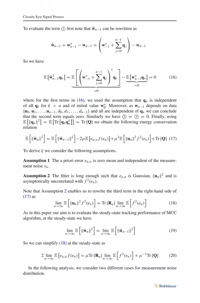
To evaluate the term 1© first note that w̃n−1 can be rewritten as

w̃n−1 = won−1 − wn−1 =

⎛⎝wo−1 +

n−1∑j=0

q j

⎞⎠ − wn−1

So we have

E[w̃Tn−1qn

] = E

⎡⎣

⎛⎝wo−1 +

n−1∑j=0

q j

⎞⎠

T

qn

⎤⎦

︸︷︷︸=0

−E[w∗n−1qn

]︸︷︷︸

=0

= 0 (16)

where for the first terms in (16), we used the assumption that qn is independentof all qk for k < n and of initial value wo

0. Moreover, as wn−1 depends on data{u0,u1, . . . ,un−1, d0, d1, . . . , dn−1} and all are independent of qn we can concludethat the second term equals zero. Similarly we have 2© = 3© = 0. Finally, usingE

[‖qn‖2] = E[Tr

[qnqT

n

]] = Tr [Q] we obtain the following energy conservationrelation

E

[‖w̃n‖2

]= E

[‖w̃n−1‖2

]−2μE

[ea,n f (en)

]+μ2E

[‖un‖2 f 2(en)

]+Tr [Q] (17)

To derive ξ we consider the following assumptions.

Assumption 1 The a priori error ea,n is zero mean and independent of the measure-ment noise vn .

Assumption 2 The filter is long enough such that ea,n is Gaussian, ‖un‖2 and isasymptotically uncorrelated with f 2(en).

Note that Assumption 2 enables us to rewrite the third term in the right-hand side of(17) as

limn→∞E

[‖un‖2 f 2(en)

]= Tr [Ru] lim

n→∞E

[f 2(en)

](18)

As in this paper our aim is to evaluate the steady-state tracking performance of MCCalgorithm, at the steady-state we have

limn→∞E

[‖w̃n‖2

]= lim

n→∞E

[‖w̃n−1‖2

](19)

So we can simplify (18) at the steady-state as

2 limn→∞E

[ea,n f (en)

] = μTr [Ru] limn→∞E

[f 2(en)

]+ μ−1Tr [Q] (20)

In the following analysis, we consider two different cases for measurement noisedistribution.


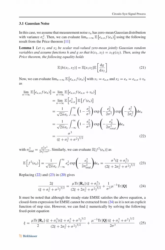
3.1 Gaussian Noise

In this case,we assume thatmeasurement noise vn has zero-meanGaussian distributionwith variance σ 2

v . Then, we can evaluate limn→∞ E[ea,n f (en)

]using the following

result from the Price theorem [11]

Lemma 1 Let x1 and x2 be scalar real-valued zero-mean jointly Gaussian randomvariables and assume functions h and g so that h(x1, x2) = x1g(x2). Then, using thePrice theorem, the following equality holds

E [h(x1, x2)] = E[x1x2]E[dg

dx2

](21)

Now, we can evaluate limn→∞ E[ea,n f (en)

]with x1 = ea,n and x2 = en = ea,n +vn

as

limn→∞E

[ea,n f (en)

] = limn→∞E

[ea,n f (ea,n + vn)

]

= limn→∞E

[e2a,n

]E

[f ′(en)

]

= 1√2πσe

∫ ∞

−∞

(1 − e2n

σ 2

)exp

(− e2n2σ 2

)exp

(− e2i2σ 2

e

)den

= 1√2πσe

∫ ∞

−∞

(1 − e2n

σ 2

)exp

(− e2n2σ 2

total

)den

= σ 3

(ξ + σ 2v + σ 2)

3/2 (22)

with σ 2total = σ 2

e σ 2

2σ 2e +σ 2 . Similarly, we can evaluate E[ f 2(en)] as

E

[f 2(en)

]= 1√

2πσe

∫ ∞

−∞e2n exp

(− e2n2σ 2

total

)den = σ 3(ξ + σ 2

v )

(2ξ + 2σ 2v + σ 2)

3/2 (23)

Replacing (22) and (23) in (20) gives

2ξ

(ξ + σ 2v + σ 2)

3/2 = μTr [Ru] (ξ + σ 2v )

(2ξ + 2σ 2v + σ 2)

3/2 + 1

σ 3μ−1Tr [Q] (24)

It must be noted that although the steady-state EMSE satisfies the above equation, aclosed-form expression for EMSE cannot be extracted from (24) as it is not an explicitfunction of step size. However, we can find ξ numerically by solving the followingfixed-point equation

ξ = μTr [Ru]

2

(ξ + σ 2v )(ξ + σ 2

v + σ 2)3/2

(2ξ + 2σ 2v + σ 2)

3/2 + μ−1Tr [Q] (ξ + σ 2v + σ 2)

3/2

2σ 3 (25)


Remark 1 As the kernel size σ → ∞, the EMSE value ξ given by (25) tends to theEMSE expression of the LMS algorithm, i.e.,

limσ→∞ ξ = μTr [Ru] σ 2

v + μ−1Tr [Q]

2 − μTr [Ru]= ξLMS (26)

3.2 Non-Gaussian Noise

To derive the theoretical expression for general non-Gaussian noise data, we consideragain the steady-state relation (20). Similar to the Gaussian noise case, we again needto evaluate E[ea,n f (en)] and E[ f 2(en)]. For the first moment, we have1

E[ea,n f (en)

] ≈ E[ea,n( f (vn) + f ′(vn)ea,n)

] ≈ ξE[ f ′(vn)] (27)

Similarly, for the second moment we have

E

[f 2(en)

]≈ E

[( f (vn) + f ′(vn)ea,n + 1

2f ′′(vn)e2a,n)

2]

≈ E

[f 2(vn)

]+ ξE

[f (vn) f

′′(vn) + ( f ′(vn))2]

(28)

The required terms f ′(vn) and f ′′(vn) are given by

f ′(vn) =(1 − v2n

σ 2

)exp

(−v2n

2σ 2

), f ′′(vn) =

(v3n

v4n− 3vn

σ 2

)exp

(−v2n

2σ 2

)(29)

Replacing (27) and (28) in (20) result in the desired EMSE expression for generalnoise distribution as follows

ξ =μTr [Ru]E

[v2n exp

(−v2nσ 2

)]+ μ−1Tr [Q]

2E[(

1 − v2nσ 2

)exp

(−v2n2σ 2

)]− μTr [Ru]E

[(1 + 2v4n

σ 4 − 5v2nσ 2

)exp

(−v2nσ 2

)] (30)

Remark 2 The given expression for EMSE in (30) is not an increasing monotonicfunction of μ. This can be easily verified by witting it as

ξ = μA + μ−1BC − μD (31)

1 We use the Taylor expansion of f (en) as f (en) = f (vn) + f ′(vn)ea,n + 12 f ′′(vn)e2a,n + o(e2a,n).


with

A = Tr [Ru]E

[v2n exp

(−v2n

σ 2

)](32a)

B = Tr [Q] (32b)

C = 2E

[(1 − v2n

σ 2

)exp

(−v2n

2σ 2

)](32c)

D = Tr [Ru]E

[(1 + 2v4n

σ 4 − 5v2nσ 2

)exp

(−v2n

σ 2

)](32d)

By setting the first derivative of the above equation to zero (i.e., dξdμ = 0), we obtain

the following equationACμ2 + 2BD − BC = 0 (33)

The optimum step size for which the ξ takes its minimum is the positive root of (33).

4 Simulation Results

In this section, we provide the simulation results in order to verify the theoreticalanalysis. To this end, we consider a system identification setup which involves deter-mining the coefficients of an unknown filter with length M = 10. The input vectorun is generated from a Gaussian process with covariance matrix R = I. For the non-stationary environment, we assume a randomwalk model withQ = 10−4Iwith initialvector w0 = 0. We use a Gaussian kernel with size σ = 2. The steady-state EMSEcurves are generated by performing the MCC algorithm for 10,000 iterations and thenaveraging the last 200 samples.

For the Gaussian case, we assume that measurement noise in (1) is zero-meanGaussian noise with variance σ 2

v = 0.1. The steady-state curve for Gaussian caseis shown in Fig. 1. We can observe that the simulation result matches well with thetheoretical expression given by the Eq. (25). We can also see that the EMSE curveis not monotonic increasing function of step size parameter. It is worth noting thatsimilar to LMS algorithm, the requirement of step size for convergence rate, time-varying tracking accuracy and convergence precision (steady-state performance) iscontradictory. When μ is too small, convergence rate is slow and the MCC algorithmcannot track the optimal weight variations, which, in turn, results in large steady-stateEMSE. Increasing μ improves convergence rate and tracking accuracy and reducesthe steady-state EMSE. Finally, as μ increases further, oscillation occurs during theconvergence and the steady-state performance deteriorates again.

Note further that for this case an optimum step size value cannot be obtained from(25) as it is not an explicit function of step size.

For the Gaussian case, we consider two different distributions for measurementnoise including (1) uniform distribution, where the uniform noise is distributed over[−1 + 1], and (2) exponential distribution with mean parameter λ = 2. The othersimulation parameters remain unchanged. Figure 2 shows the EMSE curves for both


0 0.01 0.02 0.03 0.04 0.05 0.06 0.07 0.08−15

−14

−13

−12

−11

−10

−9

−8

μ

ξ (

dB)

SimulationTheory

Fig. 1 Comparing theoretical and simulation EMSE for Gaussian noise: uniform distribution (left), expo-nential distribution (right)

0.01 0.02 0.03 0.04 0.05 0.06−7

−6

−5

−4

−3

−2

−1

μ

ξ (d

B)

0 0.01 0.02 0.03 0.04 0.05 0.06−12

−11

−10

−9

−8

−7

−6

−5

μ

ξ (d

B)

SimulationTheory

SimulationTheory

μmin

=0.0123

μmin

=0.0175

Fig. 2 Comparing theoretical and simulation EMSE for non-Gaussian noise

of the non-Gaussian noise distributions. As it is seen from Fig. 2, the EMSE obtainedfrom the simulation nicely fits the theoretical result obtained earlier. Moreover, forboth cases the optimum values given by (33) are very close to the optimum valuesgiven by simulations.

5 Conclusions

In this paper, we studied the tracking analysis of MCC algorithm, when the optimumweight vector varies according to a random walk model. Our analysis, which relieson the energy conservation approach revealed that, independent of the measurementnoise model, the EMSE curve is not an increasing function of step size parameter.Therefore, in non-stationary environments it is vital to select an appropriate step sizeto achieve an acceptable performance. The simulation results were in good agreementwith the analysis.


References

1. W. Bazzi, A. Rastegarnia, A. Khalili, A robust diffusion adaptive network based on the maximumcorrentropy criterion, in Computer Communication and Networks (ICCCN), 2015 24th InternationalConference on, pp. 1–4 (2015)

2. B. Chen, J. Wang, H. Zhao, N. Zheng, J. Principe, Convergence of a fixed-point algorithm undermaximum correntropy criterion. Signal Process. Lett. IEEE 22(10), 1723–1727 (2015)

3. B. Chen, L. Xing, J. Liang, N. Zheng, J. Principe, Steady-state mean-square error analysis for adaptivefiltering under the maximum correntropy criterion. Signal Process. Lett. IEEE 21(7), 880–884 (2014)

4. B. Chen, J. Wang, H. Zhao, N. Zheng, J. Principe, Convergence of a fixed-point algorithm undermaximum correntropy criterion. Signal Process. Lett. IEEE 22(10), 1723–1727 (2015)

5. D. Erdogmus, Information theoretic learning: Renyi’s entropy and its applications to adaptive systemtraining. Ph.D. dissertation, University of Florida (2002)

6. D. Erdogmus, J.C. Principe, Generalized information potential criterion for adaptive system training.IEEE Trans. Neural Netw. 13(5), 1035–1044 (2002)

7. S. Han, A family of minimum Renyi’s error entropy algorithm for information processing. Ph.D.dissertation, University of Florida (2007)

8. S. Haykin, Adaptive Filter Theory, 3rd edn. (Prentice-Hall, Upper Saddle River, NJ, 1996)9. A. Khalili, A. Rastegarnia, S. Sanei, Robust frequency estimation in three-phase power systems using

correntropy-based adaptive filter. Sci. Meas. Technol. IET 9(8), 928–935 (2015)10. W. Liu, P.P. Pokharel, J.C. Principe, Correntropy: properties, and applications in non-gaussian signal

processing. IEEE Trans. Signal Process. 55(11), 5286–5298 (2007)11. R. Price, A useful theorem for nonlinear devices having gaussian inputs. Inf. Theory, IRE Trans. 4(2),

69–72 (1958)12. J.C. Principe, Information Theoretic Learning: Renyi’s Entropy and Kernel Perspectives (Springer,

Berlin, 2010)13. L. Shi, Y. Lin, Convex combination of adaptive filters under the maximum correntropy criterion in

impulsive interference. Signal Process. Lett. IEEE 21(11), 1385–1388 (2014)14. A. Singh, J. Principe, Using correntropy as a cost function in linear adaptive filters, inNeural Networks,

2009. IJCNN 2009. International Joint Conference on, pp. 2950–2955 (2009)15. R. Wang, B. Chen, N. Zheng, J. Principe, A variable step-size adaptive algorithm under maximum

correntropy criterion, in Neural Networks (IJCNN), 2015 International Joint Conference on, pp. 1–5(2015)

16. B. Widrow, M. Hoff, Adaptive switching circuits. IRE WESCON Conv. Rec. 4, 96–104 (1960)17. S. Zhao, B. Chen, J.C. Principe, Kernel adaptive filtering with maximum correntropy criterion, in

International Joint Conference on Neural Networks (IJCNN), pp. 2012–2017 (2011)

Documents

Steady-State Tracking Analysis of Adaptive Filter With Maximum Correntropy Criterion