arX

iv:p

hysi

cs/0

6070

43v2

[ph

ysic

s.op

tics]

29

Jan

2007

Statistical analysis of time-resolved emission from ensembles of

semiconductor quantum dots: interpretation of exponential decay

models

A. F. van Driel,1 I. S. Nikolaev,2, 3 P. Vergeer,1 P.

Lodahl,3, 4 D. Vanmaekelbergh,1 and W. L. Vos2, 3, ∗

1Debye Institute, Utrecht University,

P.O. Box 80 000, 3508 TA Utrecht, The Netherlands

2Center for Nanophotonics, FOM Institute for Atomic and Molecular Physics (AMOLF),

1098 SJ Amsterdam, The Netherlands

3Complex Photonic Systems (COPS),

Department of Science and Technology and MESA+ Research Institute,

University of Twente, 7500 AE Enschede, The Netherlands

4COM·DTU Department of Communications, Optics, and Materials,

Nano·DTU, Technical University of Denmark, Denmark

(Dated: Prepared for Phys. Rev. B in October, 2006.)

1

Abstract

We present a statistical analysis of time-resolved spontaneous emission decay curves from en-

sembles of emitters, such as semiconductor quantum dots, with the aim to interpret ubiquitous

non-single-exponential decay. Contrary to what is widely assumed, the density of excited emitters

and the intensity in an emission decay curve are not proportional, but the density is a time-integral

of the intensity. The integral relation is crucial to correctly interpret non-single-exponential decay.

We derive the proper normalization for both a discrete, and a continuous distribution of rates,

where every decay component is multiplied with its radiative decay rate. A central result of our

paper is the derivation of the emission decay curve in case that both radiative and non-radiative

decays are independently distributed. In this case, the well-known emission quantum efficiency can

not be expressed by a single number anymore, but it is also distributed. We derive a practical de-

scription of non-single-exponential emission decay curves in terms of a single distribution of decay

rates; the resulting distribution is identified as the distribution of total decay rates weighted with

the radiative rates. We apply our analysis to recent examples of colloidal quantum dot emission

in suspensions and in photonic crystals, and we find that this important class of emitters is well

described by a log-normal distribution of decay rates with a narrow and a broad distribution, re-

spectively. Finally, we briefly discuss the Kohlrausch stretched-exponential model, and find that

its normalization is ill-defined for emitters with a realistic quantum efficiency of less than 100 %.

2

X*

X

heat

concentration c( t )

intensity f

Grad Gnradhn

intensity g-f

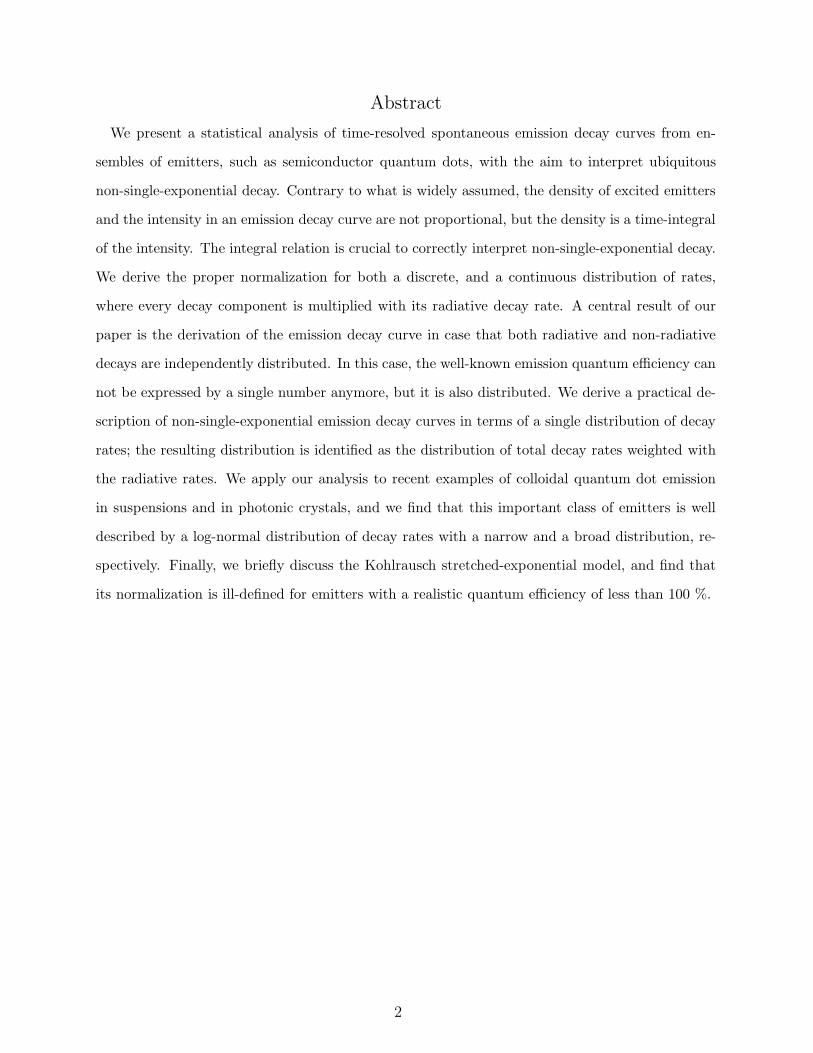
FIG. 1: Schematic of the relation between decay of an excited state X∗ to the ground state X and

experimental observable parameters. The density of emitters in the excited state is equal to c(t)

which can be probed by transient absorption. The emitted light intensity as a function of time

f(t) is recorded in luminescence decay measurements. In photothermal measurements the released

heat (g− f)(t) after photoexcitation is detected. g(t) describes the total decay, i.e., the sum of the

radiative and the non-radiative decay.

I. INTRODUCTION

Understanding the decay dynamics of excited states in emitters such as semiconductor

quantum dots is of key importance for getting insight in many physical, chemical and biolog-

ical processes. For example, in biophysics the influence of Forster resonance energy transfer

on the decay dynamics of donor molecules is studied to quantify molecular dynamics1,2.

In cavity quantum electrodynamics, modification of the density of optical modes (DOS) is

quantified by measuring the decay dynamics of light sources. According to Fermi’s ’Golden

Rule’ the radiative decay rate is proportional to the DOS at the location of the emitter3.

Nanocrystalline quantum dots2,4,5, atoms6,7 and dye molecules8,9 are used as light sources

in a wide variety of systems. Examples of such systems are many different kinds of pho-

tonic materials, including metallic and dielectric mirrors5,6,7,8,9, cavities10, metallic films11,12,

two13,14-, and three-dimensional15 photonic crystals.

3

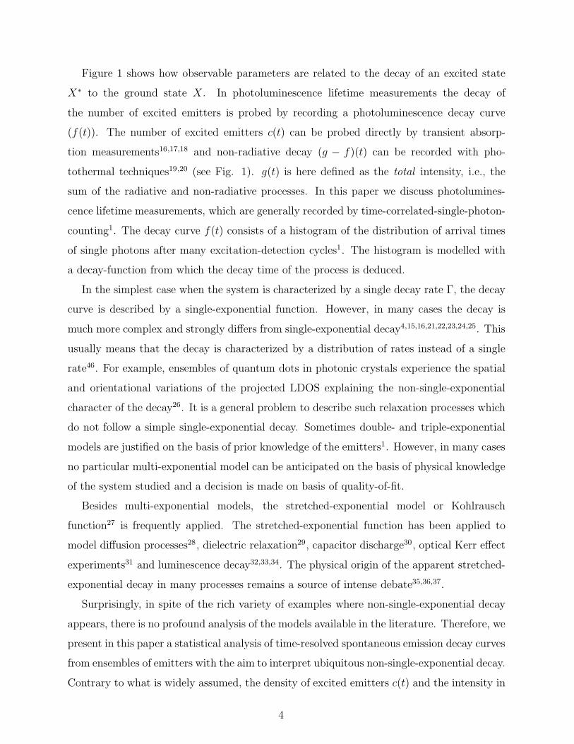
Figure 1 shows how observable parameters are related to the decay of an excited state

X∗ to the ground state X. In photoluminescence lifetime measurements the decay of

the number of excited emitters is probed by recording a photoluminescence decay curve

(f(t)). The number of excited emitters c(t) can be probed directly by transient absorp-

tion measurements16,17,18 and non-radiative decay (g − f)(t) can be recorded with pho-

tothermal techniques19,20 (see Fig. 1). g(t) is here defined as the total intensity, i.e., the

sum of the radiative and non-radiative processes. In this paper we discuss photolumines-

cence lifetime measurements, which are generally recorded by time-correlated-single-photon-

counting1. The decay curve f(t) consists of a histogram of the distribution of arrival times

of single photons after many excitation-detection cycles1. The histogram is modelled with

a decay-function from which the decay time of the process is deduced.

In the simplest case when the system is characterized by a single decay rate Γ, the decay

curve is described by a single-exponential function. However, in many cases the decay is

much more complex and strongly differs from single-exponential decay4,15,16,21,22,23,24,25. This

usually means that the decay is characterized by a distribution of rates instead of a single

rate46. For example, ensembles of quantum dots in photonic crystals experience the spatial

and orientational variations of the projected LDOS explaining the non-single-exponential

character of the decay26. It is a general problem to describe such relaxation processes which

do not follow a simple single-exponential decay. Sometimes double- and triple-exponential

models are justified on the basis of prior knowledge of the emitters1. However, in many cases

no particular multi-exponential model can be anticipated on the basis of physical knowledge

of the system studied and a decision is made on basis of quality-of-fit.

Besides multi-exponential models, the stretched-exponential model or Kohlrausch

function27 is frequently applied. The stretched-exponential function has been applied to

model diffusion processes28, dielectric relaxation29, capacitor discharge30, optical Kerr effect

experiments31 and luminescence decay32,33,34. The physical origin of the apparent stretched-

exponential decay in many processes remains a source of intense debate35,36,37.

Surprisingly, in spite of the rich variety of examples where non-single-exponential decay

appears, there is no profound analysis of the models available in the literature. Therefore, we

present in this paper a statistical analysis of time-resolved spontaneous emission decay curves

from ensembles of emitters with the aim to interpret ubiquitous non-single-exponential decay.

Contrary to what is widely assumed, the density of excited emitters c(t) and the intensity in

4

an emission decay curve (f(t) or g(t)) are not proportional, but the density is a time-integral

of the intensity. The integral relation is crucial to correctly interpret non-single-exponential

decay. We derive the proper normalization for both a discrete, and a continuous distribution

of rates, where every decay component is multiplied with its radiative decay rate. A central

result of our paper is the derivation of the emission decay curve f(t) in case that both

radiative and non-radiative decays are independently distributed. In this most general case,

the well-known emission quantum efficiency is also distributed. Distributed radiative decay

is encountered in photonic media26, while distributed non-radiative decay has been reported

for colloidal quantum dots32,34 and powders doped with rare-earths38. We derive a practical

description of non-single-exponential emission decay curves in terms of the distribution of

total decay rates weighted with the radiative rates. Analyzing decay curves in terms of

distributions of decay rates has the advantage that information on physically interpretable

rates is readily available, as opposed to previously reported analysis in terms of lifetimes. We

apply our analysis to recent examples of colloidal quantum dot emission in suspensions and

in photonic crystals. We find excellent agreement with a log-normal distribution of decay

rates for such quantum dots. In the final Section, we discuss the Kohlrausch stretched-

exponential model, and find that its normalization is ill-defined for emitters with a realistic

quantum efficiency of less than 100 %.

II. DECAY MODELS

A. Relation between the concentration of emitters and the decay curve

A decay curve is the probability density of emission which is therefore modelled with a

so-called probability density function39. This function tends to zero in the limit t → ∞.

The decay of the fraction of excited emitters c(t′

)c(0)

at time t′ is described with a reliability

function or cumulative distribution function(

1 − c(t′

)c(0)

)

39. Here c(0) is the concentration of

excited emitters at t′ = 0. The reliability function tends to one in the limit t′

→ ∞ and

to zero in the limit t′

→ 0. The fraction of excited emitters and the decay curve, i.e., the

reliability function and the probability density function39, are related as follows:

∫ t′

0g(t)dt = 1 −

c(t′

)

c(0)(1)

5

0 2 4 6 8 1010-2

10-1

100

101

10-2

10-1

100

101

g(t)c(

t)/c(

0)

t (units of Gstr-1)

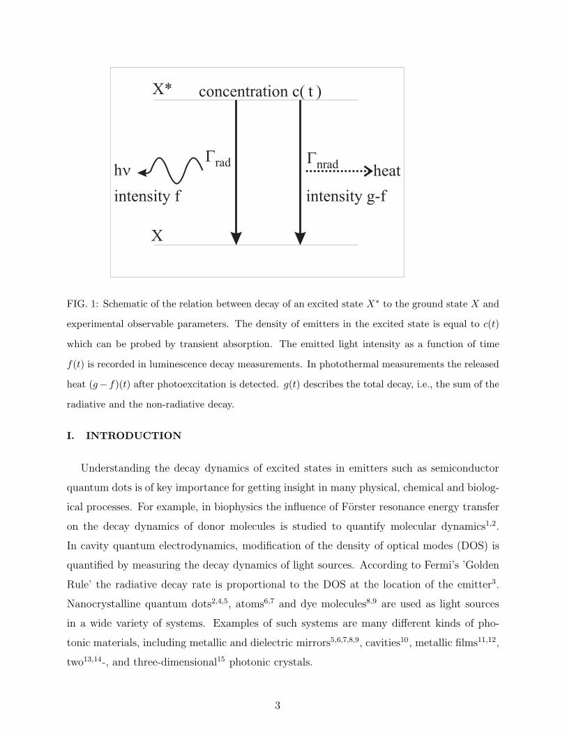
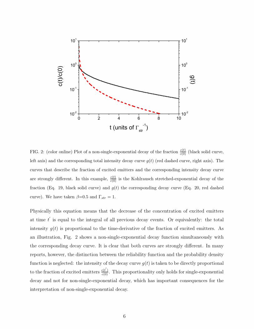
FIG. 2: (color online) Plot of a non-single-exponential decay of the fraction c(t)c(0) (black solid curve,

left axis) and the corresponding total intensity decay curve g(t) (red dashed curve, right axis). The

curves that describe the fraction of excited emitters and the corresponding intensity decay curve

are strongly different. In this example, c(t)c(0) is the Kohlrausch stretched-exponential decay of the

fraction (Eq. 19, black solid curve) and g(t) the corresponding decay curve (Eq. 20, red dashed

curve). We have taken β=0.5 and Γstr = 1.

Physically this equation means that the decrease of the concentration of excited emitters

at time t′

is equal to the integral of all previous decay events. Or equivalently: the total

intensity g(t) is proportional to the time-derivative of the fraction of excited emitters. As

an illustration, Fig. 2 shows a non-single-exponential decay function simultaneously with

the corresponding decay curve. It is clear that both curves are strongly different. In many

reports, however, the distinction between the reliability function and the probability density

function is neglected: the intensity of the decay curve g(t) is taken to be directly proportional

to the fraction of excited emitters c(t′

)c(0)

. This proportionality only holds for single-exponential

decay and not for non-single-exponential decay, which has important consequences for the

interpretation of non-single-exponential decay.

6

0 50 100 150 200 250100

101

102

103

10-3

10-2

10-1

100

normalized f(t)

Inte

nsity

(cou

nts)

t (ns)

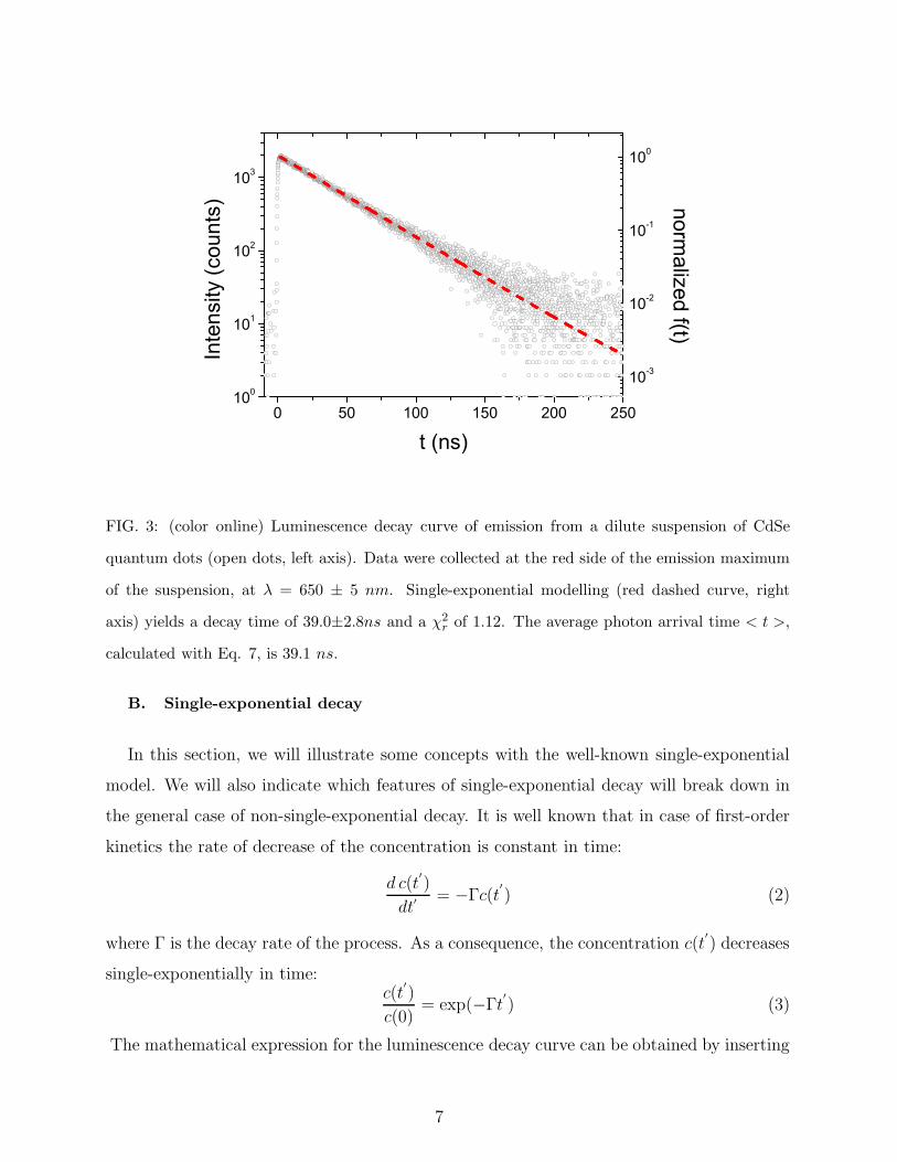
FIG. 3: (color online) Luminescence decay curve of emission from a dilute suspension of CdSe

quantum dots (open dots, left axis). Data were collected at the red side of the emission maximum

of the suspension, at λ = 650 ± 5 nm. Single-exponential modelling (red dashed curve, right

axis) yields a decay time of 39.0±2.8ns and a χ2r of 1.12. The average photon arrival time < t >,

calculated with Eq. 7, is 39.1 ns.

B. Single-exponential decay

In this section, we will illustrate some concepts with the well-known single-exponential

model. We will also indicate which features of single-exponential decay will break down in

the general case of non-single-exponential decay. It is well known that in case of first-order

kinetics the rate of decrease of the concentration is constant in time:

d c(t′

)

dt′

= −Γc(t′

) (2)

where Γ is the decay rate of the process. As a consequence, the concentration c(t′

) decreases

single-exponentially in time:c(t

′

)

c(0)= exp(−Γt

′

) (3)

The mathematical expression for the luminescence decay curve can be obtained by inserting

7

Eq. 3 into Eq. 1, where Γ is identified with the total decay rate Γtot, resulting in:

g(t) = Γrad exp(−Γtott) + Γnrad exp(−Γtott) (4)

where Γrad is the radiative decay rate, Γnrad is the nonradiative decay rate and Γtot is the

total decay rate with Γtot = Γrad + Γnrad. In a luminescence decay measurement the recorded

signal is proportional to the first term of g(t) only which is f(t):

f(t) = αΓrad exp(−Γtott) (5)

and therefore a single-exponential luminescence decay process is modelled with Eq. 5. The

pre-exponential factor α is usually taken as adjustable parameter, and it is related to several

experimental parameters, i.e., the number of excitation-emission cycles in the experiment,

the photon-collection efficiency and the concentration of the emitter. Henceforth α will be

omitted in our analysis. A comparison between Eqs. 5 and 3 shows that in the case of pure

single-exponential decay neglect of the distinction between the reliability function (Eq. 3)

and the probability density function (Eq. 5) has no important consequences, since both the

fraction and the decay curve are single-exponential. As Fig. 2 shows, this neglect breaks

down in the case of non-single-exponential decay.

Figure 3 shows a luminescence decay curve of a dilute suspension of CdSe quantum dots

in chloroform at a wavelength of λ = 650 ± 5 nm40, with the number of counts on the

ordinate and the time on the abscissa. Clearly, the data agree well with single-exponential

decay as indicated by the quality-of-fit χ2r of 1.12, close to the ideal value of 1. This means

that all individual quantum dots that emit light in this particular wavelength-range do so

with the same rate of 139.0

ns−1. It appears that the rate of emission strongly depends on the

emission frequency and that it is determined by the properties of the bulk semiconductor

crystal40.

Since f(t) as given by Eq. 5 is a probability density function, the probability of emission

in a certain time-interval can be deduced by integration. The total probability for emission

at all times between t = 0 and t → ∞ is given by∫

∞

0f(t)dt =

∫

∞

0Γrad exp(−Γtott)dt =

Γrad

Γtot

(6)

which is equal to the luminescence quantum efficiency. The luminescence quantum efficiency

is defined as the probability of emission after excitation1. The correct recovery of this result

in Eq. 6 shows that Eq. 5 is properly normalized.

8

The average arrival time of the emitted photons or the average decay time can be calcu-

lated by taking the first moment of Eq. 5:

< t >= τav =

∫

∞

0 f(t)tdt∫

∞

0 f(t)dt=

1

Γtot

(7)

Only in the case of single-exponential decay the average decay time < t > is equal to the

inverse of the total decay rate Γtot. The average arrival time for the data in Fig. 3 was

< t >= 39.1 ns, very close to the value of 39.0 ±2.8ns obtained from single-exponential

modelling, which further confirms the single-exponential character of the decay of quantum

dots in suspension.

C. Discrete distribution of decay rates

In contrast to the example shown in Fig. 3, there are many cases in which decay curves

cannot be modelled with a single-exponential function. As an example, Fig. 4 shows a

strongly non-single-exponential decay curve of spontaneous emission from CdSe quantum

dots in an inverse opal photonic crystal15,26. If a non-single-exponential decay curve is

modelled with a sum of single-exponentials, the decay curve has the following form:

f(t) =1

c(0)

n∑

i=1

ciΓrad,i exp(−Γtot,it) (8)

where n is the number of different emitters (or alternatively the number of different envi-

ronments of single emitters26), ci is the concentration of emitters that has a radiative decay

rate Γrad,i, and c(0) is the concentration of excited emitters at t = 0, i.e., the sum of all con-

centrations ci. When the different fractions (or environments) are distributed in a particular

way, a distribution function ρ(Γtot) may be used. Such a function describes the distribution

or concentration of the emitters over the emission decay rates at time t = 0. The fraction

of emitters with a total decay rate Γtot,i is equal to

ci

c(0)=

1

c(0)

(c(Γtot,i−1) + c(Γtot,i+1))

2(9)

=1

2

∫ Γtot,i+1

Γtot,i−1

ρ(Γtot)dΓtot

= ρ(Γtot,i)∆Γtot

where ρ(Γtot,i) expresses the distribution of the various components i over the rates Γtot,i

and has units of inverse rate s. ∆Γtot is the separation between the various components i in

9

0 20 40 60 80

102

103

104

102

103

104

10-2

10-1

100

10-2

10-1

100 normalized f(t)

Inte

nsity

(cou

nts) norm

alized g(t)In

tens

ity (c

ount

s)

t (ns)

(b)

(a)

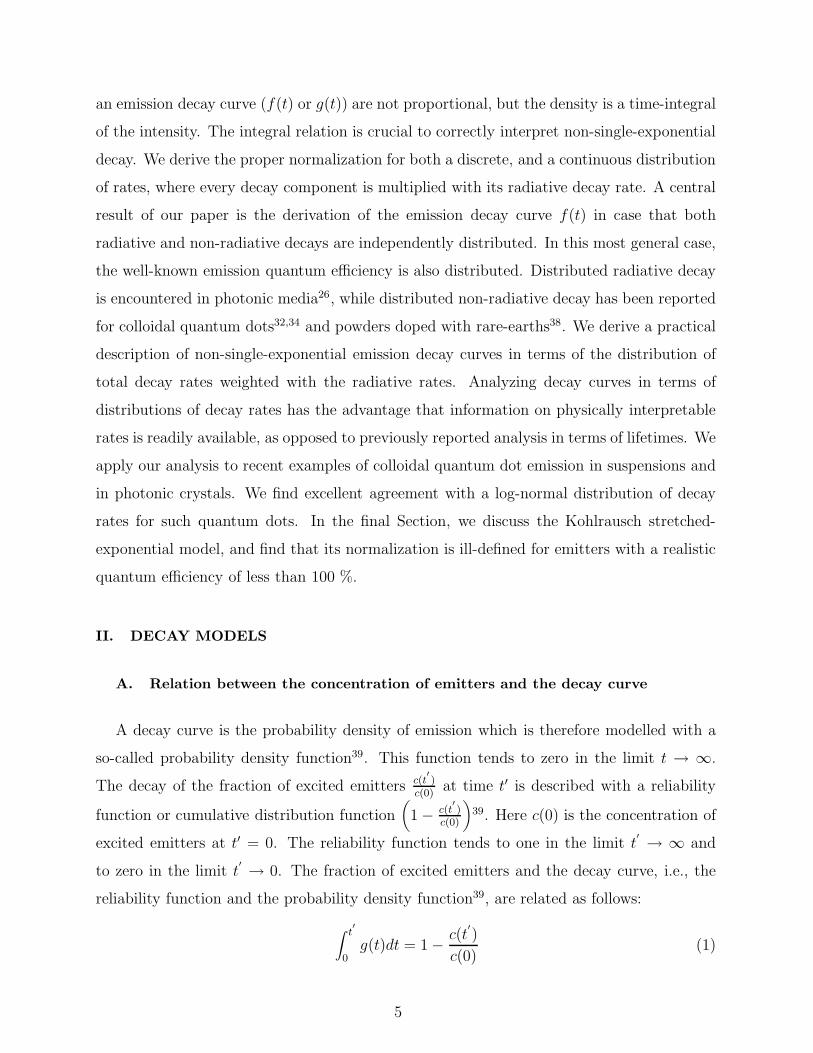
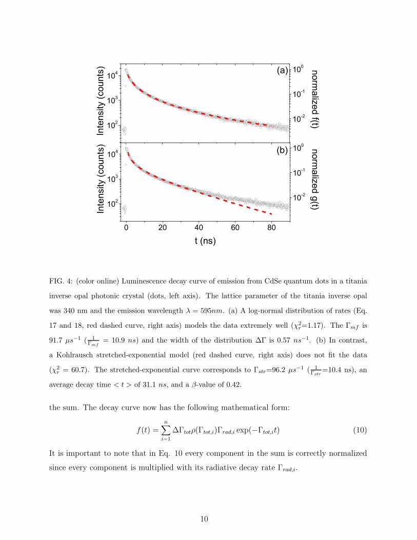
FIG. 4: (color online) Luminescence decay curve of emission from CdSe quantum dots in a titania

inverse opal photonic crystal (dots, left axis). The lattice parameter of the titania inverse opal

was 340 nm and the emission wavelength λ = 595nm. (a) A log-normal distribution of rates (Eq.

17 and 18, red dashed curve, right axis) models the data extremely well (χ2r=1.17). The Γmf is

91.7 µs−1 ( 1Γmf

= 10.9 ns) and the width of the distribution ∆Γ is 0.57 ns−1. (b) In contrast,

a Kohlrausch stretched-exponential model (red dashed curve, right axis) does not fit the data

(χ2r = 60.7). The stretched-exponential curve corresponds to Γstr=96.2 µs−1 ( 1

Γstr=10.4 ns), an

average decay time < t > of 31.1 ns, and a β-value of 0.42.

the sum. The decay curve now has the following mathematical form:

f(t) =n

∑

i=1

∆Γtotρ(Γtot,i)Γrad,i exp(−Γtot,it) (10)

It is important to note that in Eq. 10 every component in the sum is correctly normalized

since every component is multiplied with its radiative decay rate Γrad,i.

10

D. Continuous distribution of decay rates

For infinitesimal values of ∆Γtot, Eq. 10 can be written as an integral:

f(t) =∫

∞

0Γrad(Γtot)ρ(Γtot) exp(−Γtott)dΓtot (11)

In the case of single-exponential decay the distribution function is strongly peaked around a

central Γtot-value, i.e., the distribution function is a Dirac delta function. Inserting a Dirac

delta function into Eq. 11 recovers Eq. 5:

f(t) =∫

∞

0Γrad′ δ(Γtot − Γtot′) exp(−Γtott)dΓtot

= Γrad′ exp(−Γtot′t) (12)

This result confirms that the generalization to Eq. 11 is correct since it yields the correctly

normalized single-exponential functions.

In Eq. 11 it is tacitly assumed that for every Γtot there is one Γrad: the function Γrad(Γtot)

relates each Γtot to exactly one Γrad. In general both Γtot and Γrad vary independently, and

Eq. 11 is generalized to

f(t) (13)

=∫

∞

0

[

∫ Γtot

0dΓrad ρΓtot

(Γrad) Γrad

]

ρ(Γtot) exp(−Γtott)dΓtot

where ρΓtot(Γrad) is the normalized distribution of Γrad at constant Γtot. For every Γtot

the integration is performed over all radiative rates; a distribution of Γrad is taken into

account for every Γtot. Eq. 13 is the most general expression of a luminescence decay curve

and a central result of our paper. From this equation every decay curve with a particular

distribution of rates can be recovered. An example described by Eq. 13 is an ensemble of

quantum dots in a photonic crystal. In photonic crystals the local density of optical states

(LDOS) varies with the location in the crystal and the distribution of dipole orientations

of the emitters41. Therefore, an ensemble of emitters with a certain frequency emit light

with a distribution of radiative rates Γrad. In addition, when an ensemble of emitters has

a distributed Γtot and a single radiative rate Γrad, i.e., ρΓtot(Γrad) is a delta-function, then

Eq. 13 reduces to Eq. 11. Even though the non-radiative rates may still be distributed,

Eq. 11 suffices to describe the decay curve since for every Γtot there is only one Γrad. Such a

situation appears, for example, with powders doped with rare earth ions38 and with polymer

films doped with quantum dots32,34.

11

10-3 10-2 10-1 100 101

(b)

(a)

DG

Gmf

s

G (ns-1)

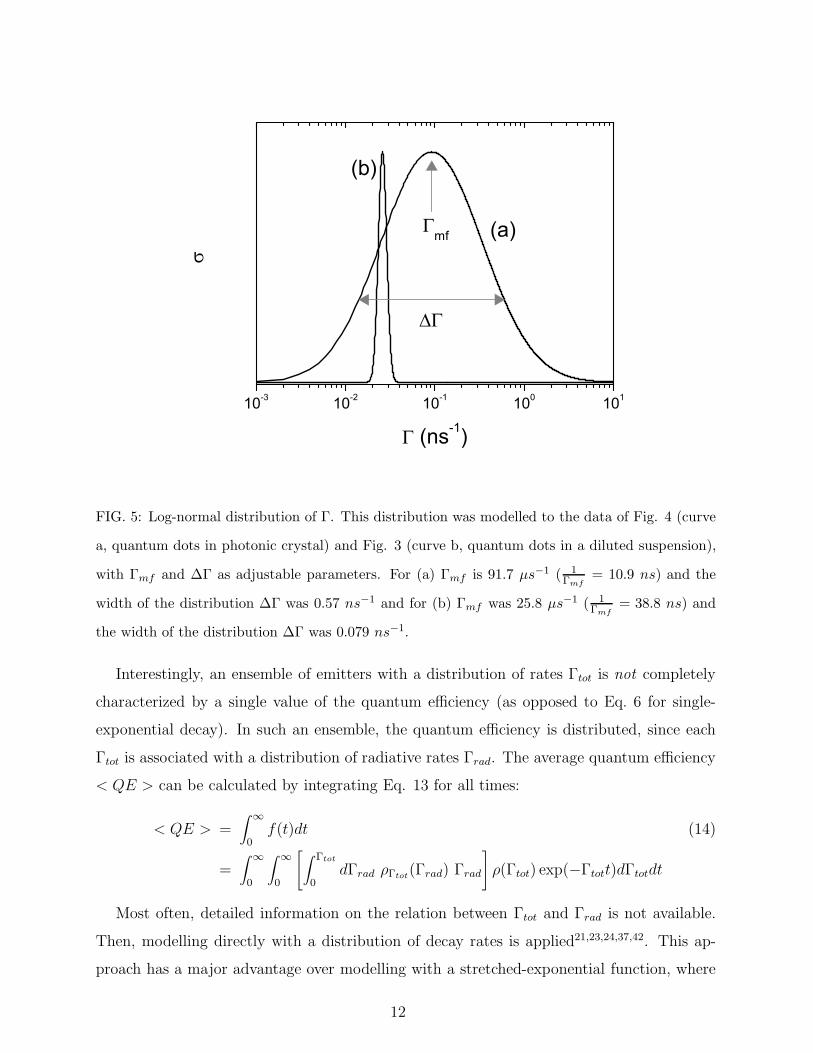
FIG. 5: Log-normal distribution of Γ. This distribution was modelled to the data of Fig. 4 (curve

a, quantum dots in photonic crystal) and Fig. 3 (curve b, quantum dots in a diluted suspension),

with Γmf and ∆Γ as adjustable parameters. For (a) Γmf is 91.7 µs−1 ( 1Γmf

= 10.9 ns) and the

width of the distribution ∆Γ was 0.57 ns−1 and for (b) Γmf was 25.8 µs−1 ( 1Γmf

= 38.8 ns) and

the width of the distribution ∆Γ was 0.079 ns−1.

Interestingly, an ensemble of emitters with a distribution of rates Γtot is not completely

characterized by a single value of the quantum efficiency (as opposed to Eq. 6 for single-

exponential decay). In such an ensemble, the quantum efficiency is distributed, since each

Γtot is associated with a distribution of radiative rates Γrad. The average quantum efficiency

< QE > can be calculated by integrating Eq. 13 for all times:

< QE > =∫

∞

0f(t)dt (14)

=∫

∞

0

∫

∞

0

[

∫ Γtot

0dΓrad ρΓtot

(Γrad) Γrad

]

ρ(Γtot) exp(−Γtott)dΓtotdt

Most often, detailed information on the relation between Γtot and Γrad is not available.

Then, modelling directly with a distribution of decay rates is applied21,23,24,37,42. This ap-

proach has a major advantage over modelling with a stretched-exponential function, where

12

it is complicated to deduce the distribution of decay rates (see below). A function of the

following form is used to model the non-single-exponential decay curve:

f(t) =∫

∞

0σ(Γtot) exp(−Γtott)dΓtot (15)

In Eq. 15 the various components are not separately normalized as in Eq. 13. Modelling

with Eq. 15 boils down to using an infinite series of single-exponentials which are expressed

with only a few free parameters. The form of the distribution can usually not be predicted

and a decision is made on basis of quality-of-fit. While a good fit does not prove that the

chosen distribution is unique, it does extract direct physical information from the non-single-

exponential decay on an ensemble of emitters and their environment26.

It is widely assumed that σ(Γ) is equal to the distribution of total rates21,23,24,43,44. A com-

parison with Eq. 13 shows that this is not true and reveals that σ(Γ) contains information

about both the radiative and non-radiative rates:

σ(Γtot) = ρ(Γtot)∫ Γtot

0ρΓtot

(Γrad) ΓraddΓrad (16)

Thus σ(Γ) is the distribution of total decay rates weighted by the radiative rates. This

conclusion demonstrates the practical use of Eq. 13: the equation allows us to completely

interpret the distribution of rates found by modelling with Eq. 15. Such a complete inter-

pretation has not been reported before.

E. Log-normal distribution of decay rates

Distribution functions that can be used for σ(Γ) are (sums of) normal, Lorentzian, and

log-normal distribution functions. In Fig. 4(a) the luminescence decay curve of quantum

dots is successfully modelled with Eq. 15, with a log-normal distribution of the rate Γ

σ(Γ) = A exp

[

−(ln Γ − ln Γmf

γ)2

]

(17)

where A is the normalization constant, Γmf is the most frequent rate constant (see Fig. 5).

γ is related to the width of the distribution:

∆Γ = 2Γmf sinh(γ) (18)

where ∆Γ is equal to the width of the distribution at 1e. The most frequent rate constant Γmf

and γ are adjustable parameters, only one extra adjustable parameter compared to a single-

exponential model. Clearly, this model (Eq. 15 and 17) describes our non-single-exponential

13

experimental data extremely well. The χ2r was 1.17, Γmf was 91.7 µs−1 ( 1

Γmf= 10.9 ns) and

the width of the distribution ∆Γ was 0.57 ns−1. In addition to Γmf and ∆Γ, an average

decay rate can be deduced from the log-normal distribution in Fig. 5 . However, this average

is biased since the various components are weighted with their quantum efficiency, as shown

in Eq. 16.

Modelling with a log-normal distribution of decay rates yields direct and clear physical

parameters, for instance the shape and width of the decay rate distribution. The log-normal

function is plotted in Fig. 5 (curve a). The broad distribution of rates demonstrates the

strongly non-single-exponential character of the decay curve. In Ref. 26 we were able to

relate the width of this broad distribution to the spatial and orientational variations of the

LDOS in inverse-opal photonic crystals.

The log-normal model was also modelled to the decay curve from quantum dots in sus-

pension (Fig. 3). The distribution is plotted in Fig. 5 (curve b). Γmf was 25.8 µs−1

( 1Γmf

= 38.8 ns), close to the lifetime deduced from the single-exponential modelling of 39.0

±2.8ns. The narrow width of the distribution ∆Γ of 0.079 ns−1 is in agreement with the

single-exponential character of the decay curve.

F. Stretched-exponential decay

Besides the multi-exponential models discussed in Sections C-E, the Kohlrausch

stretched-exponential decay model27,29 is widely applied to model non-single-exponential de-

cay curves. The fraction of excited emitters, i.e., the reliability function, of the Kohlrausch

stretched-exponential model is equal to:

c(t′

)

c(0)= exp(−(Γstrt

′

)β) (19)

where β is the stretch parameter, which varies between 0 and 1, and Γstr the total decay

rate in case of stretched-exponential decay. The stretch parameter β qualitatively expresses

the underlying distribution of rates: a small β means that the distribution of rates is broad

and β close to 1 implies a narrow distribution. The recovery of the distribution of rates in

case of stretched-exponential decay is mathematically complicated47 and only feasible for

specific β’s22,29,35,36.

The decay curve corresponding to a Kohlrausch stretched-exponential decay of the frac-

14

tion c(t′

)c(0)

can be deduced using Eq. 19 and Eq. 1, and results in:

g(t) =β

t(Γstrt)

β exp(−(Γstrt)β) (20)

The normalization of Eq. 20 can, in analogy with Eq. 6, be deduced by integration for all

times between t = 0 and t → ∞, which yields 1. Therefore, an important consequence is

that Eq. 20 is correctly normalized only for emitters with a quantum yield of 1 (Γrad = Γtot

and f(t) = g(t)). It is not clear how normalization should be done in realistic cases with

quantum yield < 100%. To the best of our knowledge, this problem has been overlooked in

the literature.

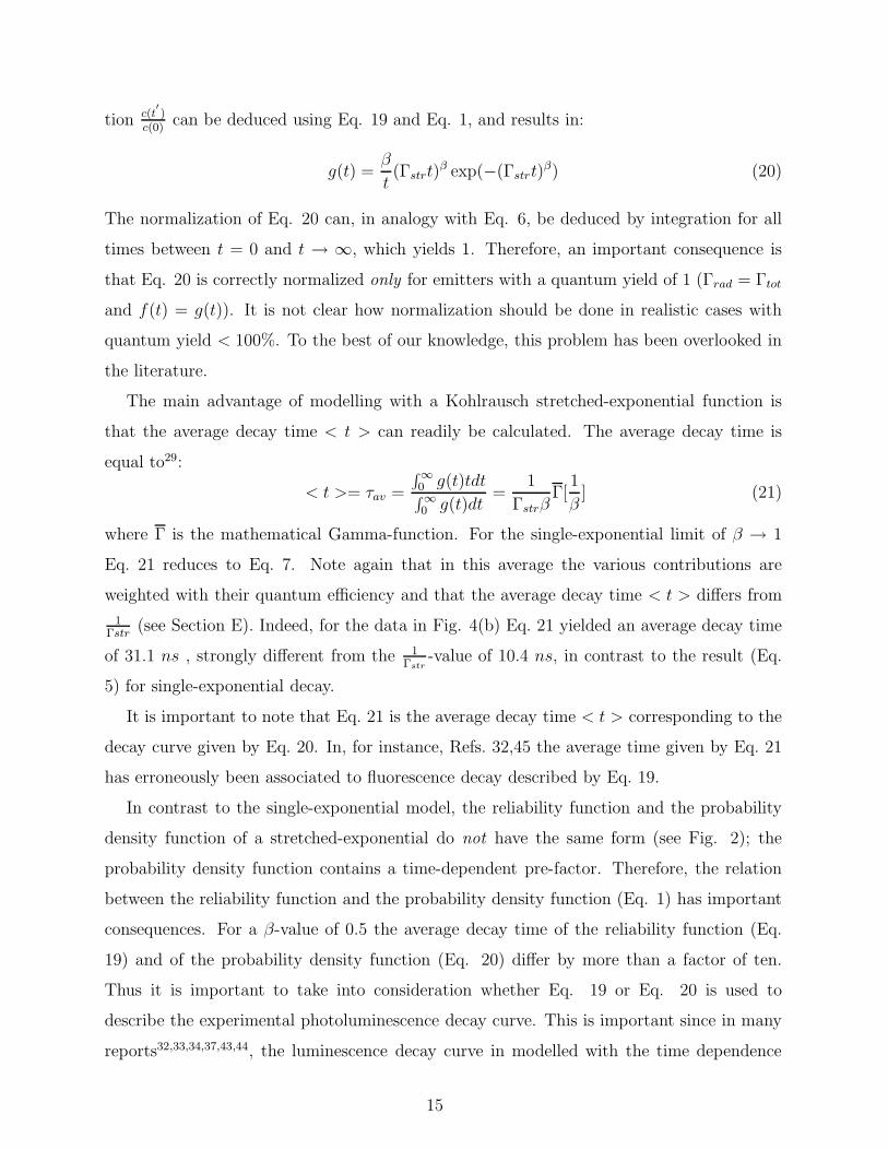
The main advantage of modelling with a Kohlrausch stretched-exponential function is

that the average decay time < t > can readily be calculated. The average decay time is

equal to29:

< t >= τav =

∫

∞

0 g(t)tdt∫

∞

0 g(t)dt=

1

ΓstrβΓ[

1

β] (21)

where Γ is the mathematical Gamma-function. For the single-exponential limit of β → 1

Eq. 21 reduces to Eq. 7. Note again that in this average the various contributions are

weighted with their quantum efficiency and that the average decay time < t > differs from

1Γstr

(see Section E). Indeed, for the data in Fig. 4(b) Eq. 21 yielded an average decay time

of 31.1 ns , strongly different from the 1Γstr

-value of 10.4 ns, in contrast to the result (Eq.

5) for single-exponential decay.

It is important to note that Eq. 21 is the average decay time < t > corresponding to the

decay curve given by Eq. 20. In, for instance, Refs. 32,45 the average time given by Eq. 21

has erroneously been associated to fluorescence decay described by Eq. 19.

In contrast to the single-exponential model, the reliability function and the probability

density function of a stretched-exponential do not have the same form (see Fig. 2); the

probability density function contains a time-dependent pre-factor. Therefore, the relation

between the reliability function and the probability density function (Eq. 1) has important

consequences. For a β-value of 0.5 the average decay time of the reliability function (Eq.

19) and of the probability density function (Eq. 20) differ by more than a factor of ten.

Thus it is important to take into consideration whether Eq. 19 or Eq. 20 is used to

describe the experimental photoluminescence decay curve. This is important since in many

reports32,33,34,37,43,44, the luminescence decay curve in modelled with the time dependence

15

of Eq. 19. We remark that while Eq. 19 can be used to account for the deviation from

single-exponential decay, it does not represent the true Kohlrausch function, but is simply an

alternative model. We argue that using the Kohlrausch stretched-exponential as a reliability

function to model the fraction c(t′

)c(0)

48 implies that the proper probability density function, i.e.,

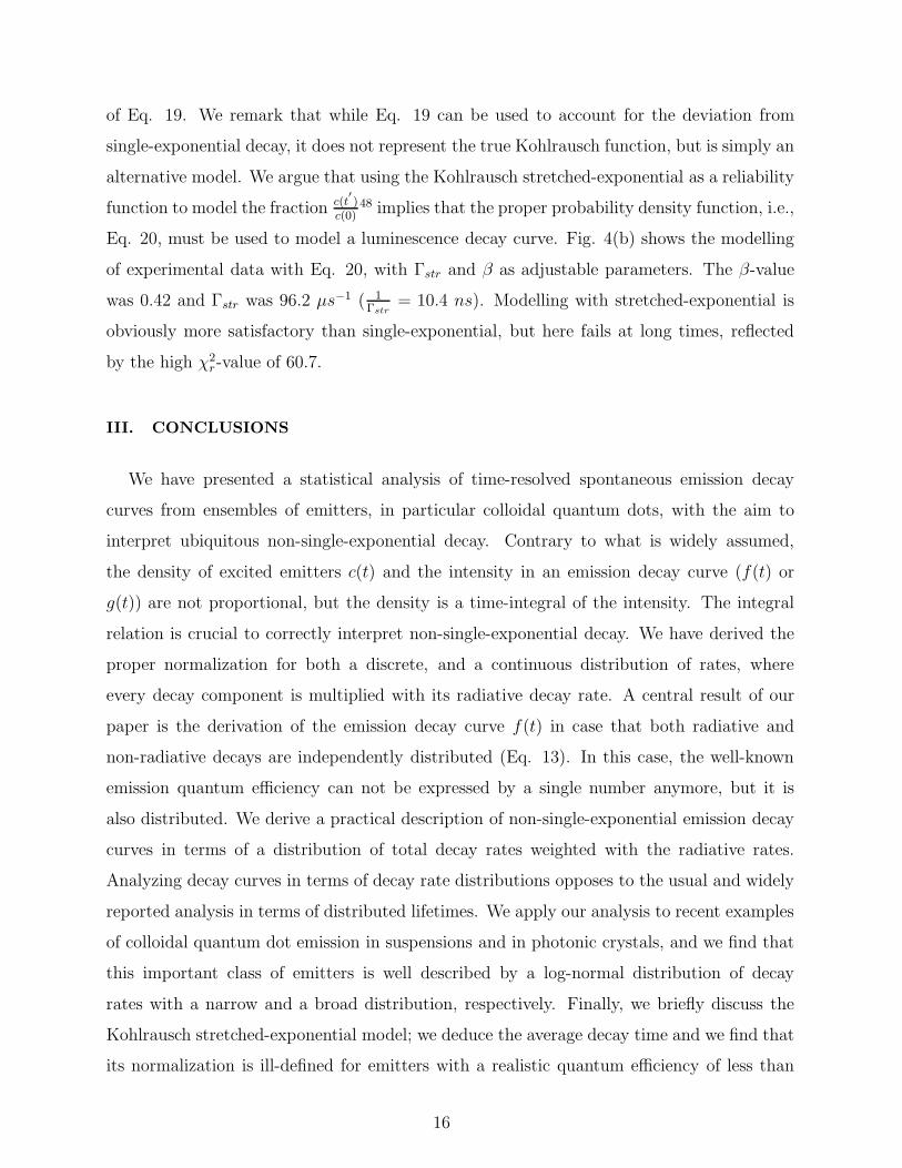
Eq. 20, must be used to model a luminescence decay curve. Fig. 4(b) shows the modelling

of experimental data with Eq. 20, with Γstr and β as adjustable parameters. The β-value

was 0.42 and Γstr was 96.2 µs−1 ( 1Γstr

= 10.4 ns). Modelling with stretched-exponential is

obviously more satisfactory than single-exponential, but here fails at long times, reflected

by the high χ2r-value of 60.7.

III. CONCLUSIONS

We have presented a statistical analysis of time-resolved spontaneous emission decay

curves from ensembles of emitters, in particular colloidal quantum dots, with the aim to

interpret ubiquitous non-single-exponential decay. Contrary to what is widely assumed,

the density of excited emitters c(t) and the intensity in an emission decay curve (f(t) or

g(t)) are not proportional, but the density is a time-integral of the intensity. The integral

relation is crucial to correctly interpret non-single-exponential decay. We have derived the

proper normalization for both a discrete, and a continuous distribution of rates, where

every decay component is multiplied with its radiative decay rate. A central result of our

paper is the derivation of the emission decay curve f(t) in case that both radiative and

non-radiative decays are independently distributed (Eq. 13). In this case, the well-known

emission quantum efficiency can not be expressed by a single number anymore, but it is

also distributed. We derive a practical description of non-single-exponential emission decay

curves in terms of a distribution of total decay rates weighted with the radiative rates.

Analyzing decay curves in terms of decay rate distributions opposes to the usual and widely

reported analysis in terms of distributed lifetimes. We apply our analysis to recent examples

of colloidal quantum dot emission in suspensions and in photonic crystals, and we find that

this important class of emitters is well described by a log-normal distribution of decay

rates with a narrow and a broad distribution, respectively. Finally, we briefly discuss the

Kohlrausch stretched-exponential model; we deduce the average decay time and we find that

its normalization is ill-defined for emitters with a realistic quantum efficiency of less than

16

100 %.

IV. ACKNOWLEDGMENTS

This work is part of the research program of both the ”Stichting voor Fundamenteel

Onderzoek der Materie (FOM)”, and ”Chemische Wetenschappen”, which are financially

supported by the ”Nederlandse Organisatie voor Wetenschappelijk Onderzoek (NWO)”.

∗ Electronic address: w.l.vos@utwente.nl; Webpage: www.photonicbandgaps.com

1 J. R. Lakowicz, Principles of Fluorescence Spectroscopy (Kluwer Academic/Plenum Publishers,

New York, Boston, Dordrecht, London, Moscow, 1999), 2nd ed.

2 I. L. Medintz, H. T. Uyeda, E. R. Goldman, and H. Mattoussi, Nature Materials 4, 435 (2005).

3 R. Loudon, The quantum theory of light, Oxford science publications (Oxford University Press,

Oxford,, 2001), 3rd ed.

4 S. A. Crooker, J. A. Hollingsworth, S. Tretiak, and V. I. Klimov, Physical Review Letters 89,

186802 (2002).

5 J. Y. Zhang, X. Y. Wang, and M. Xiao, Optics Letters 27, 1253 (2002).

6 K. H. Drexhage, Journal of Luminescence 1,2, 693 (1970).

7 R. M. Amos and W. L. Barnes, Physical Review B 55, 7249 (1997).

8 N. Danz, J. Heber, and A. Brauer, Physical Review A 66, 063809 (2002).

9 S. Astilean and W. L. Barnes, Applied Physics B-Lasers and Optics 75, 591 (2002).

10 M. Bayer, T. L. Reinecke, F. Weidner, A. Larionov, A. McDonald, and A. Forchel, Physical

Review Letters 86, 3168 (2001).

11 J. S. Biteen, D. Pacifici, N. S. Lewis, and H. A. Atwater, Nano Letters 5, 1768 (2005).

12 J. H. Song, T. Atay, S. F. Shi, H. Urabe, and A. V. Nurmikko, Nano Letters 5, 1557 (2005).

13 M. Fujita, S. Takahashi, Y. Tanaka, T. Asano, and S. Noda, Science 308, 1296 (2005).

14 A. Kress, F. Hofbauer, N. Reinelt, M. Kaniber, H. J. Krenner, R. Meyer, G. Bohm, and J. J.

Finley, Physical Review B 71, 241304 (2005).

15 P. Lodahl, A. F. van Driel, I. S. Nikolaev, A. Irman, K. Overgaag, D. Vanmaekelbergh, and

W. L. Vos, Nature 430, 654 (2004).

17

16 P. Foggi, L. Pettini, I. Santa, R. Righini, and S. Califano, Journal of Physical Chemistry 99,

7439 (1995).

17 V. I. Klimov and D. W. McBranch, Physical Review Letters 80, 4028 (1998).

18 F. V. R. Neuwahl, P. Foggi, and R. G. Brown, Chemical Physics Letters 319, 157 (2000).

19 A. Rosencwaig, Photoacoustics and Photoacoustic Spectroscopy (John Wiley & Sons, New York,

1980).

20 M. Grinberg, A. Sikorska, and A. Sliwinski, Physical Review B 67, 045114 (2003).

21 D. R. James and W. R. Ware, Chemical Physics Letters 126, 7 (1986).

22 A. Siemiarczuk, B. D. Wagner, and W. R. Ware, Journal of Physical Chemistry 94, 1661 (1990).

23 J. C. Brochon, A. K. Livesey, J. Pouget, and B. Valeur, Chemical Physics Letters 174, 517

(1990).

24 J. Wlodarczyk and B. Kierdaszuk, Biophysical Journal 85, 589 (2003).

25 S. F. Wuister, A. van Houselt, C. D. M. Donega, D. Vanmaekelbergh, and A. Meijerink, Ange-

wandte Chemie-International Edition 43, 3029 (2004).

26 I. S. Nikolaev, P. Lodahl, A. F. van Driel, and W. L. Vos, http://arxiv.org/abs/physics/0511133

(2005).

27 R. Kohlrausch, Annalen der Physik 91, 179 (1854).

28 L. A. Deschenes and D. A. Vanden Bout, Science 292, 255 (2001).

29 C. P. Lindsey and G. D. Patterson, Journal of Chemical Physics 73, 3348 (1980).

30 R. Kohlrausch, Annalen der Physik 91, 56 (1854).

31 R. Torre, P. Bartolini, and R. Righini, Nature 428, 296 (2004).

32 G. Schlegel, J. Bohnenberger, I. Potapova, and A. Mews, Physical Review Letters 88, 137401

(2002).

33 R. Chen, Journal of Luminescence 102, 510 (2003).

34 B. R. Fisher, H. J. Eisler, N. E. Stott, and M. G. Bawendi, Journal of Physical Chemistry B

108, 143 (2004).

35 D. L. Huber, Physical Review B 31, 6070 (1985).

36 F. Alvarez, A. Alegria, and J. Colmenero, Physical Review B 44, 7306 (1991).

37 M. Lee, J. Kim, J. Tang, and R. M. Hochstrasser, Chemical Physics Letters 359, 412 (2002).

38 P. Vergeer, T. J. H. Vlugt, M. H. F. Kox, M. I. den Hertog, J. van der Eerden, and A. Meijerink,

Physical Review B 71, 014119 (2005).

18

39 E. R. Dougherty, Probability and Statistics for the engineering, computing and physical sciences

(Prentice-Hall International, Inc., Englewood, New Jersey, 1990).

40 A. F. van Driel, G. Allan, C. Delerue, P. Lodahl, W. L. Vos, and D. Vanmaekelbergh, Physical

Review Letters 95, 236804 (2005).

41 R. Sprik, B. A. van Tiggelen, and A. Lagendijk, Europhysics Letters 35, 265 (1996).

42 D. R. James, Y.-S. Liu, P. De Mayo, and W. R. Ware, Chemical Physics Letters 120, 460

(1985).

43 K. C. Benny Lee, J. Siegel, S. E. D. Webb, S. Leveque-Fort, M. J. Cole, R. Jones, K. Dowling,

M. J. Lever, and P. M. W. French, Biophysical Journal 81, 1265 (2001).

44 M. N. Berberan-Santos, E. N. Bodunov, and B. Valeur, Chemical Physics 315, 171 (2005).

45 J. Kalkman, H. Gersen, L. Kuipers, and A. Polman, Physical Review B 73, 075317 (2006).

46 In the case of strong coupling in cavity quantum electrodynamics, the decay of even a single

emitter is not single-exponential. Experimental situations where this may be encountered are

emitters in a high-finesse cavity, or van Hove singularities in the LDOS of a photonic crystal.

47 In case of the stretched-exponential model the distribution of the rates is unknown and is

generally deduced by solving the following equation21,32,42,43,44: βt(Γstrt)

β exp(−(Γstrt)β) =

∫

∞

0 σ(Γ) exp(−Γt)dΓ where σ(Γ) is the distribution function of total decay rate weighted by

Γrad. To deduce σ(Γ) an inverse Laplace transform is applied. For β 6= 0.5 and β 6= 1 there

is no analytical solution of this equation and therefore it is difficult to deduce the distribution

function. This difficulty can be circumvented by modelling directly with a known distribution

function, as is shown in this paper.

48 We remark that in Refs. 27,29 capacitor discharge and dielectric relaxation are studied, which

are, in contrast to a fluorescence decay curve, indeed described by a reliability function.

19