QUANTUM EXPONENTIAL FUNCTION

QUANTUM EXPONENTIAL FUNCTION

S. L. WORONOWICZ∗

Department of Mathematical Methods in PhysicsFaculty of Physics, University of Warsaw

Hoza 74, 00-682 Warszawa, Polandand

Institute of Mathematics, Trondheim University, Norway

Received 15 February 1999

A special function playing an essential role in the construction of quantum “ax + b”-groupis introduced and investigated. The function is denoted by F~(r, %), where ~ is a constantsuch that the deformation parameter q2 = e−i~. The first variable r runs over non-zero realnumbers; the range of the second one depends on the sign of r: % = 0 for r > 0 and % = ±1for r < 0. After the holomorphic continuation the function satisfies the functional equation

F~(ei~r, %) = (1 + ei~/2r)F~(r,−%) .

The name “exponential function” is justified by the formula:

F~(R, ρ)F~(S, σ) = F~([R + S], σ) ,

where R, S are selfadjoint operators satisfying certain commutation relations and [R+S] isa selfadjoint extension of the sum R+ S determined by operators ρ and σ appearing in theformula. This formula will be used in a forthcoming paper to construct a unitary operatorW satisfying the pentagonal equation of Baaj and Skandalis.

0. Introduction

Quantum exponential functions appear in the following setting. One considers pairs

of closed operators (R,S) acting on a Hilbert space H satisfying certain carefully

chosen commutation relations C. These relations should imply that the operators

R and S are normal and SpR and SpS be contained in certain subset Λ ⊂ C.

Moreover the sum R+ S should be a well-defined closed normal operator with the

spectrum contained in the same set Λ. A continuous function F defined on Λ with

values in the unit circle in C is called a quantum exponential function if

F (R+ S) = F (R)F (S) (0.1)

for any pair (R,S) of operators satisfying the considered commutation relations.

The first example we obtain considering the following commutation relations:

R∗ = R, S∗ = S and RS = SR . (0.2)

Then Λ = R, F is a function of real variable and (0.1) is equivalent to the classical

exponential equation:

F (r + s) = F (r)F (s) (0.3)

∗Supported by Komitet Badan Naukowych, grant No 2 P0A3 030 14.

873

Reviews in Mathematical Physics, Vol. 12, No. 6 (2000) 873–920c©World Scientific Publishing Company

874 S. L. WORONOWICZ

for any r, s ∈ R. One of the solutions is F (r) = eir. Any other function satisfying

(0.3) is of the form Ft(r) = eitr, where t is a real number.

In the second example we consider the following relations:

RR∗ = R∗R, SS∗ = S∗S ,

SpR,SpS ⊂ Cq

and

RS = q2SR .

(0.4)

In these relations q is a real number, q < 1 and

Cq

= t ∈ C : t = 0 or |t| ∈ qZ .

The precise meaning of (0.4) is explained in [11] and [12] (such an explanation should

also be given for relations (0.2), where RS = SR means the strong commutation of

selfadjoint operators R,S). In this case a function F satisfying Eq. (0.1) is given

by the formula:

F (t) =∞∏k=0

1 + q2kt

1 + q2kt.

Any other function satisfying (0.1) is of the form Ft(r) = F (tr), where t ∈ Cq.

In this paper we consider the following commutation relations:

R∗ = R, S∗ = S ,

RS = q2SR .

(0.5)

In this case the deformation parameter q2 is a number of modulus 1. The precise

meaning of the relations is given in Sec. 2. We shall assume that

q2 = e−i~ , (0.6)

where ~ is a real number such that −π < ~ < π. This is the only assumption on

~ imposed in this paper. To construct deformed “ax+ b” group [15] we shall have

to assume some further restrictions on q. It turns out that the group exists on the

Hilbert space level (and on the C∗-level) provided ~ = ± π2k+3 , where k = 0, 1, 2, . . . .

In this case q is a root of 1.

We write R( S if the pair of selfadjoint operators (R,S) satisfies the relations

(0.5) in the sense explained in Sec. 2. The relation “(” is called Zakrzewski relation.

The theory of quantum exponential function based on the relations (0.5) does

not fit precisely into the scheme described above. If R and S are selfadjoint oper-

ators satisfying the Zakrzewski relation R ( S, then R + S is a symmetric, but

(in general) not a selfadjoint operator. In fact R + S is selfadjoint if and only if

(signR)(signS) ≥ 0. We shall show that selfadjoint extensions of R+S are labeled

by selfadjoint operators τ such that Sp τ ⊂ −1, 0, 1, τ anticommutes with R and S

and ker τ coincides with H((signR)(signS) ≥ 0). Operators τ are called reflection

operators.

Let ρ be a selfadjoint operator such that Sp ρ ⊂ −1, 0, 1, ρ anticommutes

with S, commutes with R and kerρ = H(R ≥ 0). Similarly let σ a selfadjoint

QUANTUM EXPONENTIAL FUNCTION 875

operator such that Spσ ⊂ −1, 0, 1, σ anticommutes with R, commutes with S

and kerσ = H(S ≥ 0). Then for any number α of modulus 1, the operator

τ = αρσ + ασρ (0.7)

satisfies all the conditions listed above. In what follows α = ieiπ2

2~ .

In our case instead of (0.1) we have to consider a more complicated equation

F (R, ρ)F (S, σ) = F ([R + S]τ , σ) , (0.8)

where [R + S]τ is the selfadjoint extension of R + S corresponding to a reflection

operator (0.7) and σ is an operator uniquely determined by R, S, ρ and σ. The

operator σ is selfadjoint, Sp σ ⊂ −1, 0, 1, σ anticommutes with [R + S]τ and

kerσ = H([R + S]τ ≥ 0). Now the function F = F (r, %) is a function of two

variables: r ∈ R and % ∈ −1, 0, 1.The exponential function equality (0.8) is closely related to the pentagonal equa-

tion

F (T, τ)F (S, σ)F (R, ρ) = F (R, ρ)F (S, σ) . (0.9)

In the forthcoming paper [15] we shall construct the quantum “ax+ b” group. This

construction uses the idea of Baaj and Skandalis [2], who pointed out that quantum

groups are determined by one unitary operator W ∈ B(H ⊗H) satisfying certain

simple conditions (see also [13]). In [15] we propose an explicit formula for W

related to the quantum “ax+ b” group. The main aim of the present paper is to

provide the computational tools for [15]. In particular (0.9) will be used to verify

that W satisfies the Baaj–Skandalis pentagonal equation.

We shall briefly describe the content of the paper. In Sec. 1 we introduce spe-

cial functions used in this paper. Among them we have the quantum exponential

function F~ and the related function Vθ. Various equalities and estimates are es-

tablished. Some boring computations are shifted to Appendices. This section is

entirely classical: no non-commutative quantity appears in it. We use the methods

of the theory of analytic functions of one variable.

The Zakrzewski commutation relations are introduced in Sec. 2. We indicate

the connection with the Heisenberg commutation relations. The most general pair

(R,S) of selfadjoint operators satisfying the Zakrzewski relations is described.

Section 3 is devoted to operators of the form Sf(R). The main result of this

section is contained in Theorem 3.1. We find when Sf(R) is selfadjoint and compute

in this case sign(Sf(R)). In particular the operator ei~/2RS is selfadjoint and

sign (ei~/2RS) = (signR)(signS).

The operator of the form Q = ei~/2RS + S is investigated in Secs. 4 and 5.

Clearly Q is symmetric. We show that Q is selfadjoint if and only if R ≥ 0. If this

is not the case then we look for selfadjoint extensions. It turns out that selfadjoint

extensions of Q are unitarily equivalent to S. The correponding unitary operators

coincide with F~(R, ρ), where F~ is the quantum exponential function and ρ are

reflection operators mentioned above:

[ei~/2RS + S]ρ = F~(R, ρ)∗SF~(R, ρ) . (0.10)


The main result of the paper is contained in Sec. 6. We prove the exponent

equation (0.8) and the pentagonal equation (0.9). To this end we use the method

similar to the one used in [11]. In principle it is based on the associativity of

addition:

[S + ei~/2ST−1] + T−1 = S + [ei~/2ST−1 + T−1] .

The most difficult part of the proof is to show that the formula remains valid, when

we pass to suitable selfadjoint extensions:

[[S + ei~/2ST−1]τ + T−1]σ

= [S + [ei~/2ST−1 + T−1]σ]ρ, (0.11)

where ρ = F~(S, σ)∗ρF~(S, σ). Using the unitary implementation (0.10) one can

easily show that (0.11) coincides with the most crucial formula (6.11) of the proof

of pentagonal equation. The proof of (0.11) is rather complicated. One has to keep

track of the domains of all selfadjoint operators appearing in this formula. As a

result, Sec. 6 is the most sophisticated in this paper.

In Sec. 7 we show that any function F satisfying the exponential equality (0.8) is

of the form: F (r, %) = F~(µr, s%). This result will be used to find all unitary repre-

sentations of quantum “ax+ b”-group. The last section deals with C∗-algebras and

affiliation relation. Quantum exponential function is used to formulate a condition

for a pair of selfdajoint operators to be affiliated with a C∗-algebra.

The paper uses heavily the theory of unbounded operators on Hilbert spaces

(cf. [1, 4, 6, 7]). We shall mainly use closed operators. The domain of an operator

a acting on a Hilbert space H will be denoted by D(a). We shall always assume

that D(a) is dense in H.

We shall use the functional calculus for systems of strongly commuting selfad-

joint operators. To explain the rather peculiar but very convenient notation used

in the paper, let us consider the pair of strongly commuting selfadjoint operators a

and b acting on a Hilbert space H. Then, by the spectral theorem

a =

∫ ⊕R2

λdE(λ, µ) , b =

∫ ⊕R2

µdE(λ, µ) ,

where dE(λ) is the common spectral measure associated with a, b. For any measur-

able (complex valued) function f of two variables,

f(a, b) =

∫ ⊕R2

f(λ, λ′)dE(λ, λ′).

Let χ be the logical evaluation of a sentence:

χ(false) = 0 ,

χ(true) = 1 .

If R is a two argument relation defined on real numbers, then f(λ, λ′) = χ(R(λ, λ′))

is a characteristic function of the set ∆ = (λ, λ′) ∈ R2 : R(λ, λ′) and (assuming

that ∆ is measurable) f(a, b) = E(∆). We shall write χ(R(a, b)) instead of f(a, b):

χ(R(a, b)) =

∫ ⊕R2

χ(R(λ, λ′))dE(λ, λ′) = E(∆) .


The range of this projection will be denoted by H(R(a, b)). The letter “H” in this

expression refers to the Hilbert space, where operators a, b act.

This way we gave meaning to the expressions: χ(a > b), χ(a2+b2 = 1), χ(a = 1),

χ(b < 0), χ(a 6= 0) and many others of this form. They are orthogonal projections

onto corresponding spectral subspaces. For example H(a = 1) is the eigenspace of

a corresponding to the eigenvalue 1 and χ(a = 1) is the orthogonal projection onto

this eigenspace. More generally if ∆ is a measurable subset of R, then H(a ∈ ∆) is

the spectral subspace of a corresponding to ∆ and χ(a ∈ ∆) is the corresponding

spectral projection.

1. Special Functions

The quantum exponential function is introduced in an axiomatic way. In this section

we formulate the conditions determining uniquely this function. The function is

then defined by an explicit formula and we verify that all the conditions hold.

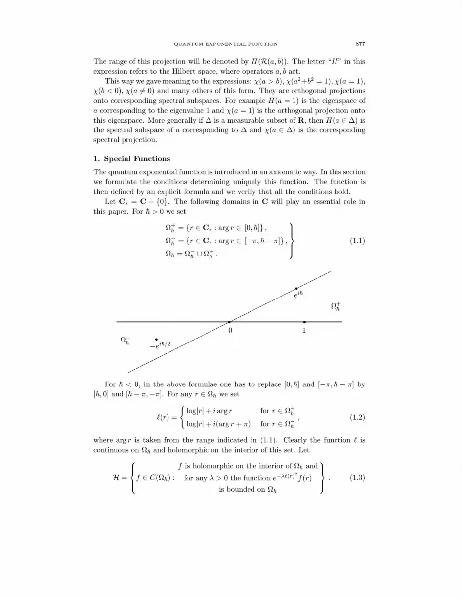
Let C∗ = C − 0. The following domains in C will play an essential role in

this paper. For ~ > 0 we set

Ω+~ = r ∈ C∗ : arg r ∈ [0, ~] ,

Ω−~ = r ∈ C∗ : arg r ∈ [−π, ~− π] ,Ω~ = Ω−~ ∪Ω+

~ .

(1.1)

r r

r

r

Ω+~

Ω−~

0 1

−ei~/2

ei~

For ~ < 0, in the above formulae one has to replace [0, ~] and [−π, ~ − π] by

[~, 0] and [~− π,−π]. For any r ∈ Ω~ we set

`(r) =

log|r|+ i arg r for r ∈ Ω+

~

log|r|+ i(arg r + π) for r ∈ Ω−~, (1.2)

where arg r is taken from the range indicated in (1.1). Clearly the function ` is

continuous on Ω~ and holomorphic on the interior of this set. Let

H =

f ∈ C(Ω~) :

f is holomorphic on the interior of Ω~ and

for any λ > 0 the function e−λ`(r)2

f(r)

is bounded on Ω~

. (1.3)


Replacing in this definition Ω~ by Ω+~ and Ω−~ we introduce the classes of functions

H+ and H−.

The vector space H (as well as H+ and H−) admits an interesting antiunitary

involution. For any f ∈ H and r ∈ Ω~ we set

f∗(r) = f(ei~r). (1.4)

One can easily verify that f∗ ∈ H and f∗∗ = f .

The quantum exponential function F~ investigated in this paper is a function of

two variables denoted by r and %. The first one runs over Ω~ whereas the second

assumes three values: −1, 0, 1 with the following restrictions: % = 0 for r ∈ Ω+~ and

% = ±1 for r ∈ Ω−~ . In other words, F~ is defined on the set

∆F = Ω−~ × −1, 1 ∪ Ω+~ × 0 .

In the following theorem we collect the characteristic properties of F~.

Theorem 1.1. There exists a unique function

F~ : ∆F −→ C

fulfilling the following five conditions:

(1) For all (r, %) ∈ ∆F such that r ∈ R we have:

|F~(r, %)| = 1 . (1.5)

(2) The functions F~(·, 0), F~(·, 0)−1 ∈ H+.

(3) The functions F~(·, 1), F~(·,−1), F~(·,−1)−1 ∈ H−.(4) For any (r, %) ∈ ∆F such that r ∈ R we have:

F~(ei~r, %) = (1 + ei~/2r)F~(r,−%) . (1.6)

(5)

limr→0

F~(r, %) = 1 . (1.7)

In addition the function F~ has the following properties:

(6) F~(−ei~/2, 1) = 0. This is the only zero of F~ on ∆F .

(7) In a neighbourhood of zero,

F~(r, %) = 1 +r

2i sin ~2+Ro(r, %) , (1.8)

where

limr→0

Ro(r, %)

r= 0 .

This is a stronger version of Statement (5).

(8) There exists the limit

lim<r→+∞

F~(−r, 1)

F~(r, 0)= α , (1.9)


where

α = i exp

iπ2

2~

. (1.10)

For real r we have a stronger result:

limr-realr→+∞

|r(F~(−r, 1)− αF~(r, 0))| = 1

sin ~2. (1.11)

(9) For any r ∈ Ω+~ we have

F~(r, 0) = C exp

(log r)2

2i~

F~(r

−1, 0) . (1.12)

In a neighbourhood of infinity

F~(r, 0) = C exp

(log r)2

2i~

[1− r−1

2i sin ~2

]+R+

∞(r) , (1.13)

where

lim<r→+∞

R+∞(r) = 0 ,

limr-realr→+∞

rR+∞(r) = 0 .

(10) For any r ∈ Ω−~ and % = ±1 we have

F~(r, %) = C α% exp

(log(−r))2

2i~

F~(r

−1, %) . (1.14)

In a neighbourhood of infinity

F~(r, %) = Cα% exp

(log(−r))2

2i~

[1− r−1

2i sin ~2

]+R−∞(r, %) , (1.15)

where

lim<r→−∞

R−∞(r, %) = 0 ,

limr-realr→−∞

rR−∞(r, %) = 0 .

In the last two points, the constant C = exp(2π~ + ~

2π ) π12 i, log r = log |r|+i arg r

and log(−r) = log |r|+ i(π+ arg r) = log r+ iπ, where arg r is taken from the range

indicated in (1.1).

In this section we find an explicit formula expressing F~(r, %) in terms of integrals

of elementary functions. We shall prove that F~(r, %) has the properties listed in

the above theorem. The uniqueness will be discussed later (cf. the end of Sec. 5).


The reader should notice that if a function F~(r, %) satisfies any of the conditions

(1)–(9) of the above theorem then the function F ′~(r, %) = F~(r, %) satisfies the same

conditions with ~ replaced by −~. It means that

F−~(r, %) = F~(r, %) . (1.16)

Due to this formula it is sufficient to consider the case ~ > 0.

To simplify the notation we set θ = 2π~ . Clearly θ > 2. For any (r, %) ∈ ∆F we

have

F~(r, %) = [1 + i%(−r)π~ ]Vθ(log r) . (1.17)

In this formula log r = log|r| + i arg r and (−r)π~ = |r|π~ exp( iπ~ [π + arg r]), where

arg r is taken from the range indicated in (1.1). Vθ is a meromorphic function on

C such that

Vθ(x) = exp

1

2πi

∫ ∞0

log(1 + a−θ)da

a+ e−x

(1.18)

for all x ∈ C such that |=x| < π. For real r we have:

F~(r, %) =

Vθ(log r) for r > 0 and % = 0

[1 + i%|r|π~ ]Vθ(log|r| − πi) for r < 0 and % = ±1 .(1.19)

Lemma 1.1. Let θ be a positive number. Then the integral

Wθ(x) =

∫ ∞0

log(1 + a−θ)da

a+ e−x(1.20)

is convergent for any x ∈ C such that |=x| < π. The function Wθ introduced in

this way is holomorphic in the strip x ∈ C : |=x| < π. It admits a continuous

extension to the closure of this strip. Moreover we have:

Wθ(x) +Wθ(−x) =θx2

2+ (θ + θ−1)

π2

6, (1.21)

W1/θ(x) = Wθ(x/θ) , (1.22)

Wθ(x+ πi)−Wθ(x− πi) = 2πi log(1 + eθx) . (1.23)

In (1.23) the variable x is real, whereas in (1.21) and (1.22) x ∈ C and |=x| ≤ π.If θ > 2, then

Wθ(x) =πex

sin(πθ

) − πe2x

2 sin(

2πθ

) +R(x) , (1.24)

where

e−2xR(x) −→ 0 , (1.25)

when <x→ −∞ whereas =x stays in a compact subset of the interval ]− π, π[.

The proof of this lemma is not very fascinating. It uses the standard methods of

the theory of holomorphic functions of one variable. The boring details are shifted

to Appendix A.


Comparing (1.18) with (1.20) we see that

Vθ(x) = exp

1

2πiWθ(x)

. (1.26)

Taking into account (1.22) and (1.23) we obtain:

V1/θ(x) = Vθ(x/θ) , (1.27)

Vθ(x+ πi) = (1 + eθx)Vθ(x− πi) . (1.28)

Inserting in (1.28) x/θ instead of x and using (1.27) we obtain

V1/θ(x+ πθi) = (1 + ex)V1/θ(x− πθi) .

Replacing now 1/θ by θ we get

Vθ

(x+

πi

θ

)= (1 + ex)Vθ

(x− πi

θ

). (1.29)

Remark 1.1. Equation (1.28) is essentially the same as functional equation defin-

ing function s in [3].

According to (1.26), the function Vθ is holomorphic and has no zeroes in the

strip x ∈ C : |=x| < π. Due to (1.28), it admits an analytical continuation to

a meromorphic function defined on the whole plane C. The extended function has

zeroes at the points

x = (2k + 1)πi+ (2l + 1)πi/θ , (1.30)

where k, l = 0, 1, 2, . . . . The poles are located at points −x, where x is given by

(1.30). Multiplicity of the zero (the pole respectively) at the point x (−x respec-

tively) equals to the number of pairs (k, l) of nonnegative integers satisfying the

relation (1.30). If θ is irrational, then all zeroes and poles are simple.

Replacing in (1.29) x by x+ πiθ

we obtain

Vθ

(x+

2πi

θ

)= (1 + eπi/θex)Vθ(x) . (1.31)

Taking into account (1.21) we get

Vθ(x)Vθ(−x) = Cθ exp

θx2

4πi

, (1.32)

where Cθ = exp(θ + θ−1) π12 i. Clearly Wθ(x) is real for x-real. Therefore

|Vθ(x)| = 1 (1.33)

for all x ∈ R. Taking the square of the both sides and performing analytical

continuation we get

Vθ(x)Vθ(x) = 1 (1.34)


and |Vθ(x)| |Vθ(x)| = 1. In particular |Vθ(x+πi)| |Vθ(x−πi)| = 1 for all x ∈ R. On

the other hand, due to (1.28) |Vθ(x+ πi)| = |1 + eθx| |Vθ(x− πi)|. Therefore

|Vθ(x− πi)| = |1 + eθx|− 12 (1.35)

for any x ∈ R. Combining (1.34) with (1.32) we obtain

Vθ(x) = Cθ exp

θx2

4πi

Vθ(−x) (1.36)

for all x ∈ C.

In further computations we set θ = 2π~ , where 0 < ~ < π. Then θ > 2 and using

(1.24) and (1.25) we get

V 2π~

(x) = 1 +ex

2i sin ~2− e2x−i~/2

4 sin~ sin ~2+R1(x) , (1.37)

where

e−2xR1(x) −→ 0 , (1.38)

when <x → −∞ whereas |=x| ≤ ~/2. It is enough to assume that (=x)e<x stays

bounded. Indeed, replacing in (1.31) θ by 2π~ and inserting (1.37) instead of Vθ(x)

we get after simple computations:

R1(x+ i~) = (1 + ei~/2ex)R1(x) . (1.39)

Let ω be a product of n factors of the form 1+ex with the same <x < 0. Elementary

computations show that

exp

− ne<x

1− e<x≤ |ω| ≤ expne<x .

Now, taking into account (1.39) can easily show that (1.38) holds when <x→ −∞whereas (=x)e<x stays bounded. In particular

limt→+∞

Vθ(xo + tλ) = 1 (1.40)

for any xo, λ ∈ C such that =λ < 0.

To prove the manageability of the multiplicative unitary for “ax+ b” quantum

group [15] we have to compute the Fourier transform of Vθ. It turns out that it is

expressed by the same function. Setting θ = 2π~ we have

1√2π~

∫`

Vθ

(y − i~

2− iπ

)eiy2

2~ eixy~ dy = C′~ Vθ(x) . (1.41)

In this formula C′~ is the phase factor equal to expi(π4 + ~24 + π2

6~ ), the path ` goes

along the real axis from −∞ to ∞ rounding the pole of the integrand at the point

0 from above. The integral should be understood in the sense of the distribution

theory; before comparing the numerical values of the both sides one has to multiply


them by a test function of x and integrate with respect to x (on the left-hand side

the integral with respect to y should be taken after that with respect to x). The

proof of (1.41) is given in Appendix B.

Now we are able to show that the function (1.17) satisfies conditions (1)–(10)

of Theorem 1.1. Condition (1) follows from (1.33) and (1.35). For r > 0 formula

(1.6) coincides with (1.31). To prove it for r < 0 it is sufficient to notice that (−r)π~changes sign, when arg r increases by ~. Condition (4) is verified. Conditions (7)

and (5) follows immediately from (1.37).

Inserting in (1.36) θ = 2π/~ we obtain (1.12). Combining (1.12) with (1.8) we

get (1.13), with

R+∞(r) = C exp

(log r)2

2i~

Ro(r, 0) .

Therefore

|R+∞(r)| = |r|

arg r~ |Ro(r, 0)|

and Condition (7) assures the correct asymptotic behavior of R+∞(r). Condition (9)

is verified.

To prove Condition (10) assume that r ∈ Ω−~ and % = ±1. Then

F~(r, %)

F~(r−1, %)

=V 2π~

(log r)[1 + i%(−r)π~ ]

V 2π~

(−log r)[1 + i%(−r)−π~ ]

= C 2π~

exp

(log r)2

2i~

1 + i%(−r)π~

1− i%(−r)−π~

= C 2π~

exp

(log r)2

2i~

i%(−r)π~

= i%C 2π~

exp

(log r)2 + 2πi log(−r)

2i~

.

In second step of the above computations we used (1.36). Remembering that

log(−r) = log r + iπ we obtain

F~(r, %)

F~(r−1, %)

= i%C 2π~

exp

(log(−r))2

2i~+iπ2

2~

= %αC 2π

~exp

(log(−r))2

2i~

,

where α is given by (1.10). Formula (1.14) is verified. Combining this formula with

(1.8) we obtain (1.15). Condition (10) is verified.

To verify Condition (8) we have to compute the limits (1.9) and (1.11). Using

asymptotic formulae (1.13) and (1.15) one can easily show that the limits exist and

have the correct values.

Definition (1.26) shows that V 2π~

(x) 6= 0 for all x ∈ C such that |=x| ≤ π.

Therefore F~(r, %) = 0 if and only if r ∈ Ω−~ , % = ±1 and 1 + (−r)π~ = 0. One can

easily check that this is the case if and only if r = −ei~/2 and % = 1. Condition (6)

is verified.


Finally using (1.7) and the asymptotic behavior (1.13) and (1.15) and remem-

bering that F~(·, 0) has no zero in Ω+~ and F~(·,−1) has no zero in Ω−~ one can easily

show that F~(·, 0), F~(·, 0)−1 ∈ H+ and F~(·, 1), F~(·,−1), F~(·,−1)−1 ∈ H−. The

reader should notice that F~(·, 1)−1 /∈ H−, because the function F~(·, 1) has a zero

point in Ω−~ . Conditions (2) and (3) are verified.

2. Zakrzewski Commutation Relations

Let R and S be selfadjoint operators acting on a Hilbert space H. If signR com-

mutes with S and R commutes with signS, then

H = H00 ⊕H0S ⊕HR0 ⊕HRS , (2.1)

where H00 = kerR ∩ kerS, H0S = kerR ∩ (kerS)⊥, HR0 = (kerR)⊥ ∩ kerS and

HRS = (kerR)⊥∩(kerS)⊥. Clearly operators R and S respect the above direct sum

decomposition and |R| and |S| are selfadjoint, strictly positive on HRS . Therefore

one can consider one parameter groups of unitaries (|R|iτ )τ∈R and (|S|iτ )τ∈R acting

on HRS .

Definition 2.1. We say that the operators R and S satisfy the Zakrzewski com-

mutation relations and write R( S if:

(1) signR commutes with S and R commutes with signS,

(2) On the subspace HRS = (kerR)⊥ ∩ (kerS)⊥, the groups of unitaries satisfy the

canonical commutation relations in the Weyl form:

|R|iτ |S|iτ ′ = ei~ττ′ |S|iτ ′ |R|iτ (2.2)

for any τ, τ ′ ∈ R. The pair is called non-degenerate if kerR = kerS = 0. This is

the case if and only if HRS = H.

One can easily check that R( S if and only if R commutes with signS and for

any τ ∈ R

|S|−iτR |S|iτ = e~τR . (2.3)

The latter equation should hold on the subspace (kerS)⊥.

Similarly R( S if and only if S commutes with signR and for any τ ∈ R

|R|iτS|R|−iτ = e~τS . (2.4)

The latter equation should hold on the subspace (kerR)⊥.

Let R and S be selfadjoint operators acting on a Hilbert space H. Assume

that R( S. Then the compositions RS and SR are densely defined closeable

operators, D(RS) is a core for S and D(SR) is a core for R. In what follows, the

closures of RS and SR will be denoted by RS and SR. It turns out that R and

S satisfy the commutation relation of the Manin plane: D(RS) = D(SR) and

RSx = q2SRx (2.5)


for any x ∈ D(SR). The reader should notice that the condition (2.5) is much

weaker than the relation R( S. For example (2.5) remains unchanged, when ~ is

replaced by ~+2π, whereas (2.2) is very sensitive to the choice of ~ solving Eq. (0.6).

We shall use the following simple statement:

Proposition 2.1. Let R and S be selfadjoint operators acting on a Hilbert space

H. Assume that R( S. Then:

(1) If kerS = 0, then S−1 ( R.

(2) If kerR = 0, then S ( R−1.

One can easily describe the structure of Hilbert space given by a pair (R,S)

of selfadjoint operators satisfying the relation R ( S. We already know that the

operators R and S respect the decomposition (2.1). On H00 both operators vanish.

On HR0 the operator S vanishes, whereas R is any selfadjoint operator. Similarly

on H0S , R vanishes whereas S is any selfadjoint operator (if one of the operators

vanish then the relation imposes no condition on the other one). On HRS the pair

is non-degenerate.

To describe nondegenerate pairs (R,S) of selfadjoint operators satisfying the

Zakrzewski relation we shall use position and momentum operators of a quantum

mechanical particle moving on R. Let (q, p) be an irreducible pair of selfadjoint

operators acting on a Hilbert space L such that the Heisenberg–Weyl commutation

relations:

eiτ qeiτ′p = ei~ττ

′eiτ′peiτ q

are satisfied for all τ, τ ′ ∈ R. In short [p, q] = i~I. Irreducibility means that the

only operators on L commuting with eiτ q and eiτ′p are scalar multiples of I. By

the famous Stone–von Neumann theorem [9], the pair (q, p) is unique up to unitary

equivalence. In Schrodinger representation L = L2(R) and

(qx)(t) = tx(t) , (px)(t) = i~dx(t)

dt. (2.6)

By definition a square integrable function x belongs to D(q) iff the product tx(t) is

square-integrable. Similarly x ∈ D(p) iff the derivative (understood in the sense of

the distribution theory) dx(t)dt

is a square-integrable function. In Sec. 4 we shall use

another representation: L = L2(R+) and

(qx)(s) = i~[−x(s)

2+

d

ds(sx(s))

], (px)(s) = −(log s)x(s) . (2.7)

Now a square integrable function x belongs to D(q) (x ∈ D(p) respectively) iff the

function dds

(sx(s)) ((log s)x(s) respectively) is square integrable on R+. The two

representations are related by the unitary Mellin transform:

x(s) =1√

2π|~|s

∫R

s−it~ x(t)dt .

With the notation introduced above we have:


Theorem 2.1. Let u and v be two commuting unitary involutions acting on a

Hilbert space K : u = u∗ = u−1, v = v∗ = v−1 and uv = vu. Then the pair

(R,S) = (u⊗ eq, v ⊗ ep) is a non-degenerate pair of selfadjoint operators acting on

L2(R,K) = K ⊗ L2(R) and R( S. Conversely any nondegenerate pair (R,S) of

selfadjoint operators satisfying the Zakrzewski relation R( S is unitarily equivalent

to a pair (u⊗ eq, v ⊗ ep) described above.

Proof. Only the last statement needs a proof. Let (R,S) be a non-degenerate pair

of selfadjoint operators acting on a Hilbert spaceH and R( S. Then the operators

log|R| and log|S| are selfadjoint and satisfy the Heisenberg commutation relation

in the Weyl form. By the Stone–von Neumann theorem [9] the pair (log|R|, log|S|)is unitarily equivalent to the direct sum of a certain number of copies of (q, p).

Denoting the multiplicity by N we may identify H with K ⊗ L (where K is an

N -dimensional Hilbert space) in such a way that

logR = I ⊗ q , logS = I ⊗ p . (2.8)

Irreducibility of (q, p) implies that any operator Q commuting with q and p is of

the form Q = Qo ⊗ I, where Qo is an operator acting on K. In particular

signR = u⊗ I , signS = v ⊗ I , (2.9)

where u and v are commuting unitary involutions acting on K. Combining (2.8)

with (2.9) we obtain

R = u⊗ eq , S = v ⊗ ep . (2.10)

The number N = dimK will be called the multiplicity of the pair (R,S). Clearly

N = N++ +N+− +N−+ +N−− ,

where N±± = dimK(u = ±1, v = ±1). Two nondegenerate pairs of selfadjoint

operators satisfying the Zakrzewski relation are unitarily equivalent iff they have

the same numbers N±±.

3. Analytical Implications of the Zakrzewski Relation

The selfadjoint operators satisfying the Zakrzewski relation have interesting ana-

lytical properties. On the formal level the relation RS = q2SR = e−i~SR imply

that f(ei~R)S = Sf(R). In this section we give the precise meaning to the latter

formula and find a class of functions f for which it holds. In what follows we use

functional calculus of selfadjoint operators. If R is a selfadjoint operator and f is a

measurable function defined on SpR, then by definition

f(R) =

∫f(λ)dER(λ) ,

where dER(λ) is the spectral measure associated with R. If kerR = 0, then

ER(0) = 0 and f(λ) need not be defined at λ = 0. Using the involution (1.4)


we have

f(R)∗ = f∗(ei~R) (3.1)

for any f ∈ H and any selfadjoint operator R. We start with the following:

Proposition 3.1. Let R and S be selfadjoint operators acting on a Hilbert space

H such that kerR = 0, R( S and g be a bounded function on Ω~. Assume that

g ∈ H. Then g(R)D(S) subsetD(S) and for any x ∈ D(S) we have

g(ei~R)Sx = Sg(R)x . (3.2)

Remark 3.1. If R is strictly positive, then it is sufficient to have function g defined

on Ω+~ only. Similarly if R < 0 then g may be restricted to Ω−~ .

Proof. For S = 0 the statement is trivial. Remembering that signS commutes

with R we may assume that S is strictly positive.

Let Σ be the strip τ ∈ C : 0 < =τ < 1 and H(Σ) be the space of all continuous

functions on Σ, holomorphic on Σ. Clearly H(Σ) endowed with the sup norm is a

Banach space.

For any λ ∈ R and τ ∈ Σ we set: ϕλ(τ) = g(e~τλ). Then ϕλ ∈ H(Σ) and

‖ϕλ‖ ≤ C, where C = sup|g(r)| : r ∈ Ω~. Therefore∫R

ϕλdµ(λ) ∈ H(Σ) (3.3)

for any (complex valued) finite measure dµ(λ) on R.

Let dER(λ) be the spectral measure of the selfadjoint operator R, x, y ∈ D(S)

and dµ(λ) = (y|dER(λ)Sx). Then∫R

ϕλ(τ)dµ(λ) = (y|g(e~τR)Sx)

and formula (3.3) shows that the function

Σ 3 τ −→ (y|g(e~τR)Sx) ∈ C

is continuous and holomorphic on the interior of Σ.

Remembering that x, y ∈ D(S) one can easily show that the mappings

Σ 3 τ −→ S1+iτx ∈ H ,

Σ 3 τ −→ Siτy ∈ H

are continuous. The first one is holomorphic whereas the second one is antiholo-

morphic on Σ. Therefore the function

Σ 3 τ −→ (Siτy|g(R)S1+iτx) ∈ C

is continuous and holomorphic on Σ.


Assume for the moment that τ is real. Using (2.3) we obtain

(Siτy|g(R)S1+iτx) = (y|S−iτg(R)S1+iτx) = (y|g(e~τR)Sx) .

By holomorphic continuation this equality holds for all τ ∈ Σ. In particular for

τ = i we obtain

(Sy|g(R)x) = (y|g(ei~R)Sx) .

This relation holds for all y ∈ D(S). Remembering that S is selfadjoint we see that

g(R)x ∈ D(S) and Sg(R)x = g(ei~R)Sx.

Let R ( S, where (R,S) is a pair of selfadjoint operators acting on the same

Hilbert space H such that kerR = 0. We shall use the function `(·) introduced by

(1.2). Then for any λ > 0 the operator e−λ`(R)2

is bounded and converges strongly

to I, when λ→ +0. Therefore the domain

D0 =⋃λ>0

e−λ`(R)2

D(S) , (3.4)

is dense in H. With this notation we have:

Proposition 3.2. Let f ∈ H. Then

(0) D0 ⊂ D(f(R))

(1) f(R)D0 ⊂ D0,

(2) D0 ⊂ D(S),

(3) SD0 ⊂ D(f(ei~R)).

Proof. Let λ > 0. One can easily verify that the function g(r) = e−λ`(r)2

sat-

isfies the assumptions of Proposition 3.1. Therefore e−λ`(R)2

D(S) ⊂ D(S) and

Statement (2) follows.

Now, let f ∈ H and λ > 0. Then the function g(r) = f(r)e−λ`(r)2

is bounded.

Therefore e−λ`(R)2

H ⊂ D(f(R)) and Statement (0) follows. One can easily verify

that the function g(r) considered in this paragraph satisfies the assumptions of

Proposition 3.1. Therefore

f(R)e−λ`(R)2

D(S) ⊂ D(S) ,

f(R)e−2λ`(R)2

D(S) ⊂ e−λ`(R)2

D(S) ⊂ D0

and Statement (1) follows.

Let x ∈ D0. Then

x = e−λ`(R)2

x′ , (3.5)

where x′ ∈ D(S) and λ > 0. Formula (3.2) shows that

e−λ`(ei~R)2

Sx′ = Sx .

If f ∈ H then the function f(r)e−λ`(r)2

is bounded, f(ei~R)e−λ`(ei~R)2 ∈ B(H) and

Sx = e−λ`(ei~R)2

Sx′ ∈ D(f(ei~R)). Statement (3) is proved.


Let (R,S) be a pair of selfadjoint operators acting on a Hilbert space H such

that R ( S and kerR = 0, and let f ∈ H. Proposition 3.2 shows that the

compositions S f(R) and f(ei~R) S are densely defined (their domains contain

D0). Taking into account (3.1) we see that the adjoints (S f(R))∗ ⊃ f∗(ei~R) Sand (f(ei~R)S)∗ ⊃ Sf∗(R) are densely defined. Therefore Sf(R) and f(ei~R)Sare closeable operators. In what follows their closures will be denoted by Sf(R)

and f(ei~R)S.

Theorem 3.1. Let (R,S) be a pair of selfadjoint operators acting on a Hilbert

space H such that R ( S and kerR = 0, and D0 be the domain introduced by

(3.4). Then for any f ∈ H we have:

(0) D0 is a core for f(ei~R)S,

(1) (f(ei~R)S)∗ = Sf∗(R),

(2) f(ei~R)S ⊂ Sf(R),

(3) If moreover f−1 ∈ H, then f(ei~R)S = Sf(R),

(4) If f∗ = f, then f(ei~R)S is symmetric,

(5) If f−1 ∈ H and f∗ = f, then f(ei~R)S is selfadjoint and R( f(ei~R)S.

If R > 0 (R < 0 respectively), then one may replace H by H+ (H− respectively).

Proof Ad (1) and (0). We already know that (f(ei~R)S)∗ ⊃ Sf∗(R). Therefore

it is sufficient to prove the converse inclusion. Let y ∈ D((f(ei~R)S)∗) and z =

(f(ei~R)S)∗x. Then

(y|f(ei~R)Sx) = (z|x) (3.6)

for any x ∈ D(f(ei~R)S). In particular (cf. Statements (3) and (4) of Proposi-

tion 3.2) this relation holds for all x ∈ D0. Therefore

(y|f(ei~R)Se−λ`(R)2

x′) = (z|e−λ`(R)2

x′)

for any λ > 0 and x′ ∈ D(S). Using (3.2) we get

(y|f(ei~R)e−λ`(ei~R)2

Sx′) = (z|e−λ`(R)2

x′)

and

(f∗(R)e−λ`∗(R)2

y|Sx′) = (e−λ`(R)2

z|x′) .

This relation holds for all x′ ∈ D(S). Remembering that S is selfadjoint we obtain

f∗(R)e−λ`∗(R)2

y ∈ D(S), e−λ`∗(R)2

y ∈ D(Sf∗(R)) and

Sf∗(R)e−λ`∗(R)2

y = e−λ`(R)2

z .

This relation holds for any λ > 0. Sf∗(R) is a closed operator. Setting λ→ +0, we

obtain: y ∈ D(Sf∗(R)) and Sf∗(R)y = z. This way we showed that (f(ei~R)S)∗ ⊂Sf∗(R) and Statement (1) follows.

The reader should notice that using the relation (3.6) we restricted the range of

variable x to the set D0. It shows that f(ei~R)S and its restriction to D0 have the

same adjoint. Therefore they have the same closure. In other words, D0 is a core

for f(ei~R)S.


Ad (2). Let x ∈ D0. Then x = e−λ`(R)2

x′, where x′ ∈ D(S) and λ > 0.

Formula (3.2) shows that Sf(R)x = f(ei~R)e−λ`(ei~R)2

Sx′. In particular for f = 1

we get Sx = e−λ`(ei~R)2

Sx′. Comparing the two formulae we obtain

f(ei~R)Sx = Sf(R)x .

This formula holds for all x ∈ D0. Remembering that D0 is a core for f(ei~R)S we

obtain f(ei~R)S ⊂ Sf(R).

Ad (3). It is sufficient to show that D0 is a core for Sf(R). Let x ∈ D(Sf(R)).

Then x ∈ D(f(R)) and y = f(R)x ∈ D(S). Therefore f(R)e−λ`(R)2

x = e−λ`(R)2

y ∈D0 for any λ > 0. In this point we assume that f−1 ∈ H. By Statement (1) of

Proposition 3.2, f(R)−1D0 ⊂ D0 and

e−λ`(R)2

x ∈ D0 . (3.7)

Using (3.2) we obtain

Sf(R)e−λ`(R)2

x = e−λ`(ei~R)2

Sf(R)x .

The reader should notice that e−λ`(R)2

x(e−λ`(ei~R)2

Sf(R)x respectively) converges

to x (to Sf(R)x respectively) when λ→ +0. Taking into account (3.7) we see that

D0 is a core for Sf(R).

Ad (4) and (5). Inserting f∗ = f in Statement (1) and using Statement (2) we

get f(ei~R)S ⊂ (f(ei~R)S)∗. It means that f(ei~R)S is symmetric. If in addition

f−1 ∈ H then (cf. Statement (3)) instead of inclusion we have equality and f(ei~R)S

is selfadjoint. To prove the Zakrzewski relation R ( f(ei~R)S it is sufficient to

notice that signR and |R|iτ commute with f(ei~R). Let f ∈ H. One can easily verify that f∗ = f if and only if f(ei~/2r) is real for

any r ∈ R. Assume that this is the case and that f−1 ∈ H. Then f has no zeroes

on Ω~ and sign f(ei~/2r) (for real r) depends only on sign r. If f(± ei~/2) > 0,

then f = g2, where g =√f and the branch of the square root is chosen in such

a way that g(± ei~/2) > 0. Clearly g ∈ H and g = g∗. Then g(ei~R)∗ = g(R),

g(ei~R)S ⊂ Sg(R) and for any x ∈ D0 we have

(x|f(ei~R)Sx) = (x|g(ei~R)2Sx) = (g(R)x|Sg(R)x) .

Remembering that D0 is a core for f(ei~R)S and that the operatorsR and S respect

the direct sum decomposition H = H(S < 0)⊕H(S = 0)⊕H(S > 0) we see that

signf(ei~R)S coincides with signS. One can easily modify the above considerations

to include all four possible combinations of signs of f(± ei~/2). This way we obtain:


space H such that R( S and kerR = 0 and f be a function on Ω~ such that f,

f−1 ∈ H and f = f∗. Then

sign f(ei~R)S = (sign f(ei~/2R))(signS) .

If R > 0 (R < 0 respectively), then one may replace Ω~ and H by Ω+~ and H+ (Ω−~

and H− respectively).


Example 3.1. Let f(r) = e−i~/2r. Then f, f−1 ∈ H and f∗ = f . Therefore

ei~/2RS is selfadjoint, sign ei~/2RS = (signR)(signS) and R( ei~/2RS. One can

easily verify that ei~/2RS( S. The reader should notice that we need not assume

that kerR = 0. Indeed the assertions we made are trivial if R = 0 (this is the

case not covered by Theorems 3.1 and 3.2).

Assume now that R and S are strictly positive. So is ei~/2RS. We claim that

(ei~/2RS)ik) = e−i~2 k

2

RikSik

= ei~2 k

2

SikRik . (3.8)

Indeed, using (2.2) one can easily show that the second equality holds and that

(e−i~2 k

2

RikSik)k∈R is a one parameter group of unitaries. Therefore there exists a

strictly positive operator T such that

T ik = e−i~2 k

2

RikSik

for all k ∈ R. Performing analytical continuation and setting k = −i we obtain

T = ei~/2RS and (3.8) follows.

4. Properties of (I+ei~~/2R)S

Throughout this section R and S are selfadjoint operators acting on a Hilbert space

H such that R ( S. We shall consider the operator Q = (ei~/2R + I)S. By

definition (cf. previous section) Q is the closure of the composition Q0 = (ei~/2R+

I) S. We shall prove that Q0 is closed.

Let (xn)n∈N be a sequence of elements of D(Q0) converging to a vector x∞ ∈ Hsuch that (Q0xn)n∈N converges to a vector y ∈ H. Then xn ∈ D(S), Sxn ∈ D(R)

and (ei~/2R + I)Sxn → y. The selfadjointness of R implies that −e−i~/2 /∈ SpR.

Therefore the operator ei~/2R+I has a bounded inverse and Sxn → (ei~/2R+I)−1y.

Remembering that S is closed we see that x∞ ∈ D(S) and Sx∞ = (ei~/2R+ I)−1y.

Therefore Sx∞ ∈ D(R), x∞ ∈ D(Q0) and Q0x∞ = (ei~/2R+ I)Sx∞ = y. It shows

that Q0 is closed, Q = Q0 and

D(Q) = x ∈ D(S) : Sx ∈ D(R) = D(ei~/2RS) ∩D(S) .

Therefore

Q = ei~/2RS + S . (4.1)

Proposition 4.1. The operator Q = ei~/2RS + S is symmetric. The adjoint

Q∗ = S(I + e−i~/2R). If R ≥ 0 then Q is selfadjoint.

Proof. If R = 0, then (I + ei~/2R)S = S is clearly selfadjoint. Therefore we may

assume that kerR = 0. Let f(r) = 1 + e−i~/2r. Then f ∈ H and f∗ = f .

Therefore (cf. Statement (4) of Theorem 3.1) the operator (I + ei~/2R)S is sym-

metric. The formula for Q∗ follows from Statement (2) of the same theorem. The

function f−1 has the only pole at the point −ei~/2 ∈ Ω−~ . It means that f−1 ∈ H+.

Therefore, by Statement (5) Theorem 3.1, the operator (I + ei~/2R)S is selfadjoint

provided R > 0.


We shall see later that for R < 0 the operator (I + ei~/2R)S is not selfadjoint.

If in addition S is of definite sign (S > 0 or S < 0) then (I + ei~/2R)S is maximal

symmetric but not selfadjoint. In these cases Q is unitarily equivalent to the dif-

ferential operator: −i~ dds on the real half-line (R+ = s ∈ R : s > 0 if S > 0 and

R− = s ∈ R : s < 0 if S < 0).

By definition the differential operator −i~ dds acts on the Hilbert space

L2(R±,K), where K is a Hilbert space. Elements of L2(R±,K) are square in-

tegrable (with respect to the Lebesque measure) functions R± 3 s → x(s) ∈ K.

The domain D(−i~ dds

) consists of all continuous functions x ∈ L2(R±,K) such that

the derivative (in the sense of the distribution theory) dx(s)ds

belongs to L2(R±,K)

and lims→0 x(s) = 0. It is well known [1] that −i~ dds

is maximal symmetric but

not selfadjoint. We shall also use the multiplication operator s: (sx)(s) = sx(s). A

function x ∈ D(s) iff the function sx(s) is square integrable.

Proposition 4.2. Assume that R < 0 and S > 0. Then there exists a unitary

operator U : H → L2(R+,K) such that

U log(−R)U∗ = − i~2I + i~

d

dss ,

U(I + ei~/2R)SU∗ = −i~ dds.

In the above formulae, K is a Hilbert space of dimension equal to the multiplicity

of (R,S). The similar Statement holds for S < 0. In this case we have to replace

R+ by R−.

Proof. For any r ∈ Ω−~ we set f(r) = −(1+e−i~/2r)log(−e−i~/2r)

, where the branch of the

logarithm is chosen in such a way that the denominator vanishes for r = −ei~/2.

Then f, f−1 ∈ H and f∗ = f . Moreover

f(−ei~/2) = limr→−ei~/2

−(1 + e−i~/2r)

log(−e−i~/2r) = 1 .

Therefore the operator S′ = −(I+ei~/2R)

log(−ei~/2R)S is selfadjoint, signS′ = signS and

R( S′.

We shall assume that S > 0 (The case S < 0 may be treated in the same way).

Then S′ > 0. Combining Theorem 2.1 with (2.7) we see that there exists a unitary

U : H → L2(R+,K) such that

U log(−R)U∗ = − i~2I + i~

d

dss

and

US′U∗ = s−1 .

By the first formula U log(−ei~/2R)U∗ = i~ ddss. Combining this result with the

second formula we obtain

U(I + ei~/2R)SU∗ = −U log(−ei~/2R)S′U∗ = −i~ d

ds. (4.2)


We have to verify that the domain of this operator coincides with the one described

above. According to Statement (0) of Theorem 3.1, the set

UD0 = U⋃λ>0

e−λ`(R)2

D(S′) =⋃λ>0

exp

λ

(I

2+ s

d

ds

)2D(s−1) (4.3)

is a core for (4.2). Let x ∈ L2(R+,K) and x(λ, s) be the value of the function

xλ = exp

λ

(I

2+ s

d

ds

)2x

at the point s. Then x(λ, s) satisfies the heat equation

∂

∂λx(λ, s) =

(1

2+ s

∂

∂s

)2

x(λ, s) .

By the general theory of parabolic equations, for λ > 0 and s 6= 0 the function x(λ, s)

is smooth in both variables. If x ∈ D(s−1), then in a certain sense x(s) approaches

0 when s tends to 0. In that case lims→0 x(λ, s) = 0. It shows that elements

x ∈ D0 are continuous, smooth for s 6= 0 functions satisfying the boundary condition

x(0) = 0. Remembering that D0 is a core for (4.2) one can show that the domain of

(4.2) consists of all functions x that are square integrable continuous functions on

R+ such that x(0) = 0 with the derivative (in the sense of the distribution theory)

being square integrable.

We end this section with a few formulae describing the domains of considered

operators. According to Statement (1) of Theorem 3.1 ((I + ei~/2R)S)∗ =

S(I + e−i~/2R). By definition S(I + e−i~/2R) is the closure of the composition

S (I + e−i~/2R). One should not expect that D(S(I + e−i~/2R)) coincides with

D(S (I + e−i~/2R)). However we have

D(R) ∩D(S(I + e−i~/2R)) = x ∈ D(R) : (I + e−i~/2R)x ∈ D(S) . (4.4)

Only the inclusion LHS ⊂ RHS needs a proof (the converse is obvious). Let

x ∈ D(R) and x ∈ D(S(I + e−i~/2R)). According to Statements (2) and (3) of

Proposition 3.2 D0 ⊂ D((I + ei~/2R) S). For any element y ∈ D0 we have

(y|S(I + e−i~/2R)x) = ((I + ei~/2R)Sy|x) = (Sy|(I + e−i~/2R)x) .

By Statement (0) of Theorem 3.1, D0 is a core for S. Therefore (I + e−i~/2R)x ∈D(S) and (4.4) holds.

If (R,S) is a pair of selfadjoint operators satisfying the Zakrzewski relation with

a given ~, then (S,R) satisfies the same relation with ~ replaced by −~. Applying

this remark to (4.4) we obtain

D(S) ∩D(R(I + ei~/2S)) = x ∈ D(S) : (I + ei~/2S)x ∈ D(R) . (4.5)

Let x ∈ D(S) ∩D(S(I + e−i~/2R)). Then for any y ∈ D0 we have

(y|S(I + e−i~/2R)x) = ((I + ei~/2R)Sy|x) = (Sy|x) + (ei~/2RSy|x)


and

(ei~/2RSy|x) = (y|S(I + e−i~/2R)x) − (Sy|x) = (y|S(I + e−i~/2R)x− Sx) .

By Statement (0) of Theorem 3.1, D0 is a core for ei~/2RS. Therefore x ∈D(ei~/2RS) and

D(S) ∩D(S(I + e−i~/2R)) ⊂ D(S) ∩D(ei~/2RS) = D(S + ei~/2RS) . (4.6)

The converse inclusion is trivial: S(I + e−i~/2R) = (S + ei~/2RS)∗ is an extension

of the symmetric operator S + ei~/2RS.

5. Selfadjoint Extensions

Let R and S be selfadjoint operators on a Hilbert space H satisfying the Zakrzewski

relation R ( S and Q = (ei~/2R + I)S. According to (4.1), Q is a sum of two

selfadjoint operators. Therefore Q is symmetric. We already know that in general

Q is not selfadjoint. In what follows, the selfadjoint extensions of Q will play a very

essential role. We start with the following general considerations.

Let H be a Hilbert space, Q be a symmetric operator acting on H and ρ be a

selfadjoint operator acting on H such that ρ2 is a projection. We say that ρ is a

reflection operator for Q if ρ anticommutes with Q and Q restricted to H(ρ = 0) is

selfadjoint. By definition ρ anticommutes with Q iff ρQ ⊂ −Qρ. If this is the case

then Q respects the direct sum decomposition

H = H(ρ = 0)⊕H(ρ2 = 1) (5.1)

and the restriction of Q to H(ρ = 0) is well defined.

Proposition 5.1. Let Q be a symmetric operator acting on a Hilbert space H and

ρ be a reflection operator for Q. Then there exists a unique selfadjoint extension Qρof Q such that

(ρ− I)D(Qρ) ⊂ D(Q) . (5.2)

The operator Qρ coincides with the restriction of Q∗ to the domain

Dρ = D(Q) +D(Q∗) ∩H(ρ = 1)

= x ∈ D(Q∗) : (ρ− I)x ∈ D(Q) . (5.3)

Proof. We know that Sp ρ = −1, 0, 1. Therefore

H = H(ρ = −1)⊕H(ρ = 0)⊕H(ρ = 1)

and elements of x ∈ H may be written in the column form

x =

x−

x0

x+

, (5.4)


where x− ∈ H(ρ = −1), x0 ∈ H(ρ = 0) and x+ ∈ H(ρ = 1). Consequently the

operator ρ should be written as matrix

ρ =

−I 0 0

0 0 0

0 0 I

. (5.5)

Using the anticommutativity of Q with (5.5), one can easily show that operator Q

is of the form

Q =

0 0 Q+

0 Q0 0

Q− 0 0

,

where

Q+ : H(ρ = 1)→ H(ρ = −1) ,

Q0 : H(ρ = 0)→ H(ρ = 0) ,

Q− : H(ρ = −1)→ H(ρ = 1)

are closed densely defined operators. The domain

D(Q) =

x ∈ H :

x is of the form (5.4), where

x− ∈ D(Q−), x0 ∈ D(Q0), x+ ∈ D(Q+)

. (5.6)

Since ρ is a reflection operator for Q, the restriction of Q to H(ρ = 0) is selfadjoint:

Q0 = Q∗0. The adjoint operator

Q∗ =

0 0 Q∗−0 Q0 0

Q∗+ 0 0

has the domain

D(Q∗) =

x ∈ H :


x− ∈ D(Q∗+), x0 ∈ D(Q0), x+ ∈ D(Q∗−)

. (5.7)

Operator Q is symmetric. Therefore

Q+ ⊂ Q∗− . (5.8)

Let

Qρ =

0 0 Q∗−0 Q0 0

Q− 0 0

.

Then Qρ is selfadjoint. Relation (5.8) shows that Q ⊂ Qρ ⊂ Q∗. The domain

D(Qρ) =

x ∈ H :


x− ∈ D(Q−), x0 ∈ D(Q0), x+ ∈ D(Q∗−)

. (5.9)


Remembering that (ρ − I) kills the last component of (5.4) and using (5.6) we see

that (5.2) holds. Comparing (5.9) with (5.6) and (5.7) we see that D(Qρ) coincides

with (5.3). It shows that Qρ is the restriction of Q∗ to Dρ. This way the existence

of the extension Q ⊂ Qρ satisfying the condition (5.2) is established. We shall prove

the uniqueness.

Let Q′ρ be a selfadjoint extension of Q. Then Q′ρ ⊂ Q∗ and D(Q′ρ) ⊂ D(Q∗).

If (ρ − I)D(Q′ρ) ⊂ D(Q), then using the second expression of (5.3) we see that

D(Q′ρ) ⊂ Dρ and Q′ρ ⊂ Qρ. Passing to the adjoint operators we get the converse

inclusion Q′ρ ⊃ Qρ. It shows that Q′ρ = Qρ.

Only for a very limited class of symmetric operators Q, the procedure described

in the above proposition gives all selfadjoint extensions of Q. Among them we have

symmetric operators of the form (4.1).

Proposition 5.2. Let (R,S) be a pair of selfadjoint operators acting on a Hilbert

space H such that R ( S and Q = ei~/2RS + S. Assume that ρ is a selfadjoint

operator such thatρ2 = χ(R < 0) ,

ρ commutes with R and

ρ anticommutes with S

. (5.10)

Then ρ is a reflection operator for Q. Any selfadjoint extension of Q is related (via

Proposition 5.1) to a reflection operator ρ satisfying conditions (5.10). If kerS =

0, then the operator ρ is determined uniquely by the extension.

Proof. By the first relation of (5.10), ρ2 is a projection and H(ρ = 0) = H(R ≥ 0).

We already know (cf. Proposition 4.1) that Q is selfadjoint for R ≥ 0. Therefore

Q restricted to H(ρ = 0) is selfadjoint. Due to (5.10) ρ anticommutes with Q. It

shows that ρ is a reflection operator for Q.

We have to show that any selfadjoint extension of Q is of the form Qρ. To this

end it is sufficient to consider the case R < 0. Then the operator ρ is a unitary

involution: ρ∗ρ = ρρ∗ = ρ2 = I. We shall also assume that kerS = 0 (for S = 0

the statement is trivial, in this case Q = 0). Then H = H(S < 0) ⊕ H(S > 0).

Taking into account Proposition 4.2 we may assume that H(S < 0) = L2(R−,K−)

and H(S > 0) = L2(R+,K+), where K− and K+ are Hilbert spaces of dimensions

equal to the multiplicity of negative and positive part of the spectrum of S. With

this identification

log(−R) = − i~2I + i~

d

dss , (5.11)

Q = −i~ d

ds. (5.12)

These operators act on the Hilbert spaceH = L2(R−,K−)⊕L2(R+,K+). Elements

x ∈ H are square integrable functions on R with values x(s) ∈ K− for s < 0 and

x(s) ∈ K+ for s > 0. Elements x ∈ D(Q) are square integrable continuous functions

on R such that x(0) = 0 with the derivative (in the sense of the distribution theory)


being square integrable. The adjoint operator Q∗ is given by the same formula

(5.12). Its domain consists of all square integrable functions x(s) on R continuous

for s 6= 0 with the derivative being square integrable. For any x ∈ D(Q∗) there

exist limits

x(±0) = lims→±0

x(s) .

Clearly x(−0) ∈ K− and x(+0) ∈ K+. An element x ∈ D(Q∗) belongs to D(Q) if

and only if x(±0) = 0.

Any selfadjoint extension of a symmetric operator Q is a restriction of its adjoint

Q∗. Using the general theory of selfadjoint extensions of differential operators [1]

one can easily show that there is a one to one correspondence between the set of

all selfadjoint extensions of (5.12) and the set of unitary operators acting from K−onto K+. Let u : K− → K+ be a unitary operator. Then restricting Q∗ to the

domain

Du = x ∈ D(Q∗) : x(+0) = ux(−0) (5.13)

we obtain the corresponding selfadjoint extension Qu of Q.

Let ρ be a selfadjoint operator satisfying (5.10). Then ρ is a unitary involution

commuting with R and anticommuting with Q. Using (5.11) and (5.12) one can

easily show that ρ anticommutes with s. Consequently there exists two families of

unitaries us ∈ B(K−,K+) and vs ∈ B(K+,K−) (where s ∈ R+) such that

(ρx)(s) =

usx(−s) for s > 0

v−sx(−s) for s < 0

for any x ∈ H. Relation ρ2 = χ(R < 0) = I shows that vs = u∗s. Using once more

the anticommutativity of ρ and (5.12) one can easily prove that us = u does not

depend on s. This way we showed that the operator ρ is of the form

(ρx)(s) =

ux(−s) for s > 0 ,

u∗x(−s) for s < 0 .(5.14)

In this formula u ∈ B(K−,K+) is a fixed (independent of x) unitary operator and

x ∈ H. Conversely it is not difficult to verify that any operator ρ of the form (5.14)

is a selfadjoint operator satisfying (5.10).

We have to show that (5.13) coincides with (5.3). Let x ∈ D(Q∗) ∩H(ρ = 1).

Then ρx = x and ux(−s) = u(s) for any s > 0. Letting s → 0 we get ux(−0) =

x(+0). Therefore x ∈ Du and Dρ ⊂ Du. Conversely assume that x ∈ Du. Then

x ∈ D(Q∗) and x(+0) = ux(−0). The latter is equivalent to (x− ρx)(±0) = 0 and

to x − ρx ∈ D(Q). Clearly x + ρx ∈ D(Q∗) ∩H(ρ = 1). Now the decomposition

2x = (x− ρx) + (x+ ρx) shows that x ∈ Dρ and Du ⊂ Dρ.

According to (5.10) R and ρ do commute and the joint spectrum

Sp(R, ρ) = R− × −1, 1 ∪R+ × 0


is contained in the closure of the domain ∆F of F~ (cf. Theorem 1.1). In what

follows, we shall extend F~ to the closure ∆F by setting

F~(0, %) = 1

for % = 0,±1. With this extension F~ remains a continuous function (cf. (1.8)).

The main result of this section is contained in the following theorem.

Theorem 5.1. Let R and S be selfadjoint operators acting on a Hilbert space

H such that R ( S, ρ be a selfadjoint operator satisfying (5.10) and Qρ be the

selfadjoint extension of Q = (ei~/2R + I)S corresponding to the reflection operator

ρ. Then

Qρ = F~(R, ρ)∗SF~(R, ρ) , (5.15)

where F~ : ∆F → C is a function satisfying conditions (1)–(4) of Theorem 1.1.

Proof. At first we notice that the statement is trivial for S = 0 so we may assume

that kerS = 0. Moreover all the operators involved in the theorem commute with

signR. Therefore they respect the direct sum decomposition

H = H(R < 0)⊕H(R = 0)⊕H(R > 0)

and it is sufficient to consider separately three cases: R < 0, R = 0 and R > 0. If

R = 0, then Q = S and the statement is trivial.

Assume now that R > 0. In this case (cf. Proposition 4.1) Q is selfadjoint, ρ = 0

and we have to show that

Q = F~(R, 0)∗SF~(R, 0) . (5.16)

For any r ∈ Ω+~ we set: f(r) = F~(r, 0). Then (cf. Condition (2) of Theorem 1.1)

f, f−1 ∈ H+. According to (1.5) and (1.6), f(R) = F~(R, 0) is a unitary operator

and f(ei~R) = (ei~/2R+ I)F~(R, 0). Statement (3) of Theorem 3.1 shows that

(ei~/2R+ I)F~(R, 0)S = SF~(R, 0)

and (5.16) follows.

Assume now that R < 0. In this case Sp ρ = −1, 1. For any r ∈ Ω−~ we

set: f±(r) = F~(r,±1). Then (cf. Condition (3) of Theorem 1.1) f+, f−, f−1− ∈

H−. According to (1.5) and (1.6), f±(R) = F~(R,±1) are unitary operators and

f±(ei~R) = (ei~/2R + I)F~(R,∓1). Statements (2) and (3) of Theorem 3.1 show

that

(ei~/2R+ I)F~(R,−1)S ⊂ SF~(R, 1) ,

(ei~/2R+ I)F~(R, 1)S = SF~(R,−1) .

Consequently

Q ⊂ F~(R,−1)∗SF~(R, 1) , (5.17)

Q = F~(R, 1)∗SF~(R,−1) . (5.18)


Remembering that ρ anticommutes with Q, one can easily show that

D(Q) = D(Q) ∩H(ρ = 1) +D(Q) ∩H(ρ = −1) . (5.19)

Let x ∈ D(Q) ∩H(ρ = ±1). Then

F~(R, ρ)x = F~(R,±1)x ∈ D(S) ∩H(ρ = ±1) .

Remembering that S anticommutes with ρ we have

SF~(R, ρ)x = SF~(R,±1)x ∈ H(ρ = ∓1)

and taking into account (5.17) and (5.18) we obtain: x ∈ D(Q) and

F~(R, ρ)∗SF~(R, ρ)x = F~(R,∓1)∗SF~(R,±1)x = Qx .

Formula (5.19) shows now that F~(R, ρ)∗SF~(R, ρ) is a selfadjoint extension of Q.

To end the proof it is sufficient to notice that in the relation (5.18) we have strict

equality. It shows that

(ρ− 1)D(F~(R, ρ)∗SF~(R, ρ)) ⊂ D(Q) .

Therefore (cf. condition (5.2)) F~(R, ρ)∗SF~(R, ρ) is the extension related to the

reflection operator ρ.

Now we are able to show that Conditions (1)–(5) of Theorem 1.1 determine

the function F~ uniquely. If F~ and F ′~ are functions satisfying these conditions,

then formula (5.15) holds for both functions. Consequently F ′~(R, ρ)F~(R, ρ)−1

commutes with S and with |S|it (t ∈ R):

F ′~(R, ρ)F~(R, ρ)−1 = |S|−itF ′~(R, ρ)F~(R, ρ)−1|S|it .

According to (5.10), S anticommutes with ρ. Therefore |S| commutes with ρ and

|S|−itρ|S|it = ρ. Taking into account (2.3) we obtain

F ′~(R, ρ)F~(R, ρ)−1 = F ′~(λR, ρ)F~(λR, ρ)−1 ,

where λ = e~t is a positive number. Therefore

F ′~(r, %)F~(r, %)−1 = F ′~(λr, %)F~(λr, %)−1

for any (r, %) ∈ ∆F such that r ∈ R. Letting λ → +0 and using (1.7) (for F~and F ′~) we obtain F ′~(r, %)F~(r, %)−1 = 1 and F ′~(r, %) = F~(r, %). By analytical

continuation this equality holds for all (r, %) ∈ ∆F .

We would like to rewrite the results of Secs. 4 and 5 in a slightly different setting.

Theorem 5.2. Let R and S be selfadjoint operators satisfying the relation R( S.

Then:

(1) Operator R+ S is a closed symmetric operator.

(2) R+ S is selfadjoint if and only if ei~/2RS ≥ 0.


(3) If R and S are of opposite sign (e.g. R > 0 and S < 0) then R+ S is maximal

symmetric but not selfadjoint.

(4) Any selfadjoint extension of R+S is of the form [R+S]τ , where τ is a selfadjoint

operator such that τ anticommutes with R and S and τ2 = χ(ei~/2RS < 0).

The reflection operator τ is defined uniquely by the extension.

(5) If kerS = 0, then

[R+ S]τ = F~(ei~/2S−1R, τ)∗SF~(ei~/2S−1R, τ) .

(6) If kerR = 0, then

[R+ S]τ = F~(ei~/2SR−1, τ)RF~(ei~/2SR−1, τ)∗ .

Proof. For S = 0 the all six statements are trivial. Therefore we may assume

that kerS = 0. In this case sign ei~/2S−1R = (signS)(signR) = sign ei~/2RS,

χ(ei~/2S−1R ≥ 0) = χ(ei~/2RS ≥ 0) and ei~/2S−1R ≥ 0 if and only if ei~/2RS ≥ 0.

Let R′ = ei~/2S−1R. Then R′ is selfadjoint, R′ ( S and R + S = (ei~/2R′ +

I)S. Statement (1) and the “if” part of Statement (2) follow immediately from

Proposition 4.1. Statement (3) follows from Proposition 4.2. Statement (4) follows

from Proposition 5.2 and Statement (5) from (5.15). If (R,S) is a pair of selfadjoint

operators satisfying the Zakrzewski relation with a given ~, then (S,R) satisfies the

same relation with ~ replaced by −~. Applying this remark to Statement (5) and

using (1.16) we obtain Statement (6).

We shall prove the “only if” part of Statement (2). The reader should notice

that multiplying a reflection operator by −1 we obtain a new reflection operator.

If R+S is selfadjoint then by Statement (4) the set of reflection operators contains

precisely one element τ . In this case τ = −τ , τ = 0 and χ(ei~/2S−1R < 0) = τ2 = 0.

It shows that ei~/2S−1R ≥ 0.

6. Exponential Equality

The following theorem shows that the name Quantum exponential function given

to F~ is justified (cf. formula (6.5)).


space H such that R( S and kerS = 0, and ρ, σ ∈ B(H). Assume that ρ and σ

are selfadjoint and

ρ2 = χ(R < 0) ,

ρ commutes with R and

ρ anticommutes with S ,

(6.1)

σ2 = χ(S < 0) ,

σ commutes with S and

σ anticommutes with R .

(6.2)


We setT = ei~/2S−1R ,

τ = αρσ + ασρ ,(6.3)

where α is the constant introduced by (1.10). Then

(1) T is selfadjoint, signT = (signR)(signS), T ( R and T ( S

(2) τ is selfadjoint and

τ2 = χ(T < 0) ,

τ commutes with T and

τ anticommutes with R and S

(6.4)

(3) τ is a reflection operator for R+ S and

F~(R, ρ)F~(S, σ) = F~(T, τ)∗F~(S, σ)F~(T, τ)

= F~([R + S]τ , σ) , (6.5)

where [R+ S]τ is the selfadjoint extension of R+ S corresponding to the reflection

operator τ and σ = F~(T, τ)∗σF~(T, τ).

Remark 6.1. Let p and q be selfadjoint quantum mechanical position and momen-

tum operators introduced in Sec. 2. Then operators: R = ei~/2epeq = ep+q, S = eq,

ρ = σ = 0 satisfy the assumptions of Theorem 6.1. In this case T = ei~/2S−1R = ep,

τ = 0 and the relation (6.5) shows that

V 2π~

(p)V 2π~

(p+ q)V 2π~

(q) = V 2π~

(q)V 2π~

(p) .

This formula was presented (without proof) in the lecture of Kashaev [5].

Proof of Theorem 6.1. If R = 0 then ρ = 0 and T = 0. In this case the

Statements are trivial. Therefore we may assume that kerR = 0.

Ad (1). At first we notice that S−1 ( R. This fact follows immediately from

Proposition 2.1. Using Example 3.1 at the end of Sec. 3 we see that T is selfadjoint,

signT = (signR)(signS), T ( R and S−1 ( T . According to Proposition 2.1 the

last relation shows that T ( S.

Ad (2). To understand better the formulae (6.1), (6.2) and (6.4) we shall use

the following matrix notation. We know that the kernels of R and S are trivial and

that signs of R and S do commute. Therefore setting

H++ = H(R > 0, S > 0) ,

H+− = H(R > 0, S < 0) ,

H−+ = H(R < 0, S > 0) ,

H−− = H(R < 0, S < 0)


we have

H = H++ ⊕H+− ⊕H−+ ⊕H−− (6.6)

and elements of x ∈ H may be written in the column form

x =

x++

x+−

x−+

x−−

,

where xij ∈ Hij , i, j ∈ +,−. Consequently the operators acting on H will be

represented by 4× 4 matrices.

Using (6.1) one can easily show that ρ kills H++ and H+− and that ρ : H−− →H−+ and ρ : H−+ → H−− are mutually inverse unitary maps. Similarly (6.2)

shows that σ kills H++ and H−+ and that σ : H−− → H+− and σ : H+− → H−−are mutually inverse unitary maps. Using these unitaries we may identify the three

Hilbert spaces: H−+ and H+− with H−−. In what follows H−+ = H+− = H−− will

be denoted by Ho. With this identification, the operators ρ and σ are represented

by matrices:

ρ =

0 0 0 0

0 0 0 0

0 0 0 I

0 0 I 0

, σ =

0 0 0 0

0 0 0 I

0 0 0 0

0 I 0 0

. (6.7)

Performing elementary matrix computations we obtain

τ = αρσ + ασρ =

0 0 0 0

0 0 α 0

0 α 0 0

0 0 0 0

. (6.8)

Operators R and S do commute with signR and signS. Therefore they are

represented by diagonal matrices. Remembering that ρ commutes with R and σ

commutes with S we obtain

R =

R+ 0 0 0

0 Ro 0 0

0 0 −Ro 0

0 0 0 −Ro

, S =

S+ 0 0 0

0 −So 0 0

0 0 So 0

0 0 0 −So

, (6.9)

where R+ and S+ are restrictions of R and S to H++ and R0 and S0 are restrictions

of −R and −S to H−− = Ho. Clearly R+, S+, R0 and S0 are strictly positive

selfadjoint operators, R+ ( S+ and R0 ( S0. Multiplying the two matrices we

get

T = ei~/2S−1R =

T+ 0 0 0

0 −To 0 0

0 0 −To 0

0 0 0 To

, (6.10)


where T+ = ei~/2S−1+ R+ and To = ei~/2S−1

o Ro are strictly positive selfadjoint

operators.

Now, using the matrix forms of τ , T , R and S derived above, one can easily

check that τ is selfadjoint and that conditions (6.4) hold.

Ad (3). In the second part of this section we shall derive the following formula:

F~(T, τ)∗F~(S, σ)∗T−1F~(S, σ)F~(T, τ)

= F~(S, σ)∗F~(R, ρ)∗T−1F~(R, ρ)F~(S, σ) . (6.11)

It means that the unitary operator F~(S, σ)F~(T, τ)F~(S, σ)∗F~(R, ρ)∗ com-

mutes with T−1. Therefore it commutes with |T | and |T |it:

F~(S, σ)F~(T, τ)F~(S, σ)∗F~(R, ρ)∗

= |T |itF~(S, σ)F~(T, τ)F~(S, σ)∗F~(R, ρ)∗|T |−it (6.12)

for any t ∈ R.

We already know that T anticommutes with ρ and σ and commutes with τ .

Therefore |T | commutes with ρ, σ and τ and

|T |itρ|T |−it = ρ , |T |itσ|T |−it = σ and |T |itτ |T |−it = τ .

Clearly

|T |itT |T |−it = T .

Moreover the relations T ( R and T ( S show that

|T |itR|T |−it = λR and |T |itS|T |−it = λS ,

where λ = e~t ∈ R+. Inserting these data into (6.12) we get

F~(S, σ)F~(T, τ)F~(S, σ)∗F~(R, ρ)∗

= F~(λS, σ)F~(T, τ)F~(λS, σ)∗F~(λR, ρ)∗ .

Let λ → +0. Using (1.7) one can easily show that F~(λS, σ), F~(λR, ρ) and

their adjoints converge strongly to I. Therefore

F~(S, σ)F~(T, τ)F~(S, σ)∗F~(R, ρ)∗ = F~(T, τ)

and

F~(R, ρ)F~(S, σ) = F~(T, τ)∗F~(S, σ)F~(T, τ) .

To end the proof we notice, that due to Theorem 5.1,

F~(T, τ)∗F~(S, σ)F~(T, τ) = [ei~/2TS + S]τ = [R+ S]τ .

The remaining part of this section is devoted to the proof of the formula (6.11).

We shall keep the notations introduced in Theorem 6.1.


We already know that T ( S. Therefore S ( T−1. Inserting (S, T−1) instead

of (R,S) in (4.4), (4.5) and in (4.6) we obtain

D(S) ∩D(T−1(I + e−i~/2S))

= x ∈ D(S) : (I + e−i~/2S)x ∈ D(T−1) , (6.13)

D(S(I + ei~/2T−1)) ∩D(T−1)

= x ∈ D(T−1) : (I + ei~/2T−1)x ∈ D(S) , (6.14)

D(T−1) ∩D((ei~/2ST−1 + T−1)∗)

⊂ D(ei~/2ST−1 + T−1) . (6.15)

Operator T−1 is selfadjoint. Therefore −e−i~/2 /∈ SpT−1 and I + ei~/2T−1 is a

closed operator with bounded inverse. The latter statement holds for e−i~/2I + S

and for the product (e−i~/2I + S)(I + ei~/2T−1). Clearly

(e−i~/2I + S)(I + ei~/2T−1)∗ = (I + e−i~/2T−1)(ei~/2I + S) . (6.16)

Dealing with equalities of unbounded operators one has to verify that the do-

mains of the operators are the same. Obviously

D((I + e−i~/2T−1)(ei~/2I + S)) = x ∈ D(S) : (ei~/2I + S)x ∈ D(T−1) .

By (6.13), the same set is the domain of S + T−1(I + e−i~/2S). Therefore

(I + e−i~/2T−1)(ei~/2I + S) = ei~/2I + S + T−1(I + e−i~/2S)

= ei~/2I + S + [(I + ei~/2S)T−1]∗

= ei~/2I + S + [ei~/2ST−1 + T−1]∗ ,

where in the second step we used Statement (1) of Theorem 3.1 (with R,S replaced

by S, T−1). In the same way, using (6.14) one can show that

(e−i~/2I + S)(I + ei~/2T−1) = e−i~/2I + [S + ei~/2ST−1]∗ + T−1 .

Inserting these data into (6.16) we get

[S + ei~/2ST−1]∗ + T−1∗ = S + [ei~/2ST−1 + T−1]∗ . (6.17)

Using (6.4) and (6.2) one can easily show that τ is a reflection operator for S +

ei~/2ST−1 and σ is a reflection operator for ei~/2ST−1 +T−1. Let [S+ei~/2ST−1]τand [ei~/2ST−1 + T−1]σ be the corresponding selfadjoint extensions. Then

[S + ei~/2ST−1]τ ⊂ [S + ei~/2ST−1]∗ ,

[ei~/2ST−1 + T−1]σ ⊂ [ei~/2ST−1 + T−1]∗ .


Inserting these data into (6.17) and remembering that passing to the adjoint oper-

ators reverses the inclusion relation we get

[S + ei~/2ST−1]τ + T−1∗ ⊃ S + [ei~/2ST−1 + T−1]σ . (6.18)

Inserting in Theorem 5.1 T , ei~/2ST−1 and τ instead of R, S and ρ we obtain

[S + ei~/2ST−1]τ = F~(T, τ)∗ei~/2ST−1F~(T, τ)

and remembering that T−1 commutes with F~(T, τ) we get

[S + ei~/2ST−1]τ + T−1 = F~(T, τ)∗[ei~/2ST−1 + T−1]F~(T, τ) .

Combining this formula with (6.18) we have

F~(T, τ)∗[ei~/2ST−1 + T−1]∗F~(T, τ) ⊃ S + [ei~/2ST−1 + T−1]σ . (6.19)

We shall prove that

D([ei~/2ST−1 + T−1]σ) ⊃ F~(T, τ)D(S + [ei~/2ST−1 + T−1]σ) . (6.20)

Let Q = ei~/2ST−1 + T−1 and

x ∈ D(S + [ei~/2ST−1 + T−1]σ) . (6.21)

Then x ∈ D(Qσ). Using (5.2) we obtain (σ − I)x ∈ D(Q) and (σ − I)x ∈ D(T−1).

We shall use the following simple formula:

(σ − I)F~(T, τ)x = (σ − I)[F~(T, τ)− I]x+ (σ − I)x .

The second term belongs to D(T−1). By (1.8), [F~(T, τ) − I]x ∈ D(T−1). The

reader should notice that σ commutes with |T−1|. Therefore D(T−1) = D(|T−1|)is invariant with respect to the action of σ, (σ − I)[F~(T, τ)− I]x ∈ D(T−1) and

(σ − I)F~(T, τ)x ∈ D(T−1) . (6.22)

Comparing (6.21) with (6.19) we obtain F~(T, τ)x ∈ D(Q∗). It is also easy to

notice that σ is a reflection operator for Q. Therefore (cf. the proof of Proposi-

tion 5.1) D(Q∗) is σ-invariant and (σ−I)F~(T, τ)x ∈ D(Q∗). Now using (6.22) and

(6.15) we see that (σ− I)F~(T, τ)x ∈ D(Q). Remembering that F~(T, τ)x ∈ D(Q∗)

and using (5.3) we obtain F~(T, τ)x ∈ D(Qσ) and (6.20) follows.

Combining (6.19) with (6.20) we obtain

F~(T, τ)∗[ei~/2ST−1 + T−1]σF~(T, τ) ⊃ S + [ei~/2ST−1 + T−1]σ . (6.23)

According to Theorem 5.1, [ei~/2ST−1 + T−1]σ = F~(S, σ)∗T−1F~(S, σ). Remem-

bering that F~(S, σ) commutes with S we obtain

F~(T, τ)∗F~(S, σ)∗T−1F~(S, σ)F~(T, τ) ⊃ F~(S, σ)∗[S + T−1]F~(S, σ) .


The left-hand side of the above relation is selfadjoint. Therefore

F~(T, τ)∗F~(S, σ)∗T−1F~(S, σ)F~(T, τ) = F~(S, σ)∗QF~(S, σ) , (6.24)

where Q is a selfadjoint extension of S+T−1. Using (6.3) we see that S = ei~/2RT−1

and S + T−1 = ei~/2RT−1 + T−1. We know that T ( R. Therefore R ( T−1.

Now Proposition 5.2 and Theorem 5.1 show that

Q = [S + T−1]ρ′ = F~(R, ρ′)∗T−1F~(R, ρ′) ,

where ρ′ is a selfadjoint operator such that

ρ′2 = χ(R < 0) ,

ρ′ commutes with R and

ρ′ anticommutes with T−1 .

(6.25)

One can easily show that these conditions are equivalent to (6.1) (with ρ replaced

by ρ′). Inserting the value of Q into (6.24) we obtain

F~(T, τ)∗F~(S, σ)∗T−1F~(S, σ)F~(T, τ)

= F~(S, σ)∗F~(R, ρ′)∗T−1F~(R, ρ

′)F~(S, σ) . (6.26)

This formula almost coincides with (6.11). Instead of ρ we have ρ′. To prove (6.11)

we have to show that ρ′ = ρ.

We shall use the matrix notation introduced in the proof of Statement (2) of

Theorem 6.1. One can easily show that any selfadjoint operator ρ′ satisfying (6.25)

is of the form

ρ′ =

0 0 0 0

0 0 0 0

0 0 0 ρo

0 0 ρ∗o 0

, (6.27)

where ρo is a unitary operator acting on Ho commuting with Ro and To. We have

to show that ρo = I. Assume for the moment that this is not the case.

Lemma 6.1. Assume that ρo 6= I. Then there exists a vector y ∈ Ho such that

y ∈ D(T−1o ), y ∈ D((So − ei~/2SoT−1

o )∗) and (ρo − I)y /∈ D(So).

Proof. Remembering the relation expressing To in terms ofRo and So one can easily

check that ρo commutes with So. Using Proposition 4.1 with R and S replaced by

So and T−1o we obtain

(So − ei~/2SoT−1o )∗ = So(I − e−i~/2T−1

o ) .

Operators So and T−1o are positive selfadjoint and So ( T−1

o . Combining Theo-

rem 2.1 with (2.6) we may assume that Ho = L2(R,K), So is the multiplication by

et (t is the variable running over R) and T−1o is the imaginary shift by i~:

(Soy)(t) = ety(t) ,

(T−1o y)(t) = y(t+ i~) .


Remembering that ρo commutes with So and To we conclude that it is of the form

(ρoy)(t) = %y(t) ,

where % is a unitary operator acting on K. ρo 6= I implies % 6= I.

Let y0 be an element of K such that (%− I)y0 6= 0 and

y(t) =y0

cosh(t2

) .The function y is square integrable: y ∈ L2(R,K). Noticing that the functionet(%−I)y0

cosh(t/2) is not square integrable we conclude that (ρ− I)y0 /∈ D(So). On the other

hand the functions y(t+ i~) and

et(y(t)− e−i~/2y(t+ i~))(t) = et

(1

cosh(t2

) − e−i~/2

cosh(t+i~

2

)) y0

=(e−i~/2 − 1)e

3t2

(eτ + 1)(eτ + e−i~)y0

are square integrable. Therefore y ∈ D(T−1o ), (I − e−i~/2T−1

o )y ∈ D(So) and

y ∈ D((So − ei~/2SoT−1o )∗) .

We continue our proof of (6.11). Let y ∈ Ho be the vector introduced in

Lemma 6.1 and

x =

0

y

αy

0

∈ H . (6.28)

Then using (6.8), (6.10) and (6.9) one can easily verify that τx = x, x ∈ D(T−1)

and x ∈ D((S + ei~/2ST−1)∗). Therefore (cf. formula (5.3) of Proposition 5.1)

x ∈ D([S + ei~/2ST−1]τ + T−1) . (6.29)

The left-hand side of (6.24) coincides with that of (6.23). Therefore

F~(T, τ)∗[ei~/2ST−1 + T−1]F~(T, τ) ⊂ F~(S, σ)∗[S + T−1]ρ′F~(S, σ)

and by Theorem 5.1,

[S + ei~/2ST−1]τ + T−1 ⊂ F~(S, σ)∗[S + T−1]ρ′F~(S, σ) .

Relation (6.29) shows now that F~(S, σ)x ∈ D([S + T−1]ρ′). By virtue of (5.2),

(ρ′ − I)F~(S, σ)x ∈ D(S + T−1) and

(ρ′ − I)F~(S, σ)x ∈ D(S) .


Using (6.9), (6.7) and taking into account formula (1.17) we obtain

F~(S, σ) =

U 0 0 0

0 X 0 Y

0 0 Z 0

0 Y 0 X

,

where

X = V 2π~

(log(So)− iπI) , U = F~(S+, 0)

Y = iSπ~o X = F~(−So, 1)−X , Z = F~(So, 0) .

Combining this formula with (6.27) and (6.28) we obtain

(ρ′ − I)F~(S, σ)x =

0

−XyρoY y − αZyαρoZy − Y y

.

This vector must belong to D(S). In particular its second and fourth component

belong to D(So). Therefore −Xy + αρoZy − Y y ∈ D(So) and

αρoF~(So, 0)y − F~(−So, 1)y ∈ D(So) .

Until this point in our proof, α could have been any complex number of modulus

1. Now we shall use the fact that this constant coincides with (1.10). By (1.11),

αF~(So, 0)y − F~(−So, 1)y ∈ D(So) for any y ∈ Ho. Therefore (ρo − I)F~(So, 0)y

belongs to D(So) and (ρo− I)y ∈ D(So) (F~(So, 0) is a unitary commuting with ρoand So), which contradicts Lemma 6.1. It means that the assumption ρo 6= I was

wrong. It shows that ρo = I, ρ′ = ρ and (6.26) coincides with (6.11). This ends the

proof of (6.11).

7. Exponential Equation

In this section we shall prove that the function F~ is essentially the only function

satisfying relation (6.5). Let

∆real = (r, %) ∈ ∆ : r ∈ R .

Theorem 7.1. Let R, S, ρ, σ, τ and σ be operators considered in Sec. 6 (satisfying

the assumptions of Theorem 6.1) and f be a measurable complex valued function on

∆real such that |f(r, %)| = 1 for any (r, %) ∈ ∆real. Assume that (−1) ∈ SpR. Then

the following two conditions are equivalent :

(1) Exponential equation:

f(R, ρ)f(S, σ) = f([R+ S]τ , σ) . (7.1)


(2) There exists real non-negative µ and s = ±1 such that

f(r, %) = F~(µr, s%) (7.2)

for almosta all (r, %) ∈ ∆real.

Proof. At first we shall explain the role of the assumption saying that (−1) ∈ SpR.

It shows that in the decomposition (6.6) one of the last two subspaces is not trivial.

Therefore the space Ho considered in the previous section is not trivial and the

spectral measure of So is equivalent to the Lebesgue measure on R+.

One can easily verify that the operators R′ = µR, S′ = µS, ρ′ = sρ and σ′ = sσ

satisfy the assumptions of Theorem 6.1. This substitution leaves τ unchanged:

τ ′ = τ and changes the sign of σ: σ′ = −σ. Inserting these data into (6.5) we see that

the function (7.2) satisfies Eq. (7.1). This way we showed that (7.2) implies (7.1).

We shall prove the converse. By Theorem 5.1, relation (7.1) may be written in

the following form (cf. 6.5)):

f(R, ρ)f(S, σ) = F~(T, τ)∗f(S, σ)F~(T, τ) .

We know that |S| commutes with ρ, σ, τ and that R( S and T ( S. Therefore

the unitary transformation |S|itτ leaves ρ, σ, τ and S invariant and scales R and T

by positive factor e~t. Replacing e~t by λ

f(λR, ρ)f(S, σ) = F~(λT, τ)∗f(S, σ)F~(λT, τ) (7.3)

for any λ > 0. After simple computation we get

f(λR, ρ)− Iλ

f(S, σ) = F~(λT, τ)∗f(S, σ)F~(λT, τ)− I

λ+F~(λT, τ)∗ − I

λf(S, σ) .

Using the asymptotic formula (1.8) one can easily show that for any x ∈ D(T ) we

have

limλ→0

F~(λT, τ) − Iλ

x =1

2i sin ~2Tx .

Therefore for any x, y ∈ D(T ) there exists limit:

limλ→0

(x

∣∣∣∣f(λR, ρ)− Iλ

∣∣∣∣ f(S, σ)y

)=

1

2i sin ~2(x|f(S, σ)Ty)− (Tx|f(S, σ)y) .

(7.4)

We shall use the following

Lemma 7.1. Let f be a bounded measurable function on R+, R be a positive

selfadjoint operator acting on a Hilbert space H and Ξ be the set of all pairs (x, z),

where x ∈ D(R) and z ∈ H, such that there exists the limit:

Φ(x, z) = limλ→+0

(x

∣∣∣∣f(λR)− Iλ

∣∣∣∣ z) . (7.5)

aWith respect to the Lebesgue measure on R.


Assume that there exists a pair (y, u) ∈ Ξ such that (Ry|u) 6= 0. Then there exists

a constant µf such that

Φ(x, z) = µf (Rx|z) (7.6)

for all (x, z) ∈ Ξ. The constant µf depends only on f ; it is independent of H and R.

Proof. Let R =∫∞

0 rdE(r) be the spectral decomposition of R and ϕ(r) = f(r)−1r

for any positive r. Then the formula (7.5) takes the following form:

Φ(x, z) = limλ→+0

∫ ∞0

ϕ(λr)dµxz(r) , (7.7)

where dµxz(r) = r(x|dE(r)|z) = (Rx|dE(r)|z) is a finite measure.

Let (x, z) ∈ Ξ and (y, u) ∈ Ξ. Remembering that f is bounded we obtain

|ϕ(λrr′)| < constλrr′ . On the other hand 1

rr′dµxz(r)dµyu(r′) = (x|dE(r)|z)(y|dE(r)|u)

is a finite measure. Therefore the function ϕ(λrr′) is integrable with respect to

dµxz(r)dµyu(r′) and by Fubini’s theorem:∫ ∞0

∫ ∞0

ϕ(λrr′)dµxz(r)

dµyu(r′) =

∫ ∞0

∫ ∞0

ϕ(λrr′)dµyu(r′)

dµxz(r) .

(7.8)

Let λ → 0. Using the existence of the limit (7.7) one can easily show that the

expression in braces on the left-hand side is bounded with the bound independent

of λ and r′. By the Lebesque dominated convergence theorem the operation limλ→0

commutes with the first integration. Using (7.7) we see that the left-hand side of

(7.8) converges to Φ(x, z)∫dµyu(r′) = Φ(x, z)(Ry|u). In the same way one can

show that the left-hand side converges to Φ(y, u)(Rx|z). Therefore Φ(x, z)(Ry|u) =

Φ(y, u)(Rx|z). Assuming that (Ry|u) 6= 0 we obtain (7.6) with µf = Φ(y,u)(Ry|u . If R′ is

another positive selfadjoint operator acting on a Hilbert space H ′, then considering

R⊕R′ acting on H ⊕H ′ one can easily show that the constant µf is the same for

R and R′.

We continue the proof of Theorem 7.1. Notice that R = (I − 2ρ2)|R| and

f(R, ρ) may be considered as function of |R| and ρ. We shall use Lemma 7.1

in each of the eigenspaces of ρ separately. On H(ρ = 0), f(R, ρ) = f(|R|, 0),

whereas on H(ρ = ±1), f(R, ρ) = f(−|R|,±1). Therefore we have three different

functions of |R| and consequently three a priori different constants µ depending on

the eigenvalue of ρ. In other words µ = µ(ρ) is an operator being a function of ρ.

Incorporating the coefficient 2i sin ~2 and the operator signR = (I − 2ρ2) into µ(ρ)

we may rewrite (7.6) in the following way:

limλ→0

(x

∣∣∣∣f(λR, ρ)− Iλ

∣∣∣∣ z) =1

2i sin ~2(Rx|µ(ρ)z) . (7.9)

Comparing this formula with (7.4) we see that

(Rx|µ(ρ)f(S, σ)y) = (x|f(S, σ)Ty)− (Tx|f(S, σ)y) (7.10)


for any x ∈ D(R) ∩ D(T ) and y ∈ D(T ). Rewriting this formula in the following

way:

((T + µ(ρ)∗R)x|f(S, σ)y) = (x|f(S, σ)Ty)

we obtain

(T + µ(ρ)∗R)∗f(S, σ) ⊃ f(S, σ)T

and passing to the adjoint operators we get

T + µ(ρ)∗R ⊂ f(S, σ)Tf(S, σ)∗ . (7.11)

On the right-hand side of the above inclusion we have a selfadjoint operator. There-

fore the operator Q = T+µ(ρ)∗R is symmetric and f(S, σ)Tf(S, σ)∗ is a selfadjoint

extension of Q. Remembering that ρ commutes with R we see that µ(ρ)∗ = µ(ρ).

We know that signS commutes with R, S and T . Therefore it has to commute

with µ(ρ) and µ(−ρ) = µ(ρ), for signS anticommutes with ρ. Remembering that

signT anticommutes with ρ we conclude that µ(ρ)(signT ) = (signT )µ(ρ). Using

this result one can easily show that T ( µ(ρ)R. Now we shall apply Statement (4)

of Theorem 5.2 to the extension (7.11):

f(S, σ)Tf(S, σ)∗ = F~(µ(ρ)S, σ′)TF~(µ(ρ)S, σ′)∗ , (7.12)

where σ′ is a reflection operator such that σ′2 = χ(µ(ρ)S < 0), σ′ commutes with

S and anticommutes with T . It shows that F~(µ(ρ)S, σ′)∗f(S, σ) commutes with

T . We know that |T |it commutes with σ and σ′ and scales S be a positive factor.

Therefore

F~(λµ(ρ)S, σ′)∗f(λS, σ) (7.13)

does not depend on λ > 0.

The limit (7.4) is finite for x and y running over a dense subset of H. Therefore

f(λR, ρ) converges weakly to I, when λ→ 0. The same holds for f(λS, σ), because

(S, σ) is unitarily equivalent to (R, ρ). Using this fact one can easily show that

(7.13) weakly converges to I, when λ → 0. Remembering that (7.13) does not

depend on λ we see that F~(λµ(ρ)S, σ′)∗f(λS, σ) = I and

f(λS, σ) = F~(λµ(ρ)S, σ′) (7.14)

for any λ > 0.

Let x, z ∈ D(S). The above formula shows that

2i sin~2

limλ→0

(x

∣∣∣∣f(λS, σ)− Iλ

∣∣∣∣ z) = 2i sin~2

limλ→0

(x

∣∣∣∣F~(λµ(ρ)S, σ′)− Iλ

∣∣∣∣ z) .

By (1.8), the limit on the right-hand side exists and equals (x|µ(ρ)S|z). To compute

the left-hand side it is sufficient to use (7.9) with R and ρ replaced by S and

σ. It shows that the left-hand side equals (Sx|µ(σ)z). Therefore (x|µ(ρ)S|z) =

(Sx|µ(σ)z) and µ(ρ) = µ(σ). Using the matrix notation (cf. (6.7)) we obtainµo 0 0 0

0 µo 0 0

0 0 µs µa

0 0 µa µs

=

µo 0 0 0

0 µs 0 µa

0 0 µo 0

0 µa 0 µs

,


where µo = µ(0), µs = 12 (µ(1) + µ(−1)) and µa = 1

2 (µ(1) − µ(−1)). It shows that

µ(0) = µ(1) = µ(−1). Denoting this common value by µ we see that µ(ρ) = µ(σ) =

µ I. Now the formula (7.14) shows that

f(S, σ) = F~(µS, σ′) . (7.15)

Selfadjointness of µ(ρ) implies that µ ∈ R. Remembering that µ(ρ) = µ I we see

that both sides of (7.11) respect the direct sum decomposition H = H ′ ⊕ H−+,

where H ′ = H++ ⊕H+− ⊕H−−. Restricting (7.11) to the subspace H−+ ⊂ H we

obtain: To + µRo ⊂ f(So, 0)Tf(So, 0)∗. It shows that To + µRo has a selfadjoint

extension. Assume for the moment that µ < 0. Then To and µRo are of different

signs and by Theorem 5.2 the operator To +µRo has no selfadjoint extension. This

contradiction shows that µ ≥ 0.

Now we know that (σ′)2 = χ(µS < 0) = χ(S < 0). Remembering that σ′

commutes with S and anticommutes with T one can easily show that σ′ is of the

form:

σ′ =

0 0 0 0

0 0 0 s

0 0 0 0

0 s∗ 0 0

,

where s is a unitary operator acting on Ho commuting with So and To. Using (6.9),

(6.7) and the above formula we may rewrite (7.15) in the following form:fo(S+) 0 0 0

0 fs(So) 0 fa(So)

0 0 fo(So) 0

0 fa(So) 0 fs(So)

=

Fo(µS+) 0 0 0

0 Fs(µSo) 0 sFa(µSo)

0 0 Fo(µSo) 0

0 s∗Fa(µSo) 0 Fs(µSo)

,

where

fo(r) = f(r, 0) , Fo(r) = F~(r, 0) ,

fs(r) =1

2[f(−r,−1) + f(−r, 1)] , Fs(r) =

1

2[F~(−r,−1) + F~(−r, 1)] ,

fa(r) =1

2[f(−r,−1)− f(−r, 1)] , Fa(r) =

1

2[F~(−r,−1)− F~(−r, 1)]

for any r ∈ R+. Remembering that the spectral measure of So is equivalent to

the Lebesgue measure on R+ we get: s = ±1 and fo(r) = Fo(µr), fs(r) = Fs(µr),

fa(r) = sFa(µr) for almost all r ∈ R+. One can easily verify that these relations

are equivalent to (7.2).


8. Exponential Function and Affiliation Relation

In this section we freely use many notions of the theory of non-unital C∗-algebras.

In particular for any C∗-algebra A, M(A) is the multiplier algebra. The natural

topology on M(A) is the topology of strict convergence. The set of all elements

affiliated with A will be denoted by Aη. We write RηA instead of R ∈ Aη. These

notions are described in [14]. This section is devoted to the proof of the following:

Theorem 8.1. Let R and ρ be selfadjoint operators acting on a Hilbert space H

and A be a non-degenerate C∗-subalgebra of B(H). Assume that ρ2 = χ(R 6= 0) and

Rρ = ρR. Then the following two statements are equivalent:

(1) For any t ∈ R we have F~(tR, ρχ(tR < 0)) ∈M(A). Moreover the mapping

R 3 t 7−→ F~(tR, ρχ(tR < 0)) ∈M(A) , (8.1)

where M(A) is considered with the strict topology, is continuous.

(2) Operators R and Rρ are affiliated with A.

Proof. We shall consider the following commutative C∗-algebra:

B = f ∈ C∞(R× −1, 1) : f(0,−1) = f(0, 1) .

ClearlyB = C∞(Λ), where Λ is the locally compact space obtained from R×−1, 1by gluing points (0,−1) and (0, 1). Elements of Bη are continuous functions f on

R×−1, 1 satisfying the condition f(0,−1) = f(0, 1). If in addition f is bounded,

then f ∈M(B). Let t ∈ R. For any r ∈ R and s = ±1 we set:

f1(r, s) = r , f2(r, s) = rs ,

F t(r, s) = F~(tr, sχ(tr < 0)) .

Then f1, f2 η B. Using [14, Example 2, page 497] we see that f1, f2 generate

B. The asymptotic behavior (1.8) easily implies that F t ∈ M(B). Clearly F t is

unitary. Remembering, that any continuous function on a compact set is uniformly

continuous one can show that F t converges almost uniformly to F to , when t→ to.

For bounded sets, the strict topology on M(C∞(Λ)) coincides with that of almost

uniform convergence. Therefore the mapping

R 3 t 7−→ F t ∈M(B) (8.2)

is continuous and for any function ϕ ∈ L1(R) we may consider integral

Fϕ =

∫R

F tϕ(t)dt ∈M(B) .

Taking into account the asymptotic behavior (1.13) and (1.15) one can show, that

Fϕ(r, s)→ 0, when r → ±∞. It means that Fϕ ∈ B.

Due to (1.8), limt→01t(F t(r, s) − 1) = r. It shows that functions F t(t ∈ R)

separate points (r, s) and (r′, s′) with r 6= r′. Furthermore according to (1.19),


F t(r,−1) 6= F t(r, 1) for tr < 0. Therefore the family of F t : t ∈ R separates

points of Λ. The same is valid for the family Fϕ : ϕ ∈ L1(R). Now, using

the Stone–Weierstrass theorem (applied to the one point compactification of Λ) we

conclude that

The ∗-subalgebra of B

generated by (8.3)

Fϕ : ϕ ∈ L1(R) is dense in B .

Now, let R and ρ be the operators satisfying the assumptions of the theorem.

Then the mapping

π : B 3 f −→ f(R, ρ) ∈ B(H)

is a non-degenerate representation of B. Clearly π(f1) = R and π(f2) = Rρ. If

R, Rρ η A, then π ∈Mor(B,A). In this case

F~(tR, ρχ(tR < 0)) = π(F t) ∈M(A)

and the continuity of (8.1) follows immediately from that of (8.2). We showed that

Statement (1) follows from Statement (2). Conversely assume that Statement (1)

holds. Then π(F t) ∈M(A) for all t ∈ R and the mapping

R 3 t→ π(F t) ∈M(A) (8.4)

is continuous. Integrating over t we obtain π(Fϕ) ∈ M(A) for any ϕ ∈ L1(R). By

(8.3), π(B) ⊂ M(A). We shall use once more the continuity of (8.4). It implies

that Fϕ tends strictly to F 0 = I when ϕ is nonnegative ,∫R ϕ(t)dt = 1 and the

support of ϕ shrinks to 0 ∈ R. Therefore π(B) contains an approximate unit for A

and π ∈Mor(B,A). Applying π to f1, f2 η B we obtain R, Rρ η A.

Appendix A. Properties of Wθ

This appendix is devoted to the proof of Lemma 1.1. To prove (1.21) we compute

the following integral:∫ N

0

log(1 + a)da

a=

∫ 1

0

log(1 + a)da

a+

∫ N

1

log(1 + a)da

a

=

∫ 1

0

log(1 + a)da

a+

∫ 1

1/N

log(1 + a−1)da

a

=

∫ 1

0

log(1 + a)da

a+

∫ 1

1/N

log(1 + a)da

a−∫ 1

1/N

(log a)da

a

= 2

∫ 1

0

log(1 + a)da

a−∫ 1/N

0

log(1 + a)da

a− 1

2(log a)2

∣∣∣∣11/N

= 2

∫ 1

0

log(1 + a)da

a−∫ 1/N

0

log(1 + a)da

a+

1

2(logN)2 .


According to [8, formula 3.661],

∫ 1

0

log(1 + a)da

a=π2

12.

Therefore ∫ N

0

log(1 + a)da

a=π2

6−∫ 1/N

0

log(1 + a)da

a+

1

2(logN)2 . (A.1)

Inserting a−1 instead of a in (1.20) we get

Wθ(x) =

∫ ∞0

log(1 + aθ)da

(1 + ae−x)a. (A.2)

Therefore

Wθ(−x) =

∫ ∞0

log(1 + aθ)e−xda

(a+ e−x)a

=

∫ ∞0

log(1 + aθ)

[1

a− 1

a+ e−x

]da .

Combining this formula with (1.20) we get

Wθ(x) +Wθ(−x) = limN→∞

(∫ N

0

log(1 + aθ)da

a+

∫ N

0

log1 + a−θ

1 + aθda

a+ e−x

)

= limN→∞

(∫ N

0

log(1 + aθ)da

a− θ

∫ N

0

(log a)da

a+ e−x

).

Computing the first integral we replace aθ by a and then use (A.1):

∫ N

0

log(1 + aθ)da

a=

1

θ

∫ Nθ

0

log(1 + a)da

a

=π2

6θ− 1

θ

∫ N−θ

0

log(1 + a)da

a+θ

2(logN)2 .

On the other hand,

∫ N

0

(log a)da

a+ e−x=

∫ Nex

0

log(ae−x)da

a+ 1

= −x∫ Nex

0

da

a+ 1+

∫ Nex

0

(log a)da

a+ 1


= −x log(1 + a)|Nex0 + (log a) log(1 + a)|Nex0

−∫ Nex

0

log(a+ 1)da

a

= −x log(1 +Nex) + (x+ logN) log(1 +Nex)

−∫ Nex

0

log(a+ 1)da

a

= (logN) log(1 +Nex)−∫ Nex

0

log(a+ 1)da

a.

Using now (A.1) we get∫ N

0

(log a)da

a+ e−x= (logN) log(1 +Nex)− π2

6

+

∫ e−x/N

0

log(1 + a)da

a− 1

2(x+ logN)2

=1

2(logN)2 − 1

2x2 + (logN) log

(1 +

e−x

N

)− π2

6

+

∫ e−x/N

0

log(1 + a)da

a.

Inserting these data into our main formula we see that Wθ(x) +Wθ(x−1) coincides

with

limN→∞

((θ + θ−1)

π2

6− 1

θ

∫ N−θ

0

log(1 + a)da

a+θx2

2

− θ(logN) log

(1 +

e−x

N

)− θ

∫ e−x/N

0

log(1 + a)da

a

)and (1.21) follows.

We shall prove (1.22). Replacing in (1.20) θ by 1/θ we get

W1/θ(x) =

∫ ∞0

log(1 + a−1/θ)da

a+ e−x.

Inserting e−xaθ instead of a in and then integrating by parts we obtain

W1/θ(x) =

∫ 0

∞log(1 + ex/θa)

d(a−θ)

a−θ + 1

= −∫ 0

∞log(1 + a−θ)

d(ex/θa)

ex/θa+ 1

=

∫ ∞0

log(1 + a−θ)da

a+ e−x/θ= Wθ(x/θ) .


The formula (1.23) follows immediately from the equation

1

a+ e−iπ−x− 1

a+ eiπ−x= 2πiδ(a− e−x) .

Let a > 0, z ∈ C and ϕ = arg z. We have

|a+ z|2 − cos2(ϕ

2

)(|z|+ a)2 = sin2

(ϕ2

)a2 + 2

(cosϕ− cos2

(ϕ2

))a|z|

+ sin2(ϕ

2

)|z|2

= sin2(ϕ

2

)(a2 − 2a|z|+ |z|2) ≥ 0 .

Therefore |a+ z| ≥ cos(ϕ2 )(|z|+ a). Setting z = e−x and replacing a by a−1 we get∣∣∣∣ 1

a−1 + e−x

∣∣∣∣ ≤ 1

cos(

12=x

) 1

a−1 + e−<x.

Let R(x) be the function introduced by (1.24). Using the formula∫ ∞0

an log(1 + a−θ)da =π

(n+ 1) sin(

(n+1)πθ

)one can easily verify that

e−2xR(x) =

∫ ∞0

a log(1 + a−θ)exda

ex + a−1.

Taking into account the above estimate we obtain

|e−2xR(x)| ≤ 1

cos(

12=x

) ∫ ∞0

a log(1 + a−θ)e<xda

e<x + a−1.

Remembering that θ > 2 one can easily show that the function a log(1 + a−θ) is

integrable on [0,∞[ and using the dominated convergence theorem of Lebesque we

obtain the proof of (1.25).

Appendix B. Fourier Transform of Vθ

This appendix is devoted to the proof of (1.41). Denote the left-hand side of this

formula by Φ(x). Using (1.37) and (1.36) one can easily show that the integrand

have the following asymptotic behaviour:

Vθ

(y − i~

2− iπ

)eiy2

2~ ≈

eiy2

2~ for <y → −∞

C1e− ~+2π

2~ y for <y → +∞ ,(B.1)

where the phase factor C1 = Cθei(~+2π)2/8~ and θ = 2π

~ . To avoid the oscillating

behaviour of the integrand in (1.41) when y → −∞, we deform the integration path

replacing ` by `1 shown on the following drawing:


`

`1

~

` `1

`2

`2

We have

Φ(x) =1√2π~

∫`1

Vθ

(y − i~

2− iπ

)eiy2

2~ eixy~ dy . (B.2)

This formula combined with (B.1) shows that Φ(x) is holomorphic in the region

=x > −(~2 + π). We have to determine the asymptotic behaviour of Φ(x) when

<x→ ±∞. By (1.29)

Vθ

(y − i~

2− iπ

)=Vθ(y + i~

2 − iπ)

1− ey . (B.3)

It shows that the integrand in (B.2) has a pole at the point y = 0 with the residuum

equal to −Vθ( i~2 − iπ). Therefore

Φ(x) = i

√2π

~Vθ

(i~2− iπ

)+

1√2π~

∫`2

Vθ

(y − i~

2− iπ

)eiy2

2~ eixy~ dy , (B.4)

where the path `2 is shown on the above drawing (due to (B.1) the integral over

vertical line of length ~ connecting `1 and `2 tends to zero when the line moves

horizontally to +∞). All points y ∈ `2 have =y ≤ −~. If y ∈ `2, <x < 0 and

0 ≤ =x ≤ ~ then

|eixy~ | ≤ (1 + e−<y) e<x .

Using this estimate one can easily show that the integral on the right-hand side of

(B.4) tends to 0 when <x→ −∞. Therefore

Φ(x) −→ i

√2π

~Vθ

(i~2− iπ

), (B.5)

when <x→ −∞ and 0 ≤ =x ≤ ~.For <x > 0 it is more convenient to investigate the function

eix2

2~ Φ(x) =1√2π~

∫`

Vθ

(y − i~

2− iπ

)ei(x+y)2

2~ dy . (B.6)


Using this formula and (1.37) one can show that

eix2

2~ Φ(x) −→ 1√2π~

∫R

eiy2

2~ dy =1 + i√

2(B.7)

when <x→ +∞ and 0 ≤ =x ≤ ~.Remembering that the integrand in (B.2) is holomorphic everywhere above `1

we obtain the same result integrating along the shifted path `1 + i~ (due to (B.1)

the integral over vertical line of length ~ connecting `1 and `1 + i~ tends to zero

when the line moves horizontally to ±∞):

Φ(x) =1√2π~

∫`1+i~

Vθ

(y − i~

2− iπ

)eiy2

2~ eixy~ dy .

Inserting y + i~ instead of y we obtain

ei~/2exΦ(x) =1√2π~

∫`1

Vθ

(y +

i~2− iπ

)e−y e

iy2

2~ eixy~ dy .

Taking into account (B.3) we have

ei~/2exΦ(x) =1√2π~

∫`1

Vθ

(y − i~

2− iπ

)(e−y − 1)e

iy2

2~ eixy~ dy

=1√2π~

∫`1

Vθ

(y − i~

2− iπ

)eiy2

2~ (ei(x+i~)y

~ − eixy~ )dy .

Therefore

ei~/2exΦ(x) = Φ(x+ i~)− Φ(x)

and finally

Φ(x+ i~) = (1 + ei~/2ex)Φ(x) .

We see that the function Φ satisfies the same functional equation as Vθ (cf. (1.31)).

ThereforeΦ(x+ i~)Vθ(x+ i~)

=Φ(x)

Vθ(x).

It means that Φ(x)Vθ(x) is a periodic function with the period i~. Taking into account

(1.37), (1.36), (B.5) and (B.7) one can easily show that this function is bounded

in the strip 0 ≤ =x ≤ ~. By periodicity it is a bounded holomorphic function on

the whole complex plane. By Liouville theorem it is a constant function. Therefore

Φ(x) = ConstVθ(x). To establish the value of the constant we compare (B.7) with

(1.37) and (1.36). This way we obtain: Const = 1+i√2C−1θ and (1.41) follows.

References

[1] N. I. Achiezer and I. M. Glazman, Theory of Linear Operators in Hilbert Space, PitmanPubl., Boston, London, Melbourne, 1981.

[2] S. Baaj and G. Skandalis, “Unitaires multiplicative et dualite pour les produits croisesde C∗-algebres”, Ann. scient. Ec. Norm. Sup., 4e serie, t. 26 (1993) 425–488.


[3] L. D. Faddeev, “Discrete Heisenberg — Weyl group and modular group”, Lett. Math.Phys. 34 (1995) 249–254.

[4] P. R. Halmos, A Hilbert Space Problem Book, Berlin, Heidelberg, New York, SpringerVerlag, 1974.

[5] R. M. Kashaev, The Lecture at the 7th International Colloquium on Quantum Groupsand Integrable Systems, Prague, 1998.

[6] T. Kato, Perturbation Theory for Linear Operators, Springer Verlag, Berlin, Heidel-berg, New York, 1966.

[7] K. Maurin, Methods of Hilbert Spaces, Warszawa, 1967.[8] I. M. Ryshik and I. S. Gradstein, Tables of Series, Products and Integrals, Berlin,

1957.[9] M. H. Stone, “Linear transformations in Hilbert space, III”, in Operational Methods

and Group Theory, Proc. National Acad. of Sciences of the USA 16 (1930).[10] S. L. Woronowicz, “Operator systems and their application to the Tomita Takesaki

theory”, J. Operator Theory 2(2) (1979) 169–209.[11] S. L. Woronowicz, “Operator equalities related to quantum E(2) group”, Commun.

Math. Phys., to appear.[12] S. L. Woronowicz, “Quantum E(2)-group and its Pontryagin dual”, Lett. Math. Phys.

23 (1991) 251–263.[13] S. L. Woronowicz, “From multiplicative unitaries to quantum groups”, Int. J. Math.

7(1) (1996) 127–149.[14] S. L. Woronowicz, “C∗-algebras generated by unbounded elements”, Rev. Math. Phys.

7(3) (1995) 481–521.[15] S. L. Woronowicz and S. Zakrzewski, “Quantum “ax+ b” group”, in preparation.

Documents

QUANTUM EXPONENTIAL FUNCTION