Standardized Non-Intrusive Reduced Order Modeling Using DifferentRegression Models With Application to Complex Flow Problems

Arturs Berzin, ša,∗, Jan Helmiga,∗, Fabian Keya,b, Stefanie Elgetia,b

aChair for Computational Analysis of Technical Systems (CATS)RWTH Aachen University, 52056 Aachen, Germany

bInstitute of Lightweight Design and Structural BiomechanicsTU Wien, A-1060 Vienna, Austria

Abstract

In recent years, numerical methods in industrial applications have evolved from a pure predictive tool towards a meansfor optimization and control. Since standard numerical analysis methods have become prohibitively costly in suchmulti-query settings, a variety of reduced order modeling (ROM) approaches have been advanced towards complexapplications. In this context, the driving application for this work is twin-screw extruders (TSEs): manufacturing deviceswith an important economic role in plastics processing. Modeling the flow through a TSE requires non-linear materialmodels and coupling with the heat equation alongside intricate mesh deformations, which is a comparatively complexscenario. We investigate how a non-intrusive, data-driven ROM can be constructed for this application. We focus onthe well-established proper orthogonal decomposition (POD) with regression albeit we introduce two adaptations:standardizing both the data and the error measures as well as – inspired by our space-time simulations – treating time asa discrete coordinate rather than a continuous parameter. We show that these steps make the POD-regression frameworkmore interpretable, computationally efficient, and problem-independent. We proceed to compare the performance ofthree different regression models: Radial basis function (RBF) regression, Gaussian process regression (GPR), andartificial neural networks (ANNs). We find that GPR offers several advantages over an ANN, constituting a viable andcomputationally inexpensive non-intrusive ROM. Additionally, the framework is open-sourced 1 to serve as a startingpoint for other practitioners and facilitate the use of ROM in general engineering workflows.

Keywords: non-intrusive reduced order modeling, proper orthogonal decomposition, artificial neural networks,Gaussian process regression, radial basis function regression, non-Newtonian flow

1. Introduction

Many problems in engineering and science are modeled as partial differential equations (PDEs) that may be parametrizedin material properties, initial and boundary conditions or geometry. Numerical methods, such as the finite elementmethod (FEM), have been widely adopted to solve these problems. However, obtaining a high-fidelity solution forcomplex problems is demanding in terms of the required computational resources. Especially in many-query contexts,such as optimization or uncertainty-quantification, where the PDE is repeatedly solved for different parameters, thecomputational burden becomes impractical. Similarly, in time-critical applications, e.g. control, the real-time evaluationof a complex model requires prohibitive amounts of computational power and storage.ROM is an umbrella term for methods aiming to alleviate this computational cost by replacing the full-order system byone with a significantly smaller dimension and paying a price of a controlled loss in accuracy [1].ROM methods have been developed simultaneously in different fields of research, notably control, structural mechanicsand fluid dynamics [2–4]. As a result, a multitude of ROM methods and classifications thereof have developed.

1https://github.com/arturs-berzins/sniROM∗Corresponding authorsEmail addresses: berzins@cats.rwth-aachen.de (Arturs Berzin, š), helmig@cats.rwth-aachen.de (Jan Helmig),

key@ilsb.tuwien.ac.at (Fabian Key), elgeti@ilsb.tuwien.ac.at (Stefanie Elgeti)

arX

iv:2

006.

1370

6v2

[ph

ysic

s.co

mp-

ph]

22

Apr

202

1

Antoulas et al. [2] classify ROM in truncation based methods, which focus on preserving key characteristics of thesystem rather than reproducing the solution, and projection based methods, which replace the high dimensional solutionspace with a reduced space of a much smaller dimension. Eldred and Dunlavy [5] and Benner et al. [4] use threecategories instead: hierarchical, data-fit, and projection-based reduced models. The former category includes a rangeof physics-based approaches, although other authors exclude simplified-physics methods from ROM altogether [3, 6].Data-fit models use interpolation or regression methods to map system inputs to outputs, i.e., parameters to quantitiesof interest. Finally, according to this classification, in projection-based methods, the full-order operators are projectedonto a reduced basis space allowing to solve a small reduced model quickly.In other communities, including computational fluid dynamics (CFD), ROM is typically divided into intrusive and non-intrusive methods [3, 7–10]. Intrusive ROM corresponds to the previous definition of projection based methods, whilein non-intrusive ROM the solutions instead of the operators are projected onto the reduced basis. This yields a compactrepresentation of a solution in the reduced basis as a vector of reduced coefficients. Regression or interpolation canthen be applied to rapidly determine the reduced coefficients at a new parameter instance. This makes the non-intrusiveROM fall into the previously defined data-fit class.Both intrusive and non-intrusive ROM methods are characterized by an offline-online paradigm. The offline phase isassociated with some computational investment due to generating a collection of solutions, extracting the reducedbasis and setting up the ROM. However, this allows to rapidly evaluate the ROM during the online stage. Ideally, thecomplexity of the online evaluation is independent of the full-order model.Both ROM approaches also share the question of how to determine the reduced basis. A multitude of methods havebeen proposed in the literature such as greedy algorithms, dynamic mode decomposition, autoencoders and others[4, 7, 11]. However, the arguably most popular method is POD, which constructs a set of orthonormal basis vectorsrepresenting common modes in a collection of solutions [7].Within intrusive ROM, mostly the Galerkin procedure is used [7–9, 12]. However, a naive approach of projecting theoperators onto the reduced basis space has a crucial flaw for non-linear problems, namely, the parameter dependentfull-order operators still have to be reassembled during the online computation. This severely limits rapid evaluation ofnew reduced solutions. Affine expansion mitigates this problem under the assumption of affine decomposability of theoperators in the weak form. However, this assumption is violated for general non-affine problems [12]. Approacheslike the empirical interpolation method (EIM) [13], discrete EIM [14] and trajectory piece-wise linear (TPWL) method[15] have been introduced to recover the advantage of an affine decomposition by another approximation [4, 7], butthey are problem-dependent and often impractical for general non-linear problems [9].An alternative approach is offered by the non-intrusive methods. These enable a purely data-driven approach, as thesolution set for the offline phase can originate from an unmodified solver or even experimental data. By projecting asolution onto the reduced basis, typically acquired via POD, the solution is compactly represented as a vector of reducedcoefficients. The key step in the non-intrusive framework is fitting a regression model that maps the parameters toreduced coefficients. In principle, any interpolation or regression method can be used with POD, such as, least squaresregression [16] or cubic spline interpolation [17], but more common methods in the literature are RBF interpolation[3, 16, 18–21], GPR [9, 10, 22] and recently ANNs [8, 23–25].In the CFD context, non-intrusive ROMs have been applied to a variety of problems. Examples of POD-GPRapplications include time-dependent one-dimensional Burgers’ equation [10], incompressible fluid flow around acylinder [10], and moving shock in a transonic turbulent flow [22]. POD-ANN has been used for quasi-one dimensionalunsteady flows in continuously variable resonance combustors [23], steady incompressible lid-driven skewed cavityproblem [8], convection dominated flows with application to Rayleigh-Taylor instability [24], transient flows describedby one-dimensional Burgers and two-dimensional Boussinesq equations [26] and aerostructural optimization [25].Numerous examples of POD-RBF also exist [3, 16, 18–20]. For a more complete overview on ROM in CFD we referto existing reviews [3, 7].All examples named above are restricted to Newtonian fluids. In contrast, only a few works apply ROM to generalizedNewtonian fluids. These include the TPWL method for transient elastohydrodynamic contact problems [27], POD-Galerkin method for a steady incompressible flow of a pseudo-plastic fluid in a circular runner [28] and ROM based onresidual minimization for generic power-law fluids [29]. All these works use intrusive methods. In [30], a non-intrusiveROM based on ANN has been applied to viscoplastic flow modeling.

2

In this work, we construct a non-intrusive ROM framework using POD with regression and apply it to three differentcomplex flow problems. Three different regression models, namely, RBF regression, GPR and ANNs, are employedand compared. We emphasize several adjustments to the currently established POD-regression framework:

1. centering before POD,2. standardizing by singular values before regression, and3. the use of a standardized error measure.

These steps make the POD-regression framework more interpretable by establishing connections to known statisticalconcepts as well as more problem-independent and computationally efficient due to the regression maps having a morepredictable behaviour.Additionally, for time-resolved problems, in contrast to the established approach of treating time as a continuousparameter [1, 7, 10, 19, 23, 31, 32], we propose to treat time as a discrete coordinate. Our approach allows us to addressboth steady and unsteady problems with the same framework while also preserving computational efficiency of bothPOD and regression.Our method is first validated on both steady and time-dependent lid-driven cavity viscous flows. Finally, the sameframework is applied to a cross-section of a co-rotating twin-screw extruder, which is characterized by a time- andtemperature-dependent flow of a generalized Newtonian fluid on a deforming domain. Twin-screw extruders areimportant devices used in the plastics industry for performing multiple processing operations simultaneously, includingmelting, compounding, blending, pressurization and shaping. Their importance stems from the fact that they provide ashort residence time, extensive mixing, and a modular design adaptable to individualized polymers. To perform processoptimization, a good understanding of the temperature distributions, mixing behaviours and residence times inside theextruder are necessary. However, experimental investigation is difficult due to the complex moving parts, small gapsizes and high pressures [33]. CFD offers an appealing alternative, however, the computational burden in a many-queryevaluation of the extruder is very high. As a consequence, we investigate the potentials offered by ROM.This work is structured as follows: Section 2 formally introduces the non-intrusive ROM, the POD-regressionframework, and the proposed adjustments. Section 3 describes the used RBF, GPR and ANN regression models.Section 4 outlines the governing equations and numerical method used to compute the datasets. In Section 5 ournon-intrusive ROM is first validated against existing results on the skewed lid-driven cavity problem. Afterwards, theframework is transferred to the oscillating lid-driven cavity problem and, finally, the twin-screw extruder.

2. Non-intrusive reduced-basis method

After providing a high-level overview on ROM in Section 1, we describe the non-intrusive ROM using POD andregression more formally in the following. We first describe the method as it is commonly reported in the literature[7–9, 12]. Then in Sections 2.2-2.4, we detail our proposed modifications.Although the data for the non-intrusive ROM can originate from any numerical scheme or even experimental measure-ments, we illustrate the purpose of a basis using FEM. The high-fidelity solution to a parametrized PDE provided by anFEM solver is typically of the form

s(x;µ) = s>(µ)φ(x) =

Nh∑i=1

si(µ)φi(x) , (1)

where φ = [φ1(x)| · · · |φNh (x)]> ∈ RNh is a collection of the (e.g. Lagrange) basis functions and the solution vectors(µ) ∈ RNh fixes the coefficient values for all Nh degrees of freedom (DOFs). The vector µ ∈ RNd collects all Nd

input parameters. Given a training set with Ntr different parameter samples Ptr = µ(n)1≤n≤Ntr and correspondinghigh-fidelity solution coefficients Str = s(µ)µ∈Ptr , the key idea in ROM is to construct a set of L reduced basis vectorsV = [v(1)|...|v(L)] ∈ RNh×L such that for any solution vector s(µ) an approximation sL(µ) can be constructed as a linearcombination of a small number of reduced basis vectors L Nh:

s(µ) ≈ sL(µ) =

L∑l=1

yl(µ)v(l) = Vy(µ) , (2)

3

with the corresponding reduced coefficients y(µ) = [yl| · · · |yL]> ∈ RL. Inserting Equation (2) in Equation (1) gives thespatially interpolated approximation:

s(x;µ) ≈ sL(x;µ) = y>(µ)V>φ(x) . (3)

We refer to V>φ(x) as the reduced basis functions. However, throughout this work, we mostly operate on the discreteentities V and s(µ) and refer to them simply as reduced basis and solution, respectively.A commonly used tool to compute the reduced basis is POD (see Section 2.1), which generates a set of orthonormalreduced basis vectors such that V>V = I. As a result, the reduced coefficients can be computed by projecting thehigh-fidelity solutions onto the reduced basis:

y(µ) = V>s(µ) . (4)

The final step of the offline stage is to recover the unknown underlying mapping from parameters to the reducedcoefficients π : µ 7→ y(µ). This is done by fitting a regression model π on the training data consisting of the input set ofparameter samples Ptr and the output set of the corresponding reduced coefficients Ytr = y(µ)µ∈Ptr . Several choicesfor regression models are described in Section 3. During the online stage, the fitted regression model can be evaluatedrapidly for new parameter samples to obtain the predicted reduced coefficients y. These can be transformed back to thefull space to reconstruct the predicted solution sL:

sL(µ) = Vy(µ) = Vπ(µ) . (5)

The recovery requires O(NhL) operations due to the matrix-vector multiplication, which involves the number of DOFsin the full-order problem Nh. Depending on the application, this may, however, not even be required either if thequantity of interest is computed directly from the reduced coefficients or if subsampling of the solutions can be used.Note that the online evaluation is completely independent of the solver used during the offline phase. In the following,we introduce the concepts of POD and standardization.

2.1. Proper orthogonal decomposition

Given a snapshot matrix S = [s(µ(1))|...|s(µ(Ntr))] ∈ RNh×Ntr in which the high-fidelity solutions are arranged column-wise, POD makes use of the singular value decomposition (SVD) to decompose the normalized snapshot matrixS/√

Ntr into two orthonormal matrices W ∈ RNh×Nh , Z ∈ RNtr×Ntr and a diagonal matrix Σ ∈ RNh×Ntr such that

S/√

Ntr = WΣZ> . (6)

Columns of W = [w1| · · · |wNh ] and Z = [z1| · · · |zNtr ] are the left and right singular vectors of both S and S/√

Ntr. Theentries in the rectangular diagonal matrix Σ = diag(σ1, · · · , σN) are the singular values of S/

√Ntr and are ordered

decreasingly σ1 ≥ σ2 ≥ · · · ≥ σN ≥ 0. The closeness between a snapshot s(µ) and its rank L approximation sL(µ) inthe basis V can be quantified as their Euclidian distance using Equations (2) and (4):

δPOD(µ; V) = ||s(µ) − sL(µ)||2 = ||s(µ) − VV>s(µ)||2 . (7)

The Schimdt-Eckart-Young (SEY) [34, 35] theorem states that the first L left singular vectors of S, i.e., [w1| · · · |wL] arethe optimal choice among all orthonormal bases V ∈ RNh×L

V = [w1| · · · |wL] = argminV

δPOD(Ptr; V) (8)

with respect to minimizing the root-mean-square of the projection error over all training snapshots

δPOD(Ptr; V) =

√√1

Ntr

∑µ∈Ptr

δ2POD(µ; V) =

1√

Ntr||S − VV

>S||F , (9)

4

where || · ||F denotes the Frobenius matrix norm. The notation δPOD(Ptr) is a generalization of δPOD(µ) = δPOD(µ),where we simply drop the brackets of the singleton set for ease of notation. The SEY theorem also states that theminimal associated projection error can be expressed as the root-squared sum of the left out singular values

δPOD(Ptr; V) =

√√√ Ntr∑l=L+1

σ2l . (10)

Computing the SVD directly is prohibitively expensive, so the more efficient method of snapshots is used in practiceand in this work [36]. The idea is to first compute the eigenvalue decomposition of either SS>/Ntr ∈ RNh×Nh orS>S/Ntr ∈ RNtr×Ntr , depending on which one is smaller. This limits the computational complexity of POD to be atworse cubic in the minimum of these dimensions O(min Ntr,Nh

3) [37]. Typically, the number of nodes Nh is muchlarger than number of snapshots Ntr, so the eigendecomposition works out as S>S/Ntr = ZΛZ>, with Z ∈ RNtr×Ntr

collecting the orthonormal eigenvectors and Λ = diag(λ1, · · · , λN) containing the real and positive eigenvalues ofS>S/Ntr. With the above definition of SVD, it follows that Σ = Λ1/2 and W = SZΣ−1/

√Ntr.

2.2. StandardizationIn the following, we describe the proposed standardization steps to the non-intrusive ROM. We start by providingtheoretical bounds and motivation for the effectiveness of snapshot centering. Next, we show how standardizationby singular values – considered one of ’Tricks of the Trade’ in machine learning [38] – is a natural extension to thePOD-regression framework, which makes full use of the POD and relieves the regression process.

2.2.1. Snapshot centeringWithin the ROM community, there is no clear consensus on whether to perform POD on non-centered data as describedin Section 2.1 or on centered data. The centered snapshot matrix Sc = [sc(µ(1))| · · · |sc(µ(Ntr))] is obtained by subtractingthe mean over all columns s = 1/Ntr

∑µ∈Ptr

s(µ) from each snapshot:

sc(µ) = s(µ) − s . (11)

Some authors suggest that centering before POD is ’customary’ in ROM [11, 19, 39], but many counterexamples tothis can also be found [7–9, 23]. In [39] it is even argued for and in [40] against centering based on empirical evidencefrom specific applications. We prefer centering based on the following motivation.According to the SEY theorem, the optimal reduced basis for centered data Vc still consists of the left-hand singularvectors of Sc and the committed projection error can still be expressed as the sum of the truncated modes:

δPOD(Ptr; Vc) =

√1/Ntr

∑µ∈Ptr

||sc(µ) − VcVc>sc(µ)||22 =

√√√ Ntr∑l=L+1

(σcl )2 . (12)

After centering, Sc>Sc/Ntr becomes the covariance matrix and the singular values σc of Sc/√

Ntr can readily beinterpreted as the population standard deviations along the respective reduced basis vectors.Honeine [41] discusses the effects of applying SVD to centered data. Importantly, Theorem 3 in [41] establishes upperand lower bounds for singular values σl+1 ≤ σ

cl ≤ σl for all 1 ≤ l ≤ Ntr from which bounds for the projection errors

follow:δPOD(Ptr; VL+1) ≤ δPOD(Ptr; Vc

L) ≤ δPOD(Ptr; VL). (13)

This means that with respect to the projection error, centering can effectively save one basis function, but also no morethan that. According to Theorem 1 in [41], the difference is diminishing for large L, but significant for small L:

δ2POD(Ptr; VL) − δ2

POD(Ptr; VcL) =

Ntr ||s||2 for L = 00 for L = Ntr .

(14)

Furthermore, centering also guarantees that the centered reduced coefficients yc(µ) = Vcsc(µ) are also zero mean:1/Ntr

∑µ∈Ptr

yc(µ) = 0, which is a common assumption in GPR (see Section 3.2).

5

e1

e2

center

e1

e2

project

e1

e2

standardize

e1

e2

s

vc1

vc2

σc1

σc2

1

1

s(µ) sc(µ) = s(µ) − s yc(µ) = Vc>sc(µ) ys(µ) = (Σc)−1 yc(µ)

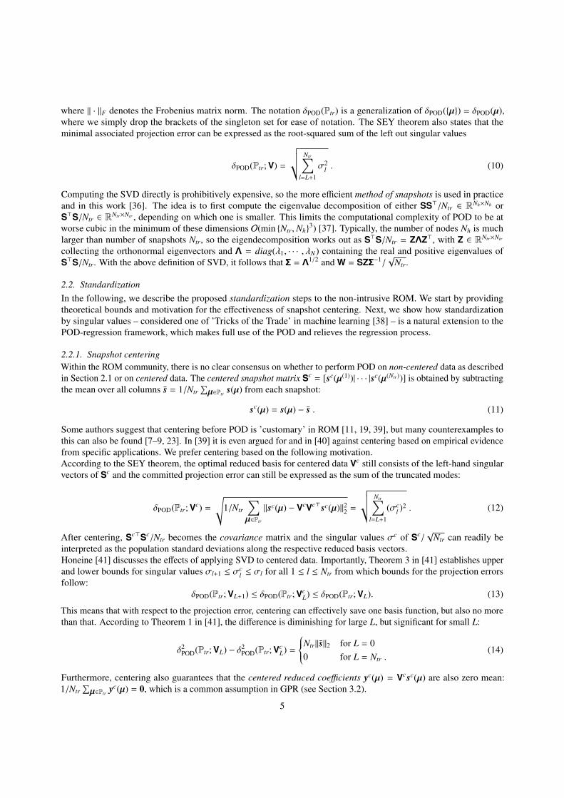
Figure 1: The figure illustrates the effect of the data preprocessing steps described in Section 2.2. For some parameter instance µ, s(µ) denotes thetwo-dimensional (Nh = 2) snapshot vector. Each element in the dataset is illustrated with a red dot, where ei is the i-th unit vector. Data is projectedon all available bases (L = Nh = 2). The final standardized data has zero mean and unit standard deviation along each basis vector, i.e., principaldirection. The shift and scale invariance serves to improve interpretability and model hyperparameter reusability not only for different principaldirections, but also across problems.

2.2.2. Coefficient standardizationAnother approach adopted in this work is coefficient standardization. The standardized reduced coefficients are obtainedby scaling the coefficients by the corresponding standard deviations:

ys(µ) = (Σc)−1yc(µ) . (15)

ys(µ) have a zero mean and unit variance for each of its L components and can thus be viewed as a multi-variate Z-scoreof the centered reduced coefficients. This achieves dataset standardization across different problems and allows to reusesimilar regression model architectures and learning processes, which are controlled by their hyperparameters. Normally,these must be found using tedious trial-and-error or an extensive and computationally expensive hyperparameter-tuning.Standardization allows to set tight bounds on the search-space or even reuse hyperparameters (see Section 3). Fig. 1helps illustrate the described transformation steps.

2.2.3. Parameter standardizationSimilar to the standardized reduced coefficients, we also introduce the standardized parameters as

µs = (µ − µ)/ ¯µ (16)

with the mean µ = 1/Ntr∑µ∈Ptr

µ and the standard deviation ¯µ =√

1/Ntr∑µ∈Ptr

(µ − µ)2. These again have zero meanand unit variance on any dataset following the same distribution as the training datset. This standardization step isbeneficial for regression tasks in problems, where different parameters are on different scales (see e.g. Section 5.3).Both RBF and GPR rely on distances in parameter space and would otherwise neglect the smaller parameters (seeSection 3.1 and Section 3.2). Similarly, ANNs show faster convergence with standardized inputs [42].

2.3. ErrorsWithin the POD-regression framework, errors are used to describe the quality of the reduced basis and the regressionmap. In Section 2.3.1, we show how a careful definition of these errors and their aggregation across multiple sampleslead to an intuitive and efficiently computable total error. In Section 2.3.2, we propose to standardize these errors, againconnecting the results to familiar statistical concepts, achieving better interpretability and comparability across datasets,as well as scale and translation invariances.

2.3.1. Absolute errorsThe absolute projection error δPOD has been already introduced in Equation (7) as the Euclidian distance between thesnapshot and its projection onto the reduced basis. The same holds with centering:

δPOD(µ; Vc) = ||s(µ) − sL(µ)||2 = ||sc(µ) − VcVc>sc(µ)||2 . (17)

6

vc1

vc2

(vc3)

sc scL

scL

δPOD

δREG

δPOD−REG

e1e2

e3

s

span(VcL=2 )

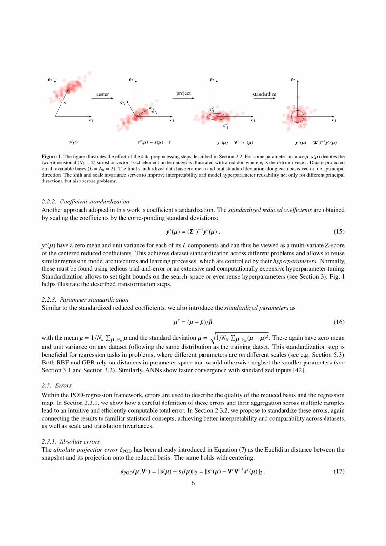
Figure 2: The total error δPOD-REG can be decomposed into two orthogonal components – the projection error δPOD perpendicular to the span ofcentered basis Vc and the regression error δREG belonging to the span. Illustration uses three degrees of freedom Nh = 3 and two reduced basisvectors L = 2.

Similarly, the absolute regression error δREG between the prediction sL(µ) and the projection sL(µ) is introduced todescribe how close the learned regression map πs approximates the observed regression map πs : µs 7→ ys:

δREG(µ; Vc, πs) = ||sL(µ) − sL(µ)||2 = ||scL(µ) − sc

L(µ)||2 =

= ||Vc yc(µ) − Vcyc(µ)||2 = ||yc(µ) − yc(µ)||2 =

= ||Σc (ys(µ) − ys(µ)) ||2 = ||Σc (πs(µs) − πs(µs)) ||2 .(18)

Lastly, the absolute total error δPOD-REG is introduced as the distance between the true and predicted solutions toquantify the performance of the whole non-intrusive ROM:

δPOD-REG(µ; Vc, πs) = ||s(µ) − sL(µ)||2 = ||sc(µ) − scL(µ)||2 . (19)

Fig. 2 illustrates these three types of errors. Additionally, it can be seen that the total error is composed of twoorthogonal components, namely the regression and projection errors:

δPOD-REG(µ)2 = δPOD(µ)2 + δREG(µ)2 . (20)

This can also be shown formally using the definition of the Euclidian vector norm ||a||22 = a>a and the fact that thepredictions already belong to the linear span of the reduced basis VcVc> sc

L = scL:

||sc − VcVc>sc||22+||VcVc>sc − scL||

22 =

= sc>sc − sc>VcVc> scL + sc

L> sc

L =

= sc>sc − sc> scL + sc

L> sc

L =

= ||sc−scL||

22

(21)

Lastly, we note that the equivalence in Equation (18) paired with with Equation (20) allows to compute both δREGand δPOD-REG in O(L) operations given that δPOD is regression independent and can be pre-computed once. In contrastto the naive approach via computing sc

L = Vc sc requiring O(NhL) operations due to matrix-vector multiplication, thepresented approach allows to efficiently use and monitor all errors during the training of the regression models.The corresponding aggregate projection, regression and total errors δ (P)∗ , ∗ ∈ POD,REG,POD-REG on any datasetP of cardinality N are defined via the root-mean-square error (RMSE):

δ∗ (P) :=√

1/N∑µ∈P δ∗ (µ)2 . (22)

7

This choice is motivated by the form of the SEY theorem and treats both physical and parameter dimensions equally.Hence, Equation (20) holds for both individual and aggregate errors.

2.3.2. Standardized errorsThe use of absolute errors makes it difficult to assess and interpret the performance of ROM, especially across differentdatasets. Thus we introduce the corresponding standardized projection, regression and total errors in the followingway:

ε∗ (P) :=δ∗ (P)√

1/Ntr∑µ∈Ptr

||s (µ) − s||2. (23)

The choice of the denominator is motivated by its relation to the standard deviation of the training set. Hence, εcan be interpreted as a multivariate extension of Z-score and describes the ratio between the Euclidian distanceof two vectors and the standard deviation of the particular dataset. Always naively predicting the mean vector sleads to 100% aggregated total error εPOD-REG(Ptr) = 1. Furthermore, the denominator can be related to POD, since1/Ntr

∑µ∈Ptr

||s (µ) − s||22 = 1/Ntr Tr(Sc>Sc) =∑Ntr

n=1 (σcn)2 . Consequentially, it is easy to relate the standardized

projection error to SEY and Equation (10):

ε2POD(Ptr; Vc

L) =

∑Ntrn=L+1 (σc

n)2∑Ntrn=1 (σc

n)2. (24)

This corresponds to a commonly used measure known as the relative information loss, which can be used to guide thechoice of number of bases L. Furthermore, ε is invariant to scaling and translation of snapshots and thus independentof the choice of units. This alleviates the need for designing dimensionless or normalized problems in order to interpretthe errors and altogether allows for a more data-driven approach to non-intrusive ROM. Finally, within the broaderclassification of existing error measures in machine learning, our definition of ε can be viewed as a multivariateextension of the root-relative-squared error, option 2 as classified by Botchkarev [43].

2.4. Time-resolved problems

In general, authors within ROM community approach time-resolved problems by treating time as a continuous parameter[7]. Wang et al. [23] point out two issues that arise using this approach. Firstly, for problems with many time steps Nt,the snapshot matrix becomes wide S ∈ RNh×Ntr Nt and the cost of the POD O

(min Nh,NtrNt

3)

becomes high even usingthe method of snapshots because the smallest dimension is increased significantly. Secondly, the regression model mustbe able to predict the solution at arbitrary time and parameter values. Thus it needs to learn both time and parameterdynamics. Several solutions to these problems have been proposed, mainly using two-level POD [1, 10, 19, 23, 31] oroperator inference [32].We propose an alternative method by relaxing the second requirement of needing to predict solutions at any arbitrarytime instance. Instead, we treat time in discrete levels, similar to physical space. This is inspired by typical numericalschemes, which also provide the solution at discrete spatial and temporal points, with any intermediate values beinginterpolated. This approach ensures that the snapshot matrix becomes taller not wider S ∈ RNhNt×Ntr , preserving thesmaller dimension Ntr and ensuring efficiency of the POD. Each resulting basis vector spans space and time, and as aconsequence the regression model must only account for parameter dynamics. This enables much simpler models andsignificantly reduces the effort of the fitting process.

3. Regression models

Within the non-intrusive ROM framework, the trained regression model is used to predict the reduced coefficients at anew parameter location using πs : µs 7→ ys. Note, that we standardize both the inputs and the outputs (see Section 2.2).As described in Section 1, any regression method can in principle be used. However, RBF regression is commonly useddue to its simplicity, but lately the more flexible GPR and ANN methods have been adopted in the ROM community[3, 7]. These three models are briefly described in the following.

8

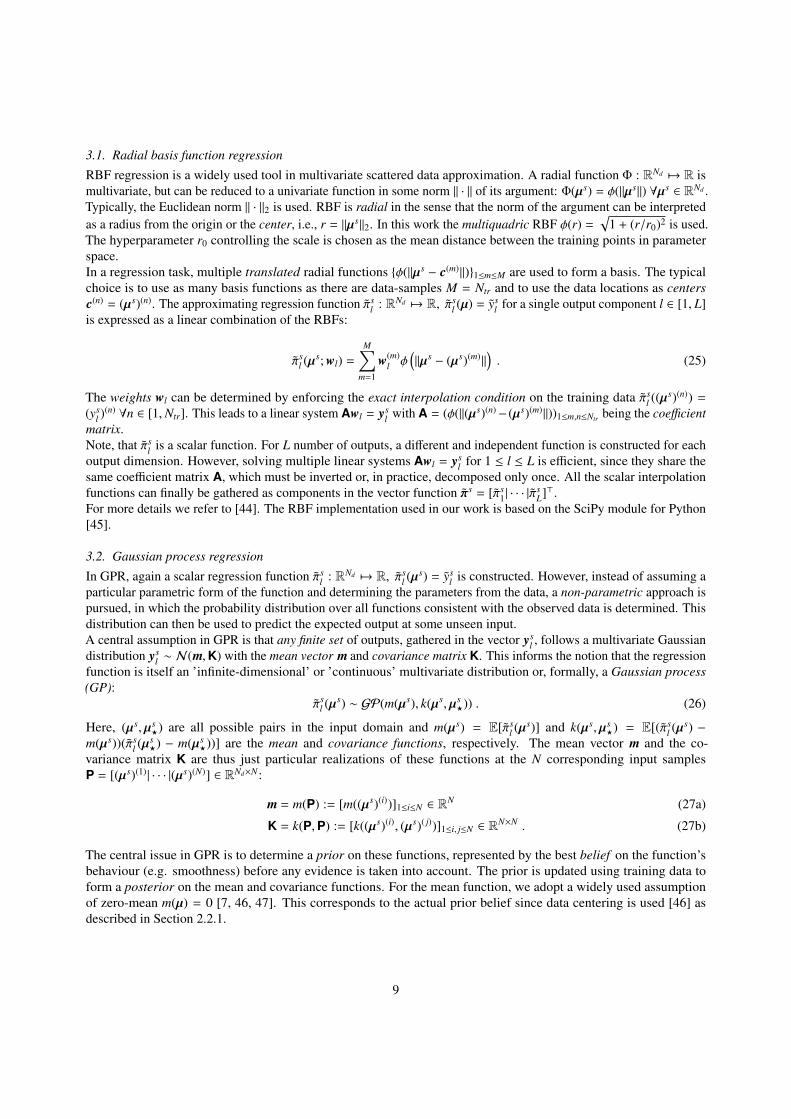
3.1. Radial basis function regression

RBF regression is a widely used tool in multivariate scattered data approximation. A radial function Φ : RNd 7→ R ismultivariate, but can be reduced to a univariate function in some norm || · || of its argument: Φ(µs) = φ(||µs||) ∀µs ∈ RNd .Typically, the Euclidean norm || · ||2 is used. RBF is radial in the sense that the norm of the argument can be interpretedas a radius from the origin or the center, i.e., r = ||µs||2. In this work the multiquadric RBF φ(r) =

√1 + (r/r0)2 is used.

The hyperparameter r0 controlling the scale is chosen as the mean distance between the training points in parameterspace.In a regression task, multiple translated radial functions φ(||µs − c(m)||)1≤m≤M are used to form a basis. The typicalchoice is to use as many basis functions as there are data-samples M = Ntr and to use the data locations as centersc(n) = (µs)(n). The approximating regression function πs

l : RNd 7→ R, πsl (µ) = ys

l for a single output component l ∈ [1, L]is expressed as a linear combination of the RBFs:

πsl (µs; wl) =

M∑m=1

w(m)l φ

(||µs − (µs)(m)||

). (25)

The weights wl can be determined by enforcing the exact interpolation condition on the training data πsl ((µ

s)(n)) =

(ysl )(n) ∀n ∈ [1,Ntr]. This leads to a linear system Awl = ys

l with A = (φ(||(µs)(n)− (µs)(m)||))1≤m,n≤Ntr being the coefficientmatrix.Note, that πs

l is a scalar function. For L number of outputs, a different and independent function is constructed for eachoutput dimension. However, solving multiple linear systems Awl = ys

l for 1 ≤ l ≤ L is efficient, since they share thesame coefficient matrix A, which must be inverted or, in practice, decomposed only once. All the scalar interpolationfunctions can finally be gathered as components in the vector function πs = [πs

1| · · · |πsL]>.

For more details we refer to [44]. The RBF implementation used in our work is based on the SciPy module for Python[45].

3.2. Gaussian process regression

In GPR, again a scalar regression function πsl : RNd 7→ R, πs

l (µs) = ysl is constructed. However, instead of assuming a

particular parametric form of the function and determining the parameters from the data, a non-parametric approach ispursued, in which the probability distribution over all functions consistent with the observed data is determined. Thisdistribution can then be used to predict the expected output at some unseen input.A central assumption in GPR is that any finite set of outputs, gathered in the vector ys

l , follows a multivariate Gaussiandistribution ys

l ∼ N(m,K) with the mean vector m and covariance matrix K. This informs the notion that the regressionfunction is itself an ’infinite-dimensional’ or ’continuous’ multivariate distribution or, formally, a Gaussian process(GP):

πsl (µs) ∼ GP(m(µs), k(µs,µs

?)) . (26)

Here, (µs,µs?) are all possible pairs in the input domain and m(µs) = E[πs

l (µs)] and k(µs,µs

?) = E[(πsl (µ

s) −m(µs))(πs

l (µs?) − m(µs

?))] are the mean and covariance functions, respectively. The mean vector m and the co-variance matrix K are thus just particular realizations of these functions at the N corresponding input samplesP = [(µs)(1)| · · · |(µs)(N)] ∈ RNd×N :

m = m(P) := [m((µs)(i))]1≤i≤N ∈ RN (27a)

K = k(P,P) := [k((µs)(i), (µs)( j))]1≤i, j≤N ∈ RN×N . (27b)

The central issue in GPR is to determine a prior on these functions, represented by the best belief on the function’sbehaviour (e.g. smoothness) before any evidence is taken into account. The prior is updated using training data toform a posterior on the mean and covariance functions. For the mean function, we adopt a widely used assumptionof zero-mean m(µ) = 0 [7, 46, 47]. This corresponds to the actual prior belief since data centering is used [46] asdescribed in Section 2.2.1.

9

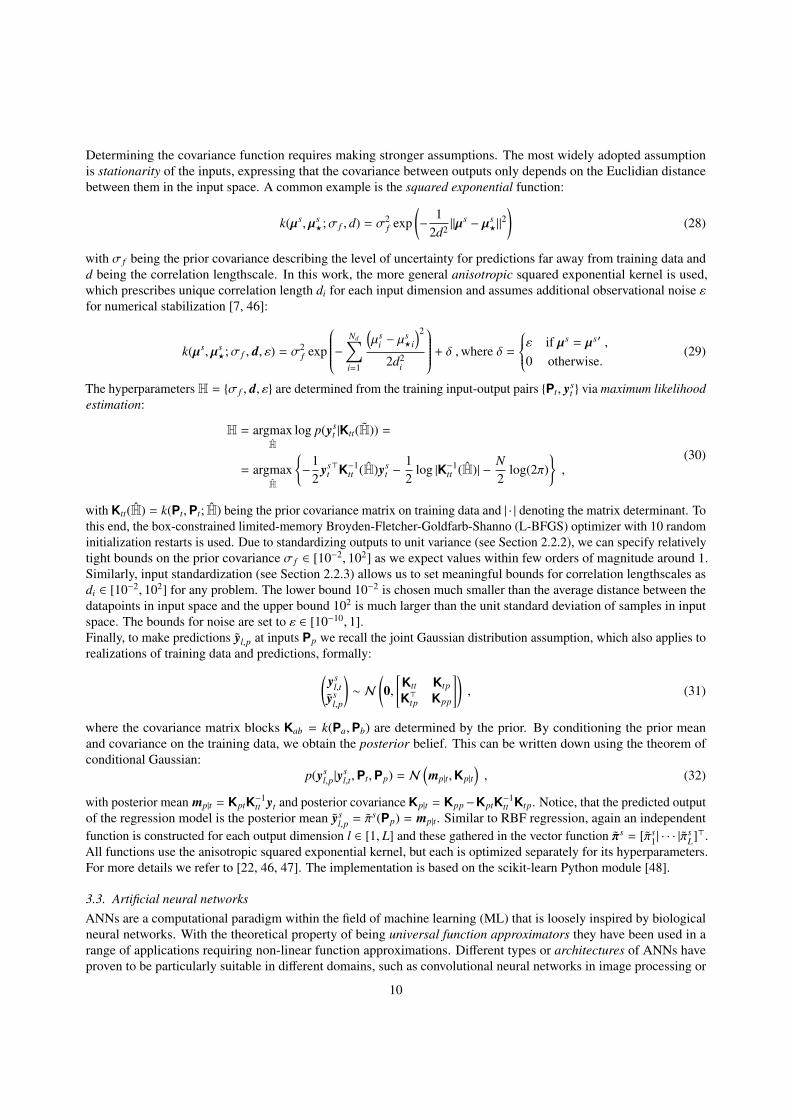
Determining the covariance function requires making stronger assumptions. The most widely adopted assumptionis stationarity of the inputs, expressing that the covariance between outputs only depends on the Euclidian distancebetween them in the input space. A common example is the squared exponential function:

k(µs,µs?;σ f , d) = σ2

f exp(−

12d2 ||µ

s − µs?||

2)

(28)

with σ f being the prior covariance describing the level of uncertainty for predictions far away from training data andd being the correlation lengthscale. In this work, the more general anisotropic squared exponential kernel is used,which prescribes unique correlation length di for each input dimension and assumes additional observational noise εfor numerical stabilization [7, 46]:

k(µs,µs?;σ f , d, ε) = σ2

f exp

− Nd∑i=1

(µs

i − µs?i

)2

2d2i

+ δ ,where δ =

ε if µs = µs′ ,

0 otherwise.(29)

The hyperparameters H = σ f , d, ε are determined from the training input-output pairs Pt, yst via maximum likelihood

estimation:

H = argmaxH

log p(yst |Ktt(H)) =

= argmaxH

−

12

yst>K−1

tt (H)yst −

12

log |K−1tt (H)| −

N2

log(2π),

(30)

with Ktt(H) = k(Pt,Pt; H) being the prior covariance matrix on training data and | · | denoting the matrix determinant. Tothis end, the box-constrained limited-memory Broyden-Fletcher-Goldfarb-Shanno (L-BFGS) optimizer with 10 randominitialization restarts is used. Due to standardizing outputs to unit variance (see Section 2.2.2), we can specify relativelytight bounds on the prior covariance σ f ∈ [10−2, 102] as we expect values within few orders of magnitude around 1.Similarly, input standardization (see Section 2.2.3) allows us to set meaningful bounds for correlation lengthscales asdi ∈ [10−2, 102] for any problem. The lower bound 10−2 is chosen much smaller than the average distance between thedatapoints in input space and the upper bound 102 is much larger than the unit standard deviation of samples in inputspace. The bounds for noise are set to ε ∈ [10−10, 1].Finally, to make predictions yl,p at inputs Pp we recall the joint Gaussian distribution assumption, which also applies torealizations of training data and predictions, formally:(

ysl,t

ysl,p

)∼ N

(0,

[Ktt Ktp

K>tp Kpp

]), (31)

where the covariance matrix blocks Kab = k(Pa,Pb) are determined by the prior. By conditioning the prior meanand covariance on the training data, we obtain the posterior belief. This can be written down using the theorem ofconditional Gaussian:

p(ysl,p|y

sl,t,Pt,Pp) = N

(mp|t,Kp|t

), (32)

with posterior mean mp|t = KptK−1tt yt and posterior covariance Kp|t = Kpp−KptK−1

tt Ktp. Notice, that the predicted outputof the regression model is the posterior mean ys

l,p = πs(Pp) = mp|t. Similar to RBF regression, again an independentfunction is constructed for each output dimension l ∈ [1, L] and these gathered in the vector function πs = [πs

1| · · · |πsL]>.

All functions use the anisotropic squared exponential kernel, but each is optimized separately for its hyperparameters.For more details we refer to [22, 46, 47]. The implementation is based on the scikit-learn Python module [48].

3.3. Artificial neural networksANNs are a computational paradigm within the field of machine learning (ML) that is loosely inspired by biologicalneural networks. With the theoretical property of being universal function approximators they have been used in arange of applications requiring non-linear function approximations. Different types or architectures of ANNs haveproven to be particularly suitable in different domains, such as convolutional neural networks in image processing or

10

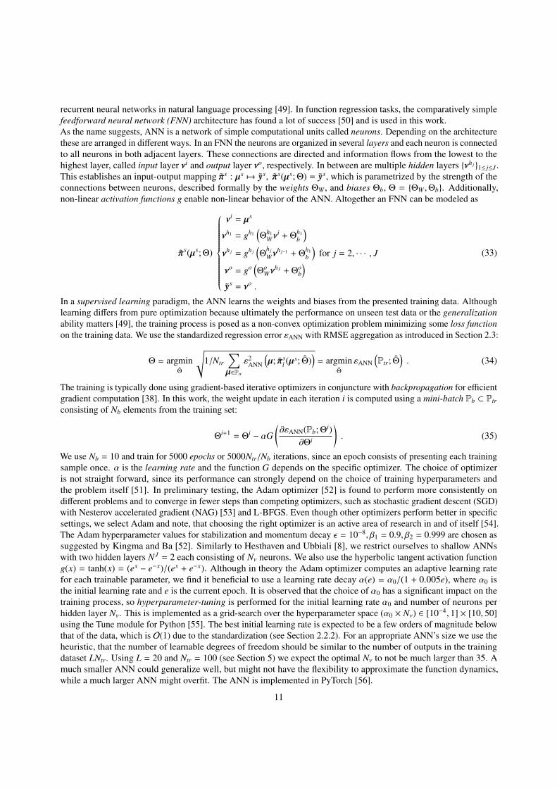
recurrent neural networks in natural language processing [49]. In function regression tasks, the comparatively simplefeedforward neural network (FNN) architecture has found a lot of success [50] and is used in this work.As the name suggests, ANN is a network of simple computational units called neurons. Depending on the architecturethese are arranged in different ways. In an FNN the neurons are organized in several layers and each neuron is connectedto all neurons in both adjacent layers. These connections are directed and information flows from the lowest to thehighest layer, called input layer νi and output layer νo, respectively. In between are multiple hidden layers νh j 1≤ j≤J .This establishes an input-output mapping πs : µs 7→ ys, πs(µs; Θ) = ys, which is parametrized by the strength of theconnections between neurons, described formally by the weights ΘW , and biases Θb, Θ = ΘW ,Θb. Additionally,non-linear activation functions g enable non-linear behavior of the ANN. Altogether an FNN can be modeled as

πs(µs; Θ)

νi = µs

νh1 = gh1(Θ

h1Wν

i + Θh1b

)νh j = gh j

(Θ

h j

Wνh j−1 + Θ

h1b

)for j = 2, · · · , J

νo = go(Θo

WνhJ + Θo

b

)ys = νo .

(33)

In a supervised learning paradigm, the ANN learns the weights and biases from the presented training data. Althoughlearning differs from pure optimization because ultimately the performance on unseen test data or the generalizationability matters [49], the training process is posed as a non-convex optimization problem minimizing some loss functionon the training data. We use the standardized regression error εANN with RMSE aggregation as introduced in Section 2.3:

Θ = argminΘ

√1/Ntr

∑µ∈Ptr

ε2ANN

(µ; πs

l (µs; Θ))

= argminΘ

εANN

(Ptr; Θ

). (34)

The training is typically done using gradient-based iterative optimizers in conjuncture with backpropagation for efficientgradient computation [38]. In this work, the weight update in each iteration i is computed using a mini-batch Pb ⊂ Ptr

consisting of Nb elements from the training set:

Θi+1 = Θi − αG(∂εANN(Pb; Θi)

∂Θi

). (35)

We use Nb = 10 and train for 5000 epochs or 5000Ntr/Nb iterations, since an epoch consists of presenting each trainingsample once. α is the learning rate and the function G depends on the specific optimizer. The choice of optimizeris not straight forward, since its performance can strongly depend on the choice of training hyperparameters andthe problem itself [51]. In preliminary testing, the Adam optimizer [52] is found to perform more consistently ondifferent problems and to converge in fewer steps than competing optimizers, such as stochastic gradient descent (SGD)with Nesterov accelerated gradient (NAG) [53] and L-BFGS. Even though other optimizers perform better in specificsettings, we select Adam and note, that choosing the right optimizer is an active area of research in and of itself [54].The Adam hyperparameter values for stabilization and momentum decay ε = 10−8, β1 = 0.9, β2 = 0.999 are chosen assuggested by Kingma and Ba [52]. Similarly to Hesthaven and Ubbiali [8], we restrict ourselves to shallow ANNswith two hidden layers N J = 2 each consisting of Nν neurons. We also use the hyperbolic tangent activation functiong(x) = tanh(x) = (ex − e−x)/(ex + e−x). Although in theory the Adam optimizer computes an adaptive learning ratefor each trainable parameter, we find it beneficial to use a learning rate decay α(e) = α0/(1 + 0.005e), where α0 isthe initial learning rate and e is the current epoch. It is observed that the choice of α0 has a significant impact on thetraining process, so hyperparameter-tuning is performed for the initial learning rate α0 and number of neurons perhidden layer Nν. This is implemented as a grid-search over the hyperparameter space (α0 × Nν) ∈ [10−4, 1] × [10, 50]using the Tune module for Python [55]. The best initial learning rate is expected to be a few orders of magnitude belowthat of the data, which is O(1) due to the standardization (see Section 2.2.2). For an appropriate ANN’s size we use theheuristic, that the number of learnable degrees of freedom should be similar to the number of outputs in the trainingdataset LNtr. Using L = 20 and Ntr = 100 (see Section 5) we expect the optimal Nν to not be much larger than 35. Amuch smaller ANN could generalize well, but might not have the flexibility to approximate the function dynamics,while a much larger ANN might overfit. The ANN is implemented in PyTorch [56].

11

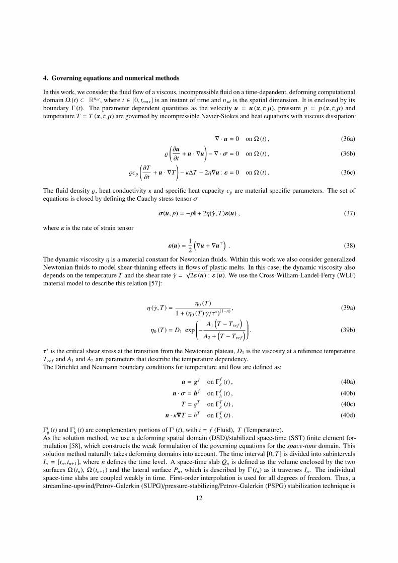
4. Governing equations and numerical methods

In this work, we consider the fluid flow of a viscous, incompressible fluid on a time-dependent, deforming computationaldomain Ω (t) ⊂ Rnsd , where t ∈ [0, tmax] is an instant of time and nsd is the spatial dimension. It is enclosed by itsboundary Γ (t). The parameter dependent quantities as the velocity u = u (x, t;µ), pressure p = p (x, t;µ) andtemperature T = T (x, t;µ) are governed by incompressible Navier-Stokes and heat equations with viscous dissipation:

∇ · u = 0 on Ω (t) , (36a)

%

(∂u∂t

+ u · ∇u)− ∇ · σ = 0 on Ω (t) , (36b)

%cp

(∂T∂t

+ u · ∇T)− κ∆T − 2η∇u : ε = 0 on Ω (t) . (36c)

The fluid density %, heat conductivity κ and specific heat capacity cp are material specific parameters. The set ofequations is closed by defining the Cauchy stress tensor σ

σ(u, p) = −pI + 2η(γ,T )ε(u) , (37)

where ε is the rate of strain tensor

ε(u) =12

(∇u + ∇u>

). (38)

The dynamic viscosity η is a material constant for Newtonian fluids. Within this work we also consider generalizedNewtonian fluids to model shear-thinning effects in flows of plastic melts. In this case, the dynamic viscosity alsodepends on the temperature T and the shear rate γ =

√2ε (u) : ε (u). We use the Cross-William-Landel-Ferry (WLF)

material model to describe this relation [57]:

η (γ,T ) =η0 (T )

1 + (η0 (T ) γ/τ∗)(1−n) , (39a)

η0 (T ) = D1 exp

− A1

(T − Tre f

)A2 +

(T − Tre f

) . (39b)

τ∗ is the critical shear stress at the transition from the Newtonian plateau, D1 is the viscosity at a reference temperatureTre f and A1 and A2 are parameters that describe the temperature dependency.The Dirichlet and Neumann boundary conditions for temperature and flow are defined as:

u = g f on Γfg (t) , (40a)

n · σ = h f on Γfh (t) , (40b)

T = gT on ΓTg (t) , (40c)

n · κ∇T = hT on ΓTh (t) . (40d)

Γig (t) and Γi

h (t) are complementary portions of Γi (t), with i = f (Fluid), T (Temperature).As the solution method, we use a deforming spatial domain (DSD)/stabilized space-time (SST) finite element for-mulation [58], which constructs the weak formulation of the governing equations for the space-time domain. Thissolution method naturally takes deforming domains into account. The time interval [0,T ] is divided into subintervalsIn = [tn, tn+1], where n defines the time level. A space-time slab Qn is defined as the volume enclosed by the twosurfaces Ω (tn), Ω (tn+1) and the lateral surface Pn, which is described by Γ (tn) as it traverses In. The individualspace-time slabs are coupled weakly in time. First-order interpolation is used for all degrees of freedom. Thus, astreamline-upwind/Petrov-Galerkin (SUPG)/pressure-stabilizing/Petrov-Galerkin (PSPG) stabilization technique is

12

used to fulfill the Ladyzhenskaya-Babuška-Brezzi (LBB) condition [59]. For a more detailed description of the solutionmethod, we refer to [33, 58, 60].For the selection of snapshots for the ROM we have to take into account that two spatial solution fields exist at adiscrete time instance tn+1: the upper field of the space-time slabs at In and the lower field of the space-time slabs atIn+1. These fields do not necessarily match exactly since they are only coupled weakly. However, we are only interestedin the solution at the discrete time level. Thus, we only use the upper solution field of In. As described in Section 2,an advantage of non-intrusive ROM is that the data can stem from any discretization method or even experimentalobservations.

5. Numerical results

In this section, we apply our standardized non-intrusive ROM to three different fluid flow problems of increasingcomplexity. We start with a validation problem in Section 5.1, then add time dependency, parametric material properties,and temperature dependence in Section 5.2. Finally, in Section 5.3, we move to our main use-case – the twin-screwextruder. Across all problems and quantities of interest, we compare the performance of the three regression models, aswell as the results of ANN’s hyperparameter tuning.

5.1. Skewed lid-driven cavity

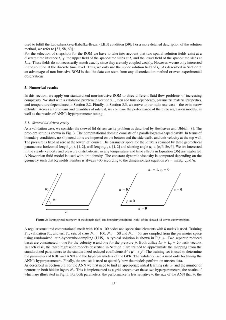
As a validation case, we consider the skewed lid-driven cavity problem as described by Hesthaven and Ubbiali [8]. Theproblem setup is shown in Fig. 3. The computational domain consists of a parallelogram-shaped cavity. In terms ofboundary conditions, no-slip conditions are imposed on the bottom and the side walls, and unit velocity at the top wall.The pressure is fixed at zero at the lower left corner. The parameter space for the ROM is spanned by three geometricalparameters: horizontal length µ1 ∈ [1, 2], wall length µ2 ∈ [1, 2] and slanting angle µ3 ∈ [π/6, 5π/6]. We are interestedin the steady velocity and pressure distributions, so any temperature and time effects in Equation (36) are neglected.A Newtonian fluid model is used with unit density. The constant dynamic viscosity is computed depending on thegeometry such that Reynolds number is always 400 according to the dimensionless equation Re = maxµ1, µ2/η.

µ3

µ1

µ2 u = 0

ux = 1, uy = 0

u = 0

u = 0

p = 0

Figure 3: Parametrized geometry of the domain (left) and boundary conditions (right) of the skewed lid-driven cavity problem.

A regular structured computational mesh with 100 × 100 nodes and space-time elements with 8-nodes is used. TrainingPtr, validation Pva and test Pte sets of sizes Ntr = 100, Nva = 50 and Nte = 50, are sampled from the parameter-spaceusing randomized latin-hypercube-sampling (LHS). A typical solution is shown in Fig. 4. Two separate reducedbases are constructed – one for the velocity u and one for the pressure p. Both utilize Lu = Lp = 20 basis vectors.In each case, the three regression models described in Section 3 are trained to approximate the mapping from thestandardized parameters to the standardized reduced coefficients πs : µs 7→ ys. The training set is used to determinethe parameters of RBF and ANN and the hyperparameters of the GPR. The validation set is used only for tuning theANN’s hyperparameters. Finally, the test set is used to quantify how the models perform on unseen data.As described in Section 3.3, for the ANN we first need to find an appropriate initial learning rate α0 and the number ofneurons in both hidden layers Nν. This is implemented as a grid-search over these two hyperparameters, the results ofwhich are illustrated in Fig. 5. For both parameters, the performance is less sensitive to the size of the ANN than to the

13

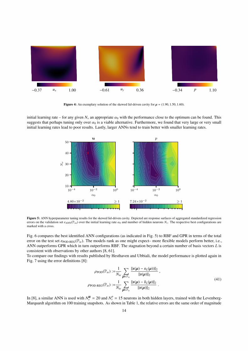
−0.37 ux 1.00 −0.61 uy 0.36 −0.34 p 1.10

Figure 4: An exemplary solution of the skewed lid-driven cavity for µ = (1.90, 1.50, 1.60).

initial learning rate – for any given Nν an appropriate α0 with the performance close to the optimum can be found. Thissuggests that perhaps tuning only over α0 is a viable alternative. Furthermore, we found that very large or very smallinitial learning rates lead to poor results. Lastly, larger ANNs tend to train better with smaller learning rates.

10−4 10−2 100

α0

10

20

30

40

50

Nν

u

10−4 10−2 100

α0

p

4.80×10−2 ≥ 1 7.24×10−2 ≥ 1

Figure 5: ANN hyperparameter tuning results for the skewed lid-driven cavity. Depicted are response surfaces of aggregated standardized regressionerrors on the validation set εANN(Pva) over the initial learning rate α0 and number of hidden neurons Nν. The respective best configurations aremarked with a cross.

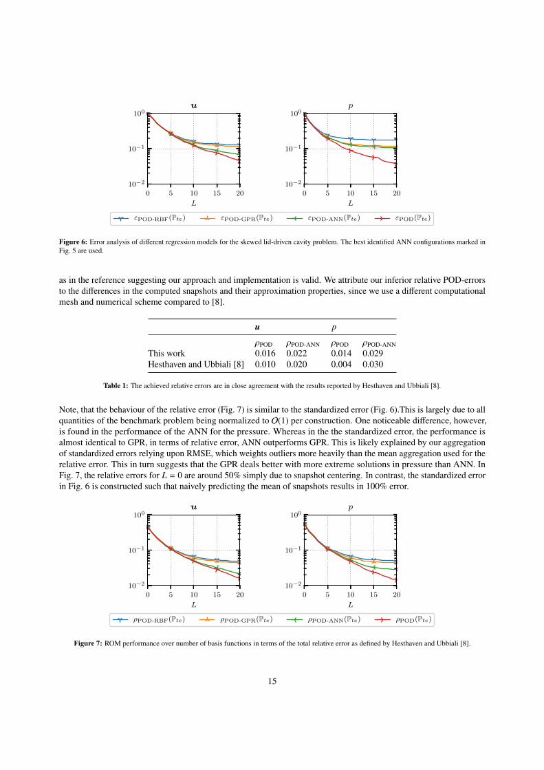
Fig. 6 compares the best identified ANN configurations (as indicated in Fig. 5) to RBF and GPR in terms of the totalerror on the test set εPOD-REG(Pte). The models rank as one might expect– more flexible models perform better, i.e.,ANN outperforms GPR which in turn outperforms RBF. The stagnation beyond a certain number of basis vectors L isconsistent with observations by other authors [8, 61].To compare our findings with results published by Hesthaven and Ubbiali, the model performance is plotted again inFig. 7 using the error definitions [8]:

ρPOD(Pte) :=1

Nte

∑µ∈Pte

||s(µ) − sL(µ))||2||s(µ)||2

,

ρPOD-REG(Pte) :=1

Nte

∑µ∈Pte

||s(µ) − sL(µ)||2||s(µ)||2

.

(41)

In [8], a similar ANN is used with Nuν = 20 and N p

ν = 15 neurons in both hidden layers, trained with the Levenberg-Marquardt algorithm on 100 training snapshots. As shown in Table 1, the relative errors are the same order of magnitude

14

0 5 10 15 20

L

10−2

10−1

100u

0 5 10 15 20

L

10−2

10−1

100p

εPOD-RBF(Pte) εPOD-GPR(Pte) εPOD-ANN(Pte) εPOD(Pte)

Figure 6: Error analysis of different regression models for the skewed lid-driven cavity problem. The best identified ANN configurations marked inFig. 5 are used.

as in the reference suggesting our approach and implementation is valid. We attribute our inferior relative POD-errorsto the differences in the computed snapshots and their approximation properties, since we use a different computationalmesh and numerical scheme compared to [8].

u p

ρPOD ρPOD-ANN ρPOD ρPOD-ANNThis work 0.016 0.022 0.014 0.029Hesthaven and Ubbiali [8] 0.010 0.020 0.004 0.030

Table 1: The achieved relative errors are in close agreement with the results reported by Hesthaven and Ubbiali [8].

Note, that the behaviour of the relative error (Fig. 7) is similar to the standardized error (Fig. 6).This is largely due to allquantities of the benchmark problem being normalized to O(1) per construction. One noticeable difference, however,is found in the performance of the ANN for the pressure. Whereas in the the standardized error, the performance isalmost identical to GPR, in terms of relative error, ANN outperforms GPR. This is likely explained by our aggregationof standardized errors relying upon RMSE, which weights outliers more heavily than the mean aggregation used for therelative error. This in turn suggests that the GPR deals better with more extreme solutions in pressure than ANN. InFig. 7, the relative errors for L = 0 are around 50% simply due to snapshot centering. In contrast, the standardized errorin Fig. 6 is constructed such that naively predicting the mean of snapshots results in 100% error.

0 5 10 15 20

L

10−2

10−1

100u

0 5 10 15 20

L

10−2

10−1

100p

ρPOD-RBF(Pte) ρPOD-GPR(Pte) ρPOD-ANN(Pte) ρPOD(Pte)

Figure 7: ROM performance over number of basis functions in terms of the total relative error as defined by Hesthaven and Ubbiali [8].

15

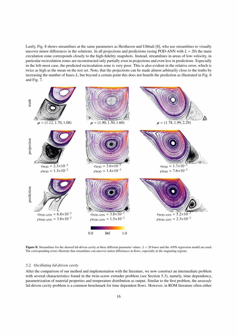
Lastly, Fig. 8 shows streamlines at the same parameters as Hesthaven and Ubbiali [8], who use streamlines to visuallyuncover minor differences in the solutions. In all projections and predictions (using POD-ANN with L = 20) the maincirculation zone corresponds closely to the high-fidelity snapshots. Instead, streamlines in areas of low-velocity, inparticular recirculation zones are reconstructed only partially even in projections and even less in predictions. Especiallyin the left-most case, the predicted recirculation zone is very poor. This is also evident in the relative error, which istwice as high as the mean on the test set. Note, that the projections can be made almost arbitrarily close to the truths byincreasing the number of bases L, but beyond a certain point this does not benefit the prediction as illustrated in Fig. 6and Fig. 7.

trut

h

µ = (1.12, 1.70, 1.08) µ = (1.90, 1.50, 1.60) µ = (1.78, 1.99, 2.29)

proj

ectio

n

εPOD = 2.3×10−2 εPOD = 3.6×10−2 εPOD = 1.7×10−2

ρPOD = 1.3×10−2 ρPOD = 1.4×10−3 ρPOD = 7.6×10−3

pred

ictio

n

εPOD-ANN = 6.8×10−2 εPOD-ANN = 3.8×10−2 εPOD-ANN = 5.2×10−2

ρPOD-ANN = 3.8×10−2 ρPOD-ANN = 1.5×10−2 ρPOD-ANN = 2.3×10−2

0.0 ||u|| 1.0

Figure 8: Streamlines for the skewed lid-driven cavity at three different parameter values. L = 20 bases and the ANN regression model are used.The corresponding errors illustrate that streamlines can uncover minor differences in flows, especially in the stagnating regions.

5.2. Oscillating lid-driven cavity

After the comparison of our method and implementation with the literature, we now construct an intermediate problemwith several characteristics found in the twin-screw extruder problem (see Section 5.3), namely, time dependency,parametrization of material properties and temperature distribution as output. Similar to the first problem, the unsteadylid-driven cavity problem is a common benchmark for time dependent flows. However, in ROM literature often either

16

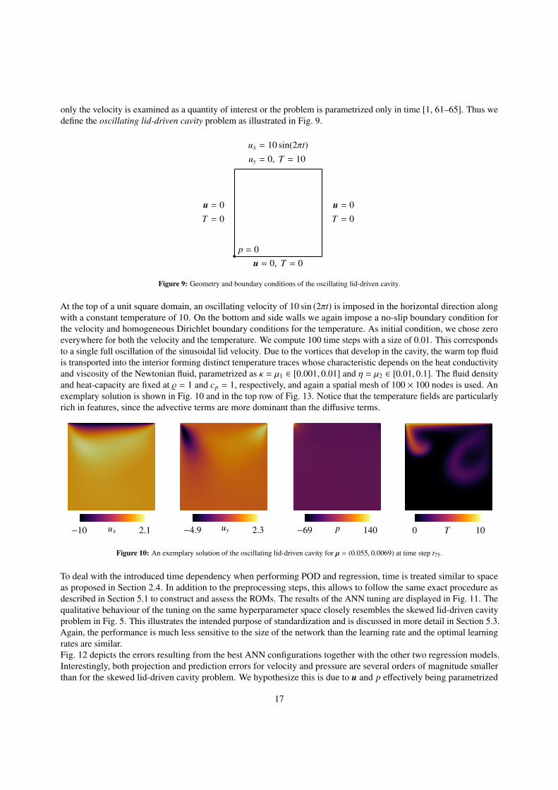
only the velocity is examined as a quantity of interest or the problem is parametrized only in time [1, 61–65]. Thus wedefine the oscillating lid-driven cavity problem as illustrated in Fig. 9.

u = 0T = 0

ux = 10 sin(2πt)uy = 0, T = 10

u = 0T = 0

u = 0, T = 0p = 0

Figure 9: Geometry and boundary conditions of the oscillating lid-driven cavity.

At the top of a unit square domain, an oscillating velocity of 10 sin (2πt) is imposed in the horizontal direction alongwith a constant temperature of 10. On the bottom and side walls we again impose a no-slip boundary condition forthe velocity and homogeneous Dirichlet boundary conditions for the temperature. As initial condition, we chose zeroeverywhere for both the velocity and the temperature. We compute 100 time steps with a size of 0.01. This correspondsto a single full oscillation of the sinusoidal lid velocity. Due to the vortices that develop in the cavity, the warm top fluidis transported into the interior forming distinct temperature traces whose characteristic depends on the heat conductivityand viscosity of the Newtonian fluid, parametrized as κ = µ1 ∈ [0.001, 0.01] and η = µ2 ∈ [0.01, 0.1]. The fluid densityand heat-capacity are fixed at % = 1 and cp = 1, respectively, and again a spatial mesh of 100 × 100 nodes is used. Anexemplary solution is shown in Fig. 10 and in the top row of Fig. 13. Notice that the temperature fields are particularlyrich in features, since the advective terms are more dominant than the diffusive terms.

−10 ux 2.1 −4.9 uy 2.3 −69 p 140 0 T 10

Figure 10: An exemplary solution of the oscillating lid-driven cavity for µ = (0.055, 0.0069) at time step t75.

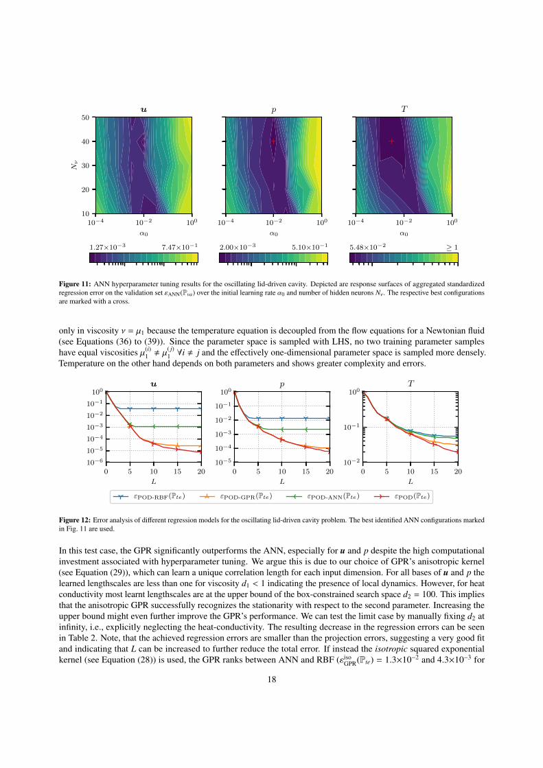
To deal with the introduced time dependency when performing POD and regression, time is treated similar to spaceas proposed in Section 2.4. In addition to the preprocessing steps, this allows to follow the same exact procedure asdescribed in Section 5.1 to construct and assess the ROMs. The results of the ANN tuning are displayed in Fig. 11. Thequalitative behaviour of the tuning on the same hyperparameter space closely resembles the skewed lid-driven cavityproblem in Fig. 5. This illustrates the intended purpose of standardization and is discussed in more detail in Section 5.3.Again, the performance is much less sensitive to the size of the network than the learning rate and the optimal learningrates are similar.Fig. 12 depicts the errors resulting from the best ANN configurations together with the other two regression models.Interestingly, both projection and prediction errors for velocity and pressure are several orders of magnitude smallerthan for the skewed lid-driven cavity problem. We hypothesize this is due to u and p effectively being parametrized

17

10−4 10−2 100

α0

10

20

30

40

50

Nν

u

10−4 10−2 100

α0

p

10−4 10−2 100

α0

T

1.27×10−3 7.47×10−1 2.00×10−3 5.10×10−1 5.48×10−2 ≥ 1

Figure 11: ANN hyperparameter tuning results for the oscillating lid-driven cavity. Depicted are response surfaces of aggregated standardizedregression error on the validation set εANN(Pva) over the initial learning rate α0 and number of hidden neurons Nν. The respective best configurationsare marked with a cross.

only in viscosity ν = µ1 because the temperature equation is decoupled from the flow equations for a Newtonian fluid(see Equations (36) to (39)). Since the parameter space is sampled with LHS, no two training parameter sampleshave equal viscosities µ(i)

1 , µ( j)1 ∀i , j and the effectively one-dimensional parameter space is sampled more densely.

Temperature on the other hand depends on both parameters and shows greater complexity and errors.

0 5 10 15 20

L

10−6

10−5

10−4

10−3

10−2

10−1

100u

0 5 10 15 20

L

10−5

10−4

10−3

10−2

10−1

100p

0 5 10 15 20

L

10−2

10−1

100T

εPOD-RBF(Pte) εPOD-GPR(Pte) εPOD-ANN(Pte) εPOD(Pte)

Figure 12: Error analysis of different regression models for the oscillating lid-driven cavity problem. The best identified ANN configurations markedin Fig. 11 are used.

In this test case, the GPR significantly outperforms the ANN, especially for u and p despite the high computationalinvestment associated with hyperparameter tuning. We argue this is due to our choice of GPR’s anisotropic kernel(see Equation (29)), which can learn a unique correlation length for each input dimension. For all bases of u and p thelearned lengthscales are less than one for viscosity d1 < 1 indicating the presence of local dynamics. However, for heatconductivity most learnt lengthscales are at the upper bound of the box-constrained search space d2 = 100. This impliesthat the anisotropic GPR successfully recognizes the stationarity with respect to the second parameter. Increasing theupper bound might even further improve the GPR’s performance. We can test the limit case by manually fixing d2 atinfinity, i.e., explicitly neglecting the heat-conductivity. The resulting decrease in the regression errors can be seenin Table 2. Note, that the achieved regression errors are smaller than the projection errors, suggesting a very good fitand indicating that L can be increased to further reduce the total error. If instead the isotropic squared exponentialkernel (see Equation (28)) is used, the GPR ranks between ANN and RBF (εiso

GPR(Pte) = 1.3×10−2 and 4.3×10−3 for

18

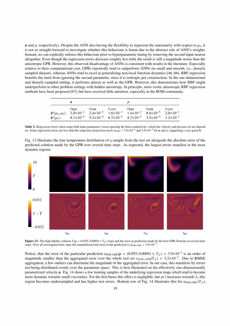
u and p, respectively). Despite the ANN also having the flexibility to represent the stationarity with respect to µ2, itis not as straight-forward to investigate whether this behaviour is learnt due to the abstract role of ANN’s weights.Instead, we can explicitly enforce this behaviour prior to hyperparameter tuning by removing the second input neuronaltogether. Even though the regression errors decrease roughly five-fold, the result is still a magnitude worse than theanisotropic GPR. However, this observed disadvantage of ANNs is consistent with results in the literature. Especiallyrelative to their computational cost, GPRs reportedly tend to outperform ANNs on small and smooth, i.e., denselysampled datasets, whereas ANNs tend to excel at generalizing non-local function dynamics [46, 66]. RBF regressionbenefits the most from ignoring the second parameter, since it is isotropic per construction. In the one-dimensionaland densely-sampled setting, it performs almost as well as the GPR. However, this demonstrates how RBF mightunderperform in other problem settings with hidden anisotropy. In principle, more exotic anisotropic RBF regressionmethods have been proposed [67], but have received little attention, especially in the ROM community.

u p

εRBF εGPR εANN εRBF εGPR εANNπs(µ1, µ2) 3.8×10−2 2.4×10−5 1.6×10−3 1.4×10−2 8.6×10−5 2.0×10−3

πs(µ1) 8.1×10−6 5.3×10−6 6.7×10−4 4.7×10−5 3.5×10−5 1.2×10−3

Table 2: Regression errors when using both input parameters versus ignoring the heat-conductivity, which the velocity and pressure do not dependon. Some regression errors are less than the respective projection errors εPOD = 7.8×10−6 and 5.9×10−5 for u and p, suggesting a very good fit.

Fig. 13 illustrates the true temperature distribution of a sample from the test set alongside the absolute error of thepredicted solution made by the GPR over several time steps. As expected, the largest errors manifest in the mostdynamic regions.

0

T

10

−0.032

T − T

0.032

t50 t60 t70 t80

Figure 13: The high-fidelity solution T (µ = (0.055, 0.0069) ∈ Pte) (top) and the error in prediction made by the best GPR (bottom) at several timesteps. Over all investigated time steps the standardized total error in the prediction is εPOD-GPR = 3.9×10−3.

Notice, that the error of the particular prediction εPOD-GPR(µ = (0.055, 0.0069) ∈ Pte) = 3.9×10−3 is an order ofmagnitude smaller than the aggregated error over the whole test set εPOD−GPR(Pte) = 3.2×10−2. Due to RMSEaggregation, a few outliers can determine the magnitude of the aggregated error. In our case, this manifests by errorsnot being distributed evenly over the parameter space. This is best illustrated on the effectively one-dimensionallyparametrized velocity u. Fig. 14 shows a few training samples of the underlying regression maps which tend to becomemore dynamic towards small viscosities. For the first bases this effect is negligible, but as l increases towards L, thisregion becomes undersampled and has higher test errors. Bottom row of Fig. 14 illustrates this for εPOD-GPR (Pte),

19

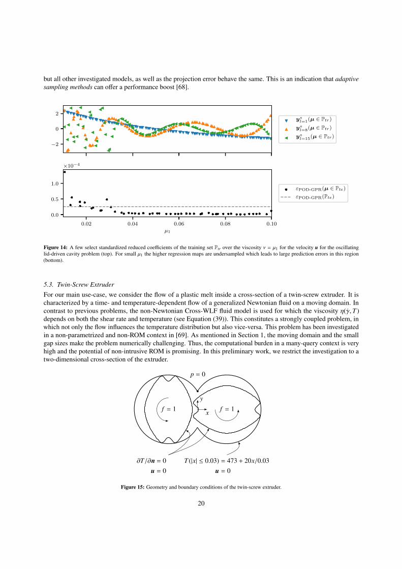
but all other investigated models, as well as the projection error behave the same. This is an indication that adaptivesampling methods can offer a performance boost [68].

−2

0

2ysl=1(µ ∈ Ptr)

ysl=8(µ ∈ Ptr)

ysl=15(µ ∈ Ptr)

0.02 0.04 0.06 0.08 0.10

µ1

0.0

0.5

1.0

×10−4

εPOD-GPR(µ ∈ Pte)εPOD-GPR(Pte)

Figure 14: A few select standardized reduced coefficients of the training set Ptr over the viscosity ν = µ1 for the velocity u for the oscillatinglid-driven cavity problem (top). For small µ1 the higher regression maps are undersampled which leads to large prediction errors in this region(bottom).

5.3. Twin-Screw Extruder

For our main use-case, we consider the flow of a plastic melt inside a cross-section of a twin-screw extruder. It ischaracterized by a time- and temperature-dependent flow of a generalized Newtonian fluid on a moving domain. Incontrast to previous problems, the non-Newtonian Cross-WLF fluid model is used for which the viscosity η(γ,T )depends on both the shear rate and temperature (see Equation (39)). This constitutes a strongly coupled problem, inwhich not only the flow influences the temperature distribution but also vice-versa. This problem has been investigatedin a non-parametrized and non-ROM context in [69]. As mentioned in Section 1, the moving domain and the smallgap sizes make the problem numerically challenging. Thus, the computational burden in a many-query context is veryhigh and the potential of non-intrusive ROM is promising. In this preliminary work, we restrict the investigation to atwo-dimensional cross-section of the extruder.

p = 0

x

y

f = 1 f = 1

T (|x| ≤ 0.03) = 473 + 20x/0.03u = 0

∂T/∂n = 0u = 0

Figure 15: Geometry and boundary conditions of the twin-screw extruder.

20

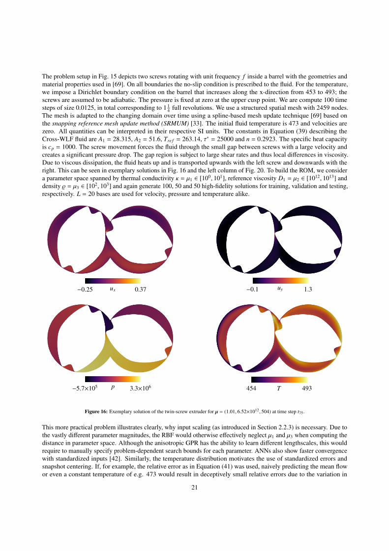
The problem setup in Fig. 15 depicts two screws rotating with unit frequency f inside a barrel with the geometries andmaterial properties used in [69]. On all boundaries the no-slip condition is prescribed to the fluid. For the temperature,we impose a Dirichlet boundary condition on the barrel that increases along the x-direction from 453 to 493; thescrews are assumed to be adiabatic. The pressure is fixed at zero at the upper cusp point. We are compute 100 timesteps of size 0.0125, in total corresponding to 1 1

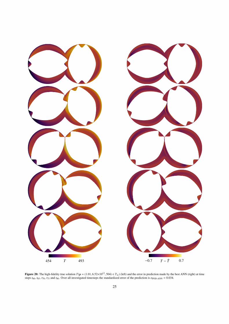
4 full revolutions. We use a structured spatial mesh with 2459 nodes.The mesh is adapted to the changing domain over time using a spline-based mesh update technique [69] based onthe snapping reference mesh update method (SRMUM) [33]. The initial fluid temperature is 473 and velocities arezero. All quantities can be interpreted in their respective SI units. The constants in Equation (39) describing theCross-WLF fluid are A1 = 28.315, A2 = 51.6, Tre f = 263.14, τ∗ = 25000 and n = 0.2923. The specific heat capacityis cp = 1000. The screw movement forces the fluid through the small gap between screws with a large velocity andcreates a significant pressure drop. The gap region is subject to large shear rates and thus local differences in viscosity.Due to viscous dissipation, the fluid heats up and is transported upwards with the left screw and downwards with theright. This can be seen in exemplary solutions in Fig. 16 and the left column of Fig. 20. To build the ROM, we considera parameter space spanned by thermal conductivity κ = µ1 ∈ [100, 101], reference viscosity D1 = µ2 ∈ [1012, 1013] anddensity % = µ3 ∈ [102, 103] and again generate 100, 50 and 50 high-fidelity solutions for training, validation and testing,respectively. L = 20 bases are used for velocity, pressure and temperature alike.

−0.25 ux 0.37 −0.1 uy 1.3

−5.7×105 p 3.3×106 454 T 493

Figure 16: Exemplary solution of the twin-screw extruder for µ = (1.01, 6.52×1012, 504) at time step t75.

This more practical problem illustrates clearly, why input scaling (as introduced in Section 2.2.3) is necessary. Due tothe vastly different parameter magnitudes, the RBF would otherwise effectively neglect µ1 and µ3 when computing thedistance in parameter space. Although the anisotropic GPR has the ability to learn different lengthscales, this wouldrequire to manually specify problem-dependent search bounds for each parameter. ANNs also show faster convergencewith standardized inputs [42]. Similarly, the temperature distribution motivates the use of standardized errors andsnapshot centering. If, for example, the relative error as in Equation (41) was used, naively predicting the mean flowor even a constant temperature of e.g. 473 would result in deceptively small relative errors due to the variation in

21

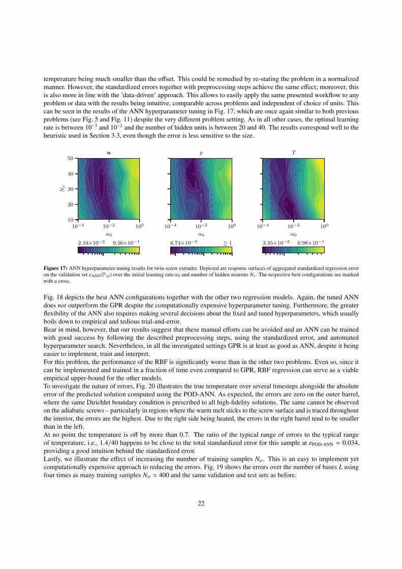
temperature being much smaller than the offset. This could be remedied by re-stating the problem in a normalizedmanner. However, the standardized errors together with preprocessing steps achieve the same effect; moreover, thisis also more in line with the ’data-driven’ approach. This allows to easily apply the same presented workflow to anyproblem or data with the results being intuitive, comparable across problems and independent of choice of units. Thiscan be seen in the results of the ANN hyperparameter tuning in Fig. 17, which are once again similar to both previousproblems (see Fig. 5 and Fig. 11) despite the very different problem setting. As in all other cases, the optimal learningrate is between 10−3 and 10−2 and the number of hidden units is between 20 and 40. The results correspond well to theheuristic used in Section 3.3, even though the error is less sensitive to the size.

10−4 10−2 100

α0

10

20

30

40

50

Nν

u

10−4 10−2 100

α0

p

10−4 10−2 100

α0

T

2.10×10−2 9.56×10−1 6.74×10−3 ≥ 1 3.45×10−2 6.98×10−1

Figure 17: ANN hyperparameter tuning results for twin-screw extruder. Depicted are response surfaces of aggregated standardized regression erroron the validation set εANN(Pva) over the initial learning rate α0 and number of hidden neurons Nν. The respective best configurations are markedwith a cross.

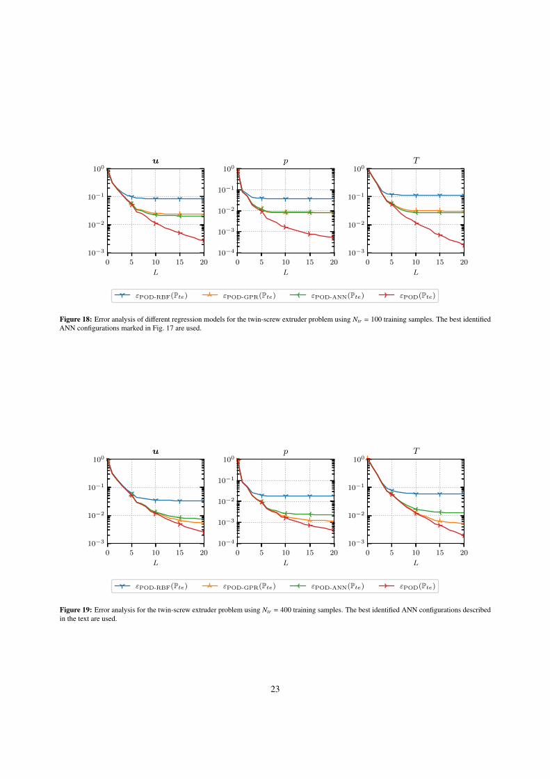
Fig. 18 depicts the best ANN configurations together with the other two regression models. Again, the tuned ANNdoes not outperform the GPR despite the computationally expensive hyperparameter tuning. Furthermore, the greaterflexibility of the ANN also requires making several decisions about the fixed and tuned hyperparameters, which usuallyboils down to empirical and tedious trial-and-error.Bear in mind, however, that our results suggest that these manual efforts can be avoided and an ANN can be trainedwith good success by following the described preprocessing steps, using the standardized error, and automatedhyperparameter search. Nevertheless, in all the investigated settings GPR is at least as good as ANN, despite it beingeasier to implement, train and interpret.For this problem, the performance of the RBF is significantly worse than in the other two problems. Even so, since itcan be implemented and trained in a fraction of time even compared to GPR, RBF regression can serve as a viableempirical upper-bound for the other models.To investigate the nature of errors, Fig. 20 illustrates the true temperature over several timesteps alongside the absoluteerror of the predicted solution computed using the POD-ANN. As expected, the errors are zero on the outer barrel,where the same Dirichlet boundary condition is prescribed to all high-fidelity solutions. The same cannot be observedon the adiabatic screws – particularly in regions where the warm melt sticks to the screw surface and is traced throughoutthe interior, the errors are the highest. Due to the right side being heated, the errors in the right barrel tend to be smallerthan in the left.At no point the temperature is off by more than 0.7. The ratio of the typical range of errors to the typical rangeof temperature, i.e., 1.4/40 happens to be close to the total standardized error for this sample at εPOD-ANN = 0.034,providing a good intuition behind the standardized error.Lastly, we illustrate the effect of increasing the number of training samples Ntr. This is an easy to implement yetcomputationally expensive approach to reducing the errors. Fig. 19 shows the errors over the number of bases L usingfour times as many training samples Ntr = 400 and the same validation and test sets as before.

22

0 5 10 15 20

L

10−3

10−2

10−1

100u

0 5 10 15 20

L

10−4

10−3

10−2

10−1

100p

0 5 10 15 20

L

10−3

10−2

10−1

100T

εPOD-RBF(Pte) εPOD-GPR(Pte) εPOD-ANN(Pte) εPOD(Pte)

Figure 18: Error analysis of different regression models for the twin-screw extruder problem using Ntr = 100 training samples. The best identifiedANN configurations marked in Fig. 17 are used.

0 5 10 15 20

L

10−3

10−2

10−1

100u

0 5 10 15 20

L

10−4

10−3

10−2

10−1

100p

0 5 10 15 20

L

10−3

10−2

10−1

100T

εPOD-RBF(Pte) εPOD-GPR(Pte) εPOD-ANN(Pte) εPOD(Pte)

Figure 19: Error analysis for the twin-screw extruder problem using Ntr = 400 training samples. The best identified ANN configurations describedin the text are used.

23

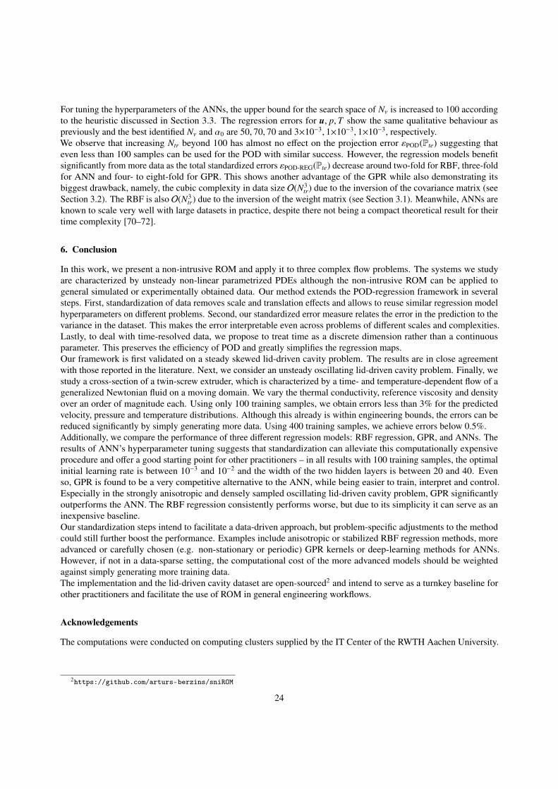
For tuning the hyperparameters of the ANNs, the upper bound for the search space of Nν is increased to 100 accordingto the heuristic discussed in Section 3.3. The regression errors for u, p,T show the same qualitative behaviour aspreviously and the best identified Nν and α0 are 50, 70, 70 and 3×10−3, 1×10−3, 1×10−3, respectively.We observe that increasing Ntr beyond 100 has almost no effect on the projection error εPOD(Pte) suggesting thateven less than 100 samples can be used for the POD with similar success. However, the regression models benefitsignificantly from more data as the total standardized errors εPOD-REG(Pte) decrease around two-fold for RBF, three-foldfor ANN and four- to eight-fold for GPR. This shows another advantage of the GPR while also demonstrating itsbiggest drawback, namely, the cubic complexity in data size O(N3

tr) due to the inversion of the covariance matrix (seeSection 3.2). The RBF is also O(N3

tr) due to the inversion of the weight matrix (see Section 3.1). Meanwhile, ANNs areknown to scale very well with large datasets in practice, despite there not being a compact theoretical result for theirtime complexity [70–72].

6. Conclusion

In this work, we present a non-intrusive ROM and apply it to three complex flow problems. The systems we studyare characterized by unsteady non-linear parametrized PDEs although the non-intrusive ROM can be applied togeneral simulated or experimentally obtained data. Our method extends the POD-regression framework in severalsteps. First, standardization of data removes scale and translation effects and allows to reuse similar regression modelhyperparameters on different problems. Second, our standardized error measure relates the error in the prediction to thevariance in the dataset. This makes the error interpretable even across problems of different scales and complexities.Lastly, to deal with time-resolved data, we propose to treat time as a discrete dimension rather than a continuousparameter. This preserves the efficiency of POD and greatly simplifies the regression maps.Our framework is first validated on a steady skewed lid-driven cavity problem. The results are in close agreementwith those reported in the literature. Next, we consider an unsteady oscillating lid-driven cavity problem. Finally, westudy a cross-section of a twin-screw extruder, which is characterized by a time- and temperature-dependent flow of ageneralized Newtonian fluid on a moving domain. We vary the thermal conductivity, reference viscosity and densityover an order of magnitude each. Using only 100 training samples, we obtain errors less than 3% for the predictedvelocity, pressure and temperature distributions. Although this already is within engineering bounds, the errors can bereduced significantly by simply generating more data. Using 400 training samples, we achieve errors below 0.5%.Additionally, we compare the performance of three different regression models: RBF regression, GPR, and ANNs. Theresults of ANN’s hyperparameter tuning suggests that standardization can alleviate this computationally expensiveprocedure and offer a good starting point for other practitioners – in all results with 100 training samples, the optimalinitial learning rate is between 10−3 and 10−2 and the width of the two hidden layers is between 20 and 40. Evenso, GPR is found to be a very competitive alternative to the ANN, while being easier to train, interpret and control.Especially in the strongly anisotropic and densely sampled oscillating lid-driven cavity problem, GPR significantlyoutperforms the ANN. The RBF regression consistently performs worse, but due to its simplicity it can serve as aninexpensive baseline.Our standardization steps intend to facilitate a data-driven approach, but problem-specific adjustments to the methodcould still further boost the performance. Examples include anisotropic or stabilized RBF regression methods, moreadvanced or carefully chosen (e.g. non-stationary or periodic) GPR kernels or deep-learning methods for ANNs.However, if not in a data-sparse setting, the computational cost of the more advanced models should be weightedagainst simply generating more training data.The implementation and the lid-driven cavity dataset are open-sourced2 and intend to serve as a turnkey baseline forother practitioners and facilitate the use of ROM in general engineering workflows.

Acknowledgements

The computations were conducted on computing clusters supplied by the IT Center of the RWTH Aachen University.

2https://github.com/arturs-berzins/sniROM

24

454 T 493 −0.7 T − T 0.7

Figure 20: The high-fidelity true solution T (µ = (1.01, 6.52×1012, 504) ∈ Pte) (left) and the error in prediction made by the best ANN (right) at timesteps t60, t65, t70, t75 and t80. Over all investigated timesteps the standardized error of the prediction is εPOD-ANN = 0.034.

25

References

[1] W. Chen, J. S. Hesthaven, B. Junqiang, Y. Qiu, Z. Yang, Y. Tihao, Greedy nonintrusive reduced order model for fluid dynamics, AIAA Journal56 (12) (2018) 4927–4943. doi:10.2514/1.j056161.

[2] A. Antoulas, N. Martins, E. Maten, K. Mohaghegh, R. Pulch, J. Rommes, M. Saadvandi, M. Striebel, Model Order Reduction: Methods,Concepts and Properties, 2015, pp. 159–265. doi:10.1007/978-3-662-46672-8_4.

[3] G. Rozza, H. Malik, N. Demo, M. Tezzele, M. Girfoglio, G. Stabile, A. Mola, Advances in reduced order methods for parametric industrialproblems in computational fluid dynamics, 2018.

[4] P. Benner, S. Gugercin, K. Willcox, A survey of projection-based model reduction methods for parametric dynamical systems., SIAM Review57 (4) (2015) 483–531.

[5] M. Eldred, D. Dunlavy, Formulations for surrogate-based optimization with data fit, multifidelity, and reduced-order models, in: 11thAIAA/ISSMO Multidisciplinary Analysis and Optimization Conference, American Institute of Aeronautics and Astronautics, 2006. doi:10.2514/6.2006-7117.

[6] M. H. Malik, Reduced Order Modeling for Smart Grids’ Simulation and Optimization, Ph.D. thesis, École centrale de Nantes ; Universitatpolitécnica de Catalunya (Feb. 2017).

[7] J. Yu, C. Yan, M. Guo, Non-intrusive reduced-order modeling for fluid problems: A brief review, Proceedings of the Institution of MechanicalEngineers, Part G: Journal of Aerospace Engineering 233 (16) (2019) 5896–5912. doi:10.1177/0954410019890721.

[8] J. Hesthaven, S. Ubbiali, Non-intrusive reduced order modeling of nonlinear problems using neural networks, Journal of Computational Physics363 (2018) 55–78. doi:10.1016/j.jcp.2018.02.037.

[9] M. Guo, J. S. Hesthaven, Reduced order modeling for nonlinear structural analysis using gaussian process regression, Computer Methods inApplied Mechanics and Engineering 341 (2018) 807–826. doi:10.1016/j.cma.2018.07.017.

[10] M. Guo, J. S. Hesthaven, Data-driven reduced order modeling for time-dependent problems, Computer Methods in Applied Mechanics andEngineering 345 (2019) 75–99. doi:10.1016/j.cma.2018.10.029.

[11] J. N. Kutz, S. L. Brunton, B. W. Brunton, J. L. Proctor, Dynamic Mode Decomposition: Data-Driven Modeling of Complex Systems,SIAM-Society for Industrial and Applied Mathematics, Philadelphia, PA, USA, 2016.

[12] J. S. Hesthaven, G. Rozza, B. Stamm, Certified Reduced Basis Methods for Parametrized Partial Differential Equations, 1st Edition, SpringerBriefs in Mathematics, Springer, 2015.

[13] M. Barrault, Y. Maday, N. C. Nguyen, A. T. Patera, An ‘empirical interpolation’ method: application to efficient reduced-basis discretization ofpartial differential equations, Comptes Rendus Mathematique 339 (9) (2004) 667–672. doi:10.1016/j.crma.2004.08.006.

[14] S. Chaturantabut, D. Sorensen, Discrete empirical interpolation for nonlinear model reduction, Vol. 32, 2010, pp. 4316 – 4321. doi:10.1109/CDC.2009.5400045.

[15] M. Rewienski, J. White, Model order reduction for nonlinear dynamical systems based on trajectory piecewise-linear approximations, LinearAlgebra and its Applications 415 (2-3) (2006) 426–454. doi:10.1016/j.laa.2003.11.034.

[16] V. Dolci, R. Arina, Proper orthogonal decomposition as surrogate model for aerodynamic optimization, International Journal of AerospaceEngineering 2016 (2016) 1–15. doi:10.1155/2016/8092824.

[17] T. Bui-Thanh, M. Damodaran, K. Willcox, Proper orthogonal decomposition extensions for parametric applications in transonic aerodynamics,2003.

[18] S. Walton, O. Hassan, K. W. Morgan, Reduced order modelling for unsteady fluid flow using proper orthogonal decomposition and radial basisfunctions, 2013.

[19] D. Xiao, F. Fang, C. Pain, G. Hu, Non-intrusive reduced-order modelling of the navier–stokes equations based on rbf interpolation, InternationalJournal for Numerical Methods in Fluids 79 (11) (2015) 580–595. doi:10.1002/fld.4066.

[20] E. Iuliano, D. Quagliarella, Proper orthogonal decomposition, surrogate modelling and evolutionary optimization in aerodynamic design,Computers & Fluids 84 (2013) 327–350. doi:10.1016/j.compfluid.2013.06.007.

[21] D. Xiao, F. Fang, C. Pain, I. Navon, A parameterized non-intrusive reduced order model and error analysis for general time-dependentnonlinear partial differential equations and its applications, Computer Methods in Applied Mechanics and Engineering 317 (2017) 868–889.doi:10.1016/j.cma.2016.12.033.

[22] R. Dupuis, J.-C. Jouhaud, P. Sagaut, Surrogate modeling of aerodynamic simulations for multiple operating conditions using machine learning,AIAA Journal 56 (9) (2018) 3622–3635. doi:10.2514/1.j056405.

[23] Q. Wang, J. S. Hesthaven, D. Ray, Non-intrusive reduced order modeling of unsteady flows using artificial neural networks with application toa combustion problem, Journal of Computational Physics 384 (2019) 289–307. doi:10.1016/j.jcp.2019.01.031.

[24] Z. Gao, Q. Liu, J. Hesthaven, B.-S. Wang, W. S. Don, X. Wen, Non-intrusive reduced order modeling of convection dominated flows usingartificial neural networks with application to rayleigh-taylor instability (06 2019).

[25] K. H. Park, S. O. Jun, S. M. Baek, M. H. Cho, K. J. Yee, D. H. Lee, Reduced-order model with an artificial neural network for aerostructuraldesign optimization, Journal of Aircraft 50 (4) (2013) 1106–1116. doi:10.2514/1.c032062.

[26] O. San, R. Maulik, M. Ahmed, An artificial neural network framework for reduced order modeling of transient flows, Communications inNonlinear Science and Numerical Simulation 77 (02 2018). doi:10.1016/j.cnsns.2019.04.025.

[27] D. Maier, On the use of model order reduction techniques for the elastohydrodynamic contact problem: Zugl.: Karlsruhe, KIT, Diss., 2015,Vol. 27 of Schriftenreihe des Instituts für Technische Mechanik, KIT Scientific Publishing, Karlsruhe, 2015.

[28] M. Girault, J. Launay, N. Allanic, P. Mousseau, R. Deterre, Development of a thermal reduced order model with explicit dependence on viscosityfor a generalized newtonian fluid, Journal of Non-Newtonian Fluid Mechanics 260 (2018) 26–39. doi:10.1016/j.jnnfm.2018.04.002.

[29] M. Ocana, D. Alonso, A. Velazquez, Reduced order model for a power-law fluid, Journal of Fluids Engineering 136 (2014) 071205.doi:10.1115/1.4026666.

[30] E. Muravleva, I. Oseledets, D. Koroteev, Application of machine learning to viscoplastic flow modeling, Physics of Fluids 30 (10) (2018)103102.

26

[31] C. Audouze, F. D. Vuyst, P. B. Nair, Nonintrusive reduced-order modeling of parametrized time-dependent partial differential equations,Numerical Methods for Partial Differential Equations 29 (5) (2013) 1587–1628. doi:10.1002/num.21768.

[32] B. Peherstorfer, K. Willcox, Data-driven operator inference for nonintrusive projection-based model reduction, Computer Methods in AppliedMechanics and Engineering 306 (2016) 196–215. doi:10.1016/j.cma.2016.03.025.

[33] J. Helmig, M. Behr, S. Elgeti, Boundary-conforming finite element methods for twin-screw extruders: Unsteady-temperature-dependent-non-newtonian simulations, Computers & Fluids 190 (2019) 322–336.

[34] E. Schmidt, Zur theorie der linearen und nichtlinearen integralgleichungen, Mathematische Annalen 63 (4) (1907) 433–476. doi:10.1007/bf01449770.

[35] C. Eckart, G. Young, The approximation of one matrix by another of lower rank, Psychometrika 1 (3) (1936) 211–218. doi:10.1007/bf02288367.

[36] L. Sirovich, Turbulence and the dynamics of coherent structures. i - coherent structures. ii - symmetries and transformations. iii - dynamics andscaling, Quarterly of Applied Mathematics - QUART APPL MATH 45 (10 1987). doi:10.1090/qam/910463.

[37] V. Y. Pan, Z. Q. Chen, The complexity of the matrix eigenproblem, in: Proceedings of the Thirty-First Annual ACM Symposium on Theory ofComputing, Association for Computing Machinery, New York, NY, USA, 1999, pp. 507–516. doi:10.1145/301250.301389.

[38] Y. LeCun, A theoretical framework for back-propagation, in: D. Touretzky, G. Hinton, T. Sejnowski (Eds.), Proceedings of the 1988Connectionist Models Summer School, CMU, Pittsburg, PA, Morgan Kaufmann, 1988, pp. 21–28.

[39] S. E. Ahmed, O. San, D. A. Bistrian, I. M. Navon, Sampling and resolution characteristics in reduced order models of shallow water equations:Intrusive vs nonintrusive, International Journal for Numerical Methods in Fluids (Feb. 2020). doi:10.1002/fld.4815.

[40] H. Chen, D. L. Reuss, V. Sick, On the use and interpretation of proper orthogonal decomposition of in-cylinder engine flows, MeasurementScience and Technology 23 (8) (2012) 085302. doi:10.1088/0957-0233/23/8/085302.

[41] P. Honeine, An eigenanalysis of data centering in machine learning, ArXiv abs/1407.2904 (2014).[42] Y. LeCun, L. Bottou, G. B. Orr, K.-R. Müller, Efficient backprop, in: Neural Networks: Tricks of the Trade, This Book is an Outgrowth of a

1996 NIPS Workshop, Springer-Verlag, Berlin, Heidelberg, 1998, p. 9–50.[43] A. Botchkarev, Performance metrics (error measures) in machine learning regression, forecasting and prognostics: Properties and typology,

ArXiv abs/1809.03006 (2018).[44] R. Schaback, A practical guide to radial basis functions, 2007.[45] P. Virtanen, R. Gommers, T. E. Oliphant, M. Haberland, T. Reddy, D. Cournapeau, E. Burovski, P. Peterson, W. Weckesser, J. Bright, S. J.

van der Walt, M. Brett, J. Wilson, K. Jarrod Millman, N. Mayorov, A. R. J. Nelson, E. Jones, R. Kern, E. Larson, C. Carey, I. Polat, Y. Feng,E. W. Moore, J. Vand erPlas, D. Laxalde, J. Perktold, R. Cimrman, I. Henriksen, E. A. Quintero, C. R. Harris, A. M. Archibald, A. H. Ribeiro,F. Pedregosa, P. van Mulbregt, S. . . Contributors, SciPy 1.0: Fundamental Algorithms for Scientific Computing in Python, Nature Methods 17(2020) 261–272.

[46] M. Kuß, Gaussian process models for robust regression, classification, and reinforcement learning, Ph.D. thesis, Technische Universität,Darmstadt (April 2006).URL http://tuprints.ulb.tu-darmstadt.de/674/

[47] C. E. Rasmussen, C. K. I. Williams, Gaussian Processes for Machine Learning (Adaptive Computation and Machine Learning), The MIT Press,2005.

[48] F. Pedregosa, G. Varoquaux, A. Gramfort, V. Michel, B. Thirion, O. Grisel, M. Blondel, P. Prettenhofer, R. Weiss, V. Dubourg, J. Vanderplas,A. Passos, D. Cournapeau, M. Brucher, M. Perrot, E. Duchesnay, Scikit-learn: Machine Learning in Python , Journal of Machine LearningResearch 12 (2011) 2825–2830.

[49] I. Goodfellow, Y. Bengio, A. Courville, Deep Learning, MIT Press, 2016, http://www.deeplearningbook.org.[50] O. I. Abiodun, A. Jantan, A. E. Omolara, K. V. Dada, N. A. Mohamed, H. Arshad, State-of-the-art in artificial neural network applications: A

survey, Heliyon 4 (11) (2018) e00938. doi:https://doi.org/10.1016/j.heliyon.2018.e00938.URL http://www.sciencedirect.com/science/article/pii/S2405844018332067

[51] S. Ruder, An overview of gradient descent optimization algorithms, ArXiv abs/1609.04747 (2016).[52] D. P. Kingma, J. Ba, Adam: A method for stochastic optimization, CoRR abs/1412.6980 (2014).[53] I. Sutskever, J. Martens, G. Dahl, G. Hinton, On the importance of initialization and momentum in deep learning, in: Proceedings of the 30th

International Conference on International Conference on Machine Learning - Volume 28, ICML13, JMLR.org, 2013, pp. III–1139–III–1147.[54] D. Choi, C. J. Shallue, Z. Nado, J. Lee, C. J. Maddison, G. E. Dahl, On empirical comparisons of optimizers for deep learning (2019).

URL http://arxiv.org/abs/1910.05446[55] R. Liaw, E. Liang, R. Nishihara, P. Moritz, J. E. Gonzalez, I. Stoica, Tune: A research platform for distributed model selection and training,

arXiv preprint arXiv:1807.05118 (2018).[56] A. Paszke, S. Gross, F. Massa, A. Lerer, J. Bradbury, G. Chanan, T. Killeen, Z. Lin, N. Gimelshein, L. Antiga, A. Desmaison, A. Kopf, E. Yang,

Z. DeVito, M. Raison, A. Tejani, S. Chilamkurthy, B. Steiner, L. Fang, J. Bai, S. Chintala, Pytorch: An imperative style, high-performancedeep learning library, in: Advances in Neural Information Processing Systems 32, Curran Associates, Inc., 2019, pp. 8024–8035.

[57] T. A. Osswald, N. Rudolph, Polymer Rheologyy: fundamentals and applications, Carl Hanser Verlag GmbH Co KG, 2014.[58] T. Tezduyar, M. Behr, J. Liou, A new strategy for finite element computations involving moving boundaries and interfaces-the deforming-

spatial-domain/space-time procedure: I. the concept and the preliminary numerical tests, Computer Methods in Applied Mechanics andEngineering 94 (1992) 339–351. doi:10.1016/0045-7825(92)90059-S.

[59] J. Donea, A. Huerta, Finite element methods for flow problems, John Wiley & Sons, 2003.[60] L. Pauli, M. Behr, On stabilized space-time fem for anisotropic meshes: Incompressible navier–stokes equations and applications to blood flow

in medical devices, International Journal for Numerical Methods in Fluids 85 (3) (2017) 189–209.[61] C. Gräßle, M. Hinze, J. Lang, S. Ullmann, POD model order reduction with space-adapted snapshots for incompressible flows, Advances in

Computational Mathematics 45 (5-6) (2019) 2401–2428. doi:10.1007/s10444-019-09716-7.[62] G. Stabile, G. Rozza, Finite volume POD-galerkin stabilised reduced order methods for the parametrised incompressible navier–stokes

equations, Computers & Fluids 173 (2018) 273–284. doi:10.1016/j.compfluid.2018.01.035.

27

[63] R. Deshmukh, J. J. McNamara, Z. Liang, J. Z. Kolter, A. Gogulapati, Model order reduction using sparse coding exemplified for the lid-drivencavity, Journal of Fluid Mechanics 808 (2016) 189–223. doi:10.1017/jfm.2016.616.

[64] M. Balajewicz, A new approach to model order reduction of the navier-stokes equations, 2012.[65] A. Dumon, C. Allery, A. Ammar, Simulation of heat and mass transport in a square lid-driven cavity with proper generalized decomposition

(PGD), Numerical Heat Transfer, Part B: Fundamentals 63 (1) (2013) 18–43. doi:10.1080/10407790.2012.724991.[66] C. E. Rasmussen, Evaluation of gaussian processes and other methods for non-linear regression, Ph.D. thesis, CAN, aAINQ28300 (1997).[67] G. Casciola, L. Montefusco, S. Morigi, The regularizing properties of anisotropic radial basis functions, Applied Mathematics and Computation

190 (2) (2007) 1050–1062. doi:10.1016/j.amc.2006.11.128.[68] R. Yondo, E. Andrés, E. Valero, A review on design of experiments and surrogate models in aircraft real-time and many-query aerodynamic

analyses, Progress in Aerospace Sciences 96 (2018) 23–61. doi:10.1016/j.paerosci.2017.11.003.[69] J. Hinz, J. Helmig, M. Möller, S. Elgeti, Boundary-conforming finite element methods for twin-screw extruders using spline-based parameteri-

zation techniques, Computer Methods in Applied Mechanics and Engineering 361 (2020) 112740.[70] R. Livni, S. Shalev-Shwartz, O. Shamir, On the computational efficiency of training neural networks, in: Proceedings of the 27th International

Conference on Neural Information Processing Systems - Volume 1, NIPS’14, MIT Press, Cambridge, MA, USA, 2014, p. 855–863.[71] D. Boob, S. S. Dey, G. Lan, Complexity of training relu neural network (2018). arXiv:1809.10787.[72] S. Goel, A. Klivans, Learning neural networks with two nonlinear layers in polynomial time (2017). arXiv:1709.06010.

28