Gravimetric determination of an intrusive complex under the

Geophys. J. Int. (2007) 171, 478–494 doi: 10.1111/j.1365-246X.2007.03539.xG

JIVol

cano

logy

,ge

othe

rmic

s,flui

dsan

dro

cks

Gravimetric determination of an intrusive complex under the Islandof Faial (Azores): some methodological improvements

Antonio G. Camacho,1 J. Carlos Nunes,2 Esther Ortiz,1 Zilda Franca2 and Ricardo Vieira1

1Instituto de Astronomıa y Geodesia (CSIC-UCM), Fac. CC. Matematicas. Ciudad Universitaria, Madrid 28040, Spain. E-mail: antonio [email protected] dos Acores – Departamento de Geociencias, Rua da Mae de Deus, Apartado 1422, 9501-801 Ponta Delgada, Azores, Portugal

Accepted 2007 June 26. Received 2007 June 26; in original form 2006 September 6

S U M M A R YWe present some improvements of a gravity inversion method to determine the geometry ofthe anomalous bodies for priori density contrasts. The 3-D method is based on an exploratoryprocess applied, not for the global model, but for the steps of a growth approach. The (positiveand/or negative) anomalous structure is described by successive aggregation of cells, whileits corresponding gravity field remains nearly proportional to the observed one. Moreover, asimple (e.g. linear) regional trend can be simultaneously adjusted. The corresponding programis applied to new gravity data on the volcanic island of Faial (Azores archipelago). The inver-sion approach shows a subsurface anomalous structure for the island, the main feature beingan elongated high-density body. The body is interpreted as a compact sheeted dyke swarm,emplaced along Faial-Pico Fracture Zone, a leaky transform structure that forms the currentboundary between Eurasian and African plates in the Azores area. The new results in this pa-per are (1) a Bouguer gravity anomaly map, (2) several improvements in the inversion process(robust process, optimal balance fitness/model magnitude), (3) a new gravimetric method forestimating the mean terrain density, (4) a 3-D model for subsurface mass anomalies in Faialand (5) some interpretative conclusions about a main intrusive complex detected under theisland as a wall-like structure extending from a depth of 0.5 to 6 km b.s.l., with a N100◦E trendand corresponding to an early fissural volcanic episode controlled by the regional tectonics.

Key words: Faial (Azores), gravity anomalies, inverse problem, volcanic structure.

1 I N T RO D U C T I O N

According to Walker (1999), rift zones and underlying dyke swarmsoccur in most volcanoes and contain the paths taken by magmasmoving through the crust. Most of these intrusive complexes arepositioned and oriented by tectonic structures or may be propagatedlaterally from volcanic centres along rift zones, following neutralbuoyancy levels.

Sheeted dyke complexes are detected in oceanic-spreading set-tings and in the core regions of major volcanoes. They may containthousands of very narrow dykes or other sheet-like intrusions asswarms that increase abruptly in intensity at their edges. Dyke com-plexes are perceived to grow incrementally by the addition of dykesalong their margins, and are self-sustaining (Walker 1999). Addi-tionally, incoming magma batches are guided by the many planesof weakness in the complex. Closer to the surface, swarms of sheetintrusions (dykes and sills) represent conduits for magma transportfrom the reservoirs to the surface or to shallow intrusions, the set-ting of this latter type of intrusions being well documented in activevolcanoes, such as Kilauea or Piton de la Fournaise (Malengreau

et al. 1999). Walker (1999) also suggests that intrusion of dykesmay cause bending or initiation of a rift zone.

Large swarms of intrusive bodies can be gravimetrically deter-mined. Accordingly to Rymer & Brown (1986), positive anoma-lies characterize mainly basaltic volcanoes, and are caused by arelatively dense intrusive complex/magma body, which contrastswith its surroundings either because that intrusive body is moremafic than average or, more likely, because near surface, previ-ously erupted materials are uncompacted, with a higher degree ofvesiculation. Walker (1992) for Hawaiian volcanoes considers anintrusive complex with density 2800 kg m–3 juxtaposed againsthighly vesicular lava flows having a much lower density of about2000 kg m–3. Ryan (1987 in Malengreau et al. 1999) proposedthat complexes of hypovolcanic intrusions and cumulates developupwards during growth of a volcano. As a result, the centre of amature oceanic shield volcano is expected to be characterized by acolumn-like body of high-density rock that can be detected throughgravimetric observation and modelled by some inversion approach.Apart from the general ambiguity problem of the gravity inversion,some problems arise from the accessibility and sharp topographic

478 C© 2007 The Authors

Journal compilation C© 2007 RAS

Dow

nloaded from https://academ

ic.oup.com/gji/article/171/1/478/2126298 by guest on 28 June 2022

Gravimetric inversion for Faial (Azores) 479

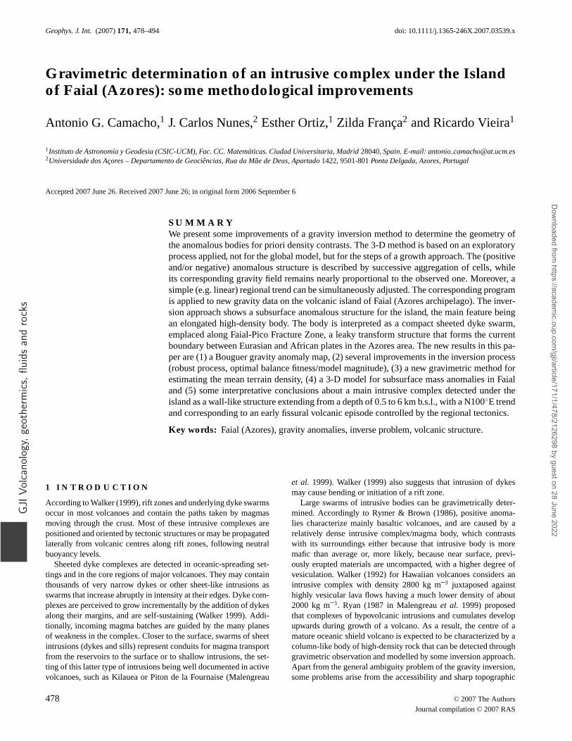
Figure 1. General geotectonic framework of Azores archipelago, at the triple junction of Eurasian, North American and African plates. Location of Faial Islandis highlighted. M.A.R.: Mid-Atlantic Ridge; FPFZ: Faial-Pico Fracture Zone; EAFZ: East Azores Fracture Zone. Simplified from: Montesinos et al. (2003).

effects in volcanic areas mainly formed by very high bulk densitymaterial.

The Azores archipelago is located in the North Atlantic Ocean,between latitudes 37◦ and 40◦N and longitudes 25◦ and 31◦W, atthe triple junction of Eurasian, North American and African litho-spheric plates (Fig. 1). It consists of nine islands and several isletsof volcanic nature that emerge from an anomalously shallow andrough topographic zone, the so-called ‘Azores Plateau’ (Needham& Francheteau 1974), which is roughly triangular-shaped and isdefined by the 2000 bathymetric contour line. This area broadlycoincides with the Azores ‘microplate’or ‘block’, bordered by theMid-Atlantic Ridge (M.A.R.), the Terceira Rift and the East AzoresFracture Zone (EAFZ, Fig. 1), and it is characterized by recent andactive volcanoes and high seismicity (Searle 1980; Luis et al. 1994;Lourenco et al. 1998; Luis et al. 1998). The islands are alignedalong major tectonic lineaments with a general WNW–ESE trend,with the M.A.R. placed between Faial and Flores islands (Fig. 1).

Faial Island is located about 120 km east of the M.A.R., on theseismically active Faial-Pico Fracture Zone (FPFZ, Fig. 1). Thisstructure is a 350 km long leaky transform that extends from theM.A.R. with an ESE trend, and is considered by some (e.g. Luiset al. 1994) as the third arm of the Azores triple junction and, there-fore, the present boundary between the Eurasian and African plates.

The following sections present a process for determining a well-defined intrusive complex beneath the volcanic island of Faial. First,we present information about the geology and tectonics of the island.Secondly, we describe the gravity survey and the resulting Bougueranomaly map. Then, we present the inversion method applied to thegravity anomaly. This method is based on an exploratory solutionof the general non-linear three-dimensional (3-D) problem usinginexact data. A simulation test is added for better understanding ofthe process. The application of the method to the anomaly of Faialproduces a 3-D model of anomalous masses. This model shows thepresence of an interesting high-density body located on the central-eastern part of Faial Island. The final sections discuss the resulting

density structure model and its implications for an intrusive complexbeneath the island.

2 G E O L O G Y A N D V O L C A N O L O G Y O FFA I A L I S L A N D

The geology of Faial island (21 km length and 173 km2) is in generalterms dominated by a central volcano with caldera (‘Caldeira Vol-cano’) and by a western peninsula (‘Capelo’ Peninsula) built by 20scoria cones and related basaltic lava flows (Fig. 2). Near the townof Horta, about one dozen scoria cones are emplaced along NW–SEtrending fractures and are all covered with pumice deposits from thecentral volcano caldera. The eastern part of the island is character-ized by the Pedro Miguel Graben, which has a N115◦E average trendand width of about 7 km. In this eastern area, near Espalamaca, arethe oldest rocks of Faial, dated 730 000 yr before present (BP) byFeraud et al. (1980). They are related to an old shield volcano—the‘Ribeirinha’ Volcano—centred east of ‘Caldeira’ and are coveredby its younger trachytic products (Figs 2 and 3).

The ‘Caldeira Volcano’ has a maximum altitude of 1043 m, av-erage base diameter of 14 km, area of 133 km2, volume of about48 km3 (Nunes et al. 2004) and is built mostly by lava flows ofbasaltic to benmoreitic composition. Its late eruptive history duringthe past 10 000 yr (Madeira 1998; Pacheco 2001) is characterized byexplosive trachytic eruptions, accompanied by voluminous pumicefall deposits, ignimbrites and lahars (Serralheiro et al. 1989). Dur-ing those late explosive eruptions, a caldera 2 km wide and about400 m deep was formed (Fig. 2).

Basaltic volcanism dominates on the Capelo peninsula, withabout twenty Holocene eruptions, the last being the 1957–1958Capelinhos surtseyan eruption, located on its westernmost end. Thateruption added 1.5 km2 of new land to the island, and gave rise to1.5 m maximum subsidence during the May 1958 seismic crisis(Machado 1958; Tazieff 1959; Machado et al. 1962), as well as theopening of several tension cracks.

C© 2007 The Authors, GJI, 171, 478–494


Dow



480 A. G. Camacho et al.

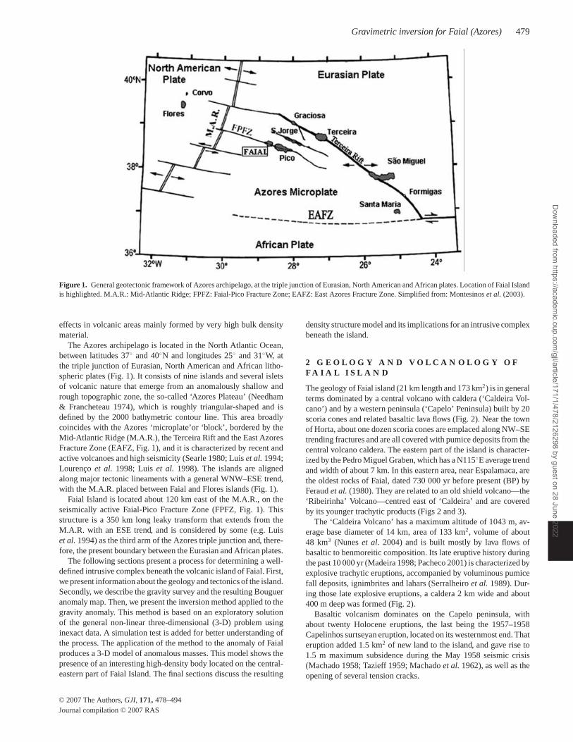
Figure 2. Main volcanic and tectonic features of Faial island: (1) caldera rim; (2) Pedro Miguel Graben faults; (3) main volcanotectonic lineaments, includingscoria cone vents (∗); (4) Castelo Branco (CB) and Altar (at Caldeira) trachytic domes; in grey- tuff cones of Monte da Guia (M), Costado da Nau (N) andCapelinhos (C). Modified after Serralheiro et al. (1989) and Madeira (1998).

As mentioned, the ‘Pedro Miguel Graben’ is the most prominentfeature in the eastern part of Faial Island: its fault scarps face SWand NE, with maximum height of about 170 m. The lowest block ofthat structure is located near Pedro Miguel village (Fig. 2). Close tothe central volcano summit the graben is mostly covered/filled bypumice and other Holocene pyroclastic deposits, but it can be tracedagain west of the ‘Caldeira’, namely at Ribeira Funda fault, even lessclear on the topography (Fig. 3). Pedro Miguel fault scarps starteddeveloping during the last 73 000 (or 40 000) yr, then channelledthe pyroclastic flow deposits (e.g. lahars and ignimbrites) extrudedduring the ‘Caldeira’ episodes (Madeira 1998). According to Tazieff(1959), Pedro Miguel Graben is merely a pure tectonic structure thatinfluenced the volcanism on Faial Island. According to MacDonald(1972) the graben is the result (1) of the removal of magma froman underlying magma chamber, (2) the result of stretching of thesurface of the volcano or (3) the result of stretching of the entireunderlying crust, due to the spreading associated with the AtlanticOcean.

3 G R AV I T Y DATA A N D A N O M A LY

In 2000, a gravity survey was conducted on the island of Faial on253 stations (Fig. 4) with a mean spacing of 800 m. A total of 274observations were carried out using a LaCoste&Romberg gravime-ter (G665) with electronic output. Observations were corrected for

tidal variations. Then we determined an instrument drift by fittingtraverses with a mean residual value about 0.02 × 10−5 m s−2 forrepeated stations. Gravity values were referenced to the absolutegravity value g = 980 129 217 (±0.007) × 10−5 m s−2 determinedin 1997 with the GILAg-5 of the Finnish Geodetic Institute (Bastoset al. 1999) on the seismic pillar of the Meteorological Observatoryof Horta (Faial) (main gravity base station for the island, Coelho1968).

A contemporaneous GPS differential survey was applied to de-termine station coordinates, mainly elevations. Observations werecarried out with an Ashtech Z-Surveyor equipment and, for the finalfit, we employed geodetic values for eight bench-marks as a refer-ence network on the island. The estimated accuracy of the resultingelevation values is about 0.05 m.

As part of gravity processing, we used a digital terrain model(DTM) for the island formed by 69 474 points arranged on a gridwith 50 m resolution. In addition, we consider the bathymetry forthe neighbouring areas (within a distance of 80 km) coming fromthe data files of global topography in SRTM30 format distributed bythe USGS EROS data centre, and corresponding to a grid with 30s resolution (http://topex.ucsd.edu/WWW html/srtm30 plus.html;Smith & Sandwell 1997). This terrain model was used for the relieffeatures in Fig. 3. Taking into account the rough resolution of theDTM, some very local residual effects can be suspected after theterrain correction.

C© 2007 The Authors, GJI, 171, 478–494


Dow




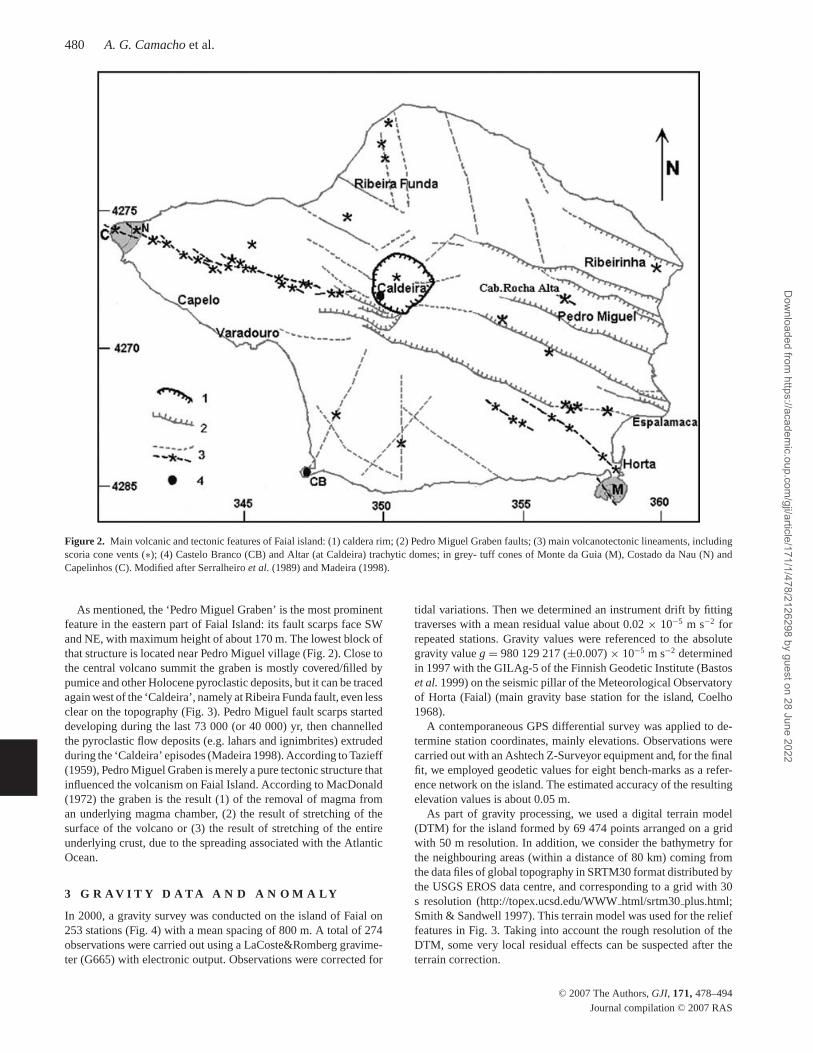
Figure 3. DEM for Faial Island (up) and superimposed main volcanotectonic structures of the island (down). (1) Capelinhos Volcano, (2) faults and (3) mainvolcanotectonic lineaments. General volcanostratigraphy: H: Historical eruptions (with year of occurrence), C: Capelo Volcanic Complex, V: Caldeira Volcano,B: Horta Basaltic Zone, G: Ribeirinha Volcano and Pedro Miguel Graben (adapted from Nunes, 2004).

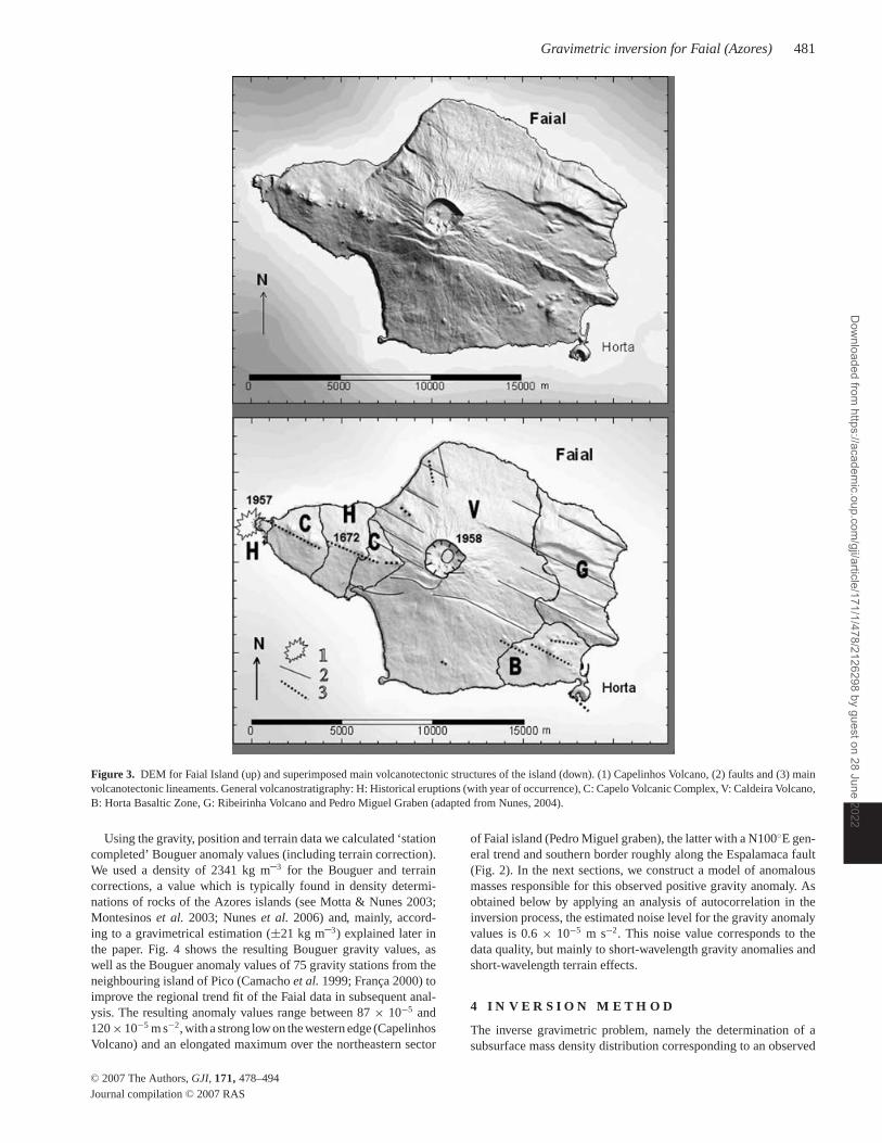
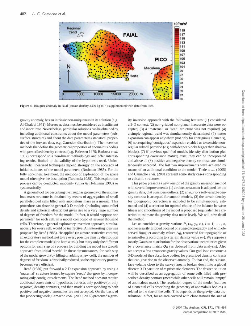
Using the gravity, position and terrain data we calculated ‘stationcompleted’ Bouguer anomaly values (including terrain correction).We used a density of 2341 kg m–3 for the Bouguer and terraincorrections, a value which is typically found in density determi-nations of rocks of the Azores islands (see Motta & Nunes 2003;Montesinos et al. 2003; Nunes et al. 2006) and, mainly, accord-ing to a gravimetrical estimation (±21 kg m–3) explained later inthe paper. Fig. 4 shows the resulting Bouguer gravity values, aswell as the Bouguer anomaly values of 75 gravity stations from theneighbouring island of Pico (Camacho et al. 1999; Franca 2000) toimprove the regional trend fit of the Faial data in subsequent anal-ysis. The resulting anomaly values range between 87 × 10−5 and120 × 10−5 m s−2, with a strong low on the western edge (CapelinhosVolcano) and an elongated maximum over the northeastern sector

of Faial island (Pedro Miguel graben), the latter with a N100◦E gen-eral trend and southern border roughly along the Espalamaca fault(Fig. 2). In the next sections, we construct a model of anomalousmasses responsible for this observed positive gravity anomaly. Asobtained below by applying an analysis of autocorrelation in theinversion process, the estimated noise level for the gravity anomalyvalues is 0.6 × 10−5 m s−2. This noise value corresponds to thedata quality, but mainly to short-wavelength gravity anomalies andshort-wavelength terrain effects.

4 I N V E R S I O N M E T H O D

The inverse gravimetric problem, namely the determination of asubsurface mass density distribution corresponding to an observed

C© 2007 The Authors, GJI, 171, 478–494


Dow




Figure 4. Bouguer anomaly in Faial (terrain density 2390 kg m–3) supplemented with data from Pico.

gravity anomaly, has an intrinsic non-uniqueness in its solution (e.g.Al-Chalabi 1971). Moreover, data must be considered as insufficientand inaccurate. Nevertheless, particular solutions can be obtained byincluding additional constraints about the model parameters (sub-surface structure) and about the data parameters (statistical proper-ties of the inexact data, e.g. Gaussian distribution). The inversionmethods that define the geometrical properties of anomalous bodieswith prescribed density contrast (e.g. Pedersen 1979; Barbosa et al.1997) correspond to a non-linear methodology and offer interest-ing results, limited to the validity of the hypothesis used. Unfor-tunately, linearized techniques depend strongly on the accuracy ofinitial estimates of the model parameters (Rothman 1985). For thefully non-linear treatment, the methods of exploration of the spacemodel often give the best option (Tarantola 1988). This explorationprocess can be conducted randomly (Silva & Hohmann 1983) orsystematically.

A general tool for describing the irregular geometry of the anoma-lous mass structure is obtained by means of aggregation of smallparallelepiped cells filled with anomalous mass as a mosaic. Thisprocedure can describe general 3-D models (including some reliefdetails and spherical effects) but gives rise to a very large numberof degrees of freedom for the model. In fact, it would suppose oneparameter for each cell, in a model composed of several thousandcells. Therefore, a general exploratory inversion approach, simulta-neously for every cell, would be ineffective. An interesting idea wasproposed by Rene (1986). He applied (in a more restrictive context)an exploratory method, not to try every possible density distributionfor the complete model (too hard a task), but to try only the differentoptions for each step of a process for building the model in a growthapproach from initial ‘seeds’. In these circumstances, for each stepof the model growth (by filling or adding a new cell), the number ofdegrees of freedom is drastically reduced, so the exploratory processbecomes very efficient.

Rene (1986) put forward a 2-D expansion approach by using a‘maternal’ structure formed by square ‘seeds’ that grow by incorpo-rating only contiguous elements. The Rene method does not requireadditional constraints or hypotheses but uses only positive (or onlynegative) density contrasts, and then models corresponding to bothpositive and negative anomalies are not accepted. On the basis ofthis pioneering work, Camacho et al. (2000, 2002) presented a grav-

ity inversion approach with the following features: (1) considereda 3-D context, (2) non-gridded non-planar inaccurate data were ac-cepted, (3) a ‘maternal’ or ‘seed’ structure was not required, (4)a simple regional trend was simultaneously determined, (5) matterexpansion can appear anywhere (not only for contiguous elements),(6) not requiring ‘contiguous’ expansion enabled us to consider non-regular subsoil partition (e.g. with deeper blocks bigger than shallowblocks), (7) if previous qualified models (density distribution pluscorresponding covariance matrix) exist, they can be incorporatedand above all (8) positive and negative density contrasts are simul-taneously accepted. The last two improvements were achieved bymeans of an additional condition to the model. Tiede et al. (2005)and Camacho et al. (2001) present some study cases correspondingto volcanic structures.

This paper presents a new version of the gravity inversion methodwith several improvements: (1) a robust treatment is adopted for thegravity data, that considers outliers, (2) an a priori self-variable den-sity contrast is accepted for smooth models, (3) the terrain densityfor topographic correction is included to be simultaneously esti-mated and (4) a criterion for optimal choice of the balance betweenfitness and smoothness of the model is proposed (equivalent to a cri-terion to estimate the gravity data noise level). We will now detailthe method.

Let us consider n gravity stations Pi (xi, yi, zi), i = 1, . . . , n,not necessarily gridded, located on rugged topography and with ob-served Bouguer anomaly values �gi (corrected for topographic orterrain effects according to a terrain density value ρT). We suppose amostly Gaussian distribution for the observation uncertainties givenby a covariance matrix QD (as deduced from data analysis). Alsowe accept a few erroneous gravity values. Our goal is to construct a3-D model of the subsurface bodies, for prescribed density contraststhat can give rise to the observed anomaly. To that end, the subsur-face volume close to the survey area is broken down into a globaldiscrete 3-D partition of m prismatic elements. The desired solutionwill be described as an aggregation of some cells filled with pre-scribed density contrast (meanwhile other cells will remain ‘empty’of anomalous mass). The resolution degree of the model (numberof elemental cells describing the geometry of anomalous bodies) isrelated to the size of the cells. This depends on the gravity data dis-tribution. In fact, for an area covered with close stations the size of

C© 2007 The Authors, GJI, 171, 478–494


Dow




the cells could be smaller than for an area with far stations. Finally,the number of cells and the resolution of the model are limited byour computing capacity.

As usual for these non-linear methods, the few values of densitycontrasts that are going to be used to constitute the anomalous model(by filling some cells) are previously prescribed. For the jth cell wedecide an a priori positive contrast �ρ+

j (if excess of mass is finallyfitted there) and an a priori negative contrast �ρ−

j (if defect of massis finally fitted). In Section 5.1, we further detail how the startingvalues for �ρ+

j and �ρ−j have been chosen. The possibility of non-

anomalous mass (‘empty’ cell) is the third option.The gravity attraction, Aij, at the ith station Pi(xi, yi, zi), due to

the jth prism, for unit density, is given by Pick et al. (1973):

Ai j = −G{[

(x ln(y + (x2 + y2 + z2)1/2)

+ y ln(x + (x2 + y2 + z2)1/2)

+ z arctg(z(x2 + y2 + z2)1/2x−1 y−1))u j

2−xi

u j1−xi

]vj2 −yi

vj1 −yi

}wj2 −zi

wj1 −zi

,

(1)

where G is the gravitational constant, the edges of the jth prism areparallel to the reference axes, and the limiting coordinates for itsvolume are: uj

1, uj2 for the x coordinates, vj

1, vj2 for the y coordinates

and wj1, wj

2 for z. A 3-D mosaic with prisms can approximate the ir-regular volume to study. Matrix A, with components Aij is the designmatrix of the physical configuration of the problem and contains theeffect of the rugged terrain, the station distribution, the partition ofsubsurface volume, etc. Now the resulting model must reproducethe observed anomaly (except the observation noise):

�gi =∑j∈J+

Ai j�ρ+j +

∑j∈J−

Ai j�ρ−j

+δgreg + δgtop + vi , i = 1, . . . , n, (2)

where J+, J− are the sets of indexes corresponding to the cellsfilled with positive and negative density contrasts, δgreg representsa component corresponding to a regional smooth trend, δg top is anadditional term for revision of the topographic correction and vi

is a residual value which represents the local noise. It is notablethat we include the regional trend and the topographic correction(or, better, a corrective term to the topographic term used in thegravity reduction) as a part of the inversion approach instead of atreatment before inversion. For simplicity, we are going to adopt alinear expression for the regional trend component δgreg:

δgreg = p0 + px (xi − xM ) + py(yi − yM ), i = 1, . . . , n, (3)

where xM , yM are the planar (UTM, for instance) coordinates ofan arbitrary central point for the survey, and p0, px, py are threeunknown values which adjust a trend. A 1-degree polynomial sur-face is chosen because it simplifies the subsequent formulation andusually it is able to properly fit the very long wavelength compo-nent of the data. However, higher degree polynomial surfaces canbe implemented in a similar way. Below (Section 5.5) we give someadditional comments about the regional trend. On the other hand,the topographic correction term will have the following expression:

δgtop = δρT Ci , (4)

where δρT will be the unknown terrain density (or, better, a cor-rection of a terrain density previously adopted in the gravity reduc-tion) and Ci will be a coefficient depending on the relief geometryaround point Pi(xi, yi, zi). Below, we give more details about these

two corrective terms. So on, J+, J−, p0, px, py and δρT are the mainunknowns to be determined in this inversion process.

Previous information about the model structure, if known, canbe optionally incorporated. To that end, we express this informationas initial values ρo

j , j = 1, . . . , m, for the prism densities and acorresponding covariance matrix QM corresponding to the previousmodel confidence (Tarantola 1988) (bold character will be usedfor matrices and column vectors). For a problem without previousinformation about the model structure, we can adopt ρo

j = 0, j = 1,. . ., m, and take a model covariance matrix QM given by a diagonalnormalizing matrix of non-null elements that are the same as thediagonal elements of AT QD

−1A. (The elements of this matrix canbe used also to limit the whole subsurface volume in study, boundingthe accepted model uncertainty). The gravity values calculated forthis initial density structure at points Pi, i = 1, . . . , n, are:

�g0i =

m∑j=1

Ai j ρ0j (5)

to be removed from the observed anomaly.If only a minimization criterion for the residuals v is used, the ac-

ceptance of positive and negative values for the prescribed densitycontrasts and the inclusion of the trend unknowns give an inherentnon-unique solution. To solve this, an additional condition of mini-mization of the model variation can be adopted. Thus, the solutionis obtained by a mixed condition formed by the gravity l2-fitnessand the whole anomalous mass quantity, using a parameter λ for thesuitable balance:

vT Q−1D v + λ mT Q−1

M m = min, (6)

where v = (v11 , . . . , vn)T (T for transpose) are the gravity residualsfor the N stations, m = (�ρ11 , . . . , �ρm)T is the anomalous densityfor the m cells of the subsurface volume partition �ρ+

j or �ρ−j for

the filled cells and zero for those not filled), λ is a positive factor,empirically fixed, for balance between model fitness and anomalousmodel magnitude (and complexity). QD is the covariance matrix(usually diagonal matrix) corresponding to the estimated (Gaussian)inaccuracies of the gravity data, and QM is the covariance matrix cor-responding to the supposed determinability of the model parametersm. The first addend of the minimization functional (6) correspondsto the fit residuals weighted with the data quality matrix. The secondaddend is a weighted addition of the model densities. Nevertheless,taking into account that the covariance matrix QM contains the in-verse values of the squared prism volumes as factor, this secondaddend is connected with the anomalous mass or magnitude of themodel.

The λ parameter governs the application of the minimization con-ditions regarding the balance between total anomalous mass andresidual values. For low λ values a good fit is obtained, but themass of the anomalous model may increase excessively and ficti-tious structures may appear, mainly trying to fit the data noise. Forhigh λ values the adjusted model can be too slight, with too littlemass, and a poor gravity fit is obtained. Below we propose a prac-tical criterion for choosing optimal λ values and then determiningthe noise level in the gravity data.

The inversion process seeks to determine an anomalous modelgeometrically, described as an aggregation of cells filled with the apriori density contrasts (positive and negative), so that it verifies theminimization condition (6). As previously pointed out, we addressthis non-linear problem with a process that explores the large num-ber of possible models looking for the best one. A pure explorativemethod would consider every (!) possible model, trying their fit to

C© 2007 The Authors, GJI, 171, 478–494


Dow




the minimization conditions. The highly tedious task of global ex-ploration can be avoided by using a ‘growth’ process or expansionapproach to construct the anomalous bodies. The bodies are formedin a nearly homothetic growth by adding cells, from former ‘skele-tal’ structures, also adjusted, until they attain a suitable size. Then,the exploration of all the model’s possibilities is substituted by ex-ploration of the several possibilities of growth (cell by cell) for eachstep of the anomalous bodies expansion. This is a more reasonablegoal. Thus, the prismatic cells are systematically tested, step by step,with each prescribed density, and then the best options are adoptedand added to the growth approach for the anomalous bodies set-up.The minimization fit conditions are applied for each growth step,now including a scale factor f which relates the immature model tothe global conditions concerning gravity fit and model magnitude.Further details are given below.

For an arbitrary (k + 1)th step, k prisms have been previouslyfilled with the positive or negative fixed contrast values (or changedfrom some initial values) and the modelled gravity values will be:

�gci = � g0

i +∑J+

k

Ai j �ρ+j +

∑J−

k

Ai j �ρ−j , (7)

where J +k , J −

k are the index sets corresponding to the previouslymodified prisms with densities ρo

j + �ρ j . Now, we look for one newprism to modify throughout the m–k unchanged prisms. For eachjth unchanged prism, j /∈ J +

k , J −k , the following equation system can

be considered:

� gi − (� gc

i + Ai j �ρ j

)f − [p0 + px (xi − xM ) + py(yi − yM )]

− δρT Ci = vi i = 1, . . . , n, (8)

where �ρ j can take values �ρ+j and �ρ−

j and f ≥ 1 is an unknownscale factor for fitting the ‘actual’ model anomalies (�gc

i + Aij �ρ j )to the observed ones, �gi. The positive and the negative prescribedvalues are successively tested for the additional density contrast �ρ j

looking for the minimization condition (6).Next, the unknown parameters f , p0, px, py and δρT are adjusted

for a mix minimization criterion corresponding to this (k + 1)thstep:

vT Q−1D v + λ f 2 mT Q−1

M m = min, (9)

where the vector m of solutions now includes the values for thepreviously filled cells and the value �ρ j that is being tested:

m = (ml )T with : ml = �ρ j , ml = �ρ+l if l ∈ J +

k ,

ml = �ρ−l if l ∈ J −

k , otherwise ml = 0.To describe the solution, now we introduce the n-vectors r, g, u, x,y and z defined by the following ith components:

(x)i = xi − xM , (y)i = yi − yM , (z)i = Ci , (u)i = 1,

(r )i = � gci + Ai j �ρ j , (g )i = � gi

and then we introduce the following notation

smm = mT Q−1M m and sab = aT Q−1

D b, (10)

where the subscripts a and b and vectors a, b correspond to pairs ofsubscripts r, g, u, x, y and z referring to the former vectors r, g, u,x, y and z. With this notation, the normal equations correspondingto the system eqs (8) and (9) can be written as:

f srr + p0sru + px sr x + pysry + pzsrz − srg + λ f smm = 0

p0suu + f sru + px sxu + pysyu + pzszu − sgu = 0

p0sux + f sr x + px sxx + pysyx + pzszx − sgx = 0 (11)

p0suy + f sry + px sxy + pysyy + pzszy − sgy = 0

p0suz + f srz + px sxz + pysyz + pzszz − sgz = 0.

The solutions of the equation system (11) can be calculated forthe adopted prism and �ρ j as:

f = (srg − p0 sru − px sr x − py sry −pzsrz)/(srr +λ smm),

p0 = (Fug − px Fux − py Fuy −pz Fuz)/ Fuu,

px = (Gxg − py Gxy −pz Gxz)/ Gxx , (12)

py = (Myg −pz Myz)/ Myy,

pz = Nzg / Nzz,

where the following abbreviation coefficients

Fab = sab(srr + λsmm) − srasrb

Gab = Fab Fuu − Fua Fub (13)

Mab = GabGxx − Gxa Gxb

Nab = Mab Myy − Mya Myb

have been introduced.Once the former linear equations have been solved, we can cal-

culate the corresponding residual values v i in terms of the selected�ρ j. Then, we take the global misfit value e2

j defined by:

e2j = vT Q−1

D v + λ f 2 mT Q−1M m (14)

as the parameter for the suitability of jth prism and the densitypossibility (positive �ρ+

j or negative �ρ−j ) adopted. So, in this

(k + 1)th step, the method tests each of the unchanged prisms andboth (negative and positive) density contrast possibilities. Then, thejth prism and selected density (positive and negative) which producea minimum value of e2

j , which we will call E(k + 1), are definitivelyselected to increase the model, adding their effect to the model values�gi

c.This process is successively repeated. For the successive steps, the

scale value f decreases and the additional parameters p0, px, py andδT reach nearly stable values. The process stops when f approaches1, resulting in the modelled structure for anomalous density, a finalregional trend and a value (or a corrective one) for the terrain density.

Finally, the solution appears as a 3-D distribution of prismaticcells that have been assigned some of the prescribed contrast den-sities. Moreover, a regional trend and a terrain density are also ob-tained that supplements this anomalous mass distribution. Follow-ing this broad outline of the method, we now present now severalcomments and additional developments.

5 A D D I T I O N A L C O M M E N T S O N T H EI N V E R S I O N P RO C E S S

To simplify the foregoing description of the inversion method, wehave moved certain comments and additional explanations to thissection.

C© 2007 The Authors, GJI, 171, 478–494


Dow




5.1 A priori anomalous density contrasts: smoothingof the 3-D model boundaries

The present inversion method requires, as usual for many non-linearmethods, a suitable choice of the a priori density contrasts (positiveand negative, in our case). An excessively high density contrast willfit the main anomaly component but will produce a rather ‘skeleton’model, perhaps unable to represent small anomaly components. Anexcessively low density contrast will fit light structures, but wouldproduce a rather ‘inflated’ model, perhaps unable (taking into ac-count the volume limitations) to fit the main components, givingrise to fictitious peripheral bodies. To solve this issue, particularlyin the case when knowledge of the true local density contrasts isnot available, we adopt an alternative theoretical approach. Insteadof invariable local density contrasts along the whole model forma-tion process, we adopt contrasts that can vary. Starting from fixedmaximum values (let us name R+

j positive and R−j negative for each

jth cell), the prescribed density contrasts evolve along the growthprocess according to a simple law. By means of empirical tests, wehave selected for each growth step the density contrasts, �ρ+

j and�ρ−

j , positive and negative, given by:

�ρ+j = R+

j e−τ f , �ρ−j = R−

j e−τ f , (15)

where the scale factor, f ≥ 1, corresponding to the step of the fitprocess is used as characteristic parameter to describe the growthinstant and τ is a fixed factor corresponding to the desired variabil-ity of the density values. A high τ value will produce an anomalousmodel with contrast values mostly close to the maximum values(and then homogeneous with a sharp geometry). A low τ value willproduce a model with more variable contrasts, decreasing outwards(and then with a more diluted geometry). In this form, the high-density contrasts (close to the maximum values R+

j and R−j ) will

be employed to suitably fit the main anomaly components, whilesmaller density contrast suitably fit the smaller and local anoma-lies. The resulting anomalous model is more versatile (and perhapssomewhat more diluted).

Let us observe that the process indicated here pursues an inverseobjective to the one sought by the so-called ‘flatness’ constraint usedin the linear problem inversion. Indeed, when the densities of thegeometric elements (linear direct problem) are used as unknowns,the solution is too diluted or smooth, barely permitting specificbodies to be defined. Therefore, it becomes necessary to includea flatness condition based on the first derivatives of the densitydistribution, and that tends to favour better defined models (morehomogeneous on the inside and with sharper density changes on theoutside) (see Boulanger & Chouteau 2001; Bertete-Aguirre et al.2002). In contrast, the arbitrary smoothness condition imposed hereoptionally permits the opposite effect: to slightly dilute the edges ofthe bodies.

5.2 Optimum balance between observed data fit andcomplexity of the model

The parameter λ governs the method minimization conditions re-garding the balance between the model complexity (roughness, to-tal anomalous mass) and observation data fit (mean residual). Forsmall values of λ (and supposing a fine enough partition of the sub-soil volume) a very complete data fit is obtained, and even part ofthe observational noise is fitted. However, in this case the anoma-lous mass model will be too massive and complex (there are ficti-tious masses, excessive peripheral masses, mixtures of positive andnegative masses, etc.) because we are trying to invert part of the

observational noise. Contrarily, for high λ values, the anomalousmass model is too condensed or simplified. In this case, the modelcannot fit all the observed data, and the final residuals contain sig-nificant components of the gravimetric anomalies that have yet tobe interpreted. Therefore, it is interesting to establish a criterionfor choosing a λ0 of balance between the data fit level and level ofcomplexity of the model.

We suppose that the details of observation include standard de-viation observational noise σ (in addition to some isolated outliervalues that the method is able to detect and isolate). In these cir-cumstances, the inversion process should invert 100 per cent of thedata signal component, not 100 per cent of the data contents, leav-ing the amount corresponding to the observational noise as the finalnon-inverted noise. The right model should be complex enough toinvert the signal component sign, but would not include fictitiousmasses in an attempt to justify noise components. So the fit levelversus complexity level balance problem can be solved by analysingthe possible inversion residuals in order to detect if they still includesignal components suitable for inversion, or else it is merely uncor-related noise.

To identify the signal-to-noise ratio in the final distribution ofthe inversion residuals, we use the covariance analysis technique(Moritz 1980). We suppose that the essential characteristic of thenoise is the lack of spatial correlation between the values, while thecorrelated signals would constitute significant components worthyof inversion. Let v i, i = 1, . . . , n, be the final residuals in therespective points Pi. The empirical covariances as a function of thehorizontal distance between the points will be given by:

cov(d) =

∑i,j

vi v j

n∑k=1

vk vk

, (16)

where the vi are normalized residuals (in accordance with covariancematrix QD a priori), the sum of the numerator is extended to all thepairs of points Pi, Pj such that their mutual distance is close to d[dist .(Pi, Pj) ≈ d], and the variance term of the denominator of (16)is used for standardization purposes.

Empirical covariance values can be determined for equallyspaced horizontal distance values, dk = k�d, k = 1, 2,. . . , where �d is a suitable distance step. In particular, wetake the median of the distances between each point andthe three nearest points as the basic step �d, that is, �d =median

{dist(Pi Pj ); i = 1, . . . n; Pj nearest three points to Pi

}.

The empirical values cov(dk), k = 1.2, . . . , can in turn be fittedthrough an analytical covariance function (positive defined)(Barzaghi & Sanso 1983), for example, of the type:

C(d) = a J0(cd) e−db, (17)

where J 0(.) is the zero-order Bessel function and a, b and c areparameters to be determined.

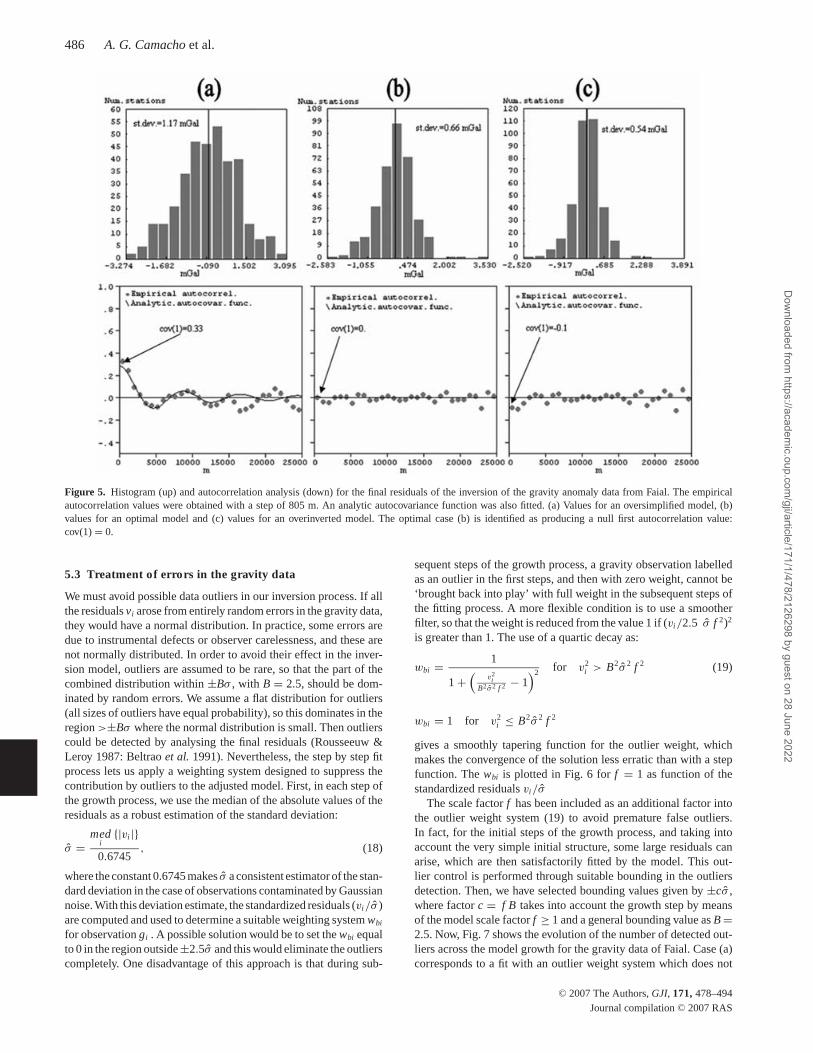
Fig. 5 displays a covariance analysis for the residuals of the Faialinversion. Part (a) corresponds to the final residuals of an insuffi-ciently developed model in which a correlated residual signal wasobserved. Case (b) corresponds to the optimum case of uncorre-lated residuals. Case (c) corresponds to the final residuals of anoverinverted model.

During the analysis, as the identifying characteristic parameterwe choose the covariance at null distance C(0), or else, for en-hanced computational simplicity, its approximation by means of thefirst empirical covariance, cov(d1). Therefore, the λ0 value for theoptimal model will correspond to a null value of C(0) ≡ cov(d1).

C© 2007 The Authors, GJI, 171, 478–494


Dow




Figure 5. Histogram (up) and autocorrelation analysis (down) for the final residuals of the inversion of the gravity anomaly data from Faial. The empiricalautocorrelation values were obtained with a step of 805 m. An analytic autocovariance function was also fitted. (a) Values for an oversimplified model, (b)values for an optimal model and (c) values for an overinverted model. The optimal case (b) is identified as producing a null first autocorrelation value:cov(1) = 0.

5.3 Treatment of errors in the gravity data

We must avoid possible data outliers in our inversion process. If allthe residuals vi arose from entirely random errors in the gravity data,they would have a normal distribution. In practice, some errors aredue to instrumental defects or observer carelessness, and these arenot normally distributed. In order to avoid their effect in the inver-sion model, outliers are assumed to be rare, so that the part of thecombined distribution within ±Bσ , with B = 2.5, should be dom-inated by random errors. We assume a flat distribution for outliers(all sizes of outliers have equal probability), so this dominates in theregion >±Bσ where the normal distribution is small. Then outlierscould be detected by analysing the final residuals (Rousseeuw &Leroy 1987: Beltrao et al. 1991). Nevertheless, the step by step fitprocess lets us apply a weighting system designed to suppress thecontribution by outliers to the adjusted model. First, in each step ofthe growth process, we use the median of the absolute values of theresiduals as a robust estimation of the standard deviation:

σ =med

i{|vi |}

0.6745, (18)

where the constant 0.6745 makes σ a consistent estimator of the stan-dard deviation in the case of observations contaminated by Gaussiannoise. With this deviation estimate, the standardized residuals (vi/σ )are computed and used to determine a suitable weighting system wbi

for observation gi . A possible solution would be to set the wbi equalto 0 in the region outside ±2.5σ and this would eliminate the outlierscompletely. One disadvantage of this approach is that during sub-

sequent steps of the growth process, a gravity observation labelledas an outlier in the first steps, and then with zero weight, cannot be‘brought back into play’ with full weight in the subsequent steps ofthe fitting process. A more flexible condition is to use a smootherfilter, so that the weight is reduced from the value 1 if (vi/2.5 σ f 2)2

is greater than 1. The use of a quartic decay as:

wbi = 1

1 +(

v2i

B2 σ 2 f 2 − 1)2 for v2

i > B2σ 2 f 2 (19)

wbi = 1 for v2i ≤ B2σ 2 f 2

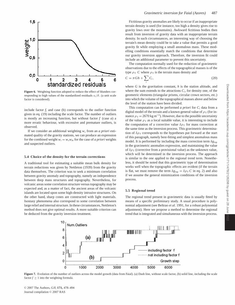
gives a smoothly tapering function for the outlier weight, whichmakes the convergence of the solution less erratic than with a stepfunction. The wbi is plotted in Fig. 6 for f = 1 as function of thestandardized residuals vi/σ

The scale factor f has been included as an additional factor intothe outlier weight system (19) to avoid premature false outliers.In fact, for the initial steps of the growth process, and taking intoaccount the very simple initial structure, some large residuals canarise, which are then satisfactorily fitted by the model. This out-lier control is performed through suitable bounding in the outliersdetection. Then, we have selected bounding values given by ±cσ ,where factor c = f B takes into account the growth step by meansof the model scale factor f ≥ 1 and a general bounding value as B =2.5. Now, Fig. 7 shows the evolution of the number of detected out-liers across the model growth for the gravity data of Faial. Case (a)corresponds to a fit with an outlier weight system which does not

C© 2007 The Authors, GJI, 171, 478–494


Dow




Figure 6. Weighting function adopted to reduce the effect of blunders cor-responding to high values of the standardized residuals vi /σ . (a unit scalefactor is considered).

include factor f, and case (b) corresponds to the outlier functiongiven in eq. (19) including the scale factor. The number of outliersis mostly an increasing function, but without factor f (case a) amore erratic behaviour, with excessive and premature outliers, isobserved.

If we consider an additional weighting ws from an a priori esti-mated quality of the gravity stations, we can produce an expressionfor the combined weight wi = wswbi for the case of a priori weightsand suspected outliers.

5.4 Choice of the density for the terrain corrections

A traditional tool for estimating a suitable mean bulk density forterrain reductions was given by Nettleton (1939) from the gravitydata themselves. The criterion was to seek a minimum correlationbetween gravity anomaly and topography, namely an independencebetween deep mass structures and topography. Nevertheless, forvolcanic areas some correlation structure versus topography may beexpected and, as a matter of fact, the ancient areas of the volcanicislands are located upon some high-density intrusive structures. Onthe other hand, sharp cones are constructed with light materials.Isostasy phenomena also correspond to some correlation betweenlarge relief and internal structure. In these circumstances, Nettleton’smethod does not give optimal results. A more suitable criterion canbe deduced from the gravity inversion treatment.

Fictitious gravity anomalies are likely to occur if an inappropriateterrain density is used (for instance, too high a density gives rise togravity lows over the mountains). Awkward fictitious bodies thenresult from inversion of gravity data with an inappropriate terraindensity. In such circumstances, an interesting way of choosing theterrain’s mean density could be to take a value that permits a goodgravity fit while employing a small anomalous mass. These mod-elling conditions essentially match the conditions that determineour gravity inversion approach. Therefore, the inversion fit couldinclude an additional parameter to prevent this uncertainty.

The computation normally used for the reduction of gravimetricobservations due to the effects of the topographical masses is of thetype ρT C where ρT is the terrain mass density and

C = πGh +∑

i

Ci , (20)

where G is the gravitation constant, h is the station altitude, andwhere the sum extends to the attractions Ci, for density one, of thegeometric elements (triangular prisms, circular crown sectors, etc.)into which the volume of the topographical masses above and belowthe level of the station have been divided.

This computation can be performed a priori for Ci data from adigital model of the terrain and a known general value of ρT (for in-stance ρT = 2670 kg m–3). However, due to the possible uncertaintyof the value ρT as a local suitable value, it is interesting to includethe computation of a corrective value δρT for mass correction atthe same time as the inversion process. This gravimetric determina-tion of δρT corresponds to the hypotheses put forward at the startof this paragraph, namely best-fitting and simplest anomalous massmodel. It is performed by including the mass correction term δg top

in the gravimetric anomalies expression, and maintaining the valueof δρT (corrective from a provisional value) as the unknown value,which will be determined in the inversion process. The approachis similar to the one applied to the regional trend term. Nonethe-less, it should be noted that this gravimetric type of determinationworks well when the topographic effects are evident (if the terrainis flat, we must remove the term δg top = δρT C in eq. 2) and alsoif we assume the general minimization conditions of the inversionprocess.

5.5 Regional trend

The regional trend present in gravimetric data is usually fitted bymeans of a specific preliminary study. A usual procedure is poly-nomial adjustment (see Beltrao et al. 1991, for a robust polynomialadjustment). Here we propose a method to determine the regionaltrend that is integrated and simultaneous with the inversion process.

Figure 7. Evolution of the number of outliers across the model growth (data from Faial). (a) Dash line, without scale factor, (b) solid line, including the scalefactor f ≥ 1 into the weighting formula.

C© 2007 The Authors, GJI, 171, 478–494


Dow




Perhaps the main problem lies in the exact definition of the re-gional trend. In this simultaneous adjustment (for inversion model,regional trend, terrain density and observational noise), the regionalcomponent of the anomalies is conceived as that part of the datawhich, due mainly to its long wavelength, cannot be modelled withthe volume elements predicted by the model. Therefore, the regionalcondition is of the ‘negative’ type: non-local, non-adjustable to thelocal structures in play. This condition can only be met in a simul-taneous fit. (Under these circumstances, and as we will see in thesimulation section, there may be a certain exchange between theregional component and the anomalies due to the model’s deeperstructures.)

Here we have used a linear representation δg reg = p0 + px(xi −xM ) + py(yi − yM ), i = 1, . . . , n, of the regional component, tosimplify the method’s formulism. p0 is a constant base and px, py

are SN and WE horizontal gradients. With a little more hard work,it is possible to develop, for example, the second degree formula.

5.6 Estimation of the precision for the adjustedparameters

As useful information, we can calculate values for the estimatedprecision of the parameters resulting for the inversion approach(anomalous density distribution, regional trend and correction forthe terrain density). For that, we write eqs (2) and (8) as:

d = G p − v, (21)

where d = (�g1. . .�gn)T is the data vector, p = (�ρ 11 , . . . ,�ρm, p0, px , py, δρT)T is composed by the model parameters (m

and the trend and terrain parameters) and G is the n × m matrixfor these linear equations (with n < m) as extension of matrix A.The covariance matrix for the data vector d is again QD, but nowthe covariance matrix QP for the parameters p can be obtained frommatrix λQM by adding the a priori variances for p0, px, py and ερT.Then, the posterior covariance matrix QP for parameters p can beobtained as (Tarantola 1988):

QP′ = QP − QPGT(GQ

PGT + QD

)−1GQP (22)

6 S I M U L AT I O N T E S T

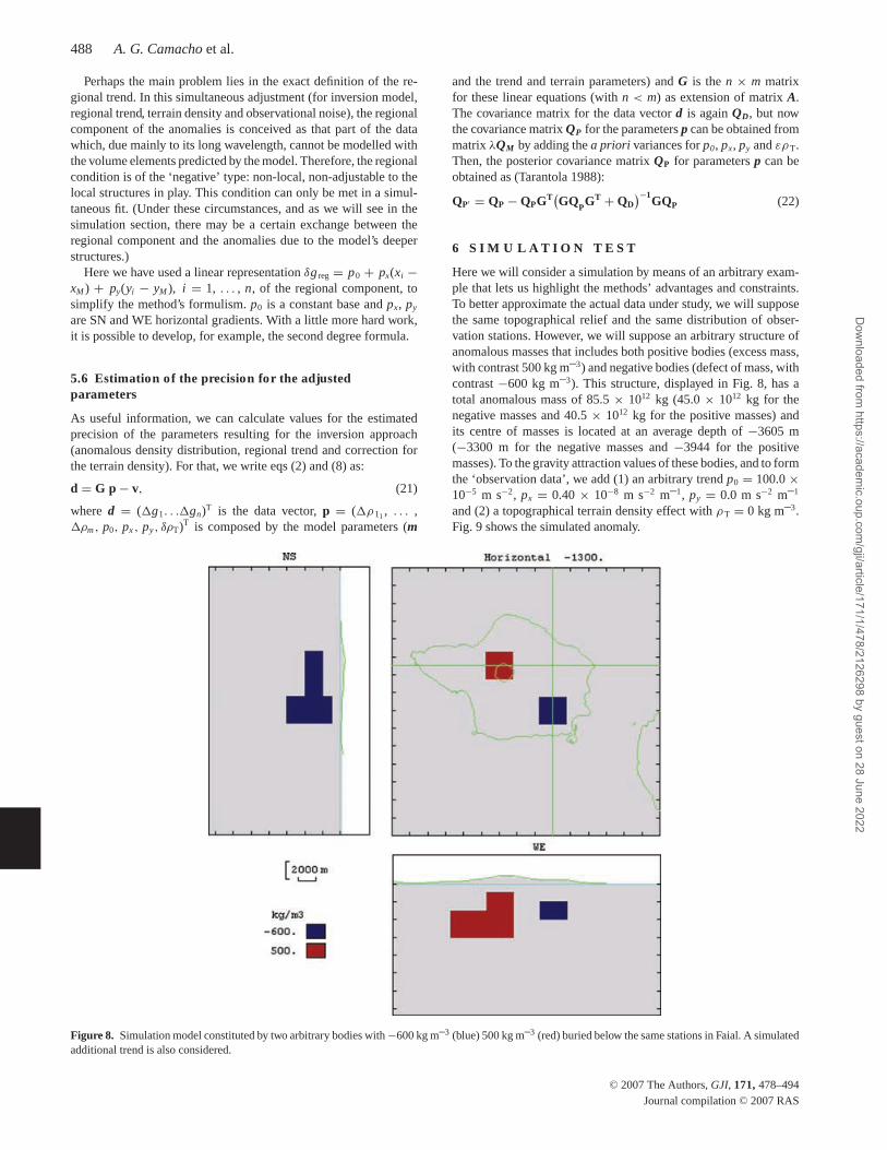
Here we will consider a simulation by means of an arbitrary exam-ple that lets us highlight the methods’ advantages and constraints.To better approximate the actual data under study, we will supposethe same topographical relief and the same distribution of obser-vation stations. However, we will suppose an arbitrary structure ofanomalous masses that includes both positive bodies (excess mass,with contrast 500 kg m–3) and negative bodies (defect of mass, withcontrast −600 kg m–3). This structure, displayed in Fig. 8, has atotal anomalous mass of 85.5 × 1012 kg (45.0 × 1012 kg for thenegative masses and 40.5 × 1012 kg for the positive masses) andits centre of masses is located at an average depth of −3605 m(−3300 m for the negative masses and −3944 for the positivemasses). To the gravity attraction values of these bodies, and to formthe ‘observation data’, we add (1) an arbitrary trend p0 = 100.0 ×10−5 m s−2, px = 0.40 × 10−8 m s−2 m–1, py = 0.0 m s−2 m–1

and (2) a topographical terrain density effect with ρT = 0 kg m–3.Fig. 9 shows the simulated anomaly.

Figure 8. Simulation model constituted by two arbitrary bodies with −600 kg m–3 (blue) 500 kg m–3 (red) buried below the same stations in Faial. A simulatedadditional trend is also considered.

C© 2007 The Authors, GJI, 171, 478–494


Dow




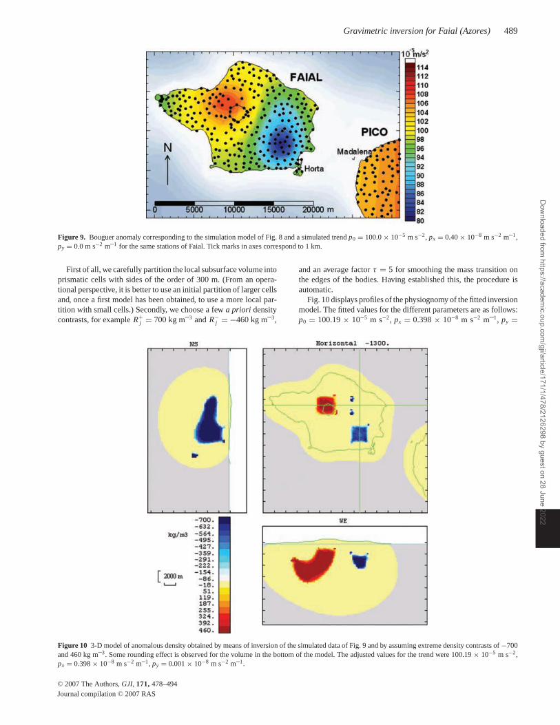
Figure 9. Bouguer anomaly corresponding to the simulation model of Fig. 8 and a simulated trend p0 = 100.0 × 10−5 m s−2, px = 0.40 × 10−8 m s−2 m–1,py = 0.0 m s−2 m–1 for the same stations of Faial. Tick marks in axes correspond to 1 km.

First of all, we carefully partition the local subsurface volume intoprismatic cells with sides of the order of 300 m. (From an opera-tional perspective, it is better to use an initial partition of larger cellsand, once a first model has been obtained, to use a more local par-tition with small cells.) Secondly, we choose a few a priori densitycontrasts, for example R+

j = 700 kg m–3 and R−j = −460 kg m–3,

and an average factor τ = 5 for smoothing the mass transition onthe edges of the bodies. Having established this, the procedure isautomatic.

Fig. 10 displays profiles of the physiognomy of the fitted inversionmodel. The fitted values for the different parameters are as follows:p0 = 100.19 × 10−5 m s−2, px = 0.398 × 10−8 m s−2 m–1, py =

Figure 10 3-D model of anomalous density obtained by means of inversion of the simulated data of Fig. 9 and by assuming extreme density contrasts of −700and 460 kg m–3. Some rounding effect is observed for the volume in the bottom of the model. The adjusted values for the trend were 100.19 × 10−5 m s−2,px = 0.398 × 10−8 m s−2 m–1, py = 0.001 × 10−8 m s−2 m–1.

C© 2007 The Authors, GJI, 171, 478–494


Dow




0.001 × 10−8 m s−2 m–1, ρT = 1 kg m–3, σ = 0.003 × 10−5 m s−2,total anomalous mass = 81.7 × 1012 kg, negative = 43.7 × 1012 kg,positive = 38.0 × 1012 kg, total average depth = −3510 m, negativemasses = −3257 m and positive masses = −3801 m. We see that,for this case of no errors, results are quite good.

Now we simulate an observational noise by adding a Gaussiannoise of arbitrary standard deviation 0.300 × 10−5 m s−2 (5 per centfrom the data variance) to the previous simulated data. Moreover, weinclude in the data three arbitrary outlier values. This additional dis-tortion produces a distortion and a reduction of the inverse model. Infact, the basic covariance sampling distance is �d = 805 m, which,as we indicated earlier, is the mean of the distances between neigh-bouring points. It provides us the estimation of a balance parameterfor the inversion. By applying the inversion process, now we obtain:p0 = 100.88 × 10−5 m s−2, px = 0.362 × 10−8 m s−2 m–1, py =0.043 × 10−8 m s−2 m–1, ρT = 42 kg m–3, not so good values asfor no observational errors. The resulting standard deviation of thefinal residual is σ = 0.3047 × 10−5 m s−2, quite similar to the sim-ulated one. Moreover, the three outlier data are clearly detected anddiscarded. The resulting 3-D model is significantly reduced (espe-cially in the deeper and less quality zones): total anomalous mass =66.1 × 1012 kg, negative = 44.0 × 1012 kg, positive = 28.1 × 1012

kg, total average depth = −3122 m, negative masses = −3148 mand positive masses = −3072 m.

The following comments may be made in view of these results.

1. The method works satisfactorily in the context of a fit withvery free conditions (no additional information or constraints) andlarge number of parameters.

2. As is generally predictable for potential fields, with uncertainsurface gravity data, it is almost impossible to fully reproduce thedeep structure (except with very exhaustive additional information),and especially in cases such as this that consider models that includeboth excesses and defects of mass.

3. Also predictably, it is observed that the model tends to‘smooth’ the corners. This smoothing effect is evidently greaterin the deeper areas than in the shallow ones.

4. The presence of observational noise produces some distortionand reduction of the model, mostly in the deeper and bad determinedzones.

7 I N V E R S I O N M O D E L F O R FA I A L A N DD I S C U S S I O N

The input gravity data is described in Section 3. There are not enoughprecise models about the inner structure of the island in the publishedliterature to be used as initial model for our inversion approach. Thenwe carried out a free adjustment corresponding to the observed grav-ity data. To that end, we considered a subsurface volume partitionwith cells of side ranging from 106 m for shallowest cells to 665 mfor the deepest cells (looking for a similar mean square effect onthe observation points). The maximum density contrast allowed was−400 and 300 kg m–3 everywhere, and the smoothness coefficientwas τ = 5 (see eq. 14).

After testing several tentative inversion models, we obtained (seeFig. 5) a suitable parameter λ0 for optimal balance between modelfitness and model magnitude according the proposed methodology.The inversion process simultaneously determined: a linear regionaltrend for the gravity data described by a decreasing rate of 0.59 ×10−8 m s−2 m–1 towards the southwest extreme (N224◦E), a terraindensity of 2341 kg m–3, a data noise level of 0.59 × 10−5 m s−2,and an anomalous model with mean density contrasts of −347

and 268 kg m–3. The estimated error values for these parameterswere ±147 × 10−5 m s−2, ±22 × 10−8 m s−2 m–1 and ±42 ×10−8 m s−2 m–1 for the components p0, px and py of the trend,±21 kg m–3 for the terrain density and a mean value of ±92 kg m–3

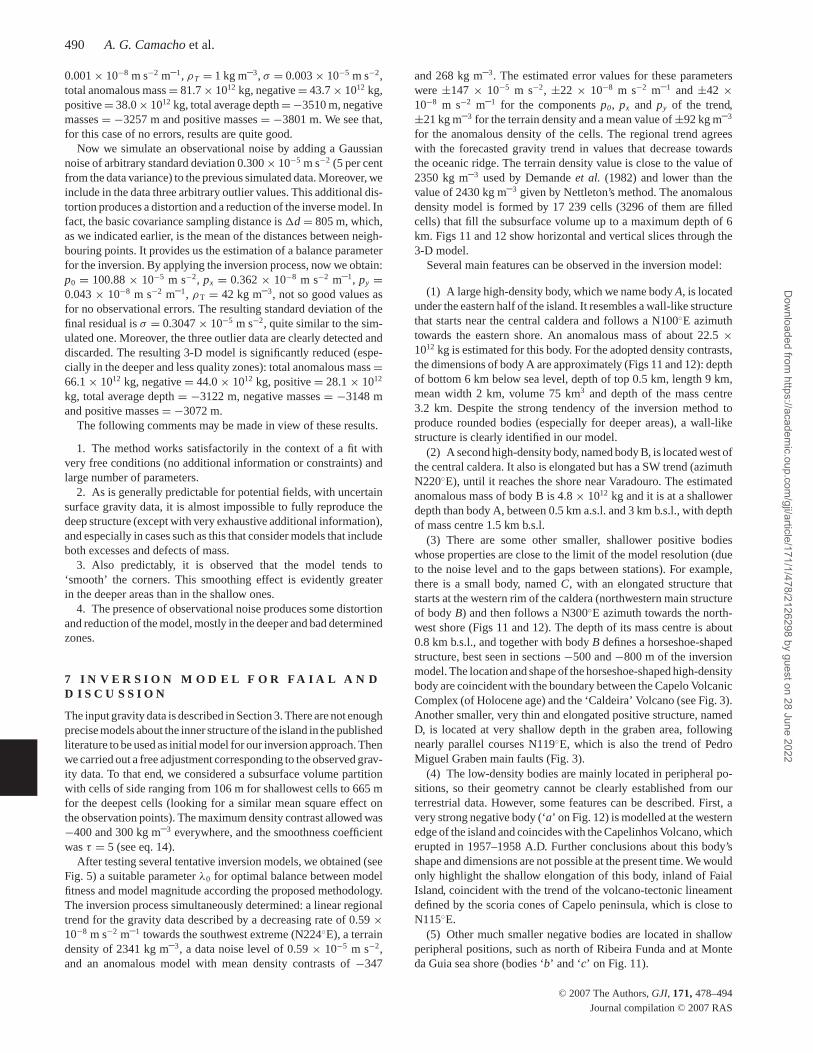
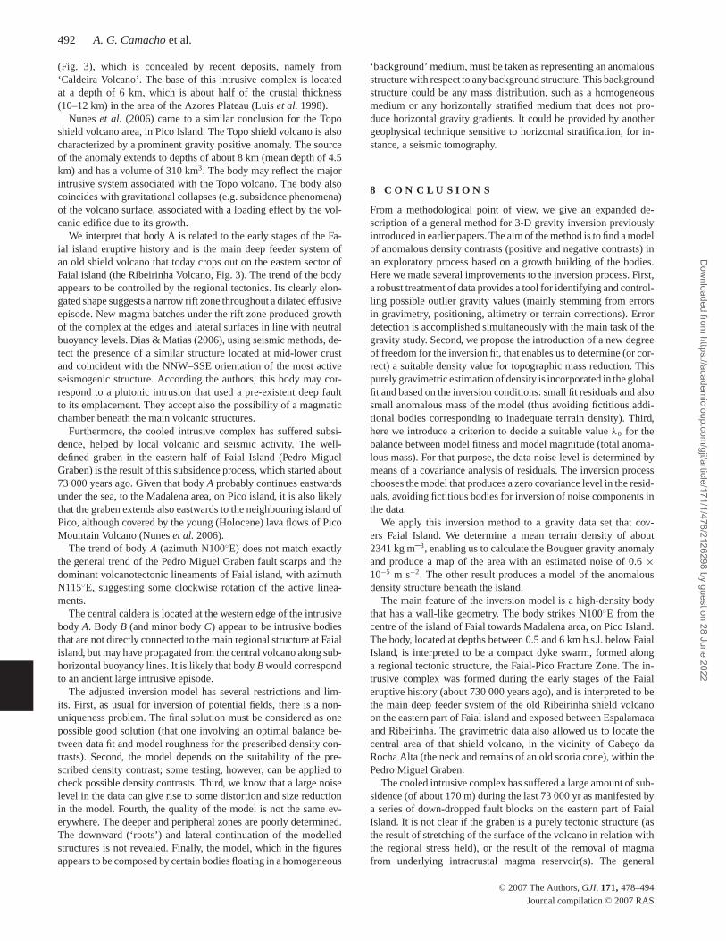
for the anomalous density of the cells. The regional trend agreeswith the forecasted gravity trend in values that decrease towardsthe oceanic ridge. The terrain density value is close to the value of2350 kg m–3 used by Demande et al. (1982) and lower than thevalue of 2430 kg m–3 given by Nettleton’s method. The anomalousdensity model is formed by 17 239 cells (3296 of them are filledcells) that fill the subsurface volume up to a maximum depth of 6km. Figs 11 and 12 show horizontal and vertical slices through the3-D model.

Several main features can be observed in the inversion model:

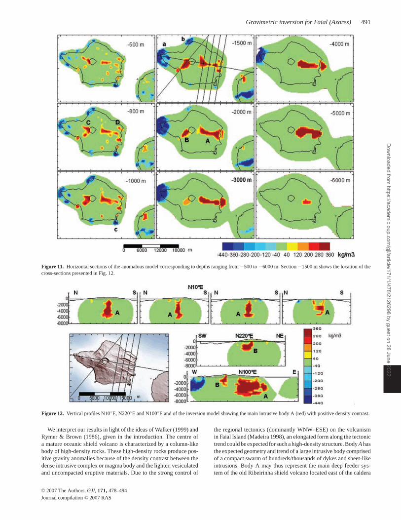
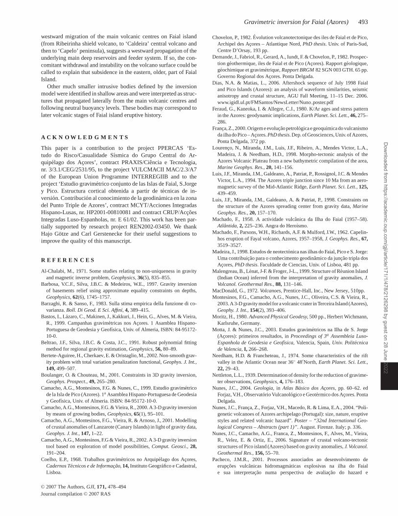
(1) A large high-density body, which we name body A, is locatedunder the eastern half of the island. It resembles a wall-like structurethat starts near the central caldera and follows a N100◦E azimuthtowards the eastern shore. An anomalous mass of about 22.5 ×1012 kg is estimated for this body. For the adopted density contrasts,the dimensions of body A are approximately (Figs 11 and 12): depthof bottom 6 km below sea level, depth of top 0.5 km, length 9 km,mean width 2 km, volume 75 km3 and depth of the mass centre3.2 km. Despite the strong tendency of the inversion method toproduce rounded bodies (especially for deeper areas), a wall-likestructure is clearly identified in our model.

(2) A second high-density body, named body B, is located west ofthe central caldera. It also is elongated but has a SW trend (azimuthN220◦E), until it reaches the shore near Varadouro. The estimatedanomalous mass of body B is 4.8 × 1012 kg and it is at a shallowerdepth than body A, between 0.5 km a.s.l. and 3 km b.s.l., with depthof mass centre 1.5 km b.s.l.

(3) There are some other smaller, shallower positive bodieswhose properties are close to the limit of the model resolution (dueto the noise level and to the gaps between stations). For example,there is a small body, named C, with an elongated structure thatstarts at the western rim of the caldera (northwestern main structureof body B) and then follows a N300◦E azimuth towards the north-west shore (Figs 11 and 12). The depth of its mass centre is about0.8 km b.s.l., and together with body B defines a horseshoe-shapedstructure, best seen in sections −500 and −800 m of the inversionmodel. The location and shape of the horseshoe-shaped high-densitybody are coincident with the boundary between the Capelo VolcanicComplex (of Holocene age) and the ‘Caldeira’ Volcano (see Fig. 3).Another smaller, very thin and elongated positive structure, namedD, is located at very shallow depth in the graben area, followingnearly parallel courses N119◦E, which is also the trend of PedroMiguel Graben main faults (Fig. 3).

(4) The low-density bodies are mainly located in peripheral po-sitions, so their geometry cannot be clearly established from ourterrestrial data. However, some features can be described. First, avery strong negative body (‘a’ on Fig. 12) is modelled at the westernedge of the island and coincides with the Capelinhos Volcano, whicherupted in 1957–1958 A.D. Further conclusions about this body’sshape and dimensions are not possible at the present time. We wouldonly highlight the shallow elongation of this body, inland of FaialIsland, coincident with the trend of the volcano-tectonic lineamentdefined by the scoria cones of Capelo peninsula, which is close toN115◦E.

(5) Other much smaller negative bodies are located in shallowperipheral positions, such as north of Ribeira Funda and at Monteda Guia sea shore (bodies ‘b’ and ‘c’ on Fig. 11).

C© 2007 The Authors, GJI, 171, 478–494


Dow




Figure 11. Horizontal sections of the anomalous model corresponding to depths ranging from −500 to −6000 m. Section −1500 m shows the location of thecross-sections presented in Fig. 12.

Figure 12. Vertical profiles N10◦E, N220◦E and N100◦E and of the inversion model showing the main intrusive body A (red) with positive density contrast.

We interpret our results in light of the ideas of Walker (1999) andRymer & Brown (1986), given in the introduction. The centre ofa mature oceanic shield volcano is characterized by a column-likebody of high-density rocks. These high-density rocks produce pos-itive gravity anomalies because of the density contrast between thedense intrusive complex or magma body and the lighter, vesiculatedand uncompacted eruptive materials. Due to the strong control of

the regional tectonics (dominantly WNW–ESE) on the volcanismin Faial Island (Madeira 1998), an elongated form along the tectonictrend could be expected for such a high-density structure. Body A hasthe expected geometry and trend of a large intrusive body comprisedof a compact swarm of hundreds/thousands of dykes and sheet-likeintrusions. Body A may thus represent the main deep feeder sys-tem of the old Ribeirinha shield volcano located east of the caldera

C© 2007 The Authors, GJI, 171, 478–494


Dow




(Fig. 3), which is concealed by recent deposits, namely from‘Caldeira Volcano’. The base of this intrusive complex is locatedat a depth of 6 km, which is about half of the crustal thickness(10–12 km) in the area of the Azores Plateau (Luis et al. 1998).

Nunes et al. (2006) came to a similar conclusion for the Toposhield volcano area, in Pico Island. The Topo shield volcano is alsocharacterized by a prominent gravity positive anomaly. The sourceof the anomaly extends to depths of about 8 km (mean depth of 4.5km) and has a volume of 310 km3. The body may reflect the majorintrusive system associated with the Topo volcano. The body alsocoincides with gravitational collapses (e.g. subsidence phenomena)of the volcano surface, associated with a loading effect by the vol-canic edifice due to its growth.

We interpret that body A is related to the early stages of the Fa-ial island eruptive history and is the main deep feeder system ofan old shield volcano that today crops out on the eastern sector ofFaial island (the Ribeirinha Volcano, Fig. 3). The trend of the bodyappears to be controlled by the regional tectonics. Its clearly elon-gated shape suggests a narrow rift zone throughout a dilated effusiveepisode. New magma batches under the rift zone produced growthof the complex at the edges and lateral surfaces in line with neutralbuoyancy levels. Dias & Matias (2006), using seismic methods, de-tect the presence of a similar structure located at mid-lower crustand coincident with the NNW–SSE orientation of the most activeseismogenic structure. According the authors, this body may cor-respond to a plutonic intrusion that used a pre-existent deep faultto its emplacement. They accept also the possibility of a magmaticchamber beneath the main volcanic structures.

Furthermore, the cooled intrusive complex has suffered subsi-dence, helped by local volcanic and seismic activity. The well-defined graben in the eastern half of Faial Island (Pedro MiguelGraben) is the result of this subsidence process, which started about73 000 years ago. Given that body A probably continues eastwardsunder the sea, to the Madalena area, on Pico island, it is also likelythat the graben extends also eastwards to the neighbouring island ofPico, although covered by the young (Holocene) lava flows of PicoMountain Volcano (Nunes et al. 2006).

The trend of body A (azimuth N100◦E) does not match exactlythe general trend of the Pedro Miguel Graben fault scarps and thedominant volcanotectonic lineaments of Faial island, with azimuthN115◦E, suggesting some clockwise rotation of the active linea-ments.

The central caldera is located at the western edge of the intrusivebody A. Body B (and minor body C) appear to be intrusive bodiesthat are not directly connected to the main regional structure at Faialisland, but may have propagated from the central volcano along sub-horizontal buoyancy lines. It is likely that body B would correspondto an ancient large intrusive episode.

The adjusted inversion model has several restrictions and lim-its. First, as usual for inversion of potential fields, there is a non-uniqueness problem. The final solution must be considered as onepossible good solution (that one involving an optimal balance be-tween data fit and model roughness for the prescribed density con-trasts). Second, the model depends on the suitability of the pre-scribed density contrast; some testing, however, can be applied tocheck possible density contrasts. Third, we know that a large noiselevel in the data can give rise to some distortion and size reductionin the model. Fourth, the quality of the model is not the same ev-erywhere. The deeper and peripheral zones are poorly determined.The downward (‘roots’) and lateral continuation of the modelledstructures is not revealed. Finally, the model, which in the figuresappears to be composed by certain bodies floating in a homogeneous

‘background’ medium, must be taken as representing an anomalousstructure with respect to any background structure. This backgroundstructure could be any mass distribution, such as a homogeneousmedium or any horizontally stratified medium that does not pro-duce horizontal gravity gradients. It could be provided by anothergeophysical technique sensitive to horizontal stratification, for in-stance, a seismic tomography.

8 C O N C L U S I O N S

From a methodological point of view, we give an expanded de-scription of a general method for 3-D gravity inversion previouslyintroduced in earlier papers. The aim of the method is to find a modelof anomalous density contrasts (positive and negative contrasts) inan exploratory process based on a growth building of the bodies.Here we made several improvements to the inversion process. First,a robust treatment of data provides a tool for identifying and control-ling possible outlier gravity values (mainly stemming from errorsin gravimetry, positioning, altimetry or terrain corrections). Errordetection is accomplished simultaneously with the main task of thegravity study. Second, we propose the introduction of a new degreeof freedom for the inversion fit, that enables us to determine (or cor-rect) a suitable density value for topographic mass reduction. Thispurely gravimetric estimation of density is incorporated in the globalfit and based on the inversion conditions: small fit residuals and alsosmall anomalous mass of the model (thus avoiding fictitious addi-tional bodies corresponding to inadequate terrain density). Third,here we introduce a criterion to decide a suitable value λ0 for thebalance between model fitness and model magnitude (total anoma-lous mass). For that purpose, the data noise level is determined bymeans of a covariance analysis of residuals. The inversion processchooses the model that produces a zero covariance level in the resid-uals, avoiding fictitious bodies for inversion of noise components inthe data.

We apply this inversion method to a gravity data set that cov-ers Faial Island. We determine a mean terrain density of about2341 kg m–3, enabling us to calculate the Bouguer gravity anomalyand produce a map of the area with an estimated noise of 0.6 ×10−5 m s−2. The other result produces a model of the anomalousdensity structure beneath the island.

The main feature of the inversion model is a high-density bodythat has a wall-like geometry. The body strikes N100◦E from thecentre of the island of Faial towards Madalena area, on Pico Island.The body, located at depths between 0.5 and 6 km b.s.l. below FaialIsland, is interpreted to be a compact dyke swarm, formed alonga regional tectonic structure, the Faial-Pico Fracture Zone. The in-trusive complex was formed during the early stages of the Faialeruptive history (about 730 000 years ago), and is interpreted to bethe main deep feeder system of the old Ribeirinha shield volcanoon the eastern part of Faial island and exposed between Espalamacaand Ribeirinha. The gravimetric data also allowed us to locate thecentral area of that shield volcano, in the vicinity of Cabeco daRocha Alta (the neck and remains of an old scoria cone), within thePedro Miguel Graben.

The cooled intrusive complex has suffered a large amount of sub-sidence (of about 170 m) during the last 73 000 yr as manifested bya series of down-dropped fault blocks on the eastern part of FaialIsland. It is not clear if the graben is a purely tectonic structure (asthe result of stretching of the surface of the volcano in relation withthe regional stress field), or the result of the removal of magmafrom underlying intracrustal magma reservoir(s). The general

C© 2007 The Authors, GJI, 171, 478–494


Dow




westward migration of the main volcanic centres on Faial island(from Ribeirinha shield volcano, to ‘Caldeira’ central volcano andthen to ‘Capelo’ peninsula), suggests a westward propagation of theunderlying main deep reservoirs and feeder system. If so, the con-comitant withdrawal and instability on the volcano surface could becalled to explain that subsidence in the eastern, older, part of FaialIsland.

Other much smaller intrusive bodies defined by the inversionmodel were identified in shallow areas and were interpreted as struc-tures that propagated laterally from the main volcanic centres andfollowing neutral buoyancy levels. These bodies may correspond tolater volcanic stages of Faial island eruptive history.

A C K N O W L E D G M E N T S

This paper is a contribution to the project PPERCAS ‘Es-tudo do Risco/Casualidade Sısmica do Grupo Central do Ar-quipelago dos Acores’, contract PRAXIS/Ciencia e Tecnologia,nr. 3/3.1/CEG/2531/95, to the project VULCMACII MAC/2.3/A7of the European Union Programme INTERREGIIB and to theproject ‘Estudio gravimetrico conjunto de las Islas de Faial, S.Jorgey Pico. Estructura cortical obtenida a partir de tecnicas de in-version. Contribucion al conocimiento de la geodinamica en la zonadel Punto Triple de Azores’, contract MCYT/Acciones IntegradasHispano-Lusas, nr. HP2001-00810081 and contract CRUP/AccoesIntegradas Luso-Espanholas, nr. E 61/02. This work has been par-tially supported by research project REN2002-03450. We thankHajo Gotze and Carl Gerstenecke for their useful suggestions toimprove the quality of this manuscript.

R E F E R E N C E S

Al-Chalabi, M., 1971. Some studies relating to non-uniqueness in gravityand magnetic inverse problem, Geophysics, 36(5), 835–855.

Barbosa, V.C.F., Silva, J.B.C. & Medeiros, W.E., 1997. Gravity inversionof basements relief using approximate equality constraints on depths,Geophysics, 62(6), 1745–1757.

Barzaghi, R. & Sanso, F., 1983. Sulla stima empirica della funzione di co-varianza. Boll. Di Geod. E Sci. Affini, 4, 389–415.

Bastos, L, Lazaro, C., Makinen, J., Kakkuri, J., Hein, G., Alves, M. & Vieira,R., 1999. Campanhas gravimetricas nos Acores. 1 Asamblea Hispano-Portuguesa de Geodesia y Geofısica, Univ. of Almeria, ISBN: 84-95172-10-0.

Beltrao, J.F., Silva, J.B.C. & Costa, J.C., 1991. Robust polynomial fittingmethod for regional gravity estimation, Geophysics, 56, 80–89.

Bertete-Aguiree, H., Cherkaev, E. & Oristaglio, M., 2002. Non-smooth grav-ity problem with total variation penalization functional, Geophys. J. Int.,149, 499–507.

Boulanger, O. & Chouteau, M., 2001. Constraints in 3D gravity inversion,Geophys. Prospect., 49, 265–280.

Camacho, A.G., Montesinos, F.G. & Nunes, C., 1999. Estudio gravimetricode la Isla de Pico (Azores). 1a Asamblea Hispano-Portuguesa de Geodesiay Geofısica, Univ. of Almeria. ISBN: 84-95172-10-0.

Camacho, A.G., Montesinos, F.G. & Vieira, R., 2000. A 3-D gravity inversionby means of growing bodies, Geophysics, 65(1), 95–101.

Camacho, A.G., Montesinos, F.G., Vieira, R. & Arnoso, J., 2001. Modellingof crustal anomalies of Lanzarote (Canary Islands) in light of gravity data,Geophys. J. Int., 147, 1–22.

Camacho, A.G., Montesinos, F.G & Vieira, R., 2002. A 3-D gravity inversiontool based on exploration of model possibilities, Comput. Geosci., 28,191–204.

Coelho, E.P., 1968. Trabalhos gravimetricos no Arquipelago dos Acores,Cadernos Tecnicos e de Informacao, 14, Instituto Geografico e Cadastral,Lisboa.

Chovelon, P., 1982. Evolution volcanotectonique des iles de Faial et de Pico,Archipel des Acores – Atlantique Nord, PhD thesis. Univ. of Paris-Sud,Centre D’Orsay, 193 pp.

Demande, J., Fabriol, R., Gerard, A., Iundt, F. & Chovelon, P., 1982. Prospec-tion geothermique, iles de Faial et de Pico (Acores). Rapport geologique,geochimique et gravimetrique, Rapport BRGM 82 SGN 003 GTH. 65 pp.Governo Regional dos Acores. Ponta Delgada.

Dias, N.A. & Matias, L., 2006. Aftershock sequence of July 1998 Faialand Pico Islands (Azores): an analysis of waveform similarities, seismicanisotropy and crustal structure, AGU Fall Meeting, 11–15 Dec. 2006.www.igidl.ul.pt/FMSantos/NewsLetter/Nuno poster.pdf

Feraud, G., Kaneoka, I. & Allegre, C.J., 1980. K/Ar ages and stress patternin the Azores: geodynamic implications, Earth Planet. Sci. Lett., 46, 275–286.

Franca, Z., 2000. Origem e evolucao petrologica e geoquımica do vulcanismoda ilha do Pico – Acores. PhD thesis. Dep. of Geosciences, Univ. of Azores,Ponta Delgada, 372 pp.

Lourenco, N., Miranda, J.M., Luis, J.F., Ribeiro, A., Mendes Victor, L.A.,Madeira, J. & Needham, H.D., 1998. Morpho-tectonic analysis of theAzores Volcanic Plateau from a new bathymetric compilation of the area,Marine Geophys. Res., 20, 141–156.

Luis, J.F., Miranda, J.M., Galdeano, A., Patriat, P., Rossignol, J.C. & MendesVictor, L.A., 1994. The Azores triple junction since 10 Ma from an aero-magnetic survey of the Mid-Atlantic Ridge, Earth Planet. Sci. Lett., 125,439–459.

Luis, J.F., Miranda, J.M., Galdeano, A. & Patriat, P., 1998. Constraints onthe structure of the Azores spreading center from gravity data, MarineGeophys. Res., 20, 157–170.

Machado, F., 1958. A actividade vulcanica da Ilha do Faial (1957–58).Atlantida, 2, 225–236. Angra do Heroısmo.

Machado, F., Parsons, W.H., Richards, A.F. & Mulford, J.W., 1962. Capelin-hos eruption of Fayal volcano, Azores, 1957–1958, J. Geophys. Res., 67,3519–3527.

Madeira, J., 1998. Estudos de neotectonica nas ilhas do Faial, Pico e S. Jorge:Uma contribuicao para o conhecimento geodinamico da juncao tripla dosAcores, PhD thesis. Faculdade de Ciencias, Univ. of Lisboa, 481 pp.

Malengreau, B., Lenat, J-F. & Froger, J-L., 1999. Structure of Reunion Island(Indian Ocean) inferred from the interpretation of gravity anomalies, J.Volcanol. Geothermal Res., 88, 131–146.

MacDonald, G., 1972. Volcanoes, Prentice-Hall, Inc., New Jersey, 510pp.Montesinos, F.G., Camacho, A.G., Nunes, J.C., Oliveira, C.S. & Vieira, R.,

2003. A 3-D gravity model for a volcanic crater in Terceira Island (Azores),Geophy. J. Int., 154(2), 393–406.

Moritz, H., 1980. Advanced Physical Geodesy, 500 pp., Herbert Wichmann,Karlsruhe, Germany.

Motta, J. & Nunes, J.C., 2003. Estudos gravimetricos na Ilha de S. Jorge(Acores): primeiros resultados, in Proceedings of 3a Assembleia Luso-Espanhola de Geodesia e Geofısica, Valencia, Spain, Univ. Politecnicade Valencia, I, 266–268.

Needham, H.D. & Francheteau, J., 1974. Some characteristics of the riftvalley in the Atlantic Ocean near 36◦ 48′North, Earth Planet. Sci. Lett.,22, 29–43.

Nettleton, L.L., 1939. Determination of density for the reduction of gravime-ter observations, Geophysics, 4, 176–183.

Nunes, J.C., 2004. Geologia, in Atlas Basico dos Acores, pp. 60–62. edForjaz, V.H., Observatorio Vulcanologico e Geotermico dos Acores. PontaDelgada.

Nunes, J.C., Franca, Z., Forjaz, V.H., Macedo, R. & Lima, E.A., 2004. “Poli-genetic volcanoes of Azores archipelago (Portugal): size, nature, eruptivestyles and related volcanic hazard”. Poster – “32nd International Geo-logical Congress – Abstracts (part 1)”. August. Firenze. Italy; p. 336.

Nunes, J.C., Camacho, A.G., Franca, Z., Montesinos, F., Alves, M., Vieira,R., Velez, E. & Ortiz, E., 2006. Signature of crustal volcano-tectonicstructures of Pico island (Azores) based on gravity anomalies, J. Volcanol.Geothermal Res., 156, 55–70.

Pacheco, J.M.R., 2001. Processos associados ao desenvolvimento deerupcoes vulcanicas hidromagmaticas explosivas na ilha do Faiale sua interpretacao numa perspectiva de avaliacao do hazard e

C© 2007 The Authors, GJI, 171, 478–494


Dow




minimizacao do risco. PhD thesis. Azores University. Ponta Delgada.300 pp.

Pedersen, L.B., 1979. Constrained Inversion of Potential Field Data, Geo-phys. Prospect., 27, 726–748.

Pick, M., Picha, J. & Vyskocil, V., 1973. Theory of the Earths Gravity Field,Elsevier, New York, 538 pp.

Rene, R. M., 1986. Gravity inversion using open, reject, and “shape-of-anomaly” fill criteria, Geophysics, 51(4), 988–994.

Rousseeuw, P.J. & Leroy, A.M., 1987. Robust Regression and Outlier De-tection, John Wiley & Sons, New York, 327 pp.

Rymer, H. & Brown, G.C., 1986. Gravity fields and the interpretation ofvolcanic structures: geological discrimination and temporal evolution, J.Volcanol. Geotherm. Res., 27, 229–254.

Rothman, D.H., 1985. Nonlinear inversion, statistical mechanics, and resid-ual statics estimation, Geophysics, 50(12), 2784–2796.

Searle, R., 1980. Tectonic pattern of the Azores spreading centre and triplejunction, Earth Planet. Sci. Lett., 51, 415–434.

Serralheiro, A., Forjaz, V.H., Alves, C.A.M. & Rodrigues, B., 1989. CartaVulcanologica dos Acores-Ilha do Faial. Escala 1:15 000. Sheets 1, 2,

3 & 4. Centro de Vulcanologia do INIC, Servico Regional de ProteccaoCivil dos Acores & Univ. of Azores (Ed.), Ponta Delgada.

Silva, J.B.C. & Hohmann, G.W., 1983. Nonlinear magnetic inversion usinga random search method, Geophysics, 46(12), 1645–1658.

Smith, W.H.F. & Sandwell, D.T., 1997. Global sea floor topography fromsatellite altimetry and ship depth soundings, Science, 277, 1956–1962.

Tarantola, A., 1988. The Inverse Problem Theory: Methods for Data Fittingand Model Parameter Estimation, Elsevier, Amsterdam, 613 pp.

Tazieff, H., 1959. L’eruption de 1957–1958 et la tectonique de Faial(Acores), Memorias dos Servicos Geologicos de Portugal, 4, 71–88.

Tiede, C., Camacho, A.G., Gerstenecker, C., Fernandez, J., & Suyanto, I.,2005. Modelling the crust at Merapi volcano area, Indonesia, via the in-verse gravimetric problem.Geochemistry, Geophysics, Geosystems (G3),6, doi:10.1029/2005GC000986.

Walker, G.P.L., 1992. Coherent intrusion complexes in large basalticvolcanoes—a new structural model, J. Volcanol. Geotherm. Res., 50, 41–54.

Walker, G.P.L., 1999. Volcanic rift zones and their intrusion swarms, J. Vol-canol. Geotherm. Res., 94, 21–34.

C© 2007 The Authors, GJI, 171, 478–494


Dow



Documents

Gravimetric determination of an intrusive complex under the