Sovereign Credit Risk, Financial Fragility,

and Global Factors

Anusha Chari Felipe Garces Juan Francisco Martınez Patricio Valenzuela

December 10, 2020∗

Abstract

This study explores the relationship between sovereign credit risk, financial fragility,

and global factors in emerging market economies, by using a novel model-based

semi-parametric metric (JLoss) that computes the expected joint loss of the bank-

ing sector conditional on a systemic event. Our metric of financial fragility is

positively associated with sovereign bond spreads and negatively associated with

higher sovereign credit ratings, after controlling for the standard determinants of

sovereign credit risk. The results additionally indicate that countries with more

fragile banking sectors are more exposed to global (exogenous) financial factors

than those with more resilient banking sectors. These findings underscore that

regulators must ensure the stability of the banking sector to improve governments’

borrowing costs in international debt markets.

JEL Codes: E43, E44, F30, G12, G15.

Keywords: banks, credit ratings, credit risk, emerging economies, global factors.

∗Anusha Chari is at the University of North Carolina at Chapel Hill, Felipe Garces and Juan FranciscoMartinez are at the Central Bank of Chile, and Patricio Valenzuela is at the University of Chile. We wishto thank CAE Goodhart, Dimitrios Tsomocos, Jose Vicente Martinez, and Oren Sussman for insightfulcomments on an earlier version of this paper. We have benefited from helpful comments from participantsat the First Conference on Financial Stability and Sustainability.

1

1 Motivation

The global financial crisis of 2008-09 and the European debt crisis, which were char-

acterized by large losses in the banking sector, affected international debt markets

severely. They produced a significant deterioration of sovereign credit spreads and

ratings with the greater expectation of public support for distressed banks (Mody

and Sandri, 2012). Despite a rich body of research on the drivers of sovereign

credit risk, a better understanding of the factors influencing sovereign risk and

of how these factors can be properly measured in both advanced and emerging

economies is of key importance for several reasons. Sovereign credit risk is not

only a key determinant of governments’ borrowing costs, but also remains a sig-

nificant determinant of the cost of debt capital for the private sector (Cavallo and

Valenzuela, 2010; Borensztein, Cowan, and Valenzuela, 2013). Moreover, sovereign

credit risk directly influences the ability of investors to diversify the risk of global

debt portfolios and plays a crucial role in determining capital flows across countries

(Longstaff et al., 2011).

The literature has recently emphasized that the primary factors that affect

sovereign credit risk are macroeconomic fundamentals, global factors, and finan-

cial fragility, which have generally been treated as independent determinants of

sovereign credit risk. Although macroeconomic fundamentals have substantial ex-

planatory power for sovereign credit spreads in emerging economies (Hilscher and

Nosbusch, 2010), sovereign credit risk appears to be mainly driven by global fi-

nancial factors (Gonzalez-Rosada and Yeyati, 2008; Longstaff et al., 2011). Fi-

nancial fragility also seems to influence governments’ indebtedness and credit risk.

Greater banking-sector fragility predicts larger bank bailouts, larger public debt,

and higher sovereign credit risk (Acharya, Drechsler, and Schnabl, 2014; Kallestrup,

Lando, and Murgoci, 2016; Farhi and Tirole, 2018). This relationship between bank

risk and sovereign risk is particularly strong during periods of financial distress

(Fratzscher and Rieth, 2019). Finally, recent empirical evidence also suggests sys-

temic sovereign risk has its roots in financial markets rather than in macroeconomic

fundamentals (Dieckmann and Plank, 2012; Ang and Longstaff, 2013). Specifically,

Dieckmann and Plank (2012) show the state of the domestic financial market and

the state of the global financial system have strong explanatory power for the evo-

2

lution of sovereign spreads, and that the magnitude of the effect is shaped by the

importance of the domestic financial system pre-crisis.

Using a novel model-based semi-parametric metric (JLoss) that computes the

expected joint loss of the banking sector in the event of a large financial meltdown,

in this study, we explore the relationship between sovereign credit risk, financial

fragility, and global financial factors. We study this relationship in a panel data set

that covers 19 emerging market economies from 1999:Q1 to 2017:Q3. Consistent

with the idea that our metric (JLoss) can be understood as the direct cost of bail-

ing out the whole banking sector, and with recent evidence that shows sovereign

spreads increased in the eurozone with the greater expectation of public support for

distressed banks (Mody and Sandri, 2012), our results indicate our metric of finan-

cial fragility is positively associated with sovereign credit spreads and negatively

associated with higher sovereign credit ratings. The results additionally indicate

countries with more fragile banking sectors are more exposed to the influence of

global (exogenous) financial factors related to market volatility, risk-free interest

rates, risk premiums, and aggregate illiquidity. Our results are statistically signifi-

cant and economically meaningful, even after controlling for country and time fixed

effects, the standard determinants of sovereign credit risk, and systemic banking

crises. These findings underscore that the stability of the domestic banking sector

plays a crucial role in reducing sovereign risk and its exposure to global factors.

This study contributes to the literature in at least three ways. First, it intro-

duces a new measure of financial fragility in the banking sector (JLoss) that reflects

the expected joint loss of the domestic banking sector in the event of a large financial

meltdown. The calculation of our JLoss metric employs a saddle-point methodol-

ogy in which the distribution of potential losses in the banking system is a function

of the bank-specific probabilities of default, the exposure in case of default, a loss

given default (LGD) parameter, and the correlation between the banks’ stock mar-

ket returns and the stock market index returns of each country. Recent academic

studies have introduced measures of systemic risk (e.g., see Brownlees and Engle

(2016) for a measure of systemic risk for the U.S.). However, given that our metric

of the expected joint loss of the domestic banking sector can be interpreted as the

direct cost of bailing banks out from a crisis, it should be a particularly significant

3

factor to consider in the pricing of sovereign bonds.

Second, this study explores the relationship between sovereign credit risk and fi-

nancial fragility in a sample of emerging economies. Thus, this study is a departure

from recent studies that have focused their analysis on samples of European coun-

tries during the Eurozone sovereign and banking crises. Mody and Sandri (2012)

argue that sovereign credit spreads increased in the eurozone with the greater ex-

pectation of public support for distressed banks and that this effect was stronger

in countries with lower growth prospects and higher debt burdens. Fratzscher and

Rieth (2019) show the correlation between CDS spreads of European banks and

sovereigns rose from 0.1 in 2007 to 0.8 in 2013, and attribute this higher correlation

to a two-way causality between bank credit risk and sovereign credit risk. Although

the study of sovereign credit risk in emerging economies has received much atten-

tion (Boehmer and Megginson, 1990; Edwards, 1986; Hilscher and Nosbusch, 2010;

Longstaff et al., 2011), new research on the relationship between banking fragility

and sovereign credit risk in emerging economies has been sparse.

Third, this study takes an additional step beyond the extant literature by ex-

ploring a channel (i.e., the fragility of the banking sector) that amplifies the effect of

global (exogenous) factors on sovereign credit risk. Although global factors have re-

cently been viewed as push factors in the literature, they have usually been modeled

as having homogeneous effects on sovereign credit risk (see, e.g., Gonzalez-Rosada

and Yeyati, 2008). Our analysis suggests that regulations and policies aimed at

improving the stability of the domestic banking sector may be helpful in reducing

the exposure to global factors, which have become increasingly important in a more

financially integrated world.

The remainder of the article is organized as follows. Section 2 presents the JLoss

methodology utilized to construct a financial fragility measure. Section 3 describes

the sample and variables used in this study. Section 4 presents our empirical strat-

egy and reports the main results. Section 5 conducts a set of robustness checks.

Finally, section 6 concludes.

4

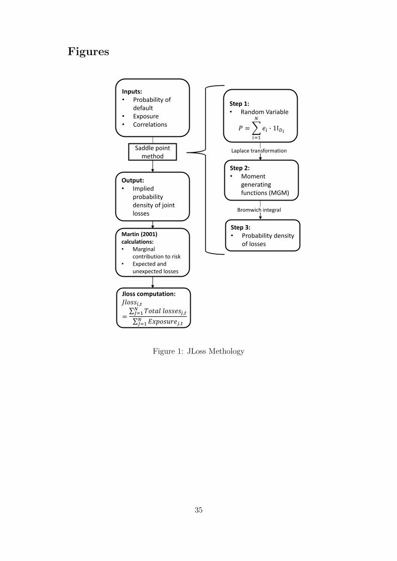
2 Joint Loss (JLoss) Measure

To study the relationship between financial fragility and sovereign credit risk, in

this work we construct a novel country-level metric of financial fragility (JLoss).

JLoss is a model-based semi-parametric metric of the joint loss of the banking

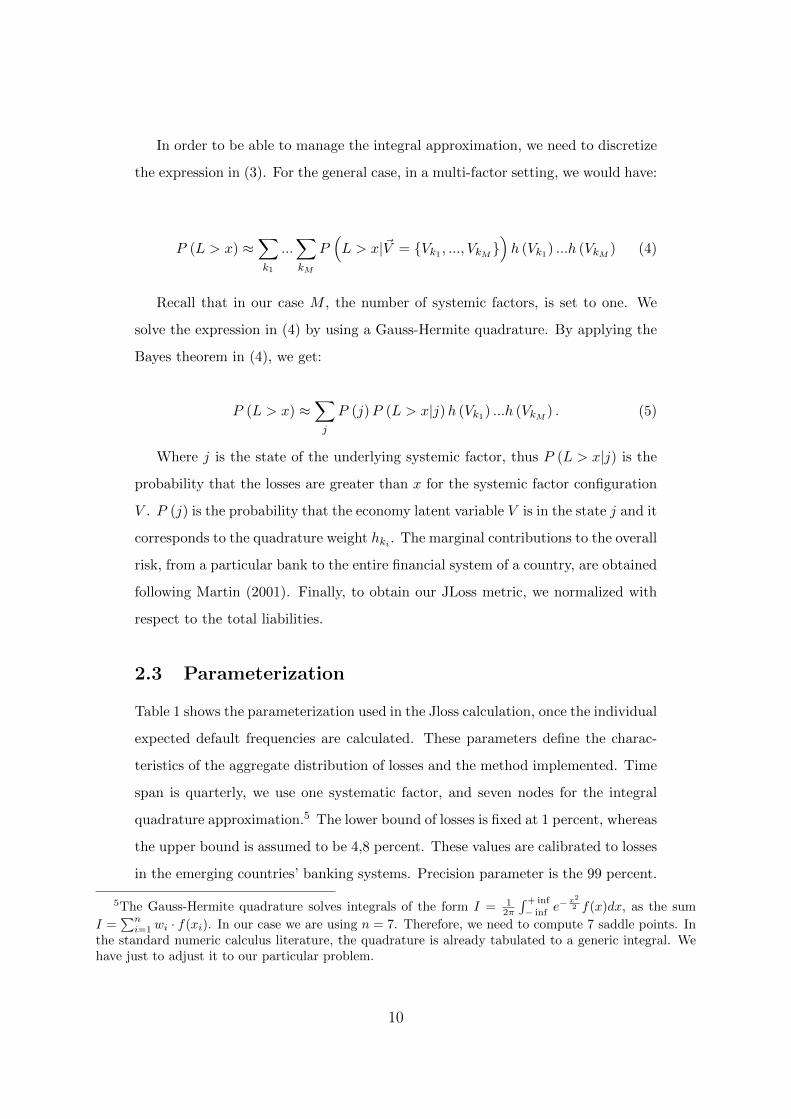
sector conditional on a systemic event. Figure 1 presents an overview of the JLoss

methodology.

To calculate our JLoss metric, we first employ a saddle-point methodology that

allows us to calculate the aggregated distribution of losses. In this approach the

distribution of potential losses in the banking system is a function of the banks’

probabilities and exposure at default, a loss given default (LGD) parameter, and

the correlation between banks’ stock market returns and a systemic component.

The individual probabilities of default are calculated following a modification of

the Merton’s (1974) model. The exposure is proxied by the amount of liabilities

of the banks at the moment of default. The LGD for banking debt is set to a

45%, as suggested by the Bank of International Settlements (BIS, 2006). The

key assumption in our approach is that bank risks are uncorrelated, conditional

on being correlated with a systemic factor, which in our case is the overall stock

market performance of each country. With the distribution of potential losses in

the banking system, we calculate each bank’s marginal contribution to the total

risk. Finally, we normalize these contributions to the total risk with respect to

total liabilities.

Next, we describe in detail the calculation of the banks’ default probabilities

and the aggregation of losses with the saddle-point method.

2.1 Individual Probabilities: Distance-to-Default

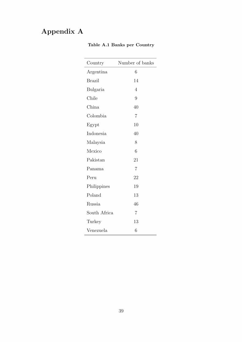
To calculate default probabilities for each bank, we employ Kealhofer’s (2000) ap-

proach. This approach is a standard modification of the structural credit risk model

introduced by Merton (1974). Table A.1 in the appendix reports the number of

banks used in our analyses by country.

Our measurement approach merges together information on banks’ balance

sheet and market prices: long and short term liabilities (LST , LLT ), short term

5

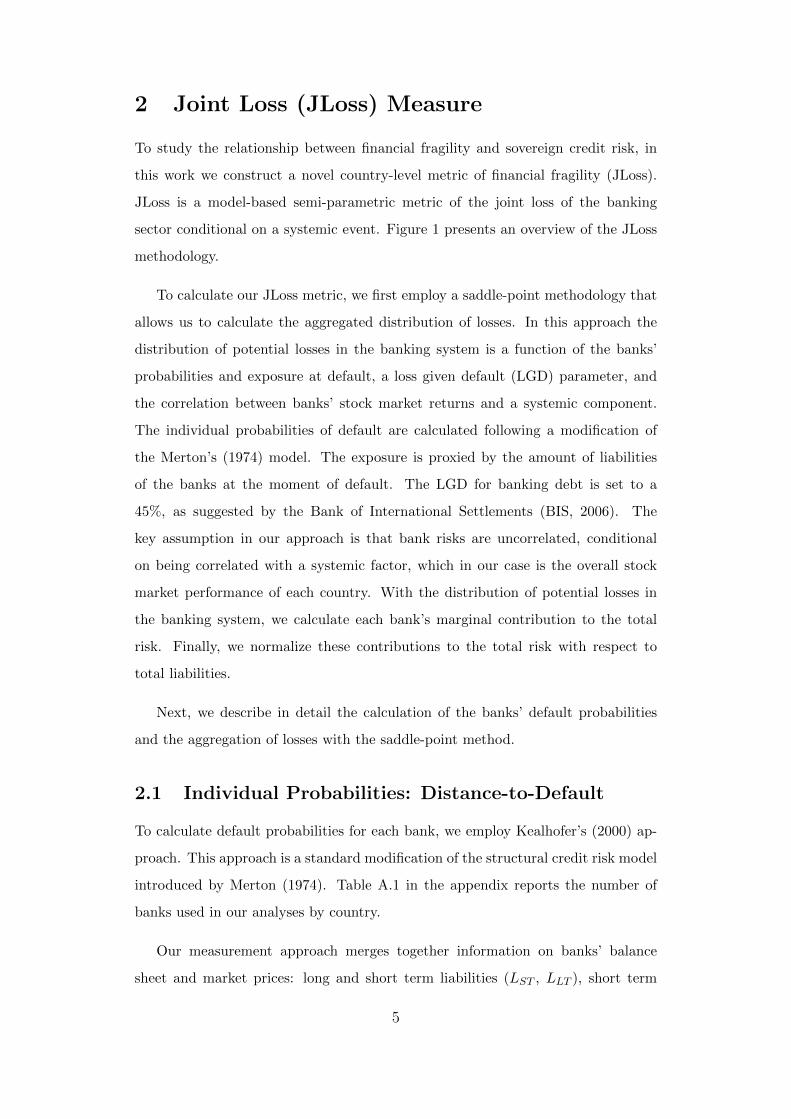
assets (AST ), average interest rates (r), time horizon (T ), volatility of bank real-

ized returns (σV ), and market capitalization (E). With this data we construct the

default point (D∗), which we formally define as

D∗ = LST +1

2LLT .

Then we numerically solve the following system of two non-linear equations, by

using the Newton-Raphson algorithm (Press et al., 2007), to project banks’ value

of assets (V ) and implied asset volatility (σA):

V

EΦ (d1)−

e−rTΦ (d2)

E/D∗− 1 = 0

Φ (d1)V

EσA − σE = 0.

Where d1 = log(V ED∗

)+

12σ2ET

σE√T

and d2 = d1 − σE√T . Φ stands for the cumulative

normal distribution function. 1

Once we get the projected values V and σA, we insert them into the following

distance to default DD equation:

DD =VE −D

∗

VE σA

.

This equation is a function of the predicted value of the banks’ assets (V ) and

asset volatility (σA). Finally, we assume normality to obtain the expected default

frequency (EDF ) as

EDF = Φ (−DD) .

We compute this quantity for all banks in every country and time periods of

our sample, and associate the expected default frequency value to the unconditional

probability of default (pdefi), which is one of the inputs for the saddle-point method.

1We use the realized variance approach to estimate the quarterly equity volatility. Following Barndorf-Nielsen et al. (2002), we compute square root of the sum of squared daily equity returns over a quarter.

That is, for every quarter and bank, we calculate σE =√∑Q

t=1 r2t , where Q is the number of days in a

particular quarter.

6

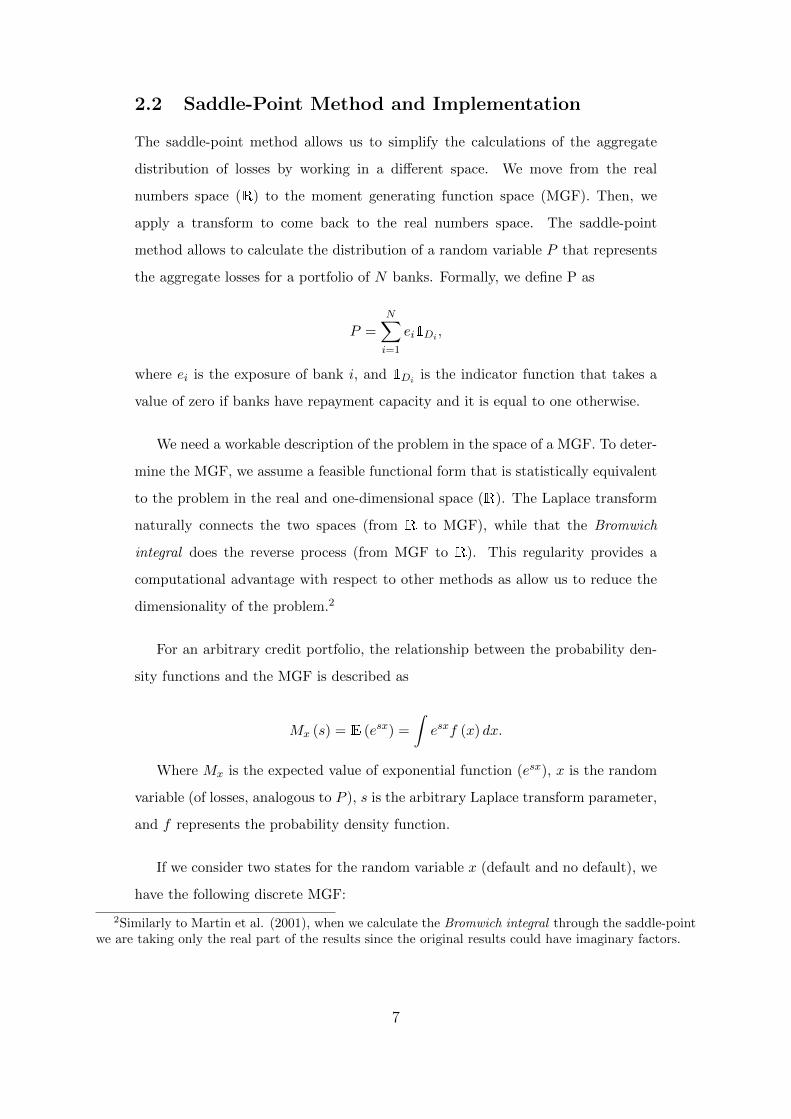
2.2 Saddle-Point Method and Implementation

The saddle-point method allows us to simplify the calculations of the aggregate

distribution of losses by working in a different space. We move from the real

numbers space (R) to the moment generating function space (MGF). Then, we

apply a transform to come back to the real numbers space. The saddle-point

method allows to calculate the distribution of a random variable P that represents

the aggregate losses for a portfolio of N banks. Formally, we define P as

P =N∑i=1

ei1Di ,

where ei is the exposure of bank i, and 1Di is the indicator function that takes a

value of zero if banks have repayment capacity and it is equal to one otherwise.

We need a workable description of the problem in the space of a MGF. To deter-

mine the MGF, we assume a feasible functional form that is statistically equivalent

to the problem in the real and one-dimensional space (R). The Laplace transform

naturally connects the two spaces (from R to MGF), while that the Bromwich

integral does the reverse process (from MGF to R). This regularity provides a

computational advantage with respect to other methods as allow us to reduce the

dimensionality of the problem.2

For an arbitrary credit portfolio, the relationship between the probability den-

sity functions and the MGF is described as

Mx (s) = E (esx) =

∫esxf (x) dx.

Where Mx is the expected value of exponential function (esx), x is the random

variable (of losses, analogous to P ), s is the arbitrary Laplace transform parameter,

and f represents the probability density function.

If we consider two states for the random variable x (default and no default), we

have the following discrete MGF:

2Similarly to Martin et al. (2001), when we calculate the Bromwich integral through the saddle-pointwe are taking only the real part of the results since the original results could have imaginary factors.

7

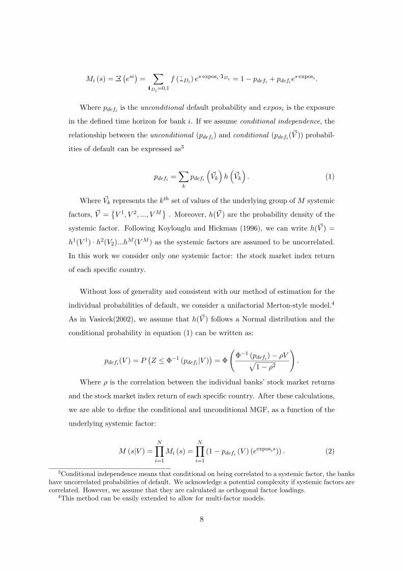
Mi (s) = E(esi)

=∑

1Di=0,1

f (1Di) es·exposi·1Di = 1− pdefi + pdefie

s·exposi .

Where pdefi is the unconditional default probability and exposi is the exposure

in the defined time horizon for bank i. If we assume conditional independence, the

relationship between the unconditional (pdefi) and conditional (pdefi(~V )) probabil-

ities of default can be expressed as3

pdefi =∑k

pdefi

(~Vk

)h(~Vk

). (1)

Where ~Vk represents the kth set of values of the underlying group of M systemic

factors, ~V ={V 1, V 2, ..., VM

}. Moreover, h(~V ) are the probability density of the

systemic factor. Following Koylouglu and Hickman (1996), we can write h(~V ) =

h1(V 1) · h2(V2)...hM (VM ) as the systemic factors are assumed to be uncorrelated.

In this work we consider only one systemic factor: the stock market index return

of each specific country.

Without loss of generality and consistent with our method of estimation for the

individual probabilities of default, we consider a unifactorial Merton-style model.4

As in Vasicek(2002), we assume that h(~V ) follows a Normal distribution and the

conditional probability in equation (1) can be written as:

pdefi(V ) = P(Z ≤ Φ−1 (pdefi |V )

)= Φ

(Φ−1 (pdefi)− ρV√

1− ρ2

).

Where ρ is the correlation between the individual banks’ stock market returns

and the stock market index return of each specific country. After these calculations,

we are able to define the conditional and unconditional MGF, as a function of the

underlying systemic factor:

M (s|V ) =

N∏i=1

Mi (s) =

N∏i=1

(1− pdefi (V ) (eexposis)) . (2)

3Conditional independence means that conditional on being correlated to a systemic factor, the bankshave uncorrelated probabilities of default. We acknowledge a potential complexity if systemic factors arecorrelated. However, we assume that they are calculated as orthogonal factor loadings.

4This method can be easily extended to allow for multi-factor models.

8

In order to further simplify the calculations, we use the cumulant generating

functions (K), defined as the logarithm of the MGF. Thus, K (s|V ) = log (M (s|V )).

The useful property of this function is that all moments of the distribution described

by the probability density f(·) can be generated by calculating the derivatives

evaluated at s = 0. For instance, for the two first moments we have K ′ (s = 0) =

E (x) and K ′′ (s = 0) = Var (x).

Once processed the information for the individual banks, the calculations per-

formed, and estimated the correlation structure, we are able to obtain the MGF

in equation (2). Next, we reverse the process to come back to the space of real

numbers and get the joint probability density of losses. To do that we employ the

Bromwich integral. Under our conditional independence assumption, this integral

takes the form:

f(x) =1

2πi

∫ +∞

−∞

(∫ +i∞

−i∞eK(s|V )−sxds

)h (V ) dV.

To solve the above integral, we use a particular property. Close to the saddle-

point of the argument of the exponential function, the integral can be approximated

with high level of accuracy. If we obtain the first order conditions for the argument

of the exponential, we obtain that dds (K (s)− sx), and K ′

(s = tV

)= x. In the

previous expression, t is the saddle point of the integral.

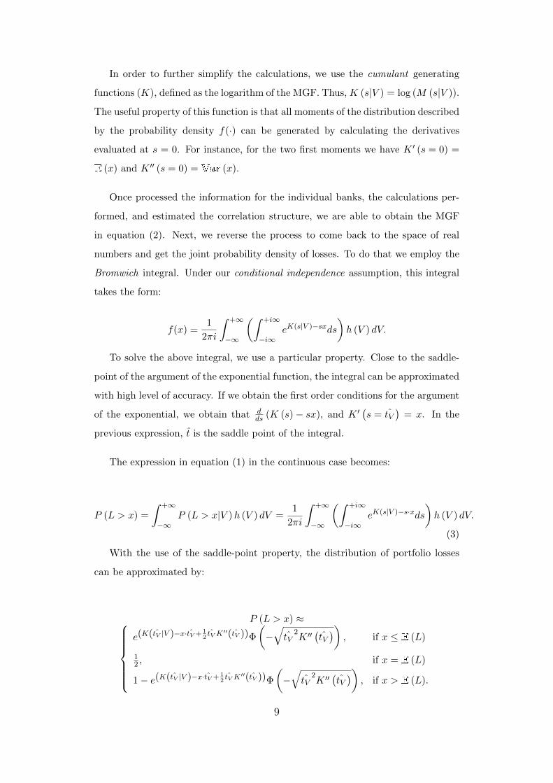
The expression in equation (1) in the continuous case becomes:

P (L > x) =

∫ +∞

−∞P (L > x|V )h (V ) dV =

1

2πi

∫ +∞

−∞

(∫ +i∞

−i∞eK(s|V )−s·xds

)h (V ) dV.

(3)

With the use of the saddle-point property, the distribution of portfolio losses

can be approximated by:

P (L > x) ≈e(K( ˆtV |V )−x· ˆtV + 1

2ˆtVK′′( ˆtV ))Φ

(−√tV

2K ′′(tV))

, if x ≤ E (L)

12 , if x = E (L)

1− e(K( ˆtV |V )−x· ˆtV + 12ˆtVK′′( ˆtV ))Φ

(−√tV

2K ′′(tV))

, if x > E (L).

9

In order to be able to manage the integral approximation, we need to discretize

the expression in (3). For the general case, in a multi-factor setting, we would have:

P (L > x) ≈∑k1

...∑kM

P(L > x|~V = {Vk1 , ..., VkM }

)h (Vk1) ...h (VkM ) (4)

Recall that in our case M , the number of systemic factors, is set to one. We

solve the expression in (4) by using a Gauss-Hermite quadrature. By applying the

Bayes theorem in (4), we get:

P (L > x) ≈∑j

P (j)P (L > x|j)h (Vk1) ...h (VkM ) . (5)

Where j is the state of the underlying systemic factor, thus P (L > x|j) is the

probability that the losses are greater than x for the systemic factor configuration

V . P (j) is the probability that the economy latent variable V is in the state j and it

corresponds to the quadrature weight hki . The marginal contributions to the overall

risk, from a particular bank to the entire financial system of a country, are obtained

following Martin (2001). Finally, to obtain our JLoss metric, we normalized with

respect to the total liabilities.

2.3 Parameterization

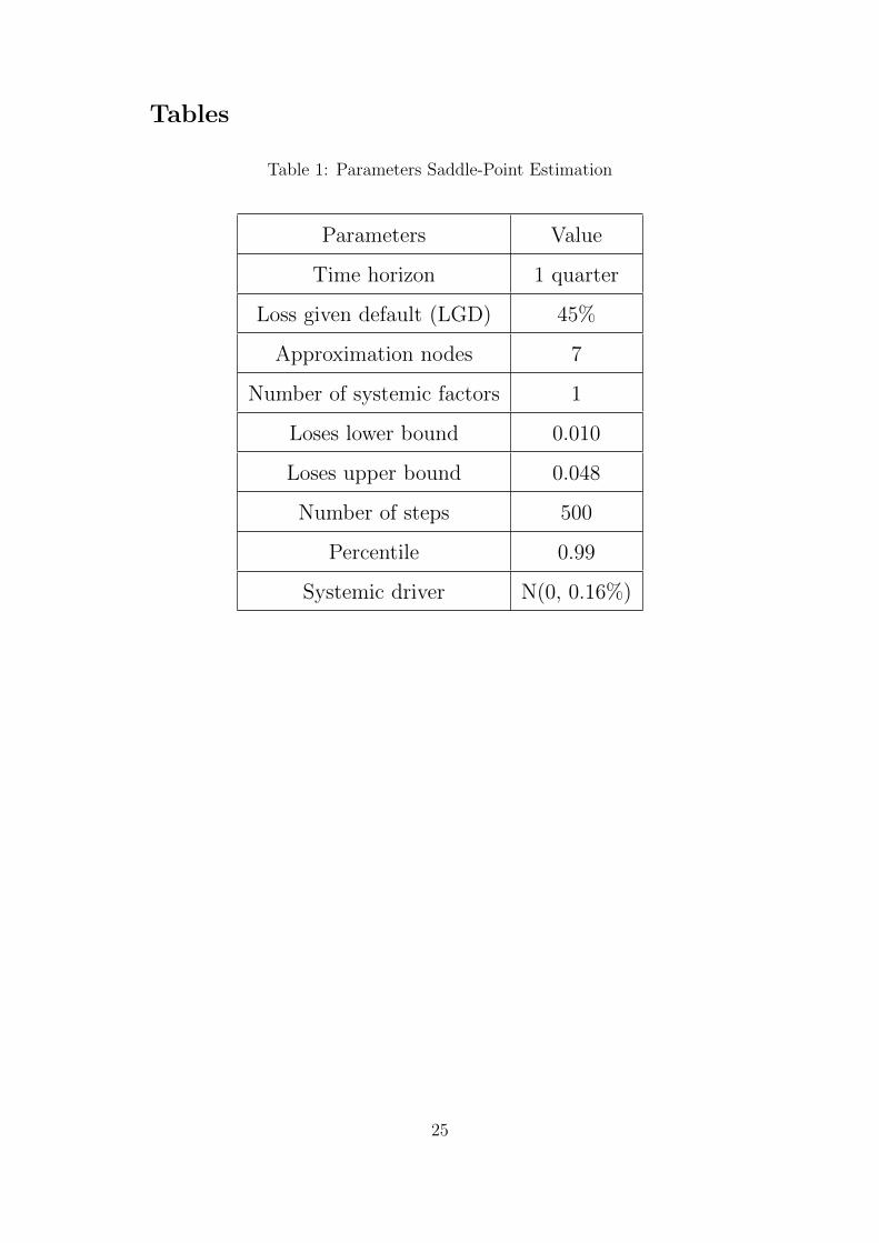
Table 1 shows the parameterization used in the Jloss calculation, once the individual

expected default frequencies are calculated. These parameters define the charac-

teristics of the aggregate distribution of losses and the method implemented. Time

span is quarterly, we use one systematic factor, and seven nodes for the integral

quadrature approximation.5 The lower bound of losses is fixed at 1 percent, whereas

the upper bound is assumed to be 4,8 percent. These values are calibrated to losses

in the emerging countries’ banking systems. Precision parameter is the 99 percent.

5The Gauss-Hermite quadrature solves integrals of the form I = 12π

∫ + inf

− infe−

x2

2 f(x)dx, as the sum

I =∑ni=1 wi · f(xi). In our case we are using n = 7. Therefore, we need to compute 7 saddle points. In

the standard numeric calculus literature, the quadrature is already tabulated to a generic integral. Wehave just to adjust it to our particular problem.

10

Finally, the systematic factor is assumed to have a normal distribution with zero

mean and variations between -4 and 4 percent. Table A.2 in Appendix A presents

the description and sources of all the variables used in the JLoss computation.

2.4 Discussion

A standard way of calculating the credit risk losses is the methodology described

in Vasicek (1997). However, this procedure has some shortcomings that can be

improved. The calculations require a functional form of the distribution of losses.

This assumption is strong because the estimated parameters of the distribution can

lead to important errors in the calculation of losses. Moreover, by being a method

that works in the space of real numbers, it lacks of a simple mathematical treatment

that allows closed form calculations. The semi-parametric saddle-point approach

used in this work, which heavily relies on Martin et al. (2001), has three main

advantages. First, it allows simple calculations because it has the ability to provide

statistical measures associated directly with credit risk. Second, it significantly

increases the speed of calculation in the computational implementation as it can be

presented in analytical formulas. Therefore, it allow us to construct our measure

for a long number of countries. Third, this method makes it possible to reduce a

n-dimensional problem to a single value.

Although Jloss is not the only attempt in the literature to measure financial

stability, it is one of the few that performs an aggregation work that allows us to

have a metric that reflects financial stability at the country level. For example, the

SRISK metric introduced by Brownless and Engle (2016) is an index that computes

the expected deficit to the capital of individual financial firms. Brownless and

Engle’s (2016) aggregation procedure consists of adding up all the capital losses

of a particular financial system. Thus, the aggregate metric does not consider the

correlation between the financial institutions. In addition, because the SRISK is a

metric based on capital deficits, given a particular stressed scenario, the metric is

more crisis oriented than identifying periods of vulnerability.

The CIMDO-copula introduced by Segoviano (2009) is a metric more similar

to the JLoss in methodological terms. However, the difference between the JLoss

and the Segoviano CIMDO-copula is that in the first case, the assumptions of

11

conditional independence and the semi-parametric calculation allow us to improve

efficiency in capturing the changes of variation and offer advantages from the com-

putational point of view, being an approximation but with high precision.

3 Data

To empirically test the relationship between sovereign credit risk, financial fragility,

and global factors, we employ a quarterly panel dataset of 19 emerging economies

over the period 1999:Q1 to 2017:Q3. Our panel dataset contains variables related

to sovereign credit risk, financial fragility in the banking sector, country-specific

macroeconomic conditions, and global financial factors. The countries in our anal-

ysis are those classified as emerging markets in the J. P. Morgan Emerging Markets

Bonds Index (EMBI Global) and those for which we had data to construct the JLoss

metric during our sample period. The countries in our sample are: Argentina,

Brazil, Bulgaria, Chile, China, Colombia, Egypt, Indonesia, Malaysia, Mexico,

Pakistan, Panama, Peru, Poland, Philippines, Russia, South Africa, Turkey, and

Venezuela.

Table A.2 in Appendix A presents the description and sources of all the variables

used in our regression analysis. Our final sample consists of 1,187 country-time

observations in the spreads regressions and 1,243 country-time observations in the

rating regressions. Table 2 reports summary statistics of all the variables used in

the regression analysis for the overall sample.

3.1 Sovereign Credit Risk

The sovereign-credit-risk measures used in this study are the sovereign bond spread

and the sovereign credit rating. These variables are obtained from the Bloomberg

system that collects data from industry sources. Emerging-market sovereign bond

spreads are measured using the EMBI Global, which measures the average spread

on U.S. dollar-denominated bonds issued by sovereign entities over U.S. Treasuries.

It reflects investors’ perception of a government’s credit risk. Our sovereign-credit-

rating variable is constructed based on Standard & Poor’s (S&P) ratings for long-

12

term debt in a foreign currency.6 To compute a quantitative measure of sovereign

credit ratings, we follow the existing literature and map the credit-rating categories

into 21 numerical values (see, e.g., Borensztein et al., 2013), with a value of 21 cor-

responding to the highest rating (AAA) and 1 to the lowest (SD/D). For robustness

purposes, we also consider Moody’s sovereign credit ratings for long-term debt in

foreign currency. Table A.3 in the appendix reports the numerical values for each

credit-rating category.

Tables 3 and 4 provide summary information for the sovereign credit spreads

and sovereign credit ratings by country, respectively. The average values of the

spreads range widely across countries. The lowest average is 125 basis points for

China; the highest average is 1,395 basis points for Argentina. Both the standard

deviations and the minimum/maximum values indicate significant variations also

exist over time. For example, the credit spread for Argentina ranges from 204 to

7,078 basis points during the sample period. The average values of the ratings

also range widely across countries. The lowest average rating is 6.5 for Argentina;

the highest average is 13.2 for Poland. Again, the descriptive statistics indicate

significant variations over time. For instance, the credit rating for Russia ranges

from 1 to 14 during the sample period.

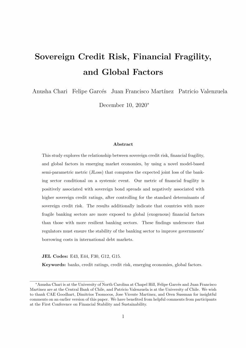
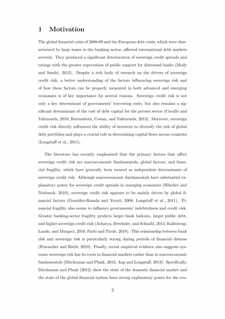
3.2 Domestic Financial Fragility

Our key explanatory variable of interest is our metric of financial fragility (JLoss).

JLoss is calculated using stock market and balance-sheet data of commercial banks

that are listed in the stock market of the 19 emerging economies in our sample.

Table A.1 in the appendix reports the number of banks by each country. Figure 1

displays the JLoss metric for each of the 19 emerging countries in the sample.

As shown in Figure 1, in most countries our JLoss metric captures both periods

6Standard and Poor’s (2001) defines a foreign-currency credit rating as “A current opinion of anobligor’s overall capacity to meet its foreign-currency-denominated financial obligations. It may takethe form of either an issuer or an issue credit rating. As in the case of local currency credit ratings, aforeign currency credit opinion on Standard and Poor’s global scale is based on the obligor’s individualcredit characteristics, including the influence of country or economic risk factors. However, unlike localcurrency ratings, a foreign currency credit rating includes transfer and other risks related to sovereignactions that may directly affect access to the foreign exchange needed for timely servicing of the ratedobligation. Transfer and other direct sovereign risks addressed in such ratings include the likelihood offoreign exchange control and the imposition of other restrictions on the repayment of foreign debt.”

13

of global financial distress and periods of country-specific idiosyncratic financial

fragility. In many countries, idiosyncratic factors seems to have stronger effects

on financial fragility than global factors. For example, for the case of Argentina

our metric shows that the fragility generated by the sub-prime crisis was smaller

than the fragility generated by the 2001 Argentinean sovereign default. In Brazil,

idiosyncratic factors such as the ”Impeachment” of Dilma Rousseff also seem to

have a much stronger effect on financial fragility than global financial fragility.

3.3 Global Factors

Far from being autarkies, the emerging economies included in this paper have in-

creasingly become more financially integrated with the rest of the world. Therefore,

their ability and willingness to serve their debt may depend not only on macroeco-

nomic domestic conditions, but also on the state of the global economy. To capture

broad changes in the state of the global (exogenous) financial markets, we consider

a set of global financial factors that reflect financial market volatility, risk-free in-

terest rates, risk premiums, and market illiquidity. Specifically, the global financial

factors used in this study are the CBOE Volatility Index, the 10-year U.S. Trea-

sury rate, the 10-year U.S. High Yield spread, and the On/off-the-run U.S. Treasury

spread. For robustness, we also employ the noise measure as an additional measure

of market illiquidity.

The CBOE Volatility Index, known commonly as the VIX, measures the mar-

ket’s expectation for 30-day volatility in the S&P 500. Usually, a higher VIX

indicates a general increase in the risk premium and, consequently, an increase in

the cost of financing for emerging economies. The 10-year U.S. Treasury rate ad-

dresses the interest rate effect. It reflects the risk-free rate against which investors

in advanced economies evaluate the payoffs of all other assets of similar maturities.

The high-yield spread proxies for the price of risk in the global financial market.

We employ J. P. Morgan’s High Yield Spread Index, which measures the spread

over the U.S. Treasuries yield curve. The On/off-the-run U.S. Treasury spread is

the spread between the yield of on-the-run and off-the-run U.S. Treasury bonds.

Although the issuer of both types of bonds is the same, on-the-run bonds generally

trade at a higher price than similar off-the-run bonds, because of the greater liq-

14

uidity and specialness of on-the-run bonds in the repo markets.7 We compute the

On/off-the-run U.S. Treasury spread using 10-year bonds, given that the spread

tends to be small and noisy at smaller maturities. The data sources used in the

construction of this spread are from Gurkaynak et al. (2007) and the Board of

Governors of the Federal Reserve System. Lastly, the noise measure captures the

amount of aggregate illiquidity in the U.S. bond market (Hu, Pan, and Wang, 2013).

It is the aggregation of the price deviations across U.S. Treasury bonds. The pri-

mary concept behind this measure is that the lack of arbitrage capital reduces the

power of arbitrage and that assets can be traded at prices that deviate from their

fundamental values.

3.4 Country-Specific Factors

To capture the domestic macro environment, we also control for a set of time-varying

country-level macro variables that may directly affect sovereign credit risk: debt to

GDP, exchange-rate volatility, profit margin in the banking sector, and GDP per

capita. In the spread regressions, we also control for the long-term foreign-currency

sovereign credit rating. The debt-to-GDP ratio captures the degree of the economy

indebtedness. Exchange-rate volatility is the volatility of the country’s exchange

rate against the U.S. dollar. We added this variable because it is considered a

major determinant of firms’ revenues from abroad and their ability to repay debts

denominated in dollars. Profit margin in the banking sector captures the degree

of competitiveness in the domestic financial sector. Sovereign credit ratings are

credit-rating agencies’ opinion of a government’s overall capacity to meet its foreign-

currency-denominated financial obligations. Finally, for robustness purposes, we

also control in a set of regressions for periods of domestic systemic banking crises

(Laeven and Valencia, 2018).

7This specialness arises from the fact that on-the-run Treasury bond holders are frequently able topledge these bonds as collateral and borrow in the repo market at considerably lower interest rates thanthose of similar loans collateralized by off-the-run Treasury bonds (Sundaresan and Wang, 2009).

15

4 Regression Analysis and Results

The first objective of this study is to explore the relationship between sovereign

credit risk and financial fragility, controlling for other factors that might affect

sovereign credit risk independently. We estimate the following baseline econometric

model:

Credit Riskc,t = αc + γt + βJLossc,t + ωXc,t + εc,t, (6)

where Credit Riskc,t is either the sovereign credit spread or the sovereign credit rat-

ing of country c at time t. JLossc,t is our metric of financial fragility in the banking

sector that computes the joint loss distribution of the banking sector conditional

on a systemic event. Both Credit Riskc,t and JLossc,t are expressed in natural

logarithm. Xc,t is a set of time-varying country-level macro variables, including the

sovereign credit rating in the spread regressions. The term αc represents a vector

of country fixed effects that control for all time-invariant country-specific factors

affecting both credit risk and financial fragility. The term γt captures time fixed

effects that control for common and global shocks affecting all countries, such as

global financial crises or changes in the world business cycle. εc,t is the error term.

Our specification including country fixed effects and time fixed effects is anal-

ogous to a difference-in-differences estimator in a multiple-treatment-group and

multiple-time-period setting (Imbens and Wooldridge, 2009). The identification

assumption is that in the absence of domestic financial fragility, the sovereign bond

spreads and sovereign credit ratings are exposed to similar global shocks. We be-

lieve this assumption is plausible, given the homogeneous nature of our sample

(i.e., emerging economies that issue international bonds denominated in U.S. dol-

lars) and that global factors are crucial determinants of sovereign credit risk in

emerging economies (Gonzalez-Rosada and Yeyati, 2008).

The second objective of this study is to examine whether the effect of global (ex-

ogenous) financial factors on sovereign credit risk is stronger in countries with more

vulnerable banking sectors. To explore this hypothesis, we estimate the following

model:

16

Credit Riskc,t = αc + γt + βJLossc,t + θJLossc,t x Globalt + ωXc,t + εc,t, (7)

where Globalt is a global (exogenous) financial factor at time t. The coefficient

associated with the interaction term, JLossc,t x Globalt, captures whether the

impact of global financial factors on sovereign credit risk differs in countries with

different degrees of financial fragility in their banking sectors. We hypothesize that

in a financially integrated world where domestic banks and international capital

markets work as substitute sources of capital, a stronger banking sector should

attenuate a country’s exposure to global financial factors.

4.1 Sovereign Bond Spreads and Financial Fragility

Table 5 presents the results from the estimation of equation (1) by using sovereign

credit spreads as our dependent variable. The model is estimated by ordinary least

squares (OLS) with robust standard errors. The table also reports the estimates

of our econometric model by directly including global financial factors instead of

time fixed effects. The results suggest sovereign credit spreads are positively related

to our metric of banking fragility (JLoss). This positive correlation between JLoss

and sovereign credit spreads is statistically significant and economically meaningful,

even after controlling for country and time fixed effects (column 1), for sovereign

credit ratings (column 2), and for the standard determinants of sovereign credit

risk (column 3). We also find similar results when we control for a number of

global financial factors instead of time fixed effects (column 4). Given that both

the spread and the JLoss metric are expressed in natural logarithm, our estimated

coefficients represent an elasticity. Our regressions appear to support the view

that banking fragility exerts a strong influence on the pricing of emerging-market

sovereign bonds.

Most of the estimated coefficients of our control variables are statistically signif-

icant in the expected direction. The results show, on the one hand, that sovereign

credit ratings are negatively related to credit spreads. On the other hand, the re-

sults show indebtedness, global financial instability, global premiums, and aggregate

17

market liquidity are positively related to sovereign credit spreads.

4.2 Sovereign Credit Ratings and Financial Fragility

Our previous analysis indicates sovereign credit spreads are larger during periods

of fragility in the banking sector, even after controlling for credit ratings and other

standard determinants of sovereign credit risk. However, credit spreads and finan-

cial fragility could also be linked through a credit-rating channel. Whereas credit

spreads are a direct indicator of the effective cost of debt capital, credit ratings

are rating agencies’ opinions about debt issuers’ probability of default. Given that

these ratings consider business and financial risk factors, they are likely to capture

some components associated with financial fragility.

To explore a potential credit-rating channel, Table 6 reports the results from our

baseline model by using sovereign credit ratings as our dependent variable. Columns

1 and 2 report the results of our model with country fixed effects and time fixed

effects, and column 3 reports the results of our model including global financial

factors instead of time fixed effects. Overall, our results indicate sovereign credit

ratings are negatively related to our JLoss metric. Remember that this negative

correlation between JLoss and sovereign credit ratings is statistically significant and

economically meaningful in all our specifications.

Overall, our results suggest both the market and the credit-rating agencies con-

sider the fragility of the banking sector a crucial determinant of sovereign credit

risk in emerging markets.

4.3 Are Countries with Fragile Banking Sectors More

Exposed to Global Financial Shocks?

Although the literature has explored the relevance of external factors as significant

determinants of sovereign credit risk in emerging economies (see, e.g., Gonzalez-

Rosada and Yeyati, 2008), little research has explored the aspects that make a

country more or less resilient to sudden changes in the external context. We ex-

plore whether global financial factors affect sovereigns differently depending on the

fragility of their banking sectors. Given that the emerging economies included in

18

this paper have increasingly become more financially integrated with the rest of the

world and that domestic and international capital markets can provide an alterna-

tive source of funding that can complement bank financing, we hypothesize that

global financial conditions should typically have a smaller effect on countries with

more resilient banking sectors.

Tables 7 and 8 report the results from the estimation of equation (2) by using

sovereign credit spreads and sovereign credit ratings as our dependent variables,

respectively. As before, the model is estimated by ordinary least squares (OLS)

with robust standard errors. The tables also report the estimates of our econometric

model including global financial factors instead of time fixed effects (columns 5

to 8). The positive and statistically significant coefficients associated with the

interaction terms in columns 1 to 4 in Table 7 indicate that a deterioration in

global market volatility, risk-free interest rates, high-yield spreads, and aggregate

illiquidity produce a higher increase in sovereign credit spreads of countries with

more fragile banking sectors. These effects are highly statistically significant and

economically meaningful. Columns 5 to 8 in Table 7, which consider the direct

effects of global financial factors instead of time fixed effects, show almost identical

results.

Similar to our previous results, the negative and statistically significant coeffi-

cients associated with the interaction terms in columns 1 to 4 in Table 8 indicate

that deterioration in global financial market volatility, risk-free interest rates, high-

yield spreads, and aggregate illiquidity produced a higher deterioration in sovereign

credit ratings of countries with more fragile banking sectors. Columns 5 to 8 in the

table report qualitatively similar results.

5 Robustness Checks

We conduct a number of exercises to check the robustness of our main results. First,

we control for periods of systemic banking crises. Then, we exclude banking crisis

periods of our sample. Next, we explore whether our interaction term is capturing

another non-linear effect of global factors on sovereign credit spreads. Finally, we

consider Moody’s sovereign credit ratings instead of S&P ratings.

19

Given that our metric of financial fragility in the banking sector spikes during

periods of systemic banking crises, our results are likely driven by a few observations

that capture a very high correlation between sovereign risk and banking risk during

periods of financial turmoil. Columns 1 and 2 of Table 9 report the results from

estimating our baseline regressions controlling for dummy variables associated with

periods of systemic banking crises, and columns 3 and 4 report the results when

excluding periods of systemic banking crises. The systemic-banking-crises dummy

variables used in our analysis were constructed using the dataset introduced by

Laeven and Valencia (2018). The results are qualitatively identical to our base-

line regressions reported in Tables 5 and 6. As expected, the magnitude of our

coefficients decrease. However, they remain highly statistically significant in the

expected directions.

Because our primary term of interest in Table 7 is the interaction between JLoss

and our four global factors, JLoss may captures the effect of another country-specific

factor. Table 10 presents the results of a more explicit test of this possibility by

including a number of additional interaction terms. The added terms correspond

to the interaction of the sovereign credit rating and the banking-crisis dummy

variable with our four different measures associated with global factors, respectively.

Columns 1 to 4 augment our previous model with the interaction between global

factors and sovereign credit ratings, and columns 5 to 8 augment our previous model

with the interaction between global factors and banking crises. Overall, our main

findings remain unchanged.

Finally, we find in unreported regressions that an alternative measure of the

sovereign credit rating constructed based on the ratings granted by Moody’s yields

results almost identical to all those results obtained using S&P sovereign credit

ratings.

6 Conclusion

The global financial crisis of 2008-09 and the European debt crisis generated large

losses in the banking sector, triggering a significant deterioration of sovereign credit

risk with the greater expectation of public support for distressed banks. These

20

events spurred a renewed interest in generating new measures of financial fragility

as well as in understanding the consequences of such vulnerabilities. Despite a new

large body of research on the relationship between sovereign risk and bank risk in

the eurozone, rigorous research on the nexus between sovereign risk and bank risk

in emerging markets is scant. A better understanding of the factors influencing

sovereign risk and of how these factors can be properly measured in both advanced

and emerging economies is of key importance.

The goal of this paper is to shed light on the relationship between sovereign

credit risk and financial fragility in the banking sector. To achieve this goal, we

develop a novel model-based semi-parametric metric (JLoss) that computes the

joint-loss distribution of a country’s banking sector conditional on a systemic event.

We find that, controlling for country-level macro variables as well as for country and

time fixed effects, our metric of financial fragility (JLoss) is positively associated

with sovereign credit spreads and negatively associated with higher sovereign credit

ratings in our sample of emerging economies.

We also explore whether bank stability reduce a country’s exposure to global

financial factors. A better understanding of the mechanisms through which global

factors influence sovereign credit risk is crucial. As highlighted by Gonzalez-Rosada

and Yeyati (2008), emerging economies need to formulate mechanisms to reduce

their exposure to global financial factors, as the process of financial integration

exhibited over the past four decades brings contagion from other advanced and

emerging economies. Our results indicate that countries with more fragile banking

sectors are more exposed to the influence of global financial factors.

Our results have important policy implications because they underscore that

the stability of a country’s domestic banking sector plays a crucial role in reduc-

ing sovereign risk and its sensitivity to global factors. Therefore, countries must

implement policies oriented to improve the stability of their banking sectors to im-

prove their access to international capital and reduce potentially undesired effects

of integration.

21

References

[1] Acharya, V., and Naqvi, H. The seeds of a crisis: A theory of bank liquidity

and risk taking over the business cycle. Journal of Financial Economics 106,

2 (2012), 349–366.

[2] Ang, A., and Longstaff, F. A. Systemic sovereign credit risk: Lessons

from the us and europe. Comision Presidencial de Isapres 60, 5 (2013), 493–

510.

[3] Barndorff-Nielsen, O., N. E., and Shepard, N. Some recent develop-

ments in stochastic volatility modelling. Journal Quantitative Finance 2, 1

(2002), 11–23.

[4] Boehmer, E., and Megginson, W. L. Determinants of secondary market

prices for developing country syndicated loans. The Journal of Finance 45, 5

(1990), 1517–1540.

[5] Borensztein, E., Cowan. K., and Valenzuela, P. Sovereign ceilings

“lite”?: The impact of sovereign ratings on corporate ratings. Journal of

Banking and Finance 37, 11 (2013), 4014–4024.

[6] Brownlees, C., and Engle, R. F. Srisk: A conditional capital shortfall

measure of systemic risk. The Review of Financial Studies 30, 1 (2016), 48–79.

[7] Cavallo, E., and Valenzuela, P. The determinants of corporate risk in

emerging markets: an option-adjusted spread analysis. International Journal

of Finance and Economics 15, 1 (2010), 59–74.

[8] Dieckmann, S., and Plank, T. Default risk of advanced economies: An

empirical analysis of credit default swaps during the financial crisis. Review of

Finance 16, 4 (2012), 903–934.

[9] Edwards, S. The pricing of bonds and bank loans in international markets:

An empirical analysis of developing countries’ foreign borrowing. European

Economic Review 30, 3 (1986), 565–589.

[10] Farhi, E., and Tirole, J. Collective moral hazard, maturity mismatch, and

systemic bailouts. American Economic Review 102, 1 (2012), 60–93.

22

[11] Fratzscher, M., and Rieth, M. H. Monetary policy, bank bailouts and

the sovereign-bank risk nexus in the euro area. Review of Finance, 23 (2019),

745–775.

[12] Gonzalez-Rozada, M., and Yeyati, E. L. Global factors and emerging

market spreads. The Economic Journal 118, 533 (2008), 1917–1936.

[13] Gurkaynak, R. S., Sack. B., and Wright, J. H. The us treasury yield

curve: 1961 to the present. Journal of Monetary Economics 54, 8 (2007),

2291–2304.

[14] Hilscher, J., and Nosbusch, Y. Determinants of sovereign risk: Macroe-

conomic fundamentals and the pricing of sovereign debt. Review of Finance

14, 2 (2010), 235–262.

[15] Hu, G. X., Pan. J., and Wang, J. Noise as information for illiquidity. The

Journal of Finance 68, 6 (2013), 2341–2382.

[16] Imbens, G. W., and Wooldridge, J. M. Recent developments in the

econometrics of program evaluation. Journal of Economic Literature 47, 1

(2009), 5–86.

[17] Kallestrup, R., Lando. D., and Murgoci, A. Financial sector linkages

and the dynamics of bank and sovereign credit spreads. Journal of Empirical

Finance 38 (2016), 374–393.

[18] Kealhofer, S., and Kurbat, M. Benchmarking quantitative default risk

models: A validation methodology. Research Paper, Moody’s KMV (2000).

[19] Koylouglu, H., and Hickman, A. Reconcilable differences. Risk 11, 10

(1998), 56–62.

[20] Laeven, L., and Valencia, F. Systemic banking crises revisited. Working

Paper No. 18/206 (2018).

[21] Longstaff, F. A., Pan. J. Pedersen. L. H., and Singleton, K. J. How

sovereign is sovereign credit risk? American Economic Journal: Macroeco-

nomics 3, 2 (2011), 75–103.

[22] Martin, R., Thompson. K., and Browne, C. Taking to the saddle: An

analytical technique to construct the loss distribution of correlated events.

Risk-London-Risk Magazine Limited 14, 6 (2001), 91–94.

23

[23] Merton, R. C. On the pricing of corporate debt: The risk structure of

interest rates. The Journal of Finance 29, 2 (1974), 449–470.

[24] Mody, A., and Sandri, D. The eurozone crisis: How banks and sovereigns

came to be joined at the hip. Economic Policy 27, 70 (2012), 199–230.

[25] Press, W. H., Teukolsky. S. A. Vetterling. W. T., and Flannery,

B. P. Numerical Recipes 3rd Edition: The Art of Scientific Computing. Cam-

bridge University Press, 2007.

[26] Standard, and Poor’s. Rating methodology: Evaluating the issuer, 2001.

http://www.standardandpoors.com/.

[27] Sundaresan, S., and Wang, Z. Y2k and liquidity premium in treasury

bond markets. Review of Financial Studies 22, 3 (2009), 1021–1056.

[28] Vasicek, O. The loan loss distribution. KMV Corporation (1997).

24

Tables

Table 1: Parameters Saddle-Point Estimation

Parameters Value

Time horizon 1 quarter

Loss given default (LGD) 45%

Approximation nodes 7

Number of systemic factors 1

Loses lower bound 0.010

Loses upper bound 0.048

Number of steps 500

Percentile 0.99

Systemic driver N(0, 0.16%)

25

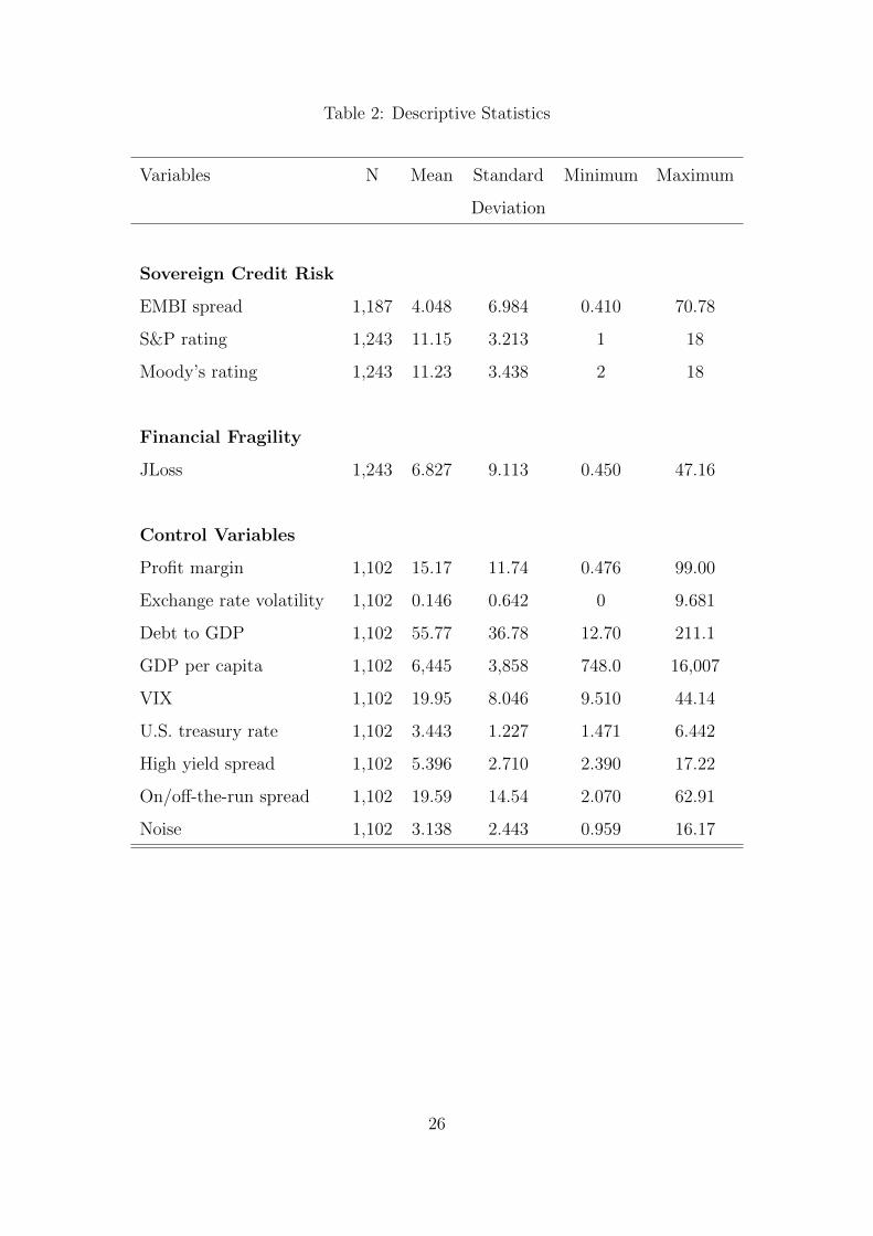
Table 2: Descriptive Statistics

Variables N Mean Standard Minimum Maximum

Deviation

Sovereign Credit Risk

EMBI spread 1,187 4.048 6.984 0.410 70.78

S&P rating 1,243 11.15 3.213 1 18

Moody’s rating 1,243 11.23 3.438 2 18

Financial Fragility

JLoss 1,243 6.827 9.113 0.450 47.16

Control Variables

Profit margin 1,102 15.17 11.74 0.476 99.00

Exchange rate volatility 1,102 0.146 0.642 0 9.681

Debt to GDP 1,102 55.77 36.78 12.70 211.1

GDP per capita 1,102 6,445 3,858 748.0 16,007

VIX 1,102 19.95 8.046 9.510 44.14

U.S. treasury rate 1,102 3.443 1.227 1.471 6.442

High yield spread 1,102 5.396 2.710 2.390 17.22

On/off-the-run spread 1,102 19.59 14.54 2.070 62.91

Noise 1,102 3.138 2.443 0.959 16.17

26

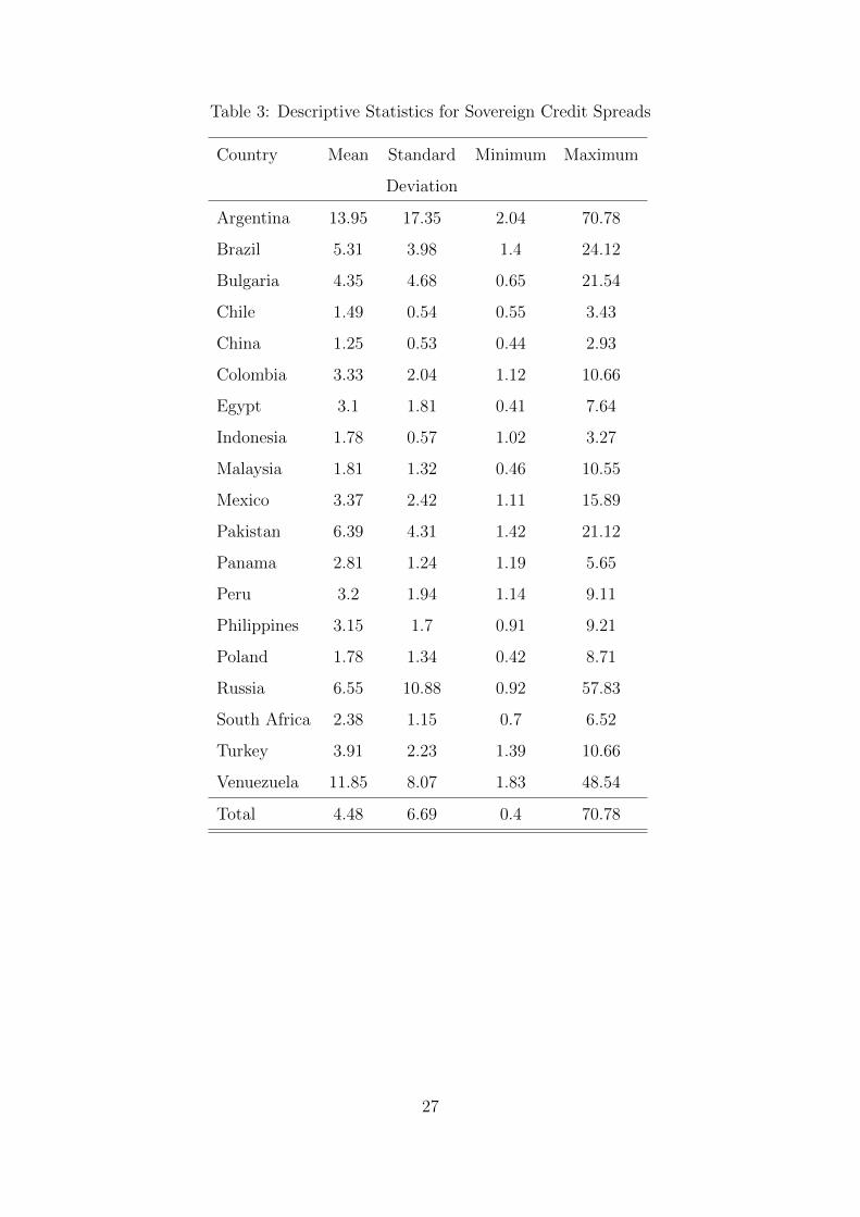
Table 3: Descriptive Statistics for Sovereign Credit Spreads

Country Mean Standard Minimum Maximum

Deviation

Argentina 13.95 17.35 2.04 70.78

Brazil 5.31 3.98 1.4 24.12

Bulgaria 4.35 4.68 0.65 21.54

Chile 1.49 0.54 0.55 3.43

China 1.25 0.53 0.44 2.93

Colombia 3.33 2.04 1.12 10.66

Egypt 3.1 1.81 0.41 7.64

Indonesia 1.78 0.57 1.02 3.27

Malaysia 1.81 1.32 0.46 10.55

Mexico 3.37 2.42 1.11 15.89

Pakistan 6.39 4.31 1.42 21.12

Panama 2.81 1.24 1.19 5.65

Peru 3.2 1.94 1.14 9.11

Philippines 3.15 1.7 0.91 9.21

Poland 1.78 1.34 0.42 8.71

Russia 6.55 10.88 0.92 57.83

South Africa 2.38 1.15 0.7 6.52

Turkey 3.91 2.23 1.39 10.66

Venuezuela 11.85 8.07 1.83 48.54

Total 4.48 6.69 0.4 70.78

27

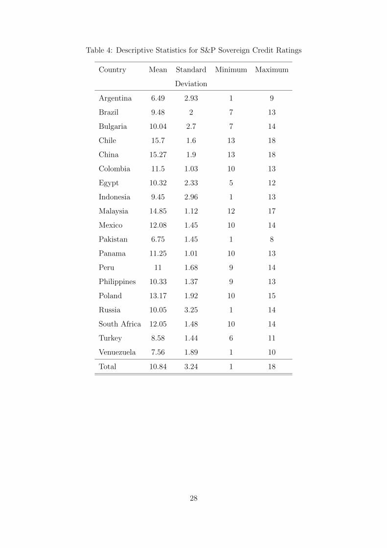
Table 4: Descriptive Statistics for S&P Sovereign Credit Ratings

Country Mean Standard Minimum Maximum

Deviation

Argentina 6.49 2.93 1 9

Brazil 9.48 2 7 13

Bulgaria 10.04 2.7 7 14

Chile 15.7 1.6 13 18

China 15.27 1.9 13 18

Colombia 11.5 1.03 10 13

Egypt 10.32 2.33 5 12

Indonesia 9.45 2.96 1 13

Malaysia 14.85 1.12 12 17

Mexico 12.08 1.45 10 14

Pakistan 6.75 1.45 1 8

Panama 11.25 1.01 10 13

Peru 11 1.68 9 14

Philippines 10.33 1.37 9 13

Poland 13.17 1.92 10 15

Russia 10.05 3.25 1 14

South Africa 12.05 1.48 10 14

Turkey 8.58 1.44 6 11

Venuezuela 7.56 1.89 1 10

Total 10.84 3.24 1 18

28

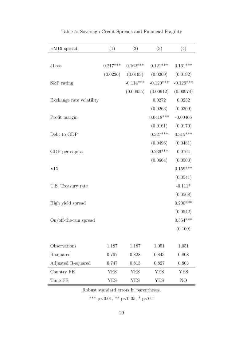
Table 5: Sovereign Credit Spreads and Financial Fragility

EMBI spread (1) (2) (3) (4)

JLoss 0.217*** 0.162*** 0.121*** 0.161***

(0.0226) (0.0193) (0.0209) (0.0192)

S&P rating -0.114*** -0.120*** -0.126***

(0.00955) (0.00912) (0.00974)

Exchange rate volatility 0.0272 0.0232

(0.0263) (0.0309)

Profit margin 0.0418*** -0.00466

(0.0161) (0.0170)

Debt to GDP 0.327*** 0.315***

(0.0496) (0.0481)

GDP per capita 0.239*** 0.0764

(0.0664) (0.0503)

VIX 0.159***

(0.0541)

U.S. Treasury rate -0.111*

(0.0568)

High yield spread 0.200***

(0.0542)

On/off-the-run spread 0.554***

(0.100)

Observations 1,187 1,187 1,051 1,051

R-squared 0.767 0.828 0.843 0.808

Adjusted R-squared 0.747 0.813 0.827 0.803

Country FE YES YES YES YES

Time FE YES YES YES NO

Robust standard errors in parentheses.

*** p<0.01, ** p<0.05, * p<0.1

29

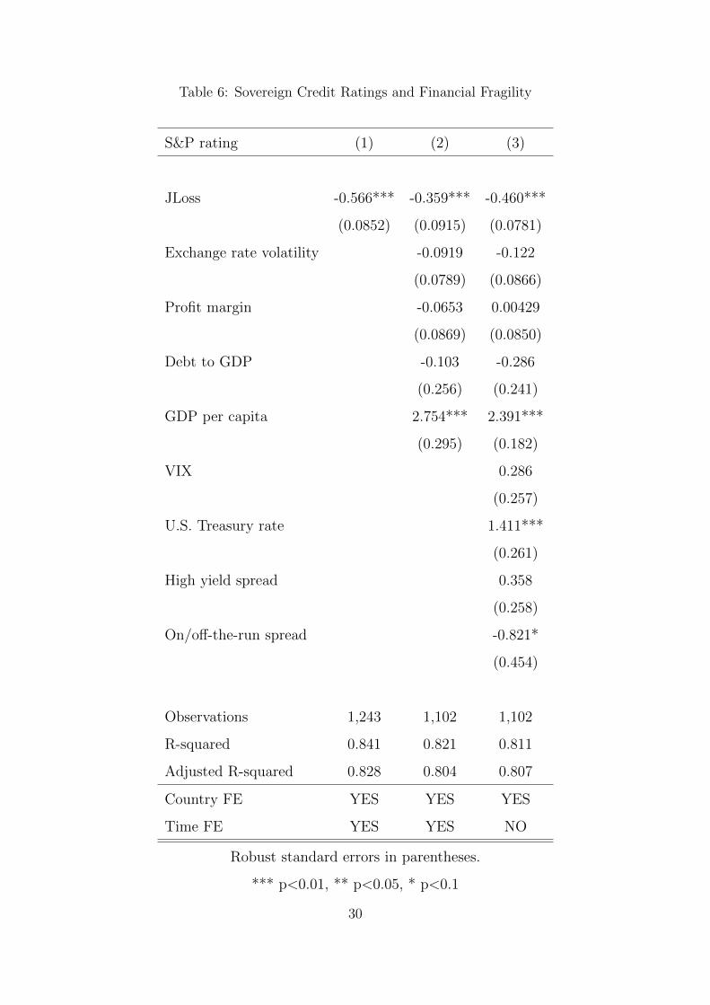
Table 6: Sovereign Credit Ratings and Financial Fragility

S&P rating (1) (2) (3)

JLoss -0.566*** -0.359*** -0.460***

(0.0852) (0.0915) (0.0781)

Exchange rate volatility -0.0919 -0.122

(0.0789) (0.0866)

Profit margin -0.0653 0.00429

(0.0869) (0.0850)

Debt to GDP -0.103 -0.286

(0.256) (0.241)

GDP per capita 2.754*** 2.391***

(0.295) (0.182)

VIX 0.286

(0.257)

U.S. Treasury rate 1.411***

(0.261)

High yield spread 0.358

(0.258)

On/off-the-run spread -0.821*

(0.454)

Observations 1,243 1,102 1,102

R-squared 0.841 0.821 0.811

Adjusted R-squared 0.828 0.804 0.807

Country FE YES YES YES

Time FE YES YES NO

Robust standard errors in parentheses.

*** p<0.01, ** p<0.05, * p<0.1

30

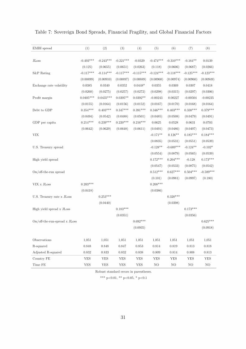
Table 7: Sovereign Bond Spreads, Financial Fragility, and Global Financial Factors

EMBI spread (1) (2) (3) (4) (5) (6) (7) (8)

JLoss -0.493*** -0.243*** -0.221*** -0.0329 -0.474*** -0.310*** -0.164** 0.0139

(0.125) (0.0655) (0.0651) (0.0263) (0.118) (0.0606) (0.0687) (0.0266)

S&P Rating -0.117*** -0.114*** -0.117*** -0.115*** -0.124*** -0.118*** -0.125*** -0.123***

(0.00899) (0.00910) (0.00897) (0.00889) (0.00960) (0.00974) (0.00960) (0.00949)

Exchange rate volatility 0.0385 0.0340 0.0352 0.0448* 0.0355 0.0369 0.0307 0.0418

(0.0260) (0.0275) (0.0257) (0.0272) (0.0298) (0.0315) (0.0297) (0.0306)

Profit margin 0.0405*** 0.0435*** 0.0395** 0.0392** -0.00243 0.00227 -0.00504 -0.00235

(0.0155) (0.0164) (0.0156) (0.0152) (0.0167) (0.0170) (0.0168) (0.0164)

Debt to GDP 0.354*** 0.403*** 0.347*** 0.391*** 0.346*** 0.403*** 0.338*** 0.379***

(0.0494) (0.0542) (0.0488) (0.0501) (0.0485) (0.0508) (0.0479) (0.0491)

GDP per capita 0.214*** 0.239*** 0.220*** 0.216*** 0.0625 0.0528 0.0631 0.0703

(0.0642) (0.0629) (0.0648) (0.0611) (0.0491) (0.0486) (0.0497) (0.0473)

VIX -0.171** 0.126** 0.185*** 0.184***

(0.0835) (0.0531) (0.0551) (0.0539)

U.S. Treasury spread -0.128** -0.689*** -0.124** -0.102*

(0.0554) (0.0879) (0.0565) (0.0539)

High yield spread 0.172*** 0.204*** -0.128 0.173***

(0.0547) (0.0533) (0.0875) (0.0542)

On/off-the-run spread 0.512*** 0.627*** 0.504*** -0.589***

(0.101) (0.0981) (0.0997) (0.180)

VIX x JLoss 0.203*** 0.208***

(0.0418) (0.0386)

U.S. Treasury rate x JLoss 0.253*** 0.320***

(0.0440) (0.0398)

High yield spread x JLoss 0.183*** 0.173***

(0.0351) (0.0356)

On/off-the-run-spread x JLoss 0.692*** 0.625***

(0.0935) (0.0918)

Observations 1,051 1,051 1,051 1,051 1,051 1,051 1,051 1,051

R-squared 0.848 0.848 0.847 0.853 0.814 0.819 0.813 0.818

Adjusted R-squared 0.832 0.833 0.832 0.838 0.809 0.814 0.808 0.813

Country FE YES YES YES YES YES YES YES YES

Time FE YES YES YES YES NO NO NO NO

Robust standard errors in parentheses.

*** p<0.01, ** p<0.05, * p<0.1

31

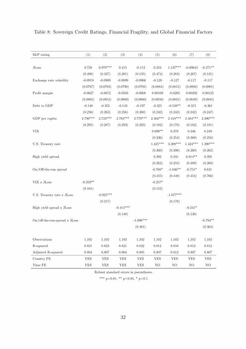
Table 8: Sovereign Credit Ratings, Financial Fragility, and Global Financial Factors

S&P rating (1) (2) (3) (4) (5) (6) (7) (8)

JLoss 0.728 0.978*** 0.415 -0.113 0.324 1.137*** -0.00644 -0.271**

(0.498) (0.327) (0.291) (0.135) (0.474) (0.283) (0.267) (0.121)

Exchange rate volatility -0.0919 -0.0909 -0.0899 -0.0906 -0.120 -0.127 -0.117 -0.117

(0.0787) (0.0793) (0.0790) (0.0792) (0.0884) (0.0812) (0.0893) (0.0901)

Profit margin -0.0627 -0.0672 -0.0593 -0.0608 0.00169 -0.0205 0.00492 0.00125

(0.0865) (0.0854) (0.0869) (0.0860) (0.0850) (0.0831) (0.0849) (0.0845)

Debt to GDP -0.146 -0.355 -0.143 -0.197 -0.321 -0.549** -0.315 -0.361

(0.256) (0.263) (0.256) (0.260) (0.242) (0.243) (0.242) (0.247)

GDP per capita 2.790*** 2.723*** 2.783*** 2.779*** 2.402*** 2.418*** 2.404*** 2.390***

(0.295) (0.287) (0.293) (0.293) (0.182) (0.178) (0.182) (0.181)

VIX 0.690** 0.378 0.246 0.249

(0.336) (0.254) (0.260) (0.258)

U.S. Treasury rate 1.425*** 3.309*** 1.424*** 1.390***

(0.260) (0.396) (0.260) (0.262)

High yield spread 0.392 0.341 0.814** 0.395

(0.262) (0.255) (0.389) (0.260)

On/Off-the-run spread -0.768* -1.046** -0.751* 0.631

(0.455) (0.448) (0.454) (0.766)

VIX x JLoss -0.359** -0.257*

(0.161) (0.152)

U.S. Treasury rate x JLoss -0.925*** -1.077***

(0.217) (0.178)

High yield spread x JLoss -0.414*** -0.241*

(0.148) (0.136)

On/off-the-run-spread x JLoss -1.096*** -0.794**

(0.401) (0.364)

Observations 1,102 1,102 1,102 1,102 1,102 1,102 1,102 1,102

R-squared 0.821 0.823 0.821 0.822 0.812 0.816 0.812 0.812

Adjusted R-squared 0.804 0.807 0.804 0.805 0.807 0.812 0.807 0.807

Country FE YES YES YES YES YES YES YES YES

Time FE YES YES YES YES NO NO NO NO

Robust standard errors in parentheses.

*** p<0.01, ** p<0.05, * p<0.1

32

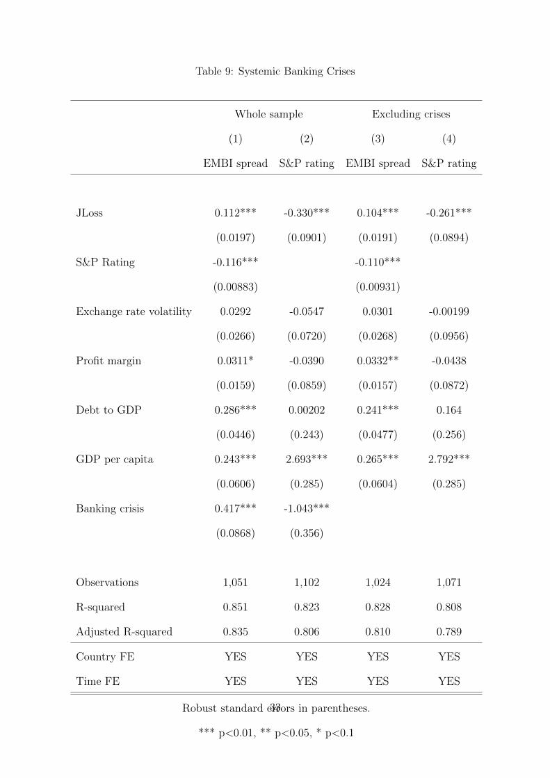
Table 9: Systemic Banking Crises

Whole sample Excluding crises

(1) (2) (3) (4)

EMBI spread S&P rating EMBI spread S&P rating

JLoss 0.112*** -0.330*** 0.104*** -0.261***

(0.0197) (0.0901) (0.0191) (0.0894)

S&P Rating -0.116*** -0.110***

(0.00883) (0.00931)

Exchange rate volatility 0.0292 -0.0547 0.0301 -0.00199

(0.0266) (0.0720) (0.0268) (0.0956)

Profit margin 0.0311* -0.0390 0.0332** -0.0438

(0.0159) (0.0859) (0.0157) (0.0872)

Debt to GDP 0.286*** 0.00202 0.241*** 0.164

(0.0446) (0.243) (0.0477) (0.256)

GDP per capita 0.243*** 2.693*** 0.265*** 2.792***

(0.0606) (0.285) (0.0604) (0.285)

Banking crisis 0.417*** -1.043***

(0.0868) (0.356)

Observations 1,051 1,102 1,024 1,071

R-squared 0.851 0.823 0.828 0.808

Adjusted R-squared 0.835 0.806 0.810 0.789

Country FE YES YES YES YES

Time FE YES YES YES YES

Robust standard errors in parentheses.

*** p<0.01, ** p<0.05, * p<0.1

33

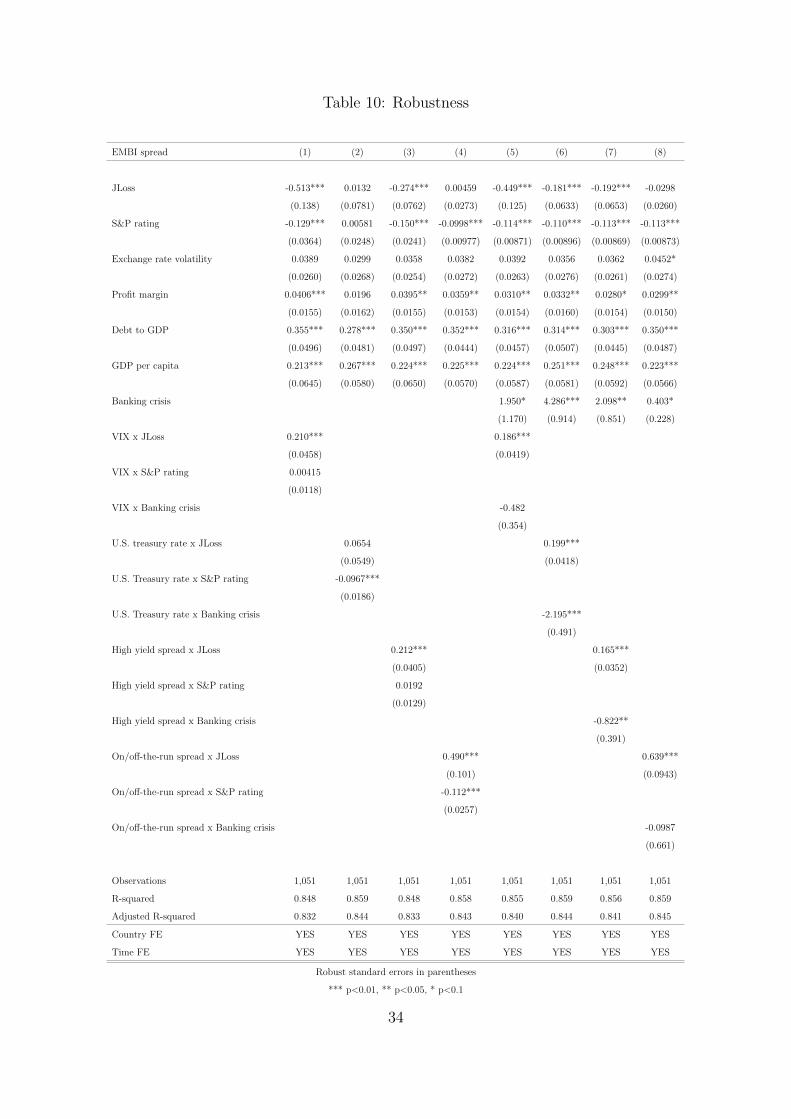
Table 10: Robustness

EMBI spread (1) (2) (3) (4) (5) (6) (7) (8)

JLoss -0.513*** 0.0132 -0.274*** 0.00459 -0.449*** -0.181*** -0.192*** -0.0298

(0.138) (0.0781) (0.0762) (0.0273) (0.125) (0.0633) (0.0653) (0.0260)

S&P rating -0.129*** 0.00581 -0.150*** -0.0998*** -0.114*** -0.110*** -0.113*** -0.113***

(0.0364) (0.0248) (0.0241) (0.00977) (0.00871) (0.00896) (0.00869) (0.00873)

Exchange rate volatility 0.0389 0.0299 0.0358 0.0382 0.0392 0.0356 0.0362 0.0452*

(0.0260) (0.0268) (0.0254) (0.0272) (0.0263) (0.0276) (0.0261) (0.0274)

Profit margin 0.0406*** 0.0196 0.0395** 0.0359** 0.0310** 0.0332** 0.0280* 0.0299**

(0.0155) (0.0162) (0.0155) (0.0153) (0.0154) (0.0160) (0.0154) (0.0150)

Debt to GDP 0.355*** 0.278*** 0.350*** 0.352*** 0.316*** 0.314*** 0.303*** 0.350***

(0.0496) (0.0481) (0.0497) (0.0444) (0.0457) (0.0507) (0.0445) (0.0487)

GDP per capita 0.213*** 0.267*** 0.224*** 0.225*** 0.224*** 0.251*** 0.248*** 0.223***

(0.0645) (0.0580) (0.0650) (0.0570) (0.0587) (0.0581) (0.0592) (0.0566)

Banking crisis 1.950* 4.286*** 2.098** 0.403*

(1.170) (0.914) (0.851) (0.228)

VIX x JLoss 0.210*** 0.186***

(0.0458) (0.0419)

VIX x S&P rating 0.00415

(0.0118)

VIX x Banking crisis -0.482

(0.354)

U.S. treasury rate x JLoss 0.0654 0.199***

(0.0549) (0.0418)

U.S. Treasury rate x S&P rating -0.0967***

(0.0186)

U.S. Treasury rate x Banking crisis -2.195***

(0.491)

High yield spread x JLoss 0.212*** 0.165***

(0.0405) (0.0352)

High yield spread x S&P rating 0.0192

(0.0129)

High yield spread x Banking crisis -0.822**

(0.391)

On/off-the-run spread x JLoss 0.490*** 0.639***

(0.101) (0.0943)

On/off-the-run spread x S&P rating -0.112***

(0.0257)

On/off-the-run spread x Banking crisis -0.0987

(0.661)

Observations 1,051 1,051 1,051 1,051 1,051 1,051 1,051 1,051

R-squared 0.848 0.859 0.848 0.858 0.855 0.859 0.856 0.859

Adjusted R-squared 0.832 0.844 0.833 0.843 0.840 0.844 0.841 0.845

Country FE YES YES YES YES YES YES YES YES

Time FE YES YES YES YES YES YES YES YES

Robust standard errors in parentheses

*** p<0.01, ** p<0.05, * p<0.1

34

Figures

Inputs:• Probability of

default• Exposure• Correlations

Output:• Implied

probability density of joint losses

Saddle point method

Step 1:• Random Variable

Laplace transformation

Step 2:• Moment

generating functions (MGM)

Bromwich integral

Step 3:• Probability density

of losses

Martin (2001) calculations:• Marginal

contribution to risk• Expected and

unexpected losses

𝑃 =

𝑖=1

𝑁

𝑒𝑖 ∙ 1Ι𝐷𝑖

Jloss computation:𝐽𝑙𝑜𝑠𝑠𝑖,𝑡

=σ𝐽=1𝑁 𝑇𝑜𝑡𝑎𝑙 𝑙𝑜𝑠𝑠𝑒𝑠𝑗,𝑡

σ𝐽=1𝑁 𝐸𝑥𝑝𝑜𝑠𝑢𝑟𝑒𝑗,𝑡

Figure 1: JLoss Methology

35

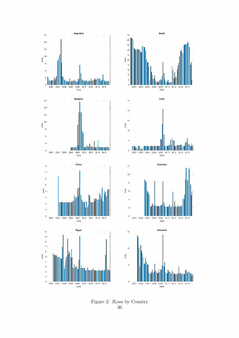
Figure 2: JLoss by Country36

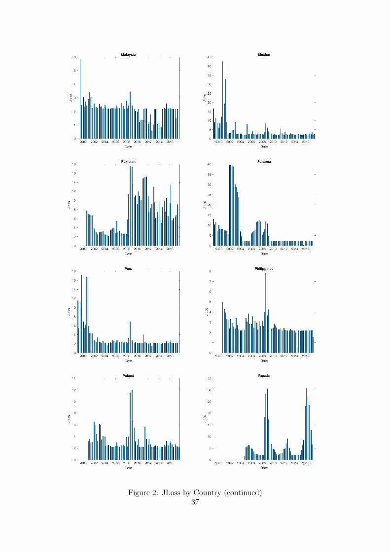
Figure 2: JLoss by Country (continued)37

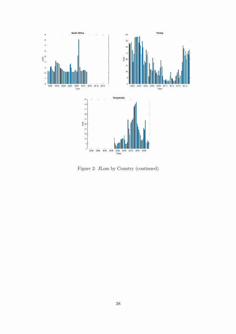
Figure 2: JLoss by Country (continued)

38

Appendix A

Table A.1 Banks per Country

Country Number of banks

Argentina 6

Brazil 14

Bulgaria 4

Chile 9

China 40

Colombia 7

Egypt 10

Indonesia 40

Malaysia 8

Mexico 6

Pakistan 21

Panama 7

Peru 22

Philippines 19

Poland 13

Russia 46

South Africa 7

Turkey 13

Venezuela 6

39

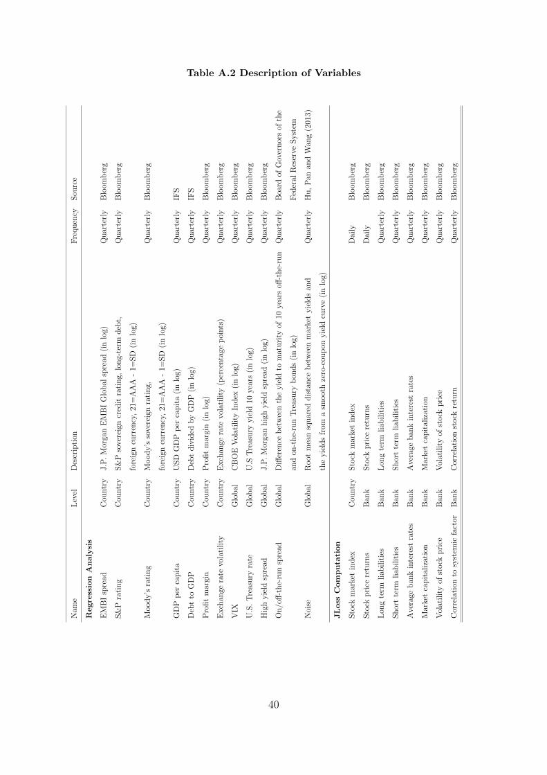
Table A.2 Description of VariablesN

ame

Lev

elD

escr

ipti

onF

requen

cySou

rce

Regre

ssio

nA

naly

sis

EM

BI

spre

adC

ountr

yJ.P

.M

orga

nE

MB

IG

lobal

spre

ad(i

nlo

g)Q

uar

terl

yB

loom

ber

g

S&

Pra

ting

Cou

ntr

yS&

Pso

vere

ign

cred

itra

ting,

long-

term

deb

t,Q

uar

terl

yB

loom

ber

g

fore

ign

curr

ency

,21

=A

AA

-1=

SD

(in

log)

Moody’s

rati

ng

Cou

ntr

yM

oody’s

sove

reig

nra

ting,

Quar

terl

yB

loom

ber

g

fore

ign

curr

ency

,21

=A

AA

-1=

SD

(in

log)

GD

Pp

erca

pit

aC

ountr

yU

SD

GD

Pp

erca

pit

a(i

nlo

g)Q

uar

terl

yIF

S

Deb

tto

GD

PC

ountr

yD

ebt

div

ided

by

GD

P(i

nlo

g)Q

uar

terl

yIF

S

Pro

fit

mar

gin

Cou

ntr

yP

rofit

mar

gin

(in

log)

Quar

terl

yB

loom

ber

g

Exch

ange

rate

vola

tility

Cou

ntr

yE

xch

ange

rate

vola

tility

(per

centa

gep

oints

)Q

uar

terl

yB

loom

ber

g

VIX

Glo

bal

CB

OE

Vol

atilit

yIn

dex

(in

log)

Quar

terl

yB

loom

ber

g

U.S

.T

reas

ury

rate

Glo

bal

U.S

Tre

asury

yie

ld10

year

s(i

nlo

g)Q

uar

terl

yB

loom

ber

g

Hig

hyie

ldsp

read

Glo

bal

J.P

.M

orga

nhig

hyie

ldsp

read

(in

log)

Quar

terl

yB

loom

ber

g

On/o

ff-t

he-

run

spre

adG

lobal

Diff

eren

ceb

etw

een

the

yie

ldto

mat

uri

tyof

10ye

ars

off-t

he-

run

Quar

terl

yB

oard

ofG

over

nor

sof

the

and

on-t

he-

run

Tre

asury

bon

ds

(in

log)

Fed

eral

Res

erve

Syst

em

Noi

seG

lobal

Root

mea

nsq

uar

eddis

tance

bet

wee

nm

arke

tyie

lds

and

Quar

terl

yH

u,

Pan

and

Wan

g(2

013)

the

yie

lds

from

asm

oot

hze

ro-c

oup

onyie

ldcu

rve

(in

log)

JL

oss

Com

puta

tion

Sto

ckm

arke

tin

dex

Cou

ntr

ySto

ckm

arke

tin

dex

Dai

lyB

loom

ber

g

Sto

ckpri

cere

turn

sB

ank

Sto

ckpri

cere

turn

sD

aily

Blo

omb

erg

Lon

gte

rmliab

ilit

ies

Ban

kL

ong

term

liab

ilit

ies

Quar

terl

yB

loom

ber

g

Shor

tte

rmliab

ilit

ies

Ban

kShor

tte

rmliab

ilit

ies

Quar

terl

yB

loom

ber

g

Ave

rage

ban

kin

tere

stra

tes

Ban

kA

vera

geban

kin

tere

stra

tes

Quar

terl

yB

loom

ber

g

Mar

ket

capit

aliz

atio

nB

ank

Mar

ket

capit

aliz

atio

nQ

uar

terl

yB

loom

ber

g

Vol

atilit

yof

stock

pri

ceB

ank

Vol

atilit

yof

stock

pri

ceQ

uar

terl

yB

loom

ber

g

Cor

rela

tion

tosy

stem

icfa

ctor

Ban

kC

orre

lati

onst

ock

retu

rnQ

uar

terl

yB

loom

ber

g

40

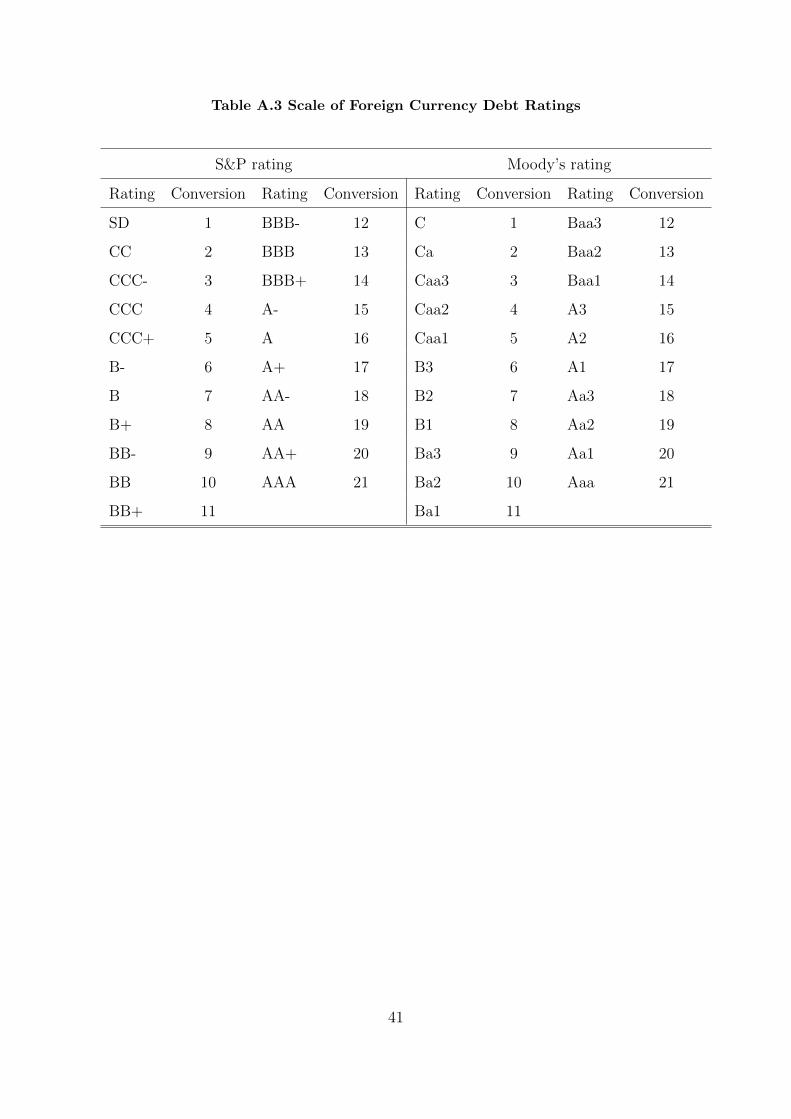
Table A.3 Scale of Foreign Currency Debt Ratings

S&P rating Moody’s rating

Rating Conversion Rating Conversion Rating Conversion Rating Conversion

SD 1 BBB- 12 C 1 Baa3 12

CC 2 BBB 13 Ca 2 Baa2 13

CCC- 3 BBB+ 14 Caa3 3 Baa1 14

CCC 4 A- 15 Caa2 4 A3 15

CCC+ 5 A 16 Caa1 5 A2 16

B- 6 A+ 17 B3 6 A1 17

B 7 AA- 18 B2 7 Aa3 18

B+ 8 AA 19 B1 8 Aa2 19

BB- 9 AA+ 20 Ba3 9 Aa1 20

BB 10 AAA 21 Ba2 10 Aaa 21

BB+ 11 Ba1 11

41