Embed Size (px)
Citation preview

Policy Research Working Paper 9906
Sovereign Bonds since WaterlooJosefin Meyer
Carmen M. Reinhart Christoph Trebesch
Development Economics Vice PresidencyOffice of the Senior Vice President and Chief EconomistJanuary 2022
Pub
lic D
iscl
osur
e A
utho
rized
Pub
lic D
iscl
osur
e A
utho
rized
Pub
lic D
iscl
osur
e A
utho
rized
Pub
lic D
iscl
osur
e A
utho
rized
Produced by the Research Support Team
Abstract
The Policy Research Working Paper Series disseminates the findings of work in progress to encourage the exchange of ideas about development issues. An objective of the series is to get the findings out quickly, even if the presentations are less than fully polished. The papers carry the names of the authors and should be cited accordingly. The findings, interpretations, and conclusions expressed in this paper are entirely those of the authors. They do not necessarily represent the views of the International Bank for Reconstruction and Development/World Bank and its affiliated organizations, or those of the Executive Directors of the World Bank or the governments they represent.
Policy Research Working Paper 9906
This paper studies external sovereign bonds as an asset class. It compiles a new database of 266,000 monthly prices of foreign-currency government bonds traded in London and New York between 1815 (the Battle of Waterloo) and 2016, covering up to 91 countries. The main insight is that, as in equity markets, the returns on external sovereign bonds have been sufficiently high to compensate for risk. Real ex-post returns average more than 6 percent annually across two centuries, including default episodes, major wars, and global crises. This represents an excess return of 3–4 percent
above US or UK government bonds, which is comparable to stocks and outperforms corporate bonds. Central to this finding are the high average coupons offered on external sovereign bonds. The observed returns are hard to reconcile with canonical theoretical models and the degree of credit risk in this market, as measured by historical default and recovery rates. Based on an archive of more than 300 sover-eign debt restructurings since 1815, the authors show that full repudiation is rare; the median creditor loss (haircut) is below 50 percent.
This paper is a product of the Office of the Senior Vice President and Chief Economist, Development Economics Vice Presidency. It is part of a larger effort by the World Bank to provide open access to its research and make a contribution to development policy discussions around the world. Policy Research Working Papers are also posted on the Web at http://www.worldbank.org/prwp. The authors may be contacted at [email protected]; [email protected]; and [email protected].
Sovereign Bonds since Waterloo
Josefin Meyer (DIW Berlin, Kiel Institute and CEPR)
Carmen M. Reinhart (Harvard University, CEPR and NBER)
Christoph Trebesch (Kiel Institute and CEPR)1
JEL codes: E4, F3, F4, G1, N0
1 We received very helpful comments from Laura Alfaro, Darrell Duffie, Rui Esteves, Gita Gopinath, Şebnem Kalemli-Özcan, Sam Langfield, Matteo Maggiori, Vincent Reinhart, Moritz Schularick, Frank Westermann and from conference participants at the NBER IFM Summer Institute 2018, the ASSA Meetings 2015, the Macrohistory Workshop in Bonn, the Sovereign Debt Conference in Zurich, DebtCon2 in Geneva, the Financial Crises conference at the LSE, as well as at seminars at UC Berkeley, Harvard, LUISS, EIEF, and at the Universities of Cologne, Frankfurt, Humboldt, Melbourne, Munich and Oxford. We also thank the editors and four anonymous referees for many helpful suggestions. Melanie Baade, Angelica Dominguez, Carl Hallmann, Moritz Müller-Freitag, Clemens Graf von Luckner, Khanh Phuong Ho, Tim Hofstetter, Torge Marxsen, Philipp Nickol, Maximilian Rupps, Sebastian Rieger, Paul Röttger, Christopher Schang and Julian Wichert provided excellent research assistance. We thank Julian Schumacher for sharing data on missed payments in recent bond defaults. Josefin Meyer gratefully acknowledges support by the European Commission’s Marie Curie Fellowship Programme under REA grant agreement no. 608129. Christoph Trebesch gratefully acknowledges financial support from the DFG Priority Programme “Experience and Expectation: Historical Foundations of Economic Behaviour” (SPP 1859) and from the Junior Researcher Fund of LMU München. All remaining errors are our own. Contact: [email protected]; [email protected]; [email protected].

1
1. Introduction
The battle of Waterloo in 1815 can be seen as the birthday of modern sovereign debt markets - and of
their recurring boom-bust cycles. The Napoleonic Wars and the defeat of France and Spain accelerated
the independence of a dozen new republics in Latin America, which quickly sought financing in London.
The first emerging market debt boom, which also included the first Greek international bond, among
others, ended abruptly in the financial panic of 1825. Since then, many similar cycles of lending and
default have followed, often involving the same countries, again and again.
Given the frequent defaults and limited enforcement of external sovereign debt, why are investors
attracted to this asset class? We tackle this question by examining how creditors have fared in sovereign
debt markets over the short and long run with a focus on financial returns. 2 Two components are necessary
to calculate total bond returns. The first of these is the price series. We collected monthly price quotations
of 1,552 foreign-currency bonds issued and traded in London and New York over the past 200 years, with
a total of 266,134 observations covering up to 91 countries, in an unbalanced sample. 3 Because of the
recurring credit events of many of the sovereigns, prices and bond characteristics are necessary but not
sufficient to calculate returns. The second required component is to quantify the investor losses due to
sovereign default and debt restructurings (“haircuts”), for which we have compiled an extensive database
covering missed payments, debt renegotiation terms, and face value write-downs in more than 300 debt
crisis episodes since 1815. 4
We find that the ex-post returns on foreign-currency sovereign bonds compensate investors for the risks
they face. Notwithstanding the defaults, wars, and global crises over the past two centuries, the average
real yearly ex-post return on a global portfolio of external sovereign bonds was 6.9%. Thus, an investor
entering this market with a one-year horizon can expect to receive on average a real ex-post return of
almost 7% – about 4% higher than that of the “risk-free” benchmark of UK or US government bonds. 5
Excess returns are driven by the high coupons offered in this market. Not surprisingly, returns tend to be
2 External debt is defined here by currency rather than jurisdiction of issuance or residency of ownership. We focus on British pound and US dollar debt instruments and place of issue and trading (only those traded in London and/or New York). Hence, sample selection for our pricing data is not dictated by any priors other than location. Specifically, we start with emerging markets today and then move backward, adding sovereigns that have tapped London and New York markets in the past, including many of today’s advanced countries such as Australia, Canada, Germany, Greece, Italy, Japan, Portugal, and Spain. 3 London and New York were the two dominant trading centers in the 200-year sample (Michie 1987). Our country sample starts with about a dozen countries in the early19th century and grows over time, with gaps for individual countries and eras (especially the gap of the “syndicated loan era” of the 1970s and 1980s). 4 We use the term “haircut” to describe the size of creditor losses suffered in a sovereign default and debt restructuring. This wording is in line with the international macro and sovereign debt literature (e.g., Sturzenegger and Zettelmeyer 2008; Aguiar and Amador 2014). In finance, the term “haircut” is sometimes used differently, typically referring to a “repo haircut,” that is, the discount on the face value of an asset when valuing it as collateral in a repo transaction (Gorton and Metrick 2012). 5 These results, on the whole, show a higher rate of return for this asset class than a number of the earlier studies, which are mostly based on a different methodology and a more limited sample of sovereign bonds. See Section 2.

2
lower in crisis-prone decades. Furthermore, the risk-return properties are in line with those of other
tradable assets, in particular US and UK equities for which we also compute returns over the 200-year
sample.
The results go a long way in solving a puzzle that has preoccupied the literature for decades – namely,
why sovereigns can borrow again despite a history of default (Reinhart, Rogoff, and Savastano 2003;
Cruces and Trebesch 2013). 6 High-risk countries that defaulted often manage to place bonds quickly post-
default. In 2016, Argentina re-accessed international markets only months after exiting its seventh default.
The new issues included a 100-year bond, which led market observers to conclude that credit markets
were overheating. 7 In the past years, Africa had its own issuance boom, as formerly highly indebted poor
countries (HIPCs) such as Ghana or Zambia easily placed bonds abroad. Our historical results help to
make sense of these market outcomes, as this asset class is characterized by a high return-to-risk ratio.
This helps our understanding of why sovereign debtors can undergo repeated cycles of over-borrowing,
often followed by default and a subsequent market re-entry (i.e., serial default).
Our paper departs from the literature on sovereign debt in three main ways. First, we take a different
perspective – that of an investor. The bulk of the existing work takes the borrowing countries’ perspective,
often focusing on the determinants and costs of default. 8 The second is the extensive time span and
geographical coverage of our study; earlier work on creditor returns has studied short samples or a limited
number of countries. The third is the granularity of our data, as we trace the financial history of more than
1,500 individual bonds at a monthly level, combining historical data on bond prices, coupon payments,
and haircuts due to default. The result is the most ambitious dataset of sovereign debt to date, taking
further the work of Lindert and Morton (1989), Homer and Sylla (2005), and Obstfeld and Taylor (2005),
among others.
We are the first to quantify the returns on external sovereign bonds with long-run pricing data, despite the
fact that this is one of the largest and oldest asset classes worldwide. 9 The likely explanation is data
limitations. Studies on long-run asset returns typically use annual data of representative benchmark bonds
or aggregate indices (e.g., Dimson, Marsh, and Staunten 2001; Jordà et al. 2017). 10 This standard
6 Eaton and Gersovitz (1981), among others, assume permanent exclusion after a sovereign default, which is at odds with the data (see also Aguiar and Gopinath 2006; Panizza, Sturzenegger, and Zettelmeyer 2009; and Cruces and Trebesch 2013). 7 See Financial Times, June 22, 2017, “The rush for Argentina’s 100-year bond points to an investment bubble.” 8 For surveys, see Panizza, Sturzenegger, and Zettelmeyer (2009), Aguiar and Amador (2014) and Mitchener and Trebesch (2021). 9 Historically, bonds issued by foreign governments accounted for about 10% of all financial assets trading in London (Michie 2001). Today, foreign-currency sovereign bonds continue to be a dominant asset class, especially for emerging markets. For 2017, the BIS reports a stock of US$1.9 trillion of external sovereign bonds (BIS 2018), about the same as total German government debt or about 10% of total gross US government debt. 10 Dimson, Marsh, and Staunten (2001) gather annual data on equities, bonds, and bills for 16 countries back to 1900. Their data on government bonds mostly builds on representative domestic currency instruments. Jordá et al. (2017) compile yearly country-level indices of asset returns, 1870-2015, for 16 countries, including housing.

3
approach, however, is not viable for external sovereign debt, due to the many defaults in this market and
because defaults come in different varieties and can affect bonds differently, resulting in heterogeneous
outcomes (Meyer 2021). A rigorous calculation of total returns on external sovereign bonds thus requires
pricing data as well as details on the fate of each bond in default, in particular on the timing and scope of
missed payments and detailed restructuring terms. This type of bond-level default data is much harder to
collect and was not readily available prior to this study.
The second main building block is our new archive of external default and restructuring events. We
compute creditor losses (haircuts) bond-by-bond and deal-by-deal and combine the information on
restructuring outcomes with our monthly bond price data. Moreover, we trace missed or partial bond
payments at a monthly frequency. Because, as we establish here, coupons are the main driver of total
returns in this market, it is important to measure interest payments accurately, especially during lengthy
default spells. What the data reveal is that sovereigns in default on principal payments often continue to
service coupons in full or in part, which pushes up investor returns. Moreover, coupon payments on the
same bond can vary markedly over the course of a crisis. The granular repayment track record thus allows
us to build monthly total return series on a bond-by-bond basis in a consistent manner, as well as
representative country and global portfolios over long time spans.
Thirdly, we compile an extensive supplementary database that provides unique insights into the liquidity
of this asset class. We gathered monthly, bond-level bid-ask spreads over two centuries, covering 62% of
our pricing sample (in total 165,638 observations, see Figure B3).
Our results are hard to reconcile with seminal quantitative models of sovereign default. Until recently,
this literature assumed risk-neutral investors and sovereign risk premia that solely reflect the expected
losses from default (e.g., Aguiar and Gopinath 2006; Arellano 2008; Mendoza and Yue 2012). When
investors are risk-neutral, excess return above “risk-free” bonds should be zero in expectation. Yet, we
find real excess returns that are in the range of 2% to 4% ex-post for the full global sample, although there
is considerable time variation. Thus, investors typically receive a compensatory premium for holding
sovereign risk that exceeds historical credit losses. This finding gives support to a growing body of
quantitative work that assumes risk-averse (or uncertainty averse) creditors in this market. 11
The high returns we observe cannot be easily explained by historical default and recovery rates. Using
our new default and restructuring database, we show that sovereign defaults do not usually wipe out the
claims of private creditors. Almost all the defaults over the past 200 years have been solved by a debt
exchange of old into new debt at a discount – with an average haircut of 44% and a standard deviation of
Compared to these studies, we zoom in on one asset class and cover 91 countries, 200 years at monthly frequency, and instrument-level data. 11 See Barro’s discussion of rare disasters with Epstein-Zin preferences (Barro 2006) and, more recently, Broner, Lorenzoni, and Schmukler (2013), Lizarazo (2013), Borri and Verdelhan (2015), Aguiar et al. (2016), Grosse Steffen and Podstawski (2016), Pouzo and Presno (2016), and Asonuma and Joo (2018).
4
30%. Moreover, we find that bond prices often recover relatively quickly during and after default spells,
although the variation across episodes is also large. On average, creditors recoup their pre-crisis
investment (measured one year before) within five years after the default; and in 25% of cases (upper
quartile), investors recover their losses in less than one year. There are, of course, outlier episodes
involving major upheavals such as wars, revolutions, or the break-up of empires (e.g., in Austria-Hungary,
China, or Russia). However, in the majority of debt crises, investor losses are partial. Debt repudiation
cases are comparatively rare.
On a more general level, our results reveal many parallels to the case of equity. As is the case for stocks,
we find that sovereign external bonds show high excess returns coupled with a relatively low return
volatility. The seminal work by Mehra and Prescott (1985) showed that standard asset pricing models are
not able to reproduce the large empirically observed wedge between risky and riskless assets. Their
contribution was followed by a stream of studies on the equity premium puzzle, largely focusing on the
United States after World War II (WW2) (see Kocherlakota 1996; Campbell 2003). Compared to the
literature on long-run equity returns, our analysis of external bonds covers far more countries, particularly
encompassing emerging markets and developing countries. It also goes much further back. 12 There are,
however, gaps in the bond pricing series of individual countries, and the market for external sovereign
bonds shrinks in the Bretton Woods era of capital controls, and all but disappears during the syndicated
bank lending spell of the 1970s and 1980s (our average country coverage is 70 years). There is also
research on the “credit spread puzzle” for corporate bonds, typically using data from the past 30 years. 13
The high excess returns on external sovereign bonds have received much less attention, in large part
because earlier studies found little evidence of excess returns in the first place (Section 2).
Because we quantify the outcome of each default episode, our analysis moves away from the typical
binary approach in the literature where a country is either in default or it is not. Like for currency or
inflation crises, orders of magnitude matter. We measure the magnitude of these “credit events” both in
terms of haircuts and in terms of amounts in default, which allows identifying the shades of gray across
countries and time. 14 The data show that credit events in this market are best described as partial defaults
with re-contracting, in the spirit of Bulow and Rogoff (1989), rather than as full defaults, as is typically
12 Barro and Ursua (2008) use returns data starting in the late 19th century for about 30 countries using Global Financial Data (GFD) as source. Dimson, Marsh, and Staunton (2001) and Jordà et al. (2017) cover 16 countries, starting in 1900 and 1870, respectively. All three contributions use annual data, as do Mehra and Prescott (1985), who focus on the United States, 1889-1978. We use monthly data and start in 1815, with a country sample starting from a dozen in the 19th century and growing over time. 13 Chen, Collin-Dufresne, and Goldstein (2009) and Chen (2010) study the credit spread puzzle for corporate debt and summarize the literature on this issue. Asquith, Mullins, and Wolff (1989) is an early study on the high excess returns on US junk bonds. 14 There is already ample data on the occurrence and duration of sovereign defaults (e.g., Standard and Poor’s 2006, Reinhart and Rogoff 2009, or Asonuma and Trebesch 2016), but there is no long-run dataset on sovereign recovery rates thus far.
5
assumed (e.g., Eaton and Gersovitz 1981, Aguiar and Gopinath 2006, Arellano 2008, Broner, Martin, and
Ventura 2010).
Finally, our study is the first to offer a 200-year perspective of sovereign bond pricing. Compared with
Mauro, Sussman, and Yafeh (2002), for example, we add 60 years of data pre-1870, as well as the entire
spell before, during, and after WW1 and WW2, when co-movement in sovereign bond prices was higher
than in the relatively tranquil pre-1913 spell. Our 200-year dataset has a monthly frequency and can be
explored at the global, country, and bond levels.
The paper proceeds as follows. In the next section, we review the related literature, especially work
measuring sovereign haircuts and investor returns. Section 3 describes credit events and investor losses
(haircuts) on external sovereign debt across two centuries, while Section 4 moves beyond defaults and
documents the history of sovereign bond prices and returns over the very long run. Section 5 explores the
behavior of returns around debt crises to understand investors’ recoveries in this market. Section 6 focuses
on risk-return comparisons across asset classes. Section 7 concludes and lays a path for future research.
2. Previous studies: Sovereign debt returns and haircuts
The related literature can be broadly grouped into two categories: papers that quantify rates of return on
sovereign debt or related emerging market investments and a literature that provides estimates of haircuts
and recovery rates for sovereign credit events. By and large, our results on bond returns and haircuts turn
out to be similar to the existing body of work, whenever meaningful comparisons are possible. The main
contribution is to provide a much more comprehensive picture, covering all countries for which external
bond data were available and spanning the complete 200-year picture.
In the literature on investor returns, several earlier papers calculate internal rates of return (IRRs) to assess
how creditors have fared in sovereign debt markets (i.e., until the bond is extinguished). IRRs take the
perspective of a buy-and-hold investor and discount cash flows over the life span of a debt instrument
(from issuance until maturity or sample end). 15 IRRs have the benefit that they do not require collecting
market prices, so that they can be calculated for all types of instruments, even for bonds not traded on the
market. The main drawback of IRRs is that, despite requiring much data work, they provide only one data
point per instrument, namely the bond’s return over the entire holding period. Indeed, IRRs assume that
investors buy a sovereign bond instrument at issuance and never sell it. This is unlikely to be true for most
investors, today and also prior to WW2 when sovereign bond maturities typically exceeded 30 years.
Price-based returns are a more flexible measure and can be used to address a much broader range of
15 Specifically, IRRs (or 𝑟𝑟𝐼𝐼𝐼𝐼𝐼𝐼) can be extracted from the cash flow data to yield a net present value of zero, as follows: 0 = 𝑁𝑁𝑁𝑁𝑁𝑁 = −𝑁𝑁0 + ∑ 𝐶𝐶𝐶𝐶𝑡𝑡
(1+𝑟𝑟𝐼𝐼𝐼𝐼𝐼𝐼)𝑡𝑡𝑇𝑇𝑡𝑡=1 , where 𝑇𝑇 is bond maturity, 𝐶𝐶𝐶𝐶𝑡𝑡 are debt payments (coupon and amortization) in
year 𝑡𝑡, and 𝑁𝑁0 is the purchasing price, that is, the issue price of the bond.

6
research questions. Most obviously, price-based returns can be traced over time, by computing time series
of daily, monthly, or yearly returns.
Lindert and Morton (1989) conducted the most comprehensive study on long-run sovereign bond returns
thus far. They compute IRRs for 10 countries between 1850 and 1983, covering more than 1,000
sovereign, sub-sovereign, and corporate bond instruments. They find average realized nominal returns of
4.5%, realized real returns of 2.5%, and excess returns of 0.4%. In Appendix B3.1, we compare our results
with theirs in detail and present a conceptual section on the different return measures (using their data as
cleaned by Esteves [2013]). At the bond level, we find very similar results when comparing IRRs with
price-based holding period returns. At the aggregate level, however, the reported averages by Lindert and
Morton (1989) are lower, for two reasons that are less of a concern in our analysis. First, two outliers
(Russia and Turkey) decrease the average return in their sample. After WW1, both countries entered
defaults that took decades to resolve, due to Russia’s Communist revolution and the breakup of the
Ottoman Empire, respectively. In our much broader sample, outliers and lengthy defaults of individual
bonds carry less weight. Second, Lindert and Morton (1989) include municipal and corporate bonds,
which leads to lower aggregate returns, as we show in the appendix. We focus on sovereign bonds only,
which have higher returns, on average. Another reason why their averages seem lower is that Lindert and
Morton (1989) show buy-and-hold returns only, while we focus on average annual portfolio returns, as is
standard in the finance literature. We nevertheless show geometric returns throughout our paper and
researchers using our dataset can compute holding period returns for any period of their choosing.
Eichengreen and Portes (1988, 1991) focus on the interwar years and show that these were a bad period
for investing in external bonds. Over the decade of the 1920s, nominal rates of return were around 4%-
5%, which is similar to what we find in the 1920s and only slightly higher than the returns on UK or US
government bonds. 16 For an era that predates our Waterloo starting point, Drelichman and Voth (2011)
also calculate IRRs and find substantive (profitable) returns on short-term loans to King Philipp II of
Habsburg Spain, despite his notorious serial defaults. 17
Klingen, Weder, and Zettelmeyer (2004) study the return performance of sovereign debt in a large sample
of developing countries between 1970 and 2000, including, importantly, the dominant form of lending in
that era, syndicated bank loans. To estimate returns they use aggregate bank and bond flows, public and
16 These averages combine sovereign, sub-sovereign (e.g., regional), and corporate bonds. Less than 20% of bonds in Eichengreen and Portes (1988, 1991) were issued by a sovereign. 17 There is also a literature studying the overall portfolio return of British overseas investments before WW1 using price data, but with no emphasis on sovereign debt. Edelstein (1982) finds that British investors gained a higher return abroad than at home, using returns on 566 foreign stocks and bonds (private and sovereign), 1870-1913. Goetzman and Ukhow (2006) use the same data but apply modern portfolio theory. Chabot and Kurz (2010) compute returns on more than 4,000 stocks and bonds (private and sovereign) trading in the United Kingdom and the United States during 1866-1907. They report significant excess returns on foreign government bonds compared with UK government bonds. None of these contributions mentions how the numerous sovereign defaults and restructurings are accounted for.

7
private. On average, they find a 9% nominal return, comparable to that of US Treasury bonds at that time
(zero premia), but there is substantial time variation. Appendix B3.2 shows that we get very similar results
in those subsamples of their dataset for which pricing data exist. Furthermore, in Appendix B4, we add
evidence on the 1970s, 1980s, and early 1990s, partly based on secondary market price data for syndicated
loans 1985-1993. The results confirm those in Klingen, Weder, and Zettelmeyer (2004): sovereign debt
returns were very low in the late 1980s and very high in the early 1990s.
Following large-scale debt restructurings in the early 1990s under the Brady Plan, fixed income markets
reemerged as a dominant source of credit to emerging markets. The recent literature mostly explores this
post-1990 sovereign bond era with an approach closer in spirit to the one developed in this paper, typically
using JP Morgan’s Emerging Markets Bond Index (EMBI) country series (e.g., Broner, Lorenzoni, and
Schmukler 2013; Borri and Verdelhan 2015; Andritzky and Schumacher 2018). 18 The results highlight
excess returns by country in the 3%-15% range, which is significantly higher than those reported by papers
studying the pre-1990s and in line with our results.
A broad takeaway from this previous literature on bond returns is that, historically, emerging market debt
delivered returns that were only slightly above the risk-free rate. This made it all the more puzzling why
investors continue to flock to this asset class in their search for high yield. Compared with that body of
research, we provide a more representative and encompassing picture of the external sovereign bond
market. Our bigger sample gives less weight to individual defaulters (like Russia) or episodes that were
particularly turbulent (like the Great Depression). We also disregard the (lower) returns of sub-sovereign
bonds. Instead, we focus on external sovereign bonds and include all episodes for which price quotations
exist, including spells with very high returns in the aftermath of wars and crises, as well as during the
boom decades of the 1840s, 1860s, 1880s, 1940s, 1950s, 1990s, and the 2000s (many of these were not
included in previous studies).
A necessary ingredient for the calculation of ex-post returns is to account for losses due to default or
restructuring, which requires data on missed payments and recurring debt exchanges. The research on
sovereign haircuts has been largely confined to the modern period (post-1970s), and this sample is
dominated by defaults and haircuts on sovereign syndicated bank loans, plus about 20 recent
restructurings of sovereign bonds. In pioneering work, Sturzenegger and Zettelmeyer (2006, 2008)
compute investor losses in eight sovereign bond restructurings since 1998, finding haircuts in the range
of 13%-73%. Using a similar approach, Cruces and Trebesch (2013), whose study encompasses 187
restructuring events of sovereign bonds and syndicated bank loans since 1978, calculate an average haircut
of 38%. Moody’s (2012), Asonuma, Niepelt, and Ranciere (2017), and Fang, Schumacher, and Trebesch
18 Broner, Lorenzoni, and Schmukler (2013) use Bloomberg and JP Morgan EMBI data for eight countries between 1993 and 2003, covering two default spells. Borri and Verdelhan (2015) use EMBI aggregate indices for 41 emerging market countries over 1995-2011, including eight default events on sovereign bonds.

8
(2020) focus on about 20 bond external debt restructuring events since 1998 and report comparable
average haircuts.
The study of historical haircuts has been limited to estimates for seven Latin American countries, as
provided by Kaminsky and Vega-Garcia (2016) for 24 restructurings between 1815 and 1939 (average
haircut of 48%), as well as by Jorgensen and Sachs (1989) on four interwar restructurings. There is of
course a large literature on the incidence of defaults in history (e.g., Suter 1992; Reinhart and Rogoff
2009, and references therein). However, this literature has been silent on the magnitudes of investor losses,
which shows considerable variation across episodes and over time.
A strand of research that is closely related to the default dimension, although not focused on the sovereign
debt market, is the work on corporate credit events (see Duffie (2011) for an overview). 19 For corporate
debt, creditor recovery rates (one minus the haircut or “loss given default”) are typically measured using
prices around default, most often the trading price 30 days after the default event (e.g., Moody’s 2011a).
A limitation of this price-based approach is the arbitrariness of the dates chosen, which vary in the
academic literature and across industry reports. 20 An alternative is the concept of “ultimate recovery,”
which is defined by Moody’s (2007) as “the recovery values that creditors actually receive at the
resolution to default, usually at the time of emergence from Chapter 11 bankruptcy proceedings.” 21
Ultimate recovery rates are the closest analog to the widely accepted estimation approach in the sovereign
debt literature, in the vein of Sturzenegger and Zettelmeyer (2006) and Cruces and Trebesch (2013),
according to which haircuts are computed via discounted present value cash flows at the exit from
restructuring. 22 The average recovery rate for US corporate bonds reported by Moody’s (2007) is 37%
for defaults between 1987 and 2006 (implying a haircut of 63%), while Jankowitsch, Nagler, and
Subrahmanyam (2014) find an average recovery rate of 38.6% for 2002–10. This suggests that the average
corporate bond haircut is 15 to 20 percentage points higher than for the typical sovereign debt
restructuring.
19 This literature includes two recent long-run studies on corporate defaults by Giesecke et al. (2011) and Moody’s (2011a), which go back to 1866 and 1920, respectively. 20 Moody’s (2011a) uses the price “roughly” 30 days after a default event. Early S&P reports use the average price 30 to 45 days post-default, while more recent S&P reports focus on exactly 30 days after a default event. Jankowitsch, Nagler, and Subrahmanyam (2014) use average prices of the first 30 days after default. 21 The preferred approach by Moody’s is to use the trading price of the old defaulted instruments at the first available date of or after emergence from default. 22 “Ultimate” in this terminology refers to the end of the default spell, that is, realized losses in the wake of a finalized restructuring, not to when bonds finally mature. In a special report on sovereign debt, Moody’s (2011b) estimates recovery rates in 16 sovereign defaults since 1998, comparing 30-day post-default bond prices with estimates based on a present value method at the exit from restructuring. They report that “the two approaches to estimating recovery values generally produce similar estimates” (p.14). In Appendix C2.3, we draw a similar conclusion for our much larger 200-year sample of haircuts and bond prices.

9
3. Creditor losses in historical perspective
This section shows that creditor losses due to default and restructuring events occur fairly often in external
sovereign debt markets. However, the losses are almost always partial. Debt repudiations (unilateral debt
cancelations) are rare, and defaults typically end in a negotiated settlement with haircuts well below 100%.
As explained in the introduction, we follow the international macro literature and use the term “haircut”
to describe the size of creditor losses suffered in a sovereign default and debt restructuring. Finance
scholars and practitioners also refer to “loss given default” (LGD), or one minus the “recovery rate” of a
bond, which is exactly what our haircut estimates aim to capture for sovereign defaults. There is no
consensus on the exact measurement of corporate bond recovery rates, however (see the survey by Altman
2011). Most but not all contributions use bond prices to approximate creditor losses in a corporate default,
but the dating to choose the relevant bond price differs. Some contributions choose an (arbitrary) date at
the start of default, for example, the bond price 90 days post-default (Moody’s 2011a; Jankowitsch,
Nagler, and Subrahmanyam 2014), while others focus on bond prices at the exit from default (e.g.,
Moody’s 2007). The latter approach is sometimes called “ultimate recovery rates” and is conceptually
close to ours since we compute haircuts at the restructuring date (default exit). Moreover, in Appendix
C2.3 we show that our haircut estimates have a high correlation with bond prices at the start of default
(for 94 cases for which prices were available). 23 In sum, our haircut estimates can be regarded as a valid
measure of sovereign LGDs in the vein of existing corporate LGD databases.
3.1. Sovereign debt restructurings, 1815–2016
To estimate haircuts requires moving well beyond identifying the incidence of debt crises, as in Reinhart
and Rogoff (2009) and others. We conduct a census of all distressed sovereign debt restructurings with
foreign commercial creditors from 1815 to 1980. We then combine this historical sample with the updated
restructuring and haircut dataset of Cruces and Trebesch (2013), which covers 1978–2013, and with Fang,
Schumacher, and Trebesch (2020), to add events until 2016. The result is a full sample of sovereign debt
restructurings with foreign banks and bondholders for 1815–2016. To select cases, we apply the same
criteria as in Cruces and Trebesch (2013) and focus on:
(i) Distressed restructurings, defined as exchanges of debt at a loss (as in Moody’s 2012).
(ii) Restructurings of external sovereign debt, meaning bonds or loans by the central government
and owed to private, foreign creditors, that is, international banks or bondholders. We do not
include sub-sovereign bonds (as these are a separate asset class), private-to-private debt
23 One can use the bond prices in our database to compute any price-based recovery rates of choice. Figure C.3 in the Appendix does so, using sovereign bond prices at the start of default (90 days post-default, as in Moody’s 2011a), and compares them to our set of haircut estimates at exit from default (we compute discounted payment streams at the restructuring date). The two measures are highly correlated, suggesting that, at the entry into default, the market does well at predicting recovery rates at the exit from default.

10
restructurings, or those involving official creditors such as government-to-government debts
(see Reinhart and Trebesch (2016) and Schlegl, Trebesch, and Wright (2019) on official
restructurings). Restructurings on domestic-currency sovereign debt are not included.
(iii) Restructurings of medium- and long-term debt. We thus exclude short-term rollovers or
bridge financing deals, or other temporary arrangements between debtors and creditors (see
Cruces and Trebesch [2013]).
(iv) Finalized deals. We disregard restructurings that were agreed on but were never de facto
implemented, for example, when country parliaments reject an agreement.
We rely on a wide variety of sources to compile our restructuring and haircut archive. Importantly, we
focus on the annual reports of bondholder organizations that negotiated with defaulting countries in the
19th and early 20th centuries, in particular the British Corporation of Foreign Bondholders (CFB), the
US-based Foreign Bondholders Protective Council (FBPC), and the French Association Nationale des
Porteurs Franҫais de Valeurs Mobiliéres. The reports provide rich details on past defaults and
restructurings and are therefore our most important source. To cross-check the information by the creditor
committees and to fill gaps in the data, additional sources were used, in particular annual investor reports
such as Fenn’s Compendium of the English and Foreign Funds, Fortune’s Epitome of the Stock and Public
Funds, Kimber's Records on Government Debts and other Foreign Securities, Moody's Manuals on
Foreign and American Government Securities, and the London Stock Exchange Yearbooks. In addition,
we incorporate in our comprehensive database case studies from the literature, communiques of the
creditor organizations, official gazettes of the debtor country, and press articles. Our integrative approach
compares each data point in the restructuring agreements and the debt instruments involved across
available sources.
The final sample used in the analysis includes 313 external sovereign debt restructurings in 91 countries
between 1815 and 2015. 24 This number represents a lower bound, since we summarize multiple
restructurings into a single event if they resulted from the same default event (for example, when the
negotiation process of a given default results in separate restructurings for different creditor groups or
bond currencies, such as restructurings of USD vs. GBP bonds; see Meyer [2021]). More specifically, we
combine a total of 358 individual restructurings into the final event sample of 313 cases, so that each
default receives just one haircut estimate. We use restructuring amounts in USD as weights when
combining cases. Appendix C provides more details and a breakdown by country. Figure 1 shows the
yearly distribution over 200 years for the entire 358 case sample, while in the remainder of the analysis
we use the final sample of 313 restructuring cases (with combined restructurings).
24 For 68 of the 91 defaulters, we could also construct monthly bond price series. For the remaining 23 countries, we estimated haircuts but have no price data. In addition, we collected price data for another 23 countries that never defaulted on their external debt obligations (see Section 4), bringing the total pricing sample to 91 countries.

11
Figure 1: Sovereign debt restructurings with foreign private creditors, 1815-2016
Note: This figure shows the number of external sovereign debt restructurings (vertical axis) for each year, 1815-2016. Bank debt restructurings occur exclusively in the period 1970 to 2000. Restructurings of official debts (e.g., bilateral debt among governments or debt owed to the IMF and other official multilateral institutions) are not included. Domestic debt (local currency bonds not traded in London or New York) is not included, as this is a separate asset class.
3.2. Measuring haircuts
To measure sovereign haircuts, we follow the standard approach in the sovereign debt literature, namely
that proposed by Sturzenegger and Zettelmeyer (2006, 2008) and used by Cruces and Trebesch (2013)
and Moody’s (2012), among others. The haircut 𝐻𝐻𝑡𝑡𝑖𝑖 in restructuring 𝑖𝑖 at time 𝑡𝑡 is calculated by comparing
the net present value (NPV) of the contractual payment streams of the new debt issued in the restructuring
with the NPV of the old debt in default (accounting for arrears and cash payments). Both payment streams
are discounted using the same interest rate 𝑟𝑟 at time 𝑡𝑡:
𝐻𝐻𝑡𝑡𝑖𝑖 = 1 −Present value of new debt �𝑟𝑟𝑡𝑡𝑖𝑖�Present value of old debt �𝑟𝑟𝑡𝑡𝑖𝑖�
(1)
This measure captures the wealth loss of an investor participating in a debt restructuring because it
accounts for the characteristics of both the old and the new debt, in particular, any change in the maturity
and interest structure. More intuitively, 𝐻𝐻𝑡𝑡𝑖𝑖 compares the present value of the new and the old debt in a
hypothetical scenario in which the sovereign keeps servicing any remaining outstanding old debts on an
equal basis as the newly issued debt. Imagine a small holdout creditor who avoided a haircut and whose
old, non-exchanged bonds continue to be repaid as if no default happened (akin to what happened to the
€6 billion holdouts on English law bonds in Greece in 2012 [Zettelmeyer, Trebesch, and Gulati 2013]).
Equation (1) captures how such a holdout creditor fares in comparison with all other creditors that
participated in the exchange and received new bonds at less favorable terms than the old ones. For a
Bond era(pre-WW2)
Bank loan era(1970s-
mid-1990s)
Modernbond era
(sincemid-
1990s)
0
2
4
6
8
10
12
14
16N
r. of
rest
ruct
urin
gs p
er y
ear
1815
1824
1833
1842
1851
1860
1869
1878
1887
1896
1905
1914
1923
1932
1941
1950
1959
1968
1977
1986
1995
2004
2013
Bank debt restructurings Bond restructurings

12
meaningful comparison, the same discount rate must be applied to compute the NPV of the new bonds
and the old (holdout) bonds. Both old and new bonds face the risk of another default in the future and
they both benefit from the debt relief effect of the restructuring.
Haircuts are computed on a bond-by-bond basis. Because of the heterogeneous nature of the debt
renegotiations, it is not possible to simplify the calculations by relying on a “representative bond.” Here
we use information on a total of 1,134 defaulted sovereign bonds. 25 To compute aggregate haircuts for
each restructuring event, we build a weighted average haircut across restructured bonds and use amounts
outstanding for weighting purposes.
To choose the discount rate 𝑟𝑟𝑡𝑡𝑖𝑖, we follow Sturzenegger and Zettelmeyer (2006) and Cruces and Trebesch
(2013) and use the “exit yield,” which is the secondary market yield of the new bonds that start trading
after the restructuring. This rate reflects the expected risk of a future default on the new obligations, taking
into account the success (or failure) of the restructuring that was just implemented. as well as existing
liquidity conditions in that market, an issue we take up in Section 4. Whenever possible, we use the
secondary market yield of country i in the month after the exit from default, using the bond pricing data
summarized in Section 4. For 32 debt restructurings, no market yield data were available, mostly in small
countries and low-income countries with no liquid bonds trading in London and New York. In these cases,
we use a “worst yield” approach, by using the highest bond yield observable among non-defaulted
sovereigns in London or New York at that point in time as a proxy for the country’s own exit yield.
Appendix C2 provides further details and shows robustness checks when using alternative discount rates.
Among other checks, we apply a 10% flat rate to all deals, as well as a “risk-free” lower bound rate, by
using the yield on UK or US long-term government bonds at the time of the restructuring.
To make the estimates as comparable as the data permit, we apply the same haircut computation approach
across the entire 200-year span. The required simplifying assumptions are discussed in detail in Appendix
C. The Appendix also discusses how we deal with the so-called “sinking fund” structure of many historical
bonds, bond buyback options, gold and currency clauses, or country-break ups. Moreover, we show results
for alternative haircut measures, in particular the face value (nominal reduction) haircuts and for the so-
called “market haircut,” which compares the face value of the old debt to the present value of the new
debt. In addition, we check the correlation between our haircut estimates and bond prices around the start
of default. This is relevant because, as noted above, the corporate debt literature typically uses market
prices at the default onset to estimate bond recovery rates. Taken together, we find that the haircut formula
and the choice of the discount rate matter, in particular for the estimated means, but the overall picture
and the dispersion of haircuts across space and time is similar, irrespective of the method used.
25 We have pricing data for only a subset of these defaulted bonds.

13
3.3. Restructurings and private creditor losses across 200 years
Figure 2 shows the main result on creditor losses, by plotting the size of haircuts (vertical axis) in
restructurings of external sovereign debt between 1815 and 2016 (horizontal axis). As explained, the data
since 1975 come from Cruces and Trebesch (2013) and predominantly include haircuts on sovereign bank
loans (plus about 20 recent sovereign bond defaults). This study adds the preceding 160 years, and thus,
haircut estimates for more than 150 bond defaults for which no data existed. Each observation represents
one restructuring spell, where the size of haircuts is averaged across all instruments involved (volume-
weighted). The size of the circles represents the inflation-adjusted amounts of debt affected by the
restructurings (in real 2009 USD). Some of the haircuts shown are negative, but these are only 10 events,
and they mostly occur at the start of debt distress. 26 To complement this picture, Table 1 provides
summary statistics and adds information for different haircut measures.
Figure 2: Haircuts in sovereign debt restructurings with foreign private creditors since 1815
Note: This figure shows the size of haircuts (as a % of debt affected) in sovereign debt restructuring spells with external banks and bondholders over the past 200 years. The calculations are based on equation (1) as well as the methodology and data sources described in the text and Appendix C. The circle size captures the amount of debt involved, adjusted for inflation (based on constant 2009 USD).
26 In these early stages of a crisis, sovereigns may do what it takes to avoid a default, for example, by extending debt maturities at higher interest rates than before. These deals do not imply debt relief, but may nevertheless be beneficial for the government, at least in the short term, as these may smooth out repayment and may reduce potential roll-over risks. Often proving insufficient to deal with the debt sustainability problem, these initial deals are followed by later restructurings with larger haircuts.
BRA
ITA
JPN
MEX
PER
POL
ROU
URY
SRB
BRA
BGR
CHLDOM
MEXNGA
PAK
PAN
POL
POL
RUS
TUR
COL
TUR
UKR
SRB
CHN
POL
CRI
CZK
ECU
GRC
GTM
HUNALB
DZA
DZA
ARG
ARG
ARG
ARG
ARG
ARG
ARG
AUT
AUT
BLZ BLZ
BOL
BOL
BOL
BOL
BIH
BRABRA
BRA
BRA
BRABRA
BRA
BGR
BGR
CMR
CHL
CHL
CHL
CHLCHL
CHL
CHL
CHN
COL
COL
COL
COL
COL
COD
COG
COD
CODCOD
COD
COD
COD
COG
CRI
CRI
CRI
CRICRI
CRI
CRI
CRI
CRI
CRI
CIV
CIV
CIV
HRV
CUB
CUBCUB
CUB
CUB
CZK
DOM DOM
DOM
DMA
DOM
DOM
DOM
DOM
ECU
ECU
ECU
ECU
ECU
ECU
ECU
ECU
ECU
ECU
ECU
EGY
EGYEGY
SLV
SLVSLV
SLV
SLV
SLV
EST
ETH
FIN
GAB
GAB
GMB
DEU
DEU
GRC
GRC
GRC
GRC
GRD
GRD
GTMGTM
GTM
GTM
GTM
GIN
GINGUY
GUY
HND
HND
HND
HND
HUN
IRQ
JAM
JAM
JAMJAM
JAM
JAM
JAM
JOR
KEN
LVA
LBR
LBR
LBR
LBR
LBR
LTU
MKD
MDG
MDG
MDG
MDG
MWI
MWI
MRT
MEX
MEX
MEX
MEX
MEX
MEX
MEX
MEX
MEX
MEX
MEX
MEX
MEX
MDA
MDA
MARMAR
MAR
MOZMOZ
NIC
NIC
NIC
NIC
NIC
NIC
NIC
NIC
NIC
NIC
NIC
NGA
NER
NER
NGA
NER
NGA
NGA
NGA
PAN
PAN
PRY
PRY
PRY
PRY
PRY
PER
PER
PER
PER
PER
PER
PER
PER
PHLPHL
PHL
PHL
POL
POL
POL
POL
PRT
PRT
PRT
PRTPRT
ROU
ROU
ROU
RUS
RUS
RUS
STP
SENSEN
SEN
SEN
SRB
SYC
SLE
SVN
ZAF
ZAF
ZAF
ESP
ESP
ESP ESP
KNA
SDN
TZA
THA
TGO
TGO
TTO
TUR
TUR
TUR
TUR
TUR
UGA
UKR
UKR
UKR
URY
URY
URY
URY
URY
URY
URY
VEN
VEN
VEN
VEN
VENVEN
VENVEN
VEN
VNM
YEM
SRB
SRBSRB
ZMB
ZWE
0
50
100
1815 1835 1855 1875 1895 1915 1935 1955 1975 1995 2015
Haircut, in %

14
There are two main insights from an analysis of the haircut data. First, there are strong recurring features
over time. Over the entire 200-year span, average haircuts and their variation are surprisingly similar. The
level of creditor losses averaged between 40% and 50% – with no visible time trend or outlier spells.
Every decade since 1815 featured a few sovereign restructurings. The only major exception is the period
between WW2 and the 1970s. This is the Bretton Woods era with closed capital accounts and very limited
private cross-border lending, so that barely any new defaults or restructurings on privately held sovereign
debt occurred. Since the 1980s, we have seen a sharp increase in the number of sovereign restructurings,
which also owes to the fact that the number of independent countries is much higher today. The standard
deviation of haircuts is large throughout the sample, at about 30%. Some deals imply low haircuts of less
than 20% while others reach 80% or more. Thus, the historical haircut statistics resemble those of more
recent decades, despite the fundamental changes in institutions and markets since the 19th century. 27
Table 1: Sovereign haircuts with foreign private creditors (1815-2016)
Cases Mean Median SD Min Max Haircuts across time (by default-restructuring event)
Full sample (1815-2016) 313 44 39 30 -14 100 Historical sample (defaults pre-1970, only bond restructurings occurred, no bank debt)
138 51 48 32 -14 100
Modern sample (defaults post-1970, incl. 152 bank debt defaults and 23 bond defaults)
175 39 34 28 -10 97
… subsample of 23 recent bond restructurings (note: first “modern” bond exchange is 1998)
23 37 37 21 6 77
Alternative haircut measures
Weighted haircuts, by amount restructured 313 39 30 27 -14 100 Face value haircut 313 24 0 34 -15 100
Note: Some of the haircuts shown are negative, but these are only 10 events and they mostly occur at the start of debt distress (see Footnote 27). A negative face value haircut only occurred in one case: the Mexican restructuring of 1864 (-15%), since interest arrears were capitalized into new debts at a rate above 100% (for every 0.66 pounds of arrears outstanding, creditors received new bonds at a face value of 1 pound). Weighted haircuts use restructured amounts in real terms (2009 USD). A second main insight is that debt repudiation and debt cancelations (haircuts of or close to 100%) are the
exception rather than the rule. This is true even for the most tumultuous episodes of modern history, such
as after the Great Depression and in the wake of major wars. The average haircut in the full sample is
44% and drops to 39% once we calculate weighted haircuts (i.e., weighted by restructuring amounts in
USD). The historical average haircut is somewhat higher than that of recent decades, owing largely to the
27 Like Cruces and Trebesch (2013), we obtain negative haircuts for a small subset of cases, most of which happened in the first half of the 1980s. Negative haircuts typically result from a restructuring in which the interest rate on the new debt exceeds the estimated discount rate prevailing at the time. In such cases, any lengthening of maturities will increase the present value of the new debt, instead of decreasing it (note that most deals in the 1980s involved rescheduling only). While these look like bad deals for the government, a successful agreement can buy time and avoid a disorderly default. These benefits can outweigh the drawback of accepting a deal at unfavorable terms.

15
fact that many of the defaults in the early 19th century and those of the 1920s and 1930s took decades to
resolve. But the median historical haircut is nevertheless below 50%. In conclusion, creditor losses are
mostly partial, not full. Default is not a binary (0,1) process, as usually modeled in the related literature.
Arguably, the most infamous defaults involve revolutions and debt repudiations. For instance, Lenin
canceled all external debts in the wake of the Communist revolution of 1917. Other drastic cases of debt
wipe-outs (full cancelations) include the Communist take-over of China in 1949 after the Maoist
revolution 28 and Cuba in 1960 after the Castro revolution. 29 In addition, we identified five cases in which
a new government or ruler refused to service debts incurred by a previous regime (selective cancelations):
Spain 1824 (on bonds incurred by the Cortes of Cádiz), Greece after 1826 (on bonds raised by the militias
fighting for independence), Portugal in 1834 (on bonds by Dom Miguel), Mexico in 1865 (by Benito
Juárez, on bonds issued by Maximilian I), and the Dominican Republic in 1872 (when its Senate enacted
a law repudiating external bonds). In most repudiation cases, the debts remain in default until today or
were in default for more than a generation. The two exceptions are Spain and the Dominican Republic,
which settled after 10 and 16 years, respectively, at haircuts of 40% and 95%. An additional noteworthy
case is that of the short-lived bonds issued by the Confederate States of America in London in 1863, which
were declared as “illegal and void” after the American Civil War. 30
Aside from revolutions and draconian regime changes, we find that haircuts are often very high when a
country or empire is dissolved (see Appendix C2 for further details on how we deal with country break-
ups). For example, the defaulted debt of the Austrian-Hungarian Empire was only settled in the 1970s
with an average haircut of 98%, while the bonds of the three Baltic countries were fully canceled after the
Soviet occupation in August 1940. In the modern period, 100% haircuts are only observable for a small
number of HIPCs, which defaulted in the 1980s and took nearly 30 years to settle. On the intuition for
why weighted haircuts are lower, this reflects the fact that for the poorest countries, where haircuts tend
to be deeper, the amounts of debt involved are usually much lower, especially since WW2.
28 China’s external bonds had already been in default since 1939, but only after Mao came to power were these debts declared canceled and void. 29 Many other countries that saw a Communist take-over also saw long delays and very high haircuts, but explicit debt cancelations only occurred in China, Cuba, and Russia. 30 The repudiation of all Confederate debts was ratified in the 14th Amendment of the US Constitution in July 1868. Its section 4 reads: “neither the United States nor any state shall assume or pay any debt or obligation incurred in aid of insurrection or rebellion against the United States, or any claim for the loss or emancipation of any slave; but all such debts, obligations and claims shall be held illegal and void.” There was one Confederate bond issued in foreign currency (British sterling) in London, but that bond is not included in our main database since it was illiquid and only had about a dozen monthly pricing observations scattered over the years (see Appendix B1).

16
4. Sovereign bond returns, 1815–2016
4.1. Sovereign bond pricing database: Sample and sources
This section presents our newly assembled, comprehensive dataset on sovereign bond prices and explains
how we compute bond returns. Compared with Section 3, we thus move beyond sovereign default and
restructuring situations and instead track the performance of foreign-currency sovereign bonds using bond
prices. We start in 1815, during the decade in which London emerged from the Napoleonic Wars as the
world’s dominant financial center (Michie 2001). While our data span until September 2017, we mainly
show results through end-2016 to include only complete years.
To assemble the long-run bond pricing database, we include all external sovereign bonds for which we
could find pricing information on the London or New York Stock Exchange (LSE and NYSE). In line
with the above, we focus on bonds issued by central governments in foreign (USD and GBP) currency.
We include bonds with a maturity of at least one year and those with a fixed coupon rate, thus dropping
a small number of floating rate instruments in the modern sample. Throughout, we coded end-of-month
price quotations.
We rely on several main sources of bond price data. For the pre-1870 period, we use prices from the
Money Market Review, The Economist, Circular to Bankers, Course of the Exchange, and Banker’s
Magazine. For the 1870-1930 period, we greatly benefitted from the work by William Goetzmann and
Geert Rouwenhoorst, by using their digitized bond-level pricing data from the British Investor Monthly
Manual. 31 We contribute to this collection by adding bond-level information on the timing and scope of
default, that is, on missed or partial coupon and principal payments as well as the restructuring terms. We
also expand that dataset forward, by 50 years, adding monthly price quotations for external sovereign
bonds trading on the LSE from 1930 to 1980, as provided by The Economist and the Financial Times.
Importantly, for the interwar period and post-WW2, we are the first to code and integrate into the analysis
a large dataset of prices and returns for external sovereign bonds on the NYSE, which became the main
trading platform for foreign sovereigns after 1914. Specifically, we coded NYSE sovereign bond price
data from the Bank and Quotation Section of the Commercial Financial Chronicle (1905–27 and 1954–
78) and from the Bank and Quotation Record (from 1927–54). Taken together, the historical bond price
sample spans the period from 1815 until 1980 and includes more than 900 external sovereign bonds.
For the modern (post-1990) period, we build on the extensive emerging market bond price collection by
JP Morgan as part of their EMBI Global indices. EMBI data have been very widely used in the sovereign
31 Their dataset is hosted on the website of the International Center for Finance at Yale. A large literature has used their data and, more generally, data from the Investor’ Monthly Manual, for example, Ferguson and Schularick (2006), Mauro, Sussman, and Yafeh (2002), or Mitchener and Weidenmier (2010).

17
debt literature, but unlike previous authors, we do not rely on the off-the-shelf country-level EMBI series
but exploit the rich microdata on individual bonds that underlie the aggregate index. We focus on bonds
that appear in the broadest of their indices, the EMBI Global, which are USD instruments from low- and
middle-income countries with a minimum issue size of US$500 million and “easily accessible and
verifiable daily prices either from an inter-dealer broker or a certified JP Morgan source” (see JP Morgan
[1999] for details).
A main advantage of using the bond-by-bond EMBI data compared to the standard country-level indices
is that we get a cleaner, more homogenous sample that is consistent with our historical time series,
facilitating long-run comparisons. Scrutinizing and winnowing the sample is important for our purposes
because the EMBI includes many non-sovereign, non-USD (or UK pound) instruments, such as bonds
issued by large public banks, as well as local-currency bonds.
Specifically, we drop all EMBI bonds issued by public companies and other sub-sovereign bonds
guaranteed by the government. Furthermore, we exclude local-currency bonds, as well as a few dozen
bonds in international currencies other than the USD or GBP, such as the French or Swiss franc. The
resulting dataset includes more than 600 external sovereign bonds from the EMBI. Some bonds have
prices as early as 1990, but the sample becomes representative only from 1995 onward when more than
40 Brady bonds were actively traded. We therefore show results for the modern period starting in 1995.
Our merged (historical plus modern) bond pricing sample thus covers 1,552 foreign-currency sovereign
bonds issued by 91 countries. 32 The coverage and granularity of this global dataset close to that compiled
for individual advanced countries. 33 For the United States, the Chicago-based CRSP Database provides
monthly instrument-level data on US Treasuries back to 1925. For England, Ellison and Scott (2020)
gathered granular data on prices and issuance patterns of UK government debt 1694-2017.
When combining the bond price dataset with our archive on missed payments and debt restructurings, as
described in Section 2, we match at the bond level. However, we do not have prices for all of the 1,134
bonds for which we computed haircuts, because some of the restructured bonds were not regularly traded
32 Of these, 70 defaulted on their external debt at some point between 1814 and 2016, namely, Algeria, Angola, Argentina, Austria/Austria-Hungary, Belize, Bolivia, Brazil, Bulgaria, Cameroon, Chile, China, Colombia, Costa Rica, Côte d'Ivoire, Croatia, Cuba, Czech Republic/Czechoslovakia, Dominican Republic, Ecuador, t Egypt, El Salvador, Estonia, Ethiopia, Finland, Gabon, Germany, Ghana, Greece, Guatemala, Haiti, Honduras, Hungary, Indonesia, Iraq, Italy, Jamaica, Japan, Jordan, Kazakhstan, Kenya, Latvia, Lithuania, Mexico, Morocco, Nicaragua, Nigeria, Pakistan, Panama, Paraguay, Peru, the Philippines, Poland, Portugal, Romania, Russia, Senegal, South Africa, Spain, Sri Lanka, Tanzania, Thailand, Trinidad and Tobago, Turkey/Ottoman Empire, Ukraine, Uruguay, Venezuela, Vietnam, Yugoslavia/Serbia, Zambia, and Zimbabwe. The remaining 21 countries never defaulted on privately-held external debt since 1815, namely Armenia, Australia, Azerbaijan, Belarus, Belgium, Canada, Denmark, France, Georgia, Ireland, Lebanon, Malaysia, Mongolia, Namibia, the Netherlands, New Zealand, Norway, the Slovak Republic, South Korea, Sweden, and Switzerland. 33 See also Maggiori, Neiman, and Schreger (2020), who use granular data on hundreds of thousands of financial instruments, including sovereign bonds, to examine the choice of issuance currency.
18
and quoted in New York or London. Similarly, we note that only a subset of the 1,400 bonds for which
we have pricing data were in default at some point. Many bonds, therefore, appear in the bond price
dataset but not in our default and haircut dataset and vice versa.
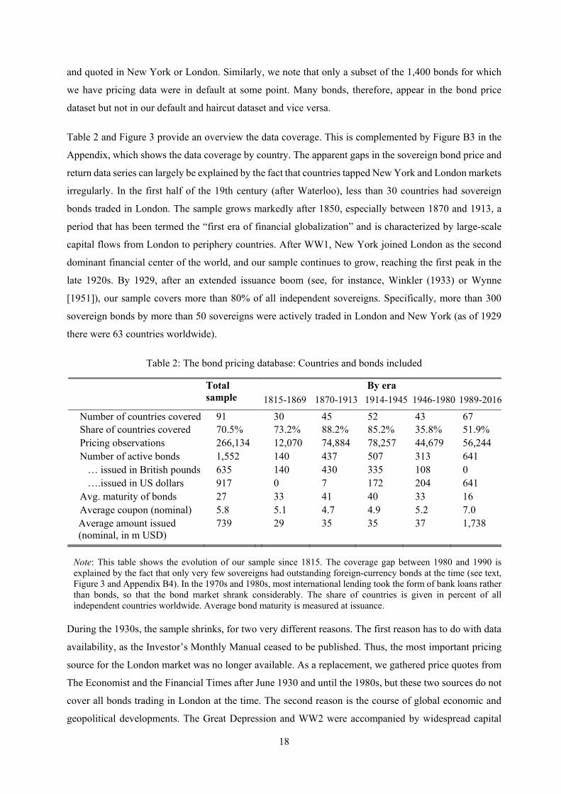
Table 2 and Figure 3 provide an overview the data coverage. This is complemented by Figure B3 in the
Appendix, which shows the data coverage by country. The apparent gaps in the sovereign bond price and
return data series can largely be explained by the fact that countries tapped New York and London markets
irregularly. In the first half of the 19th century (after Waterloo), less than 30 countries had sovereign
bonds traded in London. The sample grows markedly after 1850, especially between 1870 and 1913, a
period that has been termed the “first era of financial globalization” and is characterized by large-scale
capital flows from London to periphery countries. After WW1, New York joined London as the second
dominant financial center of the world, and our sample continues to grow, reaching the first peak in the
late 1920s. By 1929, after an extended issuance boom (see, for instance, Winkler (1933) or Wynne
[1951]), our sample covers more than 80% of all independent sovereigns. Specifically, more than 300
sovereign bonds by more than 50 sovereigns were actively traded in London and New York (as of 1929
there were 63 countries worldwide).
Table 2: The bond pricing database: Countries and bonds included
Total sample
By era 1815-1869 1870-1913 1914-1945 1946-1980 1989-2016
Number of countries covered 91 30 45 52 43 67 Share of countries covered 70.5% 73.2% 88.2% 85.2% 35.8% 51.9% Pricing observations
266,134
12,070 74,884
78,257 44,679 56,244
Number of active bonds 1,552 140 437 507 313 641 … issued in British pounds 635 140 430 335 108 0 ….issued in US dollars 917 0 7 172 204 641 Avg. maturity of bonds
27 33 41 40 33 16
Average coupon (nominal) 5.8 5.1 4.7 4.9 5.2 7.0 Average amount issued (nominal, in m USD)
739 29 35 35 37 1,738
Note: This table shows the evolution of our sample since 1815. The coverage gap between 1980 and 1990 is explained by the fact that only very few sovereigns had outstanding foreign-currency bonds at the time (see text, Figure 3 and Appendix B4). In the 1970s and 1980s, most international lending took the form of bank loans rather than bonds, so that the bond market shrank considerably. The share of countries is given in percent of all independent countries worldwide. Average bond maturity is measured at issuance.
During the 1930s, the sample shrinks, for two very different reasons. The first reason has to do with data
availability, as the Investor’s Monthly Manual ceased to be published. Thus, the most important pricing
source for the London market was no longer available. As a replacement, we gathered price quotes from
The Economist and the Financial Times after June 1930 and until the 1980s, but these two sources do not
cover all bonds trading in London at the time. The second reason is the course of global economic and
geopolitical developments. The Great Depression and WW2 were accompanied by widespread capital

19
account restrictions and a wave of banking crises and sovereign defaults after 1929. These events led to a
sharp decline in cross-border lending worldwide (Reinhart et al. 2018). Moreover, securities of enemy
countries or their allies were banned from trading on the LSE and NYSE after 1939. As a result, the
number of traded bonds with monthly pricing information drops to less than 200.
After 1945, during the era of financial repression and capital controls under the Bretton Woods system,
the sample declines further. 34 This era sees only little international private capital flows and bank lending
overtakes bonds as the preferred vehicle of cross-border lending to sovereigns. As a result, between 1950
and 1990, only 25 countries issued foreign-currency bonds that were actively traded in London and New
York, so our data covers a total of just 117 newly issued sovereign bonds in four decades. While sovereign
bond placements stalled, the 1970s and early 1980s became the era of sovereign syndicated bank lending.
Developing countries borrowed heavily from commercial banks primarily in the United States and
Europe. This lending boom was followed by large-scale defaults on these debts. By the early 1980s, only
a handful of countries still had outstanding bonds at the LSE or NYSE and these instruments were mostly
long-maturity bonds issued in the 1930s and 1940s.
Figure 3: Bond price sample: Coverage across time
Note: The figure shows the coverage of our database by number of bonds (right axis) and countries (left axis, those with at least one active bond), for each year between 1815 and 2016. The sample includes only sovereign bonds issued in USD and GBP and traded in London and/or New York. Both lines are smoothed (5-year moving averages).
Bonds made a comeback only after the developing country debt crisis was resolved. A catalyst was the
Brady Plan of the early 1990s, which involved restructuring deals that securitized the former bank loans.
The newly issued sovereign bonds were traded at a discount. The resulting Brady bonds make up most of
34 See Ilzetzki, Reinhart, and Rogoff (2019) on a global measure of capital controls post 1946.
0
50
100
150
200
250
300
350
400
Act
ive
bond
s
05
1015202530354045505560
Cou
ntrie
s cov
ered
1815 1835 1855 1875 1895 1915 1935 1955 1975 1995 2015
Countries covered (left axis)Active bonds outstanding (right axis)
20
our sample in the 1990s. The reemergence of an active sovereign bond market subsequently encouraged
more and more emerging markets to start issuing foreign-currency bonds in London and New York. By
the early 2000s, bonds had regained their once dominant position in international sovereign lending. As
a result, our sample grows rapidly and reaches a second peak in 2016, with more than 300 foreign-
currency sovereign bonds of 61 countries being actively traded. Further details on the sample and coverage
are shown in Appendix B1.
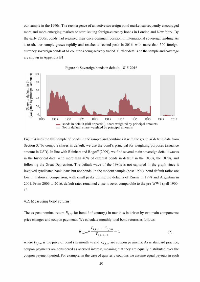
Figure 4: Sovereign bonds in default, 1815-2016
Figure 4 uses the full sample of bonds in the sample and combines it with the granular default data from
Section 3. To compute shares in default, we use the bond’s principal for weighting purposes (issuance
amount in USD). In line with Reinhart and Rogoff (2009), we find several main sovereign default waves
in the historical data, with more than 40% of external bonds in default in the 1830s, the 1870s, and
following the Great Depression. The default wave of the 1980s is not captured in the graph since it
involved syndicated bank loans but not bonds. In the modern sample (post-1994), bond default ratios are
low in historical comparison, with small peaks during the defaults of Russia in 1998 and Argentina in
2001. From 2006 to 2016, default rates remained close to zero, comparable to the pre-WW1 spell 1900-
13.
4.2. Measuring bond returns
The ex-post nominal return 𝑅𝑅𝑖𝑖,𝑗𝑗,𝑡𝑡 for bond i of country j in month m is driven by two main components:
price changes and coupon payments. We calculate monthly total bond returns as follows:
𝑅𝑅𝑖𝑖,𝑗𝑗,𝑚𝑚=𝑁𝑁𝑖𝑖,𝑗𝑗,𝑚𝑚 + 𝐶𝐶𝑖𝑖,𝑗𝑗,𝑚𝑚
𝑁𝑁𝑖𝑖,𝑗𝑗,𝑚𝑚−1− 1 (2)
where 𝑁𝑁𝑖𝑖,𝑗𝑗,𝑚𝑚 is the price of bond 𝑖𝑖 in month 𝑚𝑚 and 𝐶𝐶𝑖𝑖,𝑗𝑗,𝑚𝑚 are coupon payments. As is standard practice,
coupon payments are considered as accrued interest, meaning that they are equally distributed over the
coupon payment period. For example, in the case of quarterly coupons we assume equal payouts in each
0
20
40
60
80
100
Shar
e in
def
ault,
in %
(wei
ghte
d by
prin
cipa
l am
ount
s)
1815 1835 1855 1875 1895 1915 1935 1955 1975 1995 2015Bonds in default (full or partial), share weighted by principal amountsNot in default, share weighted by principal amounts

21
of the three months. To calculate 𝐶𝐶𝑖𝑖,𝑗𝑗,𝑚𝑚, we measure missed or partial coupon payments based on our
newly collected bond-level dataset on default and restructuring outcomes (see Appendix B2). Appendix
B2 also explains how we account for bond haircuts when calculating 𝑁𝑁𝑖𝑖,𝑗𝑗,𝑚𝑚, that is, how we deal with
exchanges of old into new bonds at a loss. In a nutshell, to compute returns in restructuring months, we
combine the old defaulted bonds and the new instruments that creditors receive in the exchange, with the
implicit assumption that creditors keep the newly restructured bond in the portfolio. We then account for
the share of debt written off (face value debt reductions, if any) as well as potential cash payments that
are made in the wake of a restructuring (including for the settlement of past arrears). In case the
restructuring only involves a rescheduling of maturities but no face value debt reduction (sometimes
called “debt reprofiling”), the write-off is zero, while the change in maturities should be reflected in the
secondary market price of the new bond. This also implies that the exact NPV haircut estimation approach
chosen (see Section 3) is not decisive for the computation of the returns series. In fact, the haircut estimate
is a snapshot at one point in time, while returns are measured continuously on a monthly level. Ultimately,
the key default-related variable that matters for the returns is missed coupons, since much of the returns
come from interest payments and if these are not made, total returns drop. We do not account for
transaction fees or taxes (See Appendices B2 and B5 for further details).
We use real ex-post returns as the baseline measure, although we show results for nominal returns as well.
By definition, all bonds in the sample are denominated in GBP or USD, so we need historical inflation
data for the United Kingdom and the United States to compute real returns. For this purpose, we rely on
the historical inflation indices provided by the Bank of England (for GBP bonds) and by the US Bureau
of Labor Statistics (for USD bonds). For a USD bond, the monthly inflation rate is measured as 𝜋𝜋𝑈𝑈𝑈𝑈,𝑚𝑚 =
�𝐶𝐶𝑁𝑁𝐶𝐶𝑈𝑈𝑈𝑈,𝑚𝑚 − 𝐶𝐶𝑁𝑁𝐶𝐶𝑈𝑈𝑈𝑈,𝑚𝑚−1�/𝐶𝐶𝑁𝑁𝐶𝐶𝑈𝑈𝑈𝑈,𝑚𝑚−1, so that the real ex-post return for this USD bond is given by 𝑟𝑟𝑖𝑖,𝑗𝑗,𝑚𝑚 =
𝑅𝑅𝑗𝑗,𝑖𝑖,𝑚𝑚 − 𝜋𝜋𝑈𝑈𝑈𝑈,𝑚𝑚. A comparable process applies to UK bonds. 35
To arrive at yearly global portfolio returns, 36 we compute the monthly weighted global average across
all bonds actively traded in month t.
𝑅𝑅𝑚𝑚𝑝𝑝𝑝𝑝𝑟𝑟𝑡𝑡𝑝𝑝𝑝𝑝𝑝𝑝𝑖𝑖𝑝𝑝=�𝑅𝑅𝑖𝑖,𝑗𝑗,𝑚𝑚
𝑁𝑁
𝑖𝑖=1
∗𝑤𝑤𝑖𝑖,𝑗𝑗,𝑚𝑚
∑ 𝑤𝑤𝑖𝑖,𝑗𝑗,𝑚𝑚𝑁𝑁𝑖𝑖=1
(3)
where 𝑤𝑤𝑖𝑖,𝑗𝑗,𝑚𝑚 denotes the value-weight of bond 𝑖𝑖 of country 𝑗𝑗 for month 𝑚𝑚 and 𝑅𝑅𝑚𝑚𝑝𝑝𝑝𝑝𝑟𝑟𝑡𝑡𝑝𝑝𝑝𝑝𝑝𝑝𝑖𝑖𝑝𝑝 is the realized
return of the global portfolio including bonds 1 to N. In most years, the global portfolio is comprised of a
dominant currency (USD or GBP). The 19th century is dominated by GBP bonds, while the modern post-
1995 sample only includes USD bonds. For some episodes, however, especially during the interwar years,
35 Appendix B5.5 shows that the results are similar when using inflation rates 12 months ahead. 36 Our results are similar when comparing bond prices at the beginning and end of a year (adding all within-year coupon payments) instead of annual averaging.

22
our portfolio contains a mix of USD and GBP bonds. If this is the case, the returns on GBP bonds and
USD bonds enter without converting them into a common currency to avoid bias. This means that, for
those years, we take the perspective of an investor who holds all outstanding foreign-currency bonds
irrespective of whether they are denominated in USD or GBP and who is hedged against currency
fluctuations between these two currencies. 37
In a second step, we compute yearly returns by accumulating monthly returns of month m and year t:
𝑅𝑅𝑡𝑡𝑝𝑝𝑝𝑝𝑟𝑟𝑡𝑡𝑝𝑝𝑝𝑝𝑝𝑝𝑖𝑖𝑝𝑝=��1 + 𝑅𝑅𝑚𝑚
𝑝𝑝𝑝𝑝𝑟𝑟𝑡𝑡𝑝𝑝𝑝𝑝𝑝𝑝𝑖𝑖𝑝𝑝� − 112
𝑚𝑚=1
(4)
To track the return performance over time, we mainly focus on arithmetic averages. This is because
arithmetic returns are the benchmark measure in earlier work on long-run asset performance, for example,
in the EMBI reports or in Dimson, Marsh, and Staunton (2001). For a specific period, say, year 1 through
T, the average portfolio return can be calculated as:
1𝑇𝑇�𝑅𝑅𝑡𝑡
𝑝𝑝𝑝𝑝𝑟𝑟𝑡𝑡𝑝𝑝𝑝𝑝𝑝𝑝𝑖𝑖𝑝𝑝𝑇𝑇
𝑡𝑡=1
(5)
where 𝑅𝑅𝑡𝑡𝑝𝑝𝑝𝑝𝑟𝑟𝑡𝑡𝑝𝑝𝑝𝑝𝑝𝑝𝑖𝑖𝑝𝑝 is the realized return on a given bond portfolio in year t. As an alternative, we also
compute geometric means for each bond and portfolio, meaning the annualized return. 38
Furthermore, as a complement, we also calculate total cumulative returns, which is particularly useful to
assess returns in prespecified event windows (such as around default spells; see Section 5 and Appendix
B8). The formula can be written as ∏ �1 + 𝑅𝑅𝑖𝑖,𝑡𝑡�𝑇𝑇𝑡𝑡=1 − 1 and measures the total return of bond (or portfolio)
i between period 1 and T, where t represents months or years. This formula can also be used to compute
the holding period return, which is the return from holding the investment for a specific period of time.
To compute excess returns, we compare the total returns of each of the bonds in our sample with the
returns on a “risk-free” or safe benchmark in each period. Here, we use total return series on long-term
UK and US government bonds as the benchmark to calculate excess returns. We thus match the total
return of each of the GBP and USD government bonds of a periphery country with the return on long-
term British government gilts or US Treasury bonds at each point in time. More precisely, we calculate
𝑅𝑅𝑁𝑁𝑖𝑖,𝑗𝑗,𝑡𝑡 = 𝑅𝑅𝑖𝑖,𝑗𝑗,𝑡𝑡 − 𝑅𝑅𝑠𝑠𝑠𝑠𝑝𝑝𝑠𝑠,𝑡𝑡, where 𝑅𝑅𝑁𝑁𝑖𝑖,𝑗𝑗,𝑡𝑡 is the excess return of bond i of country j in period t and 𝑅𝑅𝑠𝑠𝑠𝑠𝑝𝑝𝑠𝑠,𝑡𝑡
37 To obtain consistent weights 𝑤𝑤𝑖𝑖,𝑗𝑗,𝑡𝑡 in portfolios with both GBP and USD bonds we convert into USD using the average exchange rates in the year of bond issuance. 38 There can be significant differences between arithmetic and geometric average returns, with arithmetic averages exceeding geometric ones when returns are volatile. Specifically, when returns have a lognormal distribution, the arithmetic return roughly exceeds the geometric return by one-half of the variance. The formula for the geometric
average return for year 1 through T is ∏ �1 + 𝑅𝑅𝑡𝑡𝑝𝑝𝑝𝑝𝑟𝑟𝑡𝑡𝑝𝑝𝑝𝑝𝑝𝑝𝑖𝑖𝑝𝑝�𝑇𝑇
1
1𝑇𝑇 − 1.

23
is the risk-free rate, denominated in the same currency as bond i. Appendix A provides the sources for
these risk-free rates (total return series on UK and US bonds). For completeness, we also compute excess
returns vis-à-vis UK or US bills, which is useful when comparing the risk-return properties of external
sovereign bonds with those of other asset classes (Section 6).
Further methodological details are discussed in Appendixes B2 and B3, including a discussion on how
we deal with historical bond features such as sinking funds.
4.3. Main results on bond returns
Table 3 summarizes our main results. The table shows average yearly sovereign bond returns for our
global portfolio of foreign-currency bonds over 200 years. Henceforth, we do not show returns for the
period 1974 to 1994 due to a lack of representative bond pricing data in the 1970s and 1980s. 39 This
means that the time series for the global portfolio ends in 1973 and starts again in 1995. Appendix B5
shows a number of robustness checks, such as on selection (survivorship) bias and the inflation series
used.
Table 3: Returns on a global portfolio of external sovereign bonds, 1815-2016
Real Return Nominal Return Above US/UK
gov. Bonds
Sharpe ratio
Arithm.
Mean Geom. Mean
SD Arithm. Mean
Geom. Mean
SD
Full sample, 1815-2016, yearly 6.85 5.78 15.03 7.99 7.13 13.69 4.29 0.32 … without world wars 6.99 5.99 14.50 7.69 6.87 13.21 3.94 0.30
By era, yearly 1815-1869 7.10 5.66 17.28 6.90 5.87 14.84 2.96 0.23 1870-1914 6.28 5.97 8.01 6.18 5.91 7.45 3.70 0.48 1915-1945 6.01 4.29 19.91 7.12 6.00 16.19 2.33 0.16 1946-1973 5.85 4.91 14.52 10.15 9.19 15.12 8.07 0.52 1995-2016 9.89 8.96 14.29 12.40 11.41 14.97 6.26 0.33
Monthly returns, full sample 0.54 0.47 3.74 0.65 0.58 3.66 0.35 9.33 Note: Table 3 shows average ex-post investor returns in our total sample of 91 countries and 200 years, as well as for different subsamples. The country composition is changing over time (see Appendix B1). All returns are yearly averages, except for the last line, which shows a monthly frequency. Returns and standard deviations shown are based on a global portfolio that includes all outstanding foreign-currency sovereign bonds at each point in time. Excess returns and Sharpe ratios are computed using US/UK bonds as benchmark.
In the full sample from 1815 to 2016, foreign-currency bonds show an annual ex-post real return of 6.85%,
including spells of turmoil due to defaults, wars, and revolutions. The average is slightly higher (7%)
39 As we explain in Section 3.1. and in Appendix B1, the 1970s and 1980s were a period dominated by syndicated bank lending to sovereigns. Barely any sovereign bonds were issued abroad. As a result, the number of countries with actively traded bonds dropped to fewer than 10 in the 1980s, making the global portfolio unrepresentative.

24
when dropping WW1 and WW2 (1914–18 and 1939–45). Because of the disappearance of new bond
financing in the 1970s and 1980s, this sample omits the encompassing debt crisis in emerging and
developing countries in the 1980s, when commercial bank loans (not bonds) occupied the center stage of
the unfolding default drama. The data that does exist suggests that, during the 1980s, ex-post investor
returns, were well below the historical average (see Appendix B4 for details on the 1970s and 1980s).
Nominal returns exceed real ones in the full sample, but this is driven by the period after WW1. In the
19th century, real returns tend to be higher than nominal returns, due to the many deflationary spells,
including the “Great Deflation” between 1870 and 1890. The geometric total real return is lower, as usual,
with an average of 5.8%. This number represents the annual compounded return of a portfolio that
remained invested for almost two centuries.
Turning to subsamples, the two main eras of financial globalization (1870–1914 and 1995–2016) stand
out. The period 1870–1914 shows an average real annual return of 6.3% per year, coupled with low
volatility (the standard deviation is 8%), while the modern sample shows real annual returns of almost
10%, which is above the historical average. The early 19th century sees high average real returns of about
7%, but also a high return volatility. The interwar years, with an exceptionally high incidence of defaults,
show the worst risk-return ratio, with lower-than-average real returns of 6.01% (the geometric return is
just 4.3%) and a standard deviation of 19.9%. The returns are lowest in the three decades following WW2,
mostly due to the fact that many bonds that went into default in the 1930s continued to be nonperforming
for decades. It took until the 1980s to settle all the defaults of the 1930s and 1940s, with a total of 41
restructurings. 40 At the same time, barely any bond issuances occurred, so that the averages for this era
are biased downward due to selection effects.
Since our sample is unbalanced, we explore the issue of survival bias and sample composition in Appendix
B5.1, by focusing on 15 countries for which we have more than 100 years of data each, resulting in a
more balanced sample. The returns for these 15 countries are similar to our baseline numbers that build
on all 91 countries, some of which only have data for a few years. This alleviates concerns that our main
finding is biased due to sample issues.
The observed returns can mainly be attributed to coupon payments (gains from interest) rather than price
changes (capital gains). Around 70%, or 5.6 percentage points, of the nominal yearly return of 8.0% over
the past 200 years is due to coupon payments. Coupons are the main driver of returns in each decade,
roughly contributing between 4 and 8 percentage points to the ex-post nominal returns. Appendix B5.2.
provides further details on coupon versus price effects.
40 At the end of World War 2, there were still only 69 sovereign nations.

25
Figure 5 explores the distribution of returns in our global bond portfolio. We examine the distribution
because the standard deviation can understate the degree of risk due to a skewed distribution with fat tails.
The return distribution does not look overly skewed. Despite some positive and negative outliers, the plot
for the full sample (Panel A) is roughly in line with a normal distribution (which is also true for the
monthly data). We nevertheless compute adjusted Sharpe ratios, to account for volatility, skewness, and
kurtosis (the differences are small; see, for example, Section 6).
Figure 5: Distribution of bond returns and bond prices, 1815-2016
Panel A: Bond returns - full sample Panel B: Bond returns - (real, arithmetic average total returns) default vs non-default spells
Panel C: Bond prices – default vs non-default spells
Notes: This upper part of this figure shows the distribution of yearly real returns. Panel A uses aggregate yearly returns based on the global sovereign bond portfolio. Panel B uses bond-level data and distinguishes between years in default and non-default years. Panel C shows the distribution of bond prices as reported in the primary sources (mixing USD and British Pound prices) for default and non-default years and also using bond-level data.
In default years (Panel B), the distribution differs markedly, with a lower average real return and much
fatter tails. However, the coefficient for skewness remains close to zero, suggesting that years of investor
losses and years of recoveries balance each other out in normal times and in crisis times (see also Section
4 on bond performance following a default). Furthermore, Panel C shows that there is much more skew
Mean: 6.85Median: 6.58Scewness: 0.26
0
3
5
8
10
13
15
Perc
ent
-40 -20 0 20 40 60
Total returns (yearly, real, arithmetic avg.)normal distribution
Non-default years:Mean: 6.05Median: 4.85Skewness: 1.09 Default years:Mean: 2.37Median: 1.98Skewness: 0.17
0
5
10
15
20
25
30
Perc
ent
-100 0 100Total returns (yearly, real, arithmetic avg.)
Non-default years Default years
Non-default years:Mean: 88.47Median: 95.00Skewness: -1.14 Default years:Mean: 35.09Median: 25.00Skewness: 0.97
0
5
10
15
20
Perc
ent
0 50 100 150Bond prices (end of year)
Non-default years Default years

26
when looking at bond prices only. During default, the average bond price is just 35 USD or GBP, with a
strong left skew. In non-default years the average price is 89 and the distribution has a right skew.
To allow for different investment horizons, we next turn to holding period returns (HPRs). Table 4 shows
average HPRs across years and countries (for completeness, we start on a quarterly basis). After 10 years,
the mean HPR in our full sample is 94%, with a median of 84.7%. The upper bucket (75th percentile)
shows a 126.5% real return over 10 years, while the lower bucket (25th percentile) shows a cumulative
return of 59.5%. We also show geometric and arithmetic means per year. Over time, the geometric mean
decreases due to the occurrence of defaults. In contrast, the returns using arithmetic averaging remain in
the range of 6 to 7% per year.
Table 4: Holding period returns on a global portfolio of external sovereign bonds, 1815-2016
Note: This table shows holding periods ranging from Q1 to year 10. The average geometric mean is reported for quarterly holding periods on a quarterly basis, that is, it gives the average, real compounded return for one quarter. For the annual holding periods, the geometric mean states the average, annualized return for the specific holding period. All return statistics are based on a global portfolio of outstanding foreign-currency sovereign bonds.
Figure 6 zooms in on the subsample of the worst-performing bonds, in which the repudiation cases figure
prominently. We calculate the share of bonds with negative real compounded returns after different
holding periods. In the full sample, in year one, more than 26% of the observations see negative returns,
and this drops to below 20% in year 10 (Panel A). Moreover, there are about 10% of observations with
substantial losses, showing a negative return of -30% or worse, as well as a small but growing share of
bonds with returns between -30% and -60%. Observations in this bottom bin are dominated by spells after
the Great Depression and around WW2, for example, in many Communist countries (China, Russia, and
Eastern Europe), which saw a large initial collapse in bond prices and defaults that persisted for decades.
In the modern (post-1995) period, the share of bonds with negative returns is much lower than in the
historical sample (Panel B), partially reflecting the relative absence of full repudiation cases. After three
years, only about 7% of the country observations remain in negative territory. The share with very low
Quarterly (Q1-Q4) Yearly (years 1-10) Q1 Q2 Q3 Q4 1 2 3 4 5 6 7 8 9 10
Mean (arithmetic, cumulative) 2.7 3.9 5.3 6.8 6.8 14.7 22.9 31.3 40.8 50.3 60.3 70.8 81.8 94
p75 6.3 8.6 12.6 14.4 14.4 27.3 41 55.8 64.7 77.4 85.3 100.1 110.6 126.5 Median 2.7 3.9 4.4 6.6 6.6 12.4 18 25.6 32.3 40.9 51.3 61.7 71.5 84.7 p25 -0.3 -1.2 -1.5 -1.5 -1.5 1.8 3.7 6.1 14.5 21.5 31.2 39.8 48.5 59.5
Mean (arithmetic, avg. per period) 2.7 2 1.8 1.7 6.8 6.9 6.9 7 7.1 7.2 7.4 7.4 7.4 7.5 Mean (geometric, annualized) 2.7 1.8 1.6 1.5 6.8 6.5 6.3 6.2 6.3 6.3 6.4 6.5 6.5 6.5
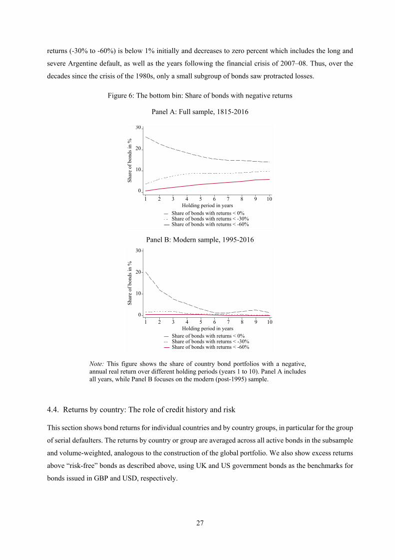
27
returns (-30% to -60%) is below 1% initially and decreases to zero percent which includes the long and
severe Argentine default, as well as the years following the financial crisis of 2007–08. Thus, over the
decades since the crisis of the 1980s, only a small subgroup of bonds saw protracted losses.
Figure 6: The bottom bin: Share of bonds with negative returns
Panel A: Full sample, 1815-2016
Panel B: Modern sample, 1995-2016
Note: This figure shows the share of country bond portfolios with a negative, annual real return over different holding periods (years 1 to 10). Panel A includes all years, while Panel B focuses on the modern (post-1995) sample.
4.4. Returns by country: The role of credit history and risk
This section shows bond returns for individual countries and by country groups, in particular for the group
of serial defaulters. The returns by country or group are averaged across all active bonds in the subsample
and volume-weighted, analogous to the construction of the global portfolio. We also show excess returns
above “risk-free” bonds as described above, using UK and US government bonds as the benchmarks for
bonds issued in GBP and USD, respectively.
0
10
20
30Sh
are
of b
onds
in %
1 2 3 4 5 6 7 8 9 10Holding period in years
Share of bonds with returns < 0%Share of bonds with returns < -30%Share of bonds with returns < -60%
0
10
20
30
Shar
e of
bon
ds in
%
1 2 3 4 5 6 7 8 9 10Holding period in years
Share of bonds with returns < 0%Share of bonds with returns < -30%Share of bonds with returns < -60%

28
We start with a group of 51 “serial defaulters.” These are countries that have defaulted on their external
debt at least twice since 1815 (or independence). 41 Appendix B5.4 shows that the results are similar when
using a stricter definition of serial defaulters, that is, for countries with at least three or at least four
defaults. The second group of 40 countries (“Others”) includes non-defaulters and one-time defaulters. 42
The default data are from Reinhart and Rogoff (2009), updated by Reinhart and Trebesch (2016) and here.
Table 5: Bond returns by country group and era
Arithmetic mean
(annual)
Geometric mean
(annual)
SD Excess return (mean, above
UK/US bonds)
Total Sample (1815-2016) Serial defaulters 7.1 5.8 16.8 4.6 Other countries with ext. bonds 5.6 5.1 10.4 3.4 UK/US government bonds 2.9 2.5 9.3
Early 19th Century (1815-1869) Serial defaulters 7.0 5.5 17.8 2.9 Other countries with ext. bonds 5.8 5.4 10.1 1.8 UK government bonds 5.1 4.6 10.2
Pre-WW1 (1870-1913) Serial defaulters 6.6 6.2 9.4 4.1 Other countries with ext. bonds 5.3 5.2 4.0 2.6 UK government bonds 2.5 2.5 3.9
Interwar (1920-1937) Serial defaulters 6.8 4.8 21.2 -2.8 Other countries with ext. bonds 10.5 9.4 16.5 1.0 US government bonds 6.5 5.9 11.5 Today (1995-2016) Serial defaulters 9.9 9.0 14.5 6.3 Other countries with ext. bonds 7.4 7.1 9.3 4.9
US government bonds 4.0 3.7 8.2
Notes: This table shows summary statistics of yearly total real returns on foreign-currency sovereign bonds across 200 years for different country groups. Serial defaulters had two or more external defaults or were in default for a very long time (their share of years in default since independence is above the sample median of 20%). Other countries are those that never defaulted or only for a brief period (share of years in default below the median). Excess returns above UK/US bonds are computed at the bond level.
Table 5 shows summary statistics for the three groups, (i) serial defaulters, (ii) “other” sovereigns that
issued debt in USD and GBP abroad, and (iii) “risk-free” US or UK long-term government bonds. The
41 Specifically, the group includes Argentina, Austria/Austria-Hungary, Belize, Bolivia, Brazil, Bulgaria, Chile, China, Colombia, Costa Rica, Cote d'Ivoire, Cuba, Czech Republic/Czechoslovakia, Dominican Republic, Ecuador, Egypt, El Salvador, Gabon, Germany, Ghana, Greece, Guatemala, Haiti, Honduras, Hungary, Indonesia, Jamaica, Kazakhstan, Mexico, Morocco, Nicaragua, Nigeria, Pakistan, Panama, Paraguay, Peru, Philippines, Poland, Portugal, Romania, Russia, Senegal, Serbia/ Yugoslavia, South Africa, Spain, Sri Lanka, Turkey/Ottoman Empire, Ukraine, Uruguay, Venezuela, and Zimbabwe. 42 Algeria, Angola, Armenia, Australia, Azerbaijan, Belarus, Belgium, Cameroon, Canada, Croatia, Denmark, Estonia, Ethiopia, Finland, France, Georgia, Iraq, Ireland, Italy, Japan, Jordan, Kenya, Latvia, Lebanon, Lithuania, Malaysia, Mongolia, Namibia, Netherlands, New Zealand, Norway, Slovak Republic, South Korea, Sweden, Switzerland, Tanzania, Thailand, Trinidad and Tobago, Vietnam, Zambia.
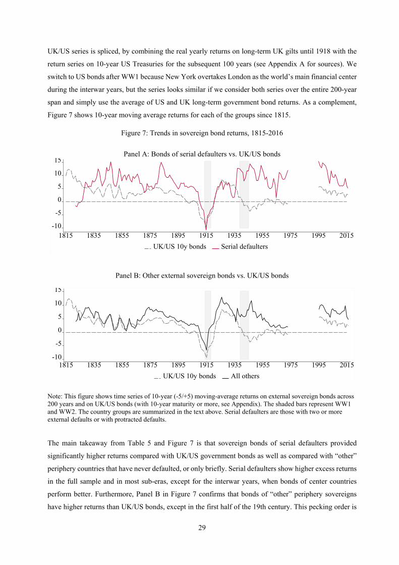
29
UK/US series is spliced, by combining the real yearly returns on long-term UK gilts until 1918 with the
return series on 10-year US Treasuries for the subsequent 100 years (see Appendix A for sources). We
switch to US bonds after WW1 because New York overtakes London as the world’s main financial center
during the interwar years, but the series looks similar if we consider both series over the entire 200-year
span and simply use the average of US and UK long-term government bond returns. As a complement,
Figure 7 shows 10-year moving average returns for each of the groups since 1815.
Figure 7: Trends in sovereign bond returns, 1815-2016
Panel A: Bonds of serial defaulters vs. UK/US bonds
Panel B: Other external sovereign bonds vs. UK/US bonds
Note: This figure shows time series of 10-year (-5/+5) moving-average returns on external sovereign bonds across 200 years and on UK/US bonds (with 10-year maturity or more, see Appendix). The shaded bars represent WW1 and WW2. The country groups are summarized in the text above. Serial defaulters are those with two or more external defaults or with protracted defaults. The main takeaway from Table 5 and Figure 7 is that sovereign bonds of serial defaulters provided
significantly higher returns compared with UK/US government bonds as well as compared with “other”
periphery countries that have never defaulted, or only briefly. Serial defaulters show higher excess returns
in the full sample and in most sub-eras, except for the interwar years, when bonds of center countries
perform better. Furthermore, Panel B in Figure 7 confirms that bonds of “other” periphery sovereigns
have higher returns than UK/US bonds, except in the first half of the 19th century. This pecking order is
-10
-5
0
5
10
15
1815 1835 1855 1875 1895 1915 1935 1955 1975 1995 2015UK/US 10y bonds Serial defaulters
-10
-5
0
5
10
15
1815 1835 1855 1875 1895 1915 1935 1955 1975 1995 2015UK/US 10y bonds All others
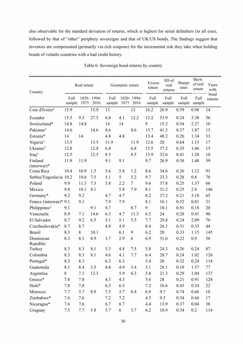
30
also observable for the standard deviation of returns, which is highest for serial defaulters (in all eras),
followed by that of “other” periphery sovereigns and that of UK/US bonds. The findings suggest that
investors are compensated (primarily via rich coupons) for the incremental risk they take when holding
bonds of volatile countries with a bad credit history.
Table 6: Sovereign bond returns by country
Country Real return Geometric return Excess
return
SD of real
returns
Sharpe ratio
Skew. of real return
Years with bond
returns Full sample
1820-1973
1994-2016 Full
sample 1820-1973
1994-2016 Full
sample Full
sample Full
sample Full
sample
Cote d'Ivoire° 15.9 15.9 13 13 16.2 26.9 0.59 0.98 14
Ecuador 15.5 9.3 27.5 6.8 4.1 12.2 13.2 53.9 0.24 3.38 56 Switzerland* 14.8 14.8 14 14 9 15.2 0.54 2.27 10 Pakistan° 14.6 14.6 8.6 8.6 15.7 41.5 0.37 1.87 13 Estonia* 14 14 4.8 4.8 13.4 48.2 0.26 1.34 33 Nigeria° 13.5 13.5 11.9 11.9 12.6 20 0.64 1.13 17 Ukraine° 12.8 12.8 6.8 6.8 13.5 37.2 0.35 1.06 15 Iraq° 12.5 12.5 8.5 8.5 13.9 32.6 0.41 1.28 10 Finland (interwar)*
11.9 11.9 9.1 9.1 9.7 26.9 0.38 1.48 39
Costa Rica 10.4 10.9 1.5 5.6 5.8 1.2 8.6 34.6 0.26 1.12 91 Serbia/Yugoslavia 10.2 10.6 7.5 5.1 5 5.2 9.7 33.3 0.28 0.8 70 Poland 9.9 11.3 7.3 3.8 2.2 7 9.6 37.8 0.25 1.57 66 Mexico 9.8 10.1 8.1 5.8 7.9 8.1 31.2 0.25 2.8 146 Germany* 9.2 9.2 4.7 4.7 8.2 37.2 0.21 3.18 65 France (interwar)* 9.1 9.1 7.9 7.9 8.1 16.1 0.52 0.01 31 Philippines° 9.1 9.1 8.7 8.7 9 10.1 0.91 0.18 20 Venezuela 8.9 7.1 14.6 6.3 4.7 11.3 6.5 24 0.28 0.41 90 El Salvador 8.7 9.2 6.5 5.1 5.1 5.5 7.7 29.8 0.24 2.09 70 Czechoslovakia* 8.7 8.7 4.9 4.9 8.4 26.1 0.31 0.33 44 Brazil 8.3 8 10.1 6.1 9 6.2 20 0.33 1.15 145 Dominican Republic
8.3 8.1 8.9 3.7 2.9 6 6.9 31.6 0.22 0.9 56
Turkey 8.3 8.3 8.1 5.3 4.8 7.5 5.8 24.3 0.26 0.24 87 Colombia 8.3 8.3 8.1 4.6 4.1 7.7 6.4 28.7 0.24 1.02 126 Portugal* 8.3 8.3 6.3 6.3 5.4 20 0.32 0.24 114 Guatemala 8.1 8.4 3.5 4.8 4.9 3.4 5.1 28.1 0.19 1.57 77 Argentina 8 7.3 12.3 5.9 6.3 5.8 21.3 0.29 1.04 137 Greece* 7.8 7.8 4.3 4.3 5.6 28 0.21 0.91 128 Haiti* 7.8 7.8 6.5 6.5 7.2 16.6 0.45 0.24 22 Morocco 7.7 3.7 8.9 7.3 3.7 8.4 6.9 9.7 0.74 0.66 18 Zimbabwe* 7.6 7.6 7.2 7.2 4.5 9.5 0.54 0.66 17 Nicaragua* 7.6 7.6 6.7 6.7 4.4 13.9 0.37 0.04 38 Uruguay 7.5 7.7 5.8 5.7 6 3.7 6.2 18.9 0.34 0.2 114

31
Japan* 7.4 7.4 5.9 5.9 5.6 19.9 0.29 2.82 99 Lebanon° 7.3 7.3 7.1 7.1 7.9 6.8 1.04 1.66 16 Panama 7.2 7.4 7.1 6.1 5.6 6.8 7.2 14.6 0.47 -0.67 46 Cuba* 7.1 7.1 5.8 5.8 6.2 17.2 0.38 1.35 72 Chile 7 7.3 4.3 4.8 4.9 4.2 5.1 20.5 0.26 0.71 150 Paraguay 6.9 7 5 2 1.9 4.9 3.7 34.6 0.11 1.64 57 Italy* 6.9 6.9 3.9 3.9 4.2 22.2 0.21 1.3 103 Netherlands* 6.5 6.5 6.4 6.4 3.1 5.1 0.88 -0.17 25 Indonesia° 6.4 6.4 5.6 5.6 7.3 13.6 0.51 0.69 12 Egypt 6.2 6.4 5.2 5.5 5.6 4.8 4.1 12.8 0.41 0.52 93 Sweden (pre-WW2)*
6.1 6.1 5.3 5.3 2.7 13.7 0.32 3.26 66
Spain* 6 6 3.6 3.6 3.7 23.4 0.17 2.02 131 Bulgaria 6 4.6 10.9 0.8 -1.6 10 5.3 34.8 0.16 1.42 88 Hungary 5.8 5.9 5 2.7 2.5 4.6 4.6 26.1 0.18 1.36 107 Croatia° 5.7 5.7 5.4 5.4 6.2 8.6 0.74 1.27 11 Honduras 5.6 5.4 11.2 0.9 0.5 11.1 3 30.2 0.1 0.3 71 Russia 5.6 4.4 13.9 0.6 0.1 3.8 3.4 34.9 0.1 3.11 150 Denmark* 5.5 5.5 4.2 4.2 3.7 17.6 0.23 1.56 92 Malaysia° 5.2 5.2 5.2 5.2 4.9 4.5 1.06 0.64 10 Belgium* 5.2 5.2 4.1 4.1 4 16.2 0.25 2.45 83 Vietnam° 5.2 5.2 4.7 4.7 6.1 10.6 0.53 0.35 11 Peru 4.8 4.2 8.1 1.8 0.8 7.6 3.4 25.2 0.14 0.68 124 Norway* 4.6 4.6 3.7 3.7 3 14.7 0.22 1.46 93 Romania 4.4 16.8 3.2 3.8 3.8 3.1 14.8 79.6 0.18 4.88 78 Thailand 4.4 4.3 5.5 3.5 3.3 5.4 2.8 14.5 0.3 1.88 51 South Africa 4.3 3.9 5.7 3.8 3.4 5.4 2.6 10.4 0.39 1.5 89 Austria* 3.9 3.9 0.5 0.5 4.7 25.8 0.19 0.45 41 Ireland* 3.8 3.8 3.2 3.2 2.6 10.4 0.32 0.14 24 New Zealand* 3.7 3.7 3.3 3.3 1.6 9.8 0.29 1.7 93 Australia* 3.6 3.6 3 3 2 12 0.2 2.17 101 Canada* 3.1 3.1 2.7 2.7 1.5 9.3 0.3 1.71 96 Bolivia 2.5 1.5 7.3 -3.3 -5.3 7.2 -0.2 28.6 -0.01 -0.87 24 China 2.1 1.8 4.3 -1.1 -1.8 4.2 0.8 26.7 0.03 2.4 103 Cross-country average 7.7 7.2 8.6 5.1 4.2 6.8 6.4 23.2 0.35 1.26 68 Cross-country median 7.4 7.3 7.4 5 4.5 6.6 5.8 21.3 0.29 1.15 70
Notes: The table shows average annual real ex-post returns by country, using arithmetic averages across all bonds outstanding at each point in time (country portfolios). Only countries with 10 or more years of data are included. For countries marked with (*) we only have historical bond returns (in the sample 1815-1973). This applies to many of today’s advanced economies which have stopped issuing external sovereign bonds in London or New York and borrow domestically instead. For countries marked with a circle (°) we only have returns in the modern sample (1995-2016). See Appendix B1 for a detailed overview of the years covered by country and on how we deal with country break-ups and country mergers when splicing the long-run country series (e.g., Austria-Hungary, Ottoman Empire, Prussia-Germany).
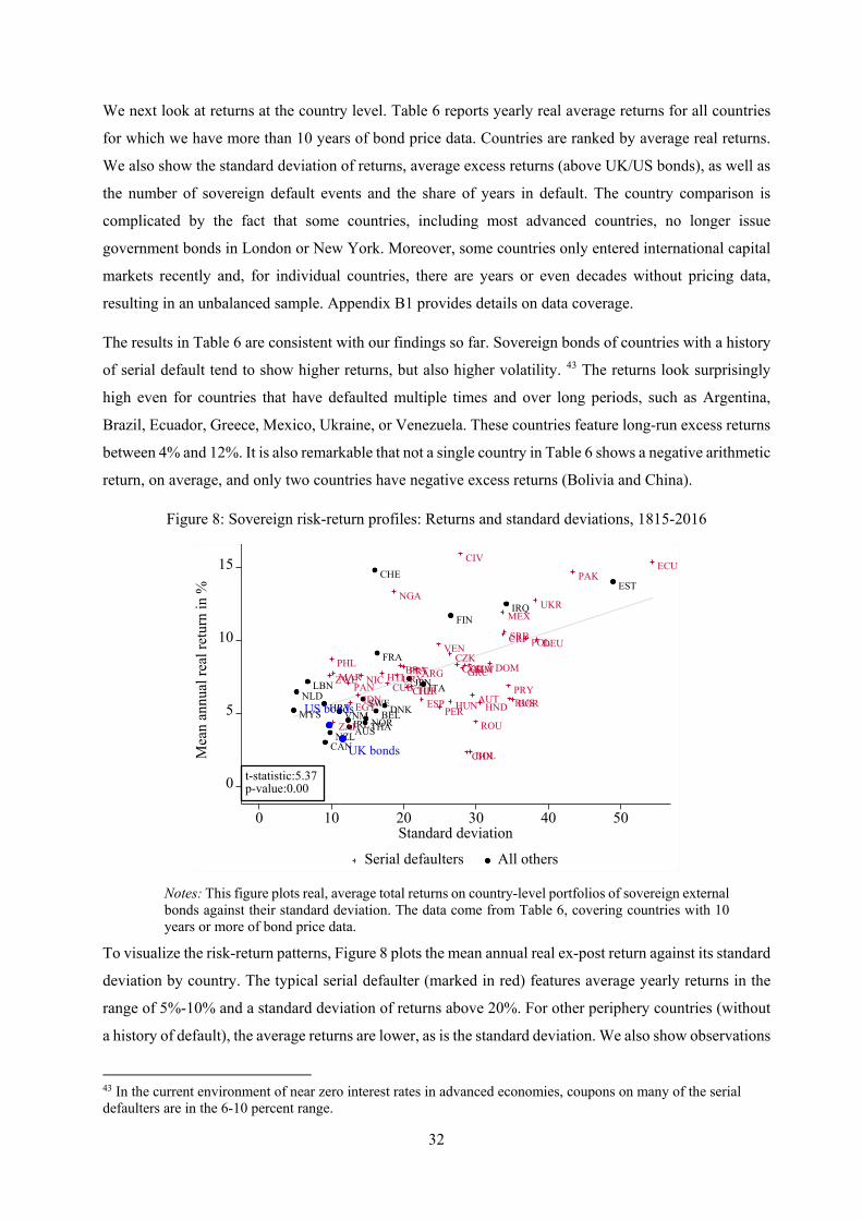
32
We next look at returns at the country level. Table 6 reports yearly real average returns for all countries
for which we have more than 10 years of bond price data. Countries are ranked by average real returns.
We also show the standard deviation of returns, average excess returns (above UK/US bonds), as well as
the number of sovereign default events and the share of years in default. The country comparison is
complicated by the fact that some countries, including most advanced countries, no longer issue
government bonds in London or New York. Moreover, some countries only entered international capital
markets recently and, for individual countries, there are years or even decades without pricing data,
resulting in an unbalanced sample. Appendix B1 provides details on data coverage.
The results in Table 6 are consistent with our findings so far. Sovereign bonds of countries with a history
of serial default tend to show higher returns, but also higher volatility. 43 The returns look surprisingly
high even for countries that have defaulted multiple times and over long periods, such as Argentina,
Brazil, Ecuador, Greece, Mexico, Ukraine, or Venezuela. These countries feature long-run excess returns
between 4% and 12%. It is also remarkable that not a single country in Table 6 shows a negative arithmetic
return, on average, and only two countries have negative excess returns (Bolivia and China).
Figure 8: Sovereign risk-return profiles: Returns and standard deviations, 1815-2016
Notes: This figure plots real, average total returns on country-level portfolios of sovereign external bonds against their standard deviation. The data come from Table 6, covering countries with 10 years or more of bond price data.
To visualize the risk-return patterns, Figure 8 plots the mean annual real ex-post return against its standard
deviation by country. The typical serial defaulter (marked in red) features average yearly returns in the
range of 5%-10% and a standard deviation of returns above 20%. For other periphery countries (without
a history of default), the average returns are lower, as is the standard deviation. We also show observations
43 In the current environment of near zero interest rates in advanced economies, coupons on many of the serial defaulters are in the 6-10 percent range.
AUSBEL
CAN
HRV DNK
EST
FIN
FRA
IRQ
IRL
ITAJPNLBN
MYS
NLD
NZLNOR
SWE
CHE
THAVNM
ARG
AUT
BOL
BRA
BGRCHL
CHN
COL
CRI
CIV
CUB
CZKDOM
ECU
EGY
SLV
DEU
GRCGTMHTI
HNDHUNIDN
MEX
MAR NIC
NGA
PAK
PAN PRY
PER
PHL
POL
PRT
ROU
RUS
ZAF
ESPTUR
UKR
URY
VENSRB
ZWE
UK bonds
US bonds
t-statistic:5.37p-value:0.000
5
10
15
Mea
n an
nual
real
retu
rn in
%
0 10 20 30 40 50Standard deviation
Serial defaulters All others

33
for “risk-free” UK and US government bonds (marked in blue) using the full 200-year series for both
countries (the average yearly real return is 3.4% for US bonds and 4.1% for UK bonds, with standard
deviations of 12% and 10%, respectively).
Figure 9 focuses on country credit histories and plots the average yearly real ex-post bond returns on the
vertical axis against the total number of external sovereign default events (on private external debt) since
1815 on the horizontal axis, using the updated Reinhart and Rogoff (2009) default data. Similar to Figure
7, we find that bond returns increase in the riskiness of a country, as measured by the number of past
defaults. In Appendix B7, we add to these results with a capital asset pricing model (CAPM) analysis.
Serial defaulters have higher betas, as bond returns for these countries are more sensitive to US/UK stock
market conditions.
Figure 9: The role of credit history: Returns and default frequency, by country, 1815-2016
Notes: This figure plots real, average total returns on country-level portfolios of sovereign external bonds against the total number of defaults since independence by that country on the horizontal axis. The data come from Table 6, covering countries with 10 years or more of bond price data. The default data from Reinhart and Rogoff (2009) and updated in Reinhart and Trebesch (2016).
4.5. Liquidity of the sovereign bond market over the past 200 years
This section gives a brief overview on sovereign bond market liquidity over 200 years, as proxied by bid-
ask spreads (additional insights are provided in Appendix B6). To complement our main database of
prices, haircuts and returns, we gathered a large additional dataset of bid and ask bond prices. The resulting
bid-ask spread series cover all countries in our sample, but with some gaps, in particular in the first half
of the 19th century (see Figure B3). In total, we could gather monthly, bond-level bid-ask spreads for 62%
of our pricing sample (165,638 out of 266,134 observations). For historical bonds traded on the London
AUS
BEL
CAN
HRVDNK
EST
FIN
FRA
IRQ
IRL
ITAJPNLBN
MYS
NLD
NZLNOR
SWE
CHE
THAVNM
ARG
AUT
BOL
BRA
BGRCHL
CHN
COL
CRI
CIV
CUB
CZKDOM
ECU
EGY
SLV
DEU
GRC GTMHTI
HNDHUN IDN
MEX
MAR NIC
NGA
PAK
PAN PRY
PER
PHL
POL
PRT
ROU
RUS
ZAF
ESP
UKR
URY
VENSRB
ZWE
TUR
UK bonds
US bonds
t-statistic:1.87p-value:0.070
5
10
15
Mea
n an
nual
real
retu
rn in
%
0 1 2 3 4 5 6 7 8 9 10 11Number of external defaults
Serial defaulters All others

34
Stock Exchange, we follow Alquist (2010) and Chavaz and Flandreau (2017) and use the spread between
the so-called “business done” and the “closing price” as a proxy for bid-ask spreads (71,108 observations).
Using these data, we compute 𝑠𝑠𝑠𝑠𝑟𝑟𝑠𝑠𝑠𝑠𝑠𝑠𝑖𝑖,𝑡𝑡 =𝑃𝑃𝑖𝑖,𝑡𝑡𝐴𝐴𝐴𝐴𝐴𝐴−𝑃𝑃𝑖𝑖,𝑡𝑡
𝐵𝐵𝑖𝑖𝐵𝐵
12�𝑃𝑃𝑖𝑖,𝑡𝑡
𝐴𝐴𝐴𝐴𝐴𝐴+𝑃𝑃𝑖𝑖,𝑡𝑡𝐵𝐵𝑖𝑖𝐵𝐵�
, which represents the spread of bid and ask prices,
𝑁𝑁𝑖𝑖,𝑡𝑡𝐵𝐵𝑖𝑖𝐵𝐵 and 𝑁𝑁𝑖𝑖,𝑡𝑡𝐴𝐴𝑠𝑠𝐴𝐴, of bond i in month t. We then compute an aggregate proxy for market liquidity by
averaging the time series of bond-level, bid-ask spreads in our global portfolio on a monthly level as
follows: 𝑀𝑀𝑠𝑠𝑟𝑟𝑀𝑀𝑠𝑠𝑡𝑡𝑀𝑀𝑖𝑖𝑀𝑀𝑀𝑀𝑖𝑖𝑠𝑠𝑖𝑖𝑡𝑡𝑀𝑀𝑡𝑡 = 1𝑁𝑁𝑡𝑡∑ 𝑠𝑠𝑠𝑠𝑟𝑟𝑠𝑠𝑠𝑠𝑠𝑠𝑖𝑖,𝑡𝑡𝑁𝑁𝑡𝑡𝑖𝑖=1 , where 𝑁𝑁𝑡𝑡 is the number of bonds i trading in month t. 44
Figure 10: Bid-ask spreads and total returns, 1870-2016
Panel A: 1870-1970
Panel B: 1995-2016
Note: This graph shows monthly bid-ask spreads (blue line) and total real returns (red shaded) for the global external bond portfolio. Both series are computed as 12-month moving-average (-6/+6). The shaded grey bars represent major crises, wars, and global shocks.
Figure 10 shows a 200-year time series of monthly bid-ask spreads and total returns for our global bond
portfolio, with two key insights. First, the figure suggests that the liquidity of this asset class may
importantly depend on global events, often originating or affecting the financial centers. Average bond
liquidity declines markedly during global wars and financial crises, with bid-ask spreads spiking in the
44 The graph looks very similar when using weighted average bid-ask spreads (e.g. weighted by issuance amounts).
Panicof 1907
Viennacrash
WorldWar I
WorldWar II
GreatDrepression
Panicof 1873
Egyptand
Ottoman Empiredefault
Baringcrisisand
defaultArgentina
Russiandefault,Empire
break-ups
-5
0
5
10
1870 1875 1880 1885 1890 1895 1900 1905 1910 1915 1920 1925 1930 1935 1940 1945 1950 1955 1960 1965 1970
Total real returns (monthly moving average, in %) Bid-ask spreads (monthly moving average, in %)
Russiadefault
andLTCM crisis
Argentina defaults,Brazil crisis
Lehmannbankruptcy
Asian crisis
Greekrestructuring
announcement
-5
0
5
1995 1996 1997 1998 1999 2000 2001 2002 2003 2004 2005 2006 2007 2008 2009 2010 2011 2012 2013 2014 2015 2016
Total real returns (monthly moving average, in %) Bid-ask spreads (monthly moving average, in %)

35
initial months of the shock. WW2 had a particularly lasting impact, as market liquidity never fully
recovered after 1945, with average bid-ask spreads remaining at a level far above those in the 1920s. Also,
idiosyncratic crises affected aggregate market liquidity, for example the Ottoman and Egyptian defaults
in the 1870s, the Russian default in 1998, or the Argentine defaults in the 1890s and early 2000s.
Second, total returns tend to be higher when bid-ask spreads are high, except for the first months of major
shocks, when returns collapse while bid-ask spreads spike. On average, higher risk is associated with
lower market liquidity. Appendix B6 confirms this using bond-level data, as average returns are
significantly higher for less liquid bonds. The difference between the most liquid and least liquid bonds
is large and statistically significant, especially in the historical sample, which is in line with Alquist (2010)
and Chavaz and Flandreau (2017), who also find a substantial sovereign bond liquidity premium. An in-
depth analysis of sovereign bond market liquidity over the full 200 years is left for future research.
5. Investor performance around debt crises: Returns, defaults, and haircuts
This section studies the link between bond returns, defaults, and haircuts, by combining the data on debt
restructurings and creditor losses from Section 3 with those on bond prices and returns from Section 4.
Figure 11: Bond returns around sovereign defaults
Note: This figure shows total cumulative returns on sovereign external bonds around default events, using real, monthly return data and taking into account losses due to missed coupons and haircuts. The total return series are normalized to one in year two (24 months) prior to the default. The bold black line shows the average across all defaulted bonds, while the dotted grey lines show upper and lower quartiles. We include all 92 default episodes for which we have sufficient pricing data before and after the default.
Figure 11 shows a time series of total returns around all the sovereign bond default events in our sample
for which we have sufficient bond price data, in the run-up and the aftermath of default. These are 92
cases of a total of 161 sovereign bond defaults in the sample. (This exercise does not include the many
defaults on bank loans for which no prices exist; see Figure 1.) The total cumulative return series is
Averagecumulative
return
Upper 75%
Lower 25%
50
75
100
125
150
175
Cum
ulat
ive
tota
l ret
urn
inde
x
-2 -1 t 1 2 3 4 5 6Years around default
Start of holding period: 2 years before default

36
indexed to two years (24 months) prior to the default. The bold black line shows the average across all
bonds in the global portfolio, while the dotted grey lines show the upper and lower quartiles.
Figure 12: Returns around default: High vs. low haircut cases
As expected, sovereign bonds perform badly in the wake of a default event. The total cumulative return
drops by about 15% initially and then stagnates for a few years, as debt crises tend to linger for nearly
eight years, on average (Reinhart and Rogoff 2009). Investors who enter two years pre-default break even
four years after the initial default date, on average, thus recouping the losses suffered with delay (this can
be described as a U-shaped recovery). However, the variation is large. About 25% of all defaults (upper
quartile) see barely any drop in total returns and investors increase their invested capital by 50% five years
after the default, on average. In contrast, cases in the bottom 25% (lower quartile) do not show a recovery;
the pattern is L-shaped, as six years after the first default, investors are still in negative territory, far from
breaking even. Almost all the defaults in the bottom quartile occur in the historical (pre-WW2) period,
including defaults that took decades to settle. Since the 1990s, only the bond defaults of Argentina in 2001
and Ecuador in 2008 produced long-lasting creditor losses. Specifically, it took investors until 2016 to
break even in Argentina (15 years) and about five years after Ecuador’s 2008 default. We also check
holding period returns around default, using geometric instead of arithmetic average returns. The
takeaway is similar to that in Figure 10, as investors entering two years prior to the default break even
about five years after that event, meaning that the geometric average turns positive.
Figure 12 uses the same data but compares defaults with “high” and “low/moderate” haircuts. Defaults
with a haircut above 42% (the median in this sample of 92 cases) are categorized as “high” haircut cases,
while those with haircuts below 42% are categorized as “low/moderate.” The decline in investor returns
is much smaller for low-haircut cases. On average, losses are recouped within three years after the initial
default. In contrast, investors hit by deeper defaults wait more than six years, on average, to break even.
Low/moderatehaircut defaults(haircut <=42%)
Highhaircut defaults(haircut >42%)50
75
100
125
150
175C
umul
ativ
e to
tal r
etur
n in
dex
-2 -1 t 1 2 3 4 5 6Years around default
Low/moderate haircut defaults: total return index (year t-2=10High haircut defaults: total return index (year t-2=100)

37
To complement the aggregate picture, Appendix B8 shows cumulative total return series for 15 serial
defaulters across different eras and world regions. One example is the debt crisis of Russia in 1998, which
has been extensively studied (Duffie, Pederson, and Singleton 2003). It is well-known that bond prices
collapsed after August 1998. What has received less attention, however, is that investors that held onto
the defaulted bonds fully recovered the losses by 2001, after Russia exited its two-year default spell.
Moreover, those staying invested in Russian foreign-currency bonds more than doubled their investment
by 2003. On the opposite side of the spectrum are the bond “disasters,” like Russia after 1917 or Chile
after the Great Depression. These cases illustrate how investors can be stuck in a default for decades,
without bond price recovery or coupon payments.
To move beyond default episodes, Figure 13 compares annual average real ex-post returns on sovereign
bonds (accounting for any losses due to defaults or haircuts) with the annual average haircuts, in the
historical bond period (1815–1973) and the modern period (1995–2016). In the historical period, the
average return on our global portfolio of external bonds was 6.5%. This compares to an average investor
loss due to bond restructuring events (haircuts) of just 1.2% across years. In the modern period, average
yearly real returns were 9.9% and average yearly haircuts were 0.8%. Over the past 200 years, returns on
bonds in normal times offset losses during debt restructurings by a wide margin.
Figure 13: Returns vs. haircuts across years - historical and modern sample
Note: This figure shows mean ex-post real returns on our global portfolio of foreign-currency sovereign bonds and compares it to the size of haircuts, both computed as yearly averages. Results are shown separately for the historical period (1815-1973, left panel) and for the modern period (1995-2016, right panel). To calculate average yearly haircuts, we consider only bond restructurings, thus dropping many restructurings of sovereign bank loans of the 1980s and 1990s.
0
2
4
6
8
10
Ret
urn/
hairc
ut in
%
Historical bond period(1815-1973)
Modern bond period(1995-2016)
Returns (real, avg. annual)Losses (avg. annual haircut)
Average returns
(per year, in %) Average haircut
(avg. losses per year, in %)
38
6. Comparison with other asset classes
In this section, we compare the returns on external sovereign bonds from our new database with those of
other major asset classes traded on UK and US capital markets. As in the previous analysis, we use a
global portfolio time series of returns on all active foreign-currency sovereign bonds in the sample,
weighted by debt amounts.
6.1 Data preamble
For comparison, we start with “risk-free” assets in financial centers. Specifically, we use returns on US
and UK three-month Treasury bills as well as US and UK long-term government bonds. The time series
of US and UK sovereign bonds and UK bills are gathered for the full 200-year sample. For bills, the data
for the 19th century are approximated using commercial bills and related rates (US Treasury bill rates
data start in 1919, and for the UK in 1900; see Appendix A). For stocks, we use a spliced total return
index for the UK (FTSE) and for the US (S&P index), both from 1815 onward. To measure total returns
on US corporate bonds, we use the S&P AAA Corporate Bond Price Index, which is available over 1900–
84 and combine this with the Bank of America US Corporate AAA Bond Index from 1985 onward. More
details on the data sources are shown in Appendix A.
In addition to the US and UK series, we draw on the cross-country return database by Jordà et al. (2017),
which covers 16 advanced countries over 1870–2015. We use their data to compute advanced country
returns on domestic sovereign bonds as well as equities. Specifically, we first convert their local currency
return series on bonds and equities into US dollars, using their exchange rate data. In a second step, we
compute yearly average returns using equal weights for the 16 countries since 1870.
To compute excess returns, we use two approaches. First, we benchmark against monthly UK or US
Treasury bills, depending on the currency denomination of the respective bond or asset. Using bills
facilitates the comparison across asset classes, including to long-term US/UK government bonds.
Moreover, most of the earlier work on long-run returns uses bills as the benchmark, for example, Dimson,
Marsh, and Staunton (2001) or Jordá et al. (2017). However, as an alternative, we also report excess
returns above long-term UK or US bonds, which has been our approach so far but is less standard in the
literature comparing asset classes. In what follows, the resulting excess returns series are also used to
compute commonly used metrics in this literature, such as standard deviations and Sharpe ratios.
6.2. Results on asset comparisons
Table 7 shows the results for the full sample, as well as for the modern period subsample (1995–2016).
Figure 14 visualizes these findings, by focusing on average returns and their respective Sharpe ratios
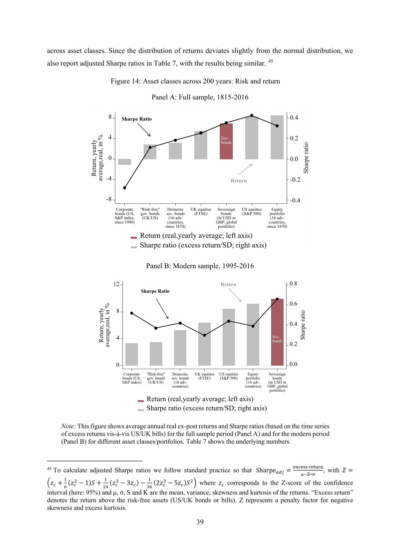
39
across asset classes. Since the distribution of returns deviates slightly from the normal distribution, we
also report adjusted Sharpe ratios in Table 7, with the results being similar. 45
Figure 14: Asset classes across 200 years: Risk and return
Panel A: Full sample, 1815-2016
Panel B: Modern sample, 1995-2016
Note: This figure shows average annual real ex-post returns and Sharpe ratios (based on the time series of excess returns vis-à-vis US/UK bills) for the full sample period (Panel A) and for the modern period (Panel B) for different asset classes/portfolios. Table 7 shows the underlying numbers.
45 To calculate adjusted Sharpe ratios we follow standard practice so that Sharpe𝑠𝑠𝐵𝐵𝑗𝑗 = excess return
µ−Z∗σ, with 𝑍𝑍 =
�𝑧𝑧𝑐𝑐 + 16
(𝑧𝑧𝑐𝑐2 − 1)𝑆𝑆 + 124
(𝑧𝑧𝑐𝑐3 − 3𝑧𝑧𝑐𝑐) − 136
(2𝑧𝑧𝑐𝑐3 − 5𝑧𝑧𝑐𝑐)𝑆𝑆2� where 𝑧𝑧𝑐𝑐 corresponds to the Z-score of the confidence interval (here: 95%) and μ, σ, S and K are the mean, variance, skewness and kurtosis of the returns. “Excess return” denotes the return above the risk-free assets (US/UK bonds or bills). Z represents a penalty factor for negative skewness and excess kurtosis.
Sov.bonds
Sharpe Ratio
Return
-0.4
-0.2
0.0
0.2
0.4
Shar
pe ra
tio
-8
-4
0
4
8
Ret
urn,
yea
rlyav
erag
e,re
al, i
n %
Corporatebonds (US,S&P index,since 1900)
Domesticsov. bonds
(16 adv.countries,
since 1870)
UK equities(FTSE)
Sovereignbonds
(in USD orGBP, global
portfolio)
Equityportfolio(16 adv.
countries,since 1870)
US equities(S&P 500)
"Risk-free"gov. bonds(UK/US)
Return (real,yearly average; left axis)Sharpe ratio (excess return/SD; right axis)
Sov.bonds
Sharpe RatioReturn
0.0
0.2
0.4
0.6
0.8
Shar
pe ra
tio
0
4
8
12
Ret
urn,
yea
rlyav
erag
e,re
al, i
n %
Corporatebonds (US,S&P index)
Domesticsov. bonds
(16 adv.countries)
UK equities(FTSE)
Sovereignbonds
(in USD orGBP, global
portfolio)
Equityportfolio(16 adv.
countries)
US equities(S&P 500)
"Risk-free"gov. bonds(UK/US)
Return (real,yearly average; left axis)Sharpe ratio (excess return/SD; right axis)
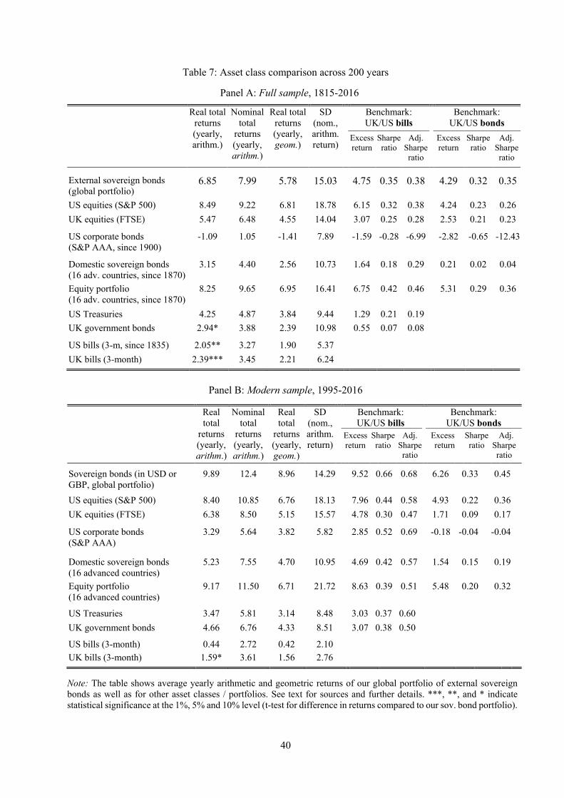
40
Table 7: Asset class comparison across 200 years
Panel A: Full sample, 1815-2016
Real total returns (yearly, arithm.)
Nominal total
returns (yearly, arithm.)
Real total returns (yearly, geom.)
SD (nom., arithm. return)
Benchmark: UK/US bills
Benchmark: UK/US bonds
Excess return
Sharpe ratio
Adj. Sharpe ratio
Excess return
Sharpe ratio
Adj. Sharpe ratio
External sovereign bonds (global portfolio)
6.85 7.99 5.78 15.03 4.75 0.35 0.38 4.29 0.32 0.35
US equities (S&P 500) 8.49 9.22 6.81 18.78 6.15 0.32 0.38 4.24 0.23 0.26 UK equities (FTSE) 5.47 6.48 4.55 14.04 3.07 0.25 0.28 2.53 0.21 0.23 US corporate bonds (S&P AAA, since 1900)
-1.09 1.05 -1.41 7.89 -1.59 -0.28 -6.99 -2.82 -0.65 -12.43
Domestic sovereign bonds (16 adv. countries, since 1870)
3.15 4.40 2.56 10.73 1.64 0.18 0.29 0.21 0.02 0.04
Equity portfolio (16 adv. countries, since 1870)
8.25 9.65 6.95 16.41 6.75 0.42 0.46 5.31 0.29 0.36
US Treasuries 4.25 4.87 3.84 9.44 1.29 0.21 0.19 UK government bonds 2.94* 3.88 2.39 10.98 0.55 0.07 0.08 US bills (3-m, since 1835) 2.05** 3.27 1.90 5.37 UK bills (3-month) 2.39*** 3.45 2.21 6.24
Panel B: Modern sample, 1995-2016
Real total
returns (yearly, arithm.)
Nominal total
returns (yearly, arithm.)
Real total
returns (yearly, geom.)
SD (nom., arithm. return)
Benchmark: UK/US bills
Benchmark: UK/US bonds
Excess return
Sharpe ratio
Adj. Sharpe ratio
Excess return
Sharpe ratio
Adj. Sharpe ratio
Sovereign bonds (in USD or GBP, global portfolio)
9.89 12.4 8.96 14.29 9.52 0.66 0.68 6.26 0.33 0.45
US equities (S&P 500) 8.40 10.85 6.76 18.13 7.96 0.44 0.58 4.93 0.22 0.36 UK equities (FTSE) 6.38 8.50 5.15 15.57 4.78 0.30 0.47 1.71 0.09 0.17 US corporate bonds (S&P AAA)
3.29 5.64 3.82 5.82 2.85 0.52 0.69 -0.18 -0.04 -0.04
Domestic sovereign bonds (16 advanced countries)
5.23 7.55 4.70 10.95 4.69 0.42 0.57 1.54 0.15 0.19
Equity portfolio (16 advanced countries)
9.17 11.50 6.71 21.72 8.63 0.39 0.51 5.48 0.20 0.32
US Treasuries 3.47 5.81 3.14 8.48 3.03 0.37 0.60 UK government bonds 4.66 6.76 4.33 8.51 3.07 0.38 0.50 US bills (3-month) 0.44 2.72 0.42 2.10 UK bills (3-month) 1.59* 3.61 1.56 2.76
Note: The table shows average yearly arithmetic and geometric returns of our global portfolio of external sovereign bonds as well as for other asset classes / portfolios. See text for sources and further details. ***, **, and * indicate statistical significance at the 1%, 5% and 10% level (t-test for difference in returns compared to our sov. bond portfolio).

41
Across the two centuries under study, a global portfolio of external sovereign bonds shows favorable risk-
return properties compared with other financial assets, with substantial variation in relative performance
across time. On average, only US equities and the portfolio of advanced country equities show a higher
return. In the full sample, the return on external sovereign bonds is significantly higher than that of US
corporate bonds, UK equities, US or UK government bonds and that of the portfolio of domestic sovereign
bonds from 16 countries. Our external bond portfolio also shows a high Sharpe ratio, on the same level
as US equities, and exceeding that of the other asset classes. The CAPM analysis in Appendix B7 further
suggests that the beta for this asset class is low, especially in the historical sample (well below 0.5),
suggesting that external bonds provided a diversification service with respect to US/UK equities.
In the modern period (post-1994), foreign-currency sovereign bonds fare even better (Panel B in Figure
14 and Table 7). The Sharpe ratio is highest among the asset classes under study and the returns exceed
those on US and UK equities, on US corporate bonds, and on advanced country equity and domestic bond
portfolios. High average coupon rates during the modern period coupled with the paucity of serious credit
events have delivered a high ex-post return for this asset class in the past three decades. However, this
does not imply that this benign combination is set to become the “new normal” for the sovereign bond
market, as rising debt difficulties in developing countries can morph into defaults abruptly (Reinhart,
Reinhart, and Trebesch 2018).
6.3. Total returns during major financial crises
We next examine the performance of each asset class around selected major crises in financial center(s)
that have different features, as to their global effects. In particular, we compare the cumulative total return
of US stocks, US Treasuries, and external sovereign bonds (our sample of serial defaulters) three years
before and after (i) the New York Panic of 1907 (crash month: October), (ii) the Great Depression (crash
month: October 1929), and (iii) the recent Financial Crisis (crash month: Sept. 2008). Figure 15 shows
the resulting monthly return series, indexed to 100 in the starting month of the crisis. The results from
these case studies are broadly in line with the aggregate statistics summarized above. External sovereign
bonds show higher cumulative returns than stocks in two of the three spells (by the end of year three).
The returns on our global portfolio also tend to be less volatile than those of stocks. Compared with US
Treasuries, external sovereign bonds fare better in 1907, but significantly worse during the Great
Depression. In the Financial Crisis of 2008, external sovereign bonds deliver worse returns compared
with US bonds at the height of the crisis, but subsequently show a much better performance.
Summing up, these findings suggest that sovereign bonds of periphery countries can provide investors
with a viable diversification strategy and, absent a surge in the incidence of default, comparatively high
returns. The high average coupon payments on external sovereign bonds help to stabilize total returns
when prices are volatile.
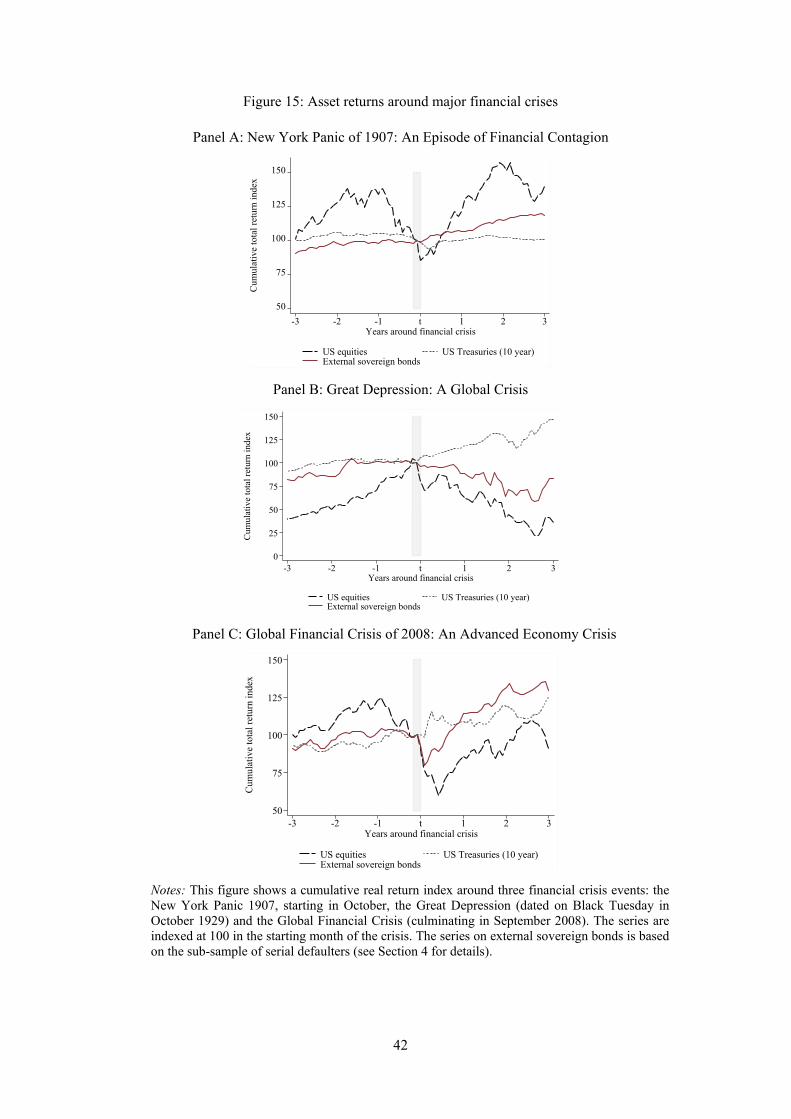
42
Figure 15: Asset returns around major financial crises
Panel A: New York Panic of 1907: An Episode of Financial Contagion
Panel B: Great Depression: A Global Crisis
Panel C: Global Financial Crisis of 2008: An Advanced Economy Crisis
Notes: This figure shows a cumulative real return index around three financial crisis events: the New York Panic 1907, starting in October, the Great Depression (dated on Black Tuesday in October 1929) and the Global Financial Crisis (culminating in September 2008). The series are indexed at 100 in the starting month of the crisis. The series on external sovereign bonds is based on the sub-sample of serial defaulters (see Section 4 for details).
50
75
100
125
150
Cum
ulat
ive
tota
l ret
urn
inde
x
-3 -2 -1 t 1 2 3Years around financial crisis
US equities US Treasuries (10 year)External sovereign bonds
0
25
50
75
100
125
150
Cum
ulat
ive
tota
l ret
urn
inde
x
-3 -2 -1 t 1 2 3Years around financial crisis
US equities US Treasuries (10 year)External sovereign bonds
50
75
100
125
150
Cum
ulat
ive
tota
l ret
urn
inde
x
-3 -2 -1 t 1 2 3Years around financial crisis
US equities US Treasuries (10 year)External sovereign bonds
43
7. Conclusion
We show that the history of external sovereign bonds is a history of frequent investor profits and
occasional losses. Defaults and haircuts have been a recurring feature in this market, but on average
investors were compensated for the risks they took also when compared with other asset classes such as
equity. We have uncovered an excess return over the past two centuries, which we deem as informative
about the attitude of investors toward risk. The observed ex-post spreads are wide, even taking into
account losses associated with default and debt restructuring. Central to this finding are the comparatively
rich coupons offered by this asset class.
The data we have compiled will allow for a reassessment of how markets price sovereign risk and how
investors form beliefs about crash probabilities in emerging markets. A growing literature emphasizes
expectations errors on the part of global investors. During periods of optimism and financial stability,
creditors may become dismissive of the possibility of default and expect full repayment of the rich
coupons offered in this asset class, resulting in lending booms. This recurrent pattern of “market
exuberance” is integral to the narrative in Reinhart and Rogoff (2009) and is explored theoretically in
Gennaioli and Shleifer (2018). Future work could use our data to test these notions, as well as new and
old asset pricing theories, in particular models of long-run risk (Bansal and Yaron 2004) and disaster risk
(Barro 2006; Gabaix 2012).
The paper will also facilitate research on sovereign defaults and their resolution (e.g., Broner et al. 2014;
Corsetti, Erce, and Uy 2018; Erce and Mallucci 2018; Gourinchas, Martin, and Messer 2018; Lorenzoni
and Werning 2018; Aguiar et al. 2019). In particular, we see the need to reexamine our results from the
vantage point of debtor countries and with a view to debt sustainability. What is the appropriate scope of
debt relief when countries fall into debt distress? How can serial restructurings and delays in crisis
resolution be reduced? And, importantly, what motivates countries to pay the large observed premia to
their foreign creditors?

44
References
Aguiar, Mark and Manuel Amador (2014). Sovereign Debt. In: Gopinath, Gita, Elhanan Helpman, and
Kenneth Rogoff (ed.) Handbook of International Economics, Vol. 4, Amsterdam: Elsevier, pp.
647-687.
Aguiar, Mark, Manuel Amador, Hugo Hopenhayn and Iván Werning (2019). Take the Short Route:
Equilibrium Default and Debt Maturity. Econometrica, 87(2), 423-462.
Aguiar, Mark and Gita Gopinath (2006). Defaultable Debt, Interest Rates and the Current Account.
Journal of International Economics, 69(1), 64-83.
Aguiar, Mark, Satyajit Chatterjee, Harold Cole, and Zachary Stangebye (2016). Quantitative Models of
Sovereign Debt Crises. In: Taylor, John B. and Harald Uhlig (ed) Handbook of Macroeconomics,
Vol. 2, Saint Louis: Elsevier, pp. 1697-1755.
Alquist, Ron (2010). How important is liquidity risk for sovereign bond risk premia? Evidence from the
London stock exchange. Journal of International Economics, 82(2), 219-229.
Altman, Edward I. (2011). Default Recovery Rates and Lgd in Credit Risk Modelling and Practice. In:
Lipton, Alexander and Andrew Rennie (ed) The Oxford Handbook of Credit Derivatives , Oxford:
Oxford University Press, pp 39-66.
Amador, Manuel (2012). Sovereign Debt and The Tragedy of the Commons. Mimeo.
Andritzky Jochen R. and Julian Schumacher (2018). Long-Term Returns in Distressed Sovereign Bond
Markets: How Did Investors Fare? Paper presented at the 2018 VfS conference.
Arellano, Cristina (2008). Default Risk and Income Fluctuations in Emerging Economies. American
Economic Review, 98(3), 690-712.
Asonuma, Tamon and Hyungseok Joo (2018). Sovereign Debt Restructurings: Delays in Negotiations
with Risk Averse Creditors. Mimeo.
Asonuma, Tamon and Christoph Trebesch (2016). Sovereign Debt Restructurings: Preemptive or Post-
default. Journal of the European Economic Association, 14(1), 175-214.
Asonuma, Tamon, Dirk Niepelt, and Romain Ranciere (2017). Sovereign Bond Prices, Haircuts and
Maturity. NBER Working Paper 23864.
Asquith, Paul, David W. Mullins, and Eric D. Wolff (1989). Original Issue High Yield Bonds: Aging
Analyses of Defaults, Exchanges, and Calls. Journal of Finance, 44(4), 923-952.
Bansal, Ravi and Amir Yaron (2004). Risks for the Long Run: A Potential Resolution of Asset Pricing
Puzzles. Journal of Finance, 59(4), 1481-1509.
Bank of International Settlements (2018). BIS Quarterly Review, March 2018

45
Barro, Robert J. (2006). Rare Disasters and Asset Markets in the Twentieth Century. Quarterly Journal
of Economics 121(3), 823-866.
Barro, Robert J. and José F. Ursua (2008). Macroeconomic Crises since 1870. Brookings Papers on
Economic Activity, Spring, 255-350.
Borri, Nicola and Adrien Verdelhan (2015). Sovereign Risk Premia. Mimeo.
Broner, Fernando, Aitor Erce, Alberto Martin, and Jaume Ventura, 2014. Sovereign Debt Markets in
Turbulent Times: Creditor Discrimination and Crowding-out Effects, Journal of Monetary
Economics, 61(C), 114-142.
Broner, Fernando, Guido Lorenzoni, and Sergio L. Schmukler (2013). Why Do Emerging Economies
Borrow Short Term? Journal of the European Economic Association, 11(s1),67-100.
Broner, Fernando, Alberto Martin, and Jaume Ventura (2010). Sovereign Risk and Secondary Markets.
American Economic Review, 100(4), 1523-55.
Bulow, Jeremy and Kenneth S. Rogoff (1989). A Constant Recontracting Model of Sovereign Debt.
Journal of Political Economy, 97(1), 155-178.
Campbell, John Y. (2003). Consumption-based Asset Pricing, In: Constantinides, George M., Milton
Harris and René M. Stulz (ed). Handbook of the Economics of Finance, Burlington: Elsevier, pp.
803-887.
Chabot, Benjamin R., and Christoph J. Kurz (2010). That’s Where the Money Was: Foreign Bias and
English Investment Abroad, 1866–1907. Economic Journal, 120(547), 1056-1079.
Chavaz, Matthieu and Flandreau, Marc (2017). “High & Dry”: The Liquidity and Credit of Colonial and
Foreign Government Debt and the London Stock Exchange (1880–1910). The Journal of
Economic History, 77(3), 653-691.
Chen, Long, Pierre Collin-Dufresne, and Robert S. Goldstein (2009). On the Relation Between the Credit
Spread Puzzle and the Equity Premium Puzzle, Review of Financial Studies, 22(9), 3367-3409.
Chen, Hui (2010). Macroeconomic Conditions and the Puzzles of Credit Spreads and Capital Structure.
Journal of Finance, 65(6), 2171-2212.
Corsetti, Giancarlo, Aitor Erce, and Timothy Uy (2018). Debt Sustainability and the Terms of Official
Support. CEPR Discussion Paper 13292.
Cruces, Juan J. and Christoph Trebesch (2013). Sovereign Defaults: The Price of Haircuts. American
Economic Journal: Macroeconomics, 5(3), 85-117.
Dimson, Elroy, Paul R. Marsh, and Mike Staunton (2001). Triumph of the Optimists: 101 Years of Global
Investment Returns. Princeton: Princeton University Press.

46
Drelichman, Mauricio and Hans-Joachim Voth (2011). Serial Defaults, Serial Profits: Returns to
Sovereign Lending in Habsburg Spain, 1566–1600. Explorations in Economic History, 48(1), 1-
19.
Duffie, Darrell (2011). Measuring Corporate Default Risk. Oxford: Oxford University Press
Duffie, Darrell, Lasse Pedersen, and Kenneth Singleton (2003). Modeling Sovereign Yield Spreads: A
Case Study of Russian Debt, Journal of Finance, 58(1), 119-159.
Eaton, Jonathan, and Mark Gersovitz (1981). Debt with Potential Repudiation: Theoretical and Empirical
Analysis. Review of Economic Studies, 48(2), 289-309.
Edelstein, Michael (1982). Overseas Investment in the Age of High Imperialism: The United Kingdom,
1850-1914. New York: Columbia University Press.
Eichengreen, Barry and Richard Portes (1988). Foreign Lending in the Interwar Years: The Bondholders’
Perspective. CEPR Discussion Paper No 273.
Eichengreen, Barry and Richard Portes (1991). After the Deluge: Default, Negotiation, and Readjustment
during the Interwar Years. In: Eichengreen, Barry and Peter H. Lindert, The International Debt
Crisis in Historical Perspective. Cambridge, MA: MIT Press, pp. 12-47.
Erce, Aitor and Enrico Mallucci (2018). Selective Sovereign Defaults. International Finance Discussion
Papers 1239, Board of Governors of the Federal Reserve System.
Ellison, Martin and Andrew Scott (2020). Managing the UK National Debt 1694–2018. American
Economic Journal: Macroeconomics 12 (3): 227-57.
Esteves, Rui (2013). The bondholder, the sovereign, and the banker: sovereign debt and bondholders'
protection before 1914. European Review of Economic History, 17(4), 389–407.
Fang, Chuck, Julian Schumacher, and Christoph Trebesch (2020). Restructuring sovereign bonds:
holdouts, haircuts and the effectiveness of CACs. ECB Working Paper No 2366.
Ferguson, Niall, and Moritz Schularick (2006). The Empire Effect: The Determinants of Country Risk in
the First Age of Globalization, 1880–1913. Journal of Economic History, 66(2), 283-312.
Gabaix, Xavier (2012). Variable Rare Disasters: An Exactly Solved Framework for Ten Puzzles in Macro-
Finance. Quarterly Journal of Economics, 127(2), 645-700.
Gennaioli, Nicola and Andrei Shleifer (2018) A Crisis of Beliefs: Investor Psychology and Financial
Fragility, Princeton: Princeton University Press.
Giesecke, Kay, Francis A. Longstaff, Stephen Schaefer, and Ilya Strebulaev (2011). Corporate Bond
Default Risk: A 150-year Perspective. Journal of Financial Economics, 102(2), 233-250.
Goetzmann, William N. and Andrey D. Ukhov (2006). British Investment Overseas 1870-1913: A
Modern Portfolio Theory Approach. Review of Finance, 10(2), 261-300.

47
Gorton, Gary and Andrew Metrick (2012). Securitized banking and the run on repo. Journal of Financial
Economics, 104(3), 425-451.
Gourinchas, Pierre-Olivier, Philippe Martin, and Todd E. Messer (2018). The Economics of Sovereign
Debt, Bailouts and the Eurozone Crisis. Mimeo.
Grosse Steffen, Christoph and Maximilian Podstawski (2016). Ambiguity and Time-Varying Risk
Aversion in Sovereign Debt Markets. DIW Berlin Discussion Paper No. 1602.
Homer, Sidney and Richard Sylla (2005). A History of Interest Rates. Hoboken: John Wiley & Sons.
Ilzetzki, Ethan, Carmen M. Reinhart, and Kenneth S. Rogoff (2019). Exchange Rate Arrangements in the
21st Century: Which Anchor Will Hold? Quarterly Journal of Economics, 34(2), 599- 646.
International Center for Finance (2018). Historical Financial Research Data: Investor’s Monthly Manual
1869-1929. New Haven: Yale University.
Jankowitsch, Rainer, Florian Nagler, and Marti Subrahmanyam (2014). The Determinants of Recovery
Rates in the US Corporate Bond Market. Journal of Financial Economics, 114(1), 155-177.
Jordà, Òscar, Katharina Knoll, Dmitry Kuvshinov, Moritz Schularick and Alan M. Taylor (2017). The
Rate of Return on Everything, 1870-2015. NBER Working Paper 24112.
Jorgensen, Erika, and Jeffrey Sachs. (1989). Default and Renegotiation of Latin American Foreign Bonds
in the Interwar Period. In Eichengreen, Barry and Peter H. Lindert (ed.) The International Debt
Crisis in Historical Perspective, Cambridge, MA: MIT Press, pp. 48-85.
J.P. Morgan (1999). Introducing the J.P. Morgan Emerging Markets Bond Index Global (EMBI Global).
Kaminsky, Graciela L. and Pablo Vega-García (2016). Systemic and Idiosyncratic Sovereign Debt Crises,
Journal of the European Economic Association, 4(1), 80-114.
Klingen, Christoph, Beatrice Weder di Mauro, and Jeromin Zettelmeyer. (2004). How Private Creditors
Fared in Emerging Debt Markets, 1970-2000. CEPR Discussion Paper No 4374.
Kocherlakota, Narayana (1996). The Equity Premium: It's Still a Puzzle. Journal of Economic Literature,
34(1), 42-71.
Lindert, Peter H. and Peter J. Morton. (1989). How Sovereign Debt Has Worked. In: Sachs, Jeffrey (ed.)
Developing Country Debt and Economic Performance, Volume 1: The International Financial
System, University of Chicago Press, Chicago & London, pp. 39–106.
Lizarazo, Sandra (2013). Default Risk and Risk Averse International Investors. Journal of International
Economics, 89(2), 317-330
Lorenzoni, Guido and Iván Werning (2018). Slow Moving Debt Crises. Mimeo.
Maggiori, Matteo, Brent Neiman, and Jesse Schreger (2020). International Currencies and Capital
Allocation. Journal of Political Economy, 128(6), 2019-2066.

48
Mauro, Paolo, Nathan Sussman, and Yishay Yafeh (2002). Emerging Market Spreads: Then Versus Now.
Quarterly Journal of Economics, 117(2), 695-733.
Mehra, Rajnish and Edward C. Prescott (1985). The Equity Premium: A Puzzle. Journal of Monetary
Economics, 15(2), 145-161.
Mendoza Enrique and Vivian Yue (2012). A General Equilibrium Model of Sovereign Default and
Business Cycles, Quarterly Journal of Economics, 127(2), 889-946.
Meyer, Josefin (2021). Domestic vs. Foreign Debt: Discrimination in Sovereign Debt Restructurings.
Mimeo.
Michie, Ranald (1987). The New York and London Stock Exchanges, 1850–1914. London: Allen and
Unwin.
Michie, Ranald (2001). The London Stock Exchange: A History. New York: Oxford University Press.
Mitchener, Kris J. and Christoph Trebesch (2021). Sovereign Debt in the 21st Century. NBER Working
Paper 28598, forthcoming, Journal of Economic Literature.
Mitchener, Kris J., and Marc D. Weidenmier, (2010). Supersanctions and Sovereign Debt Repayment.
Journal of International Money and Finance, 29(1), 19-36.
Moody’s (2007). Ultimate Recovery Database.
Moody’s (2011a). Corporate Default and Recovery Rates, 1920-2010. Special Comment.
Moody’s (2011b). Sovereign Default and Recovery Rates, 1983-2010. Special Comment.
Moody’s (2012). Investor Losses in Modern-Era Sovereign Bond Restructurings. Special Comment.
Obstfeld, Maurice, and Alan M. Taylor (2005). Global Capital Markets: Integration, Crisis and Growth.
New York: Cambridge University Press.
Panizza, Ugo, Federico Sturzenegger, and Jeromin Zettelmeyer, (2009). The Economics and Law of
Sovereign Debt and Default. Journal of Economic Literature, 47(3), 651-98.
Pouzo, Demian and Ignacio Presno (2016). Sovereign Default Risk and Uncertainty Premia. American
Economic Journal: Macroeconomics, 8(3), 230-66.
Reinhart, Carmen M. and Kenneth S. Rogoff (2009). This Time is Different: Eight Centuries of Financial
Folly. New Jersey: Princeton University Press.
Reinhart, Carmen M., Kenneth S. Rogoff ,and Miguel A. Savastano. (2003). Debt Intolerance, Brookings
Papers on Economic Activity, 34(1), 1-74.
Reinhart, Carmen M., Vincent Reinhart, and Christoph Trebesch (2018). Capital Flow Cycles: A Long,
Global View. Mimeo.

49
Reinhart, Carmen M. and Christoph Trebesch (2016). Sovereign Debt Relief and its Aftermath. Journal
of the European Economic Association, 14(1), 215-251.
Schlegl, Matthias, Christoph Trebesch and Mark L.J. Wright (2019). The Seniority Structure of Sovereign
Debt. NBER Working Paper 25793.
Standard & Poor’s (2006). Default Study: Sovereign Defaults At 26-Year Low, To Show Little Change
In 2007. In: Standard and Poor’s RatingsDirect, September 28.
Sturzenegger, Federico and Jeromin Zettelmeyer (2006). Debt Defaults and Lessons from a Decade of
Crises. Cambridge: The MIT Press.
Sturzenegger, Federico and Jeromin Zettelmeyer (2008). Haircuts: Estimating Investor Losses in
Sovereign Debt Restructurings, 1998-2005. Journal of International Money and Finance, 27(5),
780–805.
Suter, Christian (1992). Debt Cycles in the World-Economy: Foreign Loans, Financial Crises, and Debt
Settlements, 1820-1990. Boulder: Westview Press.
Winkler, Max (1933). Foreign Bonds: An Autopsy; a Study of Defaults and Repudiations of Government
Obligations, (New York: Roland Swain Company).
Wynne, William H. (1951). State Insolvency and Foreign Bondholders. New Haven: Yale University
Press.
Zettelmeyer, Jeromin, Christoph Trebesch and Mitu Gulati (2013). The Greek Debt Restructuring: An
Autopsy. Economic Policy, 28(75), 513-563.

APPENDIX
A1
Online Appendix to “Sovereign Bonds since Waterloo” Meyer, Reinhart, Trebesch (QJE)
Overview:
Appendix A: Financial and macroeconomic data
Appendix B: Bond prices and investor returns (starting on page A4)
Appendix C: Debt restructurings and haircuts (starting on page A42)
Appendix A: Financial and macroeconomic data
This Appendix lists the data sources on financial and macroeconomic variables used in the paper.
Three-month UK bills, monthly, since 1815 The 3-month UK bill return index in the 19th century builds on data by GFD and includes observations from commercial bills (open market rates of discount). For the years 1815-1823 the data comes from Homer (1967). For 1824-1857, the series is retrieved from the NBER Macrohistory database that draws on the open market rates reported in the UK “Parliamentary papers”. For 1857-1899 the bills data comes from The Economist and the Investor’s Monthly Manual. For 1900-1913, the series comes from the NBER Microhistory database and for 1914-1923 from Morgan (1952). The data since 1924 is retrieved from the Central Statistical Office of the British government.
Three-month US bills, monthly, since 1835 The 3-month US bills return series draws on various sources. From 1835-1918, we use the approximated series by GFD, which is based on the minimum rate of the coupon on US Government bonds and commercial bills. For the years 1835-1862, that data was retrieved from Homer (1967), Martin (1886), The Economist (1854-1861) and the periodical Hunt’s Merchants Magazine (1843-1853). From 1862-1918, data comes from The Financial Review. From 1919 onwards, data is retrieved from the Federal Reserve Bank using 90-day Treasury bills. From 1920 until 1942, the data comes from the Federal Reserve Bank, National Monetary Statistics. From 1942 onwards, we retrieve 3-month US bills returns from the Center for Research in Security Prices (CRSP). CSRP calculates total returns based on a comprehensive database of historical US bills. In each month, a representative Treasury bill is selected that is closest to the target maturity.
US Treasury bonds, monthly, since 1815 The long-term US Treasury bond return index is from GFD and constructed using data by Homer (1967) and Martin (1886) for the years 1815-1862, from The Economist (1854-1861) and from the periodical Hunt’s Merchants Magazine (1843-1853). For 1862-1919 data comes from The Financial Review. From 1920 onwards, the data comes from the Federal Reserve Bank and Salomon Brothers (1995). Whenever possible, we use an index of 10-year bonds. During the 19th century, the available indices also contain

APPENDIX
A2
bonds with a much longer maturity, since average maturities were much longer then. From 1942 on, we rely on the 10-year government total bond return series provided by the CRSP database, which builds on a comprehensive collection of US Treasury bond prices.
UK government bonds, monthly, since 1815 The return index on long-term UK government bonds is from GFD and was compiled from Neal (1990) for 1815-1823, from The Times (1824-1844), from the periodical The Banker’s Magazine (1844-1852), and from the Central Statistical Office of the British government (1853 onwards). Whenever possible, we use an index of 10-year bonds, but in the 19th century, the available indices also contain bonds with a much longer maturity, since average maturities were much longer compared to today.
S&P US Stocks Total Return Index, monthly, since 1815 From 1815 to June 1962, we use the US stock market returns index provided by Schwert (1990). From July 1962 onwards, we use the S&P US Stocks Total Return Index from Standard & Poor’s retrieved from GFD.
FTSE UK Stocks Total Return Index, monthly, since 1815 This index is from GFD and compiled from the following sources: Rostow and Schwartz (1953) which contains data on Bank of England Shares and the East Indies Company from 1815 to 1850, Hayek (1935) from 1851-1867, and Smith and Horne (1934) from 1874 to 1922. Additional sources are the periodical Banker’s Magazine (1907-1933), The Economist (1933-1962), and The Financial Times from 1950 onwards. For more recent decades, the data comes from the Central Statistical Office of the British government for the years 1939-1988 and from Eurostat from 1989 until today.
UK inflation/CPI series, monthly The monthly UK CPI series comes from the Bank of England’s (BoE) historical dataset sheet called “A Millennium of UK Data”, Version 3.1, by Thomas and Dimsdale (2017). From 1914 onwards, we use the spliced monthly consumer price index. For the period before WW1, we use the spliced monthly wholesale/producer price index. These series are those recommended by the BoE.
US CPI series, monthly The monthly “Historical Consumer Price Index for All Urban Consumers” is from the US Bureau of Labor Statistics and starts in 1913. For the period before that we rely on series gathered and cited by Reinhart and Rogoff (2009), in particular from the Historical Statistics of the United States. Note that we only have ten USD bonds in our sample that were issued before 1913.
US Corporate bond total return index, monthly, since 1900 The US corporate bond return series is spliced by combining the returns on the S&P 500 AAA Investment Grade Corporate Bond Index from GFD until 1984 with data from the Bank of America Merrill Lynch US Corp AAA Total Return Index thereafter, which we retrieved from the Federal Reserve Bank of St. Louis database.
References Appendix A (those not cited in the main paper):
British Central Statistical Office (various issues) Annual Abstract of Statistics. London: CSO.
Hayek, Friedrich A. (1935) Prices and Production. London: Routledge.
APPENDIX
A3
Homer, Sidney (1967) A History of Interest Rates. Sydney: Princeton University Press.
Martin, Joseph G. (1886) Martin’s Boston Stock Market: Eighty-eight Years from January 1, 1798 to January 1886. Boston.
Morgan, Edward V. (1952). Studies in British Financial Policy, 1914-1925. London: Macmillan.
Neal, Larry (1990) The Rise of Financial Capitalism: International Capital Markets in the Age of Reason. Cambridge: Cambridge University Press.
NBER Macrohistory database.
Rostow, Walt W. and Anna J. Schwartz (1953) The Growth and Fluctuation of the British Economy 1790-1850, Oxford: Oxford U.P.
Salomon Brothers (1995). Analytical Record of Yields and Yield Spreads. New York: Salomon Brothers.
Schwert, William (1990) Indexes of United States Stock Prices from 1802 to 1987, Journal of Business, 63(3), 399-426
Smith, K.C. and G.F Horne (1934) An index number of securities: 1867-1914, London: Royal Economic Society.
Thomas, Ryland and Nicholas Dimsdale (2017) A Millennium of UK Data, Bank of England OBRA dataset
Newspapers: The Economist, Financial Times, Hunt’s Merchants Magazine.
Periodicals: Investors Monthly Manual, Banker’s Magazine, The Financial Review.
Datasets: Eurostat, US Bureau of Labor Statistics, Federal Reserve Bank National Monetary Statistics, Standard and Poors.

APPENDIX
A4
Appendix B: Bond prices and investor returns
B1. Database of bond prices and returns
This section summarizes the sources and coding for our database of sovereign bond prices and returns across 200 years. As explained in the main text we focus on bonds issued (i) by central governments, (ii) in foreign currency (only US dollar and British pound bonds), (iii) traded and priced on the London or New York Stock Exchanges and (iv) with a fixed coupon rate (no floating rate instruments).
We first discuss the historical data, then move to the modern sample that uses JP Morgan’s EMBI data and then describe the final, merged, 200-year dataset.
Historical bond prices and returns, 1818-1980
For the 19th century we use price data of those external sovereign bonds traded on the London Stock Exchange (LSE). From the early 20th century on, these data are complemented with bonds traded on the New York Stock Exchange (NYSE). New York becomes the dominant market for trading and issuing external sovereign bonds from the mid-1920s onwards.
To identify bonds and their prices we rely on several main sources. The London price data for the early 19th century and until 1870 comes from the Money Market Review, The Economist, Circular to Bankers, Course of the Exchange, and The Banker’s Magazine. For the 1869-1929 period we mostly use LSE pricing data from the Investors Monthly Manual, as provided by Goetzmann and Rouwenhorst at the International Center for Finance at Yale. We extend their data series of LSE sovereign bond prices by 50 years, using quotations from The Economist and Financial Times from 1930 to 1980. For illustration, Figure B1 shows an example of how this source looks like. The bond price data from the NYSE was coded from the “Bank and Quotation Section” of the Commercial Financial Chronicle (from 1905 to 1927 and 1954 to 1978) and from the Bank and Quotation Record (from 1927 to 1954).
Our baseline is to use price data of the last trading or business day of the month. We deviate from this rule only for a few dozen bonds before 1850, when markets were not as developed and liquid. For that period, we use the last available price of a month and, rare occasions, also the average between low and high prices of a month.
Beyond prices, we draw on additional sources to collect the financial and legal characteristics of each bond, in particular amount issued, issue date, maturity, coupon rates, coupon frequency, repayment schedule, guarantees or type of issuer. These are taken from bond manuals such as Fenn’s Compendium of the English and Foreign Funds (1837-1838, 1855, 1857, 1863, 1867, 1869, 1874, 1876, 1883, 1889, 1893); Fortune’s Epitome of the Stock and Public Funds (1800, 1810, 1820, 1824, 1826, 1833, 1838-1839, 1850-1851, 1856); Kimber's Records on Government Debts and other Foreign Securities (1918, 1919, 1922, 1934), Moody's Manuals on Foreign and American Government Securities (yearly 1920-196ex0), and the London Stock Exchange Yearbooks (1877-1878, 1880-1881, 1883-1888, 1890, 1894-

APPENDIX
A5
1895, 1897, 1899-1901, 1905, 1907-1916, 1919-1920, 1925). For the years 1869 to 1929 bond features are also partly provided by the Investors Monthly Manual.
Figure B1: The Economist - example of historical bond price quotes
Figure B2: Bank and Quotation Record - example of historical bond price quotes

APPENDIX
A6
Sample: Our original historical database contains 329,637 monthly bond price quotes of 1,712 bonds traded in London and New York and listed in the original sources under categories such as “Foreign Government”. Upon closer inspection, we drop roughly one third of these observations, so as to get to a homogenous sample of foreign-currency sovereign bonds issued by independent states in US dollars or British pounds.
Specifically, we drop:
• 388 bonds that were issued by a state under colonial status. These are colonial bonds by Antigua and Barbuda, Barbados, Fiji, Ghana, Grenada, Guyana, Hawaii, Hong Kong, Iceland, India, Indonesia, Iran, Jamaica, Kenya, Liberia, Mauritius, Morocco, Newfoundland, Nigeria, Palestine, Philippines, Saint Luca, Sierra Leone, Singapore, Southern Rhodesia, Sri Lanka, Straits Settlement, Sudan, Tanganyika, Trinidad and Tobago, and Zanzibar. This reduces our dataset to 292,000 monthly bond prices.
• 256 sub-national bonds, issued by provinces and municipalities but not the central government, reducing the sample to 233,968 monthly bond prices.
• 80 local currency bonds as well as 7 bonds denominated in other foreign currencies (e.g., German Mark or French Franc).
• 12 bonds that were explicitly guaranteed by other governments, via a respective clause in the bond contract. These include the Greek 1833 bonds whose interest and principal payments were fully guaranteed by Great Britain, France and Russia, or the Austrian 6% guaranteed bond of 1923 which had been issued under the auspices of the League of Nations with guarantees by several European governments. Investor reports of the time regard these bonds not as debt owed by the issuing sovereign but as a liability of the guarantor sovereign. For example, the IMM lists guaranteed bonds in the section of the guaranteeing nation, for example, Great Britain.
• Finally, we exclude three sets of bonds: 10 bonds with erratic and infrequent price quotes (this includes a bond issued by the Confederate States of America in London) 1; 11 exotic bonds such as land warrant bonds or bonds issued by the Khedive of Egypt, but not by Egypt itself; and 37 bonds for which we did not find basic details on coupon, amount issued, or currency.
Our cleaned, final historical dataset after these adjustments covers 209,890 monthly prices of 911 sovereign external bonds issued in US dollar and British pound.
Modern bond period, 1990-2016
For the modern period, we use pricing data provided by JP Morgan, which is available from 1989 onwards, albeit initially for less than five countries that issued bonds in their Brady debt restructurings. More details are provided in the draft. In total the EMBI data cover 56,244 monthly price quotations of 6411 sovereign external bonds issued in US dollar (none is issued in British pound).
1 The so-called Confederate cotton bond was a 20-year security with a 7% coupon payable in British sterling and issued in London. The bonds were illiquid and appear only in our pricing database for a few months.

APPENDIX
A7
Final bond pricing sample, 1815-2016
The merged (historical + modern) bond pricing sample includes a total of 1,552 (911 + 641) foreign-currency sovereign bonds issued and traded in London and New York with 266,146 (209,890 + 56,244) monthly pricing observations of 91 debtor countries. Figure B3 shows the data availability by country.
The apparent gaps in the sovereign bond price and return data series can mainly be explained by the fact that countries tapped New York and London markets irregularly. For example, there are nearly a dozen countries that placed foreign-currency bonds abroad during the interwar years but stopped doing so after WW2. This is particularly true for many advanced countries, for example, in Europe, which now borrow almost exclusively in their own currency (Euro, Swiss Franc, Swedish Krona etc.). The series thus end because old bonds mature and no new bonds enter the dataset. Moreover, the gaps in the 1960s, 1970s and 1980s can be explained by the shift from bond to bank loan financing. In this period sovereign lending was dominated by syndicated bank loans and almost no country issued bonds abroad.
To deal with country break-ups and country mergers we follow conventional practice (in particular the practice in investor manuals and financial reports) and assign the bonds of a country that was broken up or newly united to the respective successor state(s):
Country mergers:
• Australia: Bonds issued by New South Wales and Western Australia are assigned to Australia after unification in 1901.
• Germany: Bonds issued by Prussia are assigned to the German Empire/Germany after 1871. • Italy: Bonds issued by the Kingdom of Sardinia and the Kingdom of the Two Sicilies are
assigned to Italy after the Proclamation of the Kingdom of Italy in 1861. • South Africa: Bonds by the Union of South Africa are assigned to South Africa after 1926. • Yugoslavia: Bonds issued by Serbia and by Montenegro are assigned to Yugoslavia after 1918. • Zimbabwe: Bonds of Southern Rhodesia and Rhodesia are assigned to Zimbabwe after 1965.
Country break-ups:
• Austria-Hungary: Bonds that were issued by the Austrian Empire or the Kingdom of Hungary during the dual monarchy of Austria-Hungary are assigned to Austria or Hungary, respectively.
• Gran Colombia: Bonds issued by Gran Colombia, but assigned to Colombia after the break-up, were linked to Colombia. We use the same procedure for Venezuela. The bonds assigned to Ecuador were not trading in London.
• Ottoman Empire: Bonds of the former Ottoman Empire were assigned to Turkey.
For presentation purposes, in the case of country mergers, we use the name of the new unified country to present the spliced series in Figure B3 and elsewhere (e.g., we denote the series as “Germany” instead of “Germany-Prussia”). Similarly, in the case of country breakups, we use the name of the new country to denote the long-run spliced series (e.g., “Austria” instead of “Austria-Hungary”). Countries that existed only briefly or with limited foreign recognition are not included (e.g., the Confederate States of America).

APPENDIX
A8
Figure B3: Data coverage by country (prices and bid-ask spreads), 1815-2016
AlgeriaAngola
ArgentinaArmeniaAustralia
AustriaAzerbaijan
BelarusBelgium
BelizeBolivia
BrazilBulgaria
CameroonCanada
ChileChina
ColombiaCosta Rica
Cote d'IvoireCroatia
CubaCzechoslovakia
DenmarkDominican Republic
EcuadorEgypt
El SalvadorEstonia
EthiopiaFinlandFranceGabon
GeorgiaGermany
GhanaGreece
GuatemalaHaiti
HondurasHungary
IndonesiaIraq
IrelandItaly
1815 1835 1855 1875 1895 1915 1935 1955 1975 1995 2015
Prices, returns, and bid-ask spreads Prices and returnsYear of independence

APPENDIX
A9
Figure B3 (continued): Data coverage by country (prices and bid-ask spreads), 1815-2016
Note: For brevity, in case of country mergers or country break-ups, we use the name of the new country and omit the historical name (e.g., “Germany” instead of “Germany-Prussia”, “Yugoslavia” instead of “Serbia”, “Turkey” instead of “Ottoman Empire”). Year of Independence from Reinhart and Rogoff (2009). If independence was earlier than 1815 then that year is marked as the year of independence for presentation purposes.
JamaicaJapan
JordanKazakhstan
KenyaLatvia
LebanonLithuaniaMalaysia
MexicoMongoliaMoroccoNamibia
NetherlandsNew Zealand
NicaraguaNigeriaNorwayPakistanPanama
ParaguayPeru
PhilippinesPoland
PortugalRomania
RussiaSenegal
Slovak RepublicSouth AfricaSouth Korea
SpainSri Lanka
SwedenSwitzerland
TanzaniaThailand
Trinidad and TobagoTurkey
UkraineUruguay
VenezuelaVietnam
YugoslaviaZambia
Zimbabwe
1815 1835 1855 1875 1895 1915 1935 1955 1975 1995 2015
Prices, returns, and bid-ask spreads Prices and returnsYear of independence

APPENDIX
A10
B2. Computing Returns: Data and Assumptions Treatment of partial and missed coupon payments: A main challenge to compute total returns on historical sovereign bonds was to collect bond-level data on partial or missed coupon payments during spells of default. We retrieved information on interest servicing during crises from the historical reports of the UK-based Corporation of Foreign Bondholders (CFB) (1876-1944, 1945-1986), the US-based Foreign Bondholders Protective Council (FBPC) (1934-1940, 1945-1950, 1953-1964/67), the Association Belge pour la Défense des Détenteurs de Fonds Publics (1898-1915), and the French Association Nationale des Porteurs Franҫais de Valeurs Mobiliéres (1936-1945, 1948-1974, 1987-1988, 1996). To fill gaps, we also rely on the rich body of investor reports that we gathered for the long-run dataset of prices and restructurings (see Appendix B1 above and Appendix C1 below). Particularly helpful were reprints of (temporary) debt agreements, official announcements, or press releases of the debtor government. We typically extracted the relevant information on interest servicing from text statements such as: “Coupon due May 01, 1932 paid in Jan. 1933 at rate of 60% of the face value of the coupon.” For most bonds we have exact amounts and dates of payments. In case the date of partial coupon payments is missing we assume that the debtor paid on the due date of the coupon (original deadline). In the case we do not find any indication that coupons are missing, we assume that they are fully paid. After gathering all coupon details, we again calculate accrued interest by equally distributing the (full or partial) payments over the original coupon payment period (eq. 5). For example, in the case of a yearly coupon frequency, we calculate returns by dividing the coupon paid by 12 (equal amounts per month).
Accounting for debt restructurings/ haircuts: We account for creditor losses due to a debt restructuring or debt write-off. We do so by combining the old defaulted bonds and the new instruments that creditors receive in the exchange with the implicit assumption that creditors keep the newly restructured bond in the portfolio. We also account for the share of debt written off as well as for potential cash or so-called “goodwill” payments that are made in the wake of a restructuring. More precisely, we create spliced series on prices, coupons and returns by combining the old and new bond in the month of the debt exchange.
In the case of a nominal debt reduction (face value haircut), bondholders receive a reduced total face value in new bonds compared to what they held in their old, defaulted bonds. We account for this by creating a spliced series of old and new bonds for which we multiply all post-restructuring bond prices and coupon payments by the size of the write-off. For example, in the case of a face value reduction of 40%, all future price observations of the new bond series are multiplied by 0.6 (1 minus the write-off of 0.4). Accordingly, to create the spliced series, we would also adjust all future coupon payments on the new bonds by multiplying them by 0.6. Cash payments agreed on in the wake of a debt restructuring, e.g., for the settlement of arrears or as deal “sweeteners”, are accounted for in the month in which they are made. For illustration, we can rewrite our baseline bond return Equation 2 for the month of the restructuring (when old bonds are exchanged into new bonds) as follows:
𝑅𝑅𝑛𝑛𝑠𝑠𝑛𝑛 𝑏𝑏𝑝𝑝𝑛𝑛𝐵𝐵,𝑚𝑚=𝑁𝑁𝑛𝑛𝑠𝑠𝑛𝑛 𝑏𝑏𝑝𝑝𝑛𝑛𝐵𝐵,𝑚𝑚 ∗ (1 − 𝑤𝑤𝑟𝑟𝑖𝑖𝑡𝑡𝑠𝑠𝑤𝑤𝑤𝑤𝑤𝑤) + 𝐶𝐶𝑛𝑛𝑠𝑠𝑛𝑛 𝑏𝑏𝑝𝑝𝑛𝑛𝐵𝐵,𝑚𝑚 ∗ (1 − 𝑤𝑤𝑟𝑟𝑖𝑖𝑡𝑡𝑠𝑠𝑤𝑤𝑤𝑤𝑤𝑤) + 𝐶𝐶𝑠𝑠𝑠𝑠ℎ𝑚𝑚
𝑁𝑁𝑝𝑝𝑝𝑝𝐵𝐵 𝑏𝑏𝑝𝑝𝑛𝑛𝐵𝐵,𝑚𝑚−1− 1

APPENDIX
A11
where 𝑅𝑅𝑛𝑛𝑠𝑠𝑛𝑛 𝑏𝑏𝑝𝑝𝑛𝑛𝐵𝐵,𝑚𝑚 is the spliced return series, 𝑁𝑁𝑝𝑝𝑝𝑝𝐵𝐵 𝑏𝑏𝑝𝑝𝑛𝑛𝐵𝐵,𝑚𝑚−1 is the secondary market price of the old bond in the month prior to the restructuring (or the last pricing observation we have before that), 𝑁𝑁𝑛𝑛𝑠𝑠𝑛𝑛 𝑏𝑏𝑝𝑝𝑛𝑛𝐵𝐵,𝑚𝑚 is the price of the newly issued bond once it starts trading (first month for which we have a pricing observation post-restructuring), 𝑤𝑤𝑟𝑟𝑖𝑖𝑡𝑡𝑠𝑠𝑤𝑤𝑤𝑤𝑤𝑤 is the size of the nominal debt reduction (face value haircut) on the old bonds, 𝐶𝐶𝑛𝑛𝑠𝑠𝑛𝑛 𝑏𝑏𝑝𝑝𝑛𝑛𝐵𝐵,𝑚𝑚 are coupon payments on the new bond, and 𝐶𝐶𝑠𝑠𝑠𝑠ℎ𝑚𝑚 are cash or “goodwill” payments. For the spliced series, the formula is applied accordingly in all months following the restructuring, only that 𝑁𝑁𝑝𝑝𝑝𝑝𝐵𝐵 𝑏𝑏𝑝𝑝𝑛𝑛𝐵𝐵,𝑚𝑚−1 in the denominator is replaced by 𝑁𝑁𝑛𝑛𝑠𝑠𝑛𝑛 𝑏𝑏𝑝𝑝𝑛𝑛𝐵𝐵,𝑚𝑚 ∗(1 − 𝑤𝑤𝑟𝑟𝑖𝑖𝑡𝑡𝑠𝑠𝑤𝑤𝑤𝑤𝑤𝑤), meaning the adjusted price of the new bond lagged by one month. In case the restructuring only involves a rescheduling of maturities but no face value debt reduction, the term 𝑤𝑤𝑟𝑟𝑖𝑖𝑡𝑡𝑠𝑠𝑤𝑤𝑤𝑤𝑤𝑤would be zero, but the change in maturities should be reflected in the secondary market price of the new bond (this type of debt exchange is sometimes called “debt reprofiling”).
For the historical restructuring cases, Box B1 shows how old and new bonds were linked as well as the conversion rate (1 − 𝑤𝑤𝑟𝑟𝑖𝑖𝑡𝑡𝑠𝑠𝑤𝑤𝑤𝑤𝑤𝑤) with which coupons and prices are multiplied for the spliced return series of the new bonds. The table includes those restructured bonds for which prices were available.
Box B1 Linking old and new bonds to create long-run return series, historical restructurings
Country
Bond name
Bond ID
Successor bond name
Successor bond ID
Conversion rate of old into new bonds
Date of bond exchange
First pricing observ. of successor bond
Bolivia 6% Loan of 1872 179 debt buyback 0.476 03/1880 03/1880 Brazil 4% Loan of 1889 186 1.5 (4)% Loan (Plan A); 3.75%
Bonds of 1944 211;258 Plan A: 1;
Plan B: 0.5 11/1943 04/1944
Brazil 4% Loan of 1901-1905
185 1.5 (4)% Loan (Plan A); 3.5% Bonds of 1944 (Plan B)
238;239 Plan A: 1; Plan B: 0.5
11/1943 04/1944
Brazil 5% Bonds of 1898 187 3.375 (5)% Loan (Plan A); 3.75% Bonds of 1944
234;235 Plan A: 1; Plan B: 0.8
11/1943 04/1944
Brazil 5% Loan of 1931 (series A)
245 3.375 (6.5)% Loan (Plan A); 3.75% Bonds of 1944
246;247 Plan A: 1; Plan B: 0.8
11/1943 04/1944
Brazil 5% Loan of 1931(series B)
248 3.375 (6.5)% Loan (Plan A); 3.75% Bonds of 1944
249;250 Plan A: 1; Plan B: 0.8
11/1943 04/1944
Brazil 5% Loan of 1913 203 1.75 (5)% Loan (Plan A); 3.75% Bonds of 1944
240;241 Plan A: 1; Plan B: 0.5
11/1943 04/1944
Brazil 5% Loan of 1914 188 3.375 (5)% Loan (Plan A); 3.75% Bonds of 1944
242;243 Plan A: 1; Plan B: 0.8
11/1943 04/1944
Brazil 6.5% Loan of 1927 208 3.375 (6.5)% Loan (Plan A); 3.75% Bonds of 1944
213;244 Plan A: 1; Plan B: 0.5
11/1943 04/1944
Brazil 6.5% Loan of 1926 224 3.375 (6.5)% Loan (Plan A); 3.75% Bonds of 1944
225;232 Plan A: 1; Plan B: 0.8
11/1943 07/1944
Brazil 6.5% Loan of 1927 226 3.375 (6.5)% Loan (Plan A); 3.75% Bonds of 1944
227;233 Plan A: 1; Plan B: 0.8
11/1943 07/1944
Brazil 7% Loan of 1922 228 3.5 (7)% Loan (Plan A); 3.75% Bonds of 1944
229;231 Plan A: 1; Plan B: 0.8
11/1943 07/1944
Brazil 8% Loan of 1921 222 3.5 (8)% Loan (Plan A); 3.75% Bonds of 1944
223;230 Plan A: 1; Plan B: 0.8
11/1943 07/1944
Brazil 5% Bonds of 1895 192 1.75 (5)% Loan (Plan A); 3.75% Bonds of 1944
212;251 Plan A: 1; Plan B: 0.5
11/1943 09/1945
Brazil 4% Railway Bonds of 1911
199 1.5 (4)% Loan (Plan A); 3.75% Bonds of 1944 (Plan B)
252;253 Plan A: 1; Plan B: 0.5
11/1943 10/1945
Chile 4.5% Bonds of 1887 316 1.5-3% Mixed Bonds of 1948 343 1 03/1948 03/1953 Chile 5% Loan of 1911 (1st
series) 322 1.5-3% Mixed Bonds of 1948 343 1 03/1948 03/1953
Chile 6% Loan of 1926 330 1.5-3% Mixed Bonds of 1948 343 1 03/1948 03/1953 Chile 6% Bonds of 1926 348 1.5-3% of 1948 349 1 03/1948 12/1948 Chile 6% Bonds of 1927 350 1.5-3% of 1948 349 1 03/1948 12/1948

APPENDIX
A12
Chile 6% Bonds of 1928 352 1.5-3% of 1948 349 1 03/1948 12/1948 Chile 6% Bonds of 1929 346 1.5-3% of 1948 349 1 03/1948 12/1948 Chile 6% Bonds of 1930 347 1.5-3% of 1948 349 1 03/1948 12/1948 Chile 6% Railway Bonds of
1928 351 1.5-3% of 1948 349 1 03/1948 12/1948
Chile 7% of 1922, due 1942 345 1.5-3% of 1948 349 1 03/1948 12/1948 Chile 7% of 1922, due 1942
(assented 1935) 356 1.5-3% Mixed Bonds of 1948 343 1 03/1948 12/1948
Chile 6% Bonds of 1926 (assented 1935)
357 1.5-3% Mixed Bonds of 1948 343 1 03/1948 12/1948
Chile 6% Bonds of 1927 (assented 1935)
358 1.5-3% Mixed Bonds of 1948 343 1 03/1948 12/1948
Chile 6% Bonds of 1928 (assented 1935)
355 1.5-3% Mixed Bonds of 1948 343 1 03/1948 12/1948
Chile 6% Bonds of 1929 (assented 1935)
353 1.5-3% Mixed Bonds of 1948 343 1 03/1948 12/1948
Chile 6% Bonds of 1930 (assented 1935)
354 1.5-3% Mixed Bonds of 1948 343 1 03/1948 12/1948
Chile 6% Railway Bonds of 1928 (assented 1935)
359 1.5-3% Mixed Bonds of 1948 343 1 03/1948 12/1948
Colombia 1-6% active bonds of 1845
392 4.5-4.75% Bonds of 1873 244 0.34 12/1873 07/1874
Colombia 2-3% Bonds of 1860 391 4.5-4.75% Bonds of 1873 244 0.66 12/1873 07/1874 Colombia 6% Bonds of 1927 399 3% of 1940 401 1 06/1941 07/1941 Colombia 6% Bonds of 1928 398 3% of 1940 401 1 06/1941 07/1941 Colombia 4.5-4.75% Bonds of
1873 389 1.5-3% Bonds of 1896 388 1 12/1896 10/1897
Colombia 6% Bonds of 1822,1824
397 1-6% Bonds of 1845 392 1 01/1845 12/1845
Costa Rica 7% Loan of 1926 408 Refunding 1.5-3% of 1952 409 1 11/1952 03/1954 Costa Rica 6% Bonds of 1871
(series 1) 405 5% Bonds of 1886 (series
A);4-5% Bonds of 1886 (series B)
402;403 1 06/1885 09/1886
Costa Rica 7% Bonds of 1872 407 4-5% Bonds of 1886 (series B) 403 0.5 06/1885 09/1886 Costa Rica 4-5% Bonds of 1886
(series B) 403 4-5% Bonds of 1911 404 0.65 12/1910 12/1911
Costa Rica 5% Bonds of 1886 (series A)
402 4-5% Bonds of 1911 404 0.75 12/1910 12/1911
Cuba 5.5% Bonds of 1930, due 1940
418 4.5% of 1937 420 1.1 02/1938 07/1938
Czechoslovakia 8% Bonds of 1922/1924
424 debt buyback 0.75 04/1960 12/1960
Ecuador 1-6% Bonds of 1855 454 4.5-5% Bonds of 1891 455 0.4 07/1892 07/1893 Egypt 7% Bonds of 1864 458 7% Bonds of 1877,1880
(dated 1876) 465 1 07/1880 08/1880
Egypt 9% Bonds of 1867 466 7% Bonds of 1877,1880 (dated 1876)
465 1 07/1880 08/1880
Egypt 7% Bonds of 1862 462 7% Bonds of 1877,1880 (dated 1876), 5% preferred Bonds of 1877,1880
465;464 1 11/1876 12/1876
Egypt 7% Bonds of 1862 (series 2)
463 7% Bonds of 1877,1880 (dated 1876), 5% preferred Bonds of 1877,1880
465;464 1 11/1876 12/1876
Egypt 7% Bonds of 1868 459 7% Bonds of 1877,1880 (dated 1876), 5% preferred Bonds of 1877,1880
465;464 1 11/1876 12/1876
Egypt 7% Bonds of 1873 460 7% Bonds of 1877,1880 (dated 1876), 5% preferred Bonds of 1877,1880
465;464 1 11/1876 12/1876
El Salvador 6% Bonds of 1908 468 6% Loan of 1923 (Series B) 470 1 09/1923 02/1924 El Salvador 7% Bonds of 1915 469 6% Loan of 1923 (Series B) 470 1 09/1923 02/1924 Greece 5% Bonds of
1824,1825 506 5% Loan of 1879 516 0.3 12/1878 07/1880
Guatemala 5% Loan of 1856 529 4% Bonds of 1888 530 1 03/1888 09/1888 Guatemala 6% Bonds of 1869 532 4% Bonds of 1888 530 1 03/1888 09/1888 Guatemala 4% Bonds of 1888 530 4% Bonds of 1895 531 0.75 07/1895 12/1895 Italy 7% Loan of 1925 565 1-3% of 1947 566 1 12/1947 12/1947
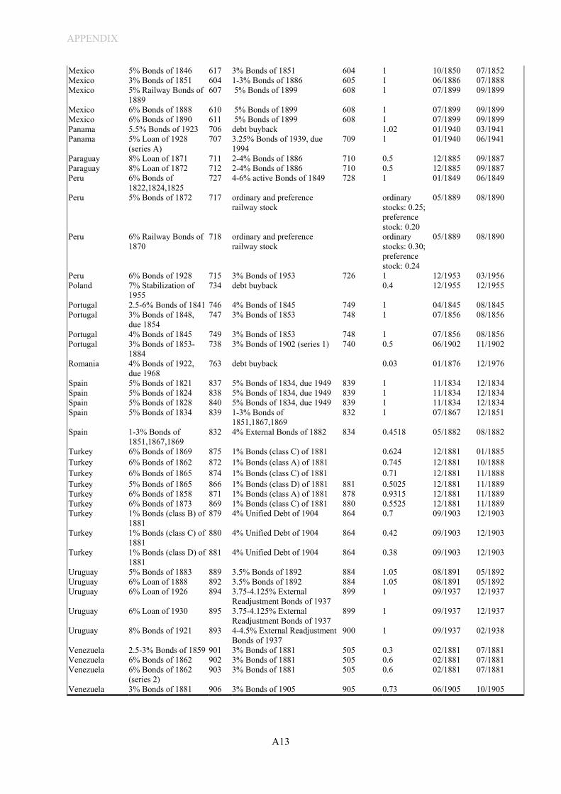
APPENDIX
A13
Mexico 5% Bonds of 1846 617 3% Bonds of 1851 604 1 10/1850 07/1852 Mexico 3% Bonds of 1851 604 1-3% Bonds of 1886 605 1 06/1886 07/1888 Mexico 5% Railway Bonds of
1889 607 5% Bonds of 1899 608 1 07/1899 09/1899
Mexico 6% Bonds of 1888 610 5% Bonds of 1899 608 1 07/1899 09/1899 Mexico 6% Bonds of 1890 611 5% Bonds of 1899 608 1 07/1899 09/1899 Panama 5.5% Bonds of 1923 706 debt buyback 1.02 01/1940 03/1941 Panama 5% Loan of 1928
(series A) 707 3.25% Bonds of 1939, due
1994 709 1 01/1940 06/1941
Paraguay 8% Loan of 1871 711 2-4% Bonds of 1886 710 0.5 12/1885 09/1887 Paraguay 8% Loan of 1872 712 2-4% Bonds of 1886 710 0.5 12/1885 09/1887 Peru 6% Bonds of
1822,1824,1825 727 4-6% active Bonds of 1849 728 1 01/1849 06/1849
Peru 5% Bonds of 1872 717 ordinary and preference railway stock
ordinary stocks: 0.25; preference stock: 0.20
05/1889 08/1890
Peru 6% Railway Bonds of 1870
718 ordinary and preference railway stock
ordinary stocks: 0.30; preference stock: 0.24
05/1889 08/1890
Peru 6% Bonds of 1928 715 3% Bonds of 1953 726 1 12/1953 03/1956 Poland 7% Stabilization of
1955 734 debt buyback 0.4 12/1955 12/1955
Portugal 2.5-6% Bonds of 1841 746 4% Bonds of 1845 749 1 04/1845 08/1845 Portugal 3% Bonds of 1848,
due 1854 747 3% Bonds of 1853 748 1 07/1856 08/1856
Portugal 4% Bonds of 1845 749 3% Bonds of 1853 748 1 07/1856 08/1856 Portugal 3% Bonds of 1853-
1884 738 3% Bonds of 1902 (series 1) 740 0.5 06/1902 11/1902
Romania 4% Bonds of 1922, due 1968
763 debt buyback 0.03 01/1876 12/1976
Spain 5% Bonds of 1821 837 5% Bonds of 1834, due 1949 839 1 11/1834 12/1834 Spain 5% Bonds of 1824 838 5% Bonds of 1834, due 1949 839 1 11/1834 12/1834 Spain 5% Bonds of 1828 840 5% Bonds of 1834, due 1949 839 1 11/1834 12/1834 Spain 5% Bonds of 1834 839 1-3% Bonds of
1851,1867,1869 832 1 07/1867 12/1851
Spain 1-3% Bonds of 1851,1867,1869
832 4% External Bonds of 1882 834 0.4518 05/1882 08/1882
Turkey 6% Bonds of 1869 875 1% Bonds (class C) of 1881 0.624 12/1881 01/1885 Turkey 6% Bonds of 1862 872 1% Bonds (class A) of 1881 0.745 12/1881 10/1888 Turkey 6% Bonds of 1865 874 1% Bonds (class C) of 1881 0.71 12/1881 11/1888 Turkey 5% Bonds of 1865 866 1% Bonds (class D) of 1881 881 0.5025 12/1881 11/1889 Turkey 6% Bonds of 1858 871 1% Bonds (class A) of 1881 878 0.9315 12/1881 11/1889 Turkey 6% Bonds of 1873 869 1% Bonds (class C) of 1881 880 0.5525 12/1881 11/1889 Turkey 1% Bonds (class B) of
1881 879 4% Unified Debt of 1904 864 0.7 09/1903 12/1903
Turkey 1% Bonds (class C) of 1881
880 4% Unified Debt of 1904 864 0.42 09/1903 12/1903
Turkey 1% Bonds (class D) of 1881
881 4% Unified Debt of 1904 864 0.38 09/1903 12/1903
Uruguay 5% Bonds of 1883 889 3.5% Bonds of 1892 884 1.05 08/1891 05/1892 Uruguay 6% Loan of 1888 892 3.5% Bonds of 1892 884 1.05 08/1891 05/1892 Uruguay 6% Loan of 1926 894 3.75-4.125% External
Readjustment Bonds of 1937 899 1 09/1937 12/1937
Uruguay 6% Loan of 1930 895 3.75-4.125% External Readjustment Bonds of 1937
899 1 09/1937 12/1937
Uruguay 8% Bonds of 1921 893 4-4.5% External Readjustment Bonds of 1937
900 1 09/1937 02/1938
Venezuela 2.5-3% Bonds of 1859 901 3% Bonds of 1881 505 0.3 02/1881 07/1881 Venezuela 6% Bonds of 1862 902 3% Bonds of 1881 505 0.6 02/1881 07/1881 Venezuela 6% Bonds of 1862
(series 2) 903 3% Bonds of 1881 505 0.6 02/1881 07/1881
Venezuela 3% Bonds of 1881 906 3% Bonds of 1905 905 0.73 06/1905 10/1905

APPENDIX
A14
Amortization schedules, sinking funds and bond buybacks (historical bonds): Most bonds in history are not due and payable at maturity (so-called bullet bonds), but have stretched out amortization, often in the form of so-called “sinking fund” arrangements. During the 19th and early 20th century there are two main types of sinking funds in our sample of bonds. The first, simpler type is a fixed sinking fund scheme that is comparable to a linear amortization plan - with equal payments stretching from the end of the grace period until maturity. Second, there are cumulative sinking fund schemes. These follow a non-linear, typically increasing annuity amortization plan written in the bond contract. The sinking fund payments were usually forwarded to a payment agent determined in the bond contract. This agent uses the debt service to amortize the bonds either by a redemption at par to bondholders or via repurchases on the secondary market. Redemption at par is attractive to investors because bonds typically trade at prices below par. For this reason, the allocation of repayments from the sinking funds was often assigned via lottery. In the lottery, the fiscal agent randomly selects a subset of bonds for full repayment, chosen among all outstanding bonds. This exercise is repeated until the sinking fund payments due in that period are depleted. In practice, redemption at par was the exception, while buybacks on the secondary market were the rule. More than 80% of sinking fund bonds issued before WW2 contain buyback clauses that authorized the agent to redeem funds via purchases on the secondary market (at prices below par) rather than via nominal repayments (which is costlier for sovereigns). To compute price-based return series we disregard the possibility that some of the redemptions are made at par because the beneficiaries of the redemption lottery are random and market prices should reflect any expected redemption gains. We also prefer to be conservative and not add up potential capital gains due to redemption at par. As a result, the calculated returns on sinking fund bonds in history can be regarded as a lower bound.
Gold clauses (historical bonds): About 50% of bonds in our pre-WW2 bond price sample include gold clauses. These gold clauses are not taken into account when computing returns since they were not legally binding, especially after the abrogation of the gold clause in the US in 1933 and Britain in 1931. As we discuss in Appendix C below, we find that gold clauses played almost no role in the restructuring agreements, meaning that bonds with or without gold clauses receive the same treatment (haircut). We also found no evidence that creditors holding gold-clause bonds in historical restructurings ask for better terms than those holding bonds without gold clauses.
Currency clauses (historical bonds): Our sample consists of bonds issued and denominated in USD and GBP. In the historical sample, some bonds contain currency clauses that gave creditors the right to receive repayments from the bond in another currency. We include such bonds, but only if the bond’s face value was denoted in either USD or GBP and if creditors have the right to ask for repayment in USD or GBP as well, meaning that bond prices will not contain currency risk. For these bonds we thus disregard the fact that repayments could optionally also be received in another currency. However, we do exclude bonds issued in multiple currencies, meaning that the bond contract lists the bond’s face value in more than one currency and the currency of repayment depends on contractual details, such as the choice of the stock exchange for settlement. This type of bonds potentially contains currency risks and could therefore bias our results. Specifically, we find (and exclude) 35 bonds issued in multiple currencies, namely by the governments of Austria, Denmark, France, Hungary, Ireland, Italy, Netherlands, and Switzerland between 1831 and 1929.

APPENDIX
A15
B3. Comparison with previous studies on sovereign debt returns B3.1. Comparison to Lindert and Morton (1850-1980)
To compare our results to those of the long-run study by Lindert and Morton (1989, LM) we draw on the microdata made available by them for 1028 external bonds issued by 9 large sovereign debtors, namely Argentina, Australia, Brazil, Chile, Egypt, Japan, Mexico, Russia, and Turkey (as cleaned by Esteves 2013). Compared to the paper, the country sample is reduced from nice to 10 countries because the online database provides no details on the 488 government bonds to Canada (only aggregated cash flows for local governments are available for Canada). 2
We start with a conceptual discussion of how IRRs relate to more standard price-based return measures. We explain why the best comparison measure to IRRs are annualized holding period returns (HPRs), which calculate geometric returns over the entire life span of the bonds. We then replicate the LM IRR calculations for each bond and explore the IRR results in a more disaggregated way than in the LM paper, in particular by distinguishing between sovereign, sub-sovereign (municipal) and corporate bonds. In the last and main step, we compare the IRRs with total returns measures using our own database. All averages reported here are nominal, which facilitates comparisons.
The replication exercise reveals that the average LM bond returns are driven down for two reasons that are less of a concern in our analysis. First, Russia and Turkey decrease the average return in their small sample. Both countries witnessed major upheaval after WW1 that kept their bonds in default for decades, due to Russia’s Communist revolution and the breakup of the Ottoman Empire, respectively. In our 60-country historical sample, outlier countries and lengthy defaults on a subsample of bonds carry less weight. Second, LM include municipal and corporate bonds, which leads to lower aggregate return, as we show below. We focus on sovereign bonds only, which have higher returns, on average.
The second main take away is that the HPRs from our dataset are very similar to the IRRs of Lindert and Morton (1989), be it in aggregate, on the country level, or at the bond level (we have 219 exact matches). Arithmetic returns, however, are notably higher than both the IRRs and the HPR/geometric returns. This underscored how important it is to not only consider arithmetic returns but also geometric returns, especially for those interested in longer holding periods.
Return concepts: IRRs and price based total return measures
To compare the LM IRR results with total return measures using our dataset we need to compute a price-based return measure that most closely resembles the concept of IRRs. Specifically, we need to trace bond returns from issuance to maturity and then calculate the average annual performance. The best price-based measure to do this is the time-weighted (annualized) holding period return, or annualized HPR, which gives you the yearly rate of return on a bond over a given number of years. When computed from issuance to maturity annualized HPRs are conceptually most similar to IRRs, as both measures show average annual returns over the entire life of the bond.
2 The data is available here: https://economics.ucdavis.edu/people/fzlinder/peter-linderts-webpage/data-and-estimates/sovereign-debt-historical-data-lindert-morton/

APPENDIX
A16
To get to the formula of annualized holding period returns we can start with the standard total return formula for period t (one year) as follows:
𝑅𝑅𝑡𝑡𝑡𝑡𝑝𝑝𝑡𝑡𝑠𝑠𝑝𝑝 =𝑁𝑁𝑡𝑡 + 𝑁𝑁𝑡𝑡−1 + 𝐶𝐶𝑡𝑡
𝑁𝑁𝑡𝑡−1− 1 (B1)
where 𝑁𝑁 stands for the bond price (in the paper we use monthly frequency but aggregated by year, see
Equation 4 above), 𝐶𝐶𝑡𝑡 are coupon payments (also aggregated by year), 𝑃𝑃𝑡𝑡+𝑃𝑃𝑡𝑡−1𝑃𝑃𝑡𝑡−1
is the capital gain and 𝐶𝐶𝑡𝑡𝑃𝑃𝑡𝑡−1
is the coupon yield in year t. Using Equation (B1) we can define our baseline return measure in our
analysis, which is the simple arithmetic average annual return for a specific period (year 1 through T):
𝑅𝑅𝑡𝑡𝑠𝑠𝑟𝑟𝑖𝑖𝑡𝑡ℎ𝑠𝑠𝑚𝑚𝑡𝑡𝑖𝑖𝑐𝑐 =1𝑇𝑇�𝑅𝑅𝑡𝑡𝑡𝑡𝑝𝑝𝑡𝑡𝑠𝑠𝑝𝑝𝑇𝑇
𝑡𝑡=1
(B2)
We can further use Equation (B1) to compute cumulative holding period returns (HPRs) from year t =1 until year T, a measure we also discussed in the paper (Section 4.3):
𝐻𝐻𝑁𝑁𝑅𝑅𝑇𝑇 = (1 + 𝑅𝑅1𝑡𝑡𝑝𝑝𝑡𝑡𝑠𝑠𝑝𝑝) ∗ (1 + 𝑅𝑅2𝑡𝑡𝑝𝑝𝑡𝑡𝑠𝑠𝑝𝑝) ∗ … ∗ (1 + 𝑅𝑅𝑇𝑇𝑡𝑡𝑝𝑝𝑡𝑡𝑠𝑠𝑝𝑝) − 1 (B3) With yearly data, we can annualize these HPRs using the standard formula for geometric returns. Specifically, if we assume that gains are reinvested and losses are accumulated, then we can use Equation (B3) to compute geometric returns for the time span between year t to T, as follows:
𝑅𝑅𝑇𝑇𝑔𝑔𝑠𝑠𝑝𝑝𝑚𝑚𝑠𝑠𝑡𝑡𝑟𝑟𝑖𝑖𝑐𝑐 = 𝑠𝑠𝑎𝑎𝑎𝑎𝑀𝑀𝑠𝑠𝑎𝑎𝑖𝑖𝑧𝑧𝑠𝑠𝑠𝑠 𝐻𝐻𝑁𝑁𝑅𝑅𝑇𝑇 = �(1 + 𝑅𝑅1𝑡𝑡𝑝𝑝𝑡𝑡𝑠𝑠𝑝𝑝) ∗ (1 + 𝑅𝑅2𝑡𝑡𝑝𝑝𝑡𝑡𝑠𝑠𝑝𝑝) ∗ … ∗ (1 + 𝑅𝑅𝑇𝑇𝑡𝑡𝑝𝑝𝑡𝑡𝑠𝑠𝑝𝑝)
𝑇𝑇− 1
𝑅𝑅𝑇𝑇𝑔𝑔𝑠𝑠𝑝𝑝𝑚𝑚𝑠𝑠𝑡𝑡𝑟𝑟𝑖𝑖𝑐𝑐 = �� (1 + 𝑅𝑅𝑡𝑡𝑡𝑡𝑝𝑝𝑡𝑡𝑠𝑠𝑝𝑝)
𝑇𝑇
1�1𝑇𝑇− 1
(B4)
In case the bond price volatility is zero, average arithmetic returns for period t to T equal average geometric returns over the same time span. However, the more volatile 𝑅𝑅𝑡𝑡𝑡𝑡𝑝𝑝𝑡𝑡𝑠𝑠𝑝𝑝 is over time, the larger the difference between arithmetic and geometric returns. For low levels of volatility, geometric returns can well be approximated by subtracting half of the variance from arithmetic returns so that
𝑅𝑅𝑇𝑇𝑔𝑔𝑠𝑠𝑝𝑝𝑚𝑚𝑠𝑠𝑡𝑡𝑟𝑟𝑖𝑖𝑐𝑐 ≈ 𝑅𝑅𝑇𝑇𝑠𝑠𝑟𝑟𝑖𝑖𝑡𝑡ℎ𝑚𝑚𝑠𝑠𝑡𝑡𝑖𝑖𝑐𝑐 −
12𝜎𝜎2
For the comparison with Lindert and Morton (1989) we thus apply the formula for annualized HPRs in Equation (B4) for each bond using bond prices and cash flows from issuance to maturity. We then compare the results from this issuance-to-maturity annualized HPRs with issuance-to-maturity IRRs. The standard formula for IRRs can be written as follows
0 = 𝑁𝑁𝑁𝑁𝑁𝑁 = −𝑁𝑁0 + �𝐶𝐶𝐶𝐶𝑡𝑡
(1 + 𝑅𝑅𝑇𝑇𝐼𝐼𝐼𝐼𝐼𝐼)𝑡𝑡
𝑇𝑇
𝑡𝑡=1
Where 𝑇𝑇 is bond maturity, 𝐶𝐶𝐶𝐶𝑡𝑡 are debt payments (coupon and amortization) in year 𝑡𝑡 and 𝑁𝑁0 is the purchasing price, that is, the issue price of the bond.
(B5)
(B6)

APPENDIX
A17
One can show that 𝑅𝑅𝑇𝑇𝐼𝐼𝐼𝐼𝐼𝐼 from Equation (B6), and the 𝑠𝑠𝑎𝑎𝑎𝑎𝑀𝑀𝑠𝑠𝑎𝑎𝑖𝑖𝑧𝑧𝑠𝑠𝑠𝑠 𝐻𝐻𝑁𝑁𝑅𝑅𝑇𝑇 from Equation (B4), are the same under the following assumptions. First, we need to assume that all returns are reinvested. Second and more importantly, both cash flows and the discount rate need to be uniform over the entire holding period of t to T. This is because IRRs are sensitive to the values of particular cash flows in a specific year, while the timing of the cash flows is irrelevant when computing annualized HPRs. Put differently, 𝑠𝑠𝑎𝑎𝑎𝑎𝑀𝑀𝑠𝑠𝑎𝑎𝑖𝑖𝑧𝑧𝑠𝑠𝑠𝑠 𝐻𝐻𝑁𝑁𝑅𝑅𝑇𝑇 will yield the same return as 𝑅𝑅𝑇𝑇𝐼𝐼𝐼𝐼𝐼𝐼 if the present value at the beginning of the investment equals the face value at the end of the investment, that is, if expected cash flows at t=0 coincide with realized cash flows. In practice, this is of course not typically the case, especially not in the case of default. Ex-post IRRs therefore often deviate from 𝑠𝑠𝑎𝑎𝑎𝑎𝑀𝑀𝑠𝑠𝑎𝑎𝑖𝑖𝑧𝑧𝑠𝑠𝑠𝑠 𝐻𝐻𝑁𝑁𝑅𝑅𝑇𝑇. Conceptually, however, the two measures are best suited for the purpose of our comparison.
Replicating Lindert and Morton: breakdowns by country and type of bonds
In this sub-section we use the data provided by Lindert and Morton (1989) to compute IRRs (or 𝑟𝑟𝐼𝐼𝐼𝐼𝐼𝐼) using the formula in equation (B.6). Specifically, we apply this formula using the granular data from their dataset for each of the 1028 bonds to replicate their results. When doing so we get an average nominal realized (ex-post) IRR of 3.7% (see Table B1), with a somewhat higher median of 4.5%. This average is lower than the reported average of 4.5% in the paper (see their Table 2.10 “Realized Nominal Returns on Bond Lending to Ten Foreign Governments, 1850-1983”). The reason for the 0.8% difference is that we compute a simple average from the cross-section of bonds, while Lindert and Morton adopt a portfolio strategy and generate aggregate cash flows for each year of their study (they call it “all loans at once’’ approach). Once we do a comparable aggregation exercise of calculating cash flows stream per period, we get to an overall average of 4.3%. 3
Table B1 shows average IRRs using the Lindert and Morton database (1989), differentiating by country and type of borrower. The table yields two main insights. First, the inclusion of sub-sovereign issuers drives down the average returns. Of 1028 external bonds in that LM sample, only 446 bonds are by the central government, with the rest being issued by regional governments, municipalities and corporations (publicly guaranteed private debt). In all countries except Japan, sub-sovereign bonds have 1-3 percentage point lower average IRRs than sovereign bonds (Egypt and Russia feature only sovereign bonds in the LM sample). Our study focuses solely on sovereign bonds, which see higher returns, both in history and today.
A second insight is that Russia and Turkey are outliers, thus driving down the average returns considerably (see the next sub-section how those two countries affect the full-sample returns). But even within the sample of Russian and Turkish/Ottoman bonds, there is a large variation, with a few worst-performing bonds driving down the mean (the median IRR for both Russia and Turkey are above 2%, while the simple mean is below -3%, respectively).
3 The remaining small difference in aggregate IRRs is likely explained by the fact that the sample is not the same. For example, their study includes more than 400 Australian bonds not covered by the dataset they shared, and for the other 9 countries we drop local currency bonds, French or Swiss Franc bonds.

APPENDIX
A18
Table B1: IRRs by Lindert and Morton by country and borrower type
No bonds
Mean Median
SD Min Max
Argentina 181 4.8 5 2.4 11.5 -1.5
Central government bonds 71 5.5 5.5 1.7 11.3 1.1 Municipal and state bonds 110 4.5 4.4 2.7 11.5 -1.5
Australia 438 4.8 4.5 1.3 9.9 0 Central government bonds 132 5.4 5.4 1.8 9.9 0 Municipal and state bonds 298 4.5 4.2 0.9 7.5 2.7 Corporate (publicly guaranteed) 8 4.6 4.5 0.9 6.1 3.7
Brazil 127 2.3 3.8 7.5 16.9 -50.4 Central government bonds 38 5.2 5 3 16.9 -0.1 Municipal and state bonds 89 1.1 2.6 8.4 8.5 -50.4
Canada Municipal and state bonds 17 4.7 4.5 0.7 6.9 3.9
Chile 58 3.6 3.6 2.3 8.8 0.2 Central government bonds 43 4 4 2.4 8.8 0.2 Municipal and state bonds 10 2.8 2.4 2.1 5.7 0.6 Corporate (publicly guaranteed) 5 1.7 1.5 0.4 2.1 1.3
Egypt Central government bonds 18 3.8 5.3 8.3 9.6 -27.4
Japan 59 5.5 5.3 1.1 10 3.7 Central government bonds 34 5.3 4.8 1.3 10 3.7 Municipal and state bonds 22 5.6 5.4 0.7 7.3 4.6 Corporate (publicly guaranteed) 3 5.8 6 1.1 6.9 4.6
Mexico 42 3.3 3.6 4.5 14.7 -4.2 Central government bonds 23 5.2 6.2 4.4 14.7 -4.2 Municipal and state bonds 6 3.9 3.2 4 9.7 -0.1 Corporate (publicly guaranteed) 13 -0.5 -1 2 4.8 -2.4
Russia/Soviet Union Central government bonds 44 -2.9 2.3 20.4 6.9 -94
Turkey/Ottoman Empire 44 -2.7 2.2 12.7 13.3 -46.1 Central government bonds 43 -2.7 2.2 12.9 13.3 -46.1 Municipal and state bonds 1 0.2 0.2 0.2 0.2
Average (across countries) 1028 3.7 4.5 6.3 -94.0 16.9

APPENDIX
A19
Aggregate comparisons: LM IRRs vs. our returns
In this sub-section we compare the average aggregate sovereign bond returns using LM IRRs with the average returns when using price-based measures in our dataset. We proceed in two steps. First, we calculate simple averages across bonds (Table B2) and then we follow the baseline aggregation approach proposed by Lindert and Morton (1989), which they call the “all at once” weighting method (p. 48). Averages in a 10-country sample can be sensitive to outlier bonds and disaster events. We therefore also show breakdowns with and without Turkey and Russia and when excluding bonds with particularly long maturities (holding periods of 40 years or more).
Importantly, the aggregates we compare in this sub-section build on different samples. This is because the composition of sovereign bonds in the LM sample and our own dataset is different, even though we match the same years (1850-1980) and country sample (except for Canada, which has no sovereign bonds in external currency in the LM sample, only municipal and state government bonds, see Table B1 above). Specifically, the Lindert and Morton (1989) dataset contains 446 sovereign bonds compared to just 340 sovereign bonds in our sample. The main reason why their sample is larger is that we focus solely on USD and GBP currency bonds, while their sample contains local currency bonds as well as bonds in other foreign currencies such as Swiss and French Francs. Moreover, they include 116 bonds for which no pricing data was available. Given the differing samples, we make a more direct bond-to-bond comparison in the next subsection (we have 219 exact matches between their and our dataset).
Table B2: Aggregate comparison part 1 (simple averages across bonds): IRRs vs. HPRs
No bonds
Mean Med- ian
SD Min Max
IRRs (Lindert and Morton dataset) All bonds (sovereign, municipal, corporate), 1850-1983 1028 3.7 4.5 6.3 16.9 -94 All bonds, 1850-1980, without Turkey and Russia 940 4.4 4.6 3.6 16.9 -50.4 Sovereign bonds, 1850-1983 446 3.6 4.8 8.5 16.9 -94 Sovereign bonds, 1850-1983, without Turkey and Russia 359 5.1 5.3 2.9 16.9 -27.4 Sovereign bonds, 1850-1983, without Turkey and Russia, and excluding very long holding periods (>40 years)
281 5.5 5.5 3 16.9 -27.4
Holding period returns in our data (annualized geometric return from issuance to maturity) LM country sample, sovereign bonds, 1850-1980 340 4.2 5 4.6 -16.5 32.2 LM sample, 1850-1980, without Turkey and Russia 283 4.8 5.1 3.3 -9 18.8 LM sample, 1850-1980, without Turkey and Russia, and excluding very long holding periods (>40 years)
190 4.9 5.4 3.3 -5.4 17.8
Table B2 shows the comparison results for the cross-sectional aggregates, that is, simple mean returns across all bonds. Despite the difference in the bond sample, the overall picture is similar for the LM IRRs and our own price-based return measures (HPRs). The average nominal sovereign bond IRR using the LM data is 3.6% (excluding sub-sovereign and corporate bonds). This compares to 4.2% when computing HPRs in our dataset. Once we drop Russia and Turkey, thus excluding bonds that were in

APPENDIX
A20
default for many decades, the average IRRs increase to 5.1%, compared to 4.8% in our dataset. If, in addition, we also drop very long maturity bonds, that is, bonds with holding periods exceeding 40 years, the average IRRs further increase to 5.5%. We also conduct a country-by-country comparison of simple averages and find very similar results. The average difference in returns between the measures is below one percentage point for all countries except for Turkey, where average HPRs are 2.8% higher than the average IRRs.
Table B3: Aggregate comparison part 2 (portfolio based averages): LM IRRs vs. price-based returns
Table B3 then shows a comparison that follows the spirit of Lindert and Morton’s (1989) baseline aggregation approach. With their “all at once” method, they aggregate the cash flow data from all individual bonds by month. In other words, out of the granular bond-level data on coupon payments, issuance, and repayment by bond, they create one single payment stream per country and then compute aggregate IRRs from that cash flow stream. In Table B3 we report the original country-level nominal return averages as shown in Lindert and Morton (1989, Table 2.10). Next to that, we report averages when using a similar approach for our dataset, that is, when aggregating all bond information by month and then calculating one HPR return value per country. Furthermore, we also show the plain arithmetic returns using that portfolio approach, which is the same approach we also show in the main paper.
The main insight from Table B3 is that the returns are again similar when comparing IRRs and HPRs. The mean absolute deviation on the country level is 1.1 percentage points and the cross-country average is 4.3 with IRRs vs 4.6 with HPRs. A second insight is that the arithmetic return, using our usual portfolio aggregation approach, is clearly higher than both the IRRs and the geometric (HPR) returns, on average
IRR (averages)
Number of bonds
HPRs (geometric annualized returns )
Number of bonds
Arithmetic returns (yearly
averages)
Number of bonds
Argentina 5.7 187 6.8 52 7.7 52Australia 5.6 439 4.6 93 4.8 93Brazil 4.4 143 5.7 67 7.4 67Canada 4.5 488 4.1 43 4.2 43Chile 3.6 60 5.4 41 6.9 41Egypt 6 21 5.4 9 5.8 9Japan 5.5 60 7.2 20 8.3 20Mexico 3.4 52 4.5 26 8.5 26Russia 1.5 48 -0.3 34 4.4 34Turkey 2.3 54 2.7 23 5.6 23
Average across countries 4.3 4.6 6.4
Nominal average IRRs as reported Lindert and Morton (1989, Table 2.10). Global portfolio aggregated at monthly level
Nominal average HPRs using our dataset of bond prices (annualized geometric returns from issuance to maturity), Global portfolio aggregated at monthly level.
Nominal average arithmetic returns using our dataset of bond prices (simple yearly averages as reported in our paper).
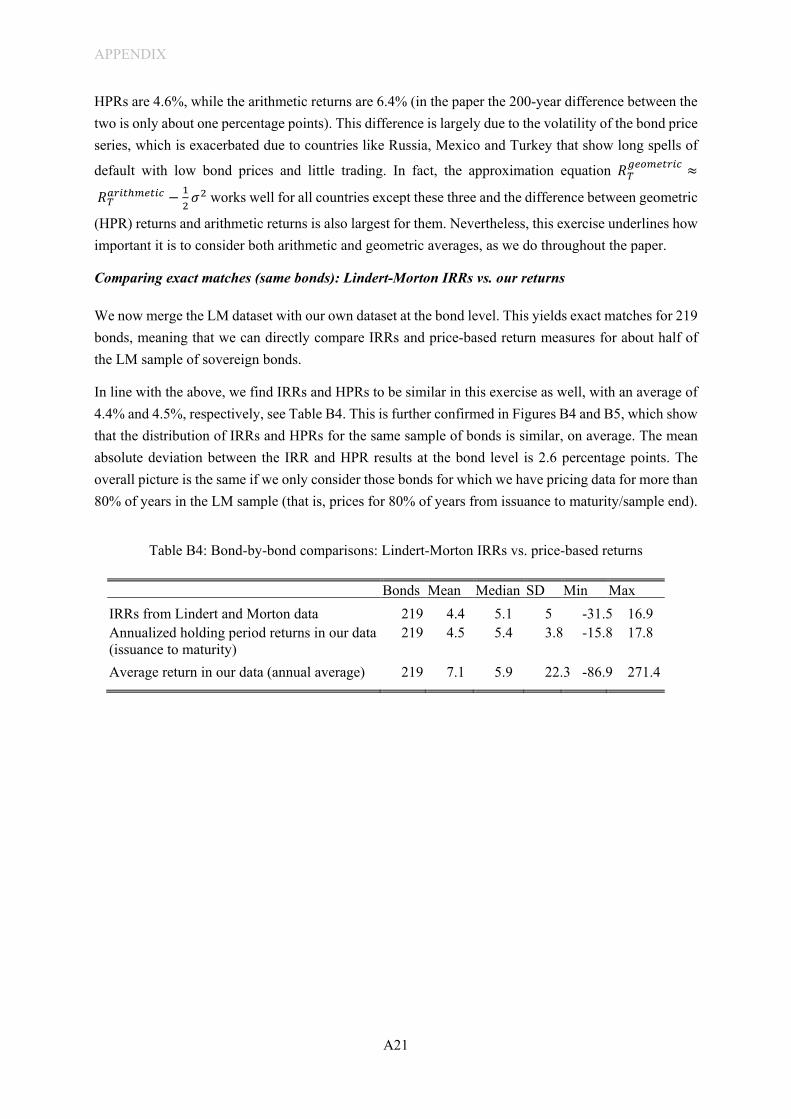
APPENDIX
A21
HPRs are 4.6%, while the arithmetic returns are 6.4% (in the paper the 200-year difference between the two is only about one percentage points). This difference is largely due to the volatility of the bond price series, which is exacerbated due to countries like Russia, Mexico and Turkey that show long spells of
default with low bond prices and little trading. In fact, the approximation equation 𝑅𝑅𝑇𝑇𝑔𝑔𝑠𝑠𝑝𝑝𝑚𝑚𝑠𝑠𝑡𝑡𝑟𝑟𝑖𝑖𝑐𝑐 ≈
𝑅𝑅𝑇𝑇𝑠𝑠𝑟𝑟𝑖𝑖𝑡𝑡ℎ𝑚𝑚𝑠𝑠𝑡𝑡𝑖𝑖𝑐𝑐 −12𝜎𝜎2 works well for all countries except these three and the difference between geometric
(HPR) returns and arithmetic returns is also largest for them. Nevertheless, this exercise underlines how important it is to consider both arithmetic and geometric averages, as we do throughout the paper.
Comparing exact matches (same bonds): Lindert-Morton IRRs vs. our returns
We now merge the LM dataset with our own dataset at the bond level. This yields exact matches for 219 bonds, meaning that we can directly compare IRRs and price-based return measures for about half of the LM sample of sovereign bonds.
In line with the above, we find IRRs and HPRs to be similar in this exercise as well, with an average of 4.4% and 4.5%, respectively, see Table B4. This is further confirmed in Figures B4 and B5, which show that the distribution of IRRs and HPRs for the same sample of bonds is similar, on average. The mean absolute deviation between the IRR and HPR results at the bond level is 2.6 percentage points. The overall picture is the same if we only consider those bonds for which we have pricing data for more than 80% of years in the LM sample (that is, prices for 80% of years from issuance to maturity/sample end).
Table B4: Bond-by-bond comparisons: Lindert-Morton IRRs vs. price-based returns
Bonds Mean Median SD Min Max IRRs from Lindert and Morton data 219 4.4 5.1 5 -31.5 16.9 Annualized holding period returns in our data (issuance to maturity)
219 4.5 5.4 3.8 -15.8 17.8
Average return in our data (annual average) 219 7.1 5.9 22.3 -86.9 271.4

APPENDIX
A22
Figure B4: Distribution of HPR and Linder-Morton IRRs, same bonds
Note: This figure shows density plots of IRRs and HPRs for the 219 bonds that are included in both the LM dataset and in our study. The H0 of unequal distributions cannot be rejected at the 1% or 5% significant level.
Figure B5: Scatter plot of LM-IRRs and HPRs, same bonds
Note: The red line represents the 45-degree line. We exclude three outlier bonds that have particularly negative IRRs (specifically, IRRs are more than 15 percentage points lower than the HPR returns), namely two Turkish bonds, and one Egyptian bond.
B3.2. Comparison to Klingen, Weder and Zettelmeyer (1970-2000)
Klingen, Weder, and Zettelmeyer (2004) provide the most comprehensive analysis of sovereign debt returns for the 1970s and 1980s, an era dominated by syndicated bank lending. Since loan-level pricing data is not available, they compute IRRs based on World Bank data on aggregate debt flows (net transfers, adjusted for losses due to default). To calculate the IRRs, they further collect data on secondary market prices on syndicated loans and bonds. This is necessary to approximate the value that investors receive at the end of the sample in 2000. Specifically, Klingen, Weder, and Zettelmeyer (2004) use the end-of-sample market prices to approximate the value of the debt stock held by investors. For the 1990s, this approach allows them to also impute short-term returns (e.g., annually or by decade) and not just holding-period-returns for the entire 1970-2000 spell.
0
.05
.1
.15
.2
.25
Den
sity
-30 -20 -10 0 10 20Return measure in %
HPRs LM IRRs
-20
-15
-10
-5
0
5
10
15
20
Nom
inal
LM
-IRR
in %
-20 -15 -10 -5 0 5 10 15 20Nominal annualized HPR in %

APPENDIX
A23
They find that, between 1970-2000, investors earned a 9% annual return, about the same as the return on US government bonds (zero risk premia). However, results vary substantially over time. In the 1970s and 1980s, annual nominal returns were typically negative, with spreads above US government bonds amounting to -5% (see Table 6 in their paper). In contrast, after 1989, sovereign debt generated double-digit nominal returns, with spreads above US Treasuries averaging 12.9% (Table 6).
To compare their results to ours, we proceed in two steps. First, we compare their average bond returns for the 1990s, which is when our and their samples overlap. Second, we add new evidence on returns in the 1980s using country-level data on syndicated loan prices and discuss the findings in the next section. Overall, we get similar results. Returns were very low in the mid-1980s but increase notably in the 1990s, as shown in the following.
To make the comparison for the 1990s as complete as possible, we gather additional data on sovereign bonds and their returns for the early 1990s, so that we cover the entire decade (1990-2000) and not just 1995-2000 (our baseline modern sample). The additional 1990-1994 data on bond prices, coupon payments, etc. was drawn from older EMBI reports as well as the morganmarkets database and was available for 10 countries (Argentina, Brazil, Chile, Colombia, Indonesia, Mexico, Philippines, Thailand, Turkey, Venezuela) while we have no data for Malaysia South Korea. 4 To compute decadal averages we use the one-year holding periods reported in Table A8 in their paper.
Table B5: Comparison of Klingen, Weder and Zettelmeyer (2004) with our returns
Mean Median SD Min Max
KWZ (2004), nominal total arithmetic returns: Nominal total returns, 1990-2000 (12 countries, Table A8 in their paper)
12.9 14.4 13.8 -7 37
Our data, nominal total arithmetic returns: With our baseline sample: 1995-2016 12.4 11.6 15.0 -22.8 38.7 With the KWZ sample, 10 countries, nominal returns:
…. Mid-1990s onwards (sample: 1995-2000) 17.7 19.1 13.3 -0.05 31.8 …. Adding data for early 1990s (sample: 1990-2000) 12.1 16.1 19.1 -31 34.2
Note: KWZ compute bond returns for the following countries: Argentina, Brazil, Chile, Colombia, Indonesia, South Korea, Malaysia, Mexico, Philippines, Thailand, Turkey, Venezuela. For the early 1990s, we collected data for 10 of these but lack data on Malaysia and South Korea. Table B5 shows the results of this comparison exercise. The main takeaway is that, for the 1990s, the average bond returns are very similar to ours, with nominal yearly returns between 12% and 16%. When collecting additional data for bank loan returns, we again find similar results to KWZ (2004), as shown in the next section.
4 KWS additionally have data for Malaysia and South Korea.

APPENDIX
A24
B4. Returns in the 1970s, 1980s and early 1990s
The developing country debt crisis of the late 1970s, 1980s and early 1990s was one of the worst periods for debtor countries and their creditors. This “lost decade”, however, is not covered in our main analysis because the 1970s and 1980s were the era of syndicated bank lending, with almost no sovereign bond issuances and, accordingly, no reliable bond price data to compute returns. To shed light on the returns during this period nevertheless we take two steps. First, we gather data from 1974-1980 and show returns for a small sample of 32 sovereign debtors that still had some bonds trading in London or New York in the mid- and end-1970s. 5 Second, we compute returns 1985-1993 using monthly syndicated loan prices. The secondary market for sovereign loans of developing countries emerged in the early 1980s, as the large commercial banks that had issued the syndicated loans started to trade them among themselves and with outside investors. Here we use the rich data collection by Sawada (2001) who combines published data by Euromoney, Salomon Brothers, Lehman Brothers, Merrill Lynch and other banks. To complement the data in the 1990s we also draw on the additional sovereign bond return data from 1990-1994 that we describe in the previous sub-section.
Table B6 summarizes the results for the different time periods between the 1970s and 1990s for which we could gather data. In line with our main analysis, we compute arithmetic average returns across observations using the portfolio of available bonds. In addition, Figure B6 shows a spliced time series of real yearly annual returns, thus combining returns on bonds (price changes and coupons) with returns on syndicated loans (price changes only, using the country-level secondary market prices collected by Sawada 2001).
Figure B6: Sovereign debt returns 1970-2000:
Combining our return series with loan price data from the 1980s and early 1990s
Note: This figure shows a spliced time series of real yearly returns. We combine our augmented return series of external sovereign bonds, shown as grey bars (price changes and coupons) with returns on eurocurrency sovereign syndicated loans, shown as red bars (price changes only). The bond returns for the 1970s and early 1980s are computed using additionally collected data from London and New York (see Table A5 above) and
5 In our main analysis we end the aggregate series in 1973 because trading volumes and bid-ask spreads show how limited the trading activity with sovereign bond was in these years, making the pricing data increasingly noisy.
-40
-20
0
20
40
60
Ann
ual r
eal r
etur
n in
%
1970 1975 1980 1985 1990 1995 2000
Total return portfolio (annual, real) Syndicated bank loan returns (annual, real)

APPENDIX
A25
then applying the same approach as in our main analysis (arithmetic yearly returns across observations). The returns on syndicated loans build on secondary market loan prices collected by Sawada (2001), which are available at a monthly level for 15 countries. Loan interest payments are not taken into account, however, also because most countries in the sample for which we have loan data were in default at the time. Since we ignore interest payments, the red bars show a lower-bound estimate of total returns on syndicated loans in those years.
We find that creditor returns, both nominal and real, were historically low in the late 1970s and 1980s, but very high in the early 1990s, which is in line with Klingen, Weder and Zettelmeyer (2004). At the height of the 1980s debt crisis, between 1986 and 1989, creditors suffered large losses on their bank loan holdings, with nominal yearly returns of -16%, while the early 1990s saw a strong recovery, as also shown in Figure B4. This is further confirmed in Figure B7.
Table B6: Creditor returns in the 1970s, 1980s and early 1990s
Nominal return Real return Mean Median SD Mean Median SD
Returns on syndicated loans (late 1980s and early 1990s)
based on secondary market loan prices from Sawada (2001) covering 15 countries 1986-1993. Yearly average arithmetic returns
Full sample by Sawada (2001):
1986-1993 (prices only) 11.1 4.4 35.4 7.3 -0.9 34.7 …. adding interest (LIBOR + 1%) 19 13.2 35.9 14.6 7.6 33.1
Late 1980s vs early 1990s only:
1986-1989 (prices only) -16 -13.7 12.9 -18.9 -15.9 12.9 1990-1993 (prices only) 38.3 35.7 28.2 33.5 31.7 28.5 Returns on sovereign bonds (1970s and early 1990s) Based on additionally collected data on sovereign bond prices of the time. Yearly average arithmetic returns.
1970s (32 countries, 106 bonds) Full decade (1970-1980) 12.4 6.0 25.6 1.5 -1.3 22.1 Late 1970s (1976-1980) 1.6 6.0 20.3 -7.6 -1.3 20.3 Early 1990s (7 countries, 22 bonds) 1990-1994 10.3 4.7 26.1 7.9 2.2 25.5
Note:
• The returns on sovereign bonds build on the same sources and methods described in the main paper, using total returns (prices and coupons). The main difference is that we collected additional data on the few remaining outstanding bonds in the 1970s, 1980s and those outstanding in the early 1990s.

APPENDIX
A26
• The returns on syndicated bank loans build on secondary market loan prices collected by Sawada
(2001), We first compute monthly price-based returns as 𝑅𝑅𝑠𝑠𝑡𝑡𝑀𝑀𝑟𝑟𝑎𝑎𝑡𝑡𝑖𝑖 = 𝑃𝑃𝑟𝑟𝑖𝑖𝑐𝑐𝑠𝑠𝑡𝑡𝑙𝑙𝑙𝑙𝑙𝑙𝑙𝑙,𝑖𝑖
𝑃𝑃𝑟𝑟𝑖𝑖𝑐𝑐𝑠𝑠𝑡𝑡−1𝑙𝑙𝑙𝑙𝑙𝑙𝑙𝑙,𝑖𝑖 − 1 for each country i
and month t and use these to compute yearly returns for each country i and year y 𝑅𝑅𝑠𝑠𝑡𝑡𝑀𝑀𝑟𝑟𝑎𝑎𝑦𝑦𝑖𝑖 = ∏ �1 + 𝑅𝑅𝑠𝑠𝑡𝑡𝑀𝑀𝑟𝑟𝑎𝑎𝑡𝑡𝑖𝑖�121 . Aggregate returns series using unweighted averages across countries for a
specific year y. • To convert nominal rates to real rates we use US inflation (see Appendix A for sources). • To estimate returns including interest we assume that the loans were paid the LIBOR rate plus 1%,
which is the spread often agreed in the Baker debt restructuring deals of the mid-1980s (see Cruces and Trebesch 2013). The (end of year) LIBOR rates used for this purpose come from the IFS (Series Code: "11160LDFZF...").
Figure B7: Syndicated loan prices, 1986-1993 by country (from Sawada 2001)
B5. Robustness checks: dissecting bond returns This section dissects the ex-post, real returns in our long-run sample of external sovereign bonds and checks the results for robustness. Specifically, we explore the role of 1) selection effects (attrition and survival bias), 2) price vs. coupon effects, 3) portfolio weighting (issue amounts vs. market capitalization) 4) the definition of serial defaulters, and 5) the inflation rate used. We also show our main summary statistics for monthly instead of yearly data.

APPENDIX
A27
B5.1. Sample composition effects (survival bias)
Survival bias is a special case of selection bias that may distort our results. As evident from Figure B3 above, our global portfolio is not balanced, as countries (and bonds) exit and enter over the 200 years span we cover. Part of the entries and exits are explained by historical events such as independence (newly founded countries start issuing debt abroad) or state break-ups (e.g., Yugoslavia), while other countries stop issuing foreign-currency bonds altogether, for example, advanced countries such as Austria, Finland or Switzerland that issued external bonds during the interwar years but moved to domestic-currency bonds since.
We explore the role of sample selection and survival bias by focusing on a subset of 15 countries for which we have more than 100 years of data and thus many decades of overlapping coverage. These countries are, in descending order of years covered: Chile (150 years of data), Russia (150), Mexico (146), Brazil (145), Argentina (137), Spain (131), Greece (128), Colombia (126), Peru (124), Portugal (114), Uruguay (114), Hungary (107), Italy (103), China (103), Australia (101).
Table B7 shows the average real, ex-post bond return for this subsample of countries with extensive coverage and compares it to that of our baseline results (full-sample global portfolio average). As can be seen, the summary statistics (average returns and their standard deviation) are very similar in the full sample and in the sample of countries with extensive coverage. This alleviates concerns that our results are biased due to survival bias.
Table B7: Survival bias: returns for countries with extensive coverage
Real, arithmetic return
Real annual, geom. return
Sharpe ratio
Annual mean
SD
Baseline result (full sample, see Table 3) 6.85 15.03 5.78 0.32
Sub-sample of 14 countries with more than 100 years of data
6.34 16.24 5.11 0.26
Note: This table compares the average returns in our full sample (baseline in the global portfolio) to those of a subgroup of countries for which we have similar coverage over more than 100 years.
B5.2. Return decomposition: coupon vs. price component
This sub-section shows that the reported total returns of our external bond portfolio can mainly be attributed to coupon payments (gains from interest) rather than to price changes (capital gains). Table B8 compares our baseline results for nominal total returns (left panel) with a price-based return measure that excludes coupon payments (right panel). Since inflation can vary substantially over time, it is more straightforward to do this decomposition with nominal returns, but the results are similar when using real returns instead.

APPENDIX
A28
Table B8: Return decomposition (nominal returns): coupon vs. price component
Total returns - nominal (prices + coupons)
Price based returns- nominal (without coupon)
Arithmetic Mean
Geometric Mean
SD Arithmetic Mean
Geometric Mean
SD
Full sample, 1815-2016, yearly 8.00 7.14 13.72 2.44 1.62 13.72 … without world wars 7.70 6.88 13.24 2.14 1.36 13.24
By era, yearly 1815-1869 6.90 5.87 14.84 1.62 0.62 14.84 1870-1914 6.18 5.91 7.45 0.69 0.42 7.45 1915-1945 7.12 6.00 16.19 1.77 0.70 16.19 1946-1973 10.15 9.19 15.12 5.83 4.93 15.12 1995-2016 12.40 11.41 14.97 4.25 3.31 14.97
Figure B8: Cumulative returns with and without coupon payments
Panel A: 1870-1940
Panel B: 1995-2016
Note: This graph shows cumulative total return indices indexed at 100 at the start of the period. We assume reinvestment of principal and interest into the country portfolio.
0
500
1,000
1,500
2,000
2,500
Cum
ulat
ive
retu
rn in
dex
(187
0=10
0)
1870 1880 1890 1900 1910 1920 1930 1940
Total returns (prices + coupon)Price-based returns only (without coupon payments)
0
200
400
600
800
Cum
ulat
ive
retu
rn in
dex
(199
5=10
0)
1995 2000 2005 2010 2015
Total returns (prices + coupon)Price-based returns only (without coupon payments)

APPENDIX
A29
Figure B9: Average bond prices across eras (year-end price averages in USD or GBP from our database )
B5.3. Alternative portfolio weights
To compute the global external sovereign bond portfolio in our main analysis, we use the issuance amount to weight each bond. Here, we show results when using alternative weighting approaches, in particular when using (i) market capitalization of the bonds and (ii) equal weights for each bond. Historically the time series for market capitalization is noisy for a number of bonds for which we lack details on exact monthly amortization. We therefore approximate market capitalization by multiplying the issuance amount of each bond with its current monthly secondary market price. In the modern sample, monthly market capitalization per bond is taken from the JP Morgan EMBI database.
Table B9 shows that the average return in the full sample increases slightly when using market capitalization (0.63 percentage points higher real return) and somewhat more when weighting each bond equally (0.43 percentage points higher real returns). The same is true for the modern (1995-2016) sample. The differences are larger when we use our proxy for market capitalization lagged by one period (in t-1), with lower average returns, particularly in the interwar and post-WW2 sub-samples. However, as explained above, we do lack data on actual amounts outstanding in history, making the historical value-based averages noisy. In sum, our baseline weighting approach (by issuance amounts) is a conservative choice with the main advantage that it can be applied consistently over the full 200-year sample.
0
20
40
60
80
100
120
1820 1830 1840 1850 1860 1870
1815-1869
0
20
40
60
80
100
120
1870 1880 1890 1900 1910
1870-1914
0
20
40
60
80
100
120
1915 1920 1925 1930 1935 1940 1945
1915-1945
0
20
40
60
80
100
120
1945 1950 1955 1960 1965 1970 1975
1946-1973
0
20
40
60
80
100
120
1995 2000 2005 2010 2015
1995-2016
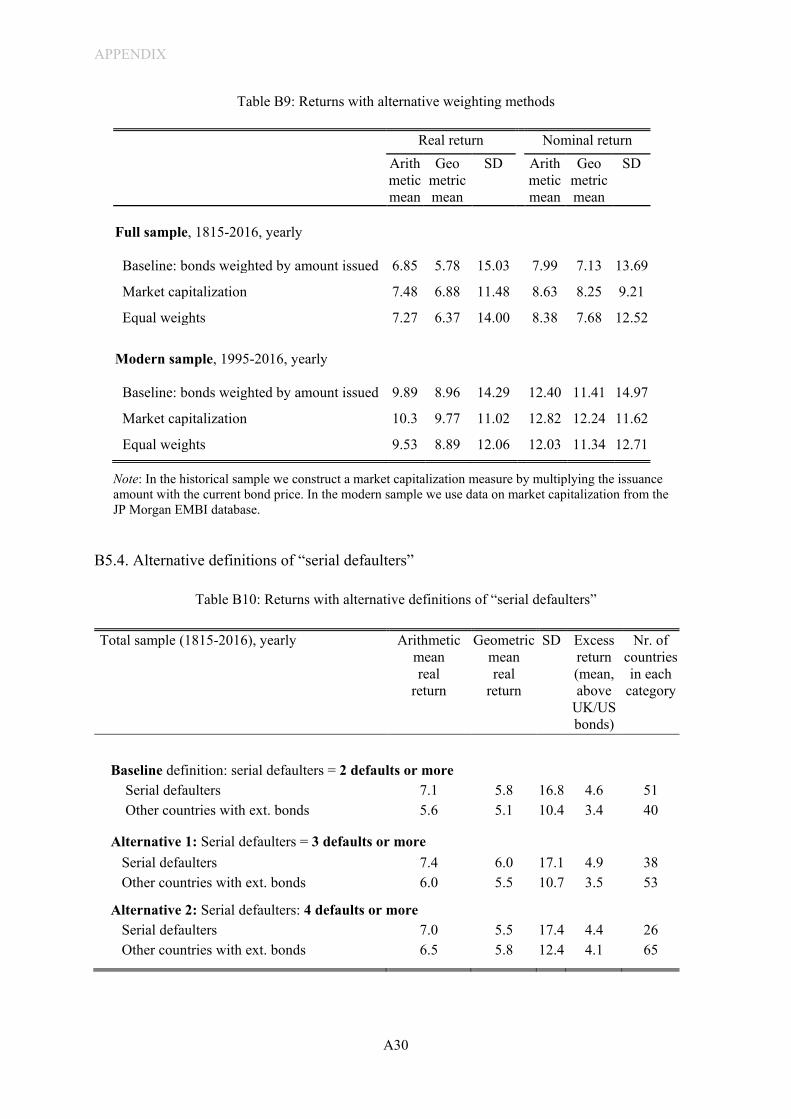
APPENDIX
A30
Table B9: Returns with alternative weighting methods
Real return Nominal return
Arithmetic mean
Geo metric mean
SD Arithmetic mean
Geo metric mean
SD
Full sample, 1815-2016, yearly Baseline: bonds weighted by amount issued 6.85 5.78 15.03 7.99 7.13 13.69
Market capitalization 7.48 6.88 11.48 8.63 8.25 9.21
Equal weights
7.27 6.37 14.00 8.38 7.68 12.52
Modern sample, 1995-2016, yearly Baseline: bonds weighted by amount issued
9.89 8.96 14.29 12.40 11.41 14.97
Market capitalization
10.3 9.77 11.02 12.82 12.24 11.62
Equal weights
9.53 8.89 12.06 12.03 11.34 12.71 Note: In the historical sample we construct a market capitalization measure by multiplying the issuance amount with the current bond price. In the modern sample we use data on market capitalization from the JP Morgan EMBI database.
B5.4. Alternative definitions of “serial defaulters”
Table B10: Returns with alternative definitions of “serial defaulters”
Total sample (1815-2016), yearly Arithmetic mean real
return
Geometric mean real
return
SD Excess return (mean, above
UK/US bonds)
Nr. of countries in each
category
Baseline definition: serial defaulters = 2 defaults or more Serial defaulters 7.1 5.8 16.8 4.6 51 Other countries with ext. bonds 5.6 5.1 10.4 3.4 40
Alternative 1: Serial defaulters = 3 defaults or more Serial defaulters 7.4 6.0 17.1 4.9 38 Other countries with ext. bonds 6.0 5.5 10.7 3.5 53
Alternative 2: Serial defaulters: 4 defaults or more Serial defaulters 7.0 5.5 17.4 4.4 26 Other countries with ext. bonds 6.5 5.8 12.4 4.1 65

APPENDIX
A31
For the main analysis we define “serial defaulters” as those countries that have defaulted two times or more. Here, we show that the results are similar when using a stricter definition, that is, with a cut-off at 3 or 4 defaults instead of 2. Table B10 shows that the number of countries in the “serial default” bucket drops quickly when moving to “three or more default” or “four or more defaults”. In each case, however, the returns of serial defaulters remain above those of the comparison group.
B5.5. Inflation expectations
Table B11: Real returns: the role of inflation
Real arithmetic return
Real geometric return, yearly mean Yearly
mean SD
Total sample Using realized inflation in year t 6.85 15.03 5.78 Using inflation in year t+1 6.66 14.12 5.73 Historical sample, 1818-1973 Using realized inflation in year t 6.40 15.13 5.33 Using inflation in year t+1 6.18 14.07 5.26 Modern sample, 1995-2016 Using realized inflation in year t 9.89 14.29 8.96 Using inflation in year t+1 9.94 14.46 8.98
Note: This table shows summary statistics for the global sovereign bond portfolio when nominal returns are adjusted using current inflation in year t and, alternatively, using inflation in year t+1.
Our baseline results are expressed in real terms, using long-run data on consumer price inflation in the US and the UK (see Appendix A). Real returns compensate investors for the realized inflation in year t, but nominal returns will also reflect expected future inflation rates in t+1, t+2, etc. Using current realized inflation rates may thus bias the results. To account for this possibility, we check the robustness of our return estimates when using inflation rates 12 months ahead.

APPENDIX
A32
B5.6. Monthly vs. yearly summary statistics
Table B12 adds to the main tables in Section 4 in the main paper by showing all main statistics when using monthly vs. yearly data.
Table B12: Monthly vs. yearly summary statistics
Mean real
returns
Median real
returns
SD Skew-ness
Kur-tosis
Benchmark: UK/US bills
Benchmark: UK/US bonds
Excess return
Sharpe ratio
Adj. Sharpe ratio
Excess return
Sharpe ratio
Adj. Sharpe ratio
Yearly
Full sample, 1815-2016, yearly
6.85 6.58 15.03 0.26 4.09 4.98 0.36 0.40 4.35 0.32 0.35
Modern sample, 1995-2016, yearly
9.89 8.82 14.29 -0.26 3.1 9.52 0.66 0.68 6.26 0.33 0.45
Monthly
Full sample, 1815-2016, monthly
0.54 0.48 3.73 0.03 12.63 0.38 0.10 0.45 0.35 0.10 0.41
Modern sample, 1995-2016, monthly
0.46 0.41 3.78 0.16 11.86 0.30 0.08 0.38 0.28 0.08 0.36
B6. Bond liquidity: additional evidence
This section complements Section 3.5 in the main paper by showing average returns depending on the liquidity of the bonds, as proxied by bid-ask spreads. We construct liquidity buckets by grouping each bond into one of the five quintiles of the distribution of bid-ask spreads, with the first group having the lowest average bid-ask spread (most liquid group). The last two columns show the p-value from a simple t-test for difference in group means, comparing each liquidity bucket to the most liquid one.
As can be seen, average real returns are significantly higher for less liquid bonds (with higher bid-ask spreads). The difference between the most liquid and the least liquid group is almost two percentage points in the full sample and statistically significant for the fourth and fifth quintile.

APPENDIX
A33
Table B13: Bond returns and bond liquidity liquidity buckets based on bid-ask spreads
Bid-ask spread Diff bid-ask Real return
Excess return (above US/UK
bonds)
Difference to most liquid,
p-value of t-test
Mean Median Mean Median Mean Median Mean Median Excess return
Real return
Total sample 1870-2016 1 (most liquid quintile) 0.47 0.36 0.43 0.38 0.49 0.45 0.30 0.35 2 1.01 0.87 0.97 1.00 0.52 0.42 0.35 0.33 0.118 0.336 3 1.53 1.14 1.33 1.00 0.47 0.41 0.29 0.35 0.829 0.920 4 2.34 1.86 1.70 1.00 0.63 0.47 0.45 0.47 0.000 0.000 5 (least liquid quintile) 5.40 2.53 2.23 1.75 0.61 0.34 0.43 0.39 0.955 0.060 Historical sample (1815-1973) 1 (most liquid) 0.50 0.00 0.43 0.00 0.49 0.49 0.32 0.39 2 1.21 1.09 1.12 1.00 0.48 0.41 0.35 0.33 0.298 0.945 3 1.85 1.94 1.54 2.00 0.41 0.38 0.26 0.33 0.451 0.303 4 3.01 2.38 2.03 2.00 0.57 0.40 0.41 0.42 0.007 0.007 5 (least liquid) 7.88 4.60 2.75 2.00 0.49 0.29 0.37 0.30 0.175 0.008 Modern sample (1995-2016) 1 (most liquid) 0.40 0.40 0.45 0.50 0.50 0.35 0.26 0.26 2 0.60 0.58 0.67 0.65 0.60 0.50 0.34 0.33 0.094 0.024 3 0.78 0.74 0.82 0.75 0.61 0.60 0.37 0.39 0.053 0.033 4 1.01 0.93 0.99 1.00 0.76 0.75 0.51 0.59 0.000 0.000 5 (least liquid) 1.66 1.30 1.35 1.00 0.75 0.69 0.49 0.57 0.016 0.006
B7. CAPM results This section implements a simple Fama MacBeth (1973) CAP- model for external sovereign bonds along the lines of Bordo and Rockoff (1996) and Borri and Verdelhan (2015). In a first stage we estimate the market betas 𝛽𝛽𝑖𝑖 for each country-portfolio as follows:
𝑅𝑅𝑡𝑡,𝑖𝑖 = 𝛼𝛼𝑖𝑖 + 𝛽𝛽𝑖𝑖′𝑅𝑅𝑡𝑡,𝑚𝑚 + 𝜖𝜖𝑡𝑡,𝑖𝑖 (B7)
where 𝑅𝑅𝑡𝑡,𝑚𝑚is the return on a world market portfolio, i denotes the country portfolio (or global portfolio),
t is the month and 𝜖𝜖𝑡𝑡𝑖𝑖 is an error term. As market portfolio we use a spliced series of UK stock returns until 1918 (FTSE index), and US equity returns after 1918 (S&P 500 index), see Appendix A for sources. The betas thus capture the covariance between the bond returns and US/UK equity returns, that is, the sensitivity of external bond returns to US/UK stock market movements.

APPENDIX
A34
In the second stage, we run cross-sectional regressions (across portfolios) on the estimated betas �̂�𝛽𝑖𝑖 from the first regression to estimate the market risk premium, as follows:
𝐸𝐸[𝑅𝑅𝑡𝑡] = 𝜆𝜆𝑡𝑡�̂�𝛽𝑖𝑖 + 𝛼𝛼𝑖𝑖𝑡𝑡
(B8)
where 𝐸𝐸[𝑅𝑅𝑡𝑡] is the expected monthly return for the respective portfolio i in month t. To compute the
market price of risk, we compute the mean of all Lambda 𝜆𝜆𝑡𝑡, that is, �̂�𝜆 = ∑ 𝜆𝜆𝑡𝑡�𝑇𝑇𝑖𝑖=1 , which captures the
average risk premium on the world market portfolio. The alphas 𝛼𝛼𝑖𝑖𝑡𝑡 are the pricing errors, capturing the part of the return 𝑅𝑅𝑡𝑡 unexplained by �̂�𝛽𝑖𝑖.
For the analysis, we focus on three subsamples with broad country coverage, (i) the first era of globalization 1870-1913, (ii) the interwar period 1919-1939, and (iii) the modern sample 1995- 2016.
First stage: Estimated betas
Figure B9 shows a scatter plot of the estimated betas �̂�𝛽𝑖𝑖 (eq. B7) and average monthly excess returns for each country. Two insights emerge. First, higher betas are associated with higher average excess returns, but only in the pre-WW1 and the modern bond era. Second, high beta countries also show higher excess returns, on average.
Figure B9: Estimated betas and average excess returns by country
AUSBELCAN
DNK
ITAJPN
NZLNORSWE
ARG
BRABGR
CHLCHN
COL
CRI
DOM ECUEGY
GRCGTM
HNDHUN
MEXNICPRY
PER
PRT
ROU
RUS
ESP
TURURY
VEN
Betas:Mean: 0.14Median: 0.10Min: -1.06Max: 0.94
-0.4
-0.2
0.0
0.2
0.4
0.6
Rea
lized
ave
rage
mon
thly
exc
ess r
etur
ns in
%
-1.0 -0.5 0.0 0.5 1.0Country-betas
Serial defaulters All others
1870-1913
AUSBEL
CANDNK
FINFRA
IRL ITAJPN
NZL NOR
SWETHA
ARG
AUT
BRA
BGRCHL
CHNCOL
CRICUB
DOM
EGY
SLV
DEU
GRC
GTMHTI
HND HUNMEX
NIC PANPRY
PERPOL
PRT
ROUZAFESP
TUR
URYVEN
SRB
Betas:Mean: 0.21Median: 0.16Min: -0.02Max: 0.81
-0.4
-0.2
0.0
0.2
0.4
0.6
0.8
Rea
lized
ave
rage
mon
thly
exc
ess r
etur
ns in
%
0.0 0.2 0.4 0.6 0.8Country-betas
Serial defaulters All others
1919-1939
BLR
HRV
GEO
LBN LTUMYS NAM
PHLKOR
THAVNM
ARG
BLZ
BRABGR
CHLCHN
COL
CIV
DOM
ECU
EGYSLV
GABGHA
HUNIDN
IRQJAM
MEX MAR
NGAPAK
PANPER
POL
RUSSEN
ZAF
LKATURUKR
URY
VEN
SRB
Betas:Mean: 0.36Median: 0.37Min: -0.10Max: 0.78
0.0
0.5
1.0
1.5
Rea
lized
ave
rage
mon
thly
exc
ess r
etur
ns in
%
-0.2 0.0 0.2 0.4 0.6 0.8Country-betas
Serial defaulters All others
1995-2016

APPENDIX
A35
Table B14 further shows estimated betas in the aggregate portfolio, using all countries as well as the sub-samples of serial defaulters and no/one-time defaulters as defined above. The estimated beta is highest in the modern sample, suggesting that global factors (UK/US equity returns) play a more important role today (consistent with Mauro, Sussman, and Yafeh 2002). The beta is also higher for serial defaulters.
Table B14: Estimated betas for the aggregate portfolio
Coefficient R2 Months covered Intercept Beta
1870-1913
Global Portfolio 0.002** 0.115** 0.006 588 (0.001) (0.054)
Serial defaulter 0.003** 0.136** 0.007 588 (0.001) (0.062)
Non-defaulters 0.002 0.009** 0.000 576 (0.001) (0.058)
1919-1939
Global Portfolio -0.001** 0.232 0.262 252 (0.002) (0.037)
Serial defaulter -0.002** 0.313 0.254 252 (0.002) (0.047)
Non-defaulters 0.002** 0.096* 0.167 252 (0.001) (0.028)
1995-2016
Global Portfolio 0.005** 0.486** 0.294 252 (0.002) (0.094)
Serial defaulter 0.005** 0.503** 0.299 252 (0.002) (0.094)
Non-defaulters 0.006** 0.173*** 0.14 240 (0.001) (0.047)
Second stage: Predicted returns
Figure B10 plots realized average excess returns against predicted average excess returns, with the latter
being computed as the product of the OLS estimates of �̂�𝛽𝑖𝑖 and �̂�𝜆. In the modern sample (1995-2016), a single risk factor (US equity returns) explains a large share of the variation across countries. This is less the case in the historical samples. Alphas are larger in the historical samples, especially in the interwar

APPENDIX
A36
period, but comparatively small in the modern sample. Our results for 1995-2016 are similar to those of Borri and Verdelhan (2015).
Figure B10: Realized and predicted excess returns
ARG
AUSBELBRA
BGR
CAN
CHLCHN
COLCRI
DNK
DOM ECUEGY
GRCGTM
HNDHUNITAJPN
MEX
NZL
NIC
NOR
PRY
PER
PRT
ROU
RUS
ESP
SWE
TURURY
VEN
Alphas:Mean: 0.20Median: 0.19Min: -0.48Max: 1.12-0.5
0.0
0.5
1.0
Rea
lized
ave
rage
mon
thly
exc
ess r
etur
n (in
%)
-0.5 0.0 0.5 1.0Predicted average
monthly excess return (in %)
1870-1913
ARG
AUS
AUT
BEL
BRA
BGRCAN CHL
CHN
COL
CRICUB
DNK
DOM
EGY
SLVFINFRA
DEU
GRC
GTMHTI
HND HUNIRL
ITA
JPN
MEX
NZL
NIC
NOR
PANPRY
PERPOL
PRT
ROUZAFESP
SWE
THA
TUR
URYVEN
SRB
Alphas:Mean: 0.16Median: 0.23Min: -0.66Max: 0.57-0.4
-0.2
0.0
0.2
0.4
0.6
Rea
lized
ave
rage
mon
thly
exc
ess r
etur
n (in
%)
-0.4 -0.2 0.0 0.2 0.4 0.6 0.8Predicted average
monthly excess return (in %)
1919-1939
ARGBLR
BLZ
BRABGR
CHLCHN
COL
CIV
HRVDOM
ECU
EGYSLV
GAB
GEO
GHA
HUNIDN
IRQJAM
LBN LTUMYS
MEX MAR
NAM
NGAPAK
PANPERPHL
POL
RUSSEN
ZAFKOR
LKA
THA
TURUKR
URY
VEN
VNMSRB
Alphas:Mean: 0.09Median: 0.10Min: -0.53Max: 1.03-0.5
0.0
0.5
1.0
1.5
Rea
lized
ave
rage
mon
thly
exc
ess r
etur
n (in
%)
-0.5 0.0 0.5 1.0 1.5Predicted average
monthly excess return (in %)
1995-2016

APPENDIX
A37
B8. Case studies: total returns around sovereign default
This section shows 11 case studies on total cumulative real returns around spells of sovereign default. The indices are indexed at 100 at the start of the period (January of the year). We assume reinvestment of principal and interest into the country portfolio. Default episodes are shaded in grey.
Argentina 1870-1910: cumulative total return index
Argentina 1994-2016: cumulative total return index
0
500
1,000
1,500
2,000
Cum
ulat
ive
tota
l ret
urn
inde
x
1870 1880 1890 1900 1910
0
100
200
300
Cum
ulat
ive
tota
l ret
urn
inde
x
1995 2000 2005 2010 2015

APPENDIX
A38
Brazil 1925-1950: cumulative total return index
Chile 1900-1960: cumulative total return index
Colombia 1915-1960: cumulative total return index
0
200
400
600
800
Cum
ulat
ive
tota
l ret
urn
inde
x
1925 1930 1935 1940 1945 1950
0
100
200
300
400
Cum
ulat
ive
tota
l ret
urn
inde
x
1900 1910 1920 1930 1940 1950 1960
0
200
400
600
800
Cum
ulat
ive
tota
l ret
urn
inde
x
1920 1930 1940 1950 1960

APPENDIX
A39
Ecuador 1993-2016: cumulative total return index
Germany 1926-1975: cumulative total return index
Italy 1900-1970: cumulative total return index
0
200
400
600
Cum
ulat
ive
tota
l ret
urn
inde
x
1995 2000 2005 2010 2015
0
300
600
900
1200
Cum
ulat
ive
tota
l ret
urn
inde
x
1925 1934 1943 1952 1961 1970
0
200
400
600
800
Cum
ulat
ive
tota
l ret
urn
inde
x
1900 1910 1920 1930 1940 1950 1960 1970

APPENDIX
A40
Mexico 1870-1930: cumulative total return index
Russia/Soviet Union 1869-1970: cumulative total return index
Russia 1995-2016: cumulative total return index
Note: Russia was in default on Soviet-era debt since the early 1990s. The government also defaulted on its newly issued bonds in August 1998.
0
500
1,000
1,500
Cum
ulat
ive
tota
l ret
urn
inde
x
1870 1880 1890 1900 1910 1920 1930
0
500
1,000
Cum
ulat
ive
tota
l ret
urn
inde
x
1870 1895 1920 1945 1970
0
100
200
300
Cum
ulat
ive
tota
l ret
urn
inde
x
1997 2000 2003 2006 2009 2012 2015

APPENDIX
A41
References Appendix B (those not cited in the main paper)
Bordo, Michael D. and Hugh Rockoff (1996). The Gold Standard as a “Good Housekeeping Seal of
Approval”. The Journal of Economic History, 56(2), 389-428.
Borri, Nicola and Adrien Verdelhan (2015). Sovereign Risk Premia. Mimeo.
Fama, Eugene F. and James D. MacBeth (1973). Risk, Return, and Equilibrium: Empirical Tests.
Journal of Political Economy, 81 (3), 607–636.
Sawada, Yasuyuki (2001). Secondary Market Efficiency for LDC Bank Loans and International
Private Lending, 1985-1993," Journal of International Money and Finance, 20(4), 549-562.

APPENDIX
A42
Appendix C: Debt restructurings and haircuts
C1. Sample and data sources on restructurings
This Appendix describes our approach to identify sovereign debt restructurings in history, in order to complement and extend the sample compiled by Cruces and Trebesch (2013) and Fang, Schumacher, and Trebesch (2020), which cover recent decades only. For the historical period, we draw on a large body of archival and other sources which we use to conduct a census of distressed sovereign debt restructurings with foreign commercial creditors since 1815. Before 1970, we only identify bond restructurings and not a single new bank debt restructuring.
C1.1. Case selection
Following Cruces and Trebesch (2013), we use five criteria to select cases:
- First, we focus on defaults and restructurings on sovereign debt, meaning on bonds or loans owed by a country’s central government, but not on debt of local or regional governments.
- Second, we include only distressed debt exchanges, defined as restructurings of bonds (or bank loans) at less favorable terms than the original bond (loan). We thereby follow the standard definition of distressed restructurings by rating agencies such as Standard and Poor’s (2006) or Moody’s (2012). Restructurings that are part of routine sovereign liability management such as debt swaps and buybacks in normal times are disregarded.
- Third, we include restructurings of medium and long-term debt. We do not include short-term agreements such as 3-month debt rollovers or deals that provide short-term bridge financing or maturity extensions of less than one year. However, we do include restructurings in which short-term debt is transformed into medium- or long-term debt, as was the case in Mexico’s restructurings of the 1920s and a few others.
- Fourth, we focus on restructurings of privately held, foreign-currency debt, meaning external bonds or loans, which are typically held by foreign commercial creditors. We do not take into account defaults on private-to-private, or public-to-public debt, that is, no debt exchanges of official (bilateral and multilateral) creditors such as the restructuring of public war debts in the wake of WW1 and WW2 (see Reinhart and Trebesch [2016] on these cases). Restructurings of domestic bonds are excluded, also because, for most of the 19th and 20th centuries, domestic-currency debt was predominantly held by domestic creditors. In our historical sample, there are only very few defaults and restructurings of domestic currency bonds that had been marketed and/or issued in London and/or New York and were therefore almost exclusively held by foreigners (these are Brazil 1898, Russia 1917, Mexico 1922, 1925 and 1942, Austria 1952, and Germany 1953). Following the rationale of Sturzenegger and Zettelmeyer (2008) and Cruces and Trebesch (2013) we do include these quasi-foreign debt restructurings. However, the summary statistics and overall picture are essentially the same if we drop them.

APPENDIX
A43
- Fifth, we include only restructurings that are implemented. Interim agreements that were never completed are disregarded, such as the case of El Salvador 1922, where the parliament voted against the agreement, or Bulgaria in 1948, where the agreement with creditors was never legally recognized by the government. In addition, we disregard temporary deals that had the sole purpose of bridging the time until a permanent settlement and debt exchange (these preliminary agreements were particularly frequent in the 1930s and 1940s).
C1.2. Sample of restructurings
This subsection explains how we get to our final sample of 313 sovereign debt restructurings since 1815.
We start with the modern part of the sample (1970-2013) and use data on 187 restructuring events
covered in the most recent update of Cruces and Trebesch (2013). We add to this the recent
restructurings in Grenada 2015 and Ukraine 2015 which are covered by Fang, Schumacher, and
Trebesch (2020).
In the historical sample, we identify 175 sovereign debt restructurings (see full list in Appendix C3
below). Of these, 167 were implemented in the period 1815 to 1970 plus 12 that occurred after 1970 but
were not included in the sample of Cruces and Trebesch (2013). 6 Out of the 175 newly identified deals,
we could gather sufficiently rich information to estimate haircuts for all but 10 deals 7, so that the
historical sample of haircut estimates added here comprises 169 cases in 43 countries. All of these 169
historical cases were restructurings of sovereign bonds, while no loan debt restructurings could be
identified pre-1970. This confirms that external borrowing by sovereigns almost exclusively took the
form of bonded debt in the pre-WW2 era, in contrast to the 1980s and early to mid-1990s, when
restructurings mostly involve syndicated bank loans held by foreign commercial banks. Also note that,
in the historical sample, we drop 63 restructurings that did not fulfill our case selection criteria. More
specifically, we drop 23 cases that were never implemented, as well as 64 agreements that were only
temporary or focused on short-term debt and rollovers. In addition, we identified 10 default spells that
6 The 12 post-1970 restructurings which Cruces and Trebesch (2013) had missed were all long-delayed historical cases that go back to defaults of the 1930s. Except Zimbabwe 1980, they all involve Communist countries that had refused to negotiate or settle their debts with foreign bondholders for decades: Hungary 1975 (American bondholders), Poland 1975 (American bondholders), Romania 1975 (American bondholders), Poland/Danzig 1976 (American and British bondholders), Romania 1976 (British bondholders), Bulgaria 1979 (American bondholders), Czechoslovakia 1986 (American bondholders), Russia 1986 (British bondholders), Bulgaria 1987 (British bondholders), China 1987 (British bondholders) and Russia 1997 (French bondholders). 7 The 10 cases for which we lack sufficient information are Austria 1816, Russia 1839, Tunisia 1870, Austria 1871, Schleswig-Holstein 1850, and Morocco 1904 as well as five smaller cases that only affected parts of the debt, namely Poland 1949 (side-deal with Swiss bondholders), Hungary 1950 (side-deal with Dutch bondholders), Hungary 1951 (side-deal with Swedish Bondholders), and Yugoslavia 1959 (side-deal with Swiss Bondholders).

APPENDIX
A44
were resolved without a restructuring, that is, defaults cured with a debt exchange. 8 For these events, it
is therefore not possible to calculate a haircut.
In a first step, we thus combine 189 restructurings for the modern sample (187 in Cruces and Trebesch
[2013], plus 2 from 2015 from Fang, Schumacher, and Trebesch 2020) with 169 newly coded historical
ones, resulting in a total of 358 individual sovereign debt restructuring events over 200 years. Figure C1
shows the respective timelines on a country level. These 358 individual restructurings, however,
constitute an upper bound and need to be consolidated to avoid double counting. In particular, the sample
includes 78 cases in which the same default results in more than one restructuring, mostly because of
selective restructurings with different creditor groups (e.g., USD vs. GBP currency bonds). For brevity,
we use the modern name of a country in case of country mergers or break-ups (e.g., “Germany” not
“Germany-Prussia”).
As can be seen from Figure C1 some countries witness multiple restructurings within just a few years.
Take the example of Brazil, which declared a full debt moratorium in October 1931. After lengthy
negotiations, Brazil restructured its USD and GBP bonds in November 1943, but it took three more
years, until 1946, to settle its few outstanding French Franc bonds. We merge such multiple
restructurings of the same default into one event so that each spell receives just one haircut estimate.
Specifically, to compute haircuts across multiple deals of the same default, we calculate a weighted
average haircut using amounts restructured in each deal (converted to US dollar values). To date the
merged deals, we use the main agreement, meaning that restructuring in which the largest portion of the
defaulted debt was exchanged. In the Brazil example above, we compute an average haircut of the 1943
and 1946 agreements and assign the year 1943. This is because the bulk of Brazilian debt was to US and
UK creditors, while the French agreement of 1946 was widely seen as a side deal.
Overall, we identify 78 spells with multiple restructurings (28 in the modern sample and 50 in the
historical sample) and these are merged into 33 cases (45 cases less). The final, lower-bound sample
used in the analysis therefore drops to 313 external sovereign debt restructurings in 91 countries.
8 These include the temporary sinking fund suspensions by Colombia between 07/1915 and 06/1916, by Paraguay between 07/1914 and 12/1915, as well as Uruguay between 1915 and 08/1921. Another seven cases originated in the default and break-up of the Ottoman Empire (for details see the section on country break-ups below). Four countries, namely Iraq (1934), Italy (1932), Palestine (1928) and Syria and Lebanon (1933) eventually repaid their share of old Ottoman debt without a restructuring (year of repayment in parentheses). In contrast, the debt apportioned to Albania, Saudi Arabia (formerly Nedid and Hedjaz), and Yemen remained unresolved, that is, no payment could be identified until 2015.
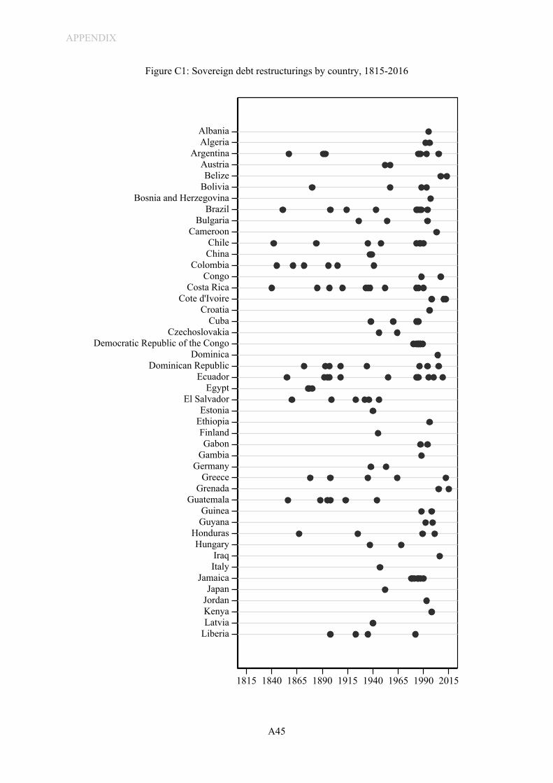
APPENDIX
A45
Figure C1: Sovereign debt restructurings by country, 1815-2016
AlbaniaAlgeria
ArgentinaAustriaBelize
BoliviaBosnia and Herzegovina
BrazilBulgaria
CameroonChileChina
ColombiaCongo
Costa RicaCote d'Ivoire
CroatiaCuba
CzechoslovakiaDemocratic Republic of the Congo
DominicaDominican Republic
EcuadorEgypt
El SalvadorEstonia
EthiopiaFinlandGabon
GambiaGermany
GreeceGrenada
GuatemalaGuineaGuyana
HondurasHungary
IraqItaly
JamaicaJapan
JordanKenyaLatvia
Liberia
1815 1840 1865 1890 1915 1940 1965 1990 2015

APPENDIX
A46
Figure C1 (continued): Sovereign debt restructurings by country, 1815-2016
Note: For brevity, in case of country mergers or country break-ups, we use the name of the new country and omit the historical name (e.g., “Germany” instead of “Germany-Prussia”, “Yugoslavia” instead of “Serbia”, “Turkey” instead of “Ottoman Empire”).
LiberiaLithuania
MacedoniaMadagascar
MalawiMauritania
MexicoMoldovaMorocco
MozambiqueNicaragua
NigerNigeria
PakistanPanama
ParaguayPeru
PhilippinesPoland
PortugalRomania
RussiaSaint Kitts and Nevis
Sao Tome and PrincipeSenegal
Serbia and MontenegroSeychelles
Sierra LeoneSlovenia
South AfricaSpainSudan
TanzaniaThailand
TogoTrinidad and Tobago
TurkeyUgandaUkraine
UruguayVenezuela
VietnamYemen
YugoslaviaZambia
Zimbabwe
1815 1835 1855 1875 1895 1915 1935 1955 1975 1995 2015
APPENDIX
A47
C1.3. Data sources on restructurings
This section describes the data sources behind our historical sovereign debt restructuring and haircut archive. On each restructuring, we collected data on the default and renegotiation dates (start, interim agreements, and debt exchange), as well as at the bonds involved and their contractual terms such as the issue prices, the maturity, coupon rates, the repayment terms (grace period, amortization scheme), and the bond amounts (face value, amounts outstanding, nominal debt reductions).
Our starting point was the ground-breaking work of Suter (1990) and Stamm (1987), who provide a documentation of historical debt restructurings from 1820 to 1975. We also rely on Reinhart and Rogoff (2009), who document the start and end dates of historical default episodes. Unfortunately, however, these sources lack details on the restructuring terms and the bonds involved, so that it is not possible to estimate haircuts and to systematically compare old and new instruments in each exchange.
We therefore embarked on an extensive data-gathering exercise using a variety of sources. In a nutshell, we used every piece of information we could find and then gather and compare the key details on the restructurings and bonds involved across each source available. This allowed us to reduce mistakes, detect contradictory information, and thereby generate a more reliable final dataset.
Most importantly, we rely on the annual reports published by creditor organizations representing the bondholders who were affected by the sovereign’s default: the Foreign Bondholders (CFB) (1876-1944, 1945-1986), the Foreign Bondholders Protective Council (FBPC) (1934-1940, 1945-1950, 1953-1964/67), the Association Belge pour la Défense des Détenteurs de Fonds Publics (1898-1915), and the French Association Nationale des Porteurs Franҫais de Valeurs Mobiliéres (1936-1945, 1948-1974, 1987-1988, 1996). The reports provide very rich details on past defaults and restructurings and were our most valuable source.
To cross-check the information by the creditor committees and to fill gaps, additional sources were consulted, in particular investor reports such as Fenn’s Compendium of the English and Foreign Funds (1837-1838, 1855, 1857, 1863, 1867, 1869, 1874, 1876, 1883, 1889, 1893), Fortune’s Epitome of the Stock and Public Funds (1800, 1810, 1820, 1824, 1826, 1833, 1838-1839, 1850-1851, 1856), Kimber's Records on Government Debts and other Foreign Securities (1918, 1919, 1922, 1934), Moody's Manuals on Foreign and American Government Securities (yearly 1920-1960), and the Stock Exchange Yearbooks (1877-1878, 1880-1881, 1883-1888, 1890, 1894-1895, 1897, 1899-1901, 1905, 1907-1916, 1919-1920, 1925). Occasionally, we also relied on academic case studies, communiques of the creditor organizations, official gazettes of the debtor country, or press articles.
Table C1 provides an overview of the data sources used for our historical sample since 1815. For almost all historical restructurings (157 cases out of 169), we had at least two sources of information with details on the restructuring terms. As can be seen, the British Corporation of Foreign Bondholders covered almost all cases included in our historical dataset.

APPENDIX
A48
Table C1: Overview of sources used (historical sample since 1815)
C1.4. Data quality index In order to assess the quality of the information we gathered, we construct a data quality index for our historical sample, following the approach in Cruces and Trebesch (2013). The index is additive and consists of five binary indicators, thus ranging from a maximum of 5 (very good data availability) to 0 (very restricted data availability). The five indicators are:
1. Knowledge of the main contractual terms of the old restructured debt. This criterion is fulfilled if we have details on restructured amounts, on which parts had fallen due, as well as on the maturity period, redemption schedule and coupons of the old debt.
2. Knowledge of the key characteristics of the new debt. This is fulfilled if we have details on the type of debts and the amounts restructured, as well as on the maturity period, the repayment/amortization schedule, and the interest rates of the new debts.
3. Whether the terms above are available by instrument, that is, bond-by-bond. 4. Full consistency across the available sources. This is fulfilled if there is no contradictory
information with regard to date, amounts, interest rates or repayment schedules. 5. Knowledge of when the restructuring is implemented. This is fulfilled if we know the exact
month of the agreement and whether a deal was ultimately implemented or not (this is the case for all restructurings in the historical sample).
Table C2 shows the distribution of the data quality index for all newly identified sovereign debt restructurings since 1815 (in 20-year intervals). This table also includes cases for which we could not gather enough details to compute haircuts, that is, the 10 cases for which data coverage is insufficient and which are therefore not included in our final sample. Indeed, the data quality index for these excluded countries is particularly low (1 on our index scale).
Sources Restructurings covered
Corporation of Foreign Bondholders (UK creditors) 146Suter (1990) and Stamm (1988) 121Foreign Bondholder Protective Council (US creditors) 65Moody's Manuals 44Fenn's Compendium 39London Stock Exchange Yearbook 30Association Belge pour le Détenteurs de Fonds Publics 25Fortune's Epitome 21Kimber's Records 21Association Nationale des Porteurs Franςais de Valeurs Mobiliéres 18Other Sources 34

APPENDIX
A49
Table C2: Data quality index (historical sample)
Period Number of restructurings
Data quality index (1=worst, 5=best)
Average data
quality 1 2 3 4 5 1815-1840 7 0 0 4 3 0 3.43 1841-1860 13 0 1 7 3 2 3.46 1861-1880 15 0 2 3 6 4 3.80 1881-1900 30 1 1 5 9 14 4.00 1901-1920 12 0 0 2 3 7 4.55 1921-1940 35 2 2 2 2 27 4.42 1941-1970 48 1 7 6 6 28 4.10 post-1970 9 2 1 2 2 3 3.67 Total sample 169 6 14 31 34 85 4.07
The average data quality index in our historical sample is 4 out of 5 index points, compared to just 3.4 in the modern (1970-2013) sample of Cruces and Trebesch (2013). One reason for the surprisingly good data coverage in history is that the creditor and investor reports are very detailed. Moreover, it is usually easier to gather details on sovereign bonds compared to syndicated loans that are held on bank balance sheets (the latter played a major role in the 1980s and 1990s restructurings).
The best data coverage is observable during the interwar years (1921-1940) when the US-based Foreign Bondholders Protective Council (FBPC) is founded and starts issuing very detailed reports on each restructuring affecting US creditors. The information on restructurings that are covered by both the British CFB and the US FBPC is almost always fully complete. Moreover, in this period, we benefit from newly introduced investor reports, in particular the detailed Moody’s Manuals and Kimber’s Records. Unsurprisingly, the worst data coverage is in the early 19th century, when few investor reports existed and bondholder organizations, such as the CFB, had not yet been founded.
C2. Computing Haircuts: Methods and Assumptions
C2.1. Haircut formula
As in Cruces and Trebesch (2013), we estimate investor haircuts in sovereign debt restructurings using three approaches. In the main paper (Equation 1) we focus on the conceptually cleanest and most widely used approach (the “SZ haircut” proposed by Sturzenegger and Zettelmeyer [2006, 2008]), which is also the baseline in Cruces and Trebesch (2013),
The most basic measure is the face value haircut which merely captures the nominal debt reduction implied in the restructurings:
Face value haircut = 1 −Face value of new debtFace value of old debt
(C.1)
This measure is simplistic since it only captures nominal write-offs and ignores any changes to the maturity or interest rate of restructured debt. In our historical sample, only 30% of agreements implied no nominal reduction in the principal face value (50 out of 169 in our final historical sample).
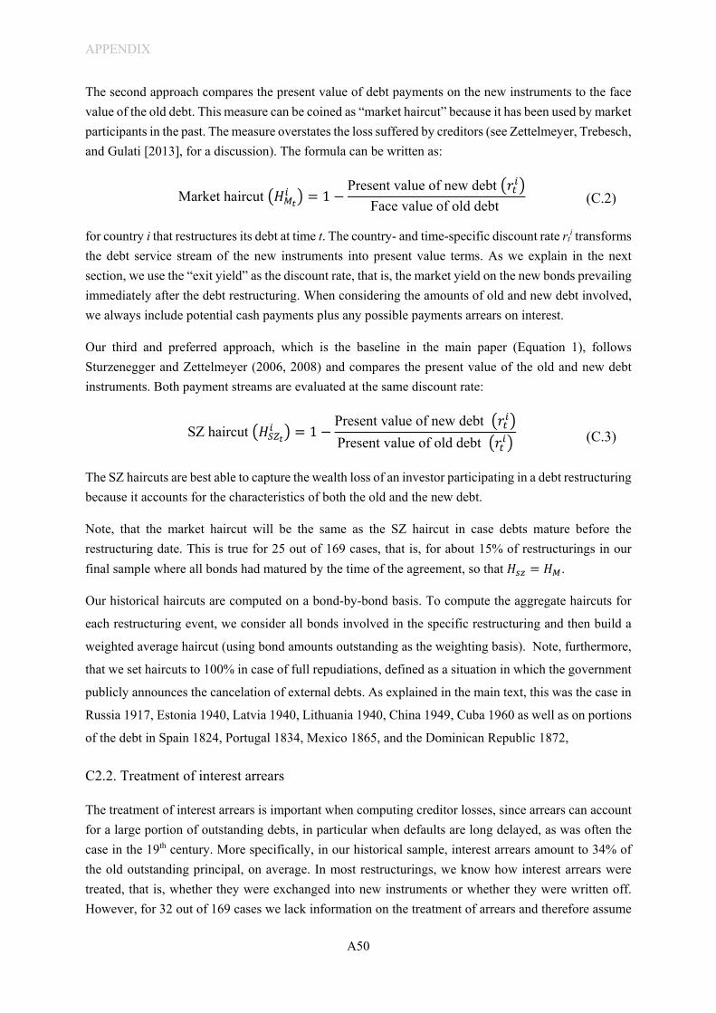
APPENDIX
A50
The second approach compares the present value of debt payments on the new instruments to the face value of the old debt. This measure can be coined as “market haircut” because it has been used by market participants in the past. The measure overstates the loss suffered by creditors (see Zettelmeyer, Trebesch, and Gulati [2013], for a discussion). The formula can be written as:
Market haircut �𝐻𝐻𝑀𝑀𝑡𝑡𝑖𝑖 � = 1 −
Present value of new debt �𝑟𝑟𝑡𝑡𝑖𝑖�Face value of old debt
(C.2)
for country i that restructures its debt at time t. The country- and time-specific discount rate rti transforms
the debt service stream of the new instruments into present value terms. As we explain in the next section, we use the “exit yield” as the discount rate, that is, the market yield on the new bonds prevailing immediately after the debt restructuring. When considering the amounts of old and new debt involved, we always include potential cash payments plus any possible payments arrears on interest.
Our third and preferred approach, which is the baseline in the main paper (Equation 1), follows Sturzenegger and Zettelmeyer (2006, 2008) and compares the present value of the old and new debt instruments. Both payment streams are evaluated at the same discount rate:
SZ haircut �𝐻𝐻𝑈𝑈𝑆𝑆𝑡𝑡𝑖𝑖 � = 1 −
Present value of new debt �𝑟𝑟𝑡𝑡𝑖𝑖�Present value of old debt �𝑟𝑟𝑡𝑡𝑖𝑖�
(C.3)
The SZ haircuts are best able to capture the wealth loss of an investor participating in a debt restructuring because it accounts for the characteristics of both the old and the new debt.
Note, that the market haircut will be the same as the SZ haircut in case debts mature before the restructuring date. This is true for 25 out of 169 cases, that is, for about 15% of restructurings in our final sample where all bonds had matured by the time of the agreement, so that 𝐻𝐻𝑠𝑠𝑠𝑠 = 𝐻𝐻𝑀𝑀.
Our historical haircuts are computed on a bond-by-bond basis. To compute the aggregate haircuts for
each restructuring event, we consider all bonds involved in the specific restructuring and then build a
weighted average haircut (using bond amounts outstanding as the weighting basis). Note, furthermore,
that we set haircuts to 100% in case of full repudiations, defined as a situation in which the government
publicly announces the cancelation of external debts. As explained in the main text, this was the case in
Russia 1917, Estonia 1940, Latvia 1940, Lithuania 1940, China 1949, Cuba 1960 as well as on portions
of the debt in Spain 1824, Portugal 1834, Mexico 1865, and the Dominican Republic 1872,
C2.2. Treatment of interest arrears
The treatment of interest arrears is important when computing creditor losses, since arrears can account for a large portion of outstanding debts, in particular when defaults are long delayed, as was often the case in the 19th century. More specifically, in our historical sample, interest arrears amount to 34% of the old outstanding principal, on average. In most restructurings, we know how interest arrears were treated, that is, whether they were exchanged into new instruments or whether they were written off. However, for 32 out of 169 cases we lack information on the treatment of arrears and therefore assume

APPENDIX
A51
that they were canceled, as was most often the case for those restructurings for which we do have full information.
Regarding amounts, we know the exact size of interest arrears in 39 out of 169 restructurings. For all other cases, we impute the stock of arrears in the restructuring year following standard practice in restructurings of the time and using the information on coupons and principal amounts available to us. More specifically, we add the amounts of interest payments on the outstanding (unpaid) principal for each year from default until agreement, even if the bonds have already matured. To give an extreme example, take the restructuring of Honduras in 1925, which had been in default for 52 years prior to the agreement in 1873. We thus add together all hypothetical interest payments from 1873 until 1925 using the contractual coupon rates of the four bonds affected and including years after maturity (the bonds had matured in 1884, 1885, 1886, and 1904, respectively). Partial interest service during the default period is known and taken into consideration so that we subtract any payments on interest from the imputed arrears amount. Importantly, we do not compound interest, that is, we do not assume interest payments on the arrears, since this was not common practice at the time (none of the 39 restructurings for which we have full information apply compounded interest).
C2.3. Discounting approach
To compute present values, we follow Sturzenegger and Zettelmeyer (2006, 2008) and Cruces and Trebesch (2013) and use the “exit yield” discount rate, which is the secondary market yield of the new instruments that start trading after the restructuring. Whenever possible, we use the secondary market bond price yield of country i at the exit from default. More specifically, for 108 out of 169 historical cases, we use exit yield market data. For another 29 cases, no debt discounting (and thus no yield data) was necessary since the agreements were cash buybacks of already matured bonds. For the remaining 32 debt restructurings, no market yield data was available. Most of these were small, low-income countries with no liquid bonds trading in London and New York. In these cases, we use a “worst yield” approach, which means that we use the highest bond yield observable among non-defaulted sovereigns in the London or New York market at that point in time as a proxy for the country’s own exit yield. The rationale behind this approach is that countries exiting from default usually have rather high yields and this is particularly true for smaller and poorer countries with limited access to external capital markets (that is, those countries who are less likely to have liquid bond prices to start with). The “worst yield” among all debtor countries with liquid bonds that are not currently in default is therefore a useful proxy for the yield of these smaller, poorer countries that just restructured their debt. For example, we use the Argentinian yield of 7.2% in January 1860 for the restructuring of El Salvador in that month, the Chilean yield of 10.4% for the restructuring of Ecuador in March 1955, or the Italian yield of 5.5% for the restructuring of Yugoslavia in July 1895. 9
9 As an alternative approach, we tried using yields of surrogate countries as a proxy in the 46 cases for which actual exit yields were not available (as in Cruces and Trebesch 2013). The idea is to use yields from comparable sovereigns for which price data is available at the restructuring time, such as countries in the same region or of the same size and debt/GDP level. Historically, however, this surrogate approach worked less well, because the number of independent countries is much smaller in history and because most defaults in history were regionally correlated, that is, there is less variation to exploit. Quantitative approaches, such as propensity score matching,

APPENDIX
A52
In order to check the sensitivity of the haircut estimates to the chosen discount rate we also compute haircuts using two alternative discount rates, (i) a risk-free rate (British consols from 1815 to 1918 and US treasury bonds thereafter), and (ii) a 10% flat discount rate across countries and time (the 10% flat rate is regularly used in recent IMF and World Bank reports). Table C3 and Figure C2 illustrate the results for the historical sample.
Table C3: Haircuts in the historical sample: changing the discount rate
Cases Mean Median SD Min Max Market yields (baseline) Market haircut 169 61 63 27 -8 100 SZ-haircut 169 53 52 31 -14 100 10% lump sum rate Market haircut 169 60 61 24 0 100 SZ-haircut 169 51 52 30 -6 100 Lower bound (risk free-rate) Market haircut 169 29 28 43 -89 100 SZ-haircut 169 36 28 37 -87 100
As can be seen, the haircuts using a 10% lump sum rate are rather close to our average baseline estimates using “exit yields”, although the differences by country can be large. The haircut estimates tend to be much lower (about half) when using the risk-free rate. The dispersion of our estimates, however, shows rather similar patterns overall and the number of cases with very high haircuts (close to or at 100%) is also not significantly higher or lower for different discounting approaches.
Figure C2: Haircuts with different discount rates: point estimates by restructuring year
did not show satisfactory results either. We therefore prefer to settle on the plain and simple “worst yield” approach which results in reasonable yield proxies.
-25
0
50
100
Hai
rcut
s in
%
1815 1840 1865 1890 1915 1940 1965 1990
market rate risk free rate 10% rate

APPENDIX
A53
As noted above, the literature on corporate bonds uses bond prices around default events to estimate the size of recovery rates (or haircuts), for example, Moody’s (2011a) or Jankowitsch et al. (2014). To check the relationship between our haircut measure and market prices, Figure C3 plots the estimated haircuts on the vertical axis against the bond prices around 94 default events for which we have reliable pricing data. In line with standard practice, we focus on the post-default prices and use the average bond price one month after the default for each country (portfolio averages). The correlation between the two proxies of investor losses is high, despite the fact that the haircut 𝐻𝐻𝑡𝑡
𝑖𝑖 measures losses at the end of a default spell (in a restructuring), while the prices on the horizontal axis are measured at the start of the default (one month after the credit event). Thus, at the onset of a default, bond markets predict the magnitude of creditor losses in a future restructuring reasonably well.
Figure C3: Haircuts in bond restructurings and bond price at onset of default
C2.4. Historical sovereign bonds: special features and how we deal with them
The historical bonds issued in the pre-WW2 era often share features that are no longer common in today’s bond markets. This section summarizes important historical bond features and explains how we account for them in our haircut calculations.
Sinking funds: Most bonds in history are not due and payable at maturity, but have stretched out amortization schemes, often in the form of so-called “sinking fund” arrangements. The sinking fund goes back to at least the 18th century and its rationale is to smooth out the debtor’s principal redemption schedule and to thereby reduce the risk of default at any given point in time (instead of having repayment spikes at maturity). There are two main types of sinking funds. The first, simpler type is a fixed sinking fund scheme that is comparable to a linear amortization plan - with equal payments stretching from the end of the grace period until maturity. Second, there are cumulative sinking fund schemes. These follow a predetermined, non-linear (typically increasing) annuity amortization plan written in the bond contract. The sinking fund payments were usually forwarded to a fiscal agent predetermined in the bond contract and this agent used the debt service to amortize the bonds. Often, principal amortization payments were
ARG
ARG
ARGAUT
BLZBOL
BOL
BRABRA
BRA
BRA
BGR
BGR
CHL
CHL
CHL
CHN
CHN
CHN
CHN
CHN
CHN
COL
COLCOL
COL
COL
COL
CRICRI
CRICRI
CRI
CRI
CRI
CRICRI
CIV
CIV
CIV
CUB
CUB
CZK
DOM
DOM
DOM
ECU
ECU
ECU
ECU
ECU
EGY
EGY
EGY
SLV
SLV
SLV
SLV
SLV
EST
FIN
DEUDEUDEUDEU
GRC
GRC
GRC
GTM
GTMGTM GTM
HND
HUN
HUN
HUN
ITAJPN
MEX
MEX
MEX
MEX
MEX
MEX
MEX
MEX
NIC
NIC
NICPAN
PRY
PRY
PRY
PER
PERPER
PER
POL
POL
PRT
PRT
PRT
PRT
PRT ROURUS
RUS
RUSRUSRUSRUS
ESP
ESP
ESP
TUR
TUR
TUR
TUR
UKR
URY
URY
URY
URY
VEN
VEN
VEN
VEN
SRB
ZWE
slope:-0.60t-statistic:-5.63
0
20
40
60
80
100
Hai
rcut
size
in %
0 20 40 60 80 100Bond price (1 month after default, average)

APPENDIX
A54
determined by a lottery. In that case, in each period, the fiscal agent randomly selects a subset of bonds (among all outstanding bonds), that will be fully or partially repaid. The lottery is repeated until the sinking fund payments made by the sovereign in that period are depleted. For our calculations, we compute the amortization scheme of each bond and take into account the total sum of repayments at each point, irrespective of whether payments were made to all bondholders or to only a subset of bondholders who won the lottery. This is because the lottery outcomes are random, so one can expect the price effect of the lottery to average out across outstanding bonds.
Bond buybacks: About 50% of the bonds in the sample of historical debt restructurings contain repurchase clauses. These allowed debtor countries to repurchase parts of their bonds in the secondary market. Specifically, debtor countries could use the amounts of the contractually agreed debt servicing (sinking fund) payments for the purchase of bonds (at below-par market prices) instead of repaying the debts at par. Such bond buybacks were reportedly rather common to make partial payments in default situations when bonds typically trade at depressed prices. Unfortunately, numbers are hard to find, since neither the governments nor the fiscal agents are required to report on secondary market buyback operations and the relevant (re-) purchase prices (FBPC 1938, p. 315). As a result, we do not adjust our haircut estimates for these undercover buybacks and instead assume that all debts are redeemed at par. At the same time, we do take into account explicit buybacks where creditors agree to sell outstanding bonds at a fixed price against cash as part of a crisis resolution effort, as was the case in 38 historical restructurings. This approach to deal with buybacks historically is consistent with Cruces and Trebesch (2013). They include 28 buyback agreements of bonds against cash, but also disregard hidden government buybacks in the secondary market (e.g., during Peru’s default in the mid-1990s).
Gold and currency clauses: About 35% of the restructured bond contracts include gold clauses. These gold clauses are not valued when computing haircuts since they were not legally binding, especially after the abrogation of the gold clause in Britain in 1931 and in the US in 1933. Indeed, we find that gold clauses played almost no role in the restructuring agreements, meaning that bonds with or without gold clauses receive the same treatment (that is, the same haircut) and creditors holding gold clause bonds did not even ask for a better deal according to the archival documents. The only cases in which creditors attempted to enforce gold clauses to achieve better treatment are a series of restructurings of French Franc bonds (Brazil 1946, Japan in 1957 and several Eastern European Countries after WW2). 10 Moreover, about 10% of the bonds in our historical sample contain some kind of currency clause. Currency clauses allow creditors to choose in which of a set of currencies they wish to obtain their principal and interest payments, using fixed or variable exchange rates as fixed in the bond contract. Details on creditor choices are however not available and it is again questionable whether the clauses had legal “teeth” and were credible. For simplicity, we therefore assume bonds to be serviced in their currency of issuances, which is similar to the approach of Lindert and Morton (1989).
10 These were mainly debt buybacks in paper francs. If the agreement explicitly provided a higher buyback rate in lieu of the gold clause, gold values were converted in paper francs by the ratio 1:5, as it was done by the CFB (1946).

APPENDIX
A55
C2.5. Further methodological assumptions
This section sets out further methodological assumptions when computing haircuts.
Timing: The month of the final agreement serves as a baseline date to compute cash flow streams. From there all interest and principal payments are computed on a quarterly or semi-annual basis, depending on the contractual terms and the coupon frequency. In 16 cases we calculated annual cash flow streams due to a lack of data. This simplification is also made in Lindert and Morton (1989) or Cruces and Trebesch (2013). Shifting from yearly to monthly or quarterly cash flows had no or only minimal effects on the final estimated haircut. We assessed this based on 20 exemplary bonds across our sample.
Country break-ups and newly independent countries: Several sovereign defaults occurred just prior to, or as a consequence of, state break-ups. For each country break-up case, we gathered detailed information on how the successor states agreed to apportion the old outstanding debt among each other. We then track the settlements on these apportioned debts and calculate the haircuts in each of the successor states. Prominent break-up cases involving a default include:
- The Central American Federation, which went in default in 1828. The successor states agreed to apportion the debt in 1832 in the aftermath of the break-up. 11
- Gran Colombia, which defaulted in 1826. Debt apportionment was agreed in 1834. 12 - The Ottoman Empire, which defaulted in 1914. The debt allotment among the successor states
was a long and disputed process, which ended only in the late 1920s. 13 - Austria-Hungary, which also defaulted in 1914 and which also saw a long debt resolution
process of the various successor states, which took until the 1960s. 14
11 Costa Rica assumed 1/12 (0.013m£) of the 6% bonds, 2/12 was allotted to El Salvador, Guatemala assumed 5/12 of the defaulted 6% bonds, Honduras assumed 2/12 of the debt, and the remaining 2/12 amounting to £0.0272m was assigned to Nicaragua. The restructuring cases involving old defaulted debts of the Central American Federation are Costa Rica in June 1940, El Salvador Jan. 1860, Guatemala May 1856, Honduras Jan. 1867 and Nicaragua Jan. 1874. 12 Specifically, 50% of old principal (£3.3m) was apportioned to Colombia (formerly New Granada), 21.5% (or £2.1m) was assigned to Ecuador, and 28.5% (£2.8m) to Venezuela. The restructuring cases involving old debts of Gran Colombia include New Granada/Colombia in Jan. 1845, Ecuador in Sept. 1855, and Venezuela in Sept. 1840. 13 The final dissolution of the Ottoman Empire started in the early 20th century. After WW1, the Treaty of Lausanne of 1923, constitutes the first formal agreement to apportion the old Ottoman debt, but several successor states objected to their share, followed by an arbitration process coordinated by the League of Nations. Eventually, 65.4% of the Ottoman debt was apportioned to Turkey and the remainder of 34.6% to the other successor states (with Albania 1.26%, Assyr 0.02%, Bulgaria 1.39%, Greece 8.54%, Serbia-Croatian Slovene States 4.2%, Nedjd and Hedjaz 1.26%, Iraq 5.25%, Italy 0.19%, Syria and Lebanon 8.41%, Palestine 2.54%, Transjordania and Maan 0.67%, Yemen 0.91%). The restructuring cases involving old Ottoman debt include Bulgaria in Oct. 1960, Greece in Dec. 1965, Trans-Jordan and Maan in Jul. 1936, Turkey in June 1928 and 1933, and Serbia-Croatian Slovene States in 1959/1960. Iraq paid off its old Ottoman debt share between 1928 and 1934, Italy in 1932, Palestine in 1928, and Syria and Lebanon before 1933. The defaults of Albania, Assyr, Saudi Arabia (formerly Nedid and Hedjaz), and Yemen remained unresolved, that is, no repayment occurred. 14 After WW1, the debt of Austria-Hungary was apportioned in the Lausanne agreement 1923 and in further supplementary agreements in the 1930s. The final settlement was protracted and got finalized only during the 1950s and 60s. The restructuring cases involving old Austrian-Hungarian debt include Austria in Dec. 1952 and Dec. 1957 (Austria-Hungary old debt share: 11%), Czechoslovakia in Jan. 1964 (share: 20%), Hungary in 1953 and March 1956 (share: 27%), Poland in March 1967 (share: 6%), Romania in Feb. 1965 (share: 22%), and Yugoslavia in Oct. 1960 (share: 14%).

APPENDIX
A56
Selective agreements: We calculate haircuts for each debt restructuring implemented with external foreign creditors. Hence, selective agreements of the same debtor country but different creditor groups were coded separately in the raw dataset. However, as explained above we do merge cases of the same default even in the main paper and analysis. In case an agreement is explicitly targeted (and/or restricted) to a certain creditor nationality, we assume that all targeted bonds of that creditor group are settled by this agreement.
Missing maturity or amortization data: For about 15% of the historical debt instruments, the maturity date is not available, although we do have details on the redemption scheme and amounts involved. Recall that these were not bullet maturity bonds but mostly sinking fund bonds with a very stretched-out repayment schedule, often over a period of 40 years or more. For investors at the time, the maturity date was therefore not a crucial piece of information, also because creditors were unlikely to witness it in their lifetime. In case we lack the maturity date, we assume that the maturity ends at the date of the last amortization payment, as inferred from the contractual terms of the bond. Furthermore, in 38 restructurings we had only partial information on the payment schedule of one or more of the bonds involved, meaning that we lack some or all details on the precise sinking fund scheme. In these cases, we assume a cumulative sinking fund of the amortization schedule (comparable with an annuity scheme) since this was the most common approach in the 19th and early 20th centuries.
Perpetuities and consols: About 3% of the defaulted bonds for which we compute haircuts are perpetuities, meaning that they have no predetermined maturity date. For these instruments, we follow standard practice and approximate the net present value of the cash flow by the face value to coupon ratio. In case the start date of the amortization and sinking fund payments are not explicitly stated, which is rare, we assume that amortization starts immediately, since this is the case for almost all bonds in our historical sample.
Contingent debts: Nine restructurings in our sample involve bonds with contingent payments, meaning that the amounts of future debt service were contractually linked to a specific revenue stream. 15 For example, in the 1898 restructuring in Greece, the bond contracts entail a lower bound of debt service payments of 2.5% per annum. On top of this, the contract stated that 49.2% of the receipts from stamp taxes, tobacco taxes, and monopolies (annual receipts above 28.9m drachmae) were divided equally between interest and amortization payments. Similarly, in the Chilean debt restructuring in 1948 creditors could choose between fixed and variable interest rates. For the variable rate bonds, the annual interest payments were fully contingent and consisted of 50% of profits derived from the Chilean Nitrate and Iodine Sales Corporation as well as income tax paid by copper companies. For these and related cases, we compute a hypothetical debt service stream by collecting data on the actual debt service streams based on the bondholder’s manuals in normal times (pre-default), as well as historical data on the underlying revenue streams (from taxes or monopoly incomes). These imputed contingent debt service payments are then used to compute present values and haircuts for each bond at the point of the restructuring.
15 Namely in Chile 1948, Colombia 1861, Dominican Republic 1934, Ecuador 1895, Greece 1898 and 1964, Mexico 1831 and 1942, and Turkey 1881.

APPENDIX
A57
Interest/coupon payments: Coupon rates are available for all defaulted bonds in our historical sample and these are almost always fixed. We therefore do not need to make strong assumptions when calculating future interest cash flows (except for the 9 bonds with contingent interest payments, see bullet point above). In particular, we do not need to make assumptions on forward interest rates as in the case of floating-rate loans that were dominant in sovereign debt markets of the 1970s or 1980s.
Stripped coupons: We are aware that in the 19th century there are a few reported cases in which investors “stripped” coupon and amortization payments into two separate instruments, so as to sell the stripped coupons on the secondary market at a discount. This was attractive for speculative buyers since sovereigns often continued partial interest payments in default, while halting amortization. However, this was not a dominant trading phenomenon at the time and there is a lack of documentation and data so that we ignore any stripped coupon instruments when computing haircuts.
Holdouts: The haircut computations in this paper aim to capture the loss of the average creditor participating in the restructurings. We therefore do not explicitly compute the losses or gains of holdout creditors, also because the details on side-deals with holdouts are not usually known (see Fang, Schumacher, and Trebesch [2020] for a detailed discussion). More generally, when computing haircuts, we use the amounts actually restructured and disregard debts that were not restructured (and possibly continue to be serviced). Nevertheless, for completeness, we did collect information on holdouts and gathered detailed information for 44 of the deals. In this subsample, the average creditor participation rate was 91%, with a standard variation of 9%, indicating that participation was generally rather high and similar to the average participation rate in sovereign bond restructurings since the late 1990s (see Das, Papaioannou, and Trebesch [2012]).
Previously restructured debt: Previously restructured bonds are treated the same way as other old instruments. The relevant future payment streams can be easily computed given the detailed knowledge of the terms of previous restructurings. In total, we find that of all 693 defaulted bonds in our historical sample, 286 were affected by more than one default and restructuring (about 40% of the sample). Of these, 224 were restructured twice, 32 were restructured three times, 13 were restructured four times, and the remaining 17 bonds were restructured five times or more. These numbers are remarkable and mirror the fact that many governments are serial defaulters in the 19th and early 20th centuries (Reinhart et al. 2003). Moreover, many historical bonds had very long maturities (of up to 40 or 50 years), which makes it more likely that the same bond witnesses several defaults.
The most extreme example is Mexico, which originally issued bonds in 1824/1825 and restructured these a total of 8 times over a period of more than 100 years. Mexico first went into default on the bonds in 1827. In 1831, part of the interest arrears was capitalized into new deferred bonds and the original debt service resumed on all other instruments. In 1833, Mexico defaulted on the just issued deferred bonds and restructured them into consolidated bonds in 1842 (exchange 1). As early as 1851, the consolidated bonds were again exchanged into new 3% bonds, which went into default in 1864 (exchange 2). The accrued interest on these bonds was exchanged into a new 3% bond in early 1864 and the debt service on all other instruments resumed (exchange 3). Just two years later, in 1886, Mexico restructured its entire stock of outstanding bonds, including the previously restructured debt, into new

APPENDIX
A58
3% bonds (exchange 4), which were again restructured into a large 5% bond more than 10 years later, in 1899 (exchange 5). After a renewed default in 1914, another restructuring agreement was concluded in 1922, which further lowered the scheduled interest payments and extended the maturities of the previously restructured bonds (exchange 6). Mexico defaulted again in 1924 and a new debt agreement was signed in 1925 (exchange 7). After a new default in the interwar years, Mexico restructured again in 1942 (exchange 8). The last payment on these bonds was finally made in 1960. In our main sample, each of these 8 restructurings is a separate agreement with its own haircut. As in Cruces and Trebesch (2013) or Reinhart and Trebesch (2016) it is possible to compute “cumulative haircuts” if two or more agreements occur in the same default spell.
Administrative fees: Bondholder associations such as the CFB typically charge a small percentage fee to cover their expenses of renegotiating the debt with sovereigns. We could collect detailed information on fees in 35 out of the 169 restructuring cases in our historical sample. The data show that the administrative charges vary between 0.5% and 1.5% of principal restructured. For all other cases, we do not have exact details on the fees. We therefore disregard any fees paid by creditors. This is consistent with the approach in Cruces and Trebesch (2013).
Exchange rate conversions: Our dataset on defaulted bonds focuses on hard currency debt, meaning bonds issued in British Pounds and US dollars. However, some of the restructurings also include bonds issued in French Francs and other currencies. 16 More precisely, 20% of deals in our sample feature bonds of different currencies. To obtain the overall haircut in these cases, we convert all amounts into US dollars using the exchange rates provided by Reinhart and Rogoff (2009) and Officer (2018, https://www.measuringworth.com/).
16 In our historical sample, 56% of bonds are denominated in British pound, 17% in US dollars and 10% in French franc. Another 11% of bonds are denominated in various other foreign currencies, including the Swiss Franc, Swedish kronor, Dutch Florin, Italian Lire, Belgian Franc, German Mark, Japan Yen, Czechoslovakian Kronor, and Spanish Pesetas. The remainder (6% of bonds) are denominated in domestic currencies, namely those pseudo-domestic bonds that were predominantly sold to foreign bondholders and typically traded in London or New York (see the discussion on case selection criteria and pseudo-domestic restructurings above).
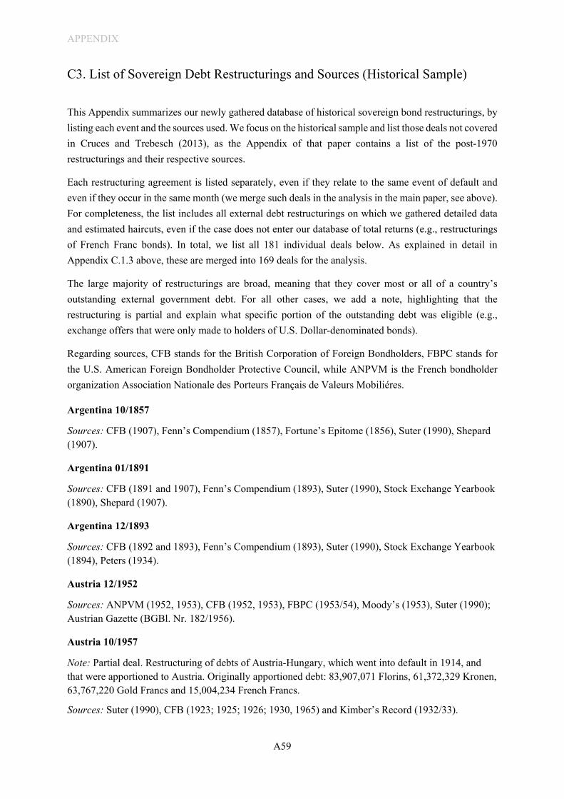
APPENDIX
A59
C3. List of Sovereign Debt Restructurings and Sources (Historical Sample)
This Appendix summarizes our newly gathered database of historical sovereign bond restructurings, by listing each event and the sources used. We focus on the historical sample and list those deals not covered in Cruces and Trebesch (2013), as the Appendix of that paper contains a list of the post-1970 restructurings and their respective sources.
Each restructuring agreement is listed separately, even if they relate to the same event of default and even if they occur in the same month (we merge such deals in the analysis in the main paper, see above). For completeness, the list includes all external debt restructurings on which we gathered detailed data and estimated haircuts, even if the case does not enter our database of total returns (e.g., restructurings of French Franc bonds). In total, we list all 181 individual deals below. As explained in detail in Appendix C.1.3 above, these are merged into 169 deals for the analysis.
The large majority of restructurings are broad, meaning that they cover most or all of a country’s outstanding external government debt. For all other cases, we add a note, highlighting that the restructuring is partial and explain what specific portion of the outstanding debt was eligible (e.g., exchange offers that were only made to holders of U.S. Dollar-denominated bonds).
Regarding sources, CFB stands for the British Corporation of Foreign Bondholders, FBPC stands for the U.S. American Foreign Bondholder Protective Council, while ANPVM is the French bondholder organization Association Nationale des Porteurs Franҫais de Valeurs Mobiliéres.
Argentina 10/1857
Sources: CFB (1907), Fenn’s Compendium (1857), Fortune’s Epitome (1856), Suter (1990), Shepard (1907).
Argentina 01/1891
Sources: CFB (1891 and 1907), Fenn’s Compendium (1893), Suter (1990), Stock Exchange Yearbook (1890), Shepard (1907).
Argentina 12/1893
Sources: CFB (1892 and 1893), Fenn’s Compendium (1893), Suter (1990), Stock Exchange Yearbook (1894), Peters (1934).
Austria 12/1952
Sources: ANPVM (1952, 1953), CFB (1952, 1953), FBPC (1953/54), Moody’s (1953), Suter (1990); Austrian Gazette (BGBl. Nr. 182/1956).
Austria 10/1957
Note: Partial deal. Restructuring of debts of Austria-Hungary, which went into default in 1914, and that were apportioned to Austria. Originally apportioned debt: 83,907,071 Florins, 61,372,329 Kronen, 63,767,220 Gold Francs and 15,004,234 French Francs.
Sources: Suter (1990), CFB (1923; 1925; 1926; 1930, 1965) and Kimber’s Record (1932/33).

APPENDIX
A60
Bolivia 03/1880
Sources: CFB (1879), Fenn’s Compendium (1876), Stock Exchange Yearbook (1880), Suter (1990).
Bolivia 06/1957
Sources: FBPC (1953/54 and 1965/67), Suter (1990).
Brazil 01/1851
Sources: Fenn (1883), Kimber’s Record (1922), Suter (1990), Stock Exchange Yearbook (1900).
Brazil 07/1898
Sources: Fenn’s Compendium (1883), Kimber’s Record (1922), Suter (1990), Stock Exchange Yearbook (1900).
Brazil 10/1914
Sources: Kimber’s Record (1922), Moody's (1919), Suter (1990).
Brazil 11/1943
Sources: CFB (1931, 1933, 1943, 1960), FBPC (1938, 1953/54), Kimber’s Record (1932/33), Moody’s (1931, 1933, 1937, 1943), Suter (1990).
Brazil 03/1946
Note: Partial deal. Franco-Brazil Financial Agreement, relevant for bonds held by French investors.
Sources: ANPVM (1945), CFB (1931, 1933, 1946, 1960), FBPC (1938, 1953/54), Kimber’s Record (1932/33), Moody’s (1931, 1933, 1937, 1946), Suter (1990).
Bulgaria 12/1926
Sources: CFB (1930, 1926, and 1925), Kimber’s Record (1932/33), Moody’s (1926), Suter (1990).
Bulgaria 11/1954
Note: Partial deal. Restructuring of Bulgarian external bonds held by Swiss nationals.
Sources: CFB (1954), FBPC (1955-57), Schweizer Bundesblatt Nr. 7 (17. February 1955).
Bulgaria 03/1959
Note: Partial deal. Restructuring of Bulgarian external bonds held by French nationals.
Sources: CFB (1959), FBPC (1962/64), Suter (1990).
Bulgaria 11/1979
Sources: CFB (1978, 1979).
Note: Partial deal. Restructuring of Bulgarian external bonds denominated in U.S. Dollar.
Bulgaria 10/1987
Sources: CFB (1987). Note: Partial deal. Restructuring of Bulgarian external bonds denominated in British Pound.

APPENDIX
A61
Chile 01/1842
Sources: Fenn’s Compendium (1869), Fortune’s Epitome (1850), Suter (1990).
Chile 06/1884
Sources: Stock Exchange Yearbook (1879-1884), Suter (1990).
Chile 01/1935
Sources: CFB (1935, 1948), FBPC (1935, 1936, 1938, 1937, 1946/49, 1950, 1955/1957), Kimber’s Record (1934).
Chile 03/1948
Sources: CFB (1935, 1948), FBPC (1935-1938, 1946/49, 1950, 1953/54), Kimber’s Record (1934), Moody’s (1936), Suter (1990), World Bank (1949a).
China 02/1936
Note: Partial deal. Minor restructuring of public railway bonds denominated in British Pound.
Sources: CFB (1936), FBPC (1938), Moody's (1939), Suter (1990).
China 05/1936
Note: Partial deal. Minor restructuring of public railway bonds denominated in British Pound.
Sources: CFB (1936), FBPC (1938), Moody's (1939), Suter (1990).
China 08/1936 (2x)
Note: Partial deals. Two separate, small restructuring of public railway bonds denominated in different currencies (British Pound, Guilders, Belgian Franc, French Franc). Implemented on the 6th and 26th of August 1936, respectively.
Sources: CFB (1936), FBPC (1938), Moody's (1939), Suter (1990).
China 10/1936
Note: Partial deal. Minor restructuring of Chinese government bonds denominated in British Pound (Marconi and Vickers’ debt).
Sources: CFB (1936), FBPC (1938), Moody's (1939), Suter (1990).
China 04/1937
Note: Partial deal. Minor restructuring of public railway bonds denominated in British Pound.
Sources: CFB (1936), FBPC (1936), Moody's (1939), Suter (1990).
China 04/1937
Note: Partial deal. Minor restructuring of Chinese government bonds denominated in U.S. Dollar (so-called “Chicago Bank” debts).
Sources: CFB (1936), FBPC (1936).

APPENDIX
A62
Colombia 01/1845
Note: Partial deal. Settlement of the apportioned debt of Gran Colombia.
Sources: CFB (1907), Fenn’s Compendium (1855), Fortune’s Epitome (1856), Suter (1990), Wyllie (1903).
Colombia 10/1861
Sources: CFB (1907), Fenn’s Compendium (1869, 1883), Suter (1875), Wyllie (1903).
Colombia 12/1872
Sources: CFB (1873, 1907), Fenn’s Compendium (1883), Stock Exchange Yearbook (1875), Suter (1875), Wyllie (1903).
Colombia 12/1896
Sources: CFB (1896, 1910), Stock Exchange Yearbook (1898), Suter (1990).
Colombia 04/1905
Sources: CFB (1905/1906, 1907), Stock Exchange Yearbook (1906), Suter (1990).
Colombia 06/1941
Sources: CFB (1941), FBPC (1945), Moody’s (1942), Suter (1990).
Colombia 07/1943
Sources: CFB (1943, 1944), FBPC (1946/49).
Costa Rica 07/1840
Note: Partial deal. Settlement of £0.013m of bonds of the dissolved Central American Federation that had been assigned to Costa Rica.
Sources: CFB (1896, 1907), Suter (1990).
Costa Rica 06/1885
Sources: CFB (1885, 1886), Fenn’s Compendium (1883), Stock Exchange Yearbook (1885), Suter (1990).
Costa Rica 04/1897
Sources: CFB (1896, 1897), Stock Exchange Yearbook (1898), Suter (1990).
Costa Rica 12/1910
Sources: CFB (1910, 1911), Kimber’s Record (1922), Stock Exchange Yearbook (1911), Suter (1990).
Costa Rica 07/1933
Sources: CFB (1932), Moody’s (1935), Kimber’s Record (1934).

APPENDIX
A63
Costa Rica 07/1935
Sources: FBPC (1935, 1938), CFB (1935), Moody’s (1935).
Costa Rica 07/1937
Sources: Moody’s (1939).
Costa Rica 11/1952
Note: Partial deal. Agreement with the U.S. American Foreign Bondholder Protective Council on bonds denominated in U.S. Dollar were restructured into a single new bond.
Sources: CFB (1955), FBPC (1938, 1953/54), Kimber’s Record (1934), Suter (1990).
Costa Rica 10/1955
Note: Partial deal. Agreement with the British Corporation of Foreign Bondholders on bonds denominated in British Pound.
Sources: CFB (1955, 1960, 1965), FBPC (1953/54), Kimber’s Record (1934), Suter (1990).
Costa Rica 10/1965
Note: Partial deal. Restructuring of Gold Franc bond issue of 1911.
Sources: CFB (1965), Kimber’s Record (1934).
Cuba 02/1938
Note: Partial deal. Restructuring of a U.S. Dollar denominated bond (“Public Works” issue).
Sources: FBPC (1938), Moody’s (1938), Suter (1990).
Czechoslovakia 09/1946
Sources: CFB (1946), FBPC (1946/49), Suter (1990).
Czechoslovakia 04/1960
Note: Partial deal. Buyback offer on government bonds denominated in British Pound.
Sources: CFB (1960 and 1965), FBPC (1953/54), Suter (1990).
Czechoslovakia 01/1964
Note: Partial deal. Restructuring of debts of Austria-Hungary, which went into default originally in 1914, and that were apportioned to Czechoslovakia. Originally apportioned debt: 72,603,356 Florins, 26,490,460 Kronen, 380,025,770 Gold Francs and 61,692,765 French Francs.
Sources: Suter (1990), CFB (1923: 79-83; 1925:80-92; 1926:76-92; 1930:93-106 and 1965: 89-113) and Kimber’s Record (1932/33:107).
Czechoslovakia 12/1986
Note: Partial deal. Buyback offer on government bonds denominated in U.S. Dollar.
Sources: CFB (1987).

APPENDIX
A64
Dominican Republic (Santo Domingo) 1872
Note: This is one of the repudiation cases we detected. Unlike the Russian default 1917 and Chinese default 1939, Dominican Republic settled this debt in August 1888.
Sources: CFB (1888, 1889), Fenn’s Compendium (1883), Stock Exchange Yearbook (1890), Suter (1990).
Dominican Republic (Santo Domingo) 11/1893
Sources: CFB (1893, 1894, 1907), Stock Exchange Yearbook (1895), Suter (1990).
Dominican Republic (Santo Domingo) 11/1897
Sources: CFB (1897, 1898), Suter (1990).
Dominican Republic (Santo Domingo) 09/1908
Sources: CFB (1901, 1908), Suter (1990).
Dominican Republic 08/1934
Sources: CFB (1934), FBPC (1938), Kimber’s Record (1934), Moody’s (1935), Suter (1990).
Ecuador 09/1855
Note: Partial deal. Settlement of the apportioned debt of Gran Colombia (totaling £3m).
Sources: CFB (1907), Fenn’s Compendium (1855), Fortune’ Epitome (1856), Spanish American Bondholder Committee (p. 18), Suter (1990), Wyllie (1903).
Ecuador 07/1892
Sources: CFB (1890, 1892), Fenn’s Compendium (1883), Stock Exchange Yearbook (1894), Suter (1990).
Ecuador 02/1895
Sources: CFB (1894), Suter (1990).
Ecuador 10/1897
Sources: CFB (1897, 1908), Suter (1990).
Ecuador 09/1908
Sources: CFB (1908), Suter (1990), Guayaquil and Quito Railway (1908).
Ecuador 03/1955
Note: Partial deal. Restructuring of bonds denominated in US Dollar and British Pound.
Sources: CFB (1955), FBPC (1953/54 and 1955/57), Suter (1990).
Ecuador 08/1958
Note: Partial deal. Restructuring of bonds denominated in French Franc.
Sources: FBPC (1965-67).

APPENDIX
A65
Egypt 11/1876
Sources: CFB (1876, 1907), Fenn’s Compendium (1876, 1883), Stock Exchange Yearbook (1877), Suter (1990), Mc Coan (1877), Wynne (1951).
Egypt 07/1877
Note: Partial deal. Restructuring of bonds raised by Ismail (the viceroy of Egypt) on his private estates, known as the “Daïra loans”.
Sources: CFB (1879, 1907), Fenn’s Compendium (1883), Stock Exchange Yearbook (1878), Suter, Wynne (1951).
Egypt 07/1880
Sources: CFB (1879, 1907), Fenn’s Compendiums (1883), Suter (1990), Wynne (1951).
El Salvador 01/1860
Note: Partial deal. Restructuring of bonds of the dissolved Central American Federation that were apportioned to El Salvador (principal of £0.050m).
Sources: CFB (1877, 1907), Fenn’s Compendium (1855), Suter (1990).
El Salvador 02/1899
Sources: CFB (1898/99), Stock Exchange Yearbook (1895, 1900), Suter (1990).
El Salvador 09/1923
Sources: CFB (1923, 1930), Kimber’s Record (1934), Suter (1990).
El Salvador 05/1932
Sources: CFB (1932), FBPC (1935), Kimber’s Record (1934), Moody’s (1932).
El Salvador 04/1936
Sources: CFB (1933, 1960), FBPC (1935, 1938), Moody’s (1938), Suter (1990).
El Salvador 06/1946
Sources: CFB (1946, 1960), FBPC (1953/54), Suter (1990).
Estonia 1940
Sources: FBPC (1940, 1946/1947), Moody’s (1941).
Finland 08/1945
Note: Settlement of British Pound debt.
Sources: CFB (1946), FBPC (1946/47), Moody’s (1945).
Germany 07/1938
Note: Partial deal. Agreement between Germany and the United Kingdom covering bonds held by British nationals (Dawes Loan and Young Loan).

APPENDIX
A66
Sources: CFB (1938), FBPC (1938), Moody’s (1938), Suter (1990), Transfer Agreement between Germany and Great Britain and Northern Ireland, signed July 1st, 1938.
Germany 08/1938
Note: Partial deal. Agreement between Germany and France covering bonds held by French nationals (Dawes Loan and Young Loan).
Sources: ANPVM (1938), FBPC (1938), Moody’s (1938).
Germany 02/1953
Note: London Debt Agreement on national, subnational, and public/private corporate debt.
Sources: ANPVM (1951-1953), CFB (1952, 1953), FBPC (1951/52, 1953/54), Suter (1990), Glasemann (2009b and 2009a), German Federal Gazette (BGBl. II, 331; BGBl. 1955 I, 86), World Bank (1949c), Deutsche Bundesbank (1991), Conference on German External Debts. (1952).
Greece 12/1878
Sources: CFB (1878, 1907), Fenn’s Compendium (1883), Suter (1990), Wynne (1951), Agreement with Hellenic Government for conversion of Greek Loans of 1825 and 1825.
Greece 03/1898
Sources: CFB (1897, 1898, 1907), Suter (1990).
Greece 08/1935
Sources: FBPC (1936), Moody’s (1938).
Greece 10/1962
Summary: Restructuring of bonds denominated in U.S. Dollar.
Sources: CFB (1962), FBPC (1938, 1965/67), Suter (1990).
Greece 07/1964
Summary: Restructuring of bonds denominated in British Pound.
Sources: CFB (1962), FBPC (1938, 1965/67), Suter (1990).
Guatemala 05/1856
Note: Partial deal. Restructuring of debts of the dissolved Central American Federation that were apportioned to Guatemala.
Sources: CFB (1907), Fortune’ Epitome (1856), Fenn’s Compendium (1855), Suter (1990).
Guatemala 03/1888
Sources: CFB (1888, 1889), Fenn’s Compendium (1883), Stock Exchange Yearbook (1889), Suter (1990).
Guatemala 07/1895
Sources: CFB (1894, 1895), Stock Exchange Yearbook (1896), Suter (1990).

APPENDIX
A67
Guatemala 11/1898
Sources: CFB (1898, 1899), Stock Exchange Yearbook (1899).
Guatemala 05/1913
Sources: CFB(1913), Kimber’s Record (1918).
Guatemala 08/1936
Note: Partial deal. Restructuring of the so-called “Los Altos” bonds denominated in US Dollar.
Sources: FBPC (1936), Moody’s (1938), Suter (1990).
Guatemala 07/1944
Sources: CFB (1944, 1960), FBPC (1938), Suter (1990).
Honduras 01/1867
Note: Partial deal. Restructuring of bonds of the dissolved Central American Federation that were apportioned to Honduras (principal of £0.050m).
Sources: CFB (1907), Fortune’s Epitome (1856), Fenn’s Compendium (1855), Suter (1990).
Honduras 10/1925
Sources: CFB (1925), FBPC (1935), Moody’s (1926), Suter (1990).
Hungary 06/1937
Sources: ANPVM (1938), CFB (1937), FBPC (1938), Moody’s (1938), Suter (1990).
Hungary 11/1947
Note: Partial deal. Restructuring offer for Hungarian bonds held by French nationals.
Sources: ANPVM (1948), FBPC (1965/67).
Hungary 07/1950
Note: Partial deal. Settlement of Hungarian bonds and other external debt owed to Swiss nationals.
Sources: CFB (1968, 1971), Swiss Government Gazette - Bundesblatt Nr. 7, 17. Febr. 1955 (Abkommen zwischen der schweizerischen Eidgenossenschaft und der Ungarischen Volksrepublik betreffend die Abgeltung der schweizerischen Interessen in Ungarn).
Hungary 10/1968
Note: Partial deal. Restructuring of Hungarian external bonds denominated in British Pounds. Sources: CFB (1968, 1971).
Hungary 06/1975
Note: Partial deal. Restructuring of Hungarian external bonds denominated in U.S. Dollar.
Sources: CFB (1975, 1980), Suter (1990).

APPENDIX
A68
Italy 12/1947
Note: Partial deal. Restructuring of Italian bonds denominated in U.S. Dollar.
Sources: CFB (1948), FBPC (1946/49), Suter (1990).
Italy 07/1948
Note: Partial deal. Minor agreement to restructure railway debt assumed by the Italian government.
Sources: CFB (1947, 1948, 1949), FBPC (1946/49), Suter (1990).
Italy 09/1948
Note: Partial deal. Minor agreement between the Italian and British governments to restructure railway debt of the Italian government.
Sources: CFB (1948 and 1947), FBPC (1946/49)
Japan 09/1952
Note: Partial deal. Restructuring of bonds denominated in British Pound and US Dollars.
Sources: CFB (1952), FBPC (1938, 1953/54), Moody’s (1931), Suter (1990).
Japan 02/1957
Note: Partial deal. Restructuring of bonds denominated in French Franc.
Sources: ANPFVM (1956), CFB (1957, 1961), FBPC (1955/57, 1961/1962), Moody's (1957).
Latvia 1940
Sources: FBPC (1940,1946/1947), Moody's (1940).
Liberia 09/1898
Sources: CFB (1898, 1899, 1907), Fenn’s Compendium (1893), Suter (1990).
Liberia 05/1923
Sources: CFB (1924, 1930), Moody’s (1926), Suter (1990).
Liberia 01/1935
Sources: CFB (1935), (FBPC (1938), Moody's (1935), Suter (1990).
Lithuania 1940
Sources: FBPC (1940,1946/1947), Moody's (1940).
Mexico 04/1831
Sources: CFB (1905/06), Fenn’s Compendium (1837, 1840), Suter (1990), Costeloe (2003), Wynne (1951).
Mexico 02/1842
Sources: Fenn’s Compendium (1855), Fortune’s Epitome (1850), Suter (1990), Costeloe (2003), Wynne (1951).

APPENDIX
A69
Mexico 10/1850
Sources: Fenn’s Compendium (1855), Fortune’s Epitome (1850), Payno (1862), Suter (1990).
Mexico 04/1864
Sources: CFB (1898/99), Fenn’s Compendium (1883), Suter (1990). Costeloe (2003).
Mexico 1865
Sources: CFB (1898/99), Fenn’s Compendium (1883), Suter (1990). Costeloe (2003).
Mexico 06/1886
Sources: CFB (1885, 1886, 1898/99), Suter (1990), Costeloe (2003), Mexican Bondholders’ Committee (1876).
Mexico 07/1899
Sources: CFB (1898/99), Suter (1990).
Mexico 06/1922
Sources: Suter (1990), CFB (1922, 1925), FBPC (1935), Kimber’s Record (1930), Moody’s (1926, 1936).
Mexico 10/1925
Sources: CFB (1925), Moodys (1926), Kimber’s Record (1934).
Mexico 11/1942
Sources: CFB (1942), FBPC (1953/54), Stock Exchange Yearbook (1942), Suter (1990), World Bank (1949b).
Mexico 03/1946
Sources: ANPVM (1945), CFB (1946, 1947), FBPC (1953/54), Suter (1990), World Bank (1949b).
Nicaragua 01/1874
Note: Partial deal. Restructuring of bonds of the dissolved Central American Federation that had been assigned to Nicaragua (principal of £0.03m).
Sources: CFB (1877, 1907, 1930), Suter (1990).
Nicaragua 09/1895
Sources: CFB (1895, 1907), Stock Exchange Yearbook (1896), Suter (1990).
Nicaragua 05/1912
Sources: CFB (1912), Kimber’s Record (1918), Stock Exchange Yearbook (1913), Suter (1990).
Nicaragua 10/1917
Sources: CFB (1918), Kimber’s Record (1918), Stock Exchange Yearbook (1918), Suter (1990).

APPENDIX
A70
Nicaragua 07/1937
Sources: CFB (1937), FBPC (1937), Moody’s (1937), Suter (1990).
Panama 01/1940
Sources: Moody’s (1938, 1940), FBPC (1940), Suter (1990).
Paraguay 12/1885
Sources: Association Belge (1903/04), CFB (1885, 1907, 1930), Fenn’s Compendium (1889, 1893), Stock Exchange Yearbook (1895), Suter (1990).
Paraguay 08/1895
Sources: Association Belge (1903/04), CFB (1895, 1907, 1930), Kimber’s Record (1922), Suter (1990).
Paraguay 09/1924
Sources: CFB (1924, 1925), Stock Exchange Yearbook (1925), Suter (1990).
Paraguay 11/1944
Sources: CFB (1944, 1947, 1960), Suter (1990).
Peru 01/1849
Sources: Fenn’s Compendium (1855, 1869), Fortune’s Epitome (1850), Suter (1990).
Peru 05/1889
Sources: Fenn’s Compendium (1889, 1893), Kimber’s Record (1922), Stock Exchange Yearbook (1895), Suter (1990).
Peru 11/1938
Sources: CFB (1938, 1960), FBPC (1937, 1938), Moody’s (1939).
Peru 02/1947
Sources: CFB (1947), FBPC (1946, 1959).
Peru 11/1951
Note: Partial deal. Restructuring of Peruvian external bonds held by American investors.
Sources: CFB (1951), FBPC (1953/54), Suter (1990).
Peru 12/1953
Note: Partial deal. Restructuring of Peruvian external bonds held by British investors.
Sources: CFB (1937, 1947, 1960), FBPC (1953/54), Suter (1990).
Poland 05/1937
Note: Partial deal. Restructuring offer to holders of U.S. dollar bonds.

APPENDIX
A71
Source: CFB (1937), Moody's (1937), FBPC (1937), Suter (1990).
Poland 12/1937
Note: Partial deal. Restructuring of the British Pound tranche of the Polish stabilization bond of 1927.
Sources: CFB (1937, 1938), FBPC (1938), Moody's (1939).
Poland 09/1938
Note: Partial deal. Restructuring of the U.S. Dollar tranche of the Polish stabilization bond issued in 1927. Concluded on Sept 15th.
Sources: CFB (1938), FBPC (1938), Moody's (1939).
Poland 09/1938
Note: Partial deal. Restructuring of U.S. Dollar gold bond of 1920. Concluded on Sept 30th.
Sources: CFB (1938), Moody's (1939), FBPC (1938).
Poland 12/1938
Note: Partial deal. Restructuring offer on Polish U.S. Dollar bond debt that had been lent by the Swedish Krueger group (so-called “Swedish Match” loan). Concludes on Dec 7th.
Sources: FBPC (1938), Moody's (1939).
Poland 12/1938
Note: Partial deal. Restructuring offer on selected U.S. Dollar bonds. Concludes on Dec 31st.
Sources: CFB (1938), Moody's (1939), FBPC (1938).
Poland 09/1951
Note: Partial deal. Restructuring offer for Polish bonds issued in France and for French investors holding Polish government bonds.
Sources: ANPFVM (1951), CFB (1951), FBPC (1953/54), Suter (1990).
Poland 11/1954
Note: Partial deal. Renewed restructuring offer on all remaining instruments of the British Pound tranche of the Polish stabilization bond.
Sources: CFB (1954), FBPC (1953/54).
Poland 03/1967
Note: Partial deal. Restructuring of debts of Austria-Hungary, which went into default in 1914, and that were apportioned to Poland. Originally apportioned debt: 66,618,779 Florins and 22,194,662 Kronen.
Sources: Suter (1990), CFB (1923: 79-83; 1925:80-92; 1926:76-92; 1930:93-106 and 1965: 89-113) and Kimber’s Record (1932/33:107).

APPENDIX
A72
Poland 05/1975
Sources: CFB (1973 and 1975), FBPC (1964/67).
Poland 07/1976
Note: Partial deal. Debt restructuring offer on British Pound denominated bonds of the former Free City of Poland. These debts had been assumed by the Polish government. Concluded on July 9th.
Sources: Suter (1990), CFB (1976 and 1966), FBPC (1962/64).
Poland 07/1976
Note: Partial deal. Debt restructuring offer on U.S. Dollar denominated bonds of the former Free City of Poland. These debts had been assumed by the Polish government. Concluded on July 12th.
Sources: Suter (1990), CFB (1976 and 1966), FBPC (1962/64).
Portugal 1834
Sources: CFB (1907), Fenn’s Compendium (1840), Fortune’s Epitome (1839, 1850), Suter (1990), Wynne (1951).
Portugal 11/1840
Sources: CFB (1907), Fenn’s Compendium (1840), Fortune’s Epitome (1839, 1850), Suter (1990), Wynne (1951).
Portugal 04/1845
Sources: CFB (1907), Fenn’s Compendium (1855), Fortune’s Epitome (1850), Suter (1990), Wynne (1951).
Portugal 07/1856
Sources: CFB (1907), Fenn’s Compendium (1857), Fortune’s Epitome (1856), Suter (1990), Wynne (1951).
Portugal 03/1902
Sources: CFB (1883, 1901/02, 1902/03), Kimber’s Record (1922), Stock Exchange Yearbook (1902), Suter (1990), Wynne (1951).
Romania 02/1959
Note: Partial deal. Restructuring of bonds denominated in French Francs and held by French nationals.
Sources: ANPVM (1958, 1959), CFB (1934, 1936, 1959), Suter (1990).
Romania 02/1965
Note: Partial deal. Restructuring of debts of Austria-Hungary, which went into default in 1914, and that were apportioned to Romania. Original apportioned debt: 144,024,845 Florins, 202,006,693 Kronen, 71,941,574 Gold Francs and 869,000 British Pounds.
Sources: Suter (1990), CFB (1923, 1925, 1926, 1930, 1965) and Kimber’s Record (1932/33).

APPENDIX
A73
Romania 06/1975
Note: Partial deal. Restructuring of bonds denominated in U.S. Dollar.
Sources: CBF (1975), FBPC (1938).
Romania 01/1976
Note: Partial deal. Restructuring of bonds denominated in British Pound. Sources: CFB (1975, 1980), Suter (1990).
Russia 1917
Sources: CBF (1975), FBPC (1938).
Spain 1823
Sources: CFB (1907), Fenn’s Compendium (1837, 1863), Fortune’s Epitome (1850), Suter (1990).
Spain 11/1834
Sources: CFB (1907), Fenn’s Compendium (1837, 1863), Fortune’s Epitome (1850), Suter (1990).
Spain 07/1867
Sources: CFB (1877, 1882, 1907), Fenn’s Compendium (1863, 1883), Fortune’s Epitome (1850), Suter (1990).
Spain 05/1882
Sources: CFB (1882), Fenn’s Compendium (1876, 1883), Kimber’s Record (1922), Stock Exchange Yearbook (1876, 1883), Suter (1990).
Thailand (Siam) 02/1947
Sources: CFB (1947), Moody’s (1948).
Turkey (Ottoman Empire) 12/1881
Sources: CFB (1881, 1907), Fenn’s Compendium (1883), Stock Exchange Yearbook (1883), Suter (1990), Circular “Notice sur la conversion Turque 1881”.
Turkey (Ottoman Empire) 09/1903
Sources: CFB (1903/04).
Turkey 04/1928
Note: Partial deal. Restructuring of debts of the Ottoman Empire, in default since 1914, which had been apportioned to Turkey.
Sources: CFB (1928, 1929), Kimber’s Record (1922, 1934), Moody’s (1934), Conseil de la Dette Publique Répartie de l’Ancien Empire Ottoman (1929).
Turkey 04/1933
Note: Partial deal. Old Ottoman bonds were converted into new Turkish bonds at worse terms.

APPENDIX
A74
Sources: CFB (1933, 1934), Moody’s (1934), Stock Exchange Yearbook (1945), Suter (1990), Conseil de la Dette Publique Répartie de l’Ancien Empire Ottoman (1933a, 1933b).
Turkey 04/1944
Sources: CFB (1944, 1946), Moody’s (1943), ANPVM (1944), Stock Exchange Yearbook (1945), Suter (1990), World Bank (1949d) “Turkey's external public debt history”.
Uruguay 07/1878
Sources: CFB (1907, 1930), Fenn’s Compendium (1883), Stock Exchange Yearbook (1879, 1883), Suter (1990).
Uruguay 08/1891
Sources: CFB (1891, 1907), Fenn’s Compendium (1893), Stock Exchange Yearbook (1892), Suter (1990).
Uruguay 09/1937
Note: Partial deal. Restructuring of Uruguayan bonds denominated in U.S. Dollar.
Sources: CFB (1933, 1937), FBPC (1936, 1937), Moody’s (1939).
Uruguay 01/1939
Note: Partial deal. Restructuring of Uruguayan bonds denominated in British Pound.
Sources: CFB (1939), FBPC (1938 and 1946/49), Moody’s (1939), Stock Exchange Yearbook (1940), Suter (1990).
Venezuela 09/1840
Note: Partial deal. Settlement of the defaulted debt of Gran Colombia that was apportioned to Venezuela.
Sources: CFB (1907, 1908), Fenn’s Compendium (1855, 1883), Fortune’s Epitome (1856), Suter (1990), Wyllie (1903).
Venezuela 03/1859
Sources: CFB (1907), Fenn’s Compendium (1863, 1867), Fortune’s Epitome (1851), Suter (1990).
Venezuela 01/1862
Sources: CFB (1907), Fenn’s Compendium (1869), Suter (1990), Money Market Review (Jan. 3, 1863).
Venezuela 02/1881
Sources: CFB (1880, 1907, 1910), Fenn’s Compendium (1869), Stock Exchange Yearbook (1882, 1883), Suter (1990).
Venezuela 06/1893
Sources: CFB (1893), Suter (1990), Stock Exchange Yearbook (1894).

APPENDIX
A75
Venezuela 06/1905
Sources: CFB (1904/05, 1907, 1930), Kimber’s Record (1922), Stock Exchange Yearbook (1906), Suter (1990).
Yugoslavia (Serbia) 07/1895
Sources: Kimber’s Record (1922), Suter (1990), Economiste européen (1895, p77.; 1896).
Yugoslavia 08/1958
Note: Partial deal. Restructuring of bonds held by French nationals, including Serbian and Yugoslav bonds issued in France.
Sources: ANPFVM (1950, 1951, 1955, 1957, 1958, 1961), CFB (1951, 1958), FBPC (1955/57 and 1958/1961), Suter (1990).
Yugoslavia 02/1960
Note: Partial deal. Restructuring (buyback offer) of bonds denominated in British Pound. Concluded February 23.
Sources: CBF (1962), FBPC (1958/1961).
Yugoslavia 02/1960
Note: Partial deal. Restructuring of apportioned debts of Austria-Hungary, which went into default in 1914. Originally apportioned debt: 93,673,970 Florins, 128,261,015 Kronen, 19,125,930 Gold Francs and 869,000 British Pound.
Sources: Suter (1990), CFB (1923, 1925, 1926, 1930, 1965), Kimber’s Record (1932/33).
Yugoslavia 03/1967
Note: Partial deal. Restructuring (buyback) of bonds denominated in U.S. Dollar.
Source: CFB (1959, 1964), FBPC (1965/67, 1958/1961).
Yugoslavia 06/1967
Note: Partial deal. Restructuring of remaining bonds denominated in British Pound.
Sources: Suter (1990), CFB (1959, 1964, 1967), FBPC (1965/67, 1958/1961).
Zimbabwe 09/1980
Sources: CFB (1980), Moody’s (1980, 1981).
References Appendix C (sources used for the sovereign debt restructuring archive)
Agreement with Hellenic Government for conversion of Greek loans of 1824 and 1825. (1878). London: Printed by Wertheimer, Lea & Co., Circus Place, Finsbury Circus.
Association Belge pour le Défense des Détenteurs de Fonds Publics. (various issues). Rapport Annuel.
ANPVM (various issues) Association Nationale des Porteurs Franҫais de Valeurs Mobiliéres. Rapport présenté à l’assemblée générale.

APPENDIX
A76
Austrian Gazette. (1956). Kundmachung des Bundeskanzleramts vom 19. Juli 1956 über die International Konferenz zur Regelung der österreichischen öffentlichen Vorkriegs-Auslandsschulden, BGBl. Nr. 182/1956.
Conference on German External Debts. (1952). Report of the Conference on German External Debts: London, February-August 1952. London : Stat. Off.
Conseil de la Dette Publique Répartie de l’Ancien Empire Ottoman (various issues). Communication aux Porteurs de Fond Ottomans.
Conseil de la Dette Publique Répartie de l’Ancien Empire Ottoman. (1933a). Avis aux Porteurs de Fonds Ottomans – Accord du 22 Avril 1933 avec la Turquie
Conseil de la Dette Publique Répartie de l’Ancien Empire Ottoman (1933b). Communication aux Porteurs de Fond Ottomans, Le 7 Juin, 1933.
CFB (various issues). Corporation of Foreign Bondholders – Annual Report. Corporation of Foreign Bondholders, London.
Corporation of Foreign Bondholders (1880). Debt of Venezuela. Articles of agreement for conversion and settlement. London: Corporation of Foreign Bondholders.
Costeloe, Michael P. (2003). Bonds and Bondholders: British Investors and Mexico's Foreign Debt, 1824-1888. Praeger Publishers.
Das, U., M. Papaioannou and C. Trebesch (2012). Sovereign Debt Restructurings 1950-2010: Literature Survey, Data, and Stylized Facts. IMF Working Paper 12/203.
Deutsche Bundesbank (1991). Abkommen über deutsche Auslandsschulden – Asugabe von Fundierungsschuldverschreibungenverscheibungen, Mitteilung Nr. 9001/01
Economiste européen (1895, 1896).
Fenn’s Compendium (various issues). Fenn's Compendium of the English and foreign funds, debts, and revenues of all nations; banks, railways, mines, and the principal joint stock companies: Forming an epitome of the various objects of investment and speculation negotiable in London. Fenn, M., London
FBPC (various issues) Foreign Bondholders Protective Council – Annual Reports. Foreign Bondholders Protective Council, New York.
Fortune's Epitome (various issues). Fortune's Epitome of the stock and public funds: With a full account of the bank stock and funds of United States of America, and also of all the other foreign funds. London.
German Gazette. (1955). Gesetz betreffend die Vereinbarung zwischen der Bundesrepublik Deutschland und den Vertretern der Gläubiger und Garantiemächte über die Haftung der Bundesrepublik Deutschland für gewisse österreichische Auslandsanleihen, BGBl. 1954 II p. 504-519.
Glasemann, Hans-Georg. 2009a. Die Auslandsanleihen des Deutschen Reichs und Preussens 1924-1930 : Finanzgeschichte und Katalog. Regenstauf: Edition Münzen und Sammeln.
Glasemann, Hans-Georg. 2009b. Die Schuldtitel der Konversionskasse für deutsche Auslandsschulden 1933-1945. Edition Münzen und Sammeln.
Guayaquil and Quito Railway. (1908). Agreement made at Quito on 30th September, 1908, between the executive government of the Republic of Ecuador and the legal representatives of the

APPENDIX
A77
Guayaquil and Quito Railway Company and of the Council of Foreign bondholders and the Committee of Guayaquil and Quito Railway Bondholders.
Kimber’s Record (various issues). Kimber’s Record on Government Debts and other Foreign Securities. New York: A.W. Kimber and Company.
Mc Coan, James C. (1877). Egypt as it is. New York: Henry Holt and Company.
Mexican Bondholders’ Committee. 1876. Report of the General Meeting of Mexican Bondholders, with Report of Committee and appendices.
Money Market Review Jan 03, 1863.
Moody’s (various issues). Moody’s Manual of Investments and Securities Rating Service: Foreign and American Government Securities. Moody’s Investors Service, New York.
Peters, Harold E. (1934). The foreign debt of the Argentine republic. John Hopkins University Studies in Historical and Political Sciences, Extra Volumes, New Series, No. 21
Republic of Guatemala. (1887). Decree No. 394. Relative to the Arrangement of the Public Debt and Regulations for its Execution. 29th August 1887. London: Council of Foreign Bondholders.
Suter, Christian (1990). Schuldenzyklen in der Dritten Welt: Kreditaufnahme, Zahlungskrisen und Schuldenregelungen peripherer Länder im Weltsystem von 1820 bis 1986. Anton Hain, Frankfurt.
Stamm, Hanspeter (1987). Kooperation und Konflikt im Weltfinanzsystem. Eine Analyse multilateraler Umschuldungsaktionen seit 1956.” Master's Thesis Soziologisches Institut der Universität Zürich.
Stock Exchange Yearbooks (1875-1926, 1938-1945). Various Issues. London.
Swiss Gazette. Abkommen zwischen der Schweizerischen Eidgenossenschaft und der Ungarischen Volksrepublik betreffend die Abgeltung der schweizerischen Interessen in Ungarn, abgeschlossen in Budapest am 19. Juli 1950.
Swiss Gazette. 1955. Botschaft des Bundesrates an die Bundesversammlung zum Handels- und Zahlungsabkommen zwischen der Schweizerischen Eidgenossenschaft und der Bulgarischen Volksrepublik sowie zu dem zwischen den beiden Ländern abgeschlossenen Abkommen betreffend die Entschädigung der schweizerischen Interessen. (Vom 8. Februar 1955), BBl. 1955 I/6749, pp. 245-269 Genehmigung des Abkommens zwischen der Schweizerischen Eidgenossenschaft und der Föderativen Volksrepublik Jugoslawien betreffend die Regelung gewisser schweizerischer Finanzforderung (Vom 19.Februar 1960), BBl. 1960 I/7947, pp. 677-698.
World Bank (1949a). External Debt of Chile. International Bank for Reconstruction and Development.
World Bank (1949b). Mexico’s external public debt, economic and financial causes of debt and debt adjustment plans. International Bank for Reconstruction and Development.
World Bank (1949c). Survey of Germany’s bonded external debt. International Bank for Reconstruction and Development.
World Bank (1949d) “Turkey's external public debt history”. International Bank for Reconstruction and Development.
Wyllie (1903). A letter to G.R. Robinson, ESQ. Chairman of the committee of Spanish American bondholders, on the present state and prospect of the Spanish American loans. London: A.H. Baily and Co. Cornhill.