Embed Size (px)
Citation preview
Paris School of Economics
Master Thesis
“Analyse et Politiques Economiques”
Sovereign debt maturity structure and
political default under electoral
uncertainty
Christophe Terrin
Supervisor:
Pr. Daniel Cohen
Reporter:
Pr. Gilles Saint-Paul
August 25, 2014
Sovereign debt maturity structure and political
default under electoral uncertainty
Christophe Terrin⇤
Abstract
We develop a simple model of sovereign default to study the optimal
choice of sovereign debt maturity structure and the risk of political default
in the context of uncertain upcoming elections. This paper argues that
a benevolent government set the maturity structure in order to complete
markets in the absence of state-contingent contracts, while an opportunis-
tic governments strictly favor either short- or long-term debt depending
on its willingness to repay debt. We also prove that a political default may
happen is two cases: when an opportunistic debtor-friendly government
is unexpectedly reelected; when an opportunistic creditor-friendly govern-
ment issues extensive quantities of debt in order to increase its probability
of reelection but eventually loses. An empirical analysis carried out on
55 presidential elections in 16 emerging financially-integrated emerging
countries shows that maturity is significantly a↵ected by the type of the
incumbent government. This matches the predictions of our model and
suggests that the opportunistic nature of policymakers predominates over
their benevolent nature.
Keywords: Default Risk, Sovereign Debt, Political Uncertainty, MaturityStructure.JEL classification codes: F34, F41.
⇤I am grateful to my supervisor, Pr. Daniel Cohen, for extremely valuable guidance. I
also would like to thank Diego Perez for providing me data on sovereign bond issuance and
maturity.
1 Introduction
Many remarkable examples exist of the close link between default risk and po-litical uncertainty surrounding elections in emerging economies. The most ac-cepted explanation for the sharp decline in sovereign bond prices before the2002 Presidential election in Brazil is the widespread perception among thethen lenders that a Lula presidency would put Brazil on a path towards default-ing on its external debt. The case of Korea in 1997 is also a prime example ofhow uncertainty about repayment decisions may rise in pre-election periods: theopposition candidates’ declarations against the implementation of an economicprogram previously agreed between the IMF and the incumbent governmentraised concerns that are believed to have led to a deepening of the crisis.
Several authors assess the non trivial role of political factors as determinantsof financial distress and default. Tomz and Wright (2007) study the relationshipbetween economic output and sovereign default for 169 default episodes. Theyfind that 38 percent of these defaults occured in years when the output level inthe defaulting country was above the trend value and argue that some of thesedefaults were due to political upheavals that brought to power new coalitionsfavoring default for opportunistic or ideological reasons. Block and Valeer (2005)find that spreads on sovereign bonds are positively a↵ected when a right-wingincumbent is expected to be replaced by a left-wing challenger, and conversely.Little has been said however on how the maturity structure of sovereign debtmay be influenced by these political factors.
In the wake of the international financial crises of the 1990s, when a numberof emerging countries were made vulnerable to debt-rollover crises because ofgovernments borrowing extensive quantities of short-term debt (Mexico in 1994,Indonesia, Korea, Malaysia, Thailand, Russia in 1997-98), proper managementof the maturity profile of sovereign debt has been the subject of many theoreticalstudies. Tirole (2003) and Jeanne (2009) insist on the role of short-term debt asa way for creditors to monitor the government and therefore to give incentivesto implement creditor friendly policies, at the cost of leaving the country morevulnerable to bad shocks. Arellano and Ramanarayan (2013) also show thatshort-term debt provides more incentives to repay, while long-term debt providesa hedge against future fluctuations in interest rate spreads.
The objective of this paper is two-fold: firstly, to identify the determinants ofthe maturity structure of sovereign bond issuances in pre-election periods; sec-ondly, to assess under which conditions the uncertainty surrounding an electionbetween opportunistic candidates may trigger a political default.
This paper develops a three-period model of sovereign debt in which anoutgoing government chooses a time-varying maturity structure of debt underthe imminence of elections. Two governments that di↵er in their willingnessto repay debt compete for o�ce. We assume that there is perfect information
1
among all contracting parties on the type of each government and that creditorsare risk-neutral, therefore bond prices exactly compensates investors for theexpected losses from default. In each period, the incumbent government decideswhether to default on previously issued debt and determine how much to borrowor save. A defaulting government loses access to international markets andsu↵ers a reduction in its endowment for both current and future periods.
In addition to their determination by type - creditor friendly or debtorfriendly - governments are assumed to be either benevolent or opportunistic.Under the benevolent specification, the government in o�ce acts as a socialplanner by maximizing the expected present value of future utility flows. Bycontrast, an opportunistic government only consider future periods if it expectsto be in o�ce: the probability of reelection acts as a discount factor on futureutility flows.
In the first setup of our model, we assume that default is exogenous since itproves more convenient to analyze the optimal maturity choices of policymakers.We find that a benevolent government uses long-term debt for hedging motivesbecause it enables a debtor friendly government, if elected, to avoid costly re-financing. When governments are assumed to be opportunistic, these hedgingbenefits are absent, and maturity is determined by the refinancing conditionsthey face if they get reelected. An investor-friendly government will favor short-term debt as it can refinance it at a high price after the election. Long-term debtis strictly preferred by debtor-friendly governments because they don’t want tosu↵er costly refinancing when reelected.
We then depart from the assumption of exogenous default to study the con-ditions under which a political default may happen. Governments di↵er in theirperception of the cost of defaulting. The benevolent framework acts as a bench-mark where default never happens. Our findings prove that an opportunisticdebtor-friendly government that faces a low probability of reelection may find itoptimal to issue extensive quantities of debt that only an investor-friendly gov-ernment can repay. The same is true for an investor-friendly government but itrequires two additional assumptions: the elected government has the opportu-nity to make an indivisible public investment and the probability of election ofthe creditor-friendly government increases if it is the only one who can handlethe investment and repay the debt. Issuing large amounts of debt so that theother candidate will default surely becomes a vote-winner for the conservativepolicymaker, and this strategy is optimal when reelection is unlikely.
The empirical validity of our findings on maturity choices is tested usinga sample of 16 financially integrated emerging countries with a presidentialsystem. Data on issuances and maturity were provided by Perez (2013) while ourmain source for political orientations and election results was the World Bank’sDatabase of Political Institutions (DPI, 2013). Consistent with our framework,the analysis of the data indicates that, in pre-election periods, maturity shortens
2
when the incumbent is right-wing and lengthens when it is left-wing. Resultshowever suggest that electoral expectations (without controlling for the type ofthe incumbent) have no significant impact on maturity. These findings thereforetend to show that the opportunistic nature of policy makers predominates overtheir benevolent nature.
Related Literature
This study relates to the recent literature on the maturity of sovereign debt.In the absence of state-contingent contracts in international credit markets,Buera and Nicolini (2004) find that the choice of the sovereign debt maturitystructure can help supporting the complete markets Ramsey allocation. Arel-lano and Ramanarayanan (2013) also show that in an environment of incompletemarkets, long-term debt provides hedging benefits that short-term does not, asit helps insure against future idiosyncratic shocks. The benevolent frameworkof our model also highlights this role of the maturity structure. Ahead of uncer-tain elections, the presence of both short-term and long-term debt is imperativefor completing the markets. In particular, the use of long-term debt isolates adebtor-friendly government from the need of costly refinancing.
A drawback of long-term debt is that it exposes lenders to a debt dilutionproblem due to the absence of an explicit seniority structure of sovereign debt inmost countries. Bi (2006) proves that when the risk of dilution is high, investorstend to hold short-term debt as it is more likely to mature before it is diluted.Hatchondo et al. (2010) use a calibrated quantitative model to show that ifthe sovereign could eliminate debt dilution, the number of default per 100 yearswould decrease from 3.10 to 0.42. In our paper, income is deterministic andthere is no uncertainty after the election, so the dilution risk is absent from ourmodel.
An other important strand of the literature focuses on the incentive mo-tives that justify the use of short-term debt. Rodrik and Velasco (1999) andJeanne (2009) note that the threat to withdraw liquid capital may provide agovernment with incentives to carry-out revenue-raising reforms. Arellano andRamanarayanan (2013) also comment on the incentive benefits of short-termdebt. In the model presented in this paper, long-term debt is rationed so thatno commitment problem may arise in the short run.
Few authors analyzed the optimal maturity choice of debt under political un-certainty. Miller (1997) shows that political instability and polarization generateinflation uncertainty that causes the term structure to steepen. More recently,Perez (2013) studies a pooling equilibrium that may arise when internationalcreditors are unaware of the government’s willingness to repay. Long-term debtbecomes less attractive for investor-friendly governments because it pools moredefault risk that is not inherent to them. Our model also introduces two typesof government that di↵er in their willingness to repay, but under conditions of
3
perfect information.
This analysis is also closely linked to theoretical works on political defaults.Amador (2003) and Cuadra and Spapriza (2008) study models of sovereigndefault in which governments have di↵erent preferences regarding to the optimalallocation of resources. They find that higher levels of political uncertainty(measured by the frequency of turnovers) significantly increases the risk of asovereign default, which materializes in higher spreads. The intuition is that ifthe incumbent anticipates a change in government, it is more inclined to transferresources from future periods (when it may not be in o�ce to allocate thoseresources) to the present (when decisions are made according to its preferences),which results in higher levels of debt and hence an increase in the risk of default.We also observe an increase in debt issuances when a political turnover is likely.In our model however, governments do not di↵er by their preferences in termsof the optimal allocation of resources but by their willingness to repay debt.
We share this approach with several other authors, notably Hatchondo, Mar-tinez, and Sapriza (2009)1. They extend recent quantitative models (i.e. Aguiarand Gopinath (2006), Arellano (2008)) by assuming that the two types alternatestochastically in power. They show that a political default may happen whenan “patient” government is unexpectedly replaced by an “impatient” govern-ment. The reason is that a high political stability results in a low probability ofelection of a debtor-friendly government, which in turn translates in high pricesof sovereign debt issuances. A conservative government is therefore more intenton issuing large amounts that only he can repay. Our findings depart fromthose of Hatchondo, Martinez and Sapriza (2009) as default in our model mayonly happen when a pollcymaker in o�ce fears that it will not be reelected.By contrast with what is generally done in the literature, we materialize thedivergence in the willingness to pay the debt by a di↵erence in the perception ofthe cost of defaulting and not by the fact that a government may be “patient”(high discount factor) or “impatient” (low discount factor).
The paper proceeds as follows. Section 2 presents the model declined inthree di↵erent setups. In section 3, the empirical validity of our findings onoptimal maturity choices is tested. Section 4 concludes.
1see also Cole, Dow, and English (1995) and Alfaro and Kanczuk (2005)
4
2 The model
2.1 General setup
We assume that the country lives three periods. Period 0 is the present, period1 is the short run, period 2 is the long run. In period 0, the government canissue one-period short-term debt b
10 and two-period long-term debt b
20. The
addition of short- and long-term debt issued in period 0 is denoted b0. At time1, the government can decide to go on the financial market again and issueone-period debt b21. The income stream (y0, y1, y2) is deterministic and verifiesy0 < y1 y2 so that it is always optimal to borrow at t = 0. If the governmentchooses to default, we assume that its revenue falls to ydef and that it losesaccess to international markets for the current and future periods. ydef is setequal or lower than y0 so that defaulting always results in a sanction on income.
We suppose that there are two types of government, R and D. GovernmentR is investor-friendly while government D is not. The incumbent governmentin period 0 is reelected with probability ↵ in period 1. Unless the contrary isspecified, the incumbent government at t = 0 is of type R.
The risk-free rate is normalized to 0 and the two governments share thesame discount rate, �. The price received for the bonds issued in a given periodincorporates a discount that mirrors the probability of a default in the followingperiods.
In the following, we address this model under three di↵erent specifications.Setup 1 considers default as exogenous. Setup 2 endogenies the decision ofdefault. Setup 3 introduces the option of investing at t=1 and discusses thecase when the probability of reelection is semi-endogenous. In each setup, weconsider the case where the policy maker in period 0 is benevolent and acts asa social planner, with preferences given by:
u(c0) + E0[�u(c1) + �
2u(c2)] (1)
u : R+ ! R being a standard utility function, strictly increasing, concaveand satisfying Inada conditions. We also address the case where the governmentis opportunistic and only cares about future welfare when it is reelected. In thiscase, type k = R,D at t = 0 maximizes:
u(c0) + ↵[�u(c1,k) + �
2u(c2,k)] (2)
The optimal decisions taken in period 0 will depend on the type (R or D)and the nature (benevolent or opportunistic) of the incumbent government.
5
The benevolent specification will then serve as a benchmark to the analysiswith opportunistic policymakers.
2.2 Setup 1: Exogenous Default
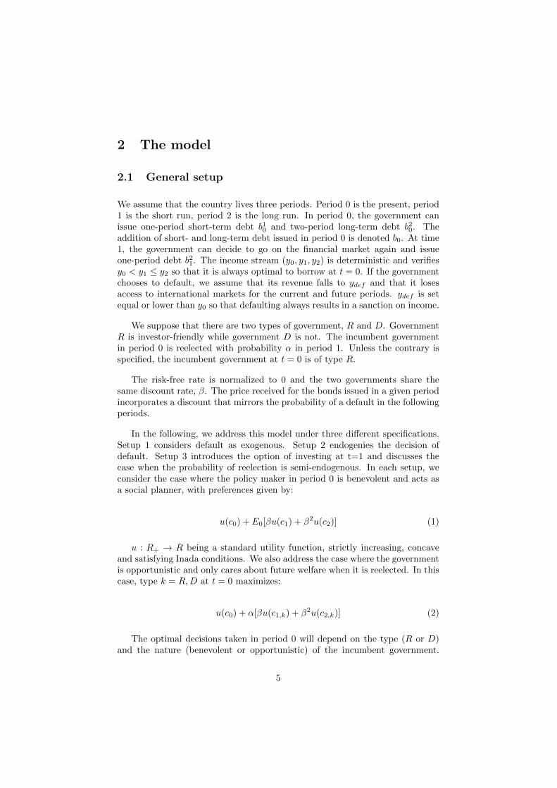
In this setup, it is assumed that type R never defaults while type D defaultswith probability � at each period. To avoid redundancy in the exposition of theproblem, we define �k equal to 0 for k = R and � for k = D. We first solvethe model by assuming that the government at t = 0 cares about future welfareeven if it is not reelected and then consider the problem when it is not the case.
Figure 1: Timeline of events in Setup 1 with R incumbent.
1� ↵
↵Gov. R issues
b10 and b20
R repays b10and issues b21,R
R repays b20and b21,R
D defaults
with proba �
D repays b10and issues b21,D
D defaults
with proba �
D repays b20and b21,D
t = 0 t = 1 t = 2
2.2.1 The benevolent government
When the government at t = 0 cares about future welfare independently ofthe results of the elections, it chooses short- and long-term debt in order tomaximize:
u(c0)+↵
⇥�u(cR1 ) + �
2u(cR2 )
⇤+(1�↵)
⇥�(1� �)u(cD2 ) + �
2(1� �)2u(cD2 )⇤(3)
The problem is solved by backward induction. At t = 2, conditional on nodefaulting at t=0 or t=1, the government consumes c
k2 = y2 � b
20 � b
21,k (for
6

k = R,D). At t = 1, conditional on no defaulting, type k’s problem is:
maxb21,k
u(ck1) + �(1� �k)u(ck2)
s.t. c
k1 = y1 � b
10 + (1� �k)b
21,k,
c
k2 = y2 � b
20 � b
21,k,
c
k2 � ydef .
(4)
The model is calibrated so that the inequality constraint is never bindingfor both governments. Therefore, we focus on interior solutions. The first orderconditions for these two optimization problems write in the same way:
u
0(ck1) = �u
0(ck2) (5)
We now express the government’s problem in period 0 (to simplify notations,we write b
21,k for b21,k(b
10; b
20)) :
maxb10,b
20
u(c0) + �
⇥↵(u(cR1 ) + �u(cR2 )) + (1� ↵)((1� �)u(cD2 ) + �(1� �)2u(cD2 ))
⇤
s.t. c0 = y0 + (↵+ (1� ↵)(1� �))b10 + (↵+ (1� ↵)(1� �)2)b20,
c
k1 = y1 � b
10 + (1� �k)b
21,k,
c
k2 = y2 � b
20 � b
21,k,
c
k1 , c
k2 � ydef .
(6)
Again, our focus is on interior solutions. Using the envelop theorem, thefirst order conditions with respect to b
10 and b
20 are respectively:
(↵+ (1� ↵)(1� �))u0(c0) = �
⇥↵u
0(cR1 ) + (1� ↵)(1� �)u0(cD1 )⇤
(7)
(↵+ (1� ↵)(1� �)2)u0(c0) = �
2⇥↵u
0(cR2 ) + (1� ↵)(1� �)2u0(cD2 )⇤
(8)
We use (5) to simplify equation (8):
(↵+ (1� ↵)(1� �)2)u0(c0) = �
⇥↵u
0(cR1 ) + (1� ↵)(1� �)2u0(cD1 )⇤
(9)
Subtractions (7)�(9) and (9)�(1��)(7) give the same equation for k = R,D:
u
0(c0) = �u
0(ck1) (10)
By issuing short- and long-term debt in period 0, the objective of the benev-olent is twofold. First, as seen in u
0(c0) = �u
0(ck1) = �
2u
0(ck2)2, it transfers
2it is a simple combination of (5) and (10)
7
wealth from period 1 and 2 to period 0 for smoothing purposes. Second, itissues long-term debt so as to equate consumption across non defaulting stateswithin each period: combining (5) and (10) for both values of k, we indeed getc
R1 = c
D1 and c
R2 = c
D2 . To better understand the “hedging benefits” of long-term
debt, consider the alternatives of an incumbent in period 0 whose objective is totransfer income from period 2. It can do so (i) by issuing long-term debt at price↵+(1�↵)(1��)2, or (ii) by issuing short-term debt at price ↵+(1�↵)(1��),expecting that the elected government will refinance it in period 1 at price 1 iftype R is elected, at price (1� �) if type D is elected. It is observed that:
[↵+ (1� ↵)(1� �)](1� �) < ↵+ (1� ↵)(1� �)2 < ↵+ (1� ↵)(1� �) (11)
From the perspective of period 1, the refinancing option is preferred by theelected government R, as b21,R is issued at price 1. By contrast, long-term debtbenefits the elected government when it is of type D, as it can avoid costlyrefinancing. The purpose of long-term debt is to transfer resources from state“R wins the elections” to state “D wins the elections” so that the future levels ofconsumption are unaltered by the outcome of the election. In this sense, issuinglong-term debt is a hedge against the election of a type D.
2.2.2 An example with logarithmic utility
Solving the model with u = log gives the following solutions:
b
10 = y1 � �
W
R
;
b
20 = y2 � �
2W
R
;
b
21,R = b
21,D = 0.
(12)
And the resulting path of consumption is:
c0 =W
R
c
R1 = c
D1 = �
W
R
c
R2 = c
D2 = �
2W
R
where W = y0 + (↵ + (1 � ↵)(1 � �))y1 + (↵ + (1 � ↵)(1 � �)2)y2 andR = 1+(↵+(1�↵)(1��))�+(↵+(1�↵)(1��)2)�2. W can be interpreted as themarket value of the borrower’s income except when it defaults. As commentedearlier, the optimal consumption allocations decline over time at rate � and are
8
constant across states. We denote by m = b20b0
the average maturity at time t=0.
Di↵erentiating b
10,b
20 and m with respect to � and ↵, we find that:
@b
10
@�
> 0;@b
20
@�
> 0;@m
@�
< 0;
@b
10
@↵
< 0;@b
20
@↵
< 0;@m
@↵
> 0.
A increase in the probability of default (due to an increase in � or a decreasein ↵) leads to more issuance of short- and long-term debt. As seen in (12),short-term debt is more sensitive than long-term debt to a change in ↵ or �,therefore the average maturity tends to shorten.
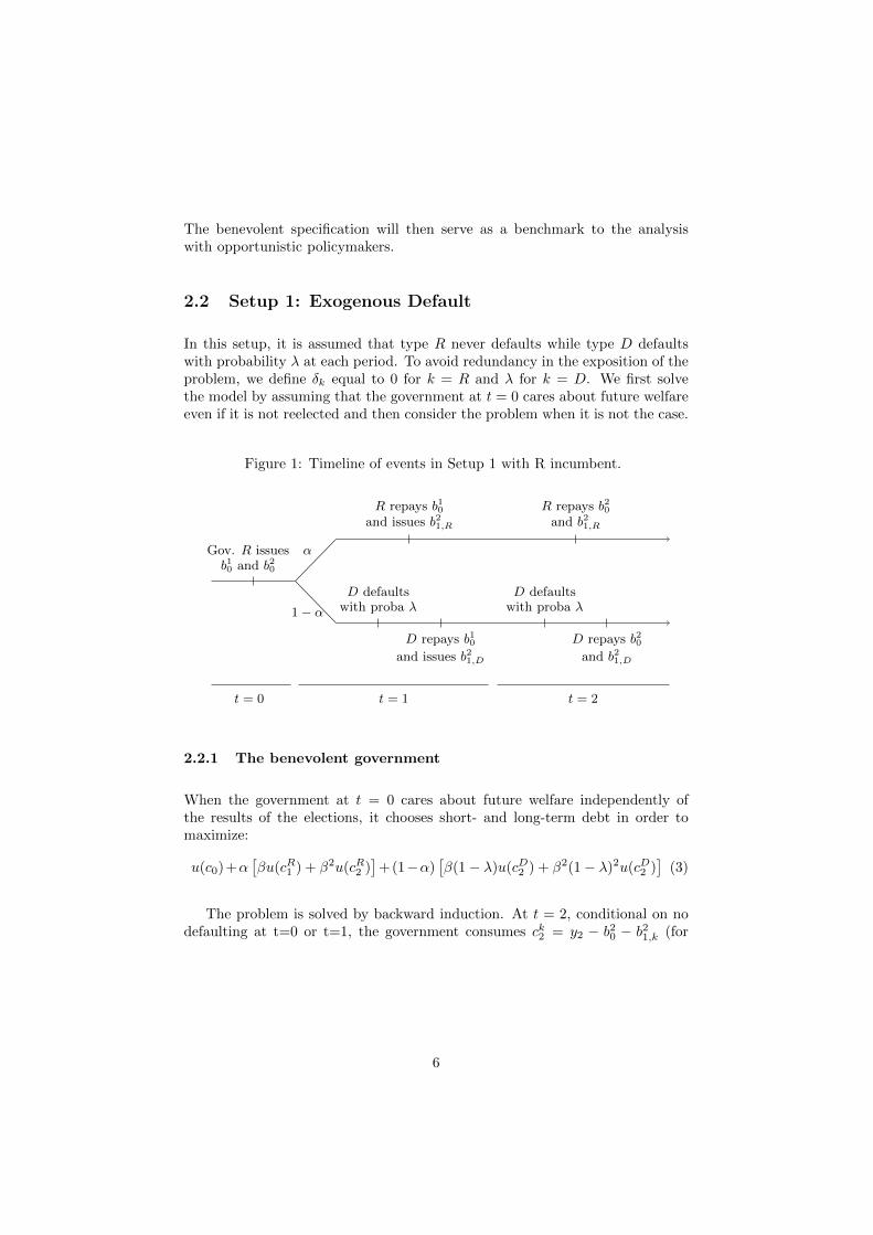
2.2.3 The opportunistic government: type R
Suppose now that the government in period 0 doesn’t care about future welfareif it is not reelected. The government’s problem becomes:
maxb10,b
20
u(c0) + ↵
⇥�u(cR1 ) + �
2u(cR2 )
⇤
s.t. c0 = y0 + (↵+ (1� ↵)(1� �))b10 + (↵+ (1� ↵)(1� �)2)b20,
c
R1 = y1 � b
10 + b
21,R,
c
R2 = y2 � b
20 � b
21,R,
b
10 y1 � ydef + (1� �)(y2 � ydef � b
20),
b
20 y2 � ydef .
(13)
When ↵ = 1, the prices of short- and long-term debt are both equal to 1.Government R is then completely indi↵erent between short- and long-term debt.However, for all values of ↵ lower than 1, the government only issues short-termdebt as it can sell it to a strictly better price than long-term debt. The hedgingbenefits of long-term debt are absent, because the government of type R att = 0 does not care about welfare if it is not reelected. If government R wishesto transfer income from period 2 to 0, it does so by issuing short-term debt thatit refinances if reelected. b20 is then equal to 0 and the first order condition withrespect to b
10 for interior solutions writes:
✓1 + (1� �)
1� ↵
↵
◆u
0(c0) = �u
0(cR1 ) (14)
We derive from this equation that the issuance of short-term debt at t = 0decreases with the probability of reelection. As alpha decreases, the govern-ment gives less weight to future consumption (remember that future utility is
9
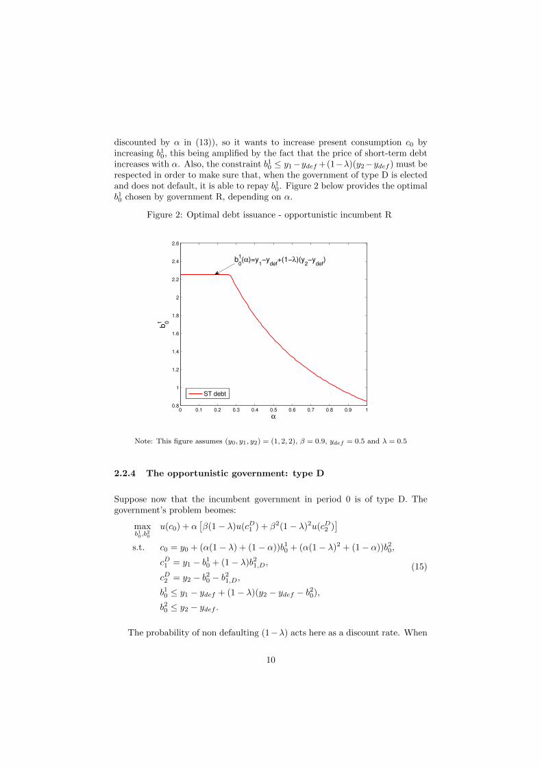
discounted by ↵ in (13)), so it wants to increase present consumption c0 byincreasing b
10, this being amplified by the fact that the price of short-term debt
increases with ↵. Also, the constraint b10 y1�ydef +(1��)(y2�ydef ) must berespected in order to make sure that, when the government of type D is electedand does not default, it is able to repay b
10. Figure 2 below provides the optimal
b
10 chosen by government R, depending on ↵.
Figure 2: Optimal debt issuance - opportunistic incumbent R
0 0.1 0.2 0.3 0.4 0.5 0.6 0.7 0.8 0.9 10.8
1
1.2
1.4
1.6
1.8
2
2.2
2.4
2.6
α
b01
ST debt
b0
1(α)=y1−y
def+(1−λ)(y
2−y
def)
Note: This figure assumes (y0, y1, y2) = (1, 2, 2), � = 0.9, ydef = 0.5 and � = 0.5
2.2.4 The opportunistic government: type D
Suppose now that the incumbent government in period 0 is of type D. Thegovernment’s problem beomes:
maxb10,b
20
u(c0) + ↵
⇥�(1� �)u(cD1 ) + �
2(1� �)2u(cD2 )⇤
s.t. c0 = y0 + (↵(1� �) + (1� ↵))b10 + (↵(1� �)2 + (1� ↵))b20,
c
D1 = y1 � b
10 + (1� �)b21,D,
c
D2 = y2 � b
20 � b
21,D,
b
10 y1 � ydef + (1� �)(y2 � ydef � b
20),
b
20 y2 � ydef .
(15)
The probability of non defaulting (1��) acts here as a discount rate. When
10
↵ = 1, the prices of short- and long-term debt exactly mirror these discountrates: government D is indi↵erent between issuing short- or long-term debt.When ↵ is lower than 1, government D takes advantage of the fact that pricesare positively a↵ected by the eventuality that an investor friendly governmenttakes power. Importantly, long-term debt prices is more sensitive than short-term debt prices to a change in ↵, so the government strictly prefers to issuelong-term debt as long as it is equal or lower than y2 � ydef , the disposableincome of period 23. To better understand this strict preference for long-termdebt, consider again a transfer of income from period 2 to period 0: governmentD can either issue long-term debt at price ↵(1��)2+(1�↵), or issue short-termdebt at price ↵(1� �) + (1�↵) and then refinance it at price 1� � in period 1.Given that ↵(1� �)2 + (1�↵) > (↵(1� �) + (1�↵))(1� �), issuing long-termdebt is strictly preferred to the second option.
2.2.5 Concluding comments
In this set up, we found that the optimal maturity structure of debt issuancesin pre-election periods is highly dependent on the nature of the governmentof the day. In the benevolent framework, maturity is completely and uniquelydetermined by the uncertainty as to the outcome of the elections while the typeof the incumbent is of no importance. By contrast, under the opportunisticassumption, the optimal maturity choice is primarily driven by the type ofthe incumbent, the probability of reelection only accounting for the issuancemagnitude. The empirical analysis presented in the third section of this papertests these two frameworks in order to find whether it is the benevolent oropportunistic nature that predominates in observed choices of maturity.
3In this setup, we abstract from constraints that may arise due to commitment issues by
assuming that b21 has to be non negative. Setup 2 provides insights on this particular problem.
11
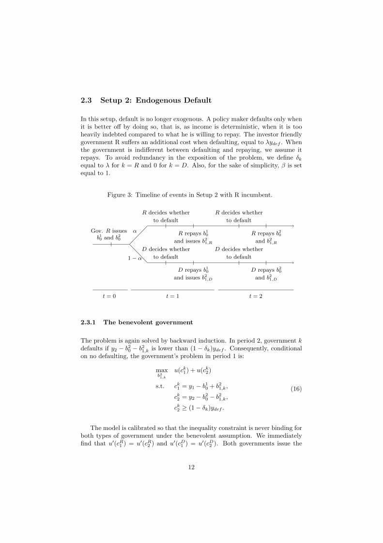
2.3 Setup 2: Endogenous Default
In this setup, default is no longer exogenous. A policy maker defaults only whenit is better o↵ by doing so, that is, as income is deterministic, when it is tooheavily indebted compared to what he is willing to repay. The investor friendlygovernment R su↵ers an additional cost when defaulting, equal to �ydef . Whenthe government is indi↵erent between defaulting and repaying, we assume itrepays. To avoid redundancy in the exposition of the problem, we define �k
equal to � for k = R and 0 for k = D. Also, for the sake of simplicity, � is setequal to 1.
Figure 3: Timeline of events in Setup 2 with R incumbent.
1� ↵
↵Gov. R issues
b10 and b20
R decides whether
to default
R repays b10and issues b21,R
R decides whether
to default
R repays b20and b21,R
D decides whether
to default
D repays b10and issues b21,D
D decides whether
to default
D repays b20and b21,D
t = 0 t = 1 t = 2
2.3.1 The benevolent government
The problem is again solved by backward induction. In period 2, government kdefaults if y2 � b
20 � b
21,k is lower than (1 � �k)ydef . Consequently, conditional
on no defaulting, the government’s problem in period 1 is:
maxb21,k
u(ck1) + u(ck2)
s.t. c
k1 = y1 � b
10 + b
21,k,
c
k2 = y2 � b
20 � b
21,k,
c
k2 � (1� �k)ydef .
(16)
The model is calibrated so that the inequality constraint is never binding forboth types of government under the benevolent assumption. We immediatelyfind that u
0(cR1 ) = u
0(cR2 ) and u
0(cD1 ) = u
0(cD2 ). Both governments issue the
12
same amount: b21,R = b
21,D = (y2�b20)�(y1�b10)
2
In period 0, the benevolent government solves:
maxb10,b
20
u(c0) + u(c1) + u(c2)
s.t. c0 = y0 + b
10 + b
20
c1 = y1 � b
10 + b
21,
c2 = y2 � b
20 � b
21,
b0 y1 + y2 � 2ydef ,
2u((y2 + y1 � b0)/2) � u(y1 � b
10) + u(ydef ).
(17)
The two inequality constraints must be respected for government D not todefault when elected. The first inequality corresponds to type D’s disposableincome in period 1 and 2. The second inequality is derived form
u(y1 � b
10 + b
21) + u(y2 � b
20 � b
21) � u(y1 � b
10) + u(ydef ) (18)
This inequality corresponds to what Arellano and Ramanarayanan (2013)call the incentive constraint, here written for government D. As long as b21 is nonnegative, this constraint is always verified. However, if the elected governmentat t = 1 inherits an amount of long-term debt larger than y2 � ydef and (18) isnot verified, it becomes optimal for the elected government D to set b21 = 0 anddefault in period 2.
Lenders anticipate this problem of commitment by setting a price of ↵ forlong-term debt if (18) is not verified for D, and 0 if it is not verified for Reither4. In this sense, prices are more sensitive to long-term than to short-termdebt. An assumption of our model is that punishment only arises in the eventof an explicit default, so short-term debt provides an incentive for the electedgovernment to repay that long-term debt does not.
A larger ydef a↵ects the problem at t = 0 in two ways. First, it reduces themaximum overall amount of debt that government D is willing to repay in thefuture (constraint b0 y1 + y2 � 2ydef ). Second, for a given b0, it increasesthe minimum amount of short-term debt that must be issued in order for theelected government at t = 0 to be intent to save if needed (incentive constraint).
Assuming that the constraint b0 y1 + y2 � 2ydef is not binding, the firstorder conditions give c0 = c
R1 = c
D1 = c
R2 = c
D2 = (y0 + y1 + y2)/3. As long
4The incentive constraint for government R is u(y1 � b10 + b21) + u(y2 � b20 � b21) � u(y1 �
b10) + u((1� �)ydef ). It is less constraining than the incentive constraint for D, so as long as
the latter verifies, the former does also.
13
as the incentive constraint is verified, the policy maker at t = 0 is indi↵erentbetween issuing short- or long-term debt. Similarly to setup 1, the type of theincumbent government in period 0 has no influence on the problem.
2.3.2 The opportunistic government: type R
Suppose now that the government in period 0 doesn’t care about future welfareif it is not reelected. Government R’s problem becomes:
maxb10,b
20
u(c0) + ↵[u(cR1 ) + u(cR2 )]
s.t. c0 = y0 + b
10 + b
20
c
R1 = y1 � b
10 + b
21,
c
R2 = y2 � b
20 � b
21,
b0 y1 + y2 � 2ydef ,
2u((y2 + y1 � b0)/2) � u(y1 � b
10) + u(ydef ).
(19)
For ↵ = 1, the solution does not change compared to the benevolent frame-work: the first inequality constraint is not binding and the policy maker issuesdebt in order to smooth consumption equally across periods: c0 = c
R1 = c
R2 .
As ↵ decreases however, it gradually increases its issuance of debt in order toconsume more at t = 0 as long as the inequality constraint b0 y1 + y2 � 2ydefdoes not bind. We denote by ↵
0 the probability of reelection for which theinequality becomes binding. This preference for present consumption stemsfrom the first order condition u
0(c0) = ↵u
0(c1) = ↵u
0(c2). Also, as b0 increases,the incentive constraint tightens and the maximum average maturity allowedshortens.
Proposition 1. Suppose the incumbent government in period 0 is of type R.The elected government at t = 1 never defaults.
The proof can be found in Appendix 1. Issuing b0 larger than y1+y2�2ydefcan be thought of as an interesting option when government R expects thatit will not have to face repayment because of a low probability of reelection ↵.Lenders, however, would sanction this tentative by setting a low price ↵ for long-term debt, as they anticipate that only government R would be able to repayin the future. By proposition 1, for all values of ↵ lower than ↵
0, government Rissues b0 = y1 + y2 � 2ydef .
14
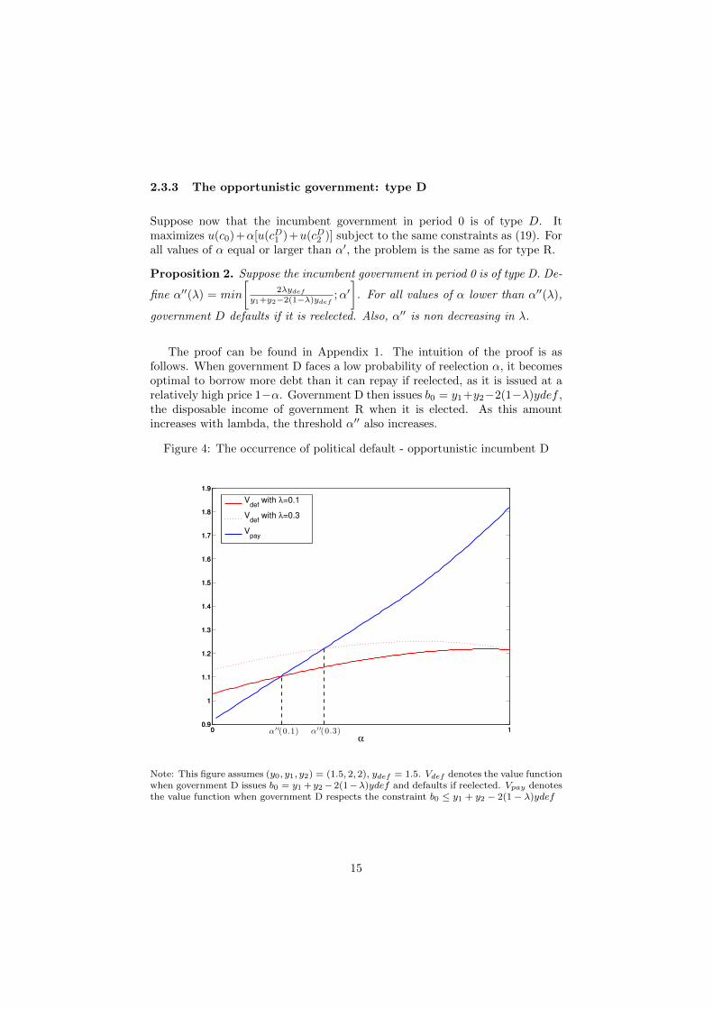
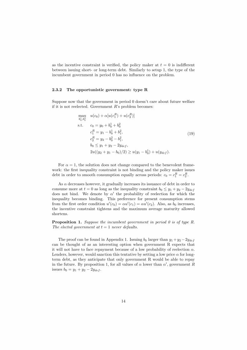
2.3.3 The opportunistic government: type D
Suppose now that the incumbent government in period 0 is of type D. Itmaximizes u(c0)+↵[u(cD1 )+u(cD2 )] subject to the same constraints as (19). Forall values of ↵ equal or larger than ↵
0, the problem is the same as for type R.
Proposition 2. Suppose the incumbent government in period 0 is of type D. De-
fine ↵
00(�) = min
2�ydef
y1+y2�2(1��)ydef;↵0
�. For all values of ↵ lower than ↵
00(�),
government D defaults if it is reelected. Also, ↵00 is non decreasing in �.
The proof can be found in Appendix 1. The intuition of the proof is asfollows. When government D faces a low probability of reelection ↵, it becomesoptimal to borrow more debt than it can repay if reelected, as it is issued at arelatively high price 1�↵. Government D then issues b0 = y1+y2�2(1��)ydef ,the disposable income of government R when it is elected. As this amountincreases with lambda, the threshold ↵
00 also increases.
Figure 4: The occurrence of political default - opportunistic incumbent D
0 10.9
1
1.1
1.2
1.3
1.4
1.5
1.6
1.7
1.8
1.9
α
V
D when λ=0.1
VD when λ=0.3
data3
0 10.9
1
1.1
1.2
1.3
1.4
1.5
1.6
1.7
1.8
1.9
Vdef
with λ=0.1
Vdef
with λ=0.3
Vpay
α′ ′(0.1) α
′ ′(0.3)
Note: This figure assumes (y0, y1, y2) = (1.5, 2, 2), ydef = 1.5. Vdef denotes the value function
when government D issues b0 = y1+y2�2(1��)ydef and defaults if reelected. Vpay denotes
the value function when government D respects the constraint b0 y1 + y2 � 2(1� �)ydef
15
Figure 5: Optimal debt issuance - opportunistic incumbent D
0 1
0.5
1
1.5
α
b0
b0b 0(α) = y1 + y2 − 2(1 − λ )yd ef
b 0(α) = y1 + y2 − 2yd ef
α ′ ′ α ′
Note: This figure assumes (y0, y1, y2) = (1.5, 2, 2), ydef = 0.5 and � = 0.1
2.4 Setup 3: Endogenous Default, Investment and Semi-Endogenous Probability of Reelection
In addition to the previous model, it is now assumed that the elected governmentin period 1 has the opportunity to make an indivisible public investment of sizeK that raises by (1 + ⌧)K the country’s expected output in period 2. Weabstract from maturity issues by assuming that the policy maker at t = 0 canonly issue short-term debt5. Importantly, the decision of investment is madeafter b21 has been issued and K is su�ciently large so that it must be financedby debt. Therefore, if the incumbent government in period 1 prefers to consumeK rather than investing it, it will default in period 2. Lenders anticipate thisproblem by imposing the following constraint in period 1 :
u(y1�b
10+b
21�K)+u(y2�b
21+(1+⌧)K) � u(y1�b
10+b
21)+u((1��k)ydef ) (20)
with �R equal to � and �D equal to 0. The government in period 1 hasto be better o↵ by investing K rather than consuming all b21 and default inperiod 2. If this condition is not verified, international creditors anticipate that
5The possibility to issue long-term debt does not provide further insight compared to what
has already been said in the previous setup.
16
the government will not invest and therefore constrain b
21 to a maximum of
y2 � (1� �k)ydef , or 0 if it is too heavily indebted (b10 > y1 + y2 � 2(1� �k)ydef )
In the opportunistic framework, we discuss the case when the probabilityof reelection is semi endogenous. ↵ is given exogenously, but if government R(government D) in period 0 chooses b10 such that only government R can repayit, invest and avoid default in period 1, then the probability of reelection jumps(drops) to ↵. In the following, utility is assumed to be logarithmic and � is setto 1.
2.4.1 The benevolent government
The elected government’s problem in period 1 is:
maxb21
u(c1) + u(c2)
s.t. c1 = y1 � b
10 �K + b
21,
c2 = y2 + (1 + ⌧)K � b
21,
condition (20) holds.
(21)
The strategy chosen depends on the amount of debt b
10 inherited from the
previous government. We define two thresholds denoted b
1⇤0 (k) and b
1⇤⇤0 (k) such
that:
b
1⇤0 (k) = y1 + y2 + ⌧K � (1� �k)ydef �
q4K(1� �k)ydef + ((1� �k)ydef )2
b
1⇤⇤0 (k) = y1 + y2 + ⌧K � (1� �k)ydef � 2
qK(1� �k)ydef
(22)
The behavior of government k in period 1 depends on the level of pendingdebt b10 compared to these thresholds, as is stated in the following proposition:
Proposition 3. Suppose government k = R,D is elected in period 1.
• When b
10 b
1⇤0 (k), condition (20) is not binding. The government smoothes
consumption equally: c1 = c2.
• When b
1⇤0 (k) < b
10 b
1⇤⇤0 (k), condition (20) is binding. The government
chooses the maximum b
21 such that (21) is verified, and c1 < c2.
• When b
10 > b
1⇤⇤0 (k), the government defaults.
The proof can be found in the appendix. We comment here briefly thethird point. For values of b10 larger than b
1⇤⇤0 (k), there exists no b
21 such that
17
condition (20) holds: the government cannot borrow su�cient funds to investK.Moreover, as b1⇤⇤0 (k) > y1 + y2 � 2ydef , the government is too heavily indebtedand has no choice but to default.
It can also be observed that b
1⇤0 (D) < b
1⇤0 (R) and more importantly that
b
1⇤⇤0 (D) < b
1⇤⇤0 (R). This means that government R can bear a larger amount of
inherited debt than D without defaulting.
For all values of b
10 lower that b
1⇤0 (D), both R and D are unconstrained:
they both smooth consumption equally across periods 1 and 2 by choosing thesame b
21. In the following, it is assumed that the model is calibrated so that
the amount b
10 chosen by the benevolent government in period 0 is lower than
b
1⇤0 (D). The type or the probability of reelection ↵ don’t a↵ect the decision ofthe benevolent policy maker. Debt b10 is issued in order to smooth consumption,and we have:
c0 = c1 = c2 =y0 + y1 + y2 + ⌧K
3(23)
The sum of all incomes and the value created by the investment is equallydivided among the 3 periods.
2.4.2 The opportunistic government: type R
For the moment, the probability of reelection is assumed to be exogenous. Forthe sake of simplicity, � is set so that b
1⇤⇤0 (D) < b
1⇤0 (R)6. Government R’s
problem in period 0 writes:
maxb10,b
21
u(c0) + ↵(u(cR1 ) + u(cR2 ))
s.t. c0 = y0 + b
10,
c
R1 = y1 � b
10 �K + b
21,
c
R2 = y2 + (1 + ⌧)K � b
21,
b
10 b
1⇤⇤0 (D).
(24)
Since b1⇤⇤0 (D) < b
1⇤0 (R), condition (20) for R holds and is not binding as long
as the inequality constraint b
10 b
1⇤⇤0 (D) holds. For ↵ = 1, the problem does
not change compared to the benevolent framework. As ↵ decreases however,government R gradually increases its issuance of debt until it reaches b
1⇤⇤0 (D).
We denote by ↵
⇤⇤ the value for which the inequality b
10 b
1⇤⇤0 (D) becomes
binding.
Proposition 4. Suppose the incumbent government in period 0 is of type Rand the probability of reelection is exogenous. The elected government at t = 1never defaults.
6assuming the contrary complicates the results without providing further insight
18

The proof can be found in appendix 1. This intuition of the proof is thesame to that of proposition 1. For values of ↵ lower than ↵
⇤⇤, government Rsticks to b
10 = b
1⇤⇤0 (D)
Before considering the semi-endogenous probability of reelection assumption,we first describe government R’s problem when it chooses to issue more thanb
1⇤⇤0 (D):
maxb10,b
21
u(c0) + ↵(u(cR1 ) + u(cR2 ))
s.t. c0 = y0 + ↵b
10,
c
R1 = y1 � b
10 �K + b
21,
c
R2 = y2 + (1 + ⌧)K � b
21,
b
1⇤⇤0 (D) < b
10 b
1⇤⇤0 (R),
(25)
The price of b10 naturally drops to ↵ as type D systematically defaults ifelected. Assuming that condition (20) for R is not binding, we find that gov-ernment R issues:
b
10(↵) =
�2y0 + y1 + y2 + ⌧K
1 + 2↵(26)
By doing so, the same amount is consumed at each period when it is elected:(y0 + ↵(y1 + y2 + ⌧K)/(1 + 2↵). The condition b
10 > b
1⇤⇤0 (D) holds as long as:
↵ <
ydef + 2pKydef � 2y0
2b1⇤⇤0 (D)(27)
Note that this condition does not hold when K = 0. The option of invest-ment is necessary for the strategy “R borrows more than what type D is willingto repay” to exist. We also observe that the expression found for the uncon-strained optimal b10 is decreasing with ↵ and that b10(0) = �2y0 + y1 + y2 + ⌧K.When � = 1 (government R is highly averse to default), both b
1⇤0 (R) and b
1⇤⇤0 (R)
are equal to y1+y2+⌧K, therefore, by proposition 3, condition (20) for R alwaysholds and never binds. In this case, the value function, denoted Vdef,�=1(↵),writes:
Vdef,�=1(↵) = (1 + 2↵)u
✓y0 + ↵(y1 + y2 + ⌧K)
1 + 2↵
◆(28)
We also define Vpay, the value function when government R respects theconstraints b10 = b
1⇤⇤0 (D):
Vpay(↵) = u(y0 + b
1⇤⇤0 (D)) + 2↵u
✓y1 + y2 + ⌧K � b
1⇤⇤0 (D)
2
◆(29)
Both Vpay and Vdef are increasing with ↵. By proposition 4, we know thatfor all ↵ lower than ↵
⇤⇤, we have: Vpay(↵) > Vdef (↵).
19
The two following assumptions are made:
Assumption 1: There exists ↵0 that verifies (27) and VD,�=1(↵0) = VR(0).
Assumption 2: ↵ belongs to [↵0;ydef+2
pKydef�2y0
2b1⇤⇤0 (D)]
Proposition 5. Suppose the incumbent government in period 0 is of type R andthe probability of reelection is semi-endogenous. Suppose also that assumptions1 and 2 are true. There exists a function ↵
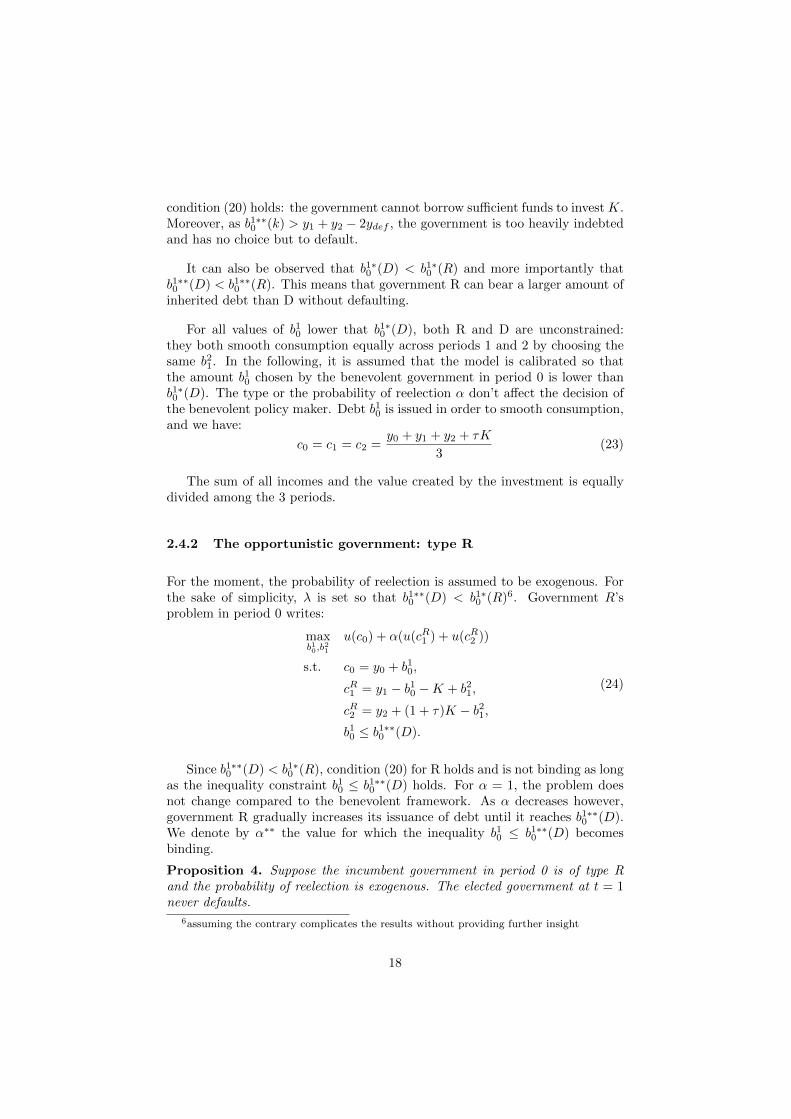
00(�) � 0 such that, for all ↵ thatbelongs to [0;↵00(�)], government D defaults if it is elected. Also, ↵00(�) is nondecreasing and for � su�ciently large, ↵00(�) > 0.
The proof can be found in the appendix. When ↵ is lower than ↵
00(�), Gov-ernment R chooses to issue more than b
1⇤⇤0 (D) in order to make the probability
of reelection jump to ↵. Default happens only because government R has thepower to modify the probability of reelection with its issuance of debt.
Figure 6: The occurrence of political default - opportunistic incumbent R
0 10
0.5
1
1.5
2
2.5
3
α
Vpay
Vdef
with λ=1
Vdef
with λ=0.3
α′ ′(0.3) α
′ ′(1) α Cond. (27)
Note: This figure assumes (y0, y1, y2) = (1.5, 2, 2), ydef = 1.5, K = 1.5, ⌧ = 1.3. Vdef
denotes the value function when government R issues more than b1⇤⇤0 (D): defaults occurs if
government D is elected. Vpay denotes the value function when government R respects the
constraint b0 b1⇤⇤0 (D)
20
2.4.3 The opportunistic government: type D
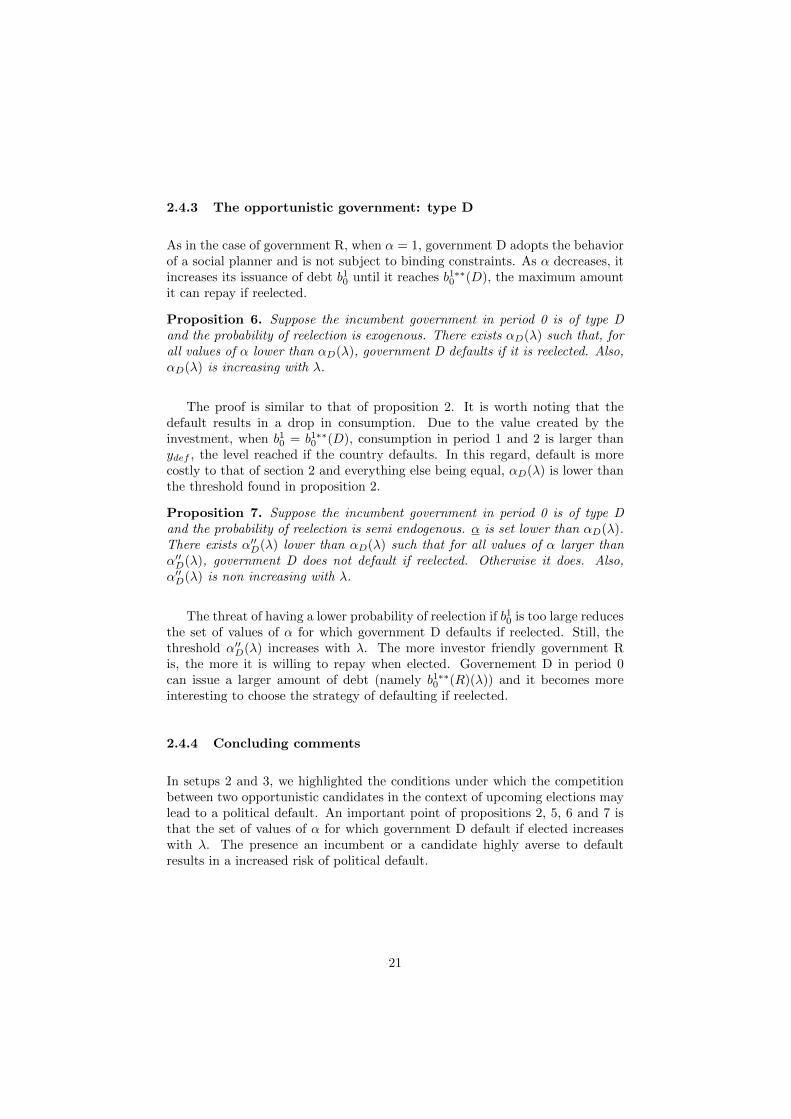
As in the case of government R, when ↵ = 1, government D adopts the behaviorof a social planner and is not subject to binding constraints. As ↵ decreases, itincreases its issuance of debt b10 until it reaches b1⇤⇤0 (D), the maximum amountit can repay if reelected.
Proposition 6. Suppose the incumbent government in period 0 is of type Dand the probability of reelection is exogenous. There exists ↵D(�) such that, forall values of ↵ lower than ↵D(�), government D defaults if it is reelected. Also,↵D(�) is increasing with �.
The proof is similar to that of proposition 2. It is worth noting that thedefault results in a drop in consumption. Due to the value created by theinvestment, when b
10 = b
1⇤⇤0 (D), consumption in period 1 and 2 is larger than
ydef , the level reached if the country defaults. In this regard, default is morecostly to that of section 2 and everything else being equal, ↵D(�) is lower thanthe threshold found in proposition 2.
Proposition 7. Suppose the incumbent government in period 0 is of type Dand the probability of reelection is semi endogenous. ↵ is set lower than ↵D(�).There exists ↵
00D(�) lower than ↵D(�) such that for all values of ↵ larger than
↵
00D(�), government D does not default if reelected. Otherwise it does. Also,
↵
00D(�) is non increasing with �.
The threat of having a lower probability of reelection if b10 is too large reducesthe set of values of ↵ for which government D defaults if reelected. Still, thethreshold ↵
00D(�) increases with �. The more investor friendly government R
is, the more it is willing to repay when elected. Governement D in period 0can issue a larger amount of debt (namely b
1⇤⇤0 (R)(�)) and it becomes more
interesting to choose the strategy of defaulting if reelected.
2.4.4 Concluding comments
In setups 2 and 3, we highlighted the conditions under which the competitionbetween two opportunistic candidates in the context of upcoming elections maylead to a political default. An important point of propositions 2, 5, 6 and 7 isthat the set of values of ↵ for which government D default if elected increaseswith �. The presence an incumbent or a candidate highly averse to defaultresults in a increased risk of political default.
21
Figure 7: The occurrence of political default - opportunistic incumbent D
0 11
1.2
1.4
1.6
1.8
2
2.2
2.4
2.6
2.8
Vpay
Vdef
with λ=0.4
α α ′ ′
D(λ ) αD(λ )
Note: This figure assumes (y0, y1, y2) = (1.5, 2, 2), ydef = 1.5, K = 1.5, ⌧ = 1.3 and � = 0.4.Vdef denotes the value function when government D issues more than b1⇤⇤0 (D): defaults occurs
it is reelected. Vpay denotes the value function when government D respects the constraint
b0 b1⇤⇤0 (D)
3 The maturity composition of debt in pre-electionperiods: empirical evidence
The objective of this section is to test empirically the main implications high-lighted in the first setup of our model. Under the benevolent specification, weproved that the maturity structure of debt in pre-election periods essentially de-pends on the type of the government that is expected to win the election, whilethe type of the incumbent government is of no relevance. By contrast, when itis assumed that governments are opportunistic, the choice of the optimal ma-turity structure is driven by the type of the incumbent government, while theprobability of reelection accounts for the extent of the impact observed. Moreformally, we test the two following hypotheses7:
7We justify below why the political orientation is used as a proxy for the government’s
type
22
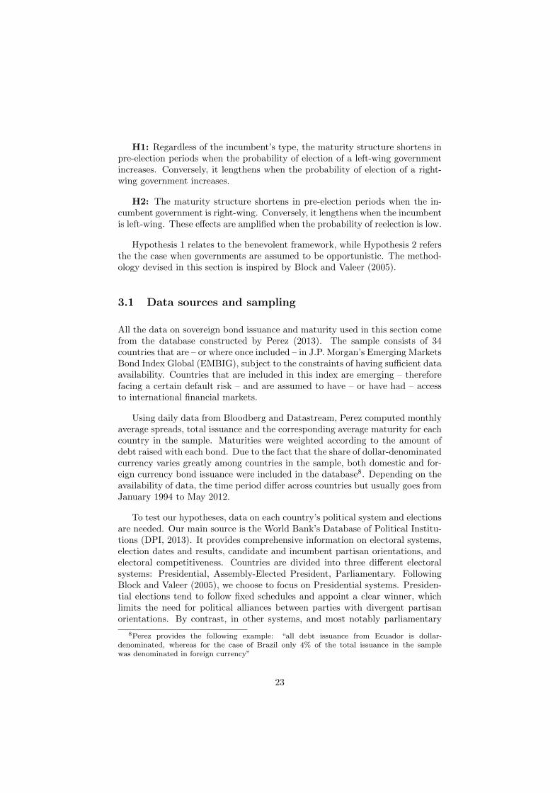
H1: Regardless of the incumbent’s type, the maturity structure shortens inpre-election periods when the probability of election of a left-wing governmentincreases. Conversely, it lengthens when the probability of election of a right-wing government increases.
H2: The maturity structure shortens in pre-election periods when the in-cumbent government is right-wing. Conversely, it lengthens when the incumbentis left-wing. These e↵ects are amplified when the probability of reelection is low.
Hypothesis 1 relates to the benevolent framework, while Hypothesis 2 refersthe the case when governments are assumed to be opportunistic. The method-ology devised in this section is inspired by Block and Valeer (2005).
3.1 Data sources and sampling
All the data on sovereign bond issuance and maturity used in this section comefrom the database constructed by Perez (2013). The sample consists of 34countries that are – or where once included – in J.P. Morgan’s Emerging MarketsBond Index Global (EMBIG), subject to the constraints of having su�cient dataavailability. Countries that are included in this index are emerging – thereforefacing a certain default risk – and are assumed to have – or have had – accessto international financial markets.
Using daily data from Bloodberg and Datastream, Perez computed monthlyaverage spreads, total issuance and the corresponding average maturity for eachcountry in the sample. Maturities were weighted according to the amount ofdebt raised with each bond. Due to the fact that the share of dollar-denominatedcurrency varies greatly among countries in the sample, both domestic and for-eign currency bond issuance were included in the database8. Depending on theavailability of data, the time period di↵er across countries but usually goes fromJanuary 1994 to May 2012.
To test our hypotheses, data on each country’s political system and electionsare needed. Our main source is the World Bank’s Database of Political Institu-tions (DPI, 2013). It provides comprehensive information on electoral systems,election dates and results, candidate and incumbent partisan orientations, andelectoral competitiveness. Countries are divided into three di↵erent electoralsystems: Presidential, Assembly-Elected President, Parliamentary. FollowingBlock and Valeer (2005), we choose to focus on Presidential systems. Presiden-tial elections tend to follow fixed schedules and appoint a clear winner, whichlimits the need for political alliances between parties with divergent partisanorientations. By contrast, in other systems, and most notably parliamentary
8Perez provides the following example: “all debt issuance from Ecuador is dollar-
denominated, whereas for the case of Brazil only 4% of the total issuance in the sample
was denominated in foreign currency”
23
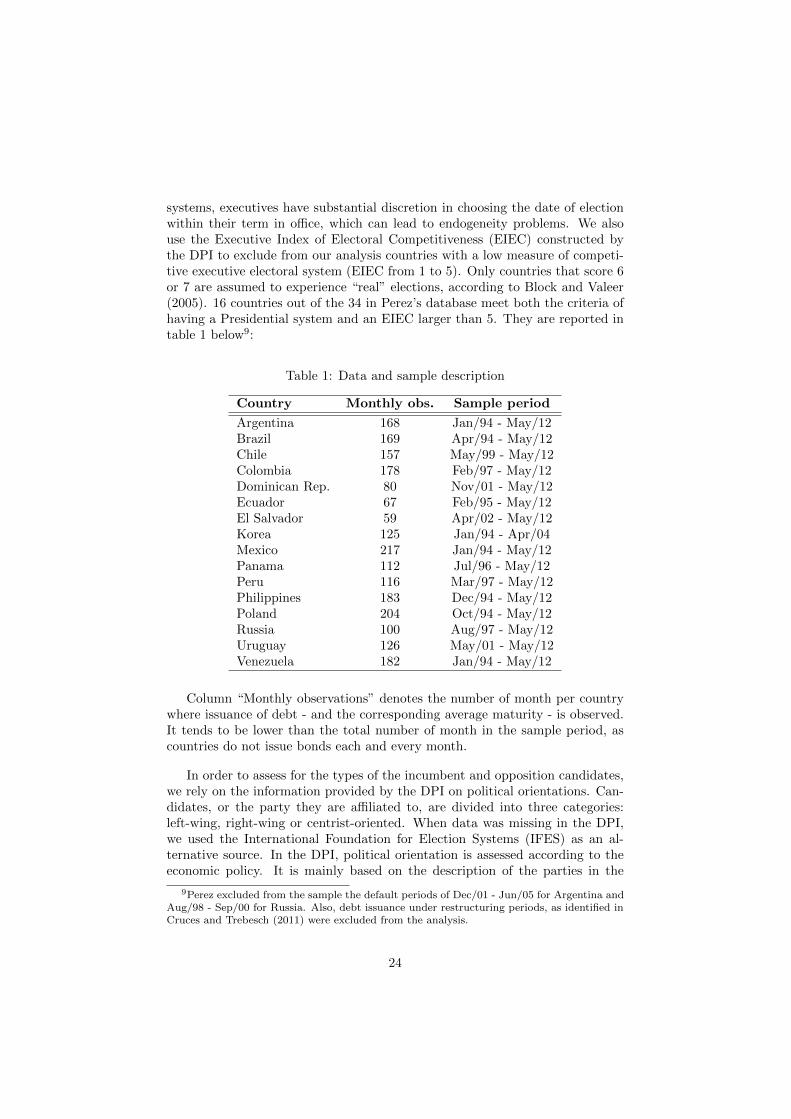
systems, executives have substantial discretion in choosing the date of electionwithin their term in o�ce, which can lead to endogeneity problems. We alsouse the Executive Index of Electoral Competitiveness (EIEC) constructed bythe DPI to exclude from our analysis countries with a low measure of competi-tive executive electoral system (EIEC from 1 to 5). Only countries that score 6or 7 are assumed to experience “real” elections, according to Block and Valeer(2005). 16 countries out of the 34 in Perez’s database meet both the criteria ofhaving a Presidential system and an EIEC larger than 5. They are reported intable 1 below9:
Table 1: Data and sample description
Country Monthly obs. Sample period
Argentina 168 Jan/94 - May/12Brazil 169 Apr/94 - May/12Chile 157 May/99 - May/12Colombia 178 Feb/97 - May/12Dominican Rep. 80 Nov/01 - May/12Ecuador 67 Feb/95 - May/12El Salvador 59 Apr/02 - May/12Korea 125 Jan/94 - Apr/04Mexico 217 Jan/94 - May/12Panama 112 Jul/96 - May/12Peru 116 Mar/97 - May/12Philippines 183 Dec/94 - May/12Poland 204 Oct/94 - May/12Russia 100 Aug/97 - May/12Uruguay 126 May/01 - May/12Venezuela 182 Jan/94 - May/12
Column “Monthly observations” denotes the number of month per countrywhere issuance of debt - and the corresponding average maturity - is observed.It tends to be lower than the total number of month in the sample period, ascountries do not issue bonds each and every month.
In order to assess for the types of the incumbent and opposition candidates,we rely on the information provided by the DPI on political orientations. Can-didates, or the party they are a�liated to, are divided into three categories:left-wing, right-wing or centrist-oriented. When data was missing in the DPI,we used the International Foundation for Election Systems (IFES) as an al-ternative source. In the DPI, political orientation is assessed according to theeconomic policy. It is mainly based on the description of the parties in the
9Perez excluded from the sample the default periods of Dec/01 - Jun/05 for Argentina and
Aug/98 - Sep/00 for Russia. Also, debt issuance under restructuring periods, as identified in
Cruces and Trebesch (2011) were excluded from the analysis.
24
sources (content of party names, judgments by academic and professional com-mentators). Criteria used by Beck et al. (2001) to locate parties on the politicalspectrum suggest that right-wing and centrist parties, by contrast with left-wingparties, advocate creditor-friendly policies. Our main assumption is that theright-wing and the few centrist-oriented governments in the sample correspondto the government of type R of our model, while left-wing governments are oftype D.
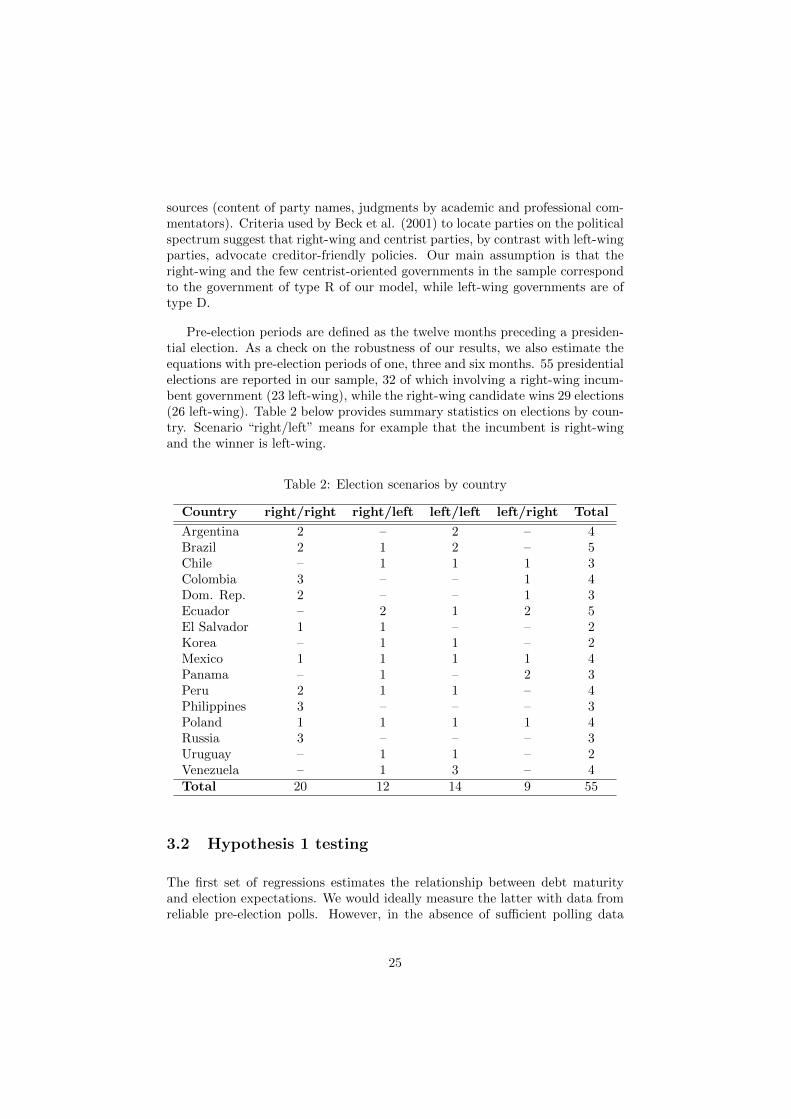
Pre-election periods are defined as the twelve months preceding a presiden-tial election. As a check on the robustness of our results, we also estimate theequations with pre-election periods of one, three and six months. 55 presidentialelections are reported in our sample, 32 of which involving a right-wing incum-bent government (23 left-wing), while the right-wing candidate wins 29 elections(26 left-wing). Table 2 below provides summary statistics on elections by coun-try. Scenario “right/left” means for example that the incumbent is right-wingand the winner is left-wing.
Table 2: Election scenarios by country
Country right/right right/left left/left left/right Total
Argentina 2 – 2 – 4Brazil 2 1 2 – 5Chile – 1 1 1 3Colombia 3 – – 1 4Dom. Rep. 2 – – 1 3Ecuador – 2 1 2 5El Salvador 1 1 – – 2Korea – 1 1 – 2Mexico 1 1 1 1 4Panama – 1 – 2 3Peru 2 1 1 – 4Philippines 3 – – – 3Poland 1 1 1 1 4Russia 3 – – – 3Uruguay – 1 1 – 2Venezuela – 1 3 – 4Total 20 12 14 9 55
3.2 Hypothesis 1 testing
The first set of regressions estimates the relationship between debt maturityand election expectations. We would ideally measure the latter with data fromreliable pre-election polls. However, in the absence of su�cient polling data
25
availability for most of the countries in our sample, we follow Block and Valeerby using actual final election results retrospectively. This method relies on theassumption that pre-election views are generally not upset by actual election-dayresults. Consequently, there is no divergence of expectations between creditorsand the incumbent government, which fits with the framework of our model.
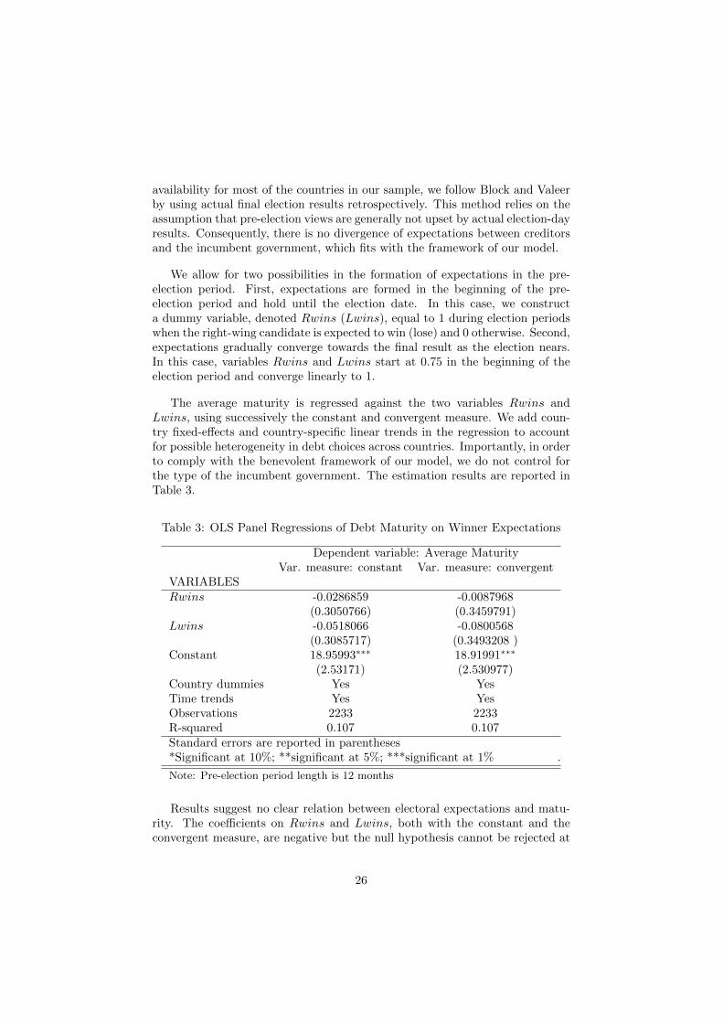
We allow for two possibilities in the formation of expectations in the pre-election period. First, expectations are formed in the beginning of the pre-election period and hold until the election date. In this case, we constructa dummy variable, denoted Rwins (Lwins), equal to 1 during election periodswhen the right-wing candidate is expected to win (lose) and 0 otherwise. Second,expectations gradually converge towards the final result as the election nears.In this case, variables Rwins and Lwins start at 0.75 in the beginning of theelection period and converge linearly to 1.
The average maturity is regressed against the two variables Rwins andLwins, using successively the constant and convergent measure. We add coun-try fixed-e↵ects and country-specific linear trends in the regression to accountfor possible heterogeneity in debt choices across countries. Importantly, in orderto comply with the benevolent framework of our model, we do not control forthe type of the incumbent government. The estimation results are reported inTable 3.
Table 3: OLS Panel Regressions of Debt Maturity on Winner Expectations
Dependent variable: Average MaturityVar. measure: constant Var. measure: convergent
VARIABLESRwins -0.0286859 -0.0087968
(0.3050766) (0.3459791)Lwins -0.0518066 -0.0800568
(0.3085717) (0.3493208 )Constant 18.95993⇤⇤⇤ 18.91991⇤⇤⇤
(2.53171) (2.530977)Country dummies Yes YesTime trends Yes YesObservations 2233 2233R-squared 0.107 0.107Standard errors are reported in parentheses*Significant at 10%; **significant at 5%; ***significant at 1% .
Note: Pre-election period length is 12 months
Results suggest no clear relation between electoral expectations and matu-rity. The coe�cients on Rwins and Lwins, both with the constant and theconvergent measure, are negative but the null hypothesis cannot be rejected at
26
any commonly acceptable significance levels10. Therefore, Hypothesis 1 is re-jected by our results, which indicates that the benevolent framework alone is notenough to account for changes in bond maturity structure during pre-electionperiods.
3.3 Hypothesis 2 testing
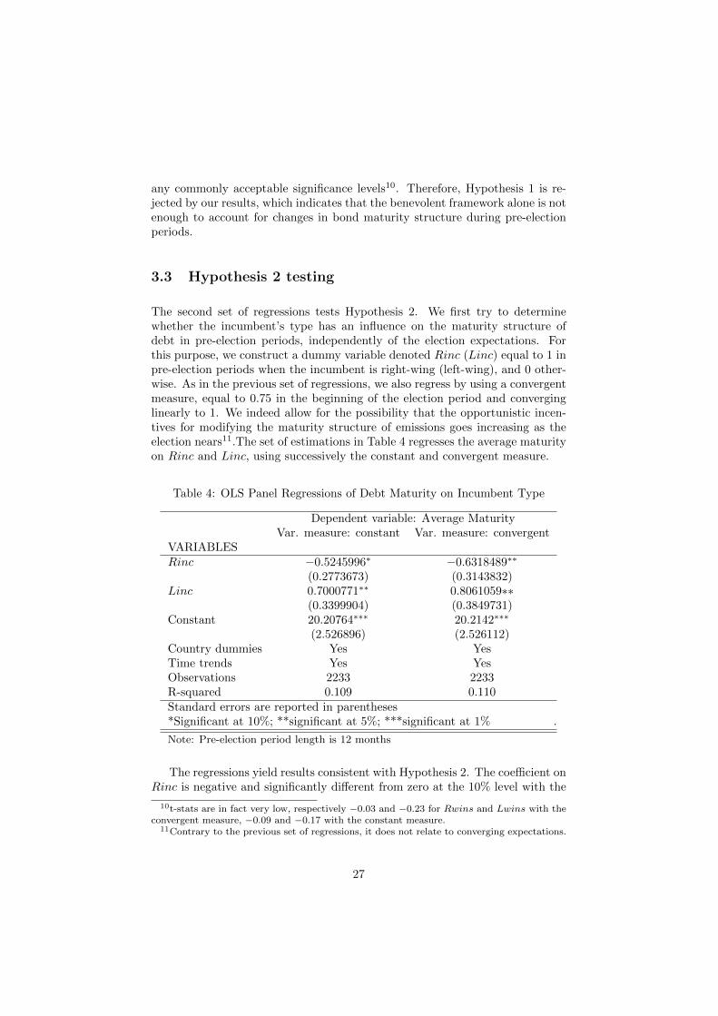
The second set of regressions tests Hypothesis 2. We first try to determinewhether the incumbent’s type has an influence on the maturity structure ofdebt in pre-election periods, independently of the election expectations. Forthis purpose, we construct a dummy variable denoted Rinc (Linc) equal to 1 inpre-election periods when the incumbent is right-wing (left-wing), and 0 other-wise. As in the previous set of regressions, we also regress by using a convergentmeasure, equal to 0.75 in the beginning of the election period and converginglinearly to 1. We indeed allow for the possibility that the opportunistic incen-tives for modifying the maturity structure of emissions goes increasing as theelection nears11.The set of estimations in Table 4 regresses the average maturityon Rinc and Linc, using successively the constant and convergent measure.
Table 4: OLS Panel Regressions of Debt Maturity on Incumbent Type
Dependent variable: Average MaturityVar. measure: constant Var. measure: convergent
VARIABLESRinc �0.5245996⇤ �0.6318489⇤⇤
(0.2773673) (0.3143832)Linc 0.7000771⇤⇤ 0.8061059⇤⇤
(0.3399904) (0.3849731)Constant 20.20764⇤⇤⇤ 20.2142⇤⇤⇤
(2.526896) (2.526112)Country dummies Yes YesTime trends Yes YesObservations 2233 2233R-squared 0.109 0.110Standard errors are reported in parentheses*Significant at 10%; **significant at 5%; ***significant at 1% .
Note: Pre-election period length is 12 months
The regressions yield results consistent with Hypothesis 2. The coe�cient onRinc is negative and significantly di↵erent from zero at the 10% level with the
10t-stats are in fact very low, respectively �0.03 and �0.23 for Rwins and Lwins with the
convergent measure, �0.09 and �0.17 with the constant measure.
11Contrary to the previous set of regressions, it does not relate to converging expectations.
27
constant measure, at the 5% level with the convergent measure; The coe�cienton Linc is positive and significantly di↵erent from zero at the 5% level withboth measures. Interestingly, the convergent measure yields larger and morerobust coe�cients, suggesting that the opportunistic incentives for modifyingthe maturity structure of emissions does increase as the election nears. We alsocheck the robustness of these measures by re-estimating these equations withpre–election periods of one, three and six months. The results are reported inAppendix 2. As the number of observations is lower when pre-election periodsare assumed to be shorter, the estimations are less accurate. However ,we dofind negative coe�cients for Rinc and positive coe�cients for Linc, which onceagain matches the predictions of our model.
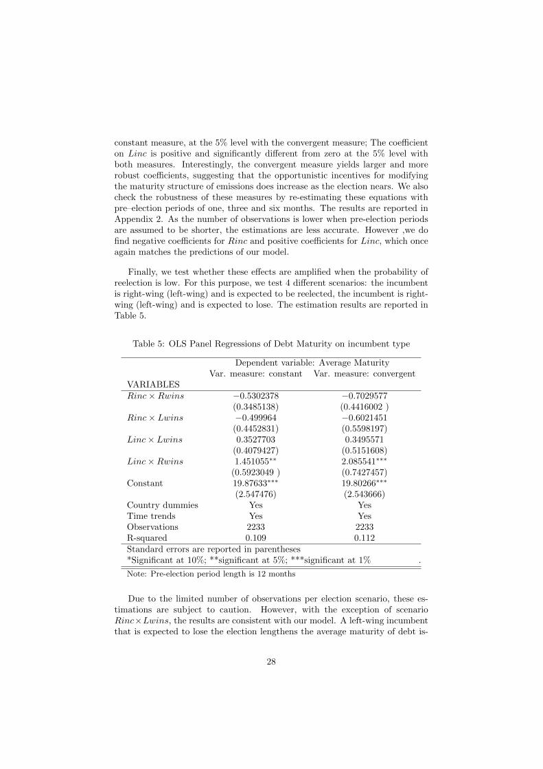
Finally, we test whether these e↵ects are amplified when the probability ofreelection is low. For this purpose, we test 4 di↵erent scenarios: the incumbentis right-wing (left-wing) and is expected to be reelected, the incumbent is right-wing (left-wing) and is expected to lose. The estimation results are reported inTable 5.
Table 5: OLS Panel Regressions of Debt Maturity on incumbent type
Dependent variable: Average MaturityVar. measure: constant Var. measure: convergent
VARIABLESRinc⇥Rwins �0.5302378 �0.7029577
(0.3485138) (0.4416002 )Rinc⇥ Lwins �0.499964 �0.6021451
(0.4452831) (0.5598197)Linc⇥ Lwins 0.3527703 0.3495571
(0.4079427) (0.5151608)Linc⇥Rwins 1.451055⇤⇤ 2.085541⇤⇤⇤
(0.5923049 ) (0.7427457)Constant 19.87633⇤⇤⇤ 19.80266⇤⇤⇤
(2.547476) (2.543666)Country dummies Yes YesTime trends Yes YesObservations 2233 2233R-squared 0.109 0.112Standard errors are reported in parentheses*Significant at 10%; **significant at 5%; ***significant at 1% .
Note: Pre-election period length is 12 months
Due to the limited number of observations per election scenario, these es-timations are subject to caution. However, with the exception of scenarioRinc⇥Lwins, the results are consistent with our model. A left-wing incumbentthat is expected to lose the election lengthens the average maturity of debt is-
28
sued by 1.45 years (significant at the 5% level) with the constant measure, andby 2.09 years (significant at the 1% level) with the convergent measure. Bothtypes of government do not significantly change the maturity structure of theirissuances when they expect to be reelected.
3.4 Concluding comments
In summary, we found that electoral expectations, taken alone, have no signifi-cant impact on maturity. Controlling for the type of the incumbent governmentis needed to get more conclusive results. We showed that the maturity structureshortens in pre-election periods when the incumbent government is right-wing.Conversely, it lengthens when the incumbent is left-wing, and this e↵ect is am-plified when its probability of reelection is low. The analysis therefore tendsto show that the opportunistic nature of policy makers predominates over theirbenevolent nature.
29
4 Conclusion
In this paper, we developed a simple three-period model of political default toidentify the main determinants of the maturity structure of sovereign bond is-suances in pre-election periods and the conditions under which the competitionbetween two opportunistic candidates may trigger a default. Our findings on thematurity structure are that (i) a benevolent government set the maturity struc-ture in order to complete markets in the absence of state-contingent contracts,(ii) an opportunistic investor-friendly government strictly favors short-term debtbecause it can refinance it at a high price after the election, (iii) an opportunis-tic debtor-friendly government strictly favors long-term debt in order to avoidcostly refinancing if reelected. Endogenizing the decision of default, we provedthat a political default may happen when (i) an opportunistic debtor-friendlygovernment is unexpectedly reelected, (ii) an opportunistic creditor-friendly gov-ernment issues extensive quantities of debt in order to increase its probabilityof reelection but eventually loses.
The empirical analysis carried out on 55 presidential elections in 16 finan-cially integrated emerging countries suggest that the observed average maturityof issuances in pre-election periods follow the predictions of our model underthe opportunistic framework.
However, the limited number of observations make these results subject tocaution. Further analysis needs to be done on a larger sample of elections toattest to the robustness of our results. This would also allow to test more specificscenarios, for example whether a victory is widely expected or uncertain owingto closely balanced expectations.
30
References
[1] Aguiar, M. and G. Gopinath (2006). “Defaultable Debt, Interest Ratesand the Current Account.” Journal of International Economics 69 (June):64?83.
[2] Alfaro, L. and F. Kanczuk (2005). “Sovereign Debt as a ContingentClaim: A Quantitative Approach.” Journal of International Economics65 (March): 297?314.
[3] Amador, M. (2003). “A Political Economy Model of Sovereign Debt Re-payment.” Stanford University mimeo.
[4] Arellano, C. (2008). “Default Risk and Income Fluctuations in EmergingEconomies.” American Economic Review 98 (June): 690?712.
[5] Arellano, C. and A. Ramanarayanan (2012, revised 2013). “Default andthe Maturity Structure of Sovereign Bonds.” Journal of Political Economy,120(2): 187-232.
[6] Bi, R. (2006). “Debt Dilution and the Maturity Structure of SovereignBonds”. Manuscript, University of Maryland.
[7] Block, S. and P. Vaaler (2005). “Counting the investor vote: political busi-ness cycle e↵ects on sovereign bond spreads in developing countries.” Jour-nal of International Business Studies, vol. 36(1), pages 62-88, January.
[8] Buera, F. and J. P. Nicolini (2004). “Optimal Maturity of GovernmentDebt without State Contingent Bonds.” Journal of Monetary Economics,51(3): 531-554.
[9] Cole, H. L., Dow, J. and W. B. English (1995). “Default, Settlement,and Signalling: Lending Resumption in a Reputational Model of SovereignDebt.” International Economic Review 36 (May): 365?85.
[10] Cuadra, G. and H. Sapriza (2008). “Sovereign Default, Interest Rates andPolitical Uncertainty in Emerging Markets.” Journal of International Eco-nomics 76 (September): 78?88.
[11] Jeanne, O. (2009). “Debt Maturity and the International Financial Archi-tecture.” American Economic Review, 99(5): 2135-2148.
[12] Hatchondo, J. C., Martinez, L. and H. Sapriza (2009). “HeterogeneousBorrowers in Quantitative Models of Sovereign Default.” International Eco-nomic Review 50 (October): 1,129?51.
[13] Hatchondo, J. C., Martinez, L., and C. Sosa Padilla (2010). “Debt dilutionand sovereign default risk.” Federal Reserve Bank of Richmond WorkingPaper 10-08R.
31
[14] Miller, V. (1997), “Political Instability and Debt Maturity.” Economic In-quiry, vol. XXXV, January 1997, 12-27.
[15] Perez, D. (2013). “Sovereign Debt Maturity Structure Under Asymmet-ric Information.” Available at SSRN: http://ssrn.com/abstract=2383640or http://dx.doi.org/10.2139/ssrn.2383640
[16] Rodrik, D. and A. Velazco (1999). “Short Term Capital Flows.” In AnnualWorld Bank Conference on Development Economics, Washington, D.C.:World Bank.
[17] Tirole, J. (2003). “Ine�cient Foreign Borrowing: A Dual- and Common-Agency Perspective.” American Economic Review, 93(5): 1678-1702.
[18] Tomz, M. and Mark L. J. Wright (2007). “Do Countries Default in BadTimes?” Journal of the European Economic Association 5 : 352?60.
32
APPENDIX 1
This appendix provides the proofs of proposition 1 to 5.
Proof of proposition 1. Suppose that there exists ↵ such that it is optimal forgovernment R to borrow more than what government D is willing to repay. Bysetting b
10 = y1 � ydef , short-term debt can still be issued at price 1 as default
will only occur in period 2. The maximization problem becomes:
maxb20
u(c0) + ↵[u(cR1 ) + u(cR2 )]
s.t. c0 = y0 + y1 � ydef + ↵b
20
c
R1 = c
R2 = (y2 + ydef � b
20)/2
(30)
We abstract from the two inequality constraints. The first order conditiongives u0(c0) = u
0(c1) = u
0(c2), so the government wants to smooth consumptionequally across periods. But as it borrows in period 0 at a low price ↵, thelevel of consumption reached in each period is lower than (y0 + y1 + y2)/3,the consumption reached with the benevolent strategy, which is itself strictlydominated by the strategy of borrowing b0 = y1 + y2 � 2ydef when ↵ is lowerthan ↵
0. So government R never borrows more than what government D canrepay if it is reelected. This proves proposition 1
Proof of proposition 2. For values of ↵ equal or lower than ↵
0, government Dcan choose between two strategies. First, it can borrow b0 = y1 + y2 � 2ydef atprice 1 and repay if it is reelected, with c
D1 = c
D2 = ydef . Second, it can borrow
b0 = y1 + y2 � 2(1 � �)ydef at price 1 � ↵ and then default, so c
D1 and c
D2 are
also equal to ydef . As consumption in periods 1 and 2 are the same in bothcases, government D chooses the strategy that maximizes the amount it can getto consume in period 0. The second strategy is optimal as soon as:
⇢y1 + y2 � 2ydef<(1� ↵)(y1 + y2 � 2(1� �)ydef )
↵ < ↵
0
This system simplifies to:
↵ < min
2�ydef
y1 + y2 � 2(1� �)ydef;↵0
�(31)
The left hand side corresponds to ↵
00(�). For values of � such that ↵00(�) =2�ydef
y1+y2�2(1��)ydef, we di↵erentiate and find:
33

(↵00)0(�) =2ydef (y1 + y2)� 4y2def
(y1 + y2 � 2(1� �)ydef )2(32)
As y1 and y2 are larger than ydef , we get ↵0(�) > 0 and ↵
2 is increasing in�.
This proves proposition 2.
Proof of proposition 3. The proof is solved for government D, so �k = 0. Fortype R, you just have to replace ydef by (1� �R)ydef in the following.
We first need to find b
1⇤0 , the amount of inherited debt for which condition
(20) becomes binding. When government k is unconstrained in period 1, itperfectly smoothes consumption between t = 1 and t = 2. Starting from c1 = c2,we find:
b
21 =
y1 + y2 + ⌧K � b
10
2� (y1 � b
10 �K) (33)
Using this expression and u = log, condition (21) rewrites:
✓y1 + y2 + ⌧K � b
10
2
◆2
�✓y1 + y2 + ⌧K � b
10
2+K
◆ydef � 0 (34)
We find the determinant of this quadratic equation, which is 16Kydef+4y2def .This gives:
b
1⇤0 =
2y1 + 2y2 + 2⌧K � 2ydef +q
16Kydef + 4y2def
2(35)
Simplifying, we get the desired expression for b1⇤0
We now want to find b
1⇤⇤0 , the value above which no b
21 can make condition
(20) verified. Using again u = log, condition (20) rewrites:
(y1 � b
10 + b
21 �K)(y2 � b
21 + (1 + ⌧)K)� (y1 � b
10 + b
21)ydef � 0 (36)
Considering b
21 as the variable, this is the equation of an inverse parabolic
curve. We find the determinant:
(y1 � b
10)
2 + (2y2 � 2ydef + 2⌧K)(y1 � b
10)
+ [(y2)2 + (ydef )
2 � 2(2 + ⌧)Kydef + 2⌧Ky2 � 2y2ydef + (⌧K)2] (37)
34

The determinant is itself a quadratic equation, now with respect to b
10. Our
objective is to find the value of b10 for which this expression is equal to 0. Thedeterminant of this new quadratic equation is 16Kydef , and we find:
y1 � b
1⇤⇤0 =
�2(y2 � ydef + ⌧K) +p16Kydef
2(38)
Simplifying, we get the desired expression for b1⇤⇤0
For values of b10 above b1⇤⇤0 , condition (20) cannot hold because the equationin (36) is negative for all values of b21. As b1⇤⇤0 > y1+y2�2ydef , the governmentcannot repay and immediately defaults.
This proves proposition 3
Proof of proposition 4. The proof is similar to that of proposition 1. By issuingmore than b
1⇤⇤0 (D), the maximization problem becomes:
maxb10,b
21
u(c0) + ↵(u(cR1 ) + u(cR2 ))
s.t. c0 = y0 + ↵b
10,
c
R1 = y1 � b
10 �K + b
21,
c
R2 = y2 + (1 + ⌧)K � b
21,
b
10 b
1⇤⇤0 (R),
(39)
The first order conditions give c0 = c
R2 = c
R2 . This strategy is strictly
dominated by the benevolent strategy. The latter also enables to smooth con-sumption equally across periods but a larger level of consumption is reachedbecause debt is emitted in period 0 at price 1 instead of ↵. So the governmentnever borrows more than b
1⇤⇤0 (D), and the elected government at t = 1 never
defaults.
This proves proposition 4
Proof of proposition 5. Using assumptions 1 and 2 and the fact that Vdef iscontinuous increasing, we get that: Vdef,�=1(↵) > Vpay(0). As Vpay is alsocontinuous increasing, we find that there exists ↵
00(1) such that, for all ↵ in[0;↵00(1)[, we have Vdef,�=1(↵) > Vpay(↵). In that case, government R is bettero↵ by issuing more debt than b
1⇤⇤0 (D). If government D is elected in period 1
(with probability 1� ↵), it will default surely.
35
We define �̄(↵) such that for all � in [�̄(↵); 1], the government is uncon-strained, that is Vdef,���̄(↵)(↵) = Vdef,�=1(↵). So ↵
00(�) is constant on [�̄(↵); 1].
For values of � lower than �̄(↵), the government is constrained. As � decreases,VD,�(↵) continuously decreases, and so does ↵00(�) until VD,�(↵) = VR(0) or b10hits the limit b
1⇤⇤0 (R)(�). We call this threshold �(↵). For values of � lower
than �(↵), ↵00(�) is equal to 0. Government D, if elected, does not default.
This proves proposition 5
36
APPENDIX 2
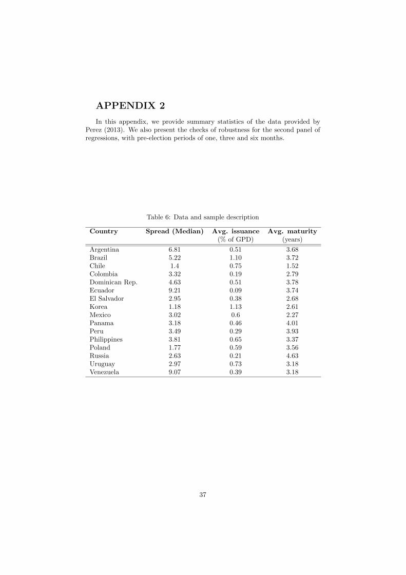
In this appendix, we provide summary statistics of the data provided byPerez (2013). We also present the checks of robustness for the second panel ofregressions, with pre-election periods of one, three and six months.
Table 6: Data and sample description
Country Spread (Median) Avg. issuance Avg. maturity(% of GPD) (years)
Argentina 6.81 0.51 3.68Brazil 5.22 1.10 3.72Chile 1.4 0.75 1.52Colombia 3.32 0.19 2.79Dominican Rep. 4.63 0.51 3.78Ecuador 9.21 0.09 3.74El Salvador 2.95 0.38 2.68Korea 1.18 1.13 2.61Mexico 3.02 0.6 2.27Panama 3.18 0.46 4.01Peru 3.49 0.29 3.93Philippines 3.81 0.65 3.37Poland 1.77 0.59 3.56Russia 2.63 0.21 4.63Uruguay 2.97 0.73 3.18Venezuela 9.07 0.39 3.18
37
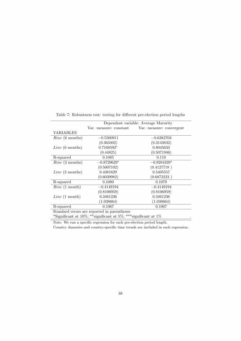
Table 7: Robustness test: testing for di↵erent pre-election period lengths
Dependent variable: Average MaturityVar. measure: constant Var. measure: convergent
VARIABLESRinc (6 months) �0.5560911 �0.6382703
(0.363402) (0.3143832)Linc (6 months) 0.7168592⇤ 0.8045633
(0.44825) (0.5071946)R-squared 0.1085 0.110Rinc (3 months) �0.8729629⇤ �0.9284339⇤
(0.5007102) (0.4127718 )Linc (3 months) 0.4381629 0.5405557
(0.6039982) (0.6872223 )R-squared 0.1080 0.1079Rinc (1 month) �0.4149194 �0.4149194
(0.8106959) (0.8106959)Linc (1 month) 0.3461236 0.3461236
(1.038664) (1.038664)R-squared 0.1067 0.1067Standard errors are reported in parentheses*Significant at 10%; **significant at 5%; ***significant at 1% .
Note: We run a specific regression for each pre-election period length.
Country dummies and country-specific time trends are included in each regression.
38