Sound-scapes for Robot Localisation through Dimensionality Reduction

Aaron S.W. Wong and Stephan K. Chalup

University of Newcastle, Australia

aaron.wong@studentmail.newcastle.edu.au

Abstract

Sound-scapes similar to landscapes, are geometric

representations of an objects’ relative positions in

the real world. In this paper we demonstrate how

to obtain and use a sound-scape to assist the Alde-

baran NAO with localisation. We apply dimension-

ality reduction techniques such as statistical learn-

ing methods which include neural networks, sup-

port vector machines, the recent graph based ap-

proximation technique isometric feature mapping

to extract the NAO’s field co-ordinate from its

recorded acoustic data. Results obtained includes

visualisations of sound-scapes (robot’s positions on

field) and positional accuracies of up to 80%.

1 Introduction

Robot localisation is an important feature for an intelligent

robot to make accurate decisions which primarily uses vision

based cues for localisation. In Robocup’s standard platform

league, robots are on a field which contains vision cues or

field objects such as goals beacons and field lines. However,

in this paper we explores dimensionality reduction techniques

for localisation purely based on sound-scape data.

Sound-scapes are useful for understanding our surrounding

environments in applications such as security, source tracking

or understanding human computer interaction. Accurate po-

sition or localisation information from sound-scape samples

consists of many channels of high dimensional acoustic data.

This high dimensional acoustic data is obtained by recording

real world sounds from the Aldebaran NAO robot.

As of 2008, the Aldebaran NAO was introduced to the mar-

ket as an entertainment robot, it is also replacing the Sony

AIBO in the standard platform league for Robocup. The NAO

has many advantages over the AIBO, such as better hardware

eg. 500 MHz AMD Geode processor, 25 degrees of freedom

for movement and standard Linux operating system [Gouail-

lier and Blazevic, 2006; Gouaillier et al., 2008].

Most importantly the NAO robot has more acoustic hard-

ware. This includes the option for four microphones and

stereo speakers (see Figure 1). Since the operating system is

based on Linux architecture, the software API currently uses

the powerful Advanced Sound Linux Architecture (ALSA)

libraries to record and obtain acoustic data from its array of

microphones [Gouaillier et al., 2008].

Figure 1: Profile of the NAO’s acoustic equipment: S1 and S2

denote speakers 1 and 2 respectively. Meanwhile M1, M2,

M3 and M4 denotes the microphones 1, 2, 3 and 4 respec-

tively. For the NAO Robocup edition, M2 and M4 are not

included.

This paper has been structured in the following manner.

Section 2 will discuss the traditional sound localisation tech-

niques and review past literature on these topics. Dimension-

ality reduction is discussed in section 3. Section 4 describes

the methodology which includes the process of obtaining the

sound-scape dataset, the experimental environment and tech-

niques used to obtain the results. Results from the exper-

iments will be presented in section 5, while section 6 will

generally discuss the method and the results. Finally, section

7 will present the conclusions.

2 Sound Localisation

Cues used for sound source localisation includes time differ-

ence of arrival and intensity difference between signals. Lo-

calisation though sound traditionally has exploited these two

cues directly which are effected strongly effected by noise

[Wang and Brown, 2006]. In the following subsections we

will discuss cues used for traditional sound source localisa-

tion and review some literature.

Inter-aural time difference

Angle of arrival estimation by inter-aural time difference or

time difference of arrival (TDoA), is a traditional technique

based on generalised cross-correlation to estimate the time

delay. It first appeared in [Knapp, 1976], however many

adaptations and extensions of this algorithm have been used

not only for sound source localisation but in various other

fields of signal processing, such as wireless sensor localisa-

tion, modelling of binaural hearing, robotics. Time difference

of arrival ∆t can be defined as a phase difference ∆φ:

∆t =∆φ

2πf(1)

where f is the frequency.

In [Huang et al., 2006] the authors used time difference of

arrival to calculate the angle of arrival from multiple sound

beacons positioned on the field. Triangulation was then ap-

plied to these cues to obtain the current position of the robot.

A similar method was used in [Li et al., 2007].

Inter-aural level difference

Intensity difference of arrival, or received signal strength,

also known as intensity or inter-aural level difference (ILD),

are used in many different applications. These applications

include wireless fidelity localisation, sound source localisa-

tion and human sound localisation. It is derived from ’inten-

sity difference theory’ for directional hearing, where this the-

ory implies that the received signals from microphones differ

from each other by an intensity difference relative to the extra

distance travelled by the sound signal.

The relation which best describe this property is that the

energy Ei(t) of the recorded signal s(t) is inversely propor-

tional to the distance squared:

Ei(t) =1

d2

i

∫

s(t)dt +

∫

ǫi(t)dt (2)

where di is the distance between the robots position and

sound source, and ǫi(t) is the noise. ILD was used by [Birch-

field and Gangishetty, 2005], where they present an algorithm

for obtaining sound source location using the intensity differ-

ence from microphone pairs.

3 Dimensionality Reduction

Dimensionality reduction techniques aim to obtain a low

dimensional representation for a given high dimensional

dataset. Recently statistical learning techniques have been

applied to acoustic datasets, not only for localisation, but also

for classification. These methods extract localisation infor-

mation from acoustic data by learning the mapping from high

dimensional data to its relevant lower dimensional represen-

tation.

Statistical learning techniques such as support vector ma-

chines have been applied to acoustic datasets for angle of

arrival localisation [Ben-Reuven and Singer, 2002; Murray

et al., 2005; Chen and Lai, 2005; Lei et al., 2006]. These

methods extract localisation information from acoustic data

by learning the mapping from high dimensional data to its

relevant lower dimensional representation.

Graph based dimensionality reduction technique is a gen-

eralised group for techniques such as PCA [Jolliffe, 1986],

MDS [Cox and Cox, 2001], Locally Linear Embedding[Saul and Roweis, 2003] used for obtaining a mapping from

high dimension to a lower dimension. In previous pilot

experiments with sound-scape data, isometric feature em-

bedding (ISOMAP) delivered promising results [Wong and

Chalup, 2008]. For this reason, the paper will concentrate on

ISOMAP.

In the following subsections we will discuss briefly the

statistical learning methods of neural networks and support

vector machines, and the graph approximation technique,

ISOMAP.

3.1 Neural Networks

A neural network consists of input, hidden, and output lay-

ers. The dimensionality of a original dataset can be denoted

by the number of nodes in the input layer, while the num-

ber of nodes in the output layer denotes the dimensionality of

the result [Haykin, 1999]. The hidden layers consist of nodes

which are weighted during training to learn a mapping from

the data points xi to its’ corresponding low dimensional rep-

resentation yi. Hidden nodes consists of an activation func-

tion; a linear activation function could be applied, where it be-

haves similarly to principal component analysis (PCA) [Jol-

liffe, 1986], while for non-linear applications, it is usually a

sigmoid function, [van der Maaten et al., 2007].

g(x) =1

1 + e−x(3)

Neural networks have been applied to varied range of ap-

plications, in regards to sound localisation it has been pre-

sented as a method to track and predict the movement of a

sound source with a degree of success [Murray et al., 2005].

3.2 Support Vector Machines

Support Vector Machines (SVM) consists of a linear clas-

sifier, extended by the kernel trick to enable classification

in high dimensional non-linear space [Scholkopf and Smola,

2002]. Kernelisation is achieved by the use of the ’kernel

trick’. The kernel trick is defined as follows: Assume a real

valued function k : ℜd ×ℜd → ℜ and there exists a mapping

Φ : ℜd → H into a dot product ’feature space’ H , such that

for all x, x′ ∈ ℜd we have:

Φ(x) · Φ(x′) = k(x, x′) (4)

where k(x, x′) is a non-linear similarity measure. This can

be though of as a substitution of the Euclidean dot product

space to a dot product of the feature space. The kernel gives

the property of non-linearity to PCA. There are many differ-

ent kernels available to be used, some include linear (PCA),

polynomial, radial basis function, etc.

SVM is based on maximum marginal separation through

the principal of structural risk minimisation using hyper-

planes. These hyperplanes create a linear decision or bound-

ary that optimally separates two classes, Assume we have

a dataset Xi ∈ ℜn, i = 1, . . . N , with associated labels

yi ∈ {−1, 1}. The goal is to find the separating hyperplane

with the maximum distance to the closest point of the train-

ing set and minimising the training errors. The optimal hy-

perplane is given as follows,

yi = xi · wo + b (5)

where yi is the low dimensional class representation of high

dimensional data sample xi, wo is the optimal norm to en-

able maximum separation between two classes and b is the

hyperplanes bias.

SVMs have also shown some success in the field of sound

localisation, with sound data used to create support vectors in

order to classify the angle of arrival from the recorded sound[Ben-Reuven and Singer, 2002; Chen and Lai, 2005; Lei et

al., 2006].

3.3 Isometric Feature Mapping

Isometric feature mapping (ISOMAP), a non-linear dimen-

sionality reduction technique, is an extension of MDS (ordi-

nal MDS [Tenenbaum, 1998] and classical MDS [Tenenbaum

et al., 2000]), where it attempts to preserve the geodesic dis-

tances between samples. Non-linear dimensionality reduc-

tion techniques have shown success in benchmark tasks such

as unfolding of the swiss roll and mapping of images on a sub-

manifold [Tenenbaum et al., 2000; Saul and Roweis, 2003].

ISOMAP was introduced by Tenenbaum et al. [Tenenbaum

et al., 2000] and consists of three steps:

1. Once a set of data is obtained we construct a nearest

neighbour graph G and weight each link in G by a

weighting function.

2. Then we compute the complete distance matrix for all

samples in G, using techniques such as Dijkstra’s algo-

rithm.

3. Finally, we use classical MDS to embed the data to a

lower dimension.

This structure leaves a few options open, such as alterna-

tives in the construction of the neighbourhood graph in G,

e.g. the number of nearest neighbours, k and the weighting

function. For this application and simplicity we choose to use

Euclidean distance as the weighting function and use k values

ranging from 1 to 100.

4 Methodology

This section will briefly describe the methodology undertaken

to achieve positioning through sound-scapes using sound bea-

cons on the NAO robot. Firstly, we will describe a sound-

scape sample followed by the the test field. Then we will dis-

cuss the method used to decode the NAO’s recorded sounds.

Finally, we will discuss techniques used to train and visualise

the NAO’s Position. An over all flow diagram of the system

is shown in Figure 2.

4.1 Sound-scape Sample

Different sounds are emitted by different objects on the

field, when recorded these combination of sounds creates

the sound-scape sample. To obtain a sound-scape sample,

we first created artificial chirps and assign them to different

sound beacons, where these sounds are emitted into the en-

vironment. The NAO robot then records the combination of

sounds to form its sound-scape sample (Fig. 3). These sound-

scape samples are unique to the NAO’s location due to acous-

tic propagation laws, such as time difference of arrival and

intensity level differences which are exploited in sound local-

isation.

Figure 3: Ideal Sound-scape Sample: An example of an ideal

sound-scape sample. There are two chirps emitted from B1,

the first chirp is to signify that the sound-scape sample is

about to begin.

4.2 Experimental Environment

The set up of the test field consists of a 270 × 210cm2 field

(Fig. 4). This field is located in an non-acoustically treated

room. Our co-ordinate system is in centimetres and is relative

to a corner of the field. Four sound beacons were arranged on

the field, B1 at co-ordinates (270, 210), B2 at co-ordinates

(270, 0), B3 at co-ordinates (0, 0), and B4 at co-ordinates

(0, 210). The NAO robot was placed at 48 locations on the

field, from (30, 30) to (270, 180) in intervals of 30cm in both

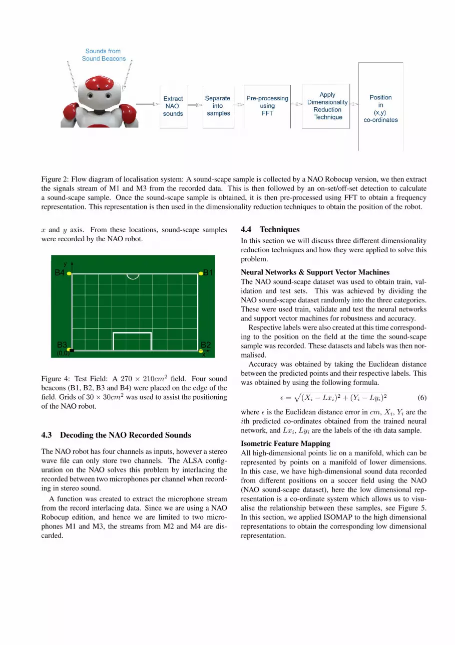
Figure 2: Flow diagram of localisation system: A sound-scape sample is collected by a NAO Robocup version, we then extract

the signals stream of M1 and M3 from the recorded data. This is then followed by an on-set/off-set detection to calculate

a sound-scape sample. Once the sound-scape sample is obtained, it is then pre-processed using FFT to obtain a frequency

representation. This representation is then used in the dimensionality reduction techniques to obtain the position of the robot.

x and y axis. From these locations, sound-scape samples

were recorded by the NAO robot.

Figure 4: Test Field: A 270 × 210cm2 field. Four sound

beacons (B1, B2, B3 and B4) were placed on the edge of the

field. Grids of 30 × 30cm2 was used to assist the positioning

of the NAO robot.

4.3 Decoding the NAO Recorded Sounds

The NAO robot has four channels as inputs, however a stereo

wave file can only store two channels. The ALSA config-

uration on the NAO solves this problem by interlacing the

recorded between two microphones per channel when record-

ing in stereo sound.

A function was created to extract the microphone stream

from the record interlacing data. Since we are using a NAO

Robocup edition, and hence we are limited to two micro-

phones M1 and M3, the streams from M2 and M4 are dis-

carded.

4.4 Techniques

In this section we will discuss three different dimensionality

reduction techniques and how they were applied to solve this

problem.

Neural Networks & Support Vector Machines

The NAO sound-scape dataset was used to obtain train, val-

idation and test sets. This was achieved by dividing the

NAO sound-scape dataset randomly into the three categories.

These were used train, validate and test the neural networks

and support vector machines for robustness and accuracy.

Respective labels were also created at this time correspond-

ing to the position on the field at the time the sound-scape

sample was recorded. These datasets and labels was then nor-

malised.

Accuracy was obtained by taking the Euclidean distance

between the predicted points and their respective labels. This

was obtained by using the following formula.

ǫ =√

(Xi − Lxi)2 + (Yi − Lyi)2 (6)

where ǫ is the Euclidean distance error in cm, Xi, Yi are the

ith predicted co-ordinates obtained from the trained neural

network, and Lxi, Lyi are the labels of the ith data sample.

Isometric Feature Mapping

All high-dimensional points lie on a manifold, which can be

represented by points on a manifold of lower dimensions.

In this case, we have high-dimensional sound data recorded

from different positions on a soccer field using the NAO

(NAO sound-scape dataset), here the low dimensional rep-

resentation is a co-ordinate system which allows us to visu-

alise the relationship between these samples, see Figure 5.

In this section, we applied ISOMAP to the high dimensional

representations to obtain the corresponding low dimensional

representation.

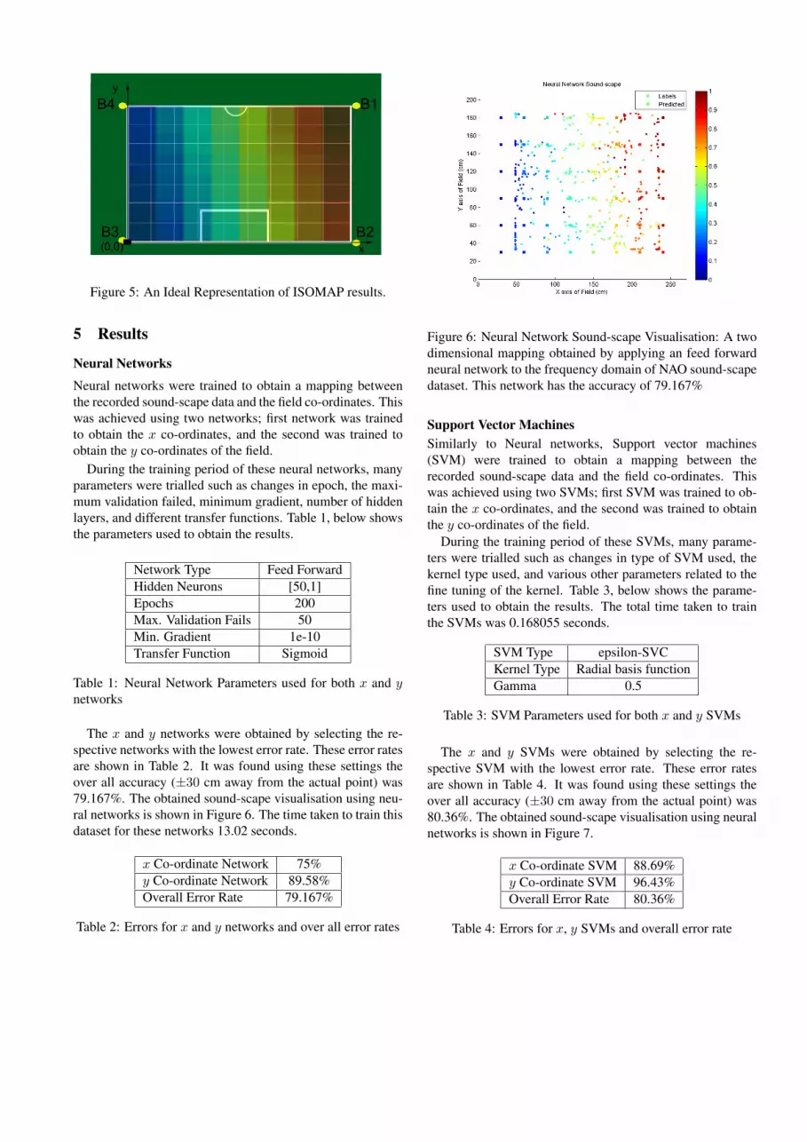
Figure 5: An Ideal Representation of ISOMAP results.

5 Results

Neural Networks

Neural networks were trained to obtain a mapping between

the recorded sound-scape data and the field co-ordinates. This

was achieved using two networks; first network was trained

to obtain the x co-ordinates, and the second was trained to

obtain the y co-ordinates of the field.

During the training period of these neural networks, many

parameters were trialled such as changes in epoch, the maxi-

mum validation failed, minimum gradient, number of hidden

layers, and different transfer functions. Table 1, below shows

the parameters used to obtain the results.

Network Type Feed Forward

Hidden Neurons [50,1]

Epochs 200

Max. Validation Fails 50

Min. Gradient 1e-10

Transfer Function Sigmoid

Table 1: Neural Network Parameters used for both x and y

networks

The x and y networks were obtained by selecting the re-

spective networks with the lowest error rate. These error rates

are shown in Table 2. It was found using these settings the

over all accuracy (±30 cm away from the actual point) was

79.167%. The obtained sound-scape visualisation using neu-

ral networks is shown in Figure 6. The time taken to train this

dataset for these networks 13.02 seconds.

x Co-ordinate Network 75%

y Co-ordinate Network 89.58%

Overall Error Rate 79.167%

Table 2: Errors for x and y networks and over all error rates

Figure 6: Neural Network Sound-scape Visualisation: A two

dimensional mapping obtained by applying an feed forward

neural network to the frequency domain of NAO sound-scape

dataset. This network has the accuracy of 79.167%

Support Vector Machines

Similarly to Neural networks, Support vector machines

(SVM) were trained to obtain a mapping between the

recorded sound-scape data and the field co-ordinates. This

was achieved using two SVMs; first SVM was trained to ob-

tain the x co-ordinates, and the second was trained to obtain

the y co-ordinates of the field.

During the training period of these SVMs, many parame-

ters were trialled such as changes in type of SVM used, the

kernel type used, and various other parameters related to the

fine tuning of the kernel. Table 3, below shows the parame-

ters used to obtain the results. The total time taken to train

the SVMs was 0.168055 seconds.

SVM Type epsilon-SVC

Kernel Type Radial basis function

Gamma 0.5

Table 3: SVM Parameters used for both x and y SVMs

The x and y SVMs were obtained by selecting the re-

spective SVM with the lowest error rate. These error rates

are shown in Table 4. It was found using these settings the

over all accuracy (±30 cm away from the actual point) was

80.36%. The obtained sound-scape visualisation using neural

networks is shown in Figure 7.

x Co-ordinate SVM 88.69%

y Co-ordinate SVM 96.43%

Overall Error Rate 80.36%

Table 4: Errors for x, y SVMs and overall error rate

Figure 7: Support Vector Machine Sound-scape Visualisa-

tion: A two dimensional mapping obtained by applying an

support vector machines to the frequency domain of NAO

sound-scape dataset. These SVMs have the accuracy of

80.36%

Isometric Feature Mapping

ISOMAP was applied to the NAO sound-scape dataset, to ob-

tain a two dimensional co-ordinate system. The experiment

was ran with multiple parameter k was set to range from 1 to

100.

Figure 8, shows the best representations selected from the

many results. In these representations we can see a progres-

sive change in colour according to its colour bar. The points

represented by the blue represents the robot left of the goal,

green represents the robot in front of the goal, while right rep-

resents the robot in right of the goal. Time taken to obtain the

mapping was 11.18 seconds.

We then relax the dimensional constraint by setting the pa-

rameter D = 3. We can see that this has recovered a definite

pattern for visualising this dataset.

6 Discussion

In this section we will discuss the findings of these exper-

iments with the NAO sound-scape dataset in regards to the

problem of robot localisation.

Both neural network (NN) and support vector machines

(SVM) achieved an accuracy rate of 79.167% and 80.36%.

However, between SVM and NN it can be seen that the SVM

is simplier to optimise, as the number of parameters to tune

is minimal compared to a neural network. Also it was noted

that training time for a SVM is considerably less then a neural

network.

ISOMAP is a relatively new technique which produced a

mapping with the ability of visualising the separations be-

tween the sound-scape samples. Though time taken to obtain

the sound-scape was longer then SVM, it was able to recon-

struct the sound-scape recorded by the NAO without the use

Figure 8: ISOMAP: Top: A two dimensional mapping (D =2) obtained by applying ISOMAP (with k = 20) to the fre-

quency domain of NAO sound-scape dataset. Bottom: A re-

laxed dimensional parameter (D = 3), portrays a distinct pat-

tern for visualising this dataset.

of training labels. Also it was noted that ISOMAP obtained

the representation faster then NN.

ISOMAP has shown that statistically similar sound-scape

samples cluster together, using this information, a sample

with an unknown location may be able to obtain its location

by interpolating its distance between its nearest neighbours

with known locations.

All the above techniques have their advantages and realisa-

tion would be possible for self robot localisation on the NAO.

7 Conclusions

This paper has explored the possibility of use dimensional-

ity reduction for self robot localisation using the new NAO

platform. We have applied dimensionality reduction tech-

niques such as statistical learning methods such as neural net-

works, support vector machines, and an graph based approxi-

mation method, ISOMAP. These have achieved an acceptable

amount of success, with neural network obtaining 79.167%

and support vector machines obtaining 80.36%. ISOMAP

was able to reconstruct a representation of the sound-scape

for visualisation. Support vector machines was found to be

the fastest technique, while neural network was the slowest

for this type of dataset.

References

[Ben-Reuven and Singer, 2002] Ehud Ben-Reuven and

Yoram Singer. Discriminative binaural sound localization.

In Advances in Neural Information Processing Systems

15, pages 1229–1236. MIT Press, December 2002.

[Birchfield and Gangishetty, 2005] S.T. Birchfield and

R. Gangishetty. Acoustic localization by interaural level

difference. In Acoustics, Speech, and Signal Processing,

IEEE International Conference on, volume 4. Dept. of

Electr. & Comput. Eng., Clemson Univ., SC, USA, 2005.

[Chen and Lai, 2005] Yan Ying Chen and Shang Hong Lai.

Audio-visual information fusion for svm-based biomet-

ric verification. In Cellular Neural Networks and Their

Applications, 2005 9th International Workshop on, pages

300 – 303. Dept. of Comput. Sci., Nat. Tsing Hua Univ.,

Hsinchu, Taiwan, May 2005.

[Cox and Cox, 2001] T. F. Cox and M. A. A. Cox. Multidi-

mensional Scaling. Chapman & Hall/CRC, 2001.

[Gouaillier and Blazevic, 2006] David Gouaillier and Pierre

Blazevic. A mechatronic platform, the aldebaran robotics

humanoid robot. In IEEE Industrial Electronics, IECON

2006 - 32nd Annual Conference on, volume 32nd, pages

4049 – 4053, Nov 2006.

[Gouaillier et al., 2008] David Gouaillier, Vincent Hugel,

Pierre Blazevic, Chris Kilner, Jerome Monceaux, Pas-

cal Lafourcade, Brice Marnier, Julien Serre, and Bruno

Maisonnier. The nao humanoid: a combination of perfor-

mance and affordability. In Robotics, IEEE Transactions

on, 2008.

[Haykin, 1999] S. Haykin. Neural Networks. A Comprehen-

sive Foundation. Prentice Hall, 2 edition, 1999.

[Huang et al., 2006] Jie Huang, S. Ishikawa, M. Ebana,

Huakang Li, and Qunfei Zhao. Robot position identifi-

cation by actively localizing sound beacons. In Instrumen-

tation and Measurement Technology Conference, 2006.

IMTC 2006. Proceedings of the IEEE, pages 1908–1912,

April 2006.

[Jolliffe, 1986] I. T. Jolliffe. Principal Component Analysis.

Springer-Verlag, New York, 1986.

[Knapp, 1976] G. Knapp, C. Carter. The generalized cor-

relation method for estimation of time delay. In Acous-

tics, Speech, and Signal Processing , IEEE Transactions

on, volume 24, pages 320– 327. University of Connecti-

cut, Storrs, CT, 1976.

[Lei et al., 2006] Chen Lei, S Gunduz, and M.T. Ozsu.

Mixed type audio classification with support vector ma-

chine. In Multimedia and Expo, 2006 IEEE International

Conference on, pages 781 – 784. Department of Computer

Science, Hong Kong University of Sci. and Tech., July

2006.

[Li et al., 2007] Huakang Li, Satoshi Ishikawa, Qunfei Zhao,

Michiko Ebana, Hiroyuki Yamamoto, and Jie Huang.

Robot navigation and sound based position identification.

In Systems, Man and Cybernetics, 2007. ISIC. IEEE, pages

2449 – 2454, 2007.

[Murray et al., 2005] J. Murray, S. Wermter, and H. Erwin.

Auditory robotic tracking of sound sources using hybrid

cross-correlation and recurrent networks. In Intelligent

Robots and Systems, 2005. (IROS 2005). 2005 IEEE/RSJ

International Conference on, pages 3554– 3559, 2005.

[Saul and Roweis, 2003] Lawrence K. Saul and Sam T.

Roweis. Think globally, fit locally: Unsupervised learn-

ing of low dimensional manifolds. Journal of Machine

Learning Research 4, 4:119–155, 2003.

[Scholkopf and Smola, 2002] Bernhard Scholkopf and

Alexander J. Smola. Learning with Kernels: Support

Vector Machines, Regularization, Optimization, and

Beyond. MIT Press, 2002.

[Tenenbaum et al., 2000] Joshua B. Tenenbaum, Vin De

Silva, and John C. Langford. A global geometric frame-

work for nonlinear dimensionality reduction. Science,

290(5500):2319–2323, 2000.

[Tenenbaum, 1998] Joshua B. Tenenbaum. Mapping a man-

ifold of perceptual observations. In Advances in Neural

Information Processing Systems 10, pages 682 – 688. Den-

ver, Colorado, United States, 1998.

[van der Maaten et al., 2007] L. J. P. van der Maaten, E. O.

Postma, and H. J. van den Herik. Dimensionality reduc-

tion: A comparative review. Reviews on dimensionality

reduction, with toolbox, 2007.

[Wang and Brown, 2006] D. L. Wang and G. J. Brown, ed-

itors. Computational auditory scene analysis: Princi-

ples, algorithms and applications. IEEE Press/Wiley-

Interscience, 2006.

[Wong and Chalup, 2008] Aaron S.W. Wong and Stephan K.

Chalup. Towards visualisation of sound-scapes through di-

mensionality reduction. In IEEE World Congress on Com-

putational Intelligence (WCCI), pages 2834–2841, June

2008.