Method for Reducing Dimensionality in ATR Systems

Joseph A. O’Sullivan and Natalia A. Schmid

Electronic Systems and Signals Research Laboratory

Department of Electrical Engineering

Washington University

St. Louis, MO 63130

{jao,nar}@ee.wustl.edu

ABSTRACT

A method for robustly selecting reduced dimension statistics for pattern recognition systems is described. A stochastic model

for each target or object is assumed parameterized by a finite dimensional vector. Data and parameter vectors are assumed

to be long. As the size of these vectors increases, the performance improves to a point and then degrades; this trend is called

the peaking phenomenon. A new, more robust method for selecting reduced dimension approximations is presented. This

method selects variables if a measure of the amount of information provided exceeds a given level. This method is applied to

distributions in the exponential family, performance is compared to other methods, and an analytical expression for performance

is asymptotically approximated. In all cases studied, performance is better than with other known methods.

Keywords: Automatic target recognition, maximum likelihood estimation, pattern recognition and learning, dimen-sionality reduction, feature selection

1. INTRODUCTION

Practical pattern recognition systems are often designed using a finite amount of stochastic data, called training data,and a limited amount of information about the underlying stochastic processes. When the underlying stochastic processis completely known, the optimal system is the one that implements the Bayes test. When the underlying stochasticprocess has unknown parameters, design of the pattern recognition system becomes more difficult. Typically in thissituation the statistical pattern recognition system has parameters that are estimated from the training data. For amodel based approach, a variety of methods may be chosen to estimate the unknown parameters. For example, theestimates can be selected to minimize the empirical error or to minimize the variational distance between parametricdistributions (see Ch. 16 in the book by Devroye, et al. for details2). These methods yield good estimates in thesense of minimizing the classification error. However, they also possess several serious drawbacks: nonuniquenessof the solution and high (often prohibitive) computational complexity. Another estimation method which is oftenmore attractive for designers is maximum likelihood (ML) estimation. Depending on the design requirements, severaltests can be used to describe the decision boundaries, for example Bayes test or the Neyman-Pearson test with theparameters in the test statistics replaced by the estimated parameters resulting in so-called plug-in test statistics.In the rest of the paper, we will be particularly interested in the Bayes test with plug-in test statistics; that is thelog-likelihood test statistics with the ML estimated parameters substituted instead of the true parameters. These teststatistics have low computational complexity. However, as a price for their simplicity, the performance of systems withplug-in test statistics can be far from optimal.

The performance of the recognition system is usually characterized in terms of the average probability of error. Ifa limited amount of data are available for the system design (the size of the training sets is usually small), and thenumber of variables in the measurement vectors drawn from the probability densities parameterized by the unknownparameters is large, the performance of the system with plug-in test statistics will be strongly degraded comparedwith the performance of the ideal system (when the parameters are known). In reality, the behavior of the averageprobability of error is more complex. By reducing the number of variables and unknown parameters while keepingthe sample size (assumed small compared to the length of the measurement vector) fixed, one can often observe aninteresting counterintuitive effect, called the peaking phenomenon,1,3–6 that is described as follows. Suppose a longmeasurement vector is available. As the number of variables decreases, the probability of error decreases. At somenumber of variables in the measurement vector, the probability of error achieves a minimum and then increases whilecontinuing to decrease the number of variables. This effect can be easily explained. By adding variables in themeasurement vectors, we increase the number of parameters to be estimated. As this number of variables increases,

1

the estimation error starts to dominate over the decrease in the probability of error due to adding variables. Thepeaking phenomenon shows that there is a trade-off between the number of variables in the measurement vectors andthe size of the training set. The behavior of the error probability also depends on the complexity of the model itself.6,7

One of the solutions to this problem which is often accepted by designers is to reduce the number of variables in themeasurement vectors, i.e. reduce the number of dimensions. A great variety of algorithms for dimensionality reduction(known as a feature selection in the learning community) has been developed over the past twenty years. Typically,the algorithms search a set of features such that some specified objective function is optimized. Some algorithms useinformation measures or bounds on the probability of error,8 others are based on minimization of the empirical errorrate.10–12 Most algorithms are suboptimal and do not guarantee the selection of the very best features. The “branchand bound” algorithm11 is optimal only for a class of monotonic objective functions. Algorithms like those in [9] and[12] exhibit performance close to optimal. For performance comparison of different algorithms see the paper by Jainand Zongker.10 Many algorithms are based on the selection of singular features,8 others are based on selection,consecutive inclusion and deletion of feature subsets (see [9] and [12], for example).

In this paper, we consider a recognition problem with M, M ≥ 2, classes (or populations). We assume that thepopulations belong to the same parametric class but differ in the values of their parameters. For the analysis weassume that the entries in the measurement vectors are independent. The system is designed to implement the Bayestest with the plug-in test statistic. We assume that long observation vectors and training sets of a small size areavailable to design the recognition system that leads to a strong degradation in recognition performance. To improvethe performance of the system, we reduce the number of dimensions by applying a hard thresholding technique to eachindividual component of the testing vector and selecting only those variables in the vector whose estimated measureof information exceeds a given thresholding level.

To make the estimated measure of information more robust, we introduce a null hypothesis (a reference hypothesis).We define a measure of discriminating information of variables in the distributions using estimated parameters relativeto the null hypothesis. During the recognition procedure, the discriminating information contained in each variableof the testing vector is measured; if it exceeds some positive quantity that can be selected by a designer, then thevariable will be included in the vector of the selected features. The number of selected variables using the procedureabove is thus a random variable.

We analyze the performance of the system with a reduced number of dimensions first by applying Monte-Carlosimulations and then by using a theory of asymptotic expansions of integrals. In the rest of the paper we will proceedas follows. In Section 2, we give a general problem statement for the M -ary, M ≥ 2, case and introduce a thresholdingmethod of dimensionality reduction. In Section 3, the general theory developed in the previous section is applied topopulations from the exponential family. In particular, we consider an example where data are modeled to be complexGaussian with unknown variances. For this setting, we conduct Monte-Carlo simulations. In Section 4, we analyzethe average classification error using a theory of asymptotic expansions of integrals. In Section 5, the results of thispaper are summarized.

2. GENERAL PROBLEM STATEMENT

2.1. Problem Model

Consider M, M ≥ 2, multivariate multi-parameter populations. The populations belong to the same parametric familyof distributions P = {Pθ : θ ∈ Θ} with Θ ⊂ Rd, but differ in their parameters. Suppose that M mutually independentsets (the number of training sets is equal to the number of populations) are available for training of an automatictarget recognition (ATR) system. In this paper we assume a supervised training, i.e. that the data are presorted.Assume further that each training set Sm, m ∈ M = {1, ...,M}, is a collection of N independent and identicallydistributed n-dimensional vectors of data drawn from the distribution of the population with index m parameterizedby a d-dimensional parameter vector θm, i.e. Sm = {Sm,1,Sm,2, ...,Sm,N}. The vectors of data have independentcomponents and thus, the probability density function (assume it exists) for each random vector can be written in theproduct form

∏n

l=1 p(Sm,k(l) : θm(l)), where m is the index of the population and k is the position of the vector inthe set Sm. The training sets are used to estimate the unknown parameters of the populations by applying the MLestimation procedure.

After the parameters of the system are estimated, the system is tested on a random vector R which can be drawnfrom one of the M distributions specified above. The hypotheses to be tested are: under Hm, m = 1, ...,M, the vector

2

R is distributed as the data in the training set Sm. We assume that the hypotheses are equiprobable. Thus, the systemcan be designed to implement the following test

m̂ = arg maxm∈M

n∑

l=1

log{

p(R(l) : θ̂m(l))}

, (1)

where θ̂m(l) is the d-dimensional vector of the ML estimates obtained using the training set Sm

θ̂m(l) = arg maxθm(l)∈Θ

N∑

k=1

n∑

l=1

logp(Sm,k(l) : θm(l)). (2)

By the arguments given in the Introduction, when substituted in the Bayes test, the ML estimates are not usedoptimally. This may lead to a strong degradation of system performance. If the size of the training sets N is smalland the length of the measurement vectors n is large, a usual method to improve the performance is to reduce thenumber of dimensions (variables in the vector and hence, the number of unknown parameters). In our paper wedevelop a method of dimensionality reduction based on a thresholding technique that looks promising for a large groupof stochastic models applied in ATR.

2.2. Test Statistic with Reduced Number of Dimensions

To make the feature selection procedure more robust, we define a null hypothesis. Assume that under the nullhypothesis, the independent components in the random vector R are drawn from the distributions Pψ(l), l = 1, ..., n,with known d-dimensional parameter ψ(l), ψ(l) ∈ Θ. Then applying a chain rule for the likelihood functions, the testin (1) can be written as

m̂ = arg maxm∈M

n∑

l=1

{

log{

p(r(l) : θ̂m(l))}

− log {p(r(l) : ψ(l))}}

, (3)

where θ̂m(l) is given by (2).

The method of dimensionality reduction is based on selection of variables (features) in the training vector R thatpossess the most information for discriminating among M populations. The discriminating information is measuredusing the training sets. To measure the discriminating information contained in the variableR(l) under the distribution

of the m-th population, we define two discriminating functions: (i) the sum of the relative entropies between p(· : θ̂m(l))

and p(· : ψ(l)) and between p(· : ψ(l)) and p(· : θ̂m(l)); (ii) the relative entropy between p(· : θ̂m(l)) and p(· : ψ(l)).

Comment 1: (i) and (ii) are typical measures of information between two distributions when all parameters areknown. Since in our problem statement the parameters in the distribution of M populations are not known, we use aplug-in version of relative entropy to measure the discriminating information.

We say that the variable R(l), l = 1, ..., n, in the vector R possesses discriminating information under the distri-bution of the m-th population if

d(θ̂m(l), ψ(l)) ≥ κ, (4)

where κ is a nonnegative parameter (call it thresholding level) that can be specified by a designer and d(·, ·) is adiscriminating measure given by

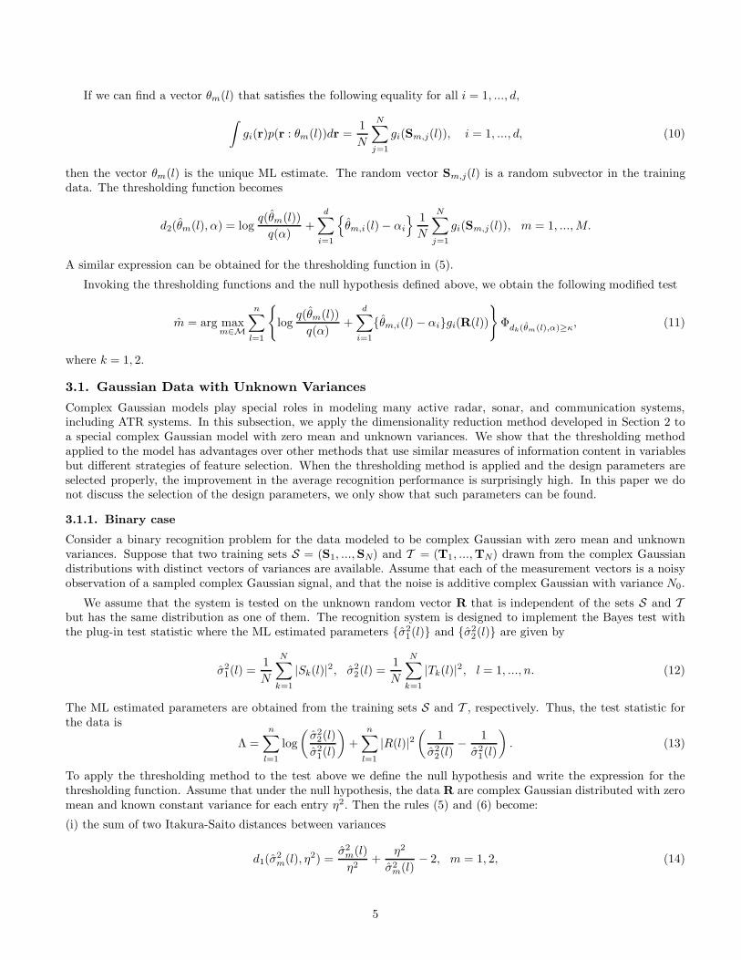
d1(θ̂m(l), ψ(l)) = D(θm(l) : ψ(l))|θ̂m(l) + D(ψ(l) : θm(l))|θ̂m(l) (5)

=

∫

p(r : θm(l)) logp(r : θm(l))

p(r : ψ(l))dr

∣

∣

∣

∣

θ̂m(l)

+

∫

p(r : ψ(l)) logp(r : ψ(l))

p(r : θm(l))dr

∣

∣

∣

∣

θ̂m(l)

,

or

d2(θ̂m(l), ψ(l)) = D(θm(l) : ψ(l))|θ̂m(l) =

∫

p(r : θm(l)) logp(r : θm(l))

p(r : ψ(l))dr

∣

∣

∣

∣

θ̂m(l)

. (6)

The function D(· : ·) is relative entropy.13

3

To incorporate the variable selection rule in the Bayes test we simply multiply each term of the sum in (3) by theindicator function of the distance given in (4). Thus, the modified test is given by

m̂ = arg maxm∈M

n∑

l=1

{

log{

p(R(l) : θ̂m(l))}

− log {p(R(l) : ψ(l))}}

Φdk(θ̂m(l),ψ(l))≥κ, (7)

where ΦE is the indicator function of the event E , and dk(·, ·), k = 1, 2, are given by (5) and (6), respectively.

Comment 2: The discriminating measures (i), (ii) involve the parameters of the null hypothesis. This makes thediscriminating measure more robust.

Comment 3: The number of variables selected using the rule (4) is random.

3. EXPONENTIAL FAMILY

Consider the exponential family of populations. The probability density function of a random h-dimensional vector Y

is given by

p(y : θ) = q(θ)r(y) exp

{

d∑

i=1

θigi(y)

}

,

where y is the row vector y = (y1, y2, ..., yh), θ is the row vector θ = (θ1, ..., θd), q(θ) and r(y) are nonnegative functionsof θ and y, respectively, and θ ∈ Θ ⊂ Rd, where Θ is an open convex set.

Consider now a random vector X obtained by combining n independent random subvectors X(l), l = 1, ..., n, eachof size h. The distribution of each subvector X(l) is parameterized by a d-dimensional vector of parameters θ(l). Thenthe probability density function for the random vector X can be written as

p(x : θ) =

n∏

l=1

p(x(l) : θ(l)) =

n∏

l=1

q(θ(l))r(x(l)) exp

{

d∑

i=1

θi(l)gi(x(l))

}

, (8)

where x is an hn-dimensional realization of vector X.

Consider a recognition problem with M ≥ 2 populations and data modeled to belong to the exponential familydefined above. Suppose that M training sets denoted as Sm, m ∈ M = {1, ...,M}, (one for each population) areavailable to estimate the unknown parameters of the probability density functions using the ML estimation procedure.As in Section 2, each training set consists of N independent and identically distributed realizations.

A simple Bayes test with the plug-in test statistics is used to classify the hn dimensional vector R

m̂ = arg maxm∈M

log{

p1(R : θ̂m)}

= arg maxm∈M

{

n∑

l=1

log{

q(θ̂m(l))}

+

n∑

l=1

d∑

i=1

θ̂m,i(l)gi(R(l))

}

, (9)

where θ̂m(l), m = 1, ...,M, is a d-dimensional vector of the parameters related to the l-th testing sub-vector andobtained using the set Sm. Recall that the testing data R can be distributed as one of the sets Sm but independent ofall the training sets.

To obtain the modified test, let us introduce a null hypothesis and the thresholding function. Suppose that underthe null hypothesis, the testing data R are exponentially distributed with a known d-dimensional vector of parametersα = (α1, ..., αd), where α is a design parameter. In this section, assume that under the null hypothesis each entry ofthe testing vector R is parameterized by the same vector α.

Consider the thresholding function in (6). For the exponential family we have

d2(θ̂m(l), α) = logq(θ̂m(l))

q(α)+

d∑

i=1

{

θ̂m,i(l) − αi

}

∫

gi(r)p(r : θm(l))dr

∣

∣

∣

∣

θm(l)=θ̂m(l)

, m = 1, ...,M,

where p(r : θm(l)) is the probability density function of the random vector R(l) under the hypothesis m.

4

If we can find a vector θm(l) that satisfies the following equality for all i = 1, ..., d,

∫

gi(r)p(r : θm(l))dr =1

N

N∑

j=1

gi(Sm,j(l)), i = 1, ..., d, (10)

then the vector θm(l) is the unique ML estimate. The random vector Sm,j(l) is a random subvector in the trainingdata. The thresholding function becomes

d2(θ̂m(l), α) = logq(θ̂m(l))

q(α)+

d∑

i=1

{

θ̂m,i(l) − αi

} 1

N

N∑

j=1

gi(Sm,j(l)), m = 1, ...,M.

A similar expression can be obtained for the thresholding function in (5).

Invoking the thresholding functions and the null hypothesis defined above, we obtain the following modified test

m̂ = arg maxm∈M

n∑

l=1

{

logq(θ̂m(l))

q(α)+

d∑

i=1

{θ̂m,i(l) − αi}gi(R(l))

}

Φdk(θ̂m(l),α)≥κ, (11)

where k = 1, 2.

3.1. Gaussian Data with Unknown Variances

Complex Gaussian models play special roles in modeling many active radar, sonar, and communication systems,including ATR systems. In this subsection, we apply the dimensionality reduction method developed in Section 2 toa special complex Gaussian model with zero mean and unknown variances. We show that the thresholding methodapplied to the model has advantages over other methods that use similar measures of information content in variablesbut different strategies of feature selection. When the thresholding method is applied and the design parameters areselected properly, the improvement in the average recognition performance is surprisingly high. In this paper we donot discuss the selection of the design parameters, we only show that such parameters can be found.

3.1.1. Binary case

Consider a binary recognition problem for the data modeled to be complex Gaussian with zero mean and unknownvariances. Suppose that two training sets S = (S1, ...,SN) and T = (T1, ...,TN) drawn from the complex Gaussiandistributions with distinct vectors of variances are available. Assume that each of the measurement vectors is a noisyobservation of a sampled complex Gaussian signal, and that the noise is additive complex Gaussian with variance N0.

We assume that the system is tested on the unknown random vector R that is independent of the sets S and Tbut has the same distribution as one of them. The recognition system is designed to implement the Bayes test withthe plug-in test statistic where the ML estimated parameters {σ̂2

1(l)} and {σ̂22(l)} are given by

σ̂21(l) =

1

N

N∑

k=1

|Sk(l)|2, σ̂2

2(l) =1

N

N∑

k=1

|Tk(l)|2, l = 1, ..., n. (12)

The ML estimated parameters are obtained from the training sets S and T , respectively. Thus, the test statistic forthe data is

Λ =

n∑

l=1

log

(

σ̂22(l)

σ̂21(l)

)

+

n∑

l=1

|R(l)|2(

1

σ̂22(l)

−1

σ̂21(l)

)

. (13)

To apply the thresholding method to the test above we define the null hypothesis and write the expression for thethresholding function. Assume that under the null hypothesis, the data R are complex Gaussian distributed with zeromean and known constant variance for each entry η2. Then the rules (5) and (6) become:

(i) the sum of two Itakura-Saito distances between variances

d1(σ̂2m(l), η2) =

σ̂2m(l)

η2+

η2

σ̂2m(l)

− 2, m = 1, 2, (14)

5

0 50 100 1500

2

4

6

8

10

RANGE BINSV

AR

IAN

CE

, (m

4 )0 50 100 150

0

10

20

30

40

50

RANGE BINS

VA

RIA

NC

E, (

m4 )

0 50 100 1500

2

4

6

8

10

12

14

RANGE BINS

VA

RIA

NC

E, (

m4 )

0 50 100 1500

10

20

30

40

50

60

70

RANGE BINS

VA

RIA

NC

E, (

m4 )

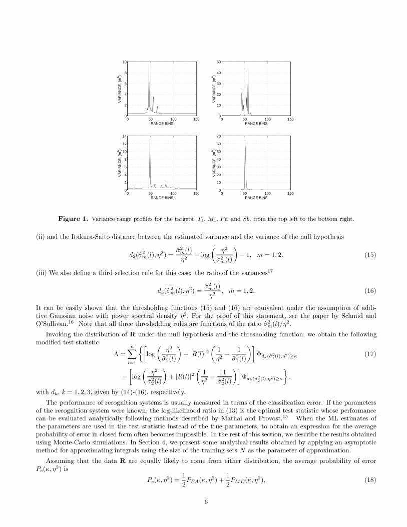
Figure 1. Variance range profiles for the targets: T1, M1, F t, and Sb, from the top left to the bottom right.

(ii) and the Itakura-Saito distance between the estimated variance and the variance of the null hypothesis

d2(σ̂2m(l), η2) =

σ̂2m(l)

η2+ log

(

η2

σ̂2m(l)

)

− 1, m = 1, 2. (15)

(iii) We also define a third selection rule for this case: the ratio of the variances17

d3(σ̂2m(l), η2) =

σ̂2m(l)

η2, m = 1, 2. (16)

It can be easily shown that the thresholding functions (15) and (16) are equivalent under the assumption of addi-tive Gaussian noise with power spectral density η2. For the proof of this statement, see the paper by Schmid andO’Sullivan.16 Note that all three thresholding rules are functions of the ratio σ̂2

m(l)/η2.

Invoking the distribution of R under the null hypothesis and the thresholding function, we obtain the followingmodified test statistic

Λ̃ =

n∑

l=1

{[

log

(

η2

σ̂21(l)

)

+ |R(l)|2(

1

η2−

1

σ̂21(l)

)]

Φdk(σ̂2

1(l),η2)≥κ (17)

−

[

log

(

η2

σ̂22(l)

)

+ |R(l)|2(

1

η2−

1

σ̂22(l)

)]

Φdk(σ̂2

2(l),η2)≥κ

}

,

with dk, k = 1, 2, 3, given by (14)-(16), respectively.

The performance of recognition systems is usually measured in terms of the classification error. If the parametersof the recognition system were known, the log-likelihood ratio in (13) is the optimal test statistic whose performancecan be evaluated analytically following methods described by Mathai and Provost.15 When the ML estimates ofthe parameters are used in the test statistic instead of the true parameters, to obtain an expression for the averageprobability of error in closed form often becomes impossible. In the rest of this section, we describe the results obtainedusing Monte-Carlo simulations. In Section 4, we present some analytical results obtained by applying an asymptoticmethod for approximating integrals using the size of the training sets N as the parameter of approximation.

Assuming that the data R are equally likely to come from either distribution, the average probability of errorPe(κ, η

2) is

Pe(κ, η2) =

1

2PFA(κ, η2) +

1

2PMD(κ, η2), (18)

6

0 10 20 30 40 500.06

0.08

0.1

0.12

0.14

0.16

0.18

0.2

SEGMENTATION LEVEL

PR

OB

AB

ILIT

Y O

F E

RR

OR

0 10 20 30 40 500.05

0.1

0.15

0.2

0.25

SEGMENTATION LEVEL

PR

OB

AB

ILIT

Y O

F E

RR

OR

0 10 20 30 40 500

0.05

0.1

0.15

0.2

SEGMENTATION LEVEL

PR

OB

AB

ILIT

Y O

F E

RR

OR

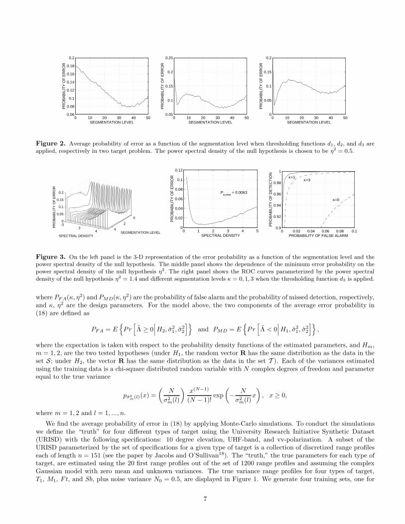
Figure 2. Average probability of error as a function of the segmentation level when thresholding functions d1, d2, and d3 areapplied, respectively in two target problem. The power spectral density of the null hypothesis is chosen to be η2 = 0.5.

0

2

40

24

0

0.05

0.1

0.15

0.2

SEGMENTATION LEVELSPECTRAL DENSITY

PR

OB

AB

ILIT

Y O

F E

RR

OR

0 1 2 3 4 50

0.02

0.04

0.06

0.08

0.1

0.12

SPECTRAL DENSITY

PR

OB

AB

ILIT

Y O

F E

RR

OR

Pe,min

= 0.0063

0 0.02 0.04 0.06 0.08 0.10.9

0.92

0.94

0.96

0.98

1

PROBABILITY OF FALSE ALARM

PR

OB

AB

ILIT

Y O

F D

ET

EC

TIO

N

κ=0

κ=3κ=1

Figure 3. On the left panel is the 3-D representation of the error probability as a function of the segmentation level and thepower spectral density of the null hypothesis. The middle panel shows the dependence of the minimum error probability on thepower spectral density of the null hypothesis η2. The right panel shows the ROC curves parameterized by the power spectraldensity of the null hypothesis η2 = 1.4 and different segmentation levels κ = 0, 1, 3 when the thresholding function d3 is applied.

where PFA(κ, η2) and PMD(κ, η2) are the probability of false alarm and the probability of missed detection, respectively,and κ, η2 are the design parameters. For the model above, the two components of the average error probability in(18) are defined as

PFA = E{

Pr[

Λ̃ ≥ 0∣

∣

∣H2, σ̂21, σ̂

22

]}

and PMD = E{

Pr[

Λ̃ < 0∣

∣

∣H1, σ̂21 , σ̂

22

]}

,

where the expectation is taken with respect to the probability density functions of the estimated parameters, and Hm,m = 1, 2, are the two tested hypotheses (under H1, the random vector R has the same distribution as the data in theset S; under H2, the vector R has the same distribution as the data in the set T ). Each of the variances estimatedusing the training data is a chi-square distributed random variable with N complex degrees of freedom and parameterequal to the true variance

pσ̂2m

(l)(x) =

(

N

σ2m(l)

)

x(N−1)

(N − 1)!exp

(

−N

σ2m(l)

x

)

, x ≥ 0,

where m = 1, 2 and l = 1, ..., n.

We find the average probability of error in (18) by applying Monte-Carlo simulations. To conduct the simulationswe define the “truth” for four different types of target using the University Research Initiative Synthetic Dataset(URISD) with the following specifications: 10 degree elevation, UHF-band, and vv-polarization. A subset of theURISD parameterized by the set of specifications for a given type of target is a collection of discretized range profileseach of length n = 151 (see the paper by Jacobs and O’Sullivan18). The “truth,” the true parameters for each type oftarget, are estimated using the 20 first range profiles out of the set of 1200 range profiles and assuming the complexGaussian model with zero mean and unknown variances. The true variance range profiles for four types of target,T1, M1, F t, and Sb, plus noise variance N0 = 0.5, are displayed in Figure 1. We generate four training sets, one for

7

Pe T1 −M1 T1 − F t T1 − Sb M1 − F t M1 − Sb F t− Sb

Full Dimension 0.1764 0.2337 0.1089 0.0747 0.0117 0.1341Reduced Dimension 0.0063 0.0527 0.0011 0.0003 < 10−4 0.0024

κ 1 0.8 1.4 1 1.2 1.6

η2 1.4 1.2 1.8 1.4 1 1

Figure 4. The table presents a summary of a pairwise performance comparison for four targets. There are four rows thatdescribe each pair of targets. In the first row, we place the results of simulation with the segmentation level set to be zero (noreduction dimensionality method is applied). The entries of the second row are obtained by finding the minimum of the errorprobability over all values κ and η2. The fourth and the fifth rows contain the parameters that result in the smallest value ofthe error probability.

each type of target, and each of size N = 3. The testing data are generated independently of the training sets. Theprobability of error is computed by generating independent realizations of the modified log-likelihood ratio in (17). InFigure 2, we present simulation results for the pair T1 −M1. Three panels (left to right) show the dependence of theaverage probability of error on the segmentation level κ when three different thresholding functions are applied d1, d2,and d3, respectively. The variance of the null hypothesis η2 and the variance of the white complex Gaussian noise N0

are selected to be equal, η2 = N0 = 0.5, in this example. All three cases show the presence of the peaking phenomenon.Note a complex behavior of the error probability when the thresholding functions d2 and d3 are used. The best resultis achieved by applying the thresholding function d3. The plots in Figure 3 were generated for the pair of targets T1 -M1. On the left panel in Figure 3, we show a three-dimensional plot of the error probability as a function of the twoparameters κ and η2. The global minimum of the probability of error is achieved at the point (1, 1.4) and is equal to0.0063. The plot on the middle panel is obtained as follows. For each given value of the variance η2 we compute theminimum of the error probability over the segmentation level and then plot this value versus the value of the spectraldensity η2. The ROC curves parameterized by three values of the segmentation level κ = 0, 1, 3 and the power spectraldensity η2 = 1.4 are shown on the right panel. Note that the test statistic in (17) with κ = 0 is equivalent to the teststatistic in (13). In the table in Figure 4, we give a summary of the results for six pairs of targets. The third row ofthe table shows the probability of error that can be achieved when the test in (17) is implemented. In the fourth andthe fifth rows of the table we specify the parameters κ and η2 that result in the smallest value of the error probability.

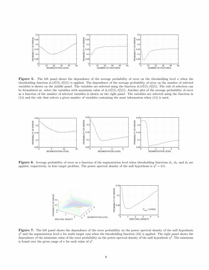
For comparison, we present results obtained by applying three modifications of the algorithm described in Section2. These algorithms use thresholding functions of the same form as (14) to select the individual components but differeither in the feature selection rule, or in how variables are plugged in the thresholding function. All simulation resultspresented in Figure 5 were obtained for the pair T1 −M1. On the left panel in Figure 5, the dependence of the averageprobability of error on the thresholding level is shown for the case when variables in the measurement vectors areselected using the following thresholding function d1(σ̂

21(l), σ̂

22(l)) = σ̂2

1(l)/σ̂22(l) + σ̂2

2(l)/σ̂21(l) − 2. The distribution

of the null hypothesis is excluded from the test statistic. This results in a less robust estimate of the thresholdingfunction and hence in degradation of performance. The middle panel shows the plot of the average probability of erroras a function of the number of selected variables. The variables are selected using the same thresholding functiond1(σ̂

21(l), σ̂

22(l)) as above, but a different rule for selecting the best features. In this case, a fixed number of features

corresponding to the largest values of the function d1(σ̂21(l), σ̂

22(l)) are selected. On the right panel, we plot the average

probability of error as a function of the number of selected variables. The variables are selected using the thresholdingfunction in (14) with η2 = 0.2, but the selection rule selects a fixed number of features corresponding to the largestvalues of the function in (14). The results show the advantage of introducing a null hypothesis that results in morerobust estimates of the thresholding function.

3.1.2. M-ary case

In this subsection, we analyze the performance for the M -ary case, with M = 4. The variance range profiles that weuse as a “truth” are shown in Figure 1. The test for the complex Gaussian model is given by

m̂ = arg maxm∈M

n∑

l=1

{

|Rl|2

(

1

η2−

1

σ̂2m(l)

)

+ log

(

η2

σ̂2m(l)

)}

Φdk(σ̂2m

(l),η2)≥κ, (19)

where the thresholding functions dk, k = 1, 2, 3, are given by (14), (15), and (16), respectively.

8

0 10 20 30 40 500

0.05

0.1

0.15

0.2

0.25

0.3

SEGMENTATION LEVEL

PR

OB

AB

ILIT

Y O

F E

RR

OR

0 10 20 30 40 500

0.05

0.1

0.15

0.2

0.25

0.3

NUMBER OF FEATURES

PR

OB

AB

ILIT

Y O

F E

RR

OR

0 10 20 30 40 500

0.05

0.1

0.15

0.2

0.25

0.3

NUMBER OF FEATURES

PR

OB

AB

ILIT

Y O

F E

RR

OR

Figure 5. The left panel shows the dependence of the average probability of error on the thresholding level κ when thethresholding function d1(σ̂

2

1(l), σ̂2

2(l)) is applied. The dependence of the average probability of error on the number of selectedvariables is shown on the middle panel. The variables are selected using the function d1(σ̂

2

1(l), σ̂2

2(l)). The rule of selection canbe formulated as: select the variables with maximum value of d1(σ̂

2

1(l), σ̂2

2(l)). Another plot of the average probability of erroras a function of the number of selected variables is shown on the right panel. The variables are selected using the function in(14) and the rule that selects a given number of variables containing the most information when (14) is used.

0 5 10 150.05

0.1

0.15

0.2

0.25

SEGMENTATION LEVEL

PR

OB

AB

ILIT

Y O

F E

RR

OR

0 2 4 60.05

0.1

0.15

0.2

0.25

SEGMENTATION LEVEL

PR

OB

AB

ILIT

Y O

F E

RR

OR

0 1 2 3 4 50.05

0.1

0.15

0.2

0.25

SEGMENTATION LEVEL

PR

OB

AB

ILIT

Y O

F E

RR

OR

Figure 6. Average probability of error as a function of the segmentation level when thresholding functions d1, d2, and d3 areapplied, respectively, in four target problem. The power spectral density of the null hypothesis is η2 = 0.5.

01

23

45

02

4

0

0.2

0.4

SEGMENTATION LEVELSPECTRAL DENSITY

PR

OB

AB

ILIT

Y O

F E

RR

OR

0 1 2 3 4 50

0.05

0.1

0.15

SPECTRAL DENSITY

PR

OB

AB

ILIT

Y O

F E

RR

OR

Pmin

= 0.0324

Figure 7. The left panel shows the dependence of the error probability on the power spectral density of the null hypothesisη2 and the segmentation level κ for multi target case when the thresholding function (16) is applied. The right panel shows thedependence of the minimum value of the error probability on the power spectral density of the null hypothesis η2. The minimumis found over the given range of κ for each value of η2.

9

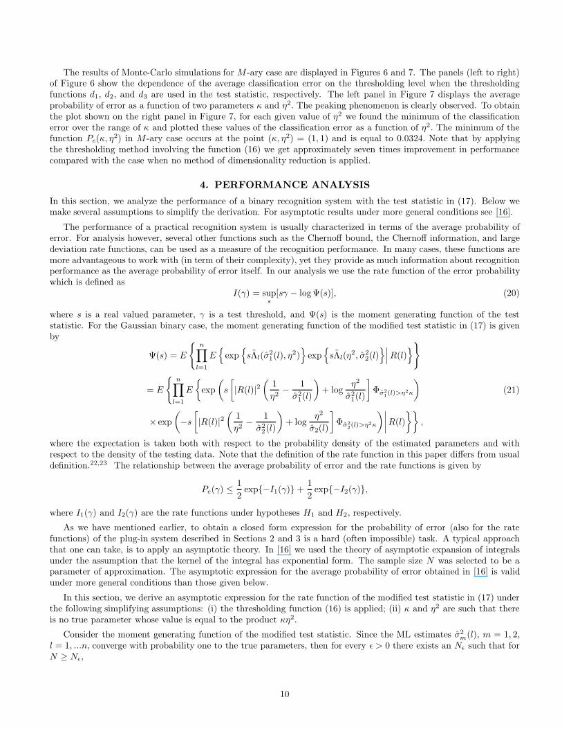
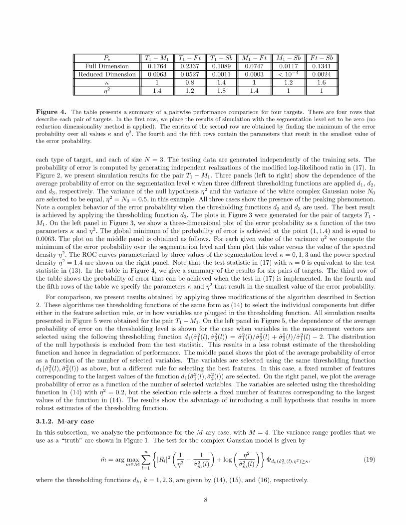
The results of Monte-Carlo simulations for M -ary case are displayed in Figures 6 and 7. The panels (left to right)of Figure 6 show the dependence of the average classification error on the thresholding level when the thresholdingfunctions d1, d2, and d3 are used in the test statistic, respectively. The left panel in Figure 7 displays the averageprobability of error as a function of two parameters κ and η2. The peaking phenomenon is clearly observed. To obtainthe plot shown on the right panel in Figure 7, for each given value of η2 we found the minimum of the classificationerror over the range of κ and plotted these values of the classification error as a function of η2. The minimum of thefunction Pe(κ, η

2) in M -ary case occurs at the point (κ, η2) = (1, 1) and is equal to 0.0324. Note that by applyingthe thresholding method involving the function (16) we get approximately seven times improvement in performancecompared with the case when no method of dimensionality reduction is applied.

4. PERFORMANCE ANALYSIS

In this section, we analyze the performance of a binary recognition system with the test statistic in (17). Below wemake several assumptions to simplify the derivation. For asymptotic results under more general conditions see [16].

The performance of a practical recognition system is usually characterized in terms of the average probability oferror. For analysis however, several other functions such as the Chernoff bound, the Chernoff information, and largedeviation rate functions, can be used as a measure of the recognition performance. In many cases, these functions aremore advantageous to work with (in term of their complexity), yet they provide as much information about recognitionperformance as the average probability of error itself. In our analysis we use the rate function of the error probabilitywhich is defined as

I(γ) = sups

[sγ − logΨ(s)], (20)

where s is a real valued parameter, γ is a test threshold, and Ψ(s) is the moment generating function of the teststatistic. For the Gaussian binary case, the moment generating function of the modified test statistic in (17) is givenby

Ψ(s) = E

{

n∏

l=1

E{

exp{

sΛ̃l(σ̂21(l), η

2)}

exp{

sΛ̃l(η2, σ̂2

2(l)}∣

∣

∣R(l)}

}

= E

{

n∏

l=1

E

{

exp

(

s

[

|R(l)|2(

1

η2−

1

σ̂21(l)

)

+ logη2

σ̂21(l)

]

Φσ̂2

1(l)>η2κ

)

(21)

× exp

(

−s

[

|R(l)|2(

1

η2−

1

σ̂22(l)

)

+ logη2

σ̂2(l)

]

Φσ̂2

2(l)>η2κ

)∣

∣

∣

∣

R(l)

}}

,

where the expectation is taken both with respect to the probability density of the estimated parameters and withrespect to the density of the testing data. Note that the definition of the rate function in this paper differs from usualdefinition.22,23 The relationship between the average probability of error and the rate functions is given by

Pe(γ) ≤1

2exp{−I1(γ)} +

1

2exp{−I2(γ)},

where I1(γ) and I2(γ) are the rate functions under hypotheses H1 and H2, respectively.

As we have mentioned earlier, to obtain a closed form expression for the probability of error (also for the ratefunctions) of the plug-in system described in Sections 2 and 3 is a hard (often impossible) task. A typical approachthat one can take, is to apply an asymptotic theory. In [16] we used the theory of asymptotic expansion of integralsunder the assumption that the kernel of the integral has exponential form. The sample size N was selected to be aparameter of approximation. The asymptotic expression for the average probability of error obtained in [16] is validunder more general conditions than those given below.

In this section, we derive an asymptotic expression for the rate function of the modified test statistic in (17) underthe following simplifying assumptions: (i) the thresholding function (16) is applied; (ii) κ and η2 are such that thereis no true parameter whose value is equal to the product κη2.

Consider the moment generating function of the modified test statistic. Since the ML estimates σ̂2m(l), m = 1, 2,

l = 1, ...n, converge with probability one to the true parameters, then for every ǫ > 0 there exists an Nǫ such that forN ≥ Nǫ,

10

−10 −5 0 5 100

2

4

6

8

10

T, PARAMETER

RA

TE

FU

NC

TIO

N

I1

I2

Figure 8. Three pairs of the rate functions are shown in this figure: the “dashed-dotted” lines correspond to the ideal ratefunctions; the “dashed” lines correspond to the rate functions for the test with the test statistic in (13); and the “solid” linescorrespond to the rate functions for the test with the test statistic in (17). The parameters used are N = 30, η2 = 0.6, andκ = 1.

Ψ(s|R) =

n∏

l=1

E

exp{

sΛ̃l(σ21(l), η

2)}

1 +

1

2(σ̂2

1(l) − σ21(l))

2

∂2Λ̃(l)

(∂σ̂21(l))2

+

[

∂Λ̃(l)

∂σ̂21(l)

]2

∣

∣

∣

∣

∣

∣

σ2

1,σ2

2

+ o(

(σ̂21(l) − σ2

1(l))2)

(22)

× exp{

sΛ̃l(η2, σ2

2(l))}

1 +

1

2(σ̂2

2(l) − σ22(l))

2

∂2Λ̃(l)

(∂σ̂22(l))

2+

[

∂Λ̃(l)

∂σ̂22(l)

]2

∣

∣

∣

∣

∣

∣

σ2

1,σ2

2

+ o(

(σ̂22(l) − σ2

2(l))2)

∣

∣

∣

∣

∣

∣

∣

R(l)

.

The rest of the derivation follows the procedure in [19]. The expectation in (22) in many cases can be found in closedform. Note if σ2

m(l) < κη2, the contribution of the integral is equal to one. If σ2m(l) > κη2, the contribution of the

integral can be found from (22). After the expectation in (22) is taken, we plug this expression into (20).

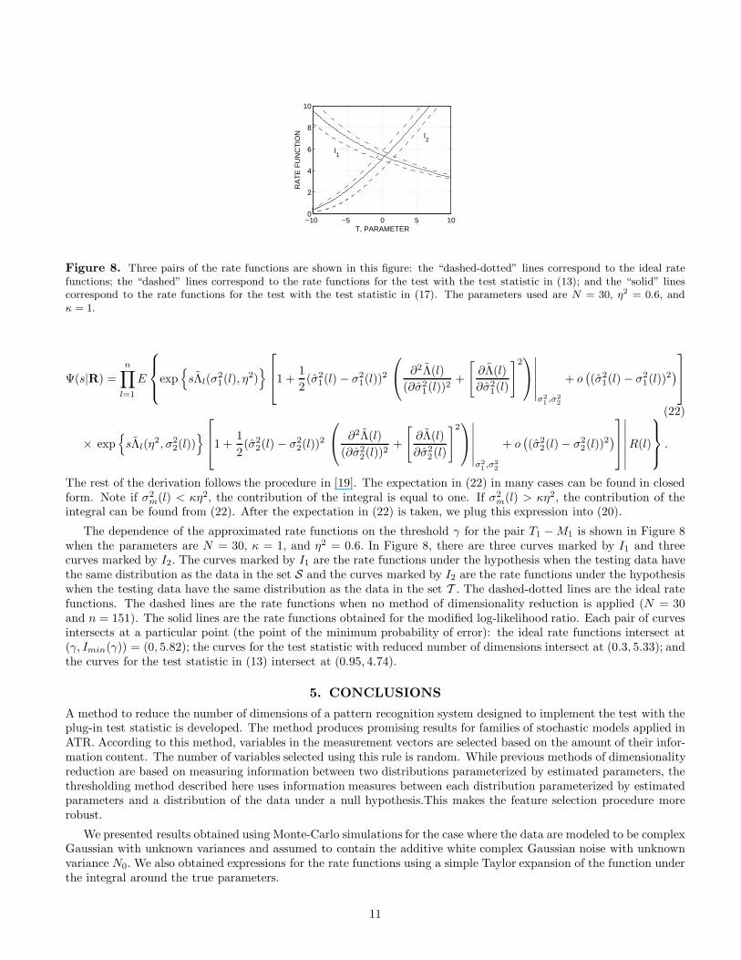
The dependence of the approximated rate functions on the threshold γ for the pair T1 −M1 is shown in Figure 8when the parameters are N = 30, κ = 1, and η2 = 0.6. In Figure 8, there are three curves marked by I1 and threecurves marked by I2. The curves marked by I1 are the rate functions under the hypothesis when the testing data havethe same distribution as the data in the set S and the curves marked by I2 are the rate functions under the hypothesiswhen the testing data have the same distribution as the data in the set T . The dashed-dotted lines are the ideal ratefunctions. The dashed lines are the rate functions when no method of dimensionality reduction is applied (N = 30and n = 151). The solid lines are the rate functions obtained for the modified log-likelihood ratio. Each pair of curvesintersects at a particular point (the point of the minimum probability of error): the ideal rate functions intersect at(γ, Imin(γ)) = (0, 5.82); the curves for the test statistic with reduced number of dimensions intersect at (0.3, 5.33); andthe curves for the test statistic in (13) intersect at (0.95, 4.74).

5. CONCLUSIONS

A method to reduce the number of dimensions of a pattern recognition system designed to implement the test with theplug-in test statistic is developed. The method produces promising results for families of stochastic models applied inATR. According to this method, variables in the measurement vectors are selected based on the amount of their infor-mation content. The number of variables selected using this rule is random. While previous methods of dimensionalityreduction are based on measuring information between two distributions parameterized by estimated parameters, thethresholding method described here uses information measures between each distribution parameterized by estimatedparameters and a distribution of the data under a null hypothesis.This makes the feature selection procedure morerobust.

We presented results obtained using Monte-Carlo simulations for the case where the data are modeled to be complexGaussian with unknown variances and assumed to contain the additive white complex Gaussian noise with unknownvariance N0. We also obtained expressions for the rate functions using a simple Taylor expansion of the function underthe integral around the true parameters.

11

O’Sullivan and DeVore20,21 have performed a systematic study of ATR performance versus the complexity of datamodels. The study has used the public-domain MSTAR database. These real data have actual targets in clutter, inaddition to any sensor noise. In order to apply the methods in this paper to the MSTAR data, the null hypothesismust be extended to model both the clutter and any sensor noise.

6. ACKNOWLEDGMENTS

This work was supported in part by the US Army Research Office grant DAAH04-95-1-0494, by the Office of NavalResearch grant N00014-98-1-06-06, and by the Boeing McDonnell Foundation.

REFERENCES

1. A. K. Jain, R. P. W. Duin, and J. Mao, “Statistical Pattern Recognition: A Review,” IEEE Trans. on Pattern Analysis

and Machine Intelligence, v. 22, no. 1, pp. 4-36, January 2000.

2. L. Devroye, L. Gyorfi, and G. Lugosi, A Probabilistic Theory of Pattern Recognition, Springer, New York, 1996.

3. R. O. Duda and P. E. Hart, Pattern Classification and Scene Analysis, John Wiley & Sons, New York, 1983

4. G. V. Trunk, “A Problem of Dimensionality: A Simple Example,” IEEE Trans. on Pattern Analysis and Machine Intelli-

gence, vol. 1, no. 3, July 1979, pp. 306-307.

5. S. J. Raudys and A. K. Jain, “Small Sample Size Effects in Statistical Pattern Recognition: Recommendations for Practi-tioners,” IEEE Trans. on Pattern Analysis and Machine Intelligence, vol. 13, no. 3, March 1991, pp. 252-264.

6. A. K. Jain and B. Chandrasekaran, “Dimensionality and Sample Size Considerations in Pattern Recognition Practice,”Handbook in Statistic, Vol. 2, ( P. R. Krishnaiah and L. N. Kanal, eds.), North-Holland Publishing Company, 1982, pp.835-855.

7. L. Kanal, B. Chandrasekaran, “On Dimensionality and Sample Size in Statistical Pattern Classification,” Pattern Recog-

nition, vol.3, 1971, pp. 225-234.

8. M. Ben-Bassat, “Use of Distance Measures, Information Measures and Error Bounds in Feature Evaluation,” in Handbook

of Statistics, vol. 2, ( P. R. Krishnaiah and L. N. Kanal, eds.), North-Holland Publishing Company, 1982, pp. 773-791.

9. W. Siedlecki and J. Sklansky, “A Note on Genetic Algorithm for Large-Scale Feature Selection,” Pattern Recognition Lett.,vol. 10, 1989, pp. 335-347.

10. A. Jain and D. Zongker, “Feature Selection: Evaluation, Application, and Small Sample Performance,” IEEE Trans.

Pattern Analysis and Machine Intelligence, vol. 19, no. 2, Feb. 1997, pp. 153-158.

11. P. M. Narendra and K. Fukunaga, “A Branch and Bound Algorithm for Feature Subset Selection,” IEEE Trans. Computers,vol. 26, no. 9, Sept. 1977, pp. 917-922.

12. P. Pudil, J. Novovicova, and J. Kittler, “Floating Search Methods in Feature Selection,” Pattern Recognition Letters, vol.15, 1994, pp. 1,119-1,125.

13. S. Kullback, Information Theory and Statistics, Dover Publications, Inc., 1997.

14. N. Bleistein and R. A. Handelsman, Asymptotic Expansions of Integrals, Dover Publications Inc., Mineola, New York, 1986,pp. 187-199.

15. A. M. Mathai and S. B. Provost, Quadratic Forms in Random Variables, Marcel Dekker, Inc., New York, 1992, pp. 135-141.

16. N. A. Schmid, J. A. O’Sullivan, “Thresholding Method for Reduction of Dimensionality,” submitted to IEEE Trans. onInfo. Theory.

17. L. L. Horowitz and G. F. Brendel, “Fundamental SAR ATR Performance Predictions for Design Tradeoffs,” in SPIE Proc.

Algorithms for Synthetic Aperture Radar Imagery IV, vol. 3070, Orlando, FL, 23-24 April, 1997, pp. 267-284.

18. S. P. Jacobs and J. A. O’Sullivan, “Automatic Target Recognition Using Sequences of High Resolution Radar Range-Profiles,” IEEE Transactions on Aerospace and Electronic Systems, to appear 2000.

19. K. Fukunaga, R. R. Hayes, “Effect of Sample Size in Classifier Design,” IEEE Trans. Pattern Analysis and Machine

Intelligence, vol. 11, no. 8, Aug. 1989, pp. 873-885.

20. Joseph A. O’Sullivan and Michael D. DeVore, “Performance-Complexity Tradeoffs for Several Approaches to ATR fromSAR Images,” Proceedings of SPIE 2000, to be published.

21. Michael D. DeVore, Aaron D. Lanterman, Joseph A. O’Sullivan, “ATR Performance of a Rician Model for SAR Images,”Proceedings of SPIE 2000, to be published.

22. H. L. Van Trees, Detection, Estimation, and Modulation Theory, Wiley & Sons, Inc., New York, 1968.

23. J. A. Bucklew, Large Deviation Techniques in Decision, Simulation, and Estimation, John Willey & Sons, Inc., 1990.

12