ELSEVIER Journal of Econometrics 77 (1997) 8 7 103

JOURNAL OF Econometrics

Socioeconomic inequalities in health: Measurement, computation, and statistical inference

Nanak Kakwani *'a, Adam Wagstaff b, Eddy van Doorslaeff

"~ School of Economics, University of New South Wales, Sydney, NSW 2052. Australia School of Social Sciences. Unit~ersi O, of Sussex, Brighton BNI 9QN, UK

Department o/" Health Policy and Management, Erasmus UniversiO,. 3000 DR Rotterdam. The Netherlands

Abstract

This paper clarifies the relationship between two widely used indices of health inequal- ity and explains why these are superior to others indices used in the literature. It also develops asymptotic estimators for their variances and clarifies the role that demographic standardization plays in the analysis of socioeconomic inequalities in health. Empirical illustrations are presented for Dutch health survey data.

Key u'ords: Socioeconomic ;nequality; Concentration index; Standard errors JEL chtssilication: 1112

I. Introduction

This paper clarifies the relationship between two widely used indices of health inequality, namely the relative index of inequality (Rll) and the concentration index (CI). it explains why these are superior to other indices used in the empirical literature. The paper also clarifies the role that demographic standard- ization plays in the analysis of socioeconomic inequities in health.

Since the indices of health inequality are generally estimated from sample observations, it is useful to be able to test whether any observed differences in

* Corresponding author.

This paper derives from tile project "Equity in the finance and delivery of health care in Eutope'. which is funded by the European Community's Biomet Programme (contract BMH1-CI'92-608). We are grateful to the EC for financial support. We are also grateful to Hart Bliechrodt for his help in the research leading up to this paper and for him, Alok Bhargava and three referees for helpful comments on a previous draft. We alone are responsible for any errors.

0304-4076/97/$15.00 tl, 1997 Elsevier Science S.A. All rights reserved Pil S 0 3 0 4 - 4 0 7 6 ( 9 6 J 0 1 8~7 - 6

88 N. Kalavani et al. / Journal q f Economea'ics 77 (1997) 87-103

their values are statistically significant. This paper develops accurate distribu- tion-free asymptotic estimators of the standard errors of both the R|I and CI. There is, of course, an extensive literature on the sampling properties of the Gini index to which the CI is related (Nygord and Sanst/Sm, 1981; Kakwani, 1990; Cowell, 1989). These sampling distributions are derived by applying Hoeffding's (1948) theorem on order statistics. This methodology cannot be applied to derive the sampling distribution of CIs because they can be both negative and positive and, therefore, cannot be written in the form of order statistics. Thus, the derivations of the standard error fo,'mulae of this paper (presented in the Appendix) are new, providing more general results. The formulae in the current paper reduce to the standard formulae for the Gini index when ranking by ill-health coincides with socioeconomic ranking (see Appendix B).

2. Two indices o f soc ioeconomic inequali ty in health

The illness concentration curve plots the cumulative proportion of the popu- lation - ranked by socioeconomic status (SES), beginning with the least advan- taged - against the cumulative proportion of illness.t If L(s) lies above (below) the diagonal, inequalities in illness favour the more (less} advantaged members of society. Health inequality can he measured by the CI, denoted below by C, defined as twice the area between L(st and the diagonal:

I

C = I ~ 2,!' L(s) ds. ( I ) o

C takes a value of zero when L(s) coincides with the diagonal and is negative (positivci when L(s)lies above (below) the diagonal. 2

On individual-level data C can be computed straightforwardly. Let xi (i = 1 . . . . . n) be the ill-health score of the ith individual. Each of the n indi- viduals arc then ranked according to their SES, beginning with the most disadvantaged. C can then be calculated as

C = ~ xiRi - l, (2) i = l

Cf. Wagstaffct al. (19891. On concentration curves and indices more generally, see Kakwani l! 977, 1980) and Lambert {19931.

-' The minimum and maximum values of C using individual-level data are - I and + I respectively: these occur when all the population's ill-health is concentrated in the hands of the most disadvan- tages person and tile least disadvantages person respectively.

N. Ka~vani et aL / Jol~rnal of Econometrics 77 (1997) 87-103 89

where ~u = (l/n)~]'= tx~ is the mean level of ill-health and R, is the relative rank of the ith person. Eq. (2) nmkea clear the dependence of C on the socioeconomic dimension to the distribution of ill-health. Suppose that person i's ill-health falls by an amount A, whilst person j's rises by the same amount. The effect on C is given by

2 A C = - - A ( R ~ - R j ) ,

which is clearly positive (negative) if i is more (less) disadvantaged than j. This sensitivity to the socioeconomic dimension to inequalities in health is not a feature of several other indices used in the literature. 3 Eq. (2) also makes clear that C depends on the ill-health of al l members of society.

Inequalities in health are frequently investigated using grouped data, the groups comprising socioeconomic groups (SEGs), social classes, groups of persons with similar levels of educational attainment, or income groups. 4 Let It, (t = 1, . . . , T) be the morbidity rate of the tth SEG and f, its population share. Rank the T SEGs according to their SES, beginning with the most disadvan- taged. If L ( s ) is assumed to be piecewZ,, linear, C can be calculated as

= - , ~ / I ~ R , - I, (3)

~ir_ ~ .fdt, being the mean morbidity rate, and R, is the relative rank of the tth SEG, defined as

R, = Y' £ + (4) ~'-I

and indicating the cumulative proportion of the population up to the midpoint of each group interval:

3 It is not true of the Gini coefficient (cf., e.g., lllsley and Le Grand, 19861, tile index of dissimilarity {cf., e.g., Preston et al., 1981), or the index of inequality {cf. Pappas et al., 1993). On this point cf. Wagstaff et al. (1991).

'* In cross-country comparisons in particular, the scope for meaningfull comparison is often limited by difference in the way groups arc defined. Some researchers have succeeded, however, in aclneving a higher degree of comparability with existing surveys {see, e.g., Vager6 and Lundberg, 1989: Kunst and Mackenbach, 1994). In any case tile problem is likely to become smaller over time, since various international organisations have launched initiatives aimed at harmonizing survey questions rel- evant to this area of research.

~ Eq. (3) makes clear the fact that, where grouped dam are used, C depends on the relative sizes of the SFGs, a property not shared by the range.

9 0 N. Kakwani et aL / Journal of Econometrics 77 (1997) 87-103

The Rll, which has invariably been used in the context of grouped data, is the slope of a regression of a group's relative morbidity, 14/#, on its relative rank, R,. The grouped nature of the data calls for Weighted Least Squares (WLS), the WLS estimate of the RII being easily obtained by running OLS on

= + R ,J , + .,, (5)

the estimator of/~, of which is equal to the RII. The RII and the CI are, in fact, related to one another by (cf. Wagstaff et al., 1991)

fl = C/2a~, (6) where a~ = E:'=, fAR, - ½).

3. Demographic factors and avoidable inequality

So far we have said nothing about the role demographic factors in generating health inequality - illness rates have been assumed to be crude illness rates. Comparing Lis) with the diagonal, or the RII with zero, presupposes that all socioeconomic inequalities in illness are avoidable. This is unrealistic, since there are biological influences on health that are to a large degree unalterable. It is clearly unreasonable, for example, to suppose that a person of 85 could be made as healthy as a 20-year old. The diagonal is thus an unsuitable benchmark against which to compare L(s) and zero is an unsuit0ble benchmark against which to compare the RII if crude morbidity rates are used in its calculation.

One approach is to use the direct method of standardization. This requires that grouped data be used and involves applying the age~ sex-specil~c average illness rates of each SEG to the age and gender structure of the population (cf., e.g., Rothman, 1986)]. The standardized ilhiess rate for SEG I is equal to

l e t - ~.. . ,~le,,,/ . . (7) d

where n,~ is the number of persons in the dth demographic group in the population as a whole. #,!t is the morbidity rate amongst persons in the dth demographic group in SEG t. If age-sex-specific morbidity rates are equal to the population rates in each age-sex group (i.e., itat= Ira Vd), the standardized rates will not vary across SEGs (i.e., it + = It Vt). The extent of avoidable inequality could be assessed by means of the RIi with the directly standardized rates (i.e., the lh ÷ ) being used instead of the unstandardized rates (i.e., the t4). Alternatively a directly standardized concentration curve can be constructed, denoted by L + (s), based on the each of the T SEGs" shares of standardized illness:

s: --.I; E ,,,,.,,, /E ,,,,.,,: (8) d / d

N. Ka&avani et al. / Journal of Econometrics 77 (1997) 87-103 91

these are equal to fr if/flat =/Ud 'v'd. If L ÷ (s) lies above the diagonal, the less advantages SEGs experience higher age-sex-specific illness rates than the popu- lation as a whole, whilst the opposite is true if L ÷ is) lies below the diagonal. Thus an alternative measure of avoidable inequalities in health is thus twice the area between L ÷ (s)and the diagonal:

1

C ÷ = 1 - 2 j" L ÷ is) ds, (9) O

which is negative (positive) if avoidable inequalities favour the more (less) advantages SEGs and zero if there are no avoidable inequalities in health.

The fact that the direct standardization requires the use of grouped data is a disadvantage, since the number of SEGs used will affect the numerical values of C and C+. An alternative is to use the indirect method of standai-dization, which can also be used on individual-level data. This involves replacing person i's degree of illness by the degree of illness suffered on average by persons of the same age and gender as person i (cf., e.g., Rothman, op. cir.). Let L*(s) be the corresponding concentration curve. If the more disadvantages members of society are in the demographic groups that are most prone to illness, L*(s) will lie above the diagonal, indicating that it is unreasonable to suppose that L(s) could ever be brought down as far as the diagonal. If, by contrast, the more disadvantaged members of society are in those demographic groups that are least prone to illness, L*(s) will lie below the diagonal, indicating that it would be feasible to bring L(s) below the diagonal. An alternative measure of avoidable inequalities in health is thus twice the area between L(s) and L*(s):

I

1' = 2j" [L*ls) - L(s j ]ds = C - C*, 110) O

which is negative (positive) if there are avoidable inequalities favouring the more (less) advantaged members of society. C* can be computed straightforwardly using Eq. (2) but replacing the actual illness score with the indirectly standard- ized score.

4. Statistical inference

Consider first the case of grouped data. Application of OLS to Eq.(5) atttornatically provides a standard error for the RII. ~' A standard error for C can

~'This is, in effect, the method used by Kunst and Mackenbach (19941.

92 N. Ka~nt'a:'i t~t al. "Journal of Econometrics 77 (1997) 87-1(13

easily be obtained from the following convenient regression: •

2a~Et',/t']x/~, = ~, "x~, + f l , 'R ,x / "~ + u,.

The OLS etimator fi~ is equal to

( I I )

fl, = ~ fd/ . , , - ~u)(R,- ½), (12) t = I

which, from Eq. (3), shows that fl~ is equal to C. These standard errors are not, however, wholly accurate, since the observations in each regression equation are not independent of one another. In the Appendix we develop the following estimators which take into account the serial correlation in the data:

-'[" ) : ' " - - ], var ( f l )=na 4 ~ et z f t - e,j; + - - ~ at2(R, ½ ½C) 2 (13)

t = l k t = l ~12 t = l

If ] ' ," var (~)=- I f ' a / ~ - ( l +C)2 + n - ~ ~ - ' f t a ~ ( 2 R ' - l - C ) 2 ' (14) // t - ! t - I

where at" is the variance ill-health score in the tth SEG,

e t = ½ a , - f i [ l + R2 - (s, + s , - , ) ] ,

a, = ~ ( 2 R , - I - C) + 2 - q,_l - qa, (16) /t

1 t /L.,]I., (17)

being the ordinate of L(s), q, = O, and ¢

s,= Y (18) ? = t

with So = 0. If one or other of the standardization methods is being used, one clearly needs to replace l( by the standardized value. If the direct method of standardization is being used, a~ is, by definition, equal to zero for all T SEGs and n in the denominator has to be replaced by T, the reason being that ,u, + is defined only at the level of the SEG, not at the level of the individual, and hence there are only T independent observations. "r

The estimation of a statistic from grouped data always give larger standaM errors because of loss of degrees of freedom. If a , was not equal to zero. then there are n degrees of fi'eedom. But if we assume zero variation within groups, the degrees of freedom ate reduced to T. the number of groups. Thus, the effective sample size is T not n.

N. Kakwani et aL / Journal qf Econometric~" 77 (1997) 87-103 93

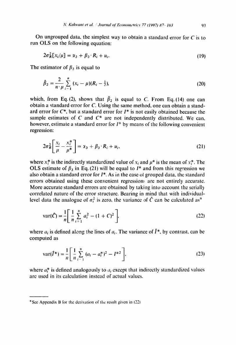
On ungrouped data, the simplest way to obtain a standard error for C is to run OLS on the following equation:

2a 2[xdp] = ~2 + fl,_" R~ + u~. (19)

The estimator of f12 is equal to

f12 ~ 2 " n'# ~ ( x , - - #)(Ri - ~), (20) i - - I

which, from Eq.(2), shows that fi2 is equal to C. From Eq.(14) one can obtain a standard error for C. Using the same method, one can obtain a stand- ard error for C*, but a standard error for I* is not easily obtained because the sample estimates of C and C* are not independently distributed. We can, however, estimate a standard error lbr I* by means of the following convenient regression:

~--- ~ 3 -]- f la'Ri + ui~ (21) it*

where x* is the indirectly standardized value ofx~ and #* is the mean of x*. The OLS estimate of f13 in Eq. (21)will be equal to I* and from this regression we also obtain a standard error for I*. As in the case ol grouped data, the standard errors obtained using these convenient regression~ are not entirely accurate. More accurate standard errors are obtained by taking into account the serialt3, correlated nature of the error structure. Bearing in mind that with individual- level data the analogue of cr~ is zero, the wlriance of (" can be calculated as ~

where a~ is defined along the lines of a,. The variance of ]*, by contrast, can be computed as

var(f*) = i-/ I~i-, (23)

where a* is defined analogously to ~ti except that indirectly standardized values arc used in its calculation instead of actual values.

See Appendix B for the derivation of the result given in (22)

94 N. KaAavani et al. / Journal of Econometrics 77 (1997) 87-103

5. Empirical illustrations

In this section we report some empirical illustrations using data from the combined 1980 and 1981 Dutch Health Interview Surveys (HIS). The sample size, after deletion of cases with missing information, is 10,232 persons. Our stratifying variable is pre-tax household income per equivalent adult. 9 We use two widely available indicators of ill-health - chronic illness (a dummy variable indicating the presence or absence of any chronic illness) and self-assessed health (the HIS question being 'How is your health in general?', to which respondents could reply 'good', 'fair', 'varies', and 'poor'). ~° In the case of the former, we simply used the actual values of the variable. In the case of the latter, we have assumed that underlying the categorical self-assessed health variable is a con- tinuous latent ill-health variable with a standard lognormal distribution (cf. Wagstaff and van Doorslaer, 1994a). ~ t

For the purpose of illustrating the methods for grouped data, we have divided the sample into income deciles, in general, the lower deciles suffer somewhat higher levels of ill-health than the higher deciles (Table I). With the exception of the bottom decile, the effect of the standardization is to reduce the mean ill-health levels of the lower income groups and raise those of the upper income groups. The negative values of C, C +, [L and [~+ in Table 2 imply that even after taking into account the demographic structure of the sample, inequalities in health favour the better-off. The values suggest that inequality is more pro- nouneed if health is measured by self-assessed health than if it is measured by chronic illness, t 2 The standardized vartants of C and [I (C + and [J + ) are smaller than the unstandardized variants (C and [I), implying that solne of the inequality in crude morbidity rates is unavoidable and due simply to the age slructure of the sample. The standard errors lbr C + and [~ + are a good deal smaller than those ol" C and [~ this presumably reflects the fact that the direct standardiza- tion reduces the variation in illness rates. The standard errors obtained using the two methods differ somewhat, but not apparently in any predictable way. It

'~ The equivalence scale used is that used by th~ D~. b Central Bureau of Statistics lcl: Schiepcrs, 1988}, The stale takes into account tile number of adui~.,, and children in the household, as well as the age of tile eldest child.

so Our methods could, ofcours¢, be applied with health meast, res othe," than our chosen indicalors: see for instance Bhargava (1994).

z l In effect, we obtain tile values for each ol" tile four categories by dividing up tile area under tile standard Iognormal distribution according to ,,ample proportions hdling into each of tile four categori,"~

~" This ~:~nclusion is consistent with other research where bolh self-assessed heahh and chro~iic illness are measured by dichotomous variables fci', Kttnst et al., 1992: wm Doorslaer, Wagstall, and Rutt~n, 1993). Tile reason is probably that tile chronic illness dichololllous variable insullicientl) captures the underlying differences in the severity of chronic illness IO'Donncll and Propper. I tit) I ~.

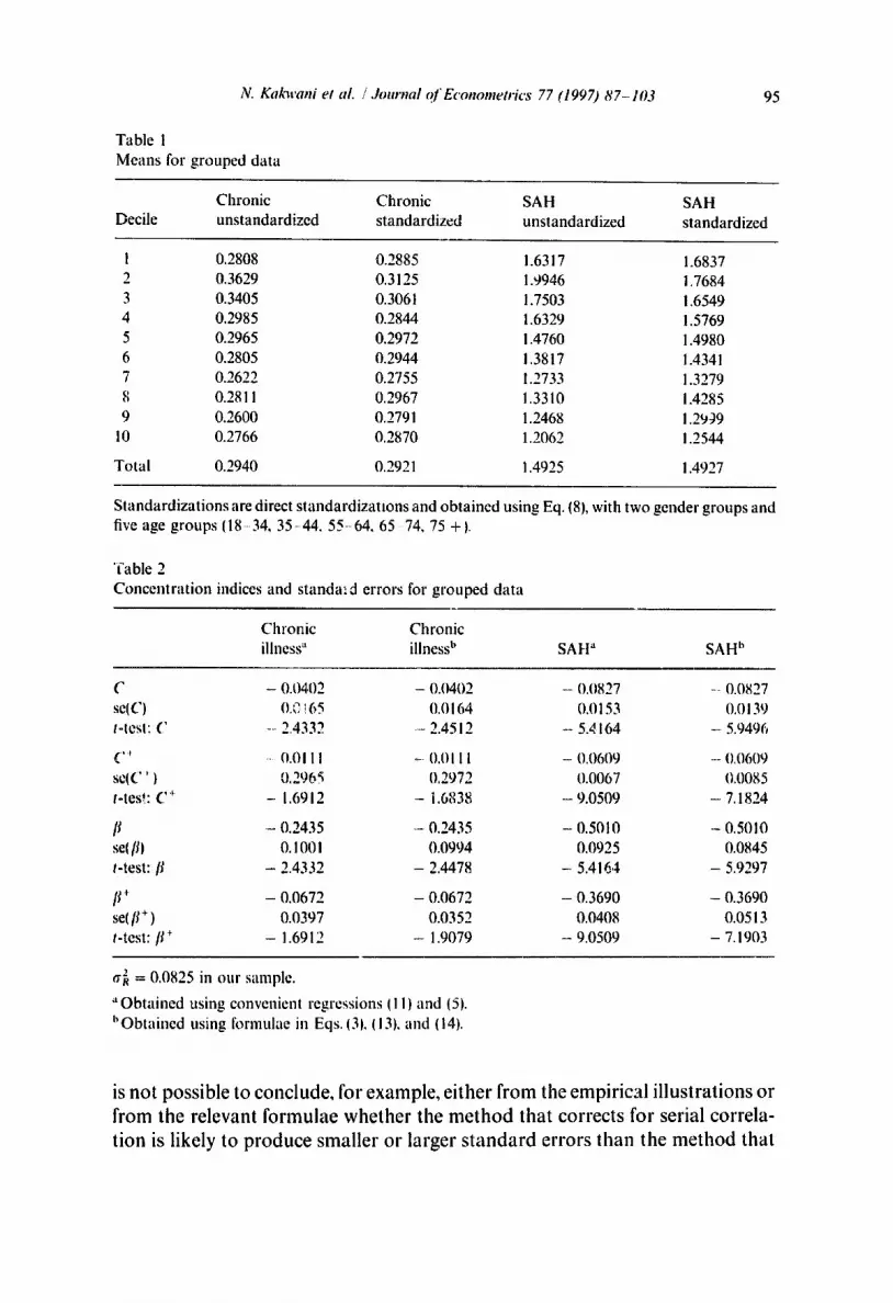
iV. Kakwani et al. / Journal o f Economeo'ics 77 (1997) 8 7 - 1 0 3

Table 1

Means for grouped da ta

95

Chron ic Chron ic SAH SAH

Decile uns tandardized s tandardized uns tandardized s tandardized

1 0.2808 0.2885 1.6317 1.6837 2 0.3629 0.3125 1.9946 i.7684

3 0.3405 0.3061 1.7503 1.6549

4 0.2985 0.2844 1.6329 1.5769

5 0.2965 0.2972 1.4760 1.4980

6 0.2805 0.2944 1.3817 1.4341

7 0.2622 0.2755 1.2733 1.3279

8 0.2811 0.2967 1.3310 i.4285

9 0.2600 0.2791 1.2468 1.2959

10 0.2766 0.2870 1.2062 1.2544

Tota l 0.2940 0.2921 1.4925 1.4927

S tandard iza t ions are direct s tandard iza t ions and ob ta ined using Eq. (8), with two gender groups and five age groups (18 34, 35-44 , 55-64 , 65 74, 75 +1.

"fable 2

Concen t r a t i on indices and standa:cl errors for g rouped da ta

Chron ic Chron ic illness" illness b SA H" SA H h

C - 0.0402 - 0.0402 - 0.0827 ..... 0.0827

seiC) 0.0!65 0.0164 0.0153 0.0139

t-tesl: C --2.4332 - 2.4512 - 5.dl64 ---5.9496

( ..... ~- 0.01 II -- 0.011 I - 0,0609 - 0,0609

s¢(C ' ) 0,296~ 0.2972 (I.0067 0.0085

t-tes!: C + - 1.6912 - 1.6838 - 9.0509 - 7.1824

[I - (I.2435 - 0.2435 - 0.5010 -- 0.5010

se[ [11 O. 1001 0.0994 0.0925 0.0845

t-test: [I - 2.4332 - 2.4478 - 5.4164 - 5.9297

[I + - 0.0672 - 0.0672 - 0.3690 - 0.3690

se( It + ) 0.0397 0.0352 0.0408 0.0513

t-test: [I + - 1.6912 - 1.9079 - 9.0509 - 7.1903

a~ = 0.0825 in our sample.

• ' Ob ta ined using convenient regressions I I I) and (5).

h Ob ta ined using formulae in Eqs. O1, 1131, and (141.

is not possible to conclude, for example, either from the empirical illustrations or from the relevant formulae whether the method that corrects for serial correla- tion is likely to produce smaller or larger standard errors than the method that

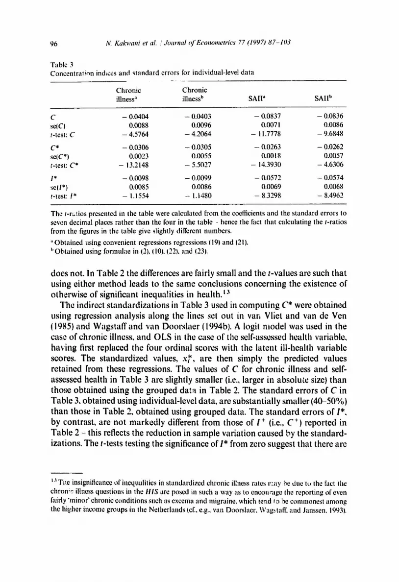
96 N. Kakwani et al. / Journal o f Econometrics 77 (1997) 87-103

Table 3 C o n c e n t r a t i o n ind~ccs and standard errors for individual-level data

C h r o n i c C h r o n i c

i l lness ~ i l lness b S A I l ~ SAII b

C - 0 .0404 - 0 .0403 - 0 .0837 - 0 .0836

se(CI 0.0088 0 .0096 0.0071 0 .0086

t-test: C - 4 .5764 - 4 .2064 - 11.7778 - 9 .6848

C * - 0 .0306 - 0 .0305 - 0 .0263 - 0 .0262

se(C*) 0.0023 0 .0055 0 .0018 0.0057

t-test: C * - 13.2148 - 5.5027 - 14.3930 - 4 .6306

I* - 0 .0098 - 0 .0099 - 0 .0572 - 0 .0574

se(l*) 0.0085 0 .0086 0 .0069 0.0068

t-test: I* - 1.1554 - 1.1480 - 8 . 3 2 9 8 - 8 . 4 9 6 2

The t-ratios presented in the table were calculated from the coefficients and the standard errors to seven decimal places rather than the four in the table - hence the fact that calculating the t-ratios from the figures in the table give slightly different numbers.

" O b t a i n e d us ing c o n v e n i e n t regressions regressions 119~ and (21).

b O b t a i n e d us ing f o r m n l a e in ~2t, I i0~, ~22~, a n d (23j.

does not. In Table 2 the differences are fairly small and the t-values are such that using either method leads to the same conclusions concerning the existence of otherwise of significant inequalities in health.t 3

The indirect standardizations in Table 3 used in computing C* were obtained using regression analysis along the lines set out in van Vliet and van de Ven (1985) and Wagstaff and van Doorslaer (1994bl. A logit model was used in the case of chronic illness, and OLS in the case of the self-assessed health variable, having first replaced the four ordinal scores with the latent ill-health variable scores. The standardized values, x*, are then simply the predicted values retained from these regressions. The values of C for chronic illness and self- assessed health in Table 3 are slightly smaller (i.e., larger in absolute size) than those obtained using the grouped data in Table 2. The standard errors of C in Table 3, obtained using individual-level data, are substantially smaller (40-50%) than those in Table 2, obtained using grouped data. The standard errors of I*, by contrast, are not markedly different from those of i + (i.e., C +) reported in Table 2 - this reflects the reduction in sample variation caused by the standard- izations. The t-tests testing the significance of 1" from zero suggest that there are

t,~ Tt~e ins ign i t i canee o f i a e q u a l i t i e s in s t a n d a r d i z e d c h r o n i c illness rates r: .ay he d u e tu the fact Ihe

c h r o n i c illness questions in the HIS ate posed in s u c h a way as to encotr'age the reporting of even fairly ' m i n o r ' c h r o n i c c ~ m d i t i o n s s u c h as e x c e m a a n d m i g r a i n e , w h i c h t e n d fo I've c o m m o n e s t a m o n g

the hi,t~her i n c o m e g r o u p s in the Netherlands icl:, e.g., van Doorslaer. Wagstaff. and J a n s s e n . 1993).

N. Kakwani et al. /Journal Of Econometrics 77 (1997)87-103 97

no significant avoidable inequalities in the presence of chronic illness but that there are significant avoidable inequalities in self-assessed health. These are the same conclusions that were reached with the grouped data in Section 4, though the t-values for chronic illness are a good deal smaller in the case of I* and I ÷.

6. Conclusions

We have shown that the RII and CI are closely related to one another and that it is possible to construct a variant of the CI to allow inequalities in health to be measured on individual-level data even with age-sex standardization. This allows the extra precision allowed for by individual-level data to be retained but at the same time allows one to net out of one's calculations the unavoidable component of health inequality attributable to the demographic structure of the sample. We have also derived asymptotic distribution-free standard errors for both the RII and the CI. Finally, the empirical illustrations in the paper suggest that there may, in practice, only be small differences between the standard errors obtained using the method which does not take into account serial correlation and those obtained using the method proposed in this paper which does take it into account. Surprisingly, the results also suggest that in this context the gain in precision associated with the use of individual-level data may not always be that large.

Appendix A: Derivation of standard errors based on group( , aata

Suppose there are T socioeconomic groups and .Ii is the population relative frequency of the tth group, then ~/__ 1.Ii = 1. it is reasonable to assume that the sample absoltlte frequencies (hi, n2 . . . . . n.r) based on a sample of n individuals follow a muitinomial distribution so that the means, variances, and covariances of the sample estimates of the relative frequencies are given by

E(.~) =]~, var(.l,t = n.f,(l - J l ) , cov( . /~ , . l l , ) = - -.ft./~.,n if t :/: t',

where t = 1, 2 . . . . . T. Then one can always write

f = . f + ~:, (A. 1 )

where f ' = ( . l l , . I ; . . . . . . /:r), f = ()'l,.r., . . . . . . ~r), and , : '= (,:,, ,:z . . . . . ,:,.), ,: being the error vector such that

E0:) = 0 and E ( d ) = _1 L', (A.2) 11

98 N. Kakwani et al. /Journal of Econometrics 77 (1997) 87-103

2: being the T x T matrix given by

S = d i a g ( f ) - i f ' . (A.3)

Let m' = (~q,/a: . . . . . ~ur), It, being the average morbidi ty of the tth SEG, then the mean morbidi ty of the society is given by

~t = roT. (A.4)

Let fit be the sample estimate of/a,, then one can always write

l~, = l~, + 6,,

where 6, is the error term such that

E(6,) = 0 and E(621 = a/~/n,.

if tfi' = (l~l, fi= . . . . . l~r) and 6' = (fit, 62 . . . . . fir'), then one can write

th = m + 6, (A.5)

such that E ( 6 ) = 0 and E (6 6 ' )= (1/n)t2, where O = d iag(aZ)[d iag( f ) ] -~, tra being the T x 1 vector with the tth element equal to a 2.

A sample estimate of the mean morbidity rate of the society is given by

=

which in view of (A.I) and (A.5) can be written as

ii = ~t + m'~; + f ' 3 , (A.6)

which on assuming that ~: and 6 are independent gives the result: x/~(t~ - i t ) follows normal distribution with mean zero and variance (m'Y,m +f't2j'). This gives the variance of Ii as

l ~ ./;(,u, - ~tt}: + j ; a ~ . (A.7) vart/ ) = -; ,=

Let us now introduce a T x T matrix

A =

! : 0

I 1

1 1

0 , , 0 w

0 ... 0

1 . . . ½

N. Kakwani et ai. / Journal o f Econometrics 77 (Iq o~) 87-103 9 9

which has the property that

A+A'=tt',

where f = (1, 1 . . . . . 1) is the row vector of T elements, each of which being equal to 1.

Let R' = (R~, R2, . . . , RT), R, being the relative rank of the tth SEG (defined in (4)); then R = Af. A sample estimate of R will then be given by/~ = Afwhich from (A. 1) gives

/~ = R + At,. (A.8)

We may now write the sample estimate of the concentration measure C as

t~ = 2 ,h'[diag(.r)]/~ - 1. (a.9) It

Substituting (A.1), (A.5), and (A.8) into (A.9) and applying Taylor's expansion gives

('1' ~ = C + a ' r . + b ' 6 + O p n (A.10)

where

1 a = - [2 diaglR)m + 2,4' diag(./')m - ( I + C)m],

h = / [ 2 d i a g ( f ) R - 11 + C).f],

and Or(l/n)includes all the remainder terms that are of order I/n or less in

probability. Eq.(A.10) immediately gives the result: x / ~ ( C - C) follows an asymptotic normal distribution with zero mean and variance (a'£a + b'Qb) ~'hich gives

I ] + " - T I ~ faor(-R,- I C) 2, (A.II) var(C) =-1 ~ .I;a, 2 - (I + C)-' + ~ , = ,

I1 I = I

where

a , = ~ ( 2 R , - l - C ) + 2 - q , - t - q , and It

being the ordinate of the concentration curve.

'k q, = -~ /,~.lr, (A.12)

100 N. Kakwani et al. /.lournal of Econometrics 77 (1997)87-103

The relative index of inequality RII, which we denote by fl, is related to the concentration as fl = C/2tr 2, where 0 .2 = ~T=~ f d R , - ½)2 (Eq. (6)). A sample estimate of/3 is given by

fi = C'/2~ 2 ,

where

T a~ = y y , ( ~ , _ ½)2.

t = l

Utilizing (A.8) and (A.10~ into (A.13) and Taylor's expansion gave

var(~) = ,,tr----~ ,= ,Z J; e2 - ,= ,Z f ,e , + - ~ ,= , tr 2 R , -

where

t

a ' - f i l ' l + R , ~ - s , - s , _ , ] , s,= Ef.R.. So=0. r = l

(A.13)

- -~ , (a.14)

(A.15)

Similarly, if the sample estimate of standardized C* can be written as

¢* = c* + a'*~. + o . (~) . (A.16)

where the tth element of a* is given by

+

a* = ~ ( 2 R , - 1 - C*) + 2 - q* - q*_l, It

(A.17)

where ltt+ and /.t + are the standardized morbidity means (l/it+)~t__. t ,u~ + J~' is the ordinate of the concentration curve L*(s).

A sample estimate of 1" will then be given by

and q* =

f . = ~ - ¢ . (A.18)

~ = C + a't :+ Op(~) .

If we assume that the groups are homogeneous (which is the case when individual observations are available), tr~ will be zero in each group. The formulae of var(~) and var(fl) will simplify considerably. In this situation,

given in (A.10) will be given by

N. Ka~avani et al. / Journal of Econometrics 77 0997) 87-103 101

which in view of (A.15) and (A.16) becomes

O ( ' ) l * = I * + ( a - a * ) ' g + P n "

This immediately lead to the result that x/~(f* - I * ) follows an asymptotic normal distribution with variance equal to (a - a*)Z(a - a*), which gives

Appendix B: Derivation of standard errors based on individual observations

Eq. (A. 11 ) provides the standard errors of ~ computed on the basis of grouped data. We may now give an alternative derivation of the variance of ( estimated on the basis of individual observations. C can be written as

2 n

xi/~i 1, (B.1) = n~ i - - ,

where x~ is the ill-health score of the ith individual and /~ = (2i - 1 ) /2n , where i is the ith rank when individuals in the sample are arranged in ascending order of x~. It will be useful to write (B.I) as

¢ = ,1/2j~,, IB.2~

where

a = !- ~ 7 i , Il l= 1

qi = Xj X.i. j= l j=

Then following Fraser (1957), we obtain

BI

1 y, Ix, - i~) 2, . v~rt;2) = ~ ~=,

n v~r(~) = 4_ ~ (at - a ) 2, H i = I

near(a . ~) = -2 ~ (x~ - l~l(a~ - at. 17 i= !

102 N. Kai[nt'ani et al. / Journal of Econometrics 77 (1997) 87-103

Then applying the 6 method given in Rao (1965, p. 321) the estimated variance of C" from (B.2) is obtained as

1 [var(a) + 4C 2 vfir([i) - 4Cc6v(J, i~)] v r(CT) =

I - E (c7, - c7 -- Cx i + C'xi + 8 ~ ) 2. (B.3) 4~2n

i = l

Note that one can also derive vfir(C) from Eq. (A.11) by substituting ¢r~ = 0 which gives

vfir(C) = _1 ~, (ai - 1 - 8) , (B.4) ~l i = l

where

a~ = x4 (2/~ - 1 - 8) + 2 - q, - q; - , . It

Comparing (B.3) and (B.4) we note that the two expressions are identical. Thus, the two alternative derivation of the standard errors give identical results.

References

Bhargava. Aiok, 1994, Modelling tile health of Filipino chindren, Journal of tile Royal Statistical Society A 157, Part 3.

Cowcll, F,A., 1989, Sampling wu'iauc¢ and decomposable inequality measures, Journal of Econo- metrics 42, 2 7 4 1 .

Doorslacr, E. van, A. Wag:~tafl', and F. Rutlen, eds., 1993a, Equity in the finance and delivery of health care: An international prospective (Oxford University Press, Oxlbrd).

Doorslacr, E. van, A. Wagstaff, and R. Janssen, 1993b, Equity in the finance and delivery of health care in the Netherlands, in: E. van Doorslacr, A. Wagstaff, and F. Rutten, eds., Equity in the finance and delivery of health care: An international perspective (Oxlbrd University Press, Oxford).

Fraser, 1957, Non-parametric methods in statistics (New York, NY). Hocffding, W., 1948, A class of statistics with asymptotic normal distribution, Annals of Mathemat-

ical Statistics XIX, 293-325. lilsley, R. and J. Lc Grand, 1987, The mcasurcmcnt of inequality in health, in: A. Williams, cd.,

Health and economics {Macmillan, London). Jenkins, S., 1986, Calculating income distribution indices from .nicrodata, National Tax Journal 61,

139-142. Kakwani, N.C., 1977, Measurement of tax progessivity: An intcrnatioual comparison, Economic

Journal 87, 71 80. Ki, kwani, N,C., 1980, Income inequality and poverty: Methods of estimation and policy application

{Oxford University Press, New York, NY). Kakwani, N.C,, 1990, Large sample distributions of scveralf inequality measures: With application

to C6te d'Ivoire, in: R.A.L. Carter, J, Dutta, and A. Uilah, eds., Contributions to econometric theory and application (Springer-Vcrlag, New York, NY).

N. Kakwani et al. / Journal of Eco,mmetrics 77 (1997) 87-103 103

Kunst, A.E. and J.P. Mackenbach, 1994, Size of mortality differences associated with educational level in nine industrialized countries. American Journal of Public Health 84, 932-937.

Kunst, A.E., J. Geurts, and L. van den Berg, 1992, International variation in socioeconomic inequalities in self-reported health (Dutch Cemral Bureau of Statistics, Voorburg).

Lambert, P.J., 1993, The distribution and redistribution of income: A mathematical analysis (Manchester University Press, Manchester).

Lerman, R.I. and S. Yitzhaki, 1984, A note on the calculation and interpretation of lhe Gini index, Economics Letters 15, 363-368.

Nyg/ird, F. and A. Sandstr6m, 1981, Measuring income inequality (Almqvist & Wiksell Interna- tional, Stockholm).

O'Donnell, O. and C. Propper, 1991, Equity in the distribution of UK National Health Service resources, Journal of Health Economics 10, i - 19.

Pappas, G., S. Queen, W. ltadden, and G. Fisher, 1993, The increasing disparity in mortality between socioeconomic groups in the United States, 1960 and 1986, New England Journal of Medicine 329, 103-108.

Preston, S.H., M.R. Haines, and E. Pamuk, 1981, Effects of industrialization and urbanization on mortality in developed countries, in: Solicited papers, Vol. 2, IUSSP 19th international popula- tion conference (IUSSP, Liege).

Rap, C.R., 1965, Linear statistical inference and its applications (Wiley, New York, NY). Rothman, K,, 1986, Modern epidemiology (Little, Brown & Co., Boston, MA). Schiepers, J., 1988, Huishoudensequivalententiefactoren volgens de budgetverdelingsmethode,

Sociaal-economische Maandstatistiek Suppl. 7, 28-37. V/iger6, D. and O. Lundberg, 1989, Health inequalities in Britain and Sweden, The Lancet I1, 35--36. Vliet, R. van and W. van de Ven, 1985, Differences in medical consumption between publicly and

privately insured in the Netherlands: Standardization by means of multiple regression, Paper presented to international meeting on health economics (Applied Econometrics Association, Rotterdam).

Wagstaff, A. and E. wm Doorslaer, 1994a, Measuring inequalities in health in the presence of multiple-category morbidity indicators, Health Economics 3, 281 291.

Wagstall: A. and E. van Doorslacr, 1994b, A new approach to the measurement of equity in the delivery of health care, Equity project working paper no. 6 (Erasmu,~ University, Rotterdam).

Wagstafl: A., E. van Doorslaer, and P. Paci, 1989, Equity in the linance and delivery of health care: Some tentative cross-country comparisons, Oxford Review of Economic Policy 5, 89 112.

Wagstaff, A., P. Paci, and E. van Doorslaer, 1991, On the measuremenl of inequalities in health, Social Science and Medicine 33, 545 -557.