DISCUSSION PAPER SERIES

IZA DP No. 13682

Joshua D. Merfeld

Smallholders, Market Failures, and Agricultural Production: Evidence from India

SEPTEMBER 2020

Any opinions expressed in this paper are those of the author(s) and not those of IZA. Research published in this series may include views on policy, but IZA takes no institutional policy positions. The IZA research network is committed to the IZA Guiding Principles of Research Integrity.The IZA Institute of Labor Economics is an independent economic research institute that conducts research in labor economics and offers evidence-based policy advice on labor market issues. Supported by the Deutsche Post Foundation, IZA runs the world’s largest network of economists, whose research aims to provide answers to the global labor market challenges of our time. Our key objective is to build bridges between academic research, policymakers and society.IZA Discussion Papers often represent preliminary work and are circulated to encourage discussion. Citation of such a paper should account for its provisional character. A revised version may be available directly from the author.

Schaumburg-Lippe-Straße 5–953113 Bonn, Germany

Phone: +49-228-3894-0Email: publications@iza.org www.iza.org

IZA – Institute of Labor Economics

DISCUSSION PAPER SERIES

ISSN: 2365-9793

IZA DP No. 13682

Smallholders, Market Failures, and Agricultural Production: Evidence from India

SEPTEMBER 2020

Joshua D. MerfeldKDI School of Public Policy and Management and IZA

ABSTRACT

IZA DP No. 13682 SEPTEMBER 2020

Smallholders, Market Failures, and Agricultural Production: Evidence from India*

Market completeness has important implications for household behavior. I firmly reject

complete markets for smallholders but am unable to do so for non-smallholders. This

leads to important differences in production behavior: smallholders reallocate labor across

activities less in response to intra-seasonal crop price changes than do non-smallholders.

A counterfactual exercise indicates smallholders could increase revenue by almost nine

percent if they were to reallocate labor similarly to non-smallholders. The overall pattern of

results is consistent with small-holders lacking sufficient wage employment opportunities.

Since non-smallholders have to hire in for agricultural production, this lack of opportunities

does not affect their decisions.

JEL Classification: J20, J43, O13, Q12, Q13

Keywords: markets, market failures, agriculture, labor

Corresponding author:Joshua D. MerfeldKDI School of Public Policy and Management263 Namsejong-roSejong-siSouth Korea

E-mail: merfeld@kdis.ac.kr

* I am indebted to Leah Bevis, Marc Bellemare, Rajeev Dehejia, Alex Eble, Jonathan Morduch, Martin Rotemberg,

and Debraj Ray for discussions and comments. Seminar participants at NYU, Columbia, and the KER conference

provided helpful comments. All remaining errors are my own.

1 Introduction

Do households act as if markets are complete? While earlier research was less conclusive

(Benjamin, 1992), the more recent papers in this body of literature consistently reject

market completeness in a diverse set of circumstances, including sub-Saharan Africa

(Dillon andBarrett, 2017;Dillon et al., 2019) and southeastAsia (LaFave andThomas, 2016).

However, while these results contribute to our understanding of market structure in these

countries, little work has examined some of the implications of these specific findings

of market (in)completeness.1 This paper contributes to and extends this literature by

empirically testing predictions for agricultural production in the face of market failures.2

In addition, treating market failures as a household-specific phenomenon allows for a

better understanding of exactly what kinds of markets appear to be failing and for which

households.

An important feature of agricultural households is that they are both producers and

consumers of the same good. This feature is described in the classical agricultural house-

hold model (Singh et al., 1986). In the canonical model under common assumptions,

production and consumption decisions are separable. In other words, households are

able to first make production decisions to maximize profits and then make consump-

tion decisions. Importantly, this implies that production decisions are independent of

consumption decisions and, thus, that household consumption preferences do not affect

production decisions. This is a powerful simplification that underlies a number of influ-

ential studies into many different facets of household behavior. Both LaFave and Thomas

(2016) and LaFave et al. (2018) enumerate a (non-exhaustive) list of some of these studies,

which include: the operation of markets (Jayachandran, 2006; Kaur, 2019; Rosenzweig,

1980); nutrition, intrahousehold allocation of resources, and productivity (Strauss, 1984;

1Importantly, it is not a question of whether markets are incomplete, but rather whether household behaveas if markets are incomplete.

2Previous theoretical and empirical research has examined the impacts of market failures on productiondecisions (de Janvry et al., 1991; Taylor and Adelman, 2003), including when labor markets are incomplete(Sadoulet et al., 1998).

2

Udry, 1996); technology adoption (de Janvry et al., 1991; Conley and Udry, 2010; Suri,

2011); risk (Townsend, 1994; Jacoby and Skoufias, 1997); and, perhaps most pertinent

to the present study, wage determination and labor supply (Barnum and Squire, 1979;

Strauss, 1986; Kochar, 1999).

However, the recursion property rests on a number of stringent assumptions, one of

which is complete markets.3 Yet, there is ample evidence that markets are not complete in

developing countries. The most direct evidence comes directly from tests of the recursion

property itself. Benjamin (1992) was the first to note that recursion implies production

decisions should be independent of any household characteristics that affect only con-

sumption, like demographic characteristics. As such, a straightforward test for market

completeness is to regress total farm labor on household demographics; under the null hy-

pothesis of complete markets, household demographics should not affect total farm labor

demand and the vector of coefficientswill be zero. Rejection of this hypothesis implies that

markets are not complete. While Benjamin (1992) was unable to reject complete markets,

more recent literature unequivocally challenges this finding; Dillon and Barrett (2017),

Dillon et al. (2019), and LaFave and Thomas (2016) all strongly reject market completeness

in multiple contexts.

Importantly, however, these results provide little intuition into what markets may be

failing or why.4 Moreover, this omnibus test does not yield any insight into how market

failures may impact farmer decision-making. In this paper, I provide empirical evidence

of some of the implications ofmarket failures for agricultural production in India. In other

words, I ask: what can we say about howmarkets – or the lack thereof – affect production

decisions made by Indian households? While answering this question, I also provide

one of the first direct tests of market failures in the Indian context and present additional

evidence that market failures are a household-specific phenomenon; while I reject that

3For example, recursion also relies on perfect substitution of family and hired labor as well as no preferencesfor working on one’s own farm.

4Dillon et al. (2019) is an exception. The authors explore asymmetric labor responses in an attempt to shedmore light on the functioning of specific markets.

3

smallholders behave as if markets are complete, I am unable to reject this hypothesis for

non-smallholders, consistent with recent evidence from Indonesia (LaFave et al., 2018).

Taking these results at face value, I then analyze whether smallholders and non-

smallholders behave as predicted by economic theory. If smallholders behave as ifmarkets

are incomplete but non-smallholders do not, economic theory predicts that labor elasticity,

with respect to crop prices, should be lower for smallholders. To test this prediction, I use

five years of high-frequency data from ICRISAT’s Village Dynamics in South Asia (VDSA)

project. The data contain monthly data on labor allocation, wages, and crop prices. I

first implement the classical test of Benjamin (1992) and LaFave and Thomas (2016) by

regressing total farm labor on a vector of household demographic characteristics. Results

strongly reject recursion – and, thus, that households behave as if markets are complete

– for smallholders but fail to reject recursion for non-smallholders. I then empirically

test the theoretical predictions. Identification comes from within-season reallocation of

labor across different activities. I condition on all planting decisions and examine how

households reallocate labor in response to price changes between planting and harvesting.

After first confirming that households do indeed reallocate labor in response to changes

in crop priceswithin the agricultural season, I then test the themain theoretical prediction.

The evidence clearly indicates that smallholder households respond less to intra-seasonal

crop price changes than do non-smallholders. Moreover, the patterns suggest that small-

holders have excess labor butmay lack off-farm employment opportunities. I also perform

a simple counterfactual exercise to estimate how much labor reallocation increases sea-

sonal output. If smallholders were able to reallocate labor in response to price changes,

like non-smallholders, revenue on the plots included in this study would be almost nine

percent higher.

Additional results using labor allocated to non-agricultural activities provides addi-

tional evidence of how markets may fail for smallholders. In particular, an (unexpected)

increase in crop price induces smallholders to report lower levels of involuntary unem-

4

ployment but does not affect their allocation to wage employment. This is consistent

with a story in which a decrease in crop prices leads smallholders to reallocate time to

(unsuccessfully) search for off-farm wage labor. Importantly, non-smallholders do not

reallocate labor to these two non-agricultural activities in response to changes in crop

prices; the coefficients are not only insignificant but also small in magnitude. While none

of the evidence comes from direct tests of which markets are failing, the overall evidence

points to an environment in which smallholders overallocate labor to agricultural pro-

duction. Consistent with this story, the number of acres-per-person is much higher for

non-smallholders than smallholders. This is consistent with non-smallholders behaving

as if markets are complete but with smallholders behaving as if they are not. In other

words, it appears that non-smallholders may be able to hire in whenever they are in need

of additional labor, but that smallholders are not always able to find wage employment,

leading them to allocate their excess labor to agricultural production.

This paper contributes to several lines of literature. Most obviously, this paper extends

the literature testing for market completeness using the agricultural household model

(Benjamin, 1992; Dillon and Barrett, 2017; Dillon et al., 2019; LaFave and Thomas, 2016).

In addition to providing evidence of market completeness in India in a more general

sense, I also argue that market failures are a household-specific, not market-specific,

phenomenon. This is consistent with other contemporaneous evidence from Indonesia

(LaFave et al., 2018). While this is not a new argument, this paper offers clear empirical

evidence of some of the implications of household-specific market failures.

Other research that does not explicitly test formarket completeness nonetheless presents

evidence consistentwith incompletemarkets. For example, findings that the shadowwage

differs across activities is not consistent with the complete-markets case (Brummund and

Merfeld, 2019; Jacoby, 1993; Skoufias, 1994). This paper extends earlier empirical and

theoretical literature on the implications of market failures (de Janvry et al., 1991; Sadoulet

et al., 1998; Taylor and Adelman, 2003) by leveraging arguably exogenous variations in

5

prices between planting and harvest to examine how households respond when markets

are incomplete.

The rest of this paper is organized as follows. The next section elaborates a theoretical

model of how market completeness affects household production decisions. Section 3

discusses the data and methodology, including summary statistics. Section 4 presents the

main results and Section 5 concludes.

2 Separation and Agricultural Production

Consider an agricultural household that maximizes its own utility, subject to agricultural

production and a possible off-farm labor constraint. Consumption, c and leisure l, are the

arguments in the household’s utility function. The household operates i > 0 plots and

allocates its own labor to any of those plots, LFi , and wage labor, Lw , subject to possible

constraint on total wage labor supplied off-farm, Lw . Thus, the household’s total time

endowment is L � l +∑

i LFi + Lw . The household can also hire in labor, LH

i , where i again

indexes different plots.

Thus, the household’s problem is:

max E[u(c , l | γi)

], subject to : (1)

c ≤∑

i

pi fi(LFi + LH

i ; Ai)γi + w(Lw −∑

i

LHi ) (2)

L ≥ l +∑

i

LFi + Lw (3)

Lw ≥ Lw (4)

0 ≤ LHi , L

Fi , Lw , l , (5)

where γi is a multiplicative productivity shock, pi is the price of the crop grown on plot

6

i, and w is the wage. The expectation is taken across γ. Due to my identification strategy,

I model this as a static problem. The strategy focuses on intraseasonal labor reallocations

across plots and, thus, land is fixed during the relevant period.

The assumption of complete markets is very useful analytically. As previously shown

(Benjamin, 1992; Dillon et al., 2019; LaFave and Thomas, 2016), complete markets allow

households to separateproductiondecisions fromconsumptiondecisions. In effect, house-

holds first maximize farm profits before making consumption decisions. The household’s

production decisions can thus be modeled as:

max E

[∑i

pi fi(Li ; Ai)γi + w(Lw −∑

i

LHi )

]≡ π∗. (6)

Powerfully, this means that total farm labor, LTotal , is only a function of prices:

LTotal∗� LTotal∗(pi , w | γi) (7)

This prediction has formed the basis of most tests for complete markets. When markets

are complete, total farm labor is uncorrelatedwith household consumption characteristics,

such as household demographic variables. This is the basis for the first test in this paper,

which follows LaFave and Thomas (2016) and which I describe in detail in section 3.

However, there are additional implications on the production side of market complet-

ness. In particular, the profit function itself implies a number of specific relationships

across variables. First, consider the first-order conditions for total labor demand on a plot

after the productivity shock has been realized5:

5This assumption is compatible with the identification strategy used in this paper, which I elaborate below.

7

pi∂ fi

∂Liγi � w. (8)

Importantly, conditional on the price of crop i and the market wage, the price of crop

j , i does not affect labor demanded on plot i. Intuitively, this is driven by the fact that

each plot’s labor choice is driven by equality of the marginal revenue product of labor

(MRPL) with the market wage. A change in the price of crop j will affect the MRPL of

labor on plot j, but will not affect the MRPL of labor on plot i. Consider now a world in

which the off-farm labor constraint (equation 4) is binding.6 The first-order conditions are

now,

pi∂ fi

∂Liγi � w∗ � p j

∂ f j

∂L jγj , (9)

where w∗ is the household shadow wage, which need not equal the market wage. Unlike

the market wage, the shadow wage is directly affected by labor reallocations across pro-

ductive activities within a household.7 Suppose p j increases, simultaneously increasing

the MRPL of L j . To bring the household back to an optimal allocation of labor, the house-

hold must increase L j in order to bring MRPL j back to equality with other labor uses. At

the same time, given the market constraint – and the fact that households for whom Lw

binds do not simultaneously hire labor – households must allocate labor away from other

activities. In the current model, this would be l and Li . Thus, an increase in p j affects both

Li and l, whereas neither is affected when markets are complete.

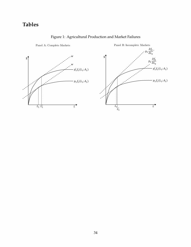
Figure 1 presents a graphical explanation of this. Panel A shows the change in Li when

6More generally, at least two markets are required to fail if we are to observe non-separation in the data.7Indeed, the shadow wage is defined as being equal to the MRPL at the optimum. In the complete-marketcase, on the other hand, the optimal MRPL is determined by the market wage itself, and labor is onlyreallocated to bring the MRPL back into line with the wage.

8

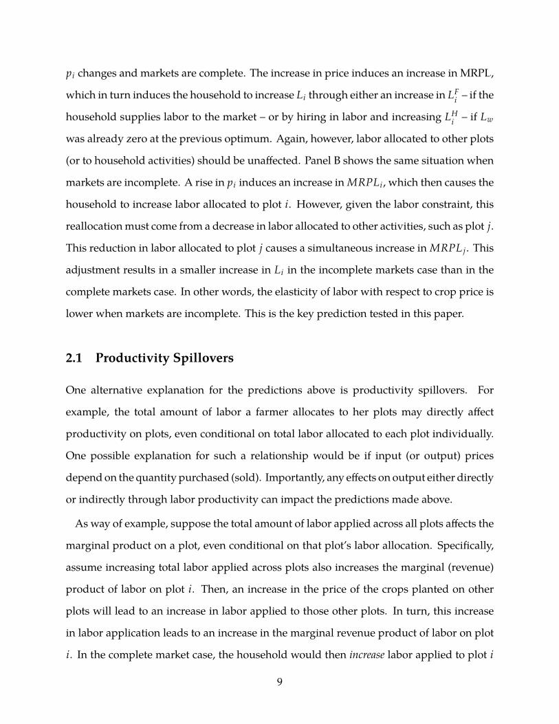
pi changes and markets are complete. The increase in price induces an increase in MRPL,

which in turn induces the household to increase Li through either an increase in LFi – if the

household supplies labor to the market – or by hiring in labor and increasing LHi – if Lw

was already zero at the previous optimum. Again, however, labor allocated to other plots

(or to household activities) should be unaffected. Panel B shows the same situation when

markets are incomplete. A rise in pi induces an increase in MRPLi , which then causes the

household to increase labor allocated to plot i. However, given the labor constraint, this

reallocationmust come from a decrease in labor allocated to other activities, such as plot j.

This reduction in labor allocated to plot j causes a simultaneous increase in MRPL j . This

adjustment results in a smaller increase in Li in the incomplete markets case than in the

complete markets case. In other words, the elasticity of labor with respect to crop price is

lower when markets are incomplete. This is the key prediction tested in this paper.

2.1 Productivity Spillovers

One alternative explanation for the predictions above is productivity spillovers. For

example, the total amount of labor a farmer allocates to her plots may directly affect

productivity on plots, even conditional on total labor allocated to each plot individually.

One possible explanation for such a relationship would be if input (or output) prices

depend on the quantity purchased (sold). Importantly, any effects on output either directly

or indirectly through labor productivity can impact the predictions made above.

As way of example, suppose the total amount of labor applied across all plots affects the

marginal product on a plot, even conditional on that plot’s labor allocation. Specifically,

assume increasing total labor applied across plots also increases the marginal (revenue)

product of labor on plot i. Then, an increase in the price of the crops planted on other

plots will lead to an increase in labor applied to those other plots. In turn, this increase

in labor application leads to an increase in the marginal revenue product of labor on plot

i. In the complete market case, the household would then increase labor applied to plot i

9

to re-equate MRPL on that plot with the market wage. In the incomplete market case, on

the other hand, this would lead to less of a reallocation of labor away from plot i. To test

for these possibilities, I test for spillovers of this type in the results section below.

2.2 Efficiency of Family and Hired Labor

Another alternative, explicated in Benjamin (1992), is that family and hired labor have

different prices. This could be driven, for example, by differing efficiencies of family and

hired labor. There are two possibilities. First, consider a situation in which family labor is

less efficient than hired labor. In this case, the household’s profit-making labor allocation

is to allocate family labor completely to themarket, until the point that themarginal utility

of an additional hour of work is equated with the marginal utility of an additional hour

of leisure, with consumption being the relevant trade-off between the two. Importantly,

the predictions above are unchanged, as separation still occurs: the household maximizes

on-farm profits by allocating only hired labor to agricultural production, up to the point

that the MRPL of that hired labor equals their wage.

The second case, in which family labor is more efficient than hired labor, is different.

Following Benjamin (1992), assume family and hired labor are perfectly substitutable, but

one hour of hired labor is equal to α hours of family labor. Thus, we can write total family

labor-efficient units as:

LFe � LF

+ αLH . (10)

Importantly, the exactmix of family andhired laborwill dependonhouseholdpreferences;

separation does not occur. However, the total efficiency units of labor do not depend on

household preferences. Rather, they are determined by the first-order conditions (Benjamin,

1992). Thus, for a given α and a given LFe , the total amount of labor applied will be

unchanged across plots, within the household.

10

This is a key point for this paper, as we can model profit-maximizing labor allocation

decisions as plot-specific. In other words, a change in the price of a crop on plot j , i

does not change the first-order conditions for profit maximization on plot i. As such, the

general predictions explicated above should hold here, as well.

3 Data and Empirical Strategy

This paper uses ICRISAT’s Village Dynamics in South Asia (VDSA) data.8 ICRISAT has

been collecting longitudinal data in India for several decades, but I use the most recent

longitudinal data, which spans the years 2010 to 2014. My final sample, which I describe

in more detail below, comprises 1,089 different households across 17 districts in 8 different

states. Importantly, the data contains monthly-level information on labor and resource

allocation across agricultural plots for the entire five years of the panel. Data is collected

monthly, so recall is minimized. In addition, the village data collects information on

individual crop prices relevant for local farmers, also at monthly intervals, which plays

an important role in the empirical strategy I employ. Finally, five separate years of data

remove some concerns regarding the heterogeneity of effectswhen populations are subject

to aggregate shocks (Rosenzweig and Udry, 2020).

3.1 Empirical Strategy and Identification

This paper approaches the question of separation and complete markets in several ways,

making use of the rich panel data. Since I use household-level fixed effects, all regressions

cluster standard errors at the household level unless otherwise reported. First, I borrow

specifications from prior literature and analyze whether household demographics predict

farm-level labor demand (Benjamin, 1992; Dillon and Barrett, 2017; Dillon et al., 2019;

LaFave and Thomas, 2016). I diverge from the prior literature in two key ways. First, five

8http://vdsa.icrisat.ac.in/vdsa-index.htm

11

years of panel data allow me to employ fixed effects at much lower levels of aggregation

than other literature. In particular, I am able to estimate regressions using household-

plot-crop fixed effects, which restricts attention only to plots plantedwith the same crop in

multiple years. Second, much of the previous literature has used data from Africa (Dillon

and Barrett, 2017; Dillon et al., 2019) or Indonesia (Benjamin, 1992; LaFave and Thomas,

2016), whereas the ICRISAT VDSA data was collected in India.

I first explore the relationship between household demographics and plot-level labor

demand:

lo gLikt � αcik + γvtdc + Xikt + rainvt + β(ΣGg�1δgkt) + εikt , (11)

where lo gLikt is log of total labor applied to plot i in household k in season t, αcik is

household-plot-crop fixed effects, γvtdc is village-wave-season-crop fixed effects, Xikt is

a vector of time-variant plot characteristics – area planted and area irrigated – rainvt is

total rainfall in village v in season t, δgkt is a group of variables indicating the number

of household members that reside in the household in each demographic group g, and

εikt is a mean-zero error term. Following previous literature, the assumption of complete

markets implies that β is a vector of zeros, that is, that demographic variables do not

belong in the labor-demand equation. Thus, the null hypothesis is that β � 0, and F is

the appropriate test statistic. I split household members into five separate demographic

groups: prime-age males (15-59), prime-age females, elderly males (60+), elderly females,

and children (<15). The main specifications include log of household size along with

shares of four of the five demographic groups, with children being the omitted category.

I also test robustness to alternative demographic definitions.

Identification here relies on there being no unobserved time-variant variables correlated

with the error term and the demographic variables. The village-wave-season-crop fixed

12

effects help alleviate any concerns that crop-specific aggregate village shocks in a given

season are correlatedwith household size and total labor allocation. This could be the case

if, for example, shocks lead to changes in migration. Household-plot-crop fixed effects

alleviate additional concerns related to the endogeneity of household size, crop choice,

and area planted. For example, if changes in household size are correlated with planting

decisions – perhaps a larger household will decide to plant a larger area – then controlling

for area planted may actually lead to biased demographic coefficients. While this would

be a clear rejection of the separation hypothesis, if the effect of demographics on labor

demand operates completely through area planted, then the bias might lead to a failure

to reject the null hypothesis if we control for area planted. The fixed effects help alleviate

this concern.

While the previous literature on separation and market failures has pooled all house-

holds, market failures are in fact a household-specific phenomenon. Just because one

household has access to credit, for example, does not imply that other households in

the immediate vicinity also have access to credit. As such, pooling all households may

give a misleading picture of the context of household behavior. One variable that may

be correlated with access to markets is landholdings. As such, I estimate Equation 11

separately for smallholders and non-smallholders, as defined by the survey. Smallholders

are defined as landholders in the lowest two brackets of the landholding distribution. de-

mogsums1 presents summary statistics of some of the differences between smallholders

and non-smallholders in the VDSA data.

The predictions of the model relate to how households respond to changes in prices. It

is difficult to find exogenous variation in prices with respect to household labor allocation

and output at an aggregate level. As such, I focus on individual households and how

they reallocate labor across plots within the agricultural season. In particular, I focus on

monocropped plots – plots planted with just a single crop – and examine how households

reallocate labor when the price of one crop changes relative to the price of another crop on

13

that household’s own plots. Before testing the predictions of the model, I first verify that

households do indeed reallocate labor across plots in response to changes in crop prices.

I estimate:

lo gLikm y � αcik + γdymc + Xikm y + Zikt + rainvm y + βlo gPymvc + εikm y , (12)

where lo gLikm y is log of non-planting and non-harvest labor allocated to plot i in house-

hold k in month m in year y, αcik is household-plot-cropped fixed effects, γdymc is district-

year-month-crop fixed effects, Xikm y is a vector of characteristics that vary by month

(specifically, the amount of labor and materials that had been allocated to that plot in

that season up to that point), Zikt is a vector of planting hours and planting materials in

that season, and lo gPymvc is the monthly price of the crop planted on that plot, which is

defined at the village level. In some specifications, I allow the effects of X, Y, and rain to

vary by the month of the year. In this specification, the coefficient of interest is β; it shows

the effect of a change in the crop price on labor allocation at the plot level. For labor, note

that this includes both family labor and hired labor. Perhaps unsurprisingly, hired labor

is much more common for non-smallholder households.

Themain hypotheses relate to how households respond to changes in crop price, similar

to the specification in Equation 12. To this end, many of the specifications are simple

variations on Equation 12. For prediction one, I restrict attention to households with just

two separate crops. I add an additional variable to the specification, which is the price of

the second crop grown by the household (that is, the price of the crop that is not grown

on plot i). For the other two predictions, I interact the crop price dummy (lo gPcvm y) with

a dummy for smallholder (prediction two) or with both a dummy for smallholder and the

number of crops grown by the household (prediction three).

14

3.2 Identification

This paper explores how households respond to change in crop prices within the agri-

cultural season. One advantage of this strategy is that area planted is necessarily fixed

after the planting season, avoiding one complication. However, the key drawback is that

household labor allocation and crop prices may be endogenous. Most obviously, they

may both be responding to (expected) temporal changes in the agricultural season or a

shared cause, like rainfall. What my empirical strategy needs to accomplish is to purge

any expected changes in crop prices, as well as any spurious causation caused by other

variables. In essence, I need the crop price variable to represent unexpected changes in the

crop price for any given household.

To accomplish this, the identification strategy relies heavily on fixed effects. Within

variation comes from district-year-month-crop fixed effects. Since all households in a

district will be similarly affected by aggregate shocks for a given crop, identification

comes from unexpected differences in the price for a single crop across villages within

a district. This helps purge any possibility that households change plots based on pre-

planting signals – like weather forecasts (Rosenzweig and Udry, 2014, 2019). Also note

that permanent differences in prices for a given crop in different villages within the same

district are swept out by the household-plot-crop fixed effects.9

Since identification comes from within-season variation in crop prices, I control for all

previous plot-level decisions. This includes the number of hours and materials used

during planting as well as the sum of all previous hours and materials allocated to the

plot between planting and the month of observation. Controlling for previous decisions

should help alleviate any concerns that cyclical patterns are driving decisions, in addition

to the fixed effects. In most specifications, the effect of previous hours and materials are

9The district-year-month-crop fixed effects are also important to sweep out aggregate correlations in prices,output, and labor allocation driven by weather. Table A1 shows that in a simple cross-section regressiontotal output, at the plot level, is highly negatively correlated with harvest price. This is likely driven bythe fact that poor output driven by weather shocks often leads to higher crop prices. However, once weinclude the district-year-month-crop fixed effects, this negative correlation disappears.

15

allowed to vary by the month of the year. I also include monthly rainfall totals, which

are also allowed to vary by the month of the year, since the timing of rainfall is especially

important in rain-fed agriculture.

Since croppricesvaryat thevillage-crop level andboth smallholders andnon-smallholders

reside in each village, it is unlikely that differences in the predictive power of crop prices

alone can explain the results. Nonetheless, if there is heterogeneity in themake-up of each

village, this is possible. Appendix Table A2 shows that, at the plot level, lagged crop prices

are equally predictive of current crop prices for both smallholders and non-smallholders.

In other words, any differential reactions to price changes are not driven by differences in

the predictive power of prices for different households.

A short discussion of what actually drives the (unexpected) crop price changes is war-

ranted. At first glance, one might wonder whether this is simply noise. However, certain

households in the sample, non-smallholders, respond very strongly to these signals, sug-

gesting noise cannot alone explain the variation. Within-country price variation persists

in developing countries (Osborne, 2004; Chatterjee and Kapur, 2016; Zant, 2018), even

in countries like India, which has invested significant amounts of money in improving

infrastructure (Bellemare et al., 2013; Chatterjee and Kapur, 2016). In India, specifically,

much of this variation may be driven by strict laws governing where farmers are able to

market their agricultural output; farmers are generally only allowed to market output in

the state in which they live, leading to cross-border discontinuities in prices, despite geo-

graphic proximity (Chatterjee, 2019). This does not, however, explain intra-state variation

in prices. Instead, a look towards infrastructure may provide a partial answer. Though I

control for village-specific rainfall, I do not control for rainfall and general agricultural pro-

ductivity conditions in areas to which a given village is connected. Idiosyncratic changes

in connected villages may drive similarly idiosyncratic changes in a given village. In fact,

previous research has shown that just how one village is connected to other areas plays

an important roll in price variation (Zant, 2018).

16

3.3 Summary Statistics

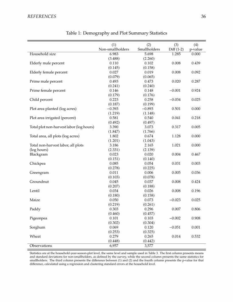
Table 1 presents summary statistics for a number of different variables, broken down

by smallholder status. Note that observations are at the household-plot level, the same

level at which Equation 11 is estimated. First, note that non-smallholders actually have

larger households, on average, than smallholders. The demographic breakdown of the

households are somewhat similar, though it appears that non-smallholders have slightly

more prime-age female and smallholders have slightly more children.

Onaverage, actual plots are larger, in termsof areaplanted, for non-smallholders, though

theydonot appearmore likely tobe irrigated, at least as apercentageof theplot. Consistent

with this, non-smallholders also allocate more hours to these large plots. However, hours

do not increase as much as area when comparing non-smallholders and smallholders,

suggesting smallholder plots may be cultivated more intensively than non-smallholder

plots, consistent with previous research. While individual plots are approximately 65

percent larger for non-smallholders, overall area planted is even higher, approximately

three times larger than smallholder area planted.

Crop choice is somewhat similar across household types, though there are some differ-

ences. The highest average price per kg is highest for green gram, and non-smallholder

plots are slightly more likely to be planted with green gram. Chickpea and pigeonpea are

also higher-priced crops, and non-smallholder plots are more likely to grow the former,

but not the latter. However, the most commonly grown crops, paddy and wheat – which

together make up more than half of all plots – are equally likely to be grown on a plot

across the two household types.

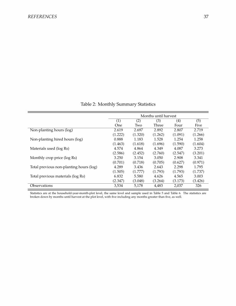
Table 2 presents summary statistics, at the plot level, for five different “months” of the

year: one month prior to harvest, two months prior to harvest, three months prior to

harvest, four months prior to harvest, and five months prior to harvest. The first thing to

note is that total non-planting hours show modest differences by month, with total hours

17

increasing by approximately 30 percent from one month prior to harvest to three months

prior to harvest. Though the overall pattern for hired labor is similar, the magnitude of

the change is much greater for hired labor than for total labor. Total materials used (in

rupees), on the other hand, does not show similar patterns. Rather, materials appear to

be increasing up until one month prior to harvest, at which point they decrease markedly.

Crop prices appear to be increasing as we approach harvest – consistent with the months

just before harvest being the leanest time of the year – other than five months prior to

harvest. However, there are relatively few observations five months prior, so it is difficult

to draw any firm conclusions.

4 Results

4.1 Testing for Separation Using Household Demographics

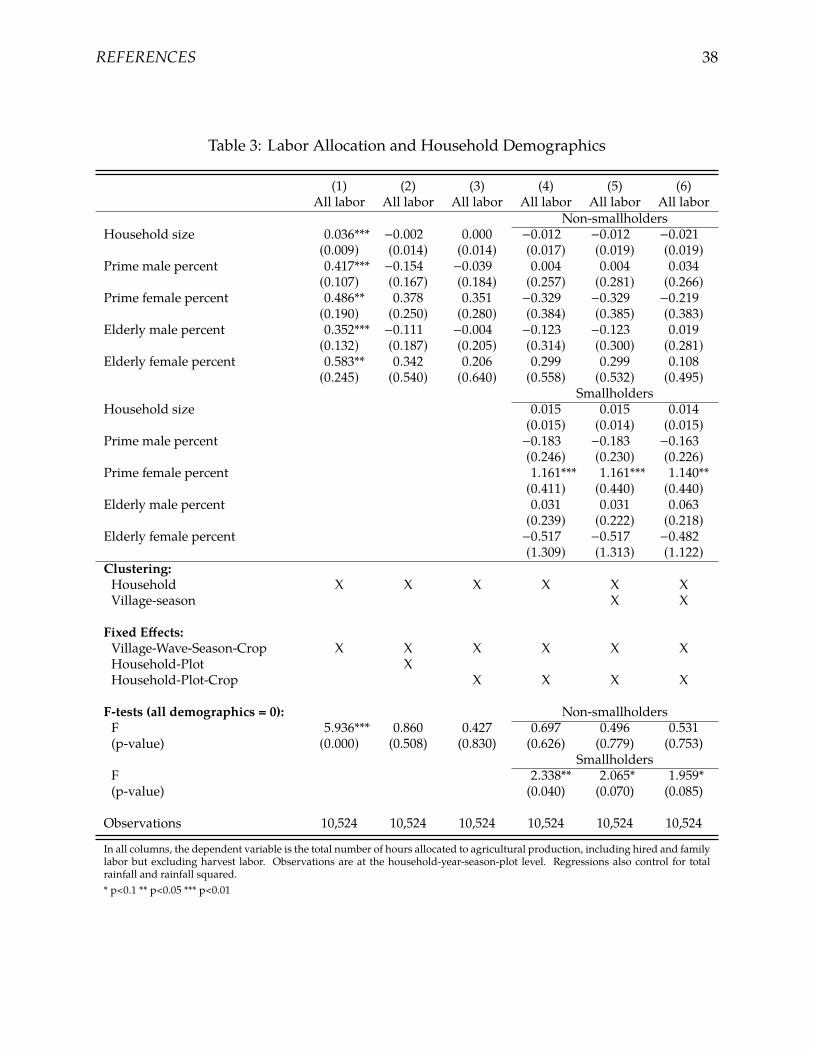
The results begin with the household separation regression in Equation 11. Table 3

presents these results. The first column is a cross-section regression of total plot-level

labor on household demographics. The F-test at the bottom of the table strongly rejects

the null hypothesis for the first column. However, since this is a cross-section regression,

differences in households may be driving the results. Recall that non-smallholder house-

holds tend to be larger than smallholders. Since non-smallholder plots are also larger,

the correlation between household size – though not necessarily household demographic

make-up – and labor demand could be explained by these differences. Consistent with

this, column two – which adds household-plot fixed effects – and column three – which

adds household-plot-crop fixed effects – suggest a much different conclusion. In neither

column do we reject the null hypothesis that all demographic variable coefficients equal

zero.

However, the first three columns assume all households face similar conditions. Since

18

market failures and separation are household-specific, we may be missing the bigger pic-

ture. Columns four through six allow the effects of the demographic variables to differ

across household types.10 It appears that the results do not reject separation for non-

smallholder households, but do reject separation for smallholder households. This is

consistent across the three columns, including when we allow for two-way clustering at

both the household level and the village-season level.11 In other words, it appears that

smallholder households do not act as if markets are complete, as consumption character-

istics are predictors of production decisions. We are unable to reject no correlation for

non-smallholders, however.12

The correlation between demographics and labor demand for smallholders appears

to be driven by prime females. Since the four demographic groups are share variables

and household size is included as a covariate, the share variables are interpreted as

changing the make-up of the household, but not changing the household. The omitted

category is children, so the coefficients are interpreted as increasing each group relative

to (i.e. decreasing) children. For smallholders, apparently having more women and

fewer children leads to an increase in labor demand. One possibility is that women have

more trouble finding outside work than men and, as such, the excess labor is applied to

household production. In this case, to household agricultural production.

4.2 Labor Allocation and Crop Prices

The rest of this paper takes this result at face value and assumes separation holds for

non-smallholders but not for smallholders. Before digging into the key predictions of

differences in price-labor elasticities, I first present evidence that mid-season hours are

10They are estimated in a single regression, however.11Since household-plot fixed effects are included in all columns, area planted is not necessarily a requiredcovariate. Moreover, as shown in Table A3, household size is strongly correlated with area planted onindividual plots. Nonetheless, column six adds area planted and area irrigated as additional covariates.Qualitative conclusions are unchanged.

12Table A4 presents robustness checks of varying demographic definitions. We consistently reject the nullfor smallholders but not for non-smallholders.

19

productive and that there are no obvious cross-plot spillovers due to total labor allocation.

I then show that households respond to changes in crop prices by reallocating labor across

plots based on these price changes.

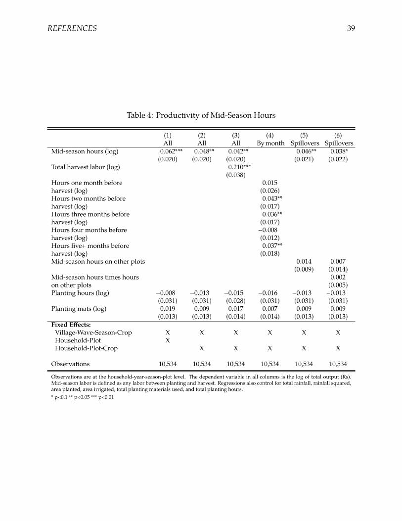
First, Table 4 explores the productivity of mid-season hours – those hours between

planting and harvest. The table presents results from a simple Cobb-Douglas production

function, with log of output, in rupees, as the dependent variable and total mid-season

labor hours (log plus one) as the key independent variable. Additional covariates also

include planting decisions, which are likely correlated with both output and mid-season

hours. Columns one through four show that mid-season hours are significant predictors

of total output at the end of the season. One percent higher mid-season labor hours is

associated with an increase in output of somewhere between 0.04 and 0.06 percent. In

other words, these hours are indeed productive and, as such, farmers may reallocate their

hours in response to changes in expected revenue driven by changes in crop prices.

Since the key prediction this article tests is that market failures lead to a linkage across

plots, we must first rule out spillovers across plots due to other reasons. One possibility is

that there are productivity spillovers due to labor allocation. Perhaps an increase in hours

allocated to plots increases productivity due to bulk purchase discounts, for example.

Columns five and six test this possibility. Column five adds as a covariate total mid-

season hours on other plots. The coefficient is small – less than one-third the size of

the mid-season hours coefficient – and not significantly different from zero. In column

six, I include an additional interaction between mid-season hours on the plot and total

mid-season hours on other plots. Again, there do not appear to be any spillovers related

to mid-season labor allocation, at least not conditional on the other covariates included in

the model.

Next, Table 5 askswhether households reallocate their labor in response toprice changes.

These regressions are at the household-plot-year-month level. The key covariate is now

the price of the crop planted on that plot and, as such, I am no longer able to include

20

village-by-crop-by-year-by-month fixed effects since this is the same level of variation as

crop prices. As such, I move the fixed effect up to the district level instead fo the village

level. As discussed above, I am isolating differences in crop prices across villages within

the same district, conditional on household-plot-crop fixed effects, which should absorb

any permanent differences in crop prices across these same villages. Column one again

presents simple cross-sectional estimates. In the cross-section, there does not appear to

be a correlation between the price of a crop in a specific month and the amount of labor

a household allocates to a plot planted with that crop. Column two adds household-plot

fixed effects and the coefficient increasesmarkedly, by about five times. Column three then

adds planting decisions – labor andmaterials. Although the coefficient is nowmarginally

significant, substantive qualitative conclusions are no different between columns two and

three; there appears to be a slight positive relationship between crop prices and labor

allocation.

Columns one through three include total previous labor and materials allocated to the

plot as well as monthly rainfall totals. However, it seems likely that the effect of these

variables will depend on the month of the year. For example, rainfall during certain

months may be much more important if it increases productivity more than in other

months. As such, column four allows the effects of these covariates to vary by month of

the year. This leads to an increase in the effect of crop price. It appears that households do

indeed reallocate labor in response to changes in crop prices, with an implied elasticity of

approximately 0.3. This elasticity is substantively unchanged if we add household-plot-

crop fixed effects (column five) or the wage rate (column six). We also see an association

between crop price andmaterials, though the coefficient is very imprecisely estimated. As

we will see shortly, these estimates belie important heterogeneity.

Additional specifications are presented in Table A5. For labor, I test an additional

specification adding village-month-crop fixed effects, which removes any village-level

shared variation in the same month of the year for the same crop. This essentially

21

treats seasonal patterns more explicitly, looking at within-village variation in the same

month to the same crop across different years. The second column tests this possibility

even more stringently, by including household-month-crop, instead of village-month-

crop, fixed effects. The coefficients for the labor models actually increase quite markedly,

suggesting even larger price responses. For materials, the household-month-crop fixed

effects specification in column three results in an attenuated coefficient. As such, the labor

results are quite robust, but the materials results are a bit less so.

Recall that when households act as if markets are complete, the relevant labor trade-

off for each plot is between the productivity on that plot and wage employment. If a

household is working both for a wage and on one’s own farm, then when a crop price

increases, the household will shift family labor away from wage work and towards that

crop. On the other hand, if the crop price decreases, the household will shift labor away

from that crop and towards wage employment. Importantly, since households are price

takers, this additional labor allocation to wage employment does not affect the wage.

If markets are not complete, however, this is not the case. For a household that faces a

wage labor constraint, they are not able to shift additional labor towards wage employ-

ment. This means any additional labor allocated to or from a plot must be from/to other

places: leisure, domestic production, or other plots. Unlike with wage employment, this

shift in labor also affects marginal productivity of labor in said tasks. This leads to a

smaller labor reallocation response for these households than for households that are able

to reallocate labor towards or away from wage employment.

Table 6 tests this prediction with four different dependent variables: total mid-season

hours, family mid-season hours, hired mid-season hours, and mid-season materials. Col-

umn one presents the results for all labor. Consistent with economic theory, the elasticity

of labor (re)allocation with respect to the crop price is significantly lower for smallholders

than non-smallholders. For non-smallholders, a one-percent change in the crop price

leads to a change in labor allocation of approximately 0.4 percent. For smallholders, on

22

the other hand, it is just 0.15 percent.

Columns two and three present results for family and hired labor, respectively. While

smallholders and non-smallholders reallocate family labor similarly, non-smallholders

respond to crop price changes with hired labor much more than do smallholders. This is

consistent with a world in which non-smallholder households need to hire in additional

wage labor to meet their labor requirements, but smallholder households have what

amounts to excess labor. Excess labor in this sense refers to smallholders having MRPLs

on their plots lower than themarket wage if theywere to allocate all of their available labor

to own agricultural production. Non-smallholders, on the other hand, would haveMRPLs

higher than the market wage, leading to them hiring additional labor. If true, smallholders

would, on average, hire much less labor than non-smallholders, which is exactly what we

see in the data. Moreover, the average seasonal total planted area per person – across the

crops used in this study – is 2.27 acres per person for non-smallholders but just 0.77 acres

per person for smallholders. We also see a difference in elasticities for materials, though

the estimate for non-smallholders is quite imprecisely estimated.

The appendix presents several different robustness checks. First, Table A6 relaxes iden-

tifying assumptions by including village-year-month-crop fixed effects instead of district-

year-month-crop fixed effects. The level effect of crop price is no longer identified, but

the difference in its effect across household types is. All four specifications yield identical

conclusions. Additionally, column five, including village-year-month-crop-fixed effects,

also adds next month’s crop price and its interaction with smallholder as an additional

covariate. This is included to insure predicted price changes are not driving results. Col-

umn six instead includes district-year-month-crop fixed effects, the same specification as

those in Table 6, as well as the following month’s crop price, for a more apples-to-apples

comparison to the results listed here in the main text. Qualitative conclusions are un-

changed. In other words, it does not appear to be expected seasonal patterns driving the

reallocation of labor.

23

Finally, all specifications in Table 6 include planting variables and the sumof all previous

input choices as covariates. While these are not lagged variables in the traditional sense,

it nonetheless raises some concerns regarding serial correlation and panel data. Table A7

presents results removing all planting and previous input allocation decisions from the

regression. Conclusions are again unchanged.

4.3 Quantifying the Effects of Reallocation on Agricultural Output

If non-smallholder farmers do indeed reallocate labor in response to crop price changes

more than smallholders, this suggests non-smallholders are more able to increase overall

revenue output by responding to unexpected intra-season crop price changes. This section

attempts to quantify this amount. An important caveat is required: these results take

several coefficients at face value and ignore uncertainty in the estimation. As such, the

point estimate should be taken with a grain of salt.

I quantify the effects of labor reallocation in several steps. First, I estimate total mid-

season hours based on the planting and harvest price of the crop, at the household-plot-

year-season level. I estimate this separately for both smallholders and non-smallholders.

Consistent with the main results, non-smallholders appear to respond to harvest price

but smallholders do not. These results are presented in Table A9. I then predict labor

allocation for all households based on each regression, under the assumption that non-

smallholders do not respond to harvest prices. Then, I estimate the effects of mid-season

labor allocation for smallholders and non-smallholders on total output. Using the pre-

dicted labor allocations based on the price change from the first step, I then compute

two separate predicted outputs for each household: one in which they respond to price

signals (like non-smallholders), denoted yNS, and one in which they do not respond to

price signals (like smallholders), denoted yS.

For each household, I then compute the difference between these two, or φdi f f � yNS −

yS. In other words, for every household, φdi f f is the difference in total predicted output

24

basedonwhether they reallocate labor in response toprice changes ornot. Thedistribution

of φdi f f is presented in Figure 2, separately for smallholders and non-smallholders. The

point estimate suggests smallholders could increase their total output by almost 9 percent

if they responded to price changes like non-smallholders. Non-smallholders, on the other

hand, would have total output approximately 16 percent lower if they did not respond

to price changes. Note that this does not include any additional income that might come

from, for example, additionalwage employment if it were available. This estimate pertains

only to a reallocation of labor across plots.

4.4 Accounting for Changes in the Time Use of Household Members

The dataset also collects information onmonthly labor allocation of individual household

members. We can use this information to further explore some aspects of the theory and

perhaps better understand the nature of agricultural production in rural India. To do this,

I look at changes in individual-level time allocation to different productive activities based

on changes in crop prices. One big issue with this is that most households grow more

than one crop. As such, I create a price variable that is a weighted average of all crops

grown by a household, weighted by the percentage of area in a given season allocated to

each crop. In other words, for each household, I look at their total acreage in a season.

I then take the percentage of that total acreage devoted to each individual crop and use

that percentage to weight crop prices. Variation then comes from the changes in these

prices throughout the season. While this is an admittedly imperfect measure, there is no

obvious “price” to use for households that grow more than one crop.

Regressions include district-year-month-crop fixed effects and individual-crop fixed

effects, where crop is defined not as individual crops, but as the exact combination of

crops grown. In other words, identification comes from comparing individuals with the

same combination of crops but with different percentages of land allocated to each crop.

The first set of results are in Table 7. I look at five separate types of activities: own farm

25

days, wage days, other (productive) days, involuntary unemployment days, and non-farm

work days (which are defined as the sum ofwage and other days). I include all individuals

in the dataset and also include age and age squared as covariates. Since there are a lot

of zeros – only 25 percent of individual-month observations have non-zero wage days,

for example – I transform all of the time-use variables using an inverse hyperbolic sine

transformation (Bellemare and Wichman, 2020).13 The first column is own farm days. As

we would expect, we see a positive relationship between monthly (weighted) crop price

and own farm days for both smallholder and non-smallholder households.

Column two presents result for wage labor. There appears to be no relationship between

individual wage employment and crop price. However, this is additional evidence that

many smallholders may face a wage labor constraint; if that constraint is already binding,

then smallholders will not be reallocating any labor to or away from wage employment

unless the MRPL on that household’s plots is only slightly below the market wage, such

that an increase in price would lead them to again equate MRPLs and the market wage.

The negative coefficient is consistent with some households facing such a situation, but

the coefficient is nowhere near significance, so caution is warranted interpreting even the

sign. For non-smallholders, on the other hand, if they need to hire in labor for agricultural

production, we would not expect them to also work on the market. A null effect is

consistent with this.

We see no movement of other days, a relatively ill-defined category. The most interest-

ing results are for involuntary unemployment days. There is a strong negative correlation

between weighted crop price and involuntary unemployment days for smallholders. One

possible interpretation for involuntary unemployment is when an individual searches for

wage employment but fails to find any for a day, resulting in a day of (involuntary) unem-

ployment. While an increase in one’s own crop price(s) should not affect the probability

13Using logs is preferred because it allows for a straightforward elasticity interpretation. As such, in themain results presented above, I use logs as there are many more non-zero observations. Crop price, forexample, is never zero, while mid-season hours has many more non-zero observations. Table A8 presentsthese same time-use results in levels. Qualitative conclusions are unchanged.

26

of finding outside employment conditional on searching, it could affect the probability

an individual searches for outside unemployment. A negative coefficient for smallhold-

ers suggests higher own crop prices makes individuals less likely to search for wage

employment. Again, we see no relationship for non-smallholders, as we would expect.

5 Conclusion

The overall evidence suggests that smallholders and non-smallholders respondmuch dif-

ferently to price changes. These results are especially pertinent in a country like India,

where the government is heavily involved in setting agricultural prices. The Indian gov-

ernment directly affects prices on both the consumption and production sides, through

its public distribution system (PDS) and minimum support price (MSP) policies, respec-

tively. Indirectly, other policies can also impact prices. For example, legislation that

restricts farmers’ sales to only markets within that farmer’s state may artificially depress

prices received by farmers (Chatterjee, 2019).

The policy implications of these findings can be substantial. First and foremost, any

policy changes that affect agricultural prices – like the PDS and MSP – are likely to

have different impacts on agricultural output in different areas. In other words, different

households will respond differently to the same change in price driven by an agricultural

policy. Production may remain relatively constant for a given crop in areas with more

smallholders butmay change significantly in areaswithmore large landholders. Similarly,

the results onnumber of cropsgrownand the increase in elasticity for smallholders suggests

districts with environments more amenable to diverse production may see larger changes

in crop production than districts that are less suitable for diverse production if price of

that crop changes.

Second, but related, changes to crop prices will have larger impacts on non-agricultural

production and production of other crops for different types of households. Theory and

27

results show that in order to increase production of a crop, smallholders must reallocate

labor away from some other type of household production. Non-smallholders, however,

do not. This implies that if, for example, the price of paddy increases, smallholders will

have to decrease labor to production of other crops – if they grow other crops – decreasing

production of those crops. Similarly, they may decrease time spent on other household

production activities, as well. It is not clear from the present results exactly what type of

domestic production decreases, but if less time is spent on human capital accumulation –

time spent with children, for example – then there could be longer term knock-on effects.

This is an interesting avenue for future research.

Third, the overall evidence points to providing off-farm wage employment to small-

holder households as a potential way to increase economy-wide efficiency and improve

the welfare of smallholders. Overallocation of labor to agricultural production leaves

“money on the table” for smallholders. Interestingly, one possible policy intervention in

this area is a public works program, like the Mahatma Gandhi National Rural Employ-

ment Guarantee Scheme (NREGS). NREGS has been found to provide households with

alternative employment opportunities, allowing them to possibly allocate more labor to

riskier productive activities (Gehrke, 2019; Merfeld, 2019). However, it is noteworthy that

the data used in this paper come from after implementation of NREGS. As such, while

it is possible that NREGS “improved” the overallocation of labor seen in smallholders, it

clearly did not completely alleviate the problem.

An important takeaway from these results is that the market context in which a house-

hold operates can drive the household’s behavioral responses to market signals. In other

words, if we were to transplant the smallholder households into an environment in which

they had ample access to off-farm wage labor opportunities, we might see them respond

differently. This argument suggests that it is not necessarily differences in production

technologies, per se, which drive differences in labor supply (and demand) responses. In-

stead, market structure itself can be a defining feature of these responses. This, of course,

28

does not imply that production technologies do not also influence these decisions. How

underlying production characteristics interact with market failures remains an interesting

avenue for future research.

29

References

Barnum, H. N. and Squire, L. (1979). An econometric application of the theory of the

farm-household. Journal of Development Economics, 6(1):79–102.

Bellemare, M. F., Barrett, C. B., and Just, D. R. (2013). The welfare impacts of commodity

price volatility: evidence from rural Ethiopia. American Journal of Agricultural Economics,

95(4):877–899.

Bellemare, M. F. and Wichman, C. J. (2020). Elasticities and the inverse hyperbolic sine

transformation. Oxford Bulletin of Economics and Statistics, 82(1):50–61.

Benjamin, D. (1992). Household composition, labor markets, and labor demand: testing

for separation in agricultural household models. Econometrica, pages 287–322.

Breza, E., Kaur, S., and Shamdasani, Y. (2020). Labor Rationing: A Revealed Preference

Approach from Hiring Shocks.

Brummund, P. and Merfeld, J. (2019). Should farmers farm more? Comparing marginal

products within Malawian households. Working paper.

Chakrabarti, S., Kishore, A., and Roy, D. (2018). Effectiveness of food subsidies in raising

healthy food consumption: public distribution of pulses in India. American Journal of

Agricultural Economics, 100(5):1427–1449.

Chatterjee, S. (2019). Market power and spatial competition in rural india. Working paper.

Chatterjee, S. and Kapur, D. (2016). Understanding Price Variation in Agricultural Com-

modities in India: MSP, Government Procurement, and Agriculture Markets. In India

Policy Forum July, volume 12, page 2016.

Chatterjee, S. and Kapur, D. (2017). Six puzzles in Indian agriculture. In India Policy Forum

2016, volume 17, page 13.

30

Conley, T. G. and Udry, C. R. (2010). Learning about a new technology: Pineapple in

Ghana. American Economic Review, 100(1):35–69.

de Janvry, A., Fafchamps, M., and Sadoulet, E. (1991). Peasant Household Behaviour with

Missing Markets: Some Paradoxes Explained. Economic Journal, 101(409):1400–417.

Dillon, B. and Barrett, C. B. (2017). Agricultural factor markets in Sub-Saharan Africa: An

updated view with formal tests for market failure. Food Policy, 67:64–77.

Dillon, B., Brummund, P., and Mwabu, G. (2019). Asymmetric non-separation and rural

labor markets. Journal of Development Economics, 139:78–96.

Gehrke, E. (2019). An Employment Guarantee as Risk Insurance? Assessing the Effects

of the NREGS on Agricultural Production Decisions. The World Bank Economic Review,

33:413–435.

Jacoby, H. G. (1993). Shadow wages and peasant family labour supply: an econometric

application to the Peruvian Sierra. The Review of Economic Studies, 60(4):903–921.

Jacoby, H. G. and Skoufias, E. (1997). Risk, financial markets, and human capital in a

developing country. The Review of Economic Studies, 64(3):311–335.

Jayachandran, S. (2006). Selling labor low: Wage responses to productivity shocks in

developing countries. Journal of Political Economy, 114(3):538–575.

Jha, R., Bhattacharyya, S., andGaiha, R. (2011). Social safety nets and nutrient deprivation:

An analysis of the National Rural Employment Guarantee Program and the Public

Distribution System in India. Journal of Asian Economics, 22(2):189–201.

Kaur, S. (2019). Nominal wage rigidity in village labor markets. American Economic Review,

forthcoming.

31

Kochar, A. (1999). Smoothing consumption by smoothing income: hours-of-work re-

sponses to idiosyncratic agricultural shocks in rural India. Review of Economics and

Statistics, 81(1):50–61.

LaFave, D., Peet, E., and Thomas, D. (2018). Who behaves as if rural markets are complete?

Colby College Working Paper.

LaFave, D. and Thomas, D. (2016). Farms, families, and markets: New evidence on

completeness of markets in agricultural settings. Econometrica, 84(5):1917–1960.

Meenakshi, J. and Banerji, A. (2005). The unsupportable support price: an analysis

of collusion and government intervention in paddy auction markets in North India.

Journal of Development Economics, 76(2):377–403.

Merfeld, J. D. (2019). Moving up or Just Surviving? Non-Farm Self-Employment in India.

American Journal of Agricultural Economics, forthcoming.

Osborne, T. (2004). Market news in commodity price theory: Application to the Ethiopian

grain market. The Review of Economic Studies, 71(1):133–164.

Rosenzweig, M. R. (1980). Neoclassical theory and the optimizing peasant: An economet-

ric analysis of market family labor supply in a developing country. The Quarterly Journal

of Economics, 94(1):31–55.

Rosenzweig, M. R. and Udry, C. (2014). Rainfall forecasts, weather, and wages over the

agricultural production cycle. American Economic Review, 104(5):278–83.

Rosenzweig, M. R. and Udry, C. (2020). External validity in a stochastic world: Evidence

from low-income countries. The Review of Economic Studies, 87(1):343–381.

Rosenzweig, M. R. and Udry, C. R. (2019). Assessing the Benefits of Long-Run Weather

Forecasting for the Rural Poor: Farmer Investments andWorkerMigration in a Dynamic

Equilibrium Model. National Bureau of Economic Research No. w25894.

32

Sadoulet, E., De Janvry, A., and Benjamin, C. (1998). Household behavior with imperfect

labor markets. Industrial Relations: A Journal of Economy and Society, 37(1):85–108.

Singh, I., Squire, L., and Strauss, J. (1986). The basic model: theory, empirical results, and policy

conclusions, pages 17–47.

Skoufias, E. (1994). Using shadow wages to estimate labor supply of agricultural house-

holds. American Journal of Agricultural Economics, 76(2):215–227.

Strauss, J. (1984). Joint determination of food consumption and production in rural Sierra

Leone: Estimates of a household-firmmodel. Journal of Development Economics, 14(1):77–

103.

Strauss, J. (1986). Does better nutrition raise farmproductivity? Journal of Political Economy,

94(2):297–320.

Suri, T. (2011). Selection and comparative advantage in technology adoption. Econometrica,

79(1):159–209.

Taylor, J. E. and Adelman, I. (2003). Agricultural household models: genesis, evolution,

and extensions. Review of Economics of the Household, 1(1-2):33–58.

Townsend, R. M. (1994). Risk and Insurance in Village India. Econometrica, 62(3):539–591.

Udry, C. (1996). Gender, agricultural production, and the theory of the household. Journal

of Political Economy, 104(5):1010–1046.

Zant,W. (2018). Trains, trade, and transaction costs: Howdoes domestic trade by rail affect

market prices of Malawi agricultural commodities? The World Bank Economic Review,

32(2):334–356.

33

Tables

Figure 1: Agricultural Production and Market Failures

𝐿

$

𝑝$𝑓$(𝐿$; 𝐴$)

𝑝$* 𝑓$(𝐿$; 𝐴$)

𝑤

𝑤

𝐿$ 𝐿$* 𝐿

$

𝑝$𝑓$(𝐿$; 𝐴$)

𝑝$* 𝑓$(𝐿$; 𝐴$)

𝑝,𝜕𝑓,𝜕𝐿,

𝐿$

𝑝,𝜕𝑓,𝜕𝐿,

′

𝐿$*

Panel A: Complete Markets Panel B: Incomplete Markets

34

REFERENCES 35

Figure 2: Effects of Labor Reallocation on Total Output

Smallholder(mean = 0.086)

Non-smallholder(mean = 0.162)

0.5

11.

52

Den

sity

-1 -.5 0 .5 1Difference (assumed reallocation minus no reallocation)

The figure shows the predict difference in output for households that reallocate labor in response to price changes relative tohouseholds that do not reallocate labor in response to price changes.

REFERENCES 36

Table 1: Demography and Plot Summary Statistics

(1) (2) (3) (4)Non-smallholders Smallholders Diff (1-2) p-value

Household size 6.983 5.698 1.285 0.000(3.488) (2.260)

Elderly male percent 0.110 0.102 0.008 0.439(0.145) (0.158)

Elderly female percent 0.027 0.019 0.008 0.092(0.079) (0.065)

Prime male percent 0.493 0.473 0.020 0.287(0.241) (0.240)

Prime female percent 0.146 0.148 −0.001 0.924(0.179) (0.176)

Child percent 0.223 0.258 −0.034 0.025(0.187) (0.199)

Plot area planted (log acres) −0.393 −0.893 0.501 0.000(1.219) (1.148)

Plot area irrigated (percent) 0.581 0.540 0.041 0.218(0.492) (0.497)

Total plot non-harvest labor (log hours) 3.390 3.073 0.317 0.005(1.847) (1.766)

Total area, all plots (log acres) 1.802 0.674 1.128 0.000(1.201) (1.043)

Total non-harvest labor, all plots 3.186 2.165 1.021 0.000(log hours) (2.331) (2.139)Blackgram 0.023 0.020 0.004 0.467

(0.151) (0.140)Chickpea 0.085 0.054 0.031 0.003

(0.278) (0.225)Greengram 0.011 0.006 0.005 0.036

(0.103) (0.078)Groundnut 0.045 0.037 0.008 0.424

(0.207) (0.188)Lentil 0.034 0.026 0.008 0.196

(0.180) (0.158)Maize 0.050 0.073 −0.023 0.025

(0.219) (0.261)Paddy 0.303 0.296 0.007 0.806

(0.460) (0.457)Pigeonpea 0.101 0.103 −0.002 0.908

(0.302) (0.304)Sorghum 0.069 0.120 −0.051 0.001

(0.253) (0.325)Wheat 0.279 0.265 0.014 0.532

(0.448) (0.442)Observations 6,957 3,577

Statistics are at the household-year-season-plot level, the same level and sample used in Table 3. The first column presents meansand standard deviations for non-smallholders, as defined by the survey, while the second column presents the same statistics forsmallholders. The third column presents the difference between (1) and (2) and the fourth column presents the p-value for thatdifference, calculated using a regression and clustering standard errors at the household level.

REFERENCES 37

Table 2: Monthly Summary Statistics

Months until harvest(1) (2) (3) (4) (5)One Two Three Four Five

Non-planting hours (log) 2.619 2.697 2.892 2.807 2.719(1.222) (1.320) (1.262) (1.091) (1.266)

Non-planting hired hours (log) 0.888 1.183 1.528 1.254 1.258(1.463) (1.618) (1.696) (1.590) (1.604)

Materials used (log Rs) 4.574 4.864 4.349 4.087 3.273(2.586) (2.452) (2.760) (2.547) (3.201)

Monthly crop price (log Rs) 3.250 3.154 3.050 2.908 3.341(0.701) (0.718) (0.705) (0.627) (0.971)

Total previous non-planting hours (log) 4.289 3.436 2.643 2.298 1.795(1.505) (1.777) (1.793) (1.793) (1.737)

Total previous materials (log Rs) 6.832 5.580 4.626 4.565 3.003(2.347) (3.048) (3.264) (3.173) (3.426)

Observations 3,534 5,178 4,483 2,037 326

Statistics are at the household-year-month-plot level, the same level and sample used in Table 5 and Table 6. The statistics arebroken down by months until harvest at the plot level, with five including any months greater than five, as well.

REFERENCES 38

Table 3: Labor Allocation and Household Demographics

(1) (2) (3) (4) (5) (6)All labor All labor All labor All labor All labor All labor

Non-smallholdersHousehold size 0.036*** −0.002 0.000 −0.012 −0.012 −0.021

(0.009) (0.014) (0.014) (0.017) (0.019) (0.019)Prime male percent 0.417*** −0.154 −0.039 0.004 0.004 0.034

(0.107) (0.167) (0.184) (0.257) (0.281) (0.266)Prime female percent 0.486** 0.378 0.351 −0.329 −0.329 −0.219

(0.190) (0.250) (0.280) (0.384) (0.385) (0.383)Elderly male percent 0.352*** −0.111 −0.004 −0.123 −0.123 0.019

(0.132) (0.187) (0.205) (0.314) (0.300) (0.281)Elderly female percent 0.583** 0.342 0.206 0.299 0.299 0.108

(0.245) (0.540) (0.640) (0.558) (0.532) (0.495)Smallholders

Household size 0.015 0.015 0.014(0.015) (0.014) (0.015)

Prime male percent −0.183 −0.183 −0.163(0.246) (0.230) (0.226)

Prime female percent 1.161*** 1.161*** 1.140**(0.411) (0.440) (0.440)

Elderly male percent 0.031 0.031 0.063(0.239) (0.222) (0.218)

Elderly female percent −0.517 −0.517 −0.482(1.309) (1.313) (1.122)

Clustering:Household X X X X X XVillage-season X X

Fixed Effects:Village-Wave-Season-Crop X X X X X XHousehold-Plot XHousehold-Plot-Crop X X X X

F-tests (all demographics = 0): Non-smallholdersF 5.936*** 0.860 0.427 0.697 0.496 0.531(p-value) (0.000) (0.508) (0.830) (0.626) (0.779) (0.753)

SmallholdersF 2.338** 2.065* 1.959*(p-value) (0.040) (0.070) (0.085)

Observations 10,524 10,524 10,524 10,524 10,524 10,524

In all columns, the dependent variable is the total number of hours allocated to agricultural production, including hired and familylabor but excluding harvest labor. Observations are at the household-year-season-plot level. Regressions also control for totalrainfall and rainfall squared.* p<0.1 ** p<0.05 *** p<0.01

REFERENCES 39

Table 4: Productivity of Mid-Season Hours

(1) (2) (3) (4) (5) (6)All All All Bymonth Spillovers Spillovers

Mid-season hours (log) 0.062*** 0.048** 0.042** 0.046** 0.038*(0.020) (0.020) (0.020) (0.021) (0.022)

Total harvest labor (log) 0.210***(0.038)

Hours one month before 0.015harvest (log) (0.026)Hours two months before 0.043**harvest (log) (0.017)Hours three months before 0.036**harvest (log) (0.017)Hours four months before −0.008harvest (log) (0.012)Hours five+ months before 0.037**harvest (log) (0.018)Mid-season hours on other plots 0.014 0.007

(0.009) (0.014)Mid-season hours times hours 0.002on other plots (0.005)Planting hours (log) −0.008 −0.013 −0.015 −0.016 −0.013 −0.013

(0.031) (0.031) (0.028) (0.031) (0.031) (0.031)Planting mats (log) 0.019 0.009 0.017 0.007 0.009 0.009

(0.013) (0.013) (0.014) (0.014) (0.013) (0.013)Fixed Effects:Village-Wave-Season-Crop X X X X X XHousehold-Plot XHousehold-Plot-Crop X X X X X

Observations 10,534 10,534 10,534 10,534 10,534 10,534

Observations are at the household-year-season-plot level. The dependent variable in all columns is the log of total output (Rs).Mid-season labor is defined as any labor between planting and harvest. Regressions also control for total rainfall, rainfall squared,area planted, area irrigated, total planting materials used, and total planting hours.* p<0.1 ** p<0.05 *** p<0.01

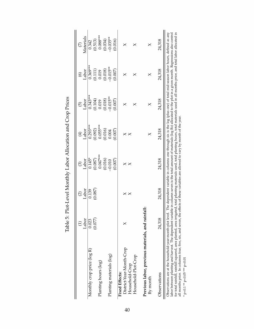
Table5:

Plot-Level

Mon

thly

Labo

rAllo

catio

nan

dCropPrices

(1)

(2)

(3)

(4)

(5)

(6)

(7)

Labo

rLa

bor

Labo

rLa

bor

Labo

rLa

bor

Materials

Mon

thly

crop

price(lo

gR)

0.02

30.

139

0.14

5*0.

293***

0.34

3***

0.36

9***

0.34

2(0.0

77)

(0.0

87)

(0.0

87)

(0.0

92)

(0.1

04)

(0.1

11)

(0.5

13)

Plan

tingho

urs(

log)

0.04

7***

0.05

5***

0.01

90.

019

0.08

8***

(0.0

16)

(0.0

16)

(0.0

18)

(0.0

18)

(0.0

34)

Plan

tingmaterials(lo

g)−0.0

100.

004

−0.0

15**

−0.0

15**

−0.0

35**

(0.0

07)

(0.0

07)

(0.0

07)

(0.0

07)

(0.0

16)

FixedEff

ects:

District-Y

ear-Mon

th-C

rop

XX

XX

XX

XHou

seho

ld-C

rop

XX

XHou

seho

ld-Plot-C

rop

XX

X

Prev

ious

labo

r,prev

ious

materials,and

rainfall:

Bymon

thX

XX

X

Observa

tions

24,318

24,318

24,318

24,318

24,318

24,318

24,318

Observa

tions

areat

theho

useh

old-ye

ar-m

onth-plotlevel.Th

ede

pend

entv

ariablein

columns

onethroug

hsixis

thelog(pluson

e)of

totalm

id-seasonlabo

rho

urs,de

fined

asan

ylabo

rbetweenplan

tingan

dha

rvest.Th

ede

pend

entv

ariablein

columnseve

nisthetotala

mou

ntof

materials(lo

gRs

)allo

catedto

theplot

inagive

nmon

th.R

egressions

also

control

fortotal

rainfall,

rainfallsqua

red,

area

plan

ted,

area

irrigated

,total

plan

tingmaterialsus

ed,total

plan

tingho

urs,totalm

aterialsus

edin

allm

onthsprior,an

dtotallab

orallocatedin

allm

onthsp

rior.In

columns

four,fi

ve,six,a

ndseve

n,theeff

ects

oftheseva

riables

areallowed

tova

ryby

mon

thof

theye

ar.

*p<0

.1**

p<0.05

***p

<0.01

40

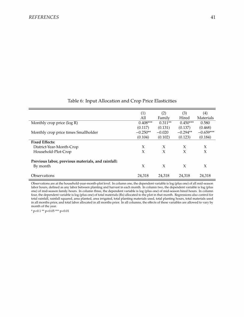
REFERENCES 41

Table 6: Input Allocation and Crop Price Elasticities

(1) (2) (3) (4)All Family Hired Materials

Monthly crop price (log R) 0.408*** 0.311** 0.450*** 0.580(0.117) (0.131) (0.137) (0.468)

Monthly crop price times Smallholder −0.250** −0.020 −0.294** −0.659***(0.104) (0.102) (0.123) (0.184)

Fixed Effects:District-Year-Month-Crop X X X XHousehold-Plot-Crop X X X X

Previous labor, previous materials, and rainfall:By month X X X X

Observations 24,318 24,318 24,318 24,318

Observations are at the household-year-month-plot level. In column one, the dependent variable is log (plus one) of all mid-seasonlabor hours, defined as any labor between planting and harvest in each month. In column two, the dependent variable is log (plusone) of mid-season family hours. In column three, the dependent variable is log (plus one) of mid-season hired hours. In columnfour, the dependent variable is log (plus one) of total materials (Rs) allocated to the plot in that month. Regressions also control fortotal rainfall, rainfall squared, area planted, area irrigated, total planting materials used, total planting hours, total materials usedin all months prior, and total labor allocated in all months prior. In all columns, the effects of these variables are allowed to vary bymonth of the year.* p<0.1 ** p<0.05 *** p<0.01

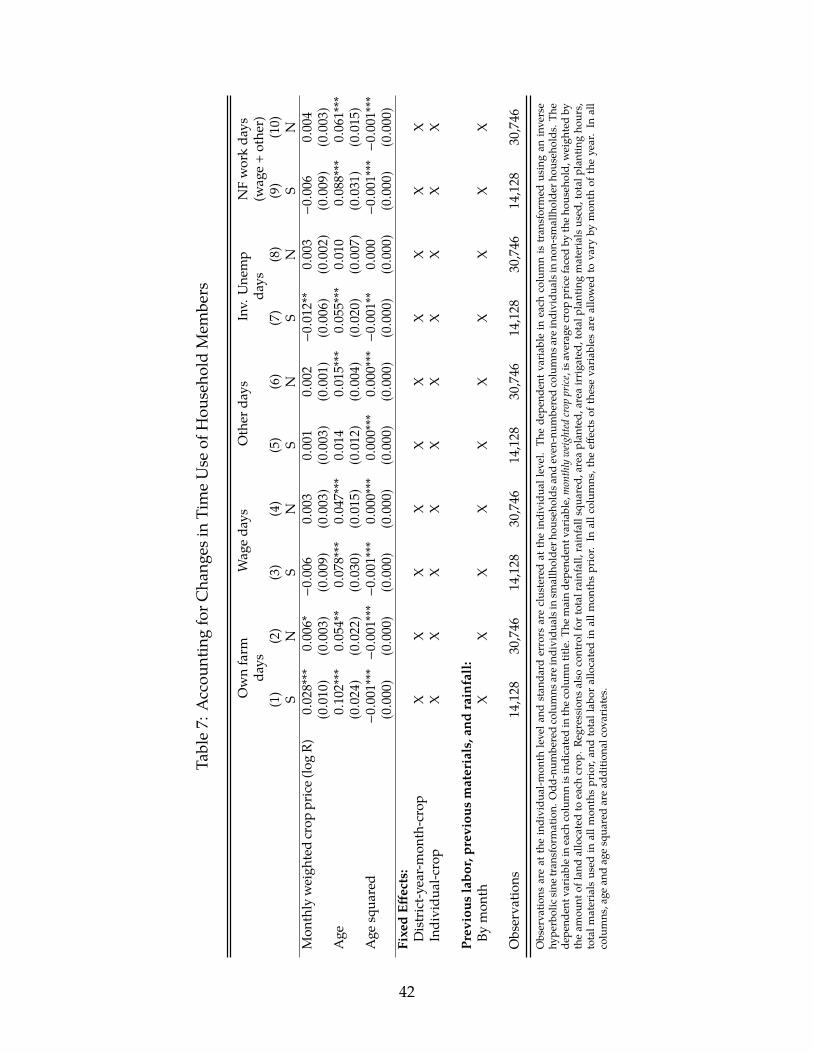
Table7:

Accou

ntingforC

hang

esin

TimeUse

ofHou

seho

ldMem

bers

Ownfarm

Wag

eda

ysOther

days

Inv.

Une

mp

NFworkda

ysda

ysda

ys(w

age+othe

r)(1)

(2)

(3)

(4)

(5)

(6)

(7)

(8)

(9)

(10)

SN

SN

SN

SN

SN

Mon

thly

weigh

tedcrop

price(

logR)

0.02

8***

0.00

6*−0.0

060.

003

0.00

10.

002

−0.0

12**

0.00

3−0.0

060.

004

(0.0

10)

(0.0

03)

(0.0

09)

(0.0

03)

(0.0

03)

(0.0

01)

(0.0

06)

(0.0

02)

(0.0

09)

(0.0

03)

Age

0.10

2***

0.05

4**

0.07

8***

0.04

7***

0.01

40.

015***

0.05

5***

0.01

00.

088***

0.06

1***

(0.0

24)

(0.0

22)

(0.0

30)

(0.0

15)

(0.0

12)

(0.0

04)

(0.0

20)

(0.0

07)

(0.0

31)

(0.0

15)

Age

squa

red

−0.0

01***−0.0

01***−0.0

01***

0.00

0***

0.00

0***

0.00

0***−0.0

01**

0.00

0−0.0

01***−0.0

01***

(0.0

00)

(0.0

00)

(0.0

00)

(0.0

00)

(0.0

00)

(0.0

00)

(0.0

00)

(0.0

00)

(0.0

00)

(0.0

00)

FixedEff

ects:

District-y

ear-mon

th-crop

XX

XX

XX

XX

XX

Individu

al-crop

XX

XX

XX

XX

XX

Prev

ious

labo

r,prev

ious

materials,and

rainfall:

Bymon

thX

XX

XX

XX

XX

X

Observa

tions

14,128

30,746

14,128

30,746

14,128

30,746

14,128

30,746

14,128

30,746

Observa

tions

areat

theindividu

al-m

onth

leve

land

stan

dard

errors

areclus

teredat

theindividu

alleve

l.Th

ede

pend

entv

ariablein

each

columnis

tran

sformed

usingan

inve

rse

hype

rbolicsine

tran

sformation.

Odd

-num

beredcolumns

areind

ividua

lsin

smallholde

rhou

seho

ldsa

ndeven

-num

beredcolumns

areind

ividua

lsin

non-sm

allholde

rhou

seho

lds.

The

depe

nden

tvariablein

each

columnisindicatedin

thecolumntitle.T

hemainde

pend

entv

ariable,mon

thlyweig

hted

crop

price

,isa

verage

crop

pricefacedby

theho

useh

old,

weigh

tedby

theam

ount

ofland

allocatedto

each

crop

.Reg

ressions

also

controlfor

totalrainfall,rainfallsqua

red,

area

plan

ted,

area

irrigated

,total

plan

tingmaterialsus

ed,total

plan

tingho

urs,

totalm

aterials

used

inallm

onthsprior,an

dtotallab

orallocatedin

allm

onthsprior.

Inallc

olum

ns,the

effects

oftheseva

riables

areallowed

tova

ryby

mon

thof

theye

ar.In

all

columns

,age

andag

esqua

redaread

ditio

nalcov

ariates.

42

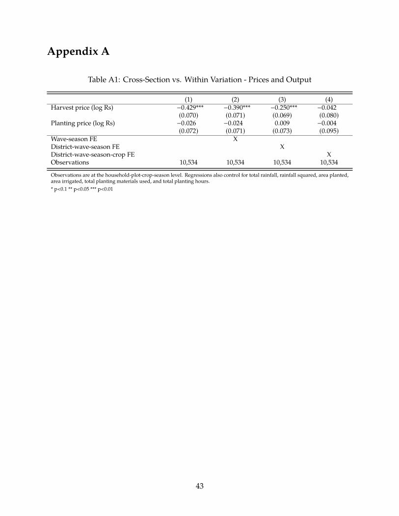
Appendix A

Table A1: Cross-Section vs. Within Variation - Prices and Output

(1) (2) (3) (4)Harvest price (log Rs) −0.429*** −0.390*** −0.250*** −0.042

(0.070) (0.071) (0.069) (0.080)Planting price (log Rs) −0.026 −0.024 0.009 −0.004

(0.072) (0.071) (0.073) (0.095)Wave-season FE XDistrict-wave-season FE XDistrict-wave-season-crop FE XObservations 10,534 10,534 10,534 10,534

Observations are at the household-plot-crop-season level. Regressions also control for total rainfall, rainfall squared, area planted,area irrigated, total planting materials used, and total planting hours.* p<0.1 ** p<0.05 *** p<0.01

43

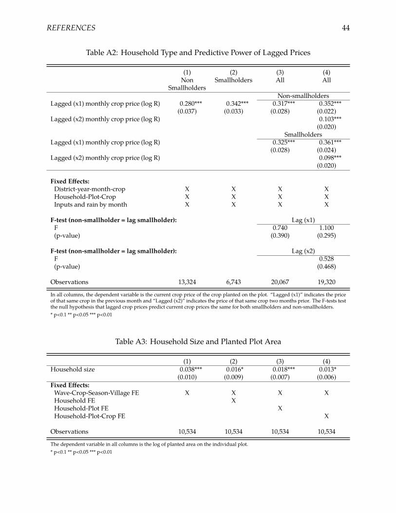
REFERENCES 44

Table A2: Household Type and Predictive Power of Lagged Prices

(1) (2) (3) (4)Non Smallholders All All

SmallholdersNon-smallholders

Lagged (x1) monthly crop price (log R) 0.280*** 0.342*** 0.317*** 0.352***(0.037) (0.033) (0.028) (0.022)

Lagged (x2) monthly crop price (log R) 0.103***(0.020)

SmallholdersLagged (x1) monthly crop price (log R) 0.325*** 0.361***

(0.028) (0.024)Lagged (x2) monthly crop price (log R) 0.098***

(0.020)

Fixed Effects:District-year-month-crop X X X XHousehold-Plot-Crop X X X XInputs and rain by month X X X X

F-test (non-smallholder = lag smallholder): Lag (x1)F 0.740 1.100(p-value) (0.390) (0.295)

F-test (non-smallholder = lag smallholder): Lag (x2)F 0.528(p-value) (0.468)

Observations 13,324 6,743 20,067 19,320

In all columns, the dependent variable is the current crop price of the crop planted on the plot. “Lagged (x1)” indicates the priceof that same crop in the previous month and “Lagged (x2)” indicates the price of that same crop two months prior. The F-tests testthe null hypothesis that lagged crop prices predict current crop prices the same for both smallholders and non-smallholders.* p<0.1 ** p<0.05 *** p<0.01

Table A3: Household Size and Planted Plot Area

(1) (2) (3) (4)Household size 0.038*** 0.016* 0.018*** 0.013*

(0.010) (0.009) (0.007) (0.006)Fixed Effects:Wave-Crop-Season-Village FE X X X XHousehold FE XHousehold-Plot FE XHousehold-Plot-Crop FE X

Observations 10,534 10,534 10,534 10,534

The dependent variable in all columns is the log of planted area on the individual plot.* p<0.1 ** p<0.05 *** p<0.01

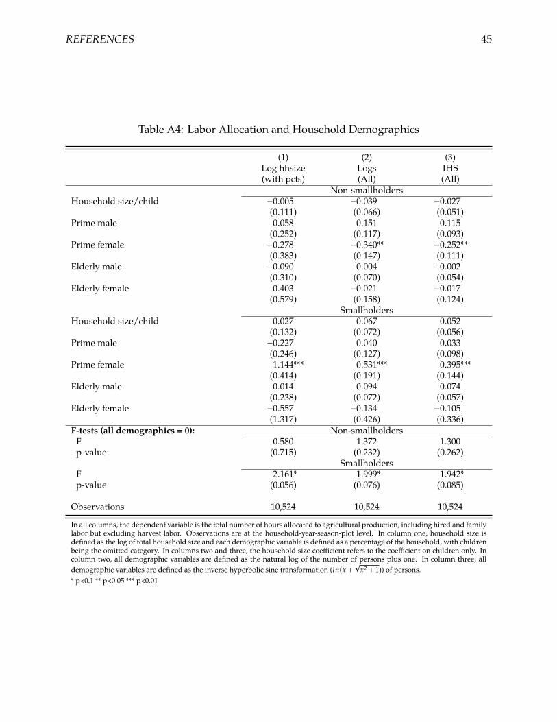
REFERENCES 45

Table A4: Labor Allocation and Household Demographics

(1) (2) (3)Log hhsize Logs IHS(with pcts) (All) (All)

Non-smallholdersHousehold size/child −0.005 −0.039 −0.027

(0.111) (0.066) (0.051)Prime male 0.058 0.151 0.115

(0.252) (0.117) (0.093)Prime female −0.278 −0.340** −0.252**

(0.383) (0.147) (0.111)Elderly male −0.090 −0.004 −0.002

(0.310) (0.070) (0.054)Elderly female 0.403 −0.021 −0.017

(0.579) (0.158) (0.124)Smallholders

Household size/child 0.027 0.067 0.052(0.132) (0.072) (0.056)

Prime male −0.227 0.040 0.033(0.246) (0.127) (0.098)

Prime female 1.144*** 0.531*** 0.395***(0.414) (0.191) (0.144)

Elderly male 0.014 0.094 0.074(0.238) (0.072) (0.057)

Elderly female −0.557 −0.134 −0.105(1.317) (0.426) (0.336)

F-tests (all demographics = 0): Non-smallholdersF 0.580 1.372 1.300p-value (0.715) (0.232) (0.262)

SmallholdersF 2.161* 1.999* 1.942*p-value (0.056) (0.076) (0.085)

Observations 10,524 10,524 10,524

In all columns, the dependent variable is the total number of hours allocated to agricultural production, including hired and familylabor but excluding harvest labor. Observations are at the household-year-season-plot level. In column one, household size isdefined as the log of total household size and each demographic variable is defined as a percentage of the household, with childrenbeing the omitted category. In columns two and three, the household size coefficient refers to the coefficient on children only. Incolumn two, all demographic variables are defined as the natural log of the number of persons plus one. In column three, alldemographic variables are defined as the inverse hyperbolic sine transformation (ln(x +

√x2 + 1)) of persons.

* p<0.1 ** p<0.05 *** p<0.01

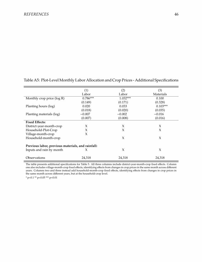
REFERENCES 46

TableA5: Plot-LevelMonthly LaborAllocation andCropPrices -Additional Specifications

(1) (2) (3)Labor Labor Materials

Monthly crop price (log R) 0.786*** 1.032*** 0.100(0.149) (0.171) (0.328)

Planting hours (log) 0.020 0.033 0.103***(0.018) (0.020) (0.035)

Planting materials (log) −0.007 −0.002 −0.016(0.007) (0.008) (0.016)

Fixed Effects:District-year-month-crop X X XHousehold-Plot-Crop X X XVillage-month-crop XHousehold-month-crop X X

Previous labor, previous materials, and rainfall:Inputs and rain by month X X X

Observations 24,318 24,318 24,318

The table presents additional specifications for Table 5. All three columns include district-year-month-crop fixed effects. Columnone also includes village-month-crop fixed effects, identifying effects from changes in crop prices in the samemonth across differentyears. Columns two and three instead add household-month-crop fixed effects, identifying effects from changes in crop prices inthe same month across different years, but at the household-crop level.* p<0.1 ** p<0.05 *** p<0.01

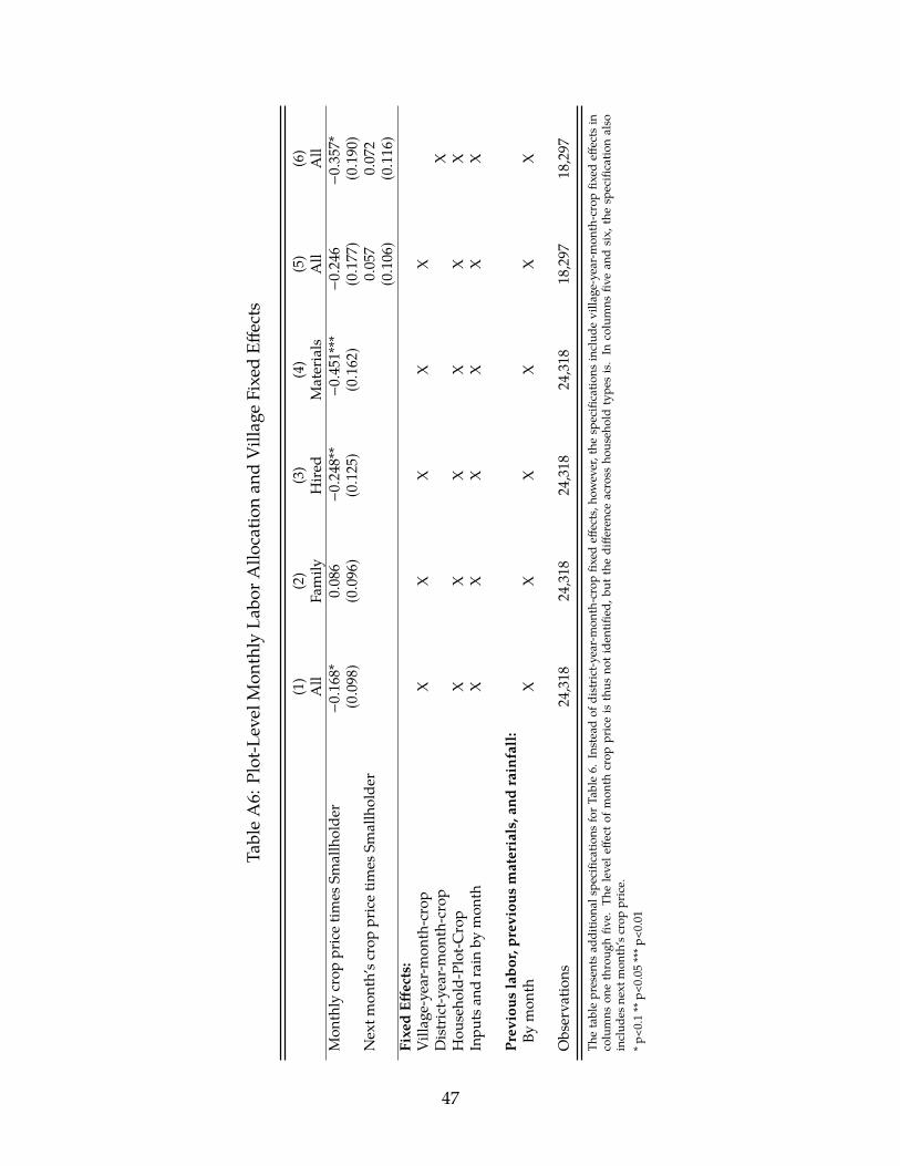
TableA6:

Plot-Level

Mon

thly

Labo

rAllo

catio

nan

dVillag

eFixedEff

ects

(1)

(2)

(3)

(4)

(5)

(6)

All

Family

Hire

dMaterials

All

All

Mon

thly

crop

pricetim

esSm

allholde

r−0.1

68*

0.08

6−0.2

48**

−0.4

51***

−0.2

46−0.3

57*

(0.0

98)

(0.0

96)

(0.1

25)

(0.1

62)

(0.1

77)

(0.1

90)

Nextm

onth’scrop

pricetim

esSm

allholde

r0.

057

0.07

2(0.1

06)

(0.1

16)

FixedEff

ects:

Villag

e-year-m

onth-crop

XX

XX

XDistrict-y

ear-mon

th-crop

XHou

seho

ld-Plot-C

rop

XX

XX

XX

Inpu

tsan

drain

bymon

thX

XX

XX

X

Prev

ious

labo

r,prev

ious

materials,and

rainfall:

Bymon

thX

XX

XX

X

Observa

tions

24,318

24,318

24,318

24,318

18,297

18,297

Thetablepresen

tsad

ditio

nals

pecific

ations

forT

able

6.Insteadof

distric

t-year-mon

th-cropfix

edeff

ects,h

owever,the

specificatio

nsinclud

evilla

ge-year-mon

th-cropfix

edeff

ects

incolumns

onethroug

hfiv

e.Th

eleve

leffe

ctof

mon

thcrop

priceis

thus

notide

ntified

,but

thediffe

renc

eacross

hous

eholdtype

sis.In

columns

fivean

dsix,

thesp

ecificatio

nalso

includ

esne

xtmon

th’scrop

price.

*p<0

.1**

p<0.05

***p

<0.01

47

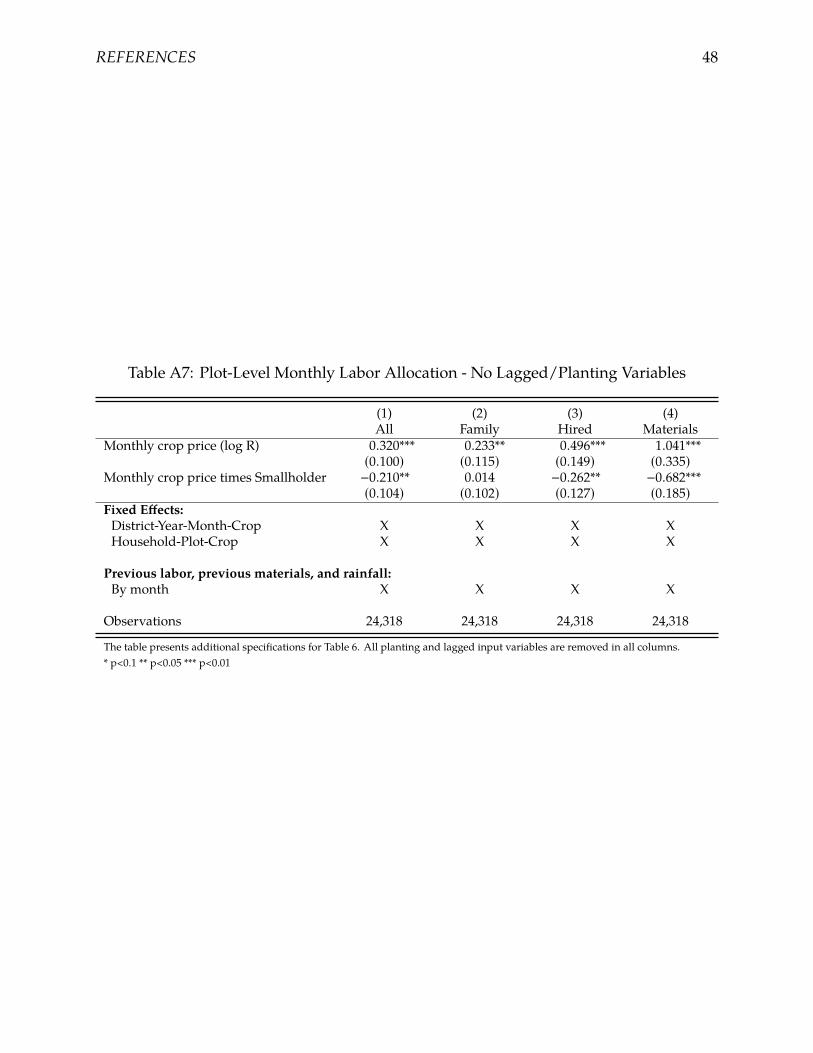
REFERENCES 48

Table A7: Plot-Level Monthly Labor Allocation - No Lagged/Planting Variables

(1) (2) (3) (4)All Family Hired Materials

Monthly crop price (log R) 0.320*** 0.233** 0.496*** 1.041***(0.100) (0.115) (0.149) (0.335)

Monthly crop price times Smallholder −0.210** 0.014 −0.262** −0.682***(0.104) (0.102) (0.127) (0.185)

Fixed Effects:District-Year-Month-Crop X X X XHousehold-Plot-Crop X X X X

Previous labor, previous materials, and rainfall:By month X X X X

Observations 24,318 24,318 24,318 24,318

The table presents additional specifications for Table 6. All planting and lagged input variables are removed in all columns.* p<0.1 ** p<0.05 *** p<0.01

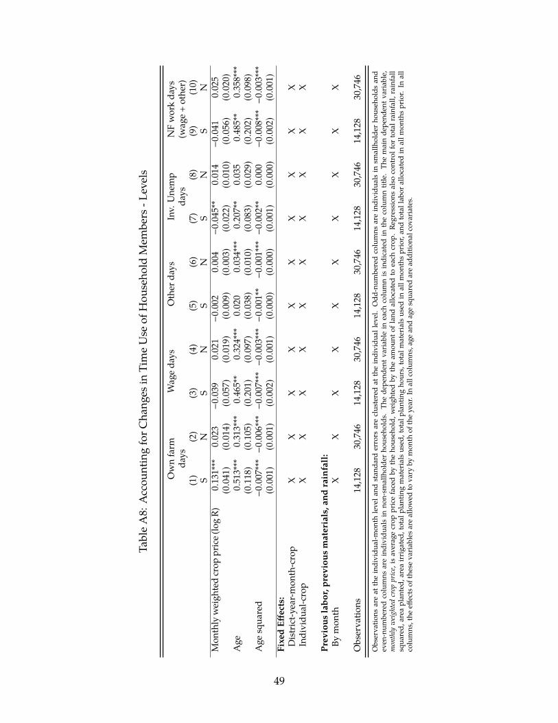
TableA8:

Accou

ntingforC

hang

esin

TimeUse

ofHou

seho

ldMem

bers

-Levels

Ownfarm

Wag

eda

ysOther

days

Inv.

Une

mp

NFworkda

ysda

ysda

ys(w

age+othe

r)(1)

(2)

(3)

(4)

(5)

(6)

(7)

(8)

(9)

(10)

SN

SN

SN

SN

SN

Mon

thly

weigh

tedcrop

price(

logR)

0.13

1***

0.02

3−0.0

390.

021

−0.0

020.

004

−0.0

45**

0.01

4−0.0

410.

025

(0.0

41)

(0.0

14)

(0.0

57)

(0.0

19)

(0.0

09)

(0.0

03)

(0.0

22)

(0.0

10)

(0.0

56)

(0.0

20)

Age

0.51

3***

0.31

3***

0.46

5**

0.32

4***

0.02

00.

034***

0.20

7**

0.03

50.

485**

0.35

8***

(0.1

18)

(0.1

05)

(0.2

01)

(0.0

97)

(0.0

38)

(0.0

10)

(0.0

83)

(0.0

29)

(0.2

02)

(0.0

98)

Age

squa

red

−0.0

07***−0.0

06***−0.0

07***−0.0

03***−0.0

01**−0.0

01***−0.0

02**

0.00

0−0.0

08***−0.0

03***

(0.0

01)

(0.0

01)

(0.0

02)

(0.0

01)

(0.0

00)

(0.0

00)

(0.0

01)

(0.0

00)

(0.0

02)

(0.0

01)

FixedEff

ects:

District-y

ear-mon

th-crop

XX

XX

XX

XX

XX

Individu

al-crop

XX

XX

XX

XX

XX

Prev

ious

labo

r,prev

ious

materials,and

rainfall:

Bymon

thX

XX

XX

XX

XX

X

Observa

tions

14,128

30,746

14,128

30,746

14,128

30,746

14,128

30,746

14,128

30,746

Observa

tions

areat

theindividu

al-m

onth

leve

land

stan

dard

errors

areclus

teredat

theindividu

alleve

l.Odd

-num

beredcolumns

areindividu

alsin

smallholde

rho

useh

olds

and

even

-num

beredcolumns

areindividu

alsin

non-sm

allholde

rho

useh

olds

.Th

ede

pend

entv

ariablein

each

columnis

indicatedin

thecolumntitle.Th

emainde

pend

entv

ariable,

mon

thly

weig

hted

crop

price,is

averag

ecrop

pricefacedby

theho

useh

old,

weigh

tedby

theam

ount

ofland

allocatedto

each

crop

.Re

gression

salso

controlfor

totalrainfall,rainfall

squa

red,

area

plan

ted,

area

irrigated

,total

plan

tingmaterials

used

,total

plan

tingho

urs,totalm

aterials

used

inallm

onthsprior,an

dtotallab

orallocatedin

allm

onthsprior.

Inall

columns

,the

effects

oftheseva

riables

areallowed

tova

ryby

mon

thof

theye

ar.Inallcolum

ns,a

gean

dag

esqua

redaread

ditio

nalcov

ariates.

49

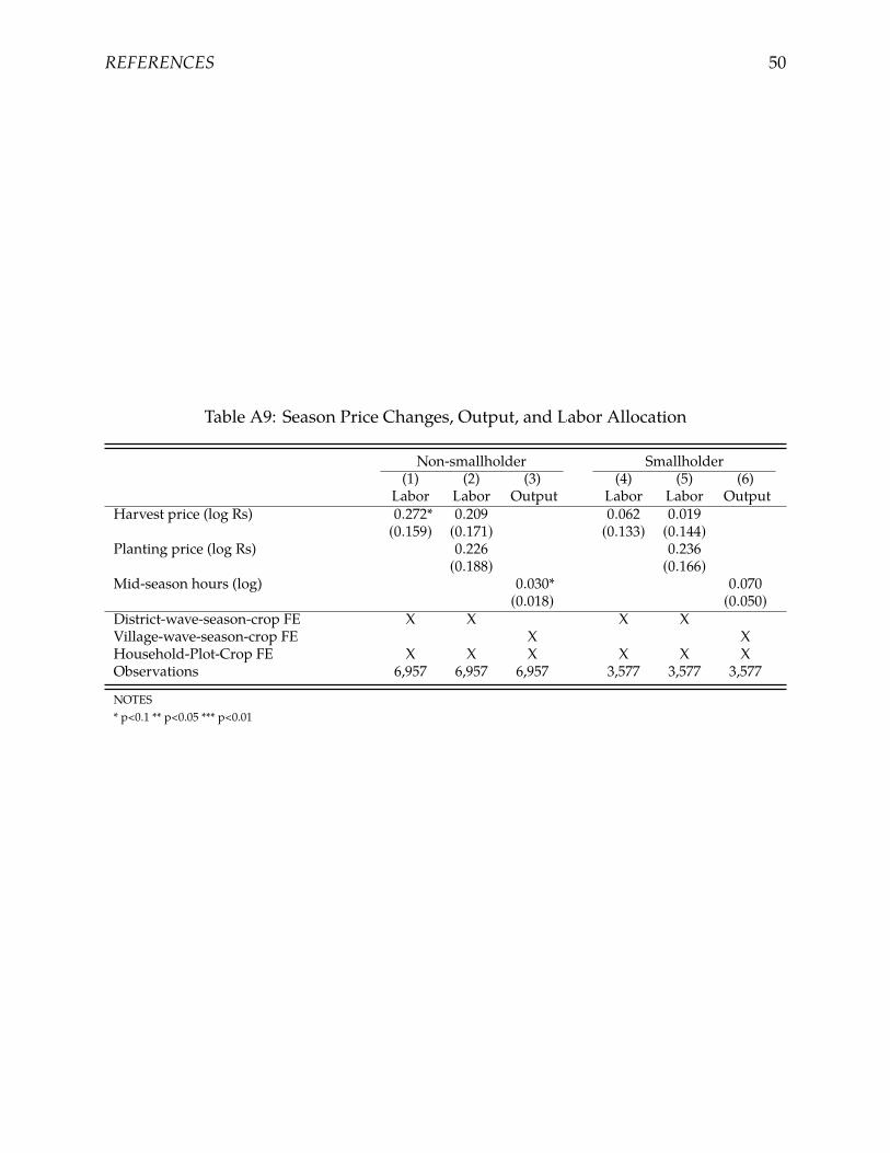
REFERENCES 50

Table A9: Season Price Changes, Output, and Labor Allocation

Non-smallholder Smallholder(1) (2) (3) (4) (5) (6)

Labor Labor Output Labor Labor OutputHarvest price (log Rs) 0.272* 0.209 0.062 0.019

(0.159) (0.171) (0.133) (0.144)Planting price (log Rs) 0.226 0.236

(0.188) (0.166)Mid-season hours (log) 0.030* 0.070

(0.018) (0.050)District-wave-season-crop FE X X X XVillage-wave-season-crop FE X XHousehold-Plot-Crop FE X X X X X XObservations 6,957 6,957 6,957 3,577 3,577 3,577

NOTES* p<0.1 ** p<0.05 *** p<0.01