Embed Size (px)
Citation preview
ANNALS OF PHYSICS 82, 501-534 (1974)
Simplified Bethe-Salpeter Equation for Positronium*
GORDON FELDMAN, THOMAS FULTON, AND JOHN TOWNSEND
Department of Physics, The Johns Hopkins University, Baltimore, Maryland 21218
Received March 16, 1973
The Bethe-Salpeter equation for a fermion-antifermion system, coupled by photons, is considered in the Feynman gauge. The kernel is that resulting from exchange of a single photon. The usual reduction of the sixteen B-S spinor amplitudes in terms of tensors leads to 16 coupled integro-differential equations. By straightforward application of charge conjugation-, parity-, and Lorentz-invariance, the system of coupled equations is reduced to ones involving no more than eight and as few as three scalar structure functions for the various parity, charge conjugation, and total angular momentum states. The results hold for arbitrary coupling strength. As a check of the equations obtained, a perturbation theory is carried out for the Coulomb interaction. It leads to effective potentials in agreement with those obtained previously to order mor4 for positronium.
1. INTRODUCTION
The Bethe-Salpeter equation for a fermion and antifermion of spin + has received periodic attention since its postulation twenty-one years ago [l]. It is therefore remarkable that, except for the strong-coupling bound state where the total mass of the bound state [2-51 is zero, no really satisfactory solutions exist for this system. Although perturbation theories developed to calculate the energy levels of positronium [6,7] to order ma5 (and to order ma6 In 01 for the ground- state singlet-triplet splitting [S]) have been remarkably successful in obtaining numerical results, they have a rather unsatisfactory ad hoc character. Moreover, the techniques become unmanageablely complicated if an attempt is made to extend the calculations to the next higher order, mo!. Experimental accuracy has recently become sufficiently great to detect contributions to this order [9]. Thus, both fundamental considerations of principle as well as practical demands dictate a reexamination of the problem.
In this paper we present what is, hopefully, a first step in such a program. We consider the fermion-antifermion problem with the B-S kernel involving the exchange of a single photon, initially in the Feynman gauge. Other interactions and coupling strengths could also be considered, of course, but we concentrate
* Supported in part by the National Science Foundation.
501 Copyright 0 1974 by Academic Press, Inc. All rights of reproduction in any form reserved.

502 FELDMAN, FULTON AND TOWNSEND
our attention on the positronium problem. The system of equations we obtain could perhaps form the basis of a more systematic perturbation theory.
Our starting point in the next section is the set of coupled equations for the 16 tensor amplitudes S, P, I’, , A, , and Tuy , first obtained by Kummer [4] by carrying out a reduction of the 16 component bi-spinor wave function quip . The system of equations is shown in Ref. [4] to decouple, in the limit when the total mass of the system vanishes, into a separate equation for S, ten coupled equations for the Vu , Tuy system, and five for the P, A, system for both vector and pseudo- vector coupling in the Feynman “gauge.“l We show that, in fact, it is possible to decouple the equations for the case of arbitrary coupling strength (including the relevant electromagnetic coupling), using simple arguments based on the fact that rest mass, total angular momentum, parity, and charge conjugation are simul- taneous observables for our system. We can define scalar structure functions and derive fully covariant equations coupling as few as three (for the case of Y$, in the Feynman gauge), and never more than eight, of these structure functions in any gauge. Our results are analogous to those obtained for the Dirac equation con- taining the Coulomb interaction, for which two independent structure functions are adequate to describe the problem, even though the original equation couples four spinor components.
In Section 3 we apply our equations in the nonrelativistic limit of the weak- binding case for the Coulomb interaction which is, of course, instantaneous (i.e., does not contain relative time). In all cases involving an instantaneous interaction we can solve for the “instantaneous” wave function. This leads immediately to equations involving two structure functions for the lJJ and “JJ systems and to four structure functions for the 3(J f l)J system. Perturbation theory is applied to obtain the effective potentials correct to order ma4, which agree with those obtained by others [lO-121.
2. COVARIANT REDUCTION OF COUPLED EQUATIONS
We first outline the relevant sections of Ref. [4], adopting the notation used there wherever convenient. The fermion-antifermion wave function can be written in momentum space in terms of the single-particle operators # and $ as
am = j d4x ei?‘a2 (0 I 7IN49 $(--x/2)1 IB) YS
s (2.1)
= d4x eiP*xeip.x (0 j T[$(x,) $(x9] I B) y5 ,
1 The concept of “gauge” is meant to denote the character of the interaction only, since it is not applicable for massive bosons or, in the strong-coupling limit, to the single meson exchange kernel.

BETHE-SALPETER EQUATION FOR POSITRONIUM 503
where P is the total four-momentum of the bound state B with X its conjugate coordinate andp is the relative momentum with x its conjugate coordinate:
p = Pl + Pz 3 x = Xl + x2
2 ’
p = PI - P2 -3 2
x = x1 - x2 . (2.2)
Thus, in writing Eq. (2.1), we have made use of translational invariance to factor out the overall center-of-mass coordinate dependence from the fermion-anti- fermion amplitude2 (0 ] T[#(x,) $(x2)11 B).
We will take the center-of-mass frame at rest and from now on will suppress the subscript P(y, -+ y). In order to make comparison with Ref. [4] easy, we write our equation in the Euclidean metric.3 We set
P = (2ip, 0), p = 1 - B/2 (2.3) and define
b = G-G 01, (2.3)
where B is the binding energy, and we have taken the free particle rest mass m to be unity. The B-S equation with an interaction kernel involving one-photon exchange (the ladder approximation) in the Feynman gauge then becomes
with (P’ + ibr + 1) 90 - iP - 1) = y&yu, (2.4)
A=-&. (2.5)
The y’s used in Ref. [4] are defined in Appendix A. The tensor decomposition of v is given by4
v = S + iy6P + iy,V, + iy,y,A,, + o,,T,, . (2.6)
To, is an antisymmetric tensor in the above equation. Since p and p. are real, it can be shown [4] that y is a Hermitian matrix, and, therefore, the tensor structure
2 Following the notation of Ref. [4], we have introduced a yj in the definition of the B-S wave function of Eq. (2.1). As we will see, this has the effect of making the structure function S rather than the structure function P of Eq. (2.6) appear in the 5, state.
a Our subsequent arguments in this section are not based on the choice of the Euclidean rather than the Minkowski metric.
4 The functions P, V, and A, of Eqs. (1.13) of Ref. [4] are redefined through multiplication by a factor of i.

504 FELDMAN, FULTON AND TOWNSEND
functions are real. The B-S equation in terms of these structure functions is given by5
-(p” + /.L~ + 1) S - 2b,V, - 4p,,b,T,,, = -4IS, (2.7)
(p” + /t2 - 1) P - 2p,A, - 4p,b,T,,, = 4IP, (2.8)
--2b,,S + (P” + p2 - 1) V, - 2(p,pv + b,b,) J’-v - 2E lm”D p b A, 11 Y - 4pyTvp = 2IV,, (2.9)
2~2 - %,v,p,hVo - (P” + p2 + 1) A, + %P,P, + b,bv> 4 + 4b,T,, = -2ZA,, (2. IO)
(pabr, - b,p,) S + E CIPW P b P 11 Y + (povp - PO J’J + l mv&,A
- (P” + ~1~ + 1) TV, + WP,P~ + b,bv) Tw - (pop, + b&v) To,1 = 0, (2.19
where T,,” is the dual of T,,y , i.e.,
Tnv = -k,voJk . (2.12)
We observe in passing that the above equations have the symmetry property that they go into themselves under the simultaneous transformations
St, -P, V,, t, iA, ,
To, - T,, , ib, ++ -P*, Ie, ---I.
(2.13)
The total four-momentum squared (or, alternatively, the rest mass 2~), total angular momentum J, parity Pe , and charge conjugation C, are simultaneous observables of the system. The eigenvalues for P and C for the bound state B are
Ps = -(-1)” and C, = (-l)L+s, (2.14)
respectively, where L labels the orbital angular momentum states and S those of total spin. The extra factor of - 1 in Ps is due to the intrinsic negative parity of the fermion-antifermion system. One can then distinguish (using spectroscopic notation) the various covariant states:
lJ,: (?Y,, , lPl , lD, ,... ); ps = -C, = (- l)J+l; (2.15) 3JI: (“PI , 3D2, “F3 ,...); PB = c, = (- 1y+1; (2.16)
3(J- l)J - 3(J + I),: (“PO , “S, - 3D, , 3P2 - 3Fz ,...); Ps = C, = (-l)J. (2.17)
5 See Appendix A for the reduction formulas used in Ref. [4] to obtain this result. Note that the signs in front of the A, and VO terms of Eqs. (1.16) and (1.17) of Ref. [4] as well as in front of the last of Eqs. (A.1.3) and (A.1.4) should all be changed.

BETHE-SALPETER EQUATION FOR POSITRONIUM 505
Note that the coupling of at most two orbital momenta can take place only for the last listed set of states.
We now study the consequences of parity invariance for the tensor functions. Going back to the definition of Eq. (2.1), we have
p?(p, po) = s d4x eipsx (0 I T~9+9v(x/2) 9-19q(-x/2) 9-W} y5 1 B) (2 1*)
= YO?(-&PO) YOPB 9
where we have used the operator relations
and eux, x0) 9-l = -i(y,),, #o(-x, x0) (2.19)
~$BGB(X~ x0) LP1 = -&(-x, x&y()),, ) (2.20)
which have been adapted to our Euclidean metric description [4] by taking6 y. --f iy, . Since
Yo9)Yo = -s + iY6p + i(Y * V - yoVo) - iys(y . A - yoA,)
- 0ijTij + %,Tao + aoiToi , (2.21)
we obtain the conditions7
~,.-~~~O) = -pB=?w...(-P~PO) for Fn,...: S, Vo 3 & 3 Tij 2 and (2.22)
%...(P, PO) = P,zw...(-P, PO) for FVO...: P, Vi , A, > Tie .
Charge conjugation can be handled in a similar manner. The operator relations are
~~Lx(x) sf-l = (YzYo)aP 94xX> SE G,$,<x>, (2.23)
R43w Gfv = -~n(X>(YoYzh9 = -tw CL; 9 (2.24)
giving
6 The suppressed total four-momentum would also have to transform as (P, Pa) --f (-P, P4). It is convenient to consider the center-of-mass frame at rest for this and subsequent arguments. There is no loss of generality or covariance for the eigenvalue problem.
7 We note that the ys introduced in Eq. (2.1) effectively accounts for the intrinsic parity. Thus, as in shown later, S is associated with the ?S, state, a pseudoscalar state. Nakanishi [5] essentially reverses the convention so that S H P, V,, c--f A,, T,, c+ Tfi,, in comparing Refs. [4] and [5].
506 FELDMAN, FULTON AND TOWNSEND
which is equivalent to the conditions
TV,...(P) = -C,&,...(-p) for 9&,...: A, , To, , (2.26) and
xw...(P) = wip.J-P) for .9&...: S, P, V, . (2.26)
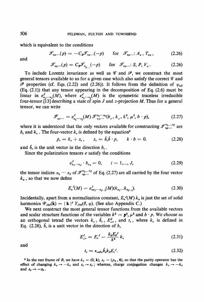
To include Lorentz invariance as well as V and B, we construct the most general tensors available to us for a given case which also satisfy the correct Q and 9’ properties (cf. Eqs. (2.22) and (2.26)). It follows from the definition of vnS (Eq. (2.1)) that any tensor appearing in the decomposition of Eq. (2.6) must be linear in e,“,...,(M), where e,J,...,(M) is the symmetric traceless irreducible four-tensor [13] describing a state of spin J and z-projection M. Thus for a general tensor, we can write
(2.27)
where it is understood that the only vectors available for constructing 9$::‘J are b, and k, . The four-vector k, is defined by the equations
pv = k, -I- xv , s, = a,s*p, k.b=O. (2.28)
and 6, is the unit vector in the direction b, . Since the polarization tensors e satisfy the conditions
eh...., * bmi = 0, i = I,..., J, (2.29)
the tensor indices 01~ **. 01~ of Fti::?’ of Eq. (2.27) are all carried by the four vector k, , so that we now define
EolJW> = da,.. .,,#O(k,,.. .k.+J. (2.30)
Incidentally, apart from a normalization constant, E,$M) k, is just the set of solid harmonics g&k) = ] k IJ Y,,(B, v). (See also Appendix C.)
We next construct the most general tensor functions from the available vectors and scalar structure functions of the variables k2 = p2, p2 and b * p. We choose as an orthogonal tetrad the vectors k,, 6,) Ef, , and r, , where k, is defined in Eq. (2.28), 6, is a unit vector in the direction of b,
E& = EvJ - k2 kiGJ k ,, (2.31)
and tv = l ,dk&/. (2.32)
8 In the rest frame of B, we have k, = (0, k), sy = (p,, , 0), so that the parity operator has the effect of changing k, -+ -k, and s, -+ sy ; whereas, charge conjugation changes k, -+ -k,
and s. -+ -s, .

BETHE-SALPETER EQUATION FOR POSITRONIUM 507
The scalar structure functions will be labeled so as to identify the tensor function (X J”, , Tw > etc.) with which they are associated, the total spin and angular momentum J of the state, the components of the basis tetrad used in constructing the tensor, and the behavior under charge conjugation. For example, l V~J?, p2, b . p) will be the scalar structure function occuring in the singlet state of angular momentum J. It is the component of V, in the direction E,, . The minus (or plus) subscript refers to the oddness (or evenness) with respect to the variable b *p and so labels the behavior under charge conjugation (cf. Eq. (2.26)). Unless otherwise necessary, we will suppress the J label as well as the explicit variable dependence in order to simplify notation.
With these preliminaries over, we are ready to write down our tensors. They depend on three independent sets of structure functions. For the ‘J, system, making use of the properties given in Eqs. (2.15), (2.22), and (2.26) and the fact that
E,J(k) = (- l)J-1 E,J(-k), we can write
S = k * E(lS+), (2.33)
P = 0, (2.34)
v, = &k - E(lV,+) + W - E/k2)(11/k-) + Edl?‘~-), (2.35)
4 = 4?&-), (2.36)
To, = :W,&, - E&XT~~-)
+ (WWko~, - k&J k * WTm+)
+ &%,h - &,&WE,+). (2.37)
The “JJ system has the same tensor structure as that given above but with a different set of structure functions, labeled by 3 instead of 1 as a left superscript and having opposite b *p symmetry properties, i.e., + t) - in the subscripts. Thus for the “JJ system, we will have S = k * E(W), etc.
The 3(J - 1)J - 3(J f 1)J system also has a similar tensor structure, but with S +-+ P, V, t) A, and T,, f-) T,,, in Eqs. (2.33)-(2.37). In addition we must change the superscript labels from 1 to 3 and reverse the b . p symmetry label in the V, and A, structure functions. The complete set of equations for this system is given in Appendix B, Eqs. (B.20)-(B.24).
The above three sets of eight structure functions will lead to three sets of eight coupled equations. An equivalent form of this result has also been recently obtained by using helicity states [14]. The advantage of our present method is its particular application to the fermion-antifermion bound-state problem in quantum electro- dynamics.
508 FELDMAN, FULTON AND TOWNSEND
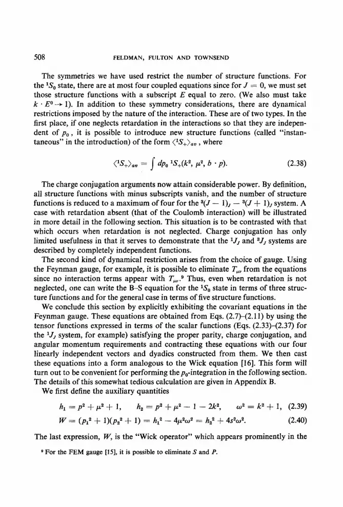
The symmetries we have used restrict the number of structure functions. For the ‘S,, state, there are at most four coupled equations since for J = 0, we must set those structure functions with a subscript E equal to zero. (We also must take k * E” --j 1). In addition to these symmetry considerations, there are dynamical restrictions imposed by the nature of the interaction. These are of two types. In the first place, if one neglects retardation in the interactions so that they are indepen- dent of p. , it is possible to introduce new structure functions (called “instan- taneous” in the introduction) of the form (lS+)av , where
W+>au = 1 &o ‘S+(k2, p2, b . P). (2.38)
The charge conjugation arguments now attain considerable power. By definition, all structure functions with minus subscripts vanish, and the number of structure functions is reduced to a maximum of four for the 3(J - l)J - 3(J + l)J system. A case with retardation absent (that of the Coulomb interaction) will be illustrated in more detail in the following section. This situation is to be contrasted with that which occurs when retardation is not neglected. Charge conjugation has only limited usefulness in that it serves to demonstrate that the lJJ and “JJ systems are described by completely independent functions.
The second kind of dynamical restriction arises from the choice of gauge. Using the Feynman gauge, for example, it is possible to eliminate Tuy from the equations since no interaction terms appear with TuY. s Thus, even when retardation is not neglected, one can write the B-S equation for the ISo state in terms of three struc- ture functions and for the general case in terms of five structure functions.
We conclude this section by explicitly exhibiting the covariant equations in the Feynman gauge. These equations are obtained from Eqs. (2.7)-(2.11) by using the tensor functions expressed in terms of the scalar functions (Eqs. (2.33)-(2.37) for the ‘JJ system, for example) satisfying the proper parity, charge conjugation, and angular momentum requirements and contracting these equations with our four linearly independent vectors and dyadics constructed from them. We then cast these equations into a form analogous to the Wick equation [16]. This form will turn out to be convenient for performing the PO-integration in the following section. The details of this somewhat tedious calculation are given in Appendix B.
We first define the auxiliary quantities
h=P2+p2+1, h, = p2 + ru2 - 1 - 2k2, co2 = k2 + 1, (2.39)
W = (p12 + l)(~,~ + 1) = h12 - 4p2c02 = h22 + 4.~~0~. (2.40)
The last expression, W, is the “Wick operator” which appears prominently in the
e For the FEM gauge [15], it is possible to eliminate S and P.

BETHE-SALPETER EQUATION FOR POSITRONIUM 509
Wick equation [16]. Following the procedure outlined in Appendix B we obtain for the lJJ states the covariant eigenvalue equation
wb(T’+) = lJglYJ+), (2.41)
where d and ‘9. are 8 x 8 matrices and lYJ+ is an 8 x 1 column vector. The superscripts in the wave function indicate a singlet state of angular momentum J and parity (- l)J+l (cf. Eq. (2.15)). The F in l9” refers to the Feynman gauge. The transpose of the wave function is
(VP+) = (lT7&+ ) ‘S+ , IV,+ , IV,- ) IV& , lAt- , lTEk- ) l&t)+).
The 8 x 8 matrix d is given by
c”ii = k * E, i= 1,2,3,4,
bii = E * * El ) bij=O i#j.
I i = 5, 6, 7, 8,
We also define
where
vu = =
and
l$-(lYJ+) = ‘o(lz,)(lYJ+),
10 = (‘3 $,,,
! -2p -h,
h, -2s - 2 2 2k2p 2P 0 -2k2 2s
i h, 2s - 2 2 2~ --hl
-2pk2 -2P 0 ll?, =
In Eq. (2.47) the various interactions are given by
Zl = Zk’ * E’, z4 = hg Z(k,‘E;v - k,‘EL),
I, = k,Zk,’ v , k’ . E’ 15 = -%Jk,’ k’2 ,
(2.42)
(2.43)
ww
(2.45)
(2.46)
(2.47)
(2.48)
Z3 = k,ZE;, , Is = E,*,ZE;, .
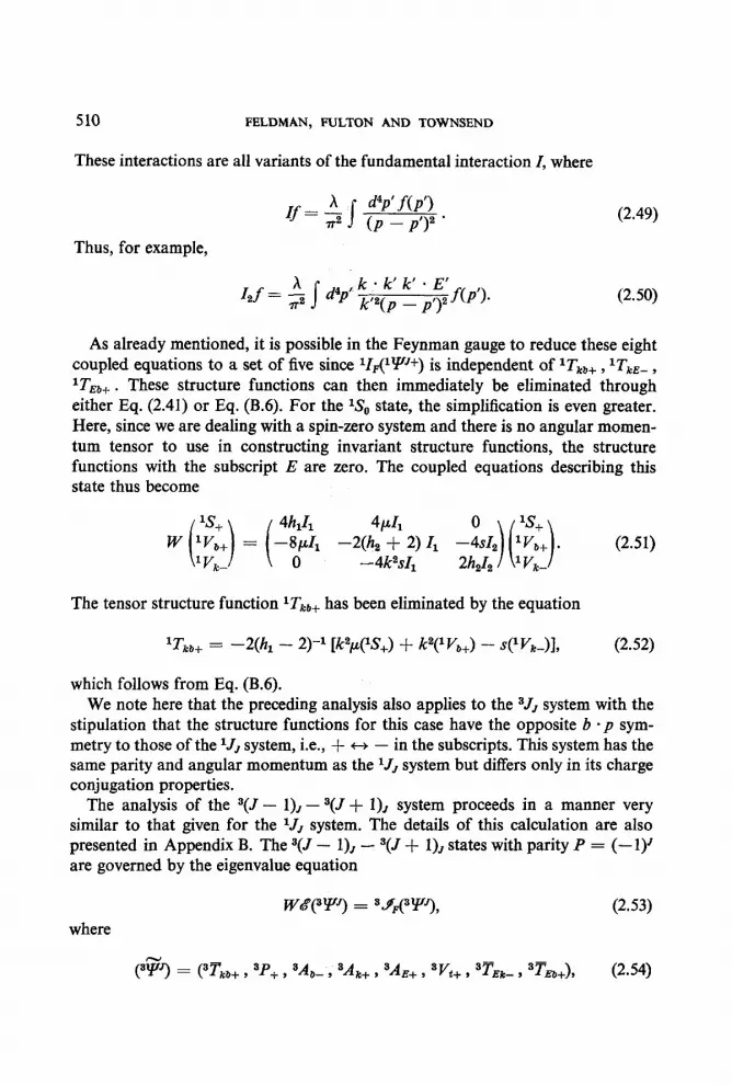
510 FELDMAN, FULTON AND TOWNSEND
These interactions are all variants of the fundamental interaction I, where
If = ; J- d4P’f(P’) . (P - P’)2
Thus, for example,
4f = ; j- d4p’ kt2cp _ ptj2 k * k’ k’ * E’f(p,)e
(2.50)
(2.49)
As already mentioned, it is possible in the Feynman gauge to reduce these eight coupled equations to a set of five since lZp(lYJ+) is independent of IT,,, , lTkE- , lT~a,. These structure functions can then immediately be eliminated through either Eq. (2.41) or Eq. (B.6). For the ‘SO state, the simplification is even greater. Here, since we are dealing with a spin-zero system and there is no angular momen- tum tensor to use in constructing invariant structure functions, the structure functions with the subscript E are zero. The coupled equations describing this state thus become
%I, 4~1, -8cll, -2(h2 + 2) I1 (2.51)
0 -4k2sIl
The tensor structure function lTkb+ has been eliminated by the equation
‘TM,+ = --2(h - W’ [k2pPS+) + k2(‘V,+) - s(~V,+)I, (2.52)
which follows from Eq. (B.6). We note here that the preceding analysis also applies to the “JJ system with the
stipulation that the structure functions for this case have the opposite b -p sym- metry to those of the lJJ system, i.e., + c-) - in the subscripts. This system has the same parity and angular momentum as the ‘JJ system but differs only in its charge conjugation properties.
The analysis of the s(J - l)J - s(J + 1)J system proceeds in a manner very similar to that given for the lJJ system. The details of this calculation are also presented in Appendix B. The 3(J - l), - 3(J + 1X states with parity P = (- 1)’ are governed by the eigenvalue equation
where wciqvJJ) = SJ$(TJ), (2.53)
@‘I = CT&P+ , ‘P,. , 3&- 3 ‘4, , 3A~+, sVt+, sF.k-, 3T~o+>, (2.54)

BETHE-SALPETER EQUATION FOR POSITRONIUM 511
and the matrix d is given by Eq. (2.43). In analogy with the singlet system, we also define
“.q?P) = 30(3Z#PJ), (2.55)
-h, 2k2p 0 2P se, -2~ h, 2 - 2s 2 =
0 -2s h,
i
2s ’
2P -2ka 2sk2 -(hz + 2)
--h, -2,uk2 0 2p h, 2 - se, 2s = 0 -2s h,
2p 2k= -2sk2 and
(2.56)
(3b@)) = (0, 41d3P+), -2z,(3&+), -2&(‘&+) - 2z,(‘&+),
-24d3&+) - 2&(34+), XCVt+), 0, 0). (2.57)
The Z’s appearing in this last equation are given by Eq. (2.48). Just as for the lJJ system, the 3(J - 1)5 - 3(J + l), system of equations can be
reduced to five coupled equations by eliminating 3Tkb+ , 3TEk- , and 3TEb+ using either Eq. (2.53) or Eq. (B25). The simplifications that were present in the lJJ system of equations for the %‘,, state are also present here for the 3P0 state, but we will not present this case explicitly since it is less interesting than the ‘S,, state.
Although by no means trivial, these sets of fully covariant equations are con- siderably simplified from the hitherto familiar expressions. They could serve as a basis for a perturbation approach. That they in fact do so for some simplified interactions is illustrated in the next section.
It is clear from the analysis of Appendix B that one obtains structures similar to that of Eqs. (2.41) and (2.53) in other gauges and even for other than electro- magnetic interactions. The dimensions of Y may become a maximum of four for the IS,, and 3P,, states or eight for the general case, and the detailed structure of Z will vary, but the operators W, d, l@, and 3@ will appear as before.
3. COULOMB INTERACTION
In this section we apply the analysis of Section 2 and Appendix B to the case in which the interaction is instantaneous. For this case, charge conjugation invariance leads to great simplifications. Moreover, we restrict the analysis to positronium

512 FELDMAN, FULTON AND TOWNSEND
for which, of course, the interaction between the bound particles is electromagnetic. We are then able to develop a systematic perturbation theory in terms of effective potentials. In so doing we make contact with previous treatments of this problem.
In order to minimize algebraic complications, we take the instantaneous inter- action to be the Coulomb interaction. For this case Eq. (2.4) becomes
where ti@ + ibr + 1) dP - iY - 1) = Y~~JY~, (3.1)
(3.2)
As in Section 2, we express q in terms of its tensor decomposition Eq. (2.6) and then write the analog of Eqs. (2.7)-(2.11) for the Coulomb interaction. Actually it is not necessary to rewrite all the equations since only the interaction terms are modified. We require the following changes.
Feynman -+ Coulomb
Eq. (2.7): -41s --t -I,S,
Eq. (2.8): 41P + I,P,
Eq. (2.9): 2zv, -+ r, v, - 21, v,s,, ,
Eq. (2.10): -21/I, --+ --I& + 2Z,A,8,, ,
Eq. (2.11): 0 -+a--CT,, + 2T,,&l + 2T,rJu.
(3.3)
The analysis of Appendix B is the same for the Coulomb interaction as long as the replacement lZF , 3ZF -+ lZc , 3Z, is made, where lZc and “Z, are obtained by taking the various projections of Eqs. (2.7)-(2.11) using the right side of Expression (3.3).
The instantaneity of the Coulomb interaction allows us to write
(3.4)
where <d~)>~~ = Jdp,qQ). Thus, if we multiply Eqs. (2.41) and (2.53) by l/W, with the above replacement for the interaction, and integrate both sides of these equations over p. , we reduce them to equations for the p,-integrated (“instanta- neous”) structure functions defined in Eq. (2.38). From the charge conjugation properties, those structure functions with odd b . p symmetry vanish. Therefore, we now delete the remaining + subscripts. Since for the remainder of this section we will be dealing only with PO-integrated structure functions, we will drop the ( )BV symbol from now on for simplicity of notation.

BETHE-SALPETER EQUATION FOR POSITRONIUM 513
We first carry out this procedure for the lJJ system. With the aid of Eqs. (3.3) and (B. 18), we obtain the result
where
cu(w2 - p2) a(?PJ+) = lo(v&lYJ+), (3.5)
(?F+) = (‘Tkb ) 5 IV,, 0, 0, 0, 0, lT,b), (3.6)
(‘Ic e+) = (I2’(lTkb) + &ylTEb), -Ily%s), -I;(lva),
0, 0, 0, 0, +&‘(lTJcb) + 4YTmJ), (3.8) and
11’ = 2 k . E, k*E
1; = ki 5 kd T , Is1 = ki $ ELi ,
Z,’ = ETi $ Eli , k.E
15’ = E:i 2 ki 7 . (3.9)
In writing Eq. (3.5) we have taken the Fourier transform and written the equation directly in coordinate space. With the center of mass at rest, we have k, = (0, k) where k is the differential operator -iv. The symbol w is defined in Eq. (2.39).
From row 8 of Eq. (3.5) we find lTEb = 0. Thus Eq. (3.5) reduces to the simple set of equations
From a comparison of rows 1 and 3 we see that lTkb = k2(lVb). This equality is proved generally for instantaneous singlet wave functions in Appendix C. Elimina- ting lTkb , the two coupled equations can be written
M?4 = 0, (3.11)

514
where
FELDMAN, FULTON AND TOWNSEND
oJ(uJ2 - p2) - co2 fi M=
2r &kfR) ,
4 w(co2 - p2) - ; -
(3.12) R
(3.13)
R=k,%k,-$A. (3.14)
The spin S and orbital angular momentum L are defined in Appendix C. Of course, the L * S term in R does not contribute since the wave functions are scalar densities (not vector).
By taking suitable linear combinations of the rows of Eq. (3.1 l), we can eliminate xv in terms of xs and finally obtain the equation
where uxs = 0, (3.15)
ty=&-- pa- (u+J-)~-~~+J-$~~+&RJ-~ (3.16)
and
xv=-+ ( l-&G xs. )
If we are interested in the binding energy up to order LX~ we may make the approx- imation
k2 oR+1+-,
2 (3.18)
and substitute for p from Eq. (2.3). Also we note that matrix elements of R will be O((Y~). We can then write Eq. (3.15)
to order ma4 as
where
and
(Ho + HI> xs = -Bxs , (3.19)
Ho=k2-f, (3.20)
HI=-R+(+)“-f. (3.21)

BETHE-SALPETER EQUATION FOR POSITRONIUM 515
If we use the identities (k = --iv)
and
k2 $ = 5 k2 + 2ncu. S3(r) + i 5 r . k,
we can write
ki $ ki = 2 k2 + i $ r . k,
ZZ,= -y+ ~ru63(r)+~L.S+$(k2-~+ZS)(k2-
We solve Eq. (3.19) in perturbation theory, i.e., we take
Hoxs 0=-B OXSOY
(3.22)
(3.23)
p + B). (3.24)
(3.25)
so that, to order 01~ in the binding energy, the last term in Eq. (3.24) will vanish when it operates on x So. Accordingly, to order (Ye, the effective Hamiltonian (for the lJJ states) can be written
H eff = k2 - p - y + m iS3(r) + $ L * S. (3.26)
We next discuss the 3J5 system. The equations describing this system are the same as Eq. (2.41), but the structure functions (now labeled with a left superscript 3 instead of 1) have opposite b . p symmetry. Thus, when we consider the Coulomb interaction and integrate over p. , we obtain
c+J2 - p2) S(YJJ) = 1@Z,(W), (3.27)
where @ is given by Eq. (3.7), and d by Eq. (2.43) and
3~J=(o,o,o,v~, 3f'~, 3-4, 3T~~,o); (3.28)
(3Zc-%J) = (0, 0, 0, I,’ “V, + 1; 3V, , Z; 3Vk + 1; 3VE, -Z,’ 3At , -1; 3TEI, , 0) (3.29)
The interactions Z,’ through Z,’ are defined in Eq. (3.9) and
I,’ = $ t, g t, , 1,’ = $ El,,k, g (E,,k, - k,E,,) = I;. (3.30)
By inspection of Eq. (3.27), or using the results of Appendix C, we see that
v, = 0.

516 FELDMAN, FULTON AND TOWNSEND
This gives the coupled equations
3vE
( 1
k2 w(d - p3) EL* - EL 3A, = p
3TEk 1
Again, by inspection of Eq. (3.31) or using Eq. (C.29) we find
3V, = k2(3T,,), (3.32)
and so are led to two coupled equations. Using the results of Appendix C (see Eq. (C.53) we know that the 3JJ wave
function (a vector wave function) must be proportional to t, which in turn is proportional to L (the orbital angular momentum operator). Making use of the fact that the vectors ti , Eli and ki form a mutually orthogonal triad, we can write (using the definitions (2.31) and (2.32))
EL* * El = & ti*ti (3.33)
and
Also, since
we can write t1 cfz Ll , (3.35)
kc 2 kits = - 5 ti a (3.36)
In addition, using Eqs. (C.21) and (3.35) we have the resultlO
L * sti = -t* ) (3.37)
so that, using Eq. (3.14), we further simplify 14’:
14’ = $ tiRti & .
Combining all of these results, we can write the coupled equations for the 3JJ vector wave function ti(3A,) and tiCTEk) as follows:
tiM(3$i> = O, (3.39)
lo The operators S, are to be taken as 3 x 3 matrices whose components are given by (S$l’ = iqR. They are the spin-l operators in the Cartesian representation. The vector wave function X‘ is the ith component of a 3 x 1 column vector in this space. Thus, by using the shorthand notation L + S,yi , we mean Zk L * (S)*$Y~ .

BETHE-SALPETER EQUATION FOR POSITRONIUM 517
where A4 is given by Eq. (3.12) and
Since the operator M cannot connect 3J, states to any others, we can say that the “JJ wave functions can be found by finding the 3J5 solutions to the vector equations
M(3#,) = 0. (3.41)
Now, to find the binding energies to order a*, we proceed as for the lJJ case, with xA( replacing xS and xri replacing xv . The effective Hamiltonian which gives the “JJ binding energies correct to order 01~ is again given by Eq. (3.26).
Lastly, we consider the 3(J f l)J system of equations with the Coulomb inter- action. Integration of Eq. (2.53) over pO with the substitution 31F + 31, results in the equation (We first multiply Eq. (2.53) by l/W.)
where
aJ(02 - p2) 6q3YJ) = q3zc)(?PJ), (3.42)
and
(ep) = (ST,, , SP, 0, 3AI, , 3AE , 3v, ) 0, T&, (3.43)
and
(3Zc(@P)) = (-z;(TkJ - z;(TEJ, Z,‘(SP), 0, -Z,‘(SA,) - Z,‘(SAE),
--1,‘(3A3 - ZL(SAE), Zs’(Vt), 0, -Z5’(T& - z;(T&). (3.45)
By inspection, or using the results (C.27) and (C.28), we have
3A k= -3P, (3.46) and
3TEEb = 3v, . (3.47)
Thus, we have four coupled equations for the four structure functions Fkikb , TEiEb , Ak and AE .

518 FELDMAN, FULTON AND TOWNSEND
We now introduce the 3(J & l)J vector wave functions (See Eq. (C.54)) defined as follows:
kik - E(3Tkb) = k2xTi , (3.48)
Ed’Tm) = p)Ti , (3.49)
kik - E(3A,) E kafAi , (3.50)
E,d3&) = P)Ai . (3.50)
In addition, we have the identities
ki g kjnj = k3 $ kjf, - + L . szt
EG &?i ,
where we have used (C.21), and the fact that
zi a kik . E.
R is first defined in Eq. (3.14). Similarly we have
where
Equations (3.55) and (3.56) are needed in the simplification of I,’ = 1,‘. It follows immediately from Eqs. (3.52) and (3.55) that
and ETtRnt = 0
kiR?d = 0.
(3.52)
(3.54)
(3.55)
(3.56)
(3.57)
(3.58)
Combining all of these results, we can write the four coupled equations as follows:
(k * E) k<M(“$<) = 0 (3.59)
and
E,*,M(%Ji’) = 0, (3.60)
where M is given by Eq. (3.12) and
(3.61)

BETHE-SALPETER EQUATION FOR POSITRONIUM 519
The Eqs. (3.59) and (3.60) are, therefore, not just the ki and Eli projections of a single vector equation. This is a manifestation of the fact that L cannot be used to all orders to label the eigenstates. However, proceeding as in the ‘JJ case, we can write
with
U is given by Eq. (3.16). Further
%J’(xri + wi) = 0, with
(3.62)
(3.63)
(3.64)
E:@A~ + FAi) = -ET*, $ (ma - & (G + R)) (RT~ + q)~i)* (3.66)
Proceeding as for the ‘JJ case, we will find that Eq. (3.62) becomes (to O(OL~))
W-4 + W@T~ + m-i) = -Bk& + n-i), (3.67)
where H, and HI are given by Eqs. (3.20) and (3.21). We find that Eq. (3.64) becomes
-%X-& + H,‘>&t + wi) = --BE~iGri + w-i), (3.68)
where
H,’ = HI + $ k2 - k2 %. (3.69)
When we solve these equations in perturbation theory, we see that, to order a4,
HI’ m HI , (3.70)
since
($0 , f- k2 - k2 :, lb,,) = ($0, (F)” - f 4, - (f)” + 4,:) A) = 0, (3.71)
where I,& is a solution to the Schrodinger-Coulomb equation (3.25). Accordingly, to O((Y~), the 3(J f I), solutions will be the vector wave functions which are eigen-
520 FELDMAN, FULTON AND TOWNSEND
states of Herr (Eq. (3.26)) and which are linear combinations of L = J & 1 func- tions. Since
[L2, Heft] = 0, (3.72)
we can label the eigenstates by L.
4. CONCLUSION
The equations presented in this paper open up two main avenues for further work. First, there is the perturbation calculation of the bound-state energies of positronium. A possible starting point for such a calculation is the retention of the one-photon exchange in the instantaneous radiation gauge and the one photon virtual annihilation as the interaction kernel. This interaction, replacing the Coulomb interaction in the calculations of Section 3, should give the energy levels to order ma4. One must however exercise some care in going to the limit of no retardation for exchanged transverse virtual photons. As we intend to show in a subsequent publication,ll pair terms are suppressed in going to this limit correctly. If one ignores this fact, one obtains incorrect energies, even to order ma4.
The procedures outlined in this paper would then enable us to extend the calcula- tion of both wave functions and energy levels for the instantaneous radiation gauge to higher accuracy. These results could, in turn, be used as bases for a perturbation calculation to solve the more complex B-S equation for positronium, including retardation and multi-photon effects, and could permit the extension of ground state energy calculations to order ma 6. The advantage of the present approach over previous perturbation theories in which calculations are carried out using spinors, is that, despite appearances to the contrary, it is a more straightforward and direct, and more important still, a far more systematic approach. A note of caution must be appended here however. Our present approach in no way obviates the need for “binding corrections,” which can be dealt with systematically in one way by replacing free particle propagators by CoulombGreen’s functions in the kernels of the B-S equation [17]. These replacements will constitute an awkward, though by no means impossible, procedure. A simplification of this approach is desirable before an actual calculation of positronium hfs to order ma6 is attempted.
Another possibility raised by our new approach is that of developing a covariant perturbation theory, based on the equations of Section 2. These equations could
I1 In this paper we also present a detailed comparison of our techniques with previous methods used to solve the Bethe-Salpeter equation in the static limit. See, G. FELDMAN, T. FIJLTON, AND J. TOWNSEND, Correct no-retardation limit in BetheSalpeter kernels, Phys. Rev. A, 8 (1973), 1149.

BETHE-SALPETER EQUATION FOR POSITRONIUM 521
also lead easily to a two variable spectral function representation of the structure functions [18], which again opens up new directions in treating this problem. Still another consequence of the covariant approach is the greater freedom it provides in the choice of gauges and the possibility it offers for the discussion of the gauge independence of the positronium energy levels. Of course, “binding corrections” have to be dealt with in the covariant as well as the non-covariant approach.
Lastly, judging from the work of Kubis [14], it should be possible to extend the methods of the present paper to Helium, in the approximation in which nuclear recoil is neglected. The problem in this case would reduce to the analysis of the motion of two electrons in a static external field. The states would, of course, have to be labeled differently from positronium, and arguments based on the Pauli exclusion principle would replace those based on charge conjugation.
APPENDIX A
The various y matrices are defined as follows:
1 0 Yo=i 0 -17 ( 1 Y = (2a i), y5 = -iy0mw3 = --i (i $ (A.11
% = & [Yn 3 YPL {Yn 9 YJ+ = --2&w 9 {Y5 9 YJ+ = 0. 64.2)
Some useful relations [4], needed for deriving Eqs. (2.7)-(2.11) are
4Y= -a.b+iab cl l/Jo, 3
Cyd = a * by5 + tc,voo4wo,, ,
4yoP = I--a,& + a - bL - dd y,, + ~k,k,,,y,y, ,
4~~~~16 = b&o - a * b&,, + aJ,l y5yo + ia,k,,,,y, ,
4~b, = -GA - aA) + •aB~vaabBy5
+ 1-a . bGL + &&,A + avbh - Lk,b, + &Jl co,, , P + iC - (p - $4 = 2ib,y,,
(P + il) y5 - y5(11- iY) = ---~P,Y~Y, ,
(P + iY) yn - y,(@ - $1 = --2ib, + &P,o,, ,
(P + G9 YF,Y~ - r5rn(l - N = %,Y, - i~,m,pba~op,
(P + N G - 4.P - W = 4ip,yy - 2ik,,,,y5y, .
64.3)
64.4)
(A.3
(A.61
64.7)
(‘4.8)
64.9)
(A.10)
(A.ll)
(A.12)
522 FELDMAN, FULTON AND TOWNSEND
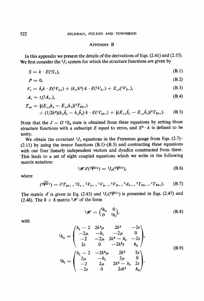
APPENDIX B
In this appendix we present the details of the derivations of Eqs. (2.41) and (2.53). We first consider the lJJ system for which the structure functions are given by
S = k * E(?Y+),
P = 0,
V, = 6Jc * E(‘V,+) + (k&W k * WV,-) + EAVE-),
-4 = G(1-4-),
Tn, = Wd, - E&XTm-1
(B.1)
0-W
03.3)
03.4)
+ (WW(k,& - k&J k - WTm+) + B(E,,& - E,,&)(%,+). (B-5)
Note that the J = 0 ?S, state is obtained from these equations by setting those structure functions with a subscript E equal to zeros, and E” * k is defined to be unity.
We obtain the covariant ‘J, equations in the Feynman gauge from Eqs. {2.7)- (2.11) by using the tensor functions (B.l)-(B.5) and contracting these equations with our four Iinearly independent vectors and dyadics constructed from them. This leads to a set of eight coupled equations which we write in the following matrix notation:
1.x? s(?P+) = fI#P), 03.6) where
(@+) = (lTm+, IS+, IV,+, IV,-, lVE_, l&e, lTm-, IT,,+). (B.7)
The matrix d is given in Eq. (2.43) and lI#I’J+) is presented in Eqs. (2.47) and (2.48). The 8 x 8 matrix l%’ of the form
with
lhz =
lie = (“d- ;,,,
‘h, - 2 2k2p 2k= -2s -2,~ -hl -2p 0 -2 -2p 2k2 - h, -2s
,2s 0 -2k=s h,
‘h, - ‘h, - 2 2 -2k”p -2k”p 2k2 2k2 2s 2s 21-4 21-4 --h, --h, 2cL 2cL 0 0 -2 -2 2p 2p 2k2 - 2k2 - h, h, 2s 2s ’ ’ -2s 0 -2s 0 2sk= h, 2sk= h,
(B-8)
(B-9)

BETH&SALPETER EQUATION FOR POSITRONIUM 523
The auxiliary symbols used in Eq. (B.9) are listed in Eq. (2.39). The following projections have been used to obtain the above result [Xi indicates the ith row of the 8 x 8 matrix Eq. (B.6)]:
R,: 2k,6, projection of Eq. (2.1 I), R,: Eq. (2.7), R3: 6, projection of Eq. (2.9), R,: k, projection of Eq. (2.9), R,: Efp projection of Eq. (2.9), R,: toe/k2 projection of Eq. (2.10), R,: 2ETok,,/k2 projection of Eq. (2.1 l), R,: 2ElfI,6, projection of Eq. (2.11).
In order to obtain Eq. (2.41) it is necessary to invert the matrix l.# so that all the explicit p-depencence is on the right side of the equation. This inversion can be done directly but it is easier to reorder the matrix by adding rows and columns. Reordering rows is accomplished by matrix multiplication from the left, and reordering columns by matrix multiplication from the right. In particular, we choose the following transformations (Ci denotes the ith column):
R1’ = RI - R3, R,’ = R, - R,,C;=C3-Cl,C;=C,-C5. (B.lO)
We let the matrix lM provide the row reordering and lN the column reordering. Thus,
(B.ll)
with
(B.12)
Multiplying Eq. (B.6) by lM, we put it in the form
(1~ 1% ‘jjq’N]-1 b(lYJ+) E lS’[lN]-’ b(?P+) = lM(lr,)(lYJ+), (B.13)
where
(B.14)

524
and
FELDMAN, FULTON AND TOWNSEND
1x, = ( h 2w5.L
-2p -h, 1 ’ 1 7
lY, = (
-4 -2s -20~s 1 h, '
‘Zu = ( -2 zs -2p 1 , ()
(B.15)
In this form the inverse of l.Z’ is easily calculated to be
( ‘X, 0
[lp]-’ = & 0
-l-G lYt4 lx, o
0 --1zg lY, 1
, (B.16)
where W is the Wick operator (cf. Eq. (2.40)). Solving Eq. (B.13), we obtain
q?PJ+) = W[‘iw]-1 (‘M)(lI#PJ+), (B.17)
from which Eq. (2.41) follows since
+I = ‘ivpw]-1 (‘iv). (B.18)
For future reference we note that
I dp, G = ,(,P3 p2) (i ?j j i).
For completeness we now repeat the preceding analysis for the 3(J- I), - 3(J + I), system. The structure functions are given by
s = 0, (B.20)
P = k . Et3P+), (B.21)
V” = t”Cvt+), (B.22)
A, = hk . E(3AtJ + $l k * EC3Ak+) 4 Ed3&+), (B.23)
7, = kpus [ Elakd3Tm-) + +$ k - E(%+) + ~,Jd%d]. 05.24)

BETHE-SALPETER EQUATION FOR POSITRONIUM 525
Contraction of Eqs. (2.7)-(2.11) results in the 8 x 8 matrix equation
33&(V) = 3l#P’), where
(B.25)
(3i?‘) = (3Tk,+ , 3P+, 3Ab-, 3A,+, 3A,+, “V,, , 3T~fi-, 3T~b+). (B.26)
The matrix 8 is the same as for the ‘JJ system and ‘I,(“Y”> is given by Eq. (2.57). The matrix 3X is of the form
3% = p $J (B.27)
with
!
--h, 2k2p 0 -2Y 3h, -2~ h, - 2 -2s -2 =
0 2s hz -2~ 2k2 2k2s -(h, 2: 2kz)
--hl -2k2y 0 -2P h, - 3/z, 2cL 2 -2s 2 =
0 2s h, -2s -2~ -2k2 -2k2s -(h, - 2k”)
I. (B.28)
The following projections have been used to obtain the rows of the above equation:
R,: 2~,~,&& projection of Eq. (2.1 I), R,: Eq. (24, R,: 5, projection of Eq. (2.10), R,: k, projection of Eq. (2.10), R,: ET, projection of Eq. (2.10), R,: t,*/k2 projection of Eq. (2.9), R,: 2q,,,BE~mkB/k2 projection of Eq. (2.1 l), R,: 2~,,,~E~~6~ projection of Eq. (2.11).
To make inversion simpler, we again reorder rows and columns:
i R,’ = -R3, R,’ = R, - R4, R,’ = 3, -t R, ,
c,’ = c, - c, ) c,’ = c, + c, .
This is accomplished by using the matrices
3&f= 3m, 0 ( 0 ) 3rrll ’ 3N = e ;$, (B.29)

526 FELDMAN, FULTON AND TOWNSEND
with
amu= (; ; -; j)? %= (; j ; gy 1
i 0 0 0 0
(B.30)
3ml=3nl= 1 0 o o 1 o .
0 1 0
0 1 1
With this reordering, Eq. (B.25) becomes
where 3iv yAq-1 ciq?P) = 3M(31F)(3Y’),
3.iv = “M(3&@)(3N),
The 2 x 2 matrices “X, , 3Y, , etc., are given by
3x, = ( -h, 2wzp
) 3x1 =
( --h, -2pw=
-2p hl ’ 2~ ) h ’ 3Y, =
( --h, -2s
) 3Yl =
( h, -2s
-2s~~ h, ’ -2s~~ ) -hz ’
“2, = -2 (B 3 3zz = 2 ( 0 -s -P 1 1 *
The inverse of 3&” is then calculated to be
Thus, solving Eq. (B.31), we obtain the result
S(?P) = 3N[32+r’]-1(~M)(3I#P),
(B.31)
(B.32)
(B.34)
(B.35)

BETHI-SALPETER EQUATION FOR POSITRONIUM
from which Eq. (2.53) follows since
$39 = W[3X’]-1 (3&f),
527
(B.36)
with 3O given by Eq. (2.56). The integration over p0 now gives
APPENDIX C
In this Appendix we wish to find the relation between the structure functions of the instantaneous B-S wave function and conventionally defined spin-zero (singlet) and spin-one (triplet) wave functions for a system of two spin-$ particles. These conventionally defined wave functions are, in momentum space x(p) for the singlet case and x,(p)(m = -f 1, or 0) for the triplet case.
The instantaneous B-S wave function in momentum space is
q&k) = s dp, 1 d4x eip.s (0 I ~[$&/2) M--x/w B) b5ha 9 (C-1)
where 01, /3, 6 are spinor indices. Note that k = p. Carrying out the p,, integration in Eq. (C.l) gives
y(k) = (2~) s d3x e-ik*x (0 I W2) !&-x/2) I B> Y5 * (C-2)
By making an expansion of the Schrodinger operators #(x/2) and $(-x/2) into electron-positron annihilation and creation operators we can put certain restric- tions on y(p). We write12
* ($) = &is Zj2 J- d39 h2 + 1)-1’2 x [u(q, s) u(q, s) eiq.Xi2 + b+(q, s)(iy,) u(q, s) e--iqaX/2], (C.3)
I2 The y matrices used throughout this appendix are defined in Appendix A.

528 FELDMAN, FULTON AND TOWNSEND
and the similar expansion for $(x/2). The spinor u(q, s) is the conventionally defined positive frequency spinor and the conventional [I91 u(q, s) is given by the equation
1 iy,u(q, s’)(iu2)*‘* = u(q, s). (C.4) S’
This implies that a+(% 4 0) (C.5)
creates an electron state of spin component s in the rest frame, whereas
b+(s, $1 0) (C.6)
creates a positron of spin component --s in the rest frame. We will see below why we have chosen this convention. Substituting Eq. (C.3) into Eq. (C.2) we obtain
v(k) = c KWw) 4k s> CC--k, SW I 0, s> W--k, $3 I B) 88’
+ (2+) &u(-k,s)P(k,s')iy5 (0 1 b+(-k,s)a+(k,s')I B)] (C.7)
+ two other terms,
where OJ = (k2 + 1)lj2. W.8)
The two terms not written down are of the form
(0 I a@, 4 a+&, 01 B), (C-9)
(0 / b+(-k,s)b(-k,s')l B). (C.10)
Since ) B) is a state of positronium with quantum numbers for P, C and .7 listed in Eqs. (2.15) and (2.17), expressions (C.9) and (C. 10) will vanish.
If we define the projection operators (with unit mass),
and A+(k) = Hl - iy,w - Y * k), (C.11)
.Ukl = &Cl + iyow + Y . k), (C.12)
we see that F(k) must satisfy the relations
U4 v(k) A+(k) = 0, (C.13) and
fl+(-k)cp(k)A-(-k) = 0. (C.14)
In a perturbation expansion, we can expect the second term in (C.7) to contribute only when the vacuum contains pairs. This will not be the case for any instan-

BETHE-SALPETER EQUATION FOR POSITRONIUM 529
taneous potential (such as the Coulomb potential) to lowest order. Thus we should expect the stronger set of equations
n-(k) q+,(k) = 0, (C.15)
vo(k>U--k) = 0 (C.16)
to hold, where q,(k) is the wave function to lowest order. Let us now examine the spin characteristics of the wave functions
and xdk) = (0 I a(k, s) M-k, s’)l B) (C.17)
R&) = (0 1 b+(-k, s) a+@, s’)j B). (C.18)
Because of the choice of spin components specified by (C.5) and (C.6), we may write
xdk) = L,xotk) + (6, xi@), (C.19)
where the ui are the usual Pauli matrices, x0(k) is a singlet wave function, and the xi(k) are triplet wave functions in the Cartesian representation.
If Si are the spin-one operators in wave function space, we have (for example)
&WN~)(Xl(k) + iX2Q) = +lt-u.\/~)txl(b) + ix2tw (C.20)
More generally Six&) = hcxlctk). (C.21)
The vector wave function xi is to be considered as the ith element of a 3 x 1 column vector on which the 3 x 3 matrices Sj act. This notation is explained in footnote 10. If we substitute (C.19) and the similar result for a x,,,(k) into (C,7), we can obtain the y matrix decomposition of the singlet and triplet wave function. For example, for the singlet case we must have
rpor) = s [; W% 3) CC--k, 3) xc,(k) + 1 iyd--k, s) U(k, s) &j&(k)] (C.22) s
= 5 k-4x0 + %I - hdxo - x0) + WUX~ - zJ1. (C.23)
From the definition of the structure functions given by Eqs. (2.33)-(2.37), this implies that only the structure functions l3 ?S, ‘V, and lTkb can contribute to the singlet system and that
k2(lV,) = lTf& . (C.24) (See also Eq. (3.10)).
I3 See Eqs. (2.33)-(2.37) and the discussion following Eq. (3.4) regarding the notation used here.

530 FELDMAN, FULTON AND TOWNSEND
For the triplet case, we will have
(C.25)
+ (-- 28 wm& + &J - 1) &4)(Xi + Ri)
+ B(i) %,rY&(Xr + z31. (C.26)
If we consider the component of xi in the direction of ki and Iook at the definitions of the structure functions, we have
8P = --8Ak. (C.27)
Similarly taking xi in the direction of E,, , we find
and taking xi in the direction ti where t( is defined in Eq. (2.32), leads to
((2.29)
Let us now look at the orbital and spin decompositions of the wave functions xs&). We note that th e b ound states 1 B) are linear combinations of the states ( JM; LS) where J is the total angular momentum, M the z-component, L the magnitude of the orbital angular momentum, and S the magnitude of the spin angular momentum (0 or 1). For the singlet case S = 0, L = J, M = ML, and, therefore,
Xd@> = bXO@~~ (C.30)
where
~004 = Al k I) P’(i) = g(l k I) k . EJ.
(C.31)
Now we consider the triplet case. We will show that any state I JM; Ll) for arbitrary L can be written as some linear superposition
I JM; Ll) = c [LLI 1 JMi> a + ki I JMi) j? + (k x L), I JMi> 71. (C.32) 2

BETHE-SALPETER EQUATION FOR POSITRONIUM 531
The ket 1 JMi) describes a state of orbital angular momentum J and orbital z- component M. It is a state of spin one in the Cartesian representation, i.e.,
L2 1 JMi) = J(J + 1)1 JMi), (C.33)
L, 1 JMi) = M 1 JMi), (C.34)
Si 1 JMj) = iclii / JMl), (C.35)
S2 1 JMi) = 2 1 JMi), (C.36)
and is taken to be orthonormal, i.e.,
(JMi ) JM’j) = &&,~ .
Using the commutation relations for the Li and ki , it follows that
J2 C Oi 1 JMi) G (L2 + 2L * S + S2) C Oi 1 JMi) z z
= C OiL2 I JMi)
= i(J + 1) C Oi 1 JMi),
where Oi is any one of LI , ki or (k x L)i . Similarly
J3 C O+ I JMi) = M C Oi I JMi). t *
Also, one has immediately,
L2 C Li I JMi) = J(J + 1) C Li I JMi). * *
Thus, for the case L = J, we have
(C.37)
(C.38)
(C.39)
(C.40)
For the cases L = J f 1, we must find suitable linear combinations of the states Ci ki I JMi) and Ci (k X L)i I JMi). (Ci Li 1 JMi) is excluded by parity con- siderations).
Using the properties of the operators given above we find
c L * Sk6 I JMi) = - c [2kt I JMi) + i(k x L)i I JMi)], (C.41) I
C L * S(k X L)i I JMi) = C [liiL2 1 JMi) - (k X L), I JMi)]. (C.42) * 2

532 FELDMAN, FULTON AND TOWNSEND
Now, the state I JAI; J + 1, 1) is an eigenstate of L . S with eigenvalue -(J + 2), so that we may write
- (k x L)i I JM) y]
L.SIJM;J+l,l)
= -(J + 2) c [k, I JAB> fi t
= - T [(2/l 1 iyJ(J + 1)) ki I JMi) + ($3 + y)(k x L), 1 JM)], (ca43)
the solutions to which give
I JM; J + 1, 1) = LcJ + l)(iJ + 1j11,2 T KJ+ 1) ffi 1 JMi) + i(h X Lb 1 JMi>l. (C.44)
Similarly we obtain
1 JM; J - l, 1) = [J@J; 1>1’,” T [-J& I JMi) + i(ff x L), I JMi)]. (C.45)
We now make use of Eqs. (CM), (CM), and (C.45) to find the vector form of the triplet wave functions in x&k).
We write
xss*(k) = <0 I a(k, s) b(-k, s') ( JM; 1;l)
= c (0 1 a(k, s) b(-k, s') OF' 1 JMi), e.n
(C.46)
where Ojn) are again one or more of the operators Li , ki and (k x L)( (with the suitable normalization constants,)
We introduce the complete set of states 1 k, j) and obtain
xss@) = C (0 I 0, s> N--k, ~‘1 I k j>@, j I &’ I JM> u.n
= C (~,)""'f(l k I) Si,Op'(L) Y,"(A) c.i.n
(C.47)
where we have used the fact that the coefficients (u$“’ (Pauli matrices) are just the Clebsch-Gordan coefficients in combining two spin-4 particles (recall Eqs. (C.5) and (C.6)) to form spin one in the Cartesian representation. Also we have
<k I LMc> = Yi%, (C.48)

BETHE-SALPETER EQUATION FOR POSITRONIUM 533
and the O,(k) are such that
I&) = i(V, x k), ,
ii(R) = ki ) (C.49)
(i x L)&) = (L x L(& . (C. 50)
Thus the vector wave functions defined in Eq. (C.19) are
xi(k) x J%@ V”‘(~~, for 3J5 (C.51)
xi(k) cc &YJM(l) and (k x L(& YJM(k), for 3(J f l)J. (C.52)
Accordingly, in terms of the orthogonal triad defined in Section 2, we have
xi@) = ti for “JJ, (C.53)
xi(k) cc &k - EJ and E:i for 3(J f 1)5. (C.54)
Parity considerations dictated our choice of identifications above. Identical considerations follow for the wave function f&,(k) defined in Eq. (C. 18).
ACKNOWLEDGMENTS
One of us (T. F.) would like to thank the Aspen Center for Physics for its hospitality during his stay there when part of this work was being done. He would also like to thank Wayne Repko for helpful conversations.
REFERENCES
1. E. E. SALPETER AND H. A. BETHE, Whys. Reu. 84 (1951), 1232; For a complete list of references on the Bethe-Salpeter equation up to 1969, see N. NAKANISHI, Progr. Theoret. Phys. (Kyoto) Suppl. 43 (1969), 1.
2. J. S. GOLDSTEIN, Phys. Rev. 91 (1953), 1516. 3. A. BASTAI, L. BERTOCCHI, S. FUBINI, G. FURLAN, AND M. TONIN, Nuovo Cimento 30 (1963),
1512.
4. W. KUMMER, Nuouo Cimento 31 (1964), 219; Erratum 34 (1964), 1840. 5. N. NAKANISHI, Phys. Rev. 137 (1965), B1352; J. Math. Phys. 12 (1971), 1578. 6. R. KARPLUS AND A. KLEIN, Phys. Rev. 87 (1952), 848. 7. T. FULTON AND P. C. MARTIN, Phys. Rev. 93 (1954), 903; 95 (1954), 811. 8. T. FULTON, D. A. OWEN, AND W. W. REPKO, Phys. Rev. Lett. 24 (1970), 1035; Phys. Rev. A 4
(1971), 1802.
9. E. R. CARLSON, V. W. HUGHES, AND I. LINDCREN, Bull. Amer. Phys. Sot. 17 (1972), 454. 10. R. A. FERREL, thesis, Princeton University, 1951, unpublished.

534 FELDMAN, FULTON AND TOWNSEND
11. W. BARKER AND F. GUIVER, Phys. Rev. 99 (1955), 317. 12. T. FULTON, thesis, Harvard University, 1954, unpublished. 13. C. ZEMACH, Phys. Rev. 140 (1965), B97.
14. J. K~LSIS, Phys. Rev. D 6 (1972), 547. 15. L. EVANS, G. FELDMAN, AND P. T. MATI-HEWS, Ann. Phys. N.Y. 13 (1961), 268. 16. G. C. WICK, Phys. Rev. 96 (1954), 1124; R. E. CIJTKOSKY, Phys. Rev. 96 (1954), 1135.
17. T. FULTON AND R. KARPLUS, Phys. Rev. 93 (1954), 1109, and Refs. [6] and [7]. 18. G. FELDMAN AND T. FULTON, Phys. Rev. D 8 (1973), 3616.
19. J. D. BJORKEN AND S. D. DRELL, “Relativistic Quantum Fields,” McGraw-Hill, New York, 1965.


