Embed Size (px)
Citation preview

Eur. Phys. J. B 37, 55–78 (2004)DOI: 10.1140/epjb/e2004-00030-4 THE EUROPEAN
PHYSICAL JOURNAL B
Glass models on Bethe lattices
O. Rivoire1,a, G. Biroli2, O.C. Martin1, and M. Mezard1
1 LPTMS, Universite Paris-Sud, 91405 Orsay Cedex, France2 Service de Physique Theorique CEA-Saclay, Orme des Merisiers, 91191 Gif-sur-Yvette, France
Received 23 July 2003Published online 19 February 2004 – c© EDP Sciences, Societa Italiana di Fisica, Springer-Verlag 2004
Abstract. We consider “lattice glass models” in which each site can be occupied by at most one particle,and any particle may have at most occupied nearest neighbors. Using the cavity method for locally tree-like lattices, we derive the phase diagram, with a particular focus on the vitreous phase and the highestpacking limit. We also study the energy landscape via the configurational entropy, and discuss differentequilibrium glassy phases. Finally, we show that a kinetic freezing, depending on the particular dynamicalrules chosen for the model, can prevent the equilibrium glass transitions.
PACS. 64.70.Pf Glass transitions – 64.60.Cn Order-disorder and statistical mechanics of model systems –75.10.Nr Spin-glass and other random models
1 Introduction
The thermodynamics of vitreous materials is a long stand-ing yet very alive subject of study [25]. In spite of muchresearch, it remains unclear whether this “amorphous”state of matter can exist in equilibrium; even if it can-not, probably the underlying crystalline equilibrium phaseis irrelevant for understanding the physics of glassy sys-tems. As experience has shown in other contexts, a lot ofunderstanding can be gained by looking at models sim-ple enough to be analyzed but that retain the essentialphysics. Following this strategy, several recent works havefocused on lattice models for structural glasses.
Lattice gas models with hard core exclusion, i.e., witheach site being occupied by at most one particle, de-signed to reproduce the glass phenomenology, fall into twodistinct classes. A first class consists of kinetically con-strained models [23] which have a glassy behavior forcedby a dynamical constraint on allowed moves, but oth-erwise trivial equilibrium properties. An example is theKob-Andersen model [12] where a particle is allowed tomove only if before and after its move it has no morethan some number m neighboring particles. In this casethe slow dynamic displays several remarkable propertieslike for example an avoided transition toward a coopera-tive “super-Arrhenius” dynamics [27]. Physically, the ki-netically constrained models are based on the assumptionthat the glassy behavior is due to an increasing dynamicalcorrelation length whereas static correlations play no role.Thus, the possibility of a thermodynamic glass transitionis excluded from the beginning.
a e-mail: [email protected]
In contrast, the models we will discuss here belongto a second class where the glassy features are generatedthrough a geometric constraint on allowed configurations.In this case a thermodynamic equilibrium glass transi-tion independent of the chosen local dynamical rules mayexist. Indeed, as we shall show in the following, it takesplace for models on a Bethe lattice. Such models werefirst introduced in reference [3] and some variants havebeen elaborated since then [5,29].
In this paper, we study the lattice glass models on“Bethe lattices” which are random graphs with a fixedconnectivity. This kind of approach provides an approxi-mation scheme for the lattice glasses on Euclidean latticeshaving the same value of the connectivity, in the sameway as the Bethe approximation allows one to computeapproximate phase diagrams of non frustrated systems.Furthermore this approximation can be improved system-atically, at least in principle, by implementing higher ordercluster variational methods. But this random graph studyis also interesting for its own sake. In particular we ana-lyze in detail the limit of diverging chemical potential. Inthis limit, one recovers an optimization problem which isthe lattice version of close-packing of spheres, a problemthat has challenged mathematicians for many decades [7]and is still matter of debate today [26].
With respect to their Euclidean counterparts, the lat-tice glasses on Bethe lattices have one important differ-ence: the existence of the random lattice, even with fixedconnectivity, forbids crystalline ordering. This loss is alsoan advantage in that the absence of crystal phases makes iteasier to study the glass phase. Indeed, when the density ofthe system is increased, we find a thermodynamical phasetransition from a liquid phase to a glass phase. We can

56 The European Physical Journal B
determine the phase diagram analytically, focusing in par-ticular on the liquid to glass transition. In many systemsthis transition is of the “random first order” [8–11] type,also called “one-step replica symmetry breaking” [17]. Onthe Bethe lattice there are actually two transitions: whenincreasing the density or chemical potential, one first findsa dynamical transition in which ergodicity is broken, thena static phase transition. The intermediate phase is suchthat the thermodynamic properties are those of the liq-uid phase, in spite of the ergodicity breakdown. At thestatic transition the entropy and energy are continuous,with a jump in specific heat. Therefore the Bethe-latticeglass models provide clear solvable examples of a systemof interacting particles exhibiting the scenario for the glasstransition which was proposed in [8–11] by analogy withsome spin glass systems. This scenario is known to be amean-field one, which does not take into account the nu-cleation processes that can occur in Euclidean space. It isgenerally believed that nucleation processes transform thedynamical transition into some cross-over of the dynam-ics from a fast one to a slow, activated relaxation [4,8–11].Whether the static transition survives in realistic systemis unknown so far. In this paper we will not discuss the rel-evance and modifications of the mean field scenario whenapplied to finite dimensional problems since we have noth-ing to add to existing speculations. Let us just mentionthat the lattice glasses provide the best examples on whichthese issues can be addressed. The first step of such astudy is to have a detailed understanding of the meanfield theory, and this is what we do in the present paper.
Note that some of the results have appeared in ref-erence [3]; here we give a new and extensive discussionon the nature of the different possible equilibrium glassyphases.
On top of the thermodynamic study, we have also stud-ied the dynamical arrest of the lattice glasses on Bethelattices. The dynamical arrest depends on the specific dy-namical rule that is implemented. We show that this dy-namical arrest is in general unrelated to the energy land-scape transitions found in the thermodynamic approach.In particular, in some models, a dynamical arrest takesplace at a density smaller than the one of the dynami-cal glass transition. In kinetically constrained problems,such mean field arrest transitions are known to becomecrossovers in finite dimensional systems. The correspond-ing arrest behavior on our lattice glass models is notknown yet.
The outline of this paper is as follows. In Section 2, weintroduce the models on lattices of arbitrary types and de-fine the relevant thermodynamics quantities. In Section 3,we address the case of loop-less regular lattices, calledCayley trees when surface sites are included and Bethelattices when surface effects can be neglected. We showthat low densities correspond to a liquid phase describedby the Bethe-Peierls approximation, but that inhomoge-neous phases must be present at higher densities. However,the strong boundary dependence of models on Cayley treesdoes not allow one to define such dense phase in the in-terior. To overcome this problem, we consider instead in
Section 4 random regular graphs; they share with Cayleytrees a local tree-like structure but are free of surface ef-fects and thus provide a natural generalization of Bethelattices adequate for dense phases. Our study on randomgraphs is performed by means of the cavity method [18]which predicts for high densities a glassy phase. In Sec-tion 5, we focus on the close-packing limit and discuss indetail the nature of this glassy phase. Finally in Section 6,we comment on the differences between the equilibriumglass transition of our models and the kinetic transitions ordynamical arrests related to specific local dynamical rules.In particular we show that for some models the dynamicalarrest takes place before the equilibrium glass transition.
2 Lattice models
2.1 Constraints on local arrangements
When packing spheres in three dimensions, the preferredlocal ordering is icosahedral; this does not lead to a peri-odic crystalline structure and is the source of frustration.To model this type of frustration, we forbid certain localarrangements of the particles on the lattice. This can bedone using two or n-body interactions. We follow [3] andset the interaction energy to be infinite if a particle hasstrictly more than particles as nearest neighbors. Theinteractions thus act as “geometric” constraints.
Note that these geometric constraints are very similarto the kinetic constraints of the Kob-Andersen model [12].However, as we shall show, the fact that they are encodedin an energy function makes a big difference physically, inparticular for the thermodynamic behavior.
We work in the grand canonical ensemble and intro-duce a chemical potential. All energies being zero or infin-ity, temperature plays no role. The thermodynamics for agiven system (i.e., a given lattice) is then defined by thegrand canonical partition function
Ξ(µ) =∑
n1,...,nN∈0,1C(n1, . . . , nN ) eµ
∑Ni=1 ni . (1)
The dynamical variables are the site occupation values:ni = 0 if site i is empty and ni = 1 if a particle is on thatsite. We take all the particles to be identical. In equa-tion (1), µ is the chemical potential, and C(n1, . . . , nN)implements all the geometrical constraints: it is the prod-uct of local constraints, one for each of the N sites. Theterm for site i is
θ
− ni
∑j∈N (i)
nj
(2)
where N (i) denotes the set of neighbors of i, and θ(x) = 0if x < 0, θ(x) = 1 if x ≥ 0.
For sake of concreteness and simplicity, we will focus inthe core of the paper on the = 1 case when each particlehas at most one neighbor, deferring the general case toAppendix A. Most numerical results will be given for the“basic model”, noted BM, for which = 1 and k = 2.
O. Rivoire et al.: Glass models on Bethe lattices 57
2.2 Observables
For a given “lattice” of N sites and type (Euclidean, tree,random graph, . . . ), and for a given form of constraints(i.e., a value of ), there is only one parameter, the chem-ical potential µ. It is useful to introduce the grand poten-tial µΩ(µ) and its density ω(µ) ≡ Ω(µ)/N , so that
Ξ(µ) = exp [−µΩ(µ)] = exp [−Nµω(µ)] . (3)
The pressure is given by p = −µω(µ) and the particledensity is
ρ(µ) ≡⟨∑
i ni
N
⟩=
1NΞ(µ)
dΞ(µ)dµ
= −d(µω)dµ
=dp(µ)dµ
.
(4)Clearly, ρ is an increasing function of µ. When µ→ −∞,the system becomes empty, a typical equilibrium configu-ration having almost all ni = 0, so ρ→ 0. In the oppositelimit, µ→ +∞, there is in effect a strong penalty for eachvacancy, but the geometrical constraints prevent all sitesfrom being occupied; then ρ has a maximum value strictlyless than 1. When N →∞, this value is expected to con-verge to a limit ρ∞. Obviously, ρ∞ depends on the typeof lattice and on the parameter .
We can define similarly the entropy density s(µ):
s(µ) ≡ lnΞ(µ)N
− µρ(µ) = −µω(µ)− µρ(µ) (5)
where again s(µ) should have a well defined thermody-namic limit.
Other physical quantities that we shall study includesusceptibilities associated with two-site connected correla-tion functions of the type 〈ninj〉c. At low densities the ni
have only short range correlations. When µ increases, ρalso increases; then the constraints become more impor-tant and correlations grow. When the density is closeto ρ∞, the system will be very “rigid”, allowing few fluctu-ations in the local density. It is plausible that the suscep-tibility will diverge at some critical value of µ, separatinga liquid phase at low µ from a denser phase at large µ.
The nature of this dense phase, and of the transition,will depend on the lattice, on the boundary conditions,and need not be associated with a crystalline order. Whenit is not crystalline, we want a statistical description ofthe dominant equilibrium configurations. In particular, ifthese configurations form clusters, it is of interest to es-timate the number of such clusters. We will do this bycomputing the “configurational entropy”Σ(ρ) (also calledcomplexity) associated with the number of clusters (alsocalled states) of configurations with a given density ρ.
3 Models on Cayley trees
3.1 Iteration equations
We first consider glass models defined on regular trees, i.e.connected graphs with no loops and fixed connectivity.
i
j=1 j=k
Fig. 1. An iterative method is used to compute the partitionfunction on rooted trees. We begin with k rooted trees withroots j = 1, . . . , k and form a new rooted tree by joining a site ito each of them. The possible occupations of site i depend onthe occupations of the sites j = 1, . . . , k and on the type ofconstraint used.
We distinguish rooted trees where a site called the rootis connected to only k neighbors while all the other sites(except for those at the surface, that is the leaves of thetree) have k + 1 neighbors. A Cayley tree is obtained byconnecting a site to the roots of k + 1 rooted trees.
When the graph is a rooted tree, the grand canonicalpartition function can be computed by recursion startingfrom the leaves. To do this, we follow conditional parti-tion functions because we need to know how to apply theconstraints when joining the sub-trees (cf. Fig. 1). Thisprovides a generalization of the well-known transfer ma-trix method for one dimensional systems (which can beviewed as rooted trees with k = 1).
In our class of constraints, we need to know whetherthe root sites are occupied, and if they are, whether theyhave occupied neighbors or less than that. Let Ξ(e)
i ,Ξ
(u)i and Ξ
(s)i be the conditional partition functions for
a rooted sub-tree i when its root node i is empty (e),occupied but the constraint unsaturated (u) and finallyoccupied and the constraint saturated (s), i.e., the rootsite has neighboring particles. Then the conditional par-tition functions for the rooted tree obtained by joining thesub-trees are easily computed.
For instance, in the = 1 case where each particle canhave at most one neighbor, when merging k rooted trees(j = 1, . . . k) to obtain a new tree rooted say at site i, wehave
Ξ(e)i =
k∏j=1
(Ξ
(e)j +Ξ
(u)j +Ξ
(s)j
), (6)
Ξ(u)i = eµ
k∏j=1
Ξ(e)j , (7)
Ξ(s)i = eµ
k∑j=1
Ξ(u)j
∏p=j
Ξ(e)p . (8)

58 The European Physical Journal B
Naturally, the total partition function is the sum of theconditional partition functions.
To study these recursions, it is convenient to considerlocal fields defined via ratios of conditional partition func-tions. Here we introduce on a root site i two fields ai and bidefined as
e−µai ≡ Ξ(e)i
Ξ(e)i +Ξ
(u)i +Ξ
(s)i
, (9)
e−µbi ≡ Ξ(e)i
Ξ(e)i +Ξ
(u)i
. (10)
The first quantity is the probability for the root of a rootedtree to have an empty site (e); the second is the ratio ofthat probability and the probability to have a non satu-rated site. The use of µ when defining these fields is tosimplify the analysis at large µ (cf. Sect. 5). These twofields form a closed recursion under the joining of sub-trees; for instance when = 1,
ai = a(a1, b1, . . . , ak, bk)
=1µ
ln
1 + eµ(1−∑k
j=1 aj)
1 +
k∑j=1
(eµbj − 1
) ,(11)
bi = b(a1, b1, . . . , ak, bk)
=1µ
ln[1 + eµ(1−∑k
j=1 aj)]. (12)
Note that the use of ratios of conditional partition func-tions leads to recursions for two quantities rather than theinitial three. To recover all the information in the initialrecursions, we also keep track of the change in the grandpotential. If Ω1, . . .Ωk give the grand potentials of the ksub-trees, we have after the merging
Ωi =k∑
j=1
Ωj +∆Ωiter(a1, b1, . . . , ak, bk) (13)
where ∆Ωiter(a1, b1, . . . , ak, bk) = ∆Ωiter is defined via
e−µ∆Ωiter =Ξi∏k
j=1 Ξj
=Ξ
(e)i +Ξ
(u)i +Ξ
(s)i∏k
j=1
(Ξ
(e)j +Ξ
(u)j +Ξ
(s)j
) .(14)
With our definition of the fields, we have then ∆Ωiter =−a. From here on, we shall use the short-hand notation:h ≡ (a, b) and hi = h(h1, . . . , hk) with
h (h1 = (a1, b1), . . . , hk = (ak, bk)) =(a(a1, b1, . . . , ak, bk), b(a1, b1, . . . , ak, bk)
). (15)
3.2 Liquid phase
Begin now on the leaves of a rooted tree, assuming thatsome kind of boundary condition is specified there. For
example, the ni could be fixed, or their probability distri-bution could be given. These determine the initial valuesof the conditional partition functions and thus of the fields.We iterate the recursions, propagating the fields awayfrom the leaves by performing mergings. When µ −1,these iterations are contracting and so the fields convergeto a value that is independent of the starting values on theleaves. The distribution of fields in the bulk (away fromthe leaves) is then given by
P(h) = δ(h− hliq) (16)
with the fixed point condition hliq = h(hliq, . . . , hliq). Wedetermine the fixed point for all µ, and refer to it as theliquid solution; its physical relevance includes at least theregion µ −1.
We can now merge consistently k + 1 rooted trees toobtain a Cayley tree. We then have a liquid (or param-agnetic) phase, all correlations being short range and theheart of the Cayley tree being insensitive to the boundaryconditions, even though a finite fraction of the sites liveon the surface. In this regime, the homogeneous interiorof the Cayley tree can be used to define the Bethe latticemodel.
In this context, also known as the Bethe-Peierls ap-proximation, the density ω can be obtained from the fol-lowing construction. Start with (k + 1) Bethe lattices;for each of them, pick an edge and remove it, leading to2(k + 1) infinite rooted trees. Then form two Bethe lat-tices by adding two sites and connecting each to (k + 1)of the rooted trees. Now the difference in grand potentialbetween the resulting two Bethe lattices and the initialones is just twice the grand potential per site (since twosites were added) and can be written as
2ω = −(k + 1)∆Ωedge + 2∆Ωsite (17)
where ∆Ωedge is the difference in grand potential corre-sponding to adding an edge and ∆Ωsite to merging (k+1)branches into a new site. Such quantities are easily ex-pressed with the partition functions of rooted trees; forinstance for = 1 we obtain
e−µ∆Ωsite(a1,b1,...,ak+1,bk+1) =
1 + eµ(1−∑k+1j=1 aj)
1 +
k+1∑j=1
(eµbj − 1
) (18)
and similarly
e−µ∆Ωedge(a1,b1,a2,b2) =[Ξ
(e)1 Ξ
(e)2 +Ξ
(e)1
(Ξ
(u)2 +Ξ
(s)2
)+
(Ξ
(u)1 +Ξ
(s)1
)Ξ
(e)2
+Ξ(u)1 Ξ
(u)2
]/(Ξ1Ξ2)
=e−µ(a1+a2)(eµa1 + eµa2 + eµ(b1+b2) − eµb1 − eµb2
).
(19)

O. Rivoire et al.: Glass models on Bethe lattices 59
-0.2
-0.1
0
0.1
0.2
0.3
0.4
0.5
0.6
-6 -4 -2 0 2 4 6 8 10 12µ
ρ
s
µ =
µm
od
Fig. 2. µ dependence of the particle density ρ and entropy sof the liquid phase for the BM ( = 1, k = 2). The failure ofthe liquid phase to correctly describe the model at high µ isevidenced by the negative sign of the entropy for µ > µs=0 7.40. But in fact the liquid solution becomes linearly unstablewell before, at µmod 2.77 (vertical line).
Note that we have the simple relation
∆Ωsite(h1, . . . , hk+1) = ∆Ωiter(h1, . . . , hk)
+∆Ωedge
(h(h1, . . . , hk), hk+1
)(20)
whose interpretation is clear: the addition of one site bymerging k+1 rooted trees T1, . . . , Tk+1 can be decomposedinto the construction of a new rooted tree T0 obtained bymerging a site to the k rooted trees T1, . . . , Tk and theaddition of an edge between T0 and Tk+1. Moreover∆Ωsite
is obtained from ∆Ωiter by making the substitution k →k+ 1. The expressions (18–19) are written for the generalinhomogeneous case but simplify in the liquid phase whereall the fields take their liquid value.
In Figure 2, we show as illustration the liquid’s den-sity ρ and its entropy density s, as a function of µ forthe BM. Since the models are discrete, the equilibriumentropy should never go negative. Nevertheless, the liquidsolution at large µ, µ > µs=0, leads to sliq < 0 except invery special cases such as k = 1. Thus there must exist aphase transition at µc ≤ µs=0, and the liquid phase can-not be the equilibrium phase at µ > µc. Clearly, one mustdetermine when the liquid solution is physically relevant;when it is not, one should find other solutions [3].
3.3 Linear stability limit of the liquid
The Bethe-Peierls approximation fails when the bulkproperties of the Cayley tree become sensitive to theboundary conditions. This “instability” may show up viaa loss of stability of the fixed point equations as given bya simple linear analysis. Indeed, starting with fields iden-tically and independently distributed on the leaves, the
field distribution Pg+1(h) at “generation” g + 1 is relatedto that at generation g by
Pg+1(hi) =∫ k∏
j=1
dhjPg(hj)δ(hi − h(h1, . . . , hk)
).
(21)Close to a liquid solution we have to first order
〈δh〉g+1 = k∂h
∂h1
∣∣∣∣liq
〈δh〉g (22)
where δh ≡ h − hliq and 〈.〉g refers to the average usingthe distribution Pg. Since h is a two-component vector,∂h/∂h1 is actually a 2× 2 Jacobian matrix. If λ1 denotesthe eigenvalue of largest modulus of that matrix, the sta-bility criterion simply reads
k|λ1| ≤ 1. (23)
When k|λ1| > 1, the liquid solution is unstable to pertur-bations homogeneous within a generation; we shall refer toit as the modulation instability because it is a transition toa regime with successive (homogeneous) generations car-rying different fields.
An alternative point of view consists in studying re-sponse functions. At finite µ, the response to a pertur-bation is related to correlations through the fluctuation-dissipation theorem, and an instability can be detected bymeans of a diverging susceptibility. Thus, we recover theprevious result by computing the linear susceptibility inthe liquid phase, looking for the point where it becomesinfinite. The linear susceptibility is defined in terms ofconnected correlation functions 〈ninj〉c via
χ1(µ) ≡ dρ
dµ=
1N
∑i,j
〈ninj〉c. (24)
Making use of the homogeneity of the liquid solution, itcan be rewritten
χ1(µ) = ρ(1− ρ) +∞∑
r=1
(k + 1)kr−1〈n0nr〉c (25)
where n0 and nr are taken at distance r in the tree. Theseries converges provided that
ln k + limr→∞
ln〈n0nr〉cr
< 0. (26)
To evaluate 〈n0nr〉c, we invoke the fluctuation-dissipationrelation
〈n0nr〉c =∂〈nr〉∂h
(c)0
(27)
where h(c)0 denotes the external field conjugate to n0. Since
h(c)0 is a function of (the components of) h0 only, we can
use the chain rule
∂〈nr〉∂h
(c)0
=∂〈nr〉∂hr−1
(r−1∏l=1
∂hl
∂hl−1
)∂h0
∂h(c)0
(28)

60 The European Physical Journal B
where we introduced hl ≡ h(hl−1, hliq . . . , hliq) as inter-mediate fields. In the liquid phase, all these fields areequal and the previous equation factorizes, leading againto k|λ1| ≤ 1. For instance for the BM, the modulationinstability shows up at µmod = 4 ln 2 2.77, well beforethe entropy becomes negative at µs=0 7.40 as shown inFigure 2.
3.4 Crystal phase
We can ask whether it is possible to choose boundary con-ditions such that the interior of the Cayley tree has a peri-odic structure (for a general tree, the boundary conditionswill vary from leaf to leaf). In the µ→∞ limit, we expecta crystalline phase to exist whose structure can be eas-ily displayed by starting at the center of the Cayley tree,filling the sites with particles whenever possible. In thiscase, for the BM, the field h = (a, b) takes three differentvalues he, hu and hs such that
he = h(hs, hs),
hu = h(he, he),
hs = h(he, hu), (29)
with he = (0, 0), hu = (1, 1) and hs = (1, 0). The in-teger values 0 and 1 of the components of these fieldsreflect the fact that a given site is certainly empty, unsat-urated or saturated. For finite µ, fluctuations are presentbut we can still look for a fixed point of equation (29),with he, hu, hs ∈ R.
Such a solution, distinct from the liquid one, is foundto exist and to be stable for µ ≥ µms with µms 2.89 (msfor melting spinodal). Next we want to evaluate the grandpotential of this crystalline solution in the bulk. To do so,we first consider the µ =∞ limit and estimate the densityof empty and occupied sites, ρ0 = 2/5 and ρ1 = 3/5, andalso the proportion of edges connected to one and twoparticles, π1 = 4/5 and π2 = 1/5. Then the crystallinepotential can be written as ωcryst = ωsite−3/2 ωedge, with
ωsite = ρ0∆Ωsite(hs, hs, hs) + ρ1∆Ωsite(hu, he, he),
ωedge = π1∆Ωedge(he, hs) + π2∆Ωedge(hu, hu). (30)
Now for µms < µ <∞, the structure of the crystal is pre-served, with empty and occupied sites being replaced bymost probably empty or occupied site. Therefore we resortto equation (30), using the adequate values of the fieldshe, hu, hu, and we keep the same factors ρ0,1 and π0,1.This leads to a melting transition (where ωliq = ωcryst) atµm 3.24.
Comparing µms 2.89 with the location of the liquid’sinstability µmod 2.77, we have an interval µmod < µ <µms where no homogeneous nor periodic solution seemsto exist. This is to be contrasted with the phase diagramof the hard sphere model studied by Runnels [24] wherethe presence of a particle on a site forbids the occupation
of any of its neighboring sites. That model has been re-considered recently in two dimensions as a combinatorialproblem of counting binary matrices with no two adjacent1’s when µ = 0 [2] and on random graphs as an optimiza-tion problem called vertex cover problem when µ =∞ [28];from the point of view of our lattice glasses, these modelscorrespond to the = 0 constraint. In this case the modu-lation instability coincides exactly with the melting tran-sition (and with the spinodal point), µm = µms = µmod.This is due to the special structure of the crystal, or-ganized in alternate shells of empty and occupied sites,and therefore described by a cyclic solution of the liquidequation, h1 = h(h0, . . . , h0) and h0 = h(h1, . . . , h1) withhomogeneous shells (i.e., the arguments of h are all iden-tical). For = 1 no such cyclic solution was found andhomogeneous boundary conditions on the leaves yield anaperiodic behavior of the recursion hj+1 = h(hj , . . . , hj).This feature is very specific to the unphysical nature ofpure Cayley trees: it does not survive in the random reg-ular graphs which we use below. Therefore we have notpushed its study any further.
4 Models on random regular graphs
4.1 From Cayley trees to random regular graphs
When the Bethe-Peierls approximation no longer holds ona Cayley tree, the sensitivity to boundary conditions doesnot allow one to define a thermodynamic limit and there-fore may lead to unphysical results. Since that is due tothe presence of a finite fraction of the sites on the surface,one way to get rid of this problem is to define Bethe lat-tice models as models on random regular graphs. These aresimple graphs with fixed connectivity k+ 1, simple mean-ing that they have no trivial loops (joining a site to itself)and no multi-edges (no two edges join the same sites).Here we will use the cavity method to obtain results for atypical random graph (chosen uniformly in the set of allrandom regular graphs with a fixed connectivity k + 1).
When the number N of sites is large, typical randomregular graphs look locally like trees, having only longloops of order lnN . Therefore the recursive equations still(locally) hold, making these lattices analytically tractable.The large loops implement an analog of generic boundaryconditions and the resulting frustration forbids crystallineorderings. One then expects the system to possess an equi-librium glass phase in the high µ region.
In the low µ phase, the liquid solution is recovered. Thecorresponding Bethe-Peierls approximation is called thefactorized replica symmetric approximation in the contextof the cavity method where the vocabulary is inheritedfrom the treatment of spin glasses based on the replicatrick. However the glassy high µ regime will be character-ized by the existence of many solutions of the local equa-tions and we will have to resort to the replica symmetrybreaking (rsb) formalism to correctly take into accountthe specific organization of these solutions [15].

O. Rivoire et al.: Glass models on Bethe lattices 61
4.2 Entropy crisis
Reconsidering the stability of the liquid with the modu-lation instability now being excluded, we can look for a“spin-glass” instability, to borrow the terminology frommagnetic systems where the modulation instability is re-ferred to as the “ferromagnetic instability”. This new in-stability manifests itself as a divergence of the non-linearsusceptibility, which is defined as
χ2(µ) ≡ 1N
∑i,j
〈ninj〉2c . (31)
In the formalism of Section 3.3, the instability appears asa widening of the variance 〈(δh)2〉g under the recursion ofequation (21). Both approaches are equivalent and lead toa stability criterion
k|λ1|2 ≤ 1. (32)
The eigenvalue λ1 is the same as for the linear suscepti-bility since the transfer matrix is just the square of theJacobian matrix we had in equation (22). Note that thiscondition is always weaker than that for the modulationinstability, k|λ1| ≤ 1. However it is the relevant one inthe case of random graphs where homogeneous perturba-tions are generically incompatible with frustration. If theliquid is locally stable for all µ, a continuous phase tran-sition is excluded. For = 1 this happens for k = 2, 3because
√k|λ1(µ)| < 1 for all µ with only asymptotically√
k|λ1(µ)| → 1 as µ→∞. In the general case, as soon asµg > µs=0, where µg (g for glass) is defined by
√k|λ1(µ = µg)| = 1, (33)
the resolution of the entropy crisis requires a phase tran-sition before the spin-glass local instability is reached,and we conclude that a discontinuous phase transitionmust take place at µc ≤ µs=0. In that case we expecta behavior similar to that of infinite-connectivity mod-els solved within a one-step replica symmetry breaking(1-rsb) Ansatz, like e.g. the p-spin models (p > 2). Whenµg < µs=0, as is found for = 1 and k ≥ 4, we can ei-ther have a continuous transition at µg or a discontinuoustransition at µc < µg; a study of the local stability of theliquid solution says nothing about which case arises.
4.3 Cavity equations
The solution by the cavity method predicts results forquantities averaged over all random regular graphs withsize N →∞, but the problem is more clearly stated on agiven finite regular graph. Indeed, we want to solve self-consistently a set of (k + 1)N coupled equations for thecavity fields
hi→j0 = h(hj1→i, . . . , hjk→i)∀i ∀j0, j1, . . . , jk ∈ N (i) (34)
whereN (i) denotes the set of k+1 neighbors of i. Thus foreach i ∈ 1, . . . , N we have k+1 equations correspondingto the different choices of j0 ∈ N (i). The notation hi→j
refers to the local field on i when the edge to the site j isremoved, and it is called a cavity field; for a Cayley tree,it corresponds to the field on the root i of a rooted treeobtained when the edge ij has been removed. These localequations are known as the TAP equations in statisticalphysics [17] and as the belief propagation equations incomputer science [13]. The contact between both pointsof view has recently lead to establish that these equationsmust always have at least one fixed point corresponding tothe minimum of a correctly defined Bethe-Peierls approx-imated free energy [30]. Their solutions should correspondto the fuzzy concept of states ubiquitous in the spin-glassliterature.
A message passing algorithm can be used to try tosolve these equations on a given graph of large but fi-nite size N . First on each oriented edge we associate localfields hi→j randomly initialized. Then we proceed itera-tively: at each step, all the oriented edges are successivelychosen in a random order, and the field on the chosen ori-ented edge is updated by taking into account the valuesof its neighbors as prescribed by equation (34). The iter-ation is stopped when a sweep of all the oriented edgesresults in no change; in such a case we lie at a fixed pointof the local equations. However the algorithm may alsonot converge, in which case no conclusion can be drawn.In practice, we find a rapid convergence toward the liquidsolution for µ < µbp and then a failure to converge forµ > µbp. The critical µbp depends slightly on the graphbut for large N and large k, it is given by the glass in-stability, i.e., µbp → µg as k → ∞. In some case (for nottoo big graphs), we could find a convergence towards anon-liquid distribution, suggesting that the high µ regioncorresponds in fact to a glassy phase. In order to dealwith this phase where the Bethe-Peierls approximationbreaks down and simple message passing algorithms fail,we will now introduce the cavity method which providesboth an alternative approximation for infinite graphs andinsights into elaborating more efficient algorithms for fi-nite graphs [18]. In Appendix D we present an alternativeapproach based on the replica method.
4.4 One-step replica symmetry breaking cavity method
The local equations equation (34) can be written for arbi-trary graphs but they provide exact marginal probabilitydistribution (and thus exact particle densities) only fortrees. In addition, they are in general intractable. How-ever, they are particularly suited for very large randomgraphs, where due to the local tree-like structure, they areexpected to provide good approximations of the marginalsand where additional hypotheses allow for an analyticaltreatment. To do so, we do not try to find one solu-tion but instead turn to a statistical treatment of sets ofsolutions.
Being interested in the case where many solutions ex-ist, we fix a µ for which this is supposed to happen.

62 The European Physical Journal B
We make the further hypothesis that exponentially many(in N) solutions exist. More precisely, we assume that thenumber NN (ω) of solutions with a given potential den-sity ω on graphs of size N is given by
NN (ω) ∼ exp[NΣ(ω)] (35)
where Σ(ω) ≥ 0 is called the configurational entropy (orcomplexity) and is supposed to be an increasing and con-cave function of the grand potential ω. This is a stronghypothesis which is justified by its self-consistency and byits consequences (in particular it matches with the outputof replica theory calculations, cf. Appendix D).
Starting with a graph G, we pick a site i and oneof its neighbors j0 ∈ N (i), and define the graph Gi→j0
as the connected graph containing i obtained by remov-ing the edge ij0 from G. If G is a Cayley tree, Gi→j0 isnothing but a rooted tree, the appropriate structure towrite down recursive relations. We introduce Ri→j0 (h, ω),the joint probability density, when a solution α of equa-tion (34) defined on Gi→j0 is chosen randomly, that thecavity fields h(α)
i→j0on i take the value h and the grand
potential density ω(α)i→j0
the value ω,
Ri→j0 (h, ω) =1Nsol
∑α
δ(h− h(α)
i→j0
)δ(ω − ω(α)
i→j0
).
(36)The next crucial hypothesis is based on the locally
tree-like structure of large random graphs. Indeed, ifthe graph Gi→j0 is a rooted tree, the sub-rooted treesGj1→i, . . . ,Gjk→i with j1, . . . , jk ∈ N (i) are disjoint andthe cavity fields hj1→i, . . . , hjk→i are therefore solutionsof uncoupled local equations. In such a case the jointprobability distribution factorizes over the independentvariables
R(hj1→i, ωj1→i; . . . ;hjk→i, ωjk→i) =
Rj1→i (hj1→i, ωj1→i) . . . Rjk→i, (hjk→i, ωjk→i) . (37)
In addition, a simple relation between the distributionRi→j0 on a rooted tree Gi→j0 and the Rj1→i,. . . ,Rjk→i onits sub-rooted trees Gji→i,. . . ,Gjk→i can be written:
Ri→j0 (h, ω) =∫ k∏
r=1
dhjrdωjrRjr→i (hjr , ωjr)
× δ(h− h (hjr)
)
× δ[ω − 1
N
(k∑
r=1
Njrωjr +∆Ωiter(hjr))]
(38)
where the Njr are the sizes of the sub-trees and N =∑r Njr + 1 is the size of Gi→j0 . A further simplification
takes place on regular trees where, due to the absenceof local quenched disorder, the equations for hj1→i,. . . ,
hjk→i are identical. In such a case, Ri→j0 is in fact inde-pendent of the oriented edge i → j0. For a large randomregular graph, we assume that the same properties hold.Note that the last hypothesis, yielding Ri→j0 = R is calledthe factorization approximation and could be relaxed byworking with a distribution R[R] of the R over the var-ious edges [15]. However the factorization approximationshould be exact on random regular graph for systems with-out disorder provided that no spontaneous breaking of“translational” invariance occurs, and we will not considerthis extension here.
We now want to write the 1-rsb cavity equation, whichis a self-consistent equation for the distribution P (ω) of lo-cal fields h at a fixed grand potential ω. P (ω) is obviouslyproportional to R, P (ω)(h) ∝ R(h, ω), and since the distri-bution of the ω is given by
∫dhR(h, ω) = C exp[NΣ(ω)],
we have the relation
R(h, ω) = CeNΣ(ω)P (ω)(h) (39)
with C a proportionality constant independent of both hand ω. Next we fix a grand potential density ω0 and con-sider only potentials ω close to ω0, noted ω ∈ Vω0 , suchthat we can linearize the complexity
Σ(ω) Σ(ω0) +mµ(ω − ω0) (40)
withm(ω0) ≡
1µ
dΣ
dω(ω0). (41)
Given the concavity of the complexity Σ, fixing ω0 isequivalent to fixing m and thus Vω0 can be rewrittenas Vm. Plugging relation (39) into equation (38), we findthat the distribution defined by
P (m)(h) ∝∫
ω∈Vm
dωP (ω)(h) (42)
satisfies a simple self-consistent equation
P (m)(h) ∝
∫ k∏j=1
dhjP(m)(hj)δ
(h− h(hj)
)e−mµ∆Ωiter(hj).
(43)
Equation (43) is called the factorized 1-rsb cavity equation.We will drop the explicit reference to the parameter m inthe ensuing discussion, but it should be kept in mind thatthe 1-rsb cavity field distribution P (h) is m-dependent.
As we have seen, it is convenient to fix m insteadof ω; going from ω to m actually amount to performinga Legendre transformation. The complexity Σ(ω) is re-covered by Legendre transforming the function Φ(m) de-fined as
mΦ(m) = mω − 1µΣ(ω) (44)
via the relation
1µΣ(ω) = m2∂mΦ(m). (45)

O. Rivoire et al.: Glass models on Bethe lattices 63
Equation (44) is similar to the definition of the entropythrough
µω(µ) = −µρ− s(µ) (46)
[cf. Eq. (5)]. Indeed Φ(m) is for the states the analog ofthe grand potential ω(µ) for the configurations, the pa-rameter m sampling the states as the chemical potentialµ samples configurations, and the complexity Σ(ω) count-ing states as the entropy s(µ) counts configurations [19].The quantity corresponding to the grand partition func-tion is
Ξ(m) =∑
α
exp[−Nmµω(α)(µ)
]
=∫dω exp (N [Σ(ω)−mµω])
= exp[−NmµΦ(m)]. (47)
Following the same analogy, Φ(m) can be computed simi-larly to a grand potential. To do so, we first need to gen-eralize to random regular graphs the construction that ledus to the Bethe-Peierls approximation of the grand poten-tial, equation (17). Likewise, we want to write
Φ(m) = ∆Φsite(m)− k + 12
∆Φedge(m) (48)
with ∆Φsite(m) the contribution from a site addition, and∆Φedge(m) from an edge addition. The way two sites canbe added is even simpler than for Bethe lattices here be-cause we do not care about introducing loops: take a ran-dom regular graph of size N and connectivity k + 1, pick(k+1) edges and remove them, leading to 2(k+1) ampu-tated sites with k neighbors instead of (k + 1). Then addtwo new sites and connect each one to (k+1) of the ampu-tated sites, leading to a new random regular graph of sizeN+2 and same connectivity (k+1). Thus the contributionto Φ when going from N to N + 2 sites is equivalent tothe contribution from two site additions plus (k+ 1) edgedeletions [i.e., minus (k+ 1) edge additions], as expressedby equation (48).
To see how this is related to the grand potential shifts∆Ωsite and ∆Ωedge, we rewrite equation (39) introducingthe definition equation (41) of the parameter m as
R(h, ω) = emµN(ω−ω(0))P (h) (49)
where ω(0) = ω(0)(m) enforces the normalization. Thefunction
ρ0(Ω) ≡ emµ(Ω−Ω(0)) (50)
gives the distribution of grand potential Ω = Nω ona rooted graph of size N with one site having only kneighbors. Now we take k + 1 such rooted graphs anddetermine the distribution ρ1(Ω) when one site is added.
It is given by
ρ1(Ω) =∫ k+1∏
j=1
dhjdΩjR(hj, Ωj)
×δ
Ω − k+1∑
j=1
Ωj −∆Ωsite(hj)
= emµ
(Ω−∑k+1
j=1 Ω(0)j
)
×∫ k+1∏
j=1
dhjP (hj)e−mµ∆Ωsite(hj)
≡ emµ(Ω−Ω(1)) (51)
with Ω(1) =∑k+1
j=1 Ω(0)j + ∆Φsite, while the mean shift
∆Φsite due to a site addition is
∆Φsite(m)=− 1mµ
ln
∫ k+1∏
j=1
dhjP (hj)e−mµ∆Ωsite(hj)
.
(52)We compute similarly the contribution from edgeaddition,
ρ2(Ω) =∫ 2∏
j=1
dhjdΩjR(hj , Ωj)
×δ
Ω − 2∑
j=1
Ωj −∆Ωedge(h1, h2)
= emµ
(Ω−Ω
(0)1 −Ω
(0)2
)
×∫ 2∏
j=1
dhjP (hj)e−mµ∆Ωedge(h1,h2)
≡ emµ(Ω−Ω(2)) (53)
with Ω(2) = Ω(0)1 + Ω
(0)2 + ∆Φedge, while the mean shift
∆Φedge due to an edge addition is
∆Φedge(m) =
− 1mµ
ln
∫ 2∏
j=1
dhjP (hj)e−mµ∆Ωedge(h1,h2)
. (54)
The replica symmetric description of the liquid phaseis recovered by taking P (h) = δ(h − hliq). When manysolutions coexist, by varying m = m(ω0) at fixed µ, wedescribe states characterized by different values of ω0 andthe question is which m must be selected to describethe equilibrium (glassy) thermodynamics. Following equa-tion (47), the grand partition function is
Ξ(µ) =∫dω exp (N [Σ(ω)− µω]) (55)
and the saddle point method for N → ∞ indicates thatthe grand potential ω of the dominating states is such

64 The European Physical Journal B
that µ = ∂ωΣ(ω). But of course, this saddle equationis relevant only if its solution ωs lies inside the intervalrange ]ωmin, ωmax[ where the integral is performed, whichcorresponds to the range where Σ(ω) is strictly positive.Generically, for µ > µs, it is found that ωs < ωmin, andwe must then take instead ωs = ωmin. A kind of replicatrick intervenes here to balance the complexity contribu-tion thanks to the parameter m, in such a way that ωs
is always given by a saddle equation. So, in the glassyphase µ > µs where the rsb formalism becomes necessary,we want the equilibrium grand potential to be given byωs = ωmin(µ) ≡ Φ(ms). Since the complexity curve is ex-pected to be continuous at ωmin, we can alternatively askfor the condition Σ(ωs) = 0. From equation (45), we seethat it corresponds to extremizing Φ(m), i.e.,
∂mΦ(m = ms) ≡ 0 (56)
which is precisely the criterion provided by the replicamethod for selecting the breaking point parameter m.
Note that other values of m also carry physical infor-mation. Lower values of m (m < ms) describe metastablestates for which ω > ωs (it is the analog of a non-zero tem-perature giving access to excited configurations); of partic-ular interest is the value ωd associated to the maximumcomplexity Σ(ωd) ≡ maxω Σ(ω) since its describes themost numerous states. We expect that this is the portionof phase space where the system will get almost trappedat long times after a “quench” from the low density liquidphase.
Higher values of m (m > ms) are usually termed asunphysical, but in fact they describe properties of systemsassociated with untypical graphs. In particular, it can beshown that m = 1 always gives back the liquid solution.In fact, for m > ms, the cavity method leads to a nega-tive complexity, which seems to be in contradiction withits initial definition equation (41). The point is that in thecavity method, the graph is not specified and eNΣ(ω) is thenumber of states with grand potential ω after averagingover different graph realizations. This fact has no conse-quence whenever the average corresponds to the typicalcase, which is expected as soon as Σ(ω) > 0 ; indeed somegraph realizations may behave very differently from typ-ical realizations, but their contribution to the averagedquantities is negligible. However, an exception is worthmentioning: if the quantity we average is typically strictlyzero, but happen to be positive for exponentially rare real-izations, it leads to a small but non zero (i.e. non typical)average. We find such a behavior here, where some untypi-cal graphs allow for ωs lower than the typical value ω(typ)
s ,leading to a Σ
(ω < ω
(typ)s
)< 0 even if the complexity on
a given graph is intrinsically a positive quantity.An analog phenomenon happens for instance in the
random energy model, where averaging over disorder leadsto a negative entropy associated with energies lower thanthe typical ground state, while for a given realization ofthe disorder the entropy is necessarily positive. Here therole of the quenched disorder is taken by the topologicaldisorder from the various realizations of random regular
graphs. From this point of view, a random graph with nofrustrating loop is an example of untypical graph whichhas a crystalline ground state, as opposed to the glassyground states of typical random regular graphs.
4.5 Observables
To complete our overview of the cavity method, we nowshow on the example of the particle density how physicalobservables can be computed; Section 4.9 will provide another example with the computation of susceptibilities.We begin by considering rooted trees where the particledensity on the root i is simply given by
〈ni〉rooted tree =Ξ
(s)i +Ξ
(u)i
Ξ(s)i +Ξ
(u)i + Ξ
(e)i
= 1− e−µai . (57)
Now for a Cayley tree, we need to take into account k+ 1neighbors instead of k,
〈ni〉Cayley tree = 1− e−µAi . (58)
where the total local field A is computed similarly to thecavity field a but substituting k by k + 1, i.e.,
Ai = A(a1, b1, . . . , ak+1, bk+1)
=1µ
ln
1 + eµ(1−∑k+1
j=1 aj)
1 +
k+1∑j=1
(eµbj − 1)
. (59)
The total field Bi would be defined similarly; note thatwith our notations, we simply have A = −∆Ωsite. On arandom graph in the 1-rsb phase, we need to include thereweighting associated with the addition of the site i:
ρ(µ,m) =
∫ ∏k+1j=1 dhjP (hj)(1− e−µA(hj))e−mµ∆Ωsite(hj)∫ ∏k+1
j=1 dhjP (hj)e−mµ∆Ωsite(hj)(60)
and the equilibrium value is given by ρ(µ,ms). The samelines can be followed to compute any other observables.
4.6 Order parameters
Comparing with the replica method [17], the cavity ap-proach focuses on local fields instead of overlaps betweenstates. In lattice glass models, the latter can be defined as
qαβγ... ≡1N
N∑i=1
〈ni〉α〈ni〉β〈ni〉γ . . . (61)
with the indices α, β, γ, . . . denoting states randomly cho-sen according to their Boltzmann weights.
Overlaps are particularly useful in infinite connectiv-ity systems where, due to the central limit theorem, the

O. Rivoire et al.: Glass models on Bethe lattices 65
first two moments qα and qαβ are sufficient to encode theGaussian distribution of the cavity fields. In contrast, forfinite connectivity systems, an infinite number of overlapsmust be kept and working directly with the local fielddistribution is simpler. However, the two choices of orderparameters, local cavity fields or global overlaps, providecomplete and equivalent descriptions; in particular over-laps can be easily recovered from the knowledge of thecavity field distribution.
At the replica symmetric level, all indices α, β,γ, . . . are equivalent, so we only need to distinguish over-laps according to the number r of states they involve, andwe have
q(rs)r ≡ 〈ni〉r =∫dAdBPrs(A,B)
(1− e−µA
)r(62)
with A and B being the total local fields of Section 4.5.Note that the replica symmetric approximation in princi-ple already involves a functional order parameter Prs, butin our case where the factorization Ansatz is taken, theliquid distribution is trivial and we merely have q(rs)r =(1− e−µAliq)r , i.e. the order parameter is a single scalar.
At the one-step level, we need to distinguish whetherrandomly chosen states are distinct or identical. Thus foroverlaps involving two replicas, we can define two param-eters, q0 ≡ qαβ (α = β) and q1 ≡ qαα, corresponding re-spectively in spin glasses to the Edwards-Anderson orderparameter and the (squared) magnetization. Their com-putation amounts to calculating densities inside a state,which was the subject of the previous section. Note how-ever that q0 and q1 provide only a partial description of thesystem and the full order parameter has here a functionalstructure P (h). Any new level of replica symmetry break-ing will require considering a more sophisticated order pa-rameter, namely a distribution over the order parametersfrom the previous level. For instance, the two-step orderparameter will be written as a distribution Q[P ] over dis-tributions P (h). Describing with this formalism a finiteconnectivity system with full replica symmetry breakingis therefore rather complicated, and we will limit ourselfto at most two levels of replica symmetry breaking in theensuing discussion.
4.7 Solution via population dynamics
Given the cavity equations (43), we would like to solvethem. Since they are essentially functional relations, ananalytical treatment is not possible in general. An impor-tant exception however is the close-packed limit µ → ∞;the next section is devoted to this case. Here we con-sider the more general finite µ situation and use thepopulation dynamics algorithm of reference [15] to ob-tain numerical results. The principle of the algorithm iselementary: the distribution P (h) is encoded in a familyof M fields hii=1,...,M such that
P (h) 1M
M∑i=1
δ(h− hi), (63)
and the cavity field distribution is expressed as the fixedpoint of the iteration equation
Pg+1(h) ∝∫ k∏
j=1
dhjPg(hj)δ(h− h(h1, . . . , hk)
)×e−mµ∆Ωiter(h1,...,hk). (64)
At each step, M new children are generated; each isobtained by choosing randomly k parents among thepopulation. To take into account the reweighting, weduplicate or eliminate the children according to theirweight e−mµ∆Ωiter so that we keep a total population of(approximately) M individuals.
However, such a recursion turns out to be unstableand we stabilize it by means of a relaxation parameter ε ∈]0, 1[. At each step, only a fraction εM of the population isregenerated. The reason for this relaxation will be madeclearer when we will discuss the stability of the cavitymethod solution; it will be associated to the instability ofthe first kind discussed in Section 5.2.2.
4.8 Static and dynamical transitions
At low µ, the population dynamics algorithm always con-verges to the liquid solution, i.e., starting from a pop-ulation with an arbitrary distribution it converges to apopulation of identical fields corresponding to the fixedpoint hliq of h. When µ is increased, a first non-trivialdistribution is found at µ = µd for m = 1. At this pointmany states exist, but they are only metastable and thestatics is still given by the (paramagnetic) liquid state.This ergodicity breaking is called a dynamical phase tran-sition because it is where the equilibrium dynamics shoulddisplay an ergodic-non ergodic transition (see however thediscussion in Sect. 6).
A static phase transition, which is the one relevant atequilibrium, only appears for higher chemical potential,µ = µs, when the configurational entropy vanishes. At thispoint the grand potential of the 1-rsb solution becomeslower than the one of the liquid and the equilibrium phasetransition takes place.
In practice, the dynamical transition point µd is foundby decreasing µ and looking for the µ where the 1-rsb so-lution disappears. For the BM, it happens at µd 6.4;more generally for = 1 and other k we find µd < µs,indicating that the transition is always discontinuous, ascould not be directly inferred from the arguments of Sec-tion 4.2. To obtain µs, we calculate explicitly ∂mφ(m,µ)and look for the µ at which ∂mφ(m = 1, µ) = 0; for theBM, we obtain µs 7.
4.9 Stability of the one-step solution
To determine whether the equilibrium state is really de-scribed by a 1-rsb solution or whether further replicabreakings are necessary, one has to study the stability of

66 The European Physical Journal B
q0
q1
2nd kind
1st kind
x0 1m
q(x)
Fig. 3. Pictorial view of the two possible instabilities of the1-rsb Ansatz. At the bottom, the states stay states but clus-terize (first kind). At the top, the states become cluster of newstates (second kind). If we were on a totally connected graphwhere an overlap function q(x) can be defined, its 1-rsb shapewould be affected on different parts depending on which insta-bility is relevant; indeed its left part (x < m) corresponds tothe inter-state overlap q0 and its right part (x > m) to theintra-state overlap q1.
the 1-rsb solution. In this section we set up the formal-ism needed to check it. In the following sections we willanalyze the stability in the close packing limit (µ→∞).
In the 1-rsb phase the Gibbs measure is decomposedin a cluster of different thermodynamic pure states [17].Thus, there are two different types of instabilities that canshow up [17]. First kind: The states can aggregate intodifferent clusters (see Fig. 3). To study this instability onehas to compute inter-state susceptibilities:
χinterp =
1N
∑i,j
(〈ni〉〈nj〉 − 〈ni〉 〈nj〉
)p
. (65)
where the overline denotes an average over the states takenwith their Boltzmann weights. Second kind: Each statecan fragment in different states (see Fig. 3). To study thisinstability one has to compute intra-state susceptibilities:
χintrap =
1N
∑i,j
〈ninj〉pc . (66)
If any of the intra or inter-state susceptibilities divergethen the 1-rsb glass phase is unstable (toward a 2-rsb glassphase). However, as for the liquid, the linear susceptibil-ities χ1 are related to instabilities incompatible with theunderlying random graph structure and, hence, they are
irrelevant for our purposes. In the following we will focuson the p = 2 case which is the only relevant one sinceall the susceptibilities with p > 2 are clearly bounded inmodulus by the p = 2 one.
Because of the homogeneity of the simple randomgraphs that we are focusing on, the stability analysis issimplified and in particular:
χinter2 =
∞∑r=1
(k + 1)kr−1(〈n0〉〈nr〉 − ρ2
)2
,
χintra2 =
∞∑r=1
(k + 1)kr−1〈n0nr〉2c (67)
where n0 and nr are at distance r (we omitted the unim-portant r = 0 term).
We expect, as it can be proved (see below), that thecorrelation functions decay exponentially at large distance
〈n0nr〉2c ∼ exp(−r/ξ2), (68)
and (〈n0〉〈nr〉 − ρ2
)2
∼ exp(−r/ζ2). (69)
Due to the tree-like structure of the lattice, the result-ing stability conditions are different from the conditionξ <∞ used for finite dimension lattices and reads
ξ2 <1
ln k, ζ2 <
1ln k
. (70)
In the following we show how the correlation length ξpcan be computed. A very similar procedure can be carriedout for ζ2. In Appendix B we shall show explicitly howthis can be done in the close-packing limit (µ =∞).
In order to obtain ξp we need to compute the corre-lation functions 〈n0nr〉pc . We write the generalization ofequation (28) as
〈n0nr〉α,c =(∂〈nr〉∂hr−1
)t(
r−1∏l=1
∂1h(hl−1; gl,j)
)∂h0
∂h(c)0
(71)
where the fields are (d − 1)-dimensional vectors (d = 3for our models), so that the product involves in fact(d− 1)× (d− 1) dimensional Jacobian matrices ∂1h (thenotation ∂1h indicates that the derivative is taken withrespect to the first field, here hl−1, and ()t means trans-posed). Note that h(hl−1; gl,j) is used as a short-handnotation for h(hl−1, gl,1, . . . , gl,k−1) (see Fig. 4). Next weneed to take into account the reweighting introduced bythe addition of the sites l = 1, . . . , r − 1. With a transfer-matrix approach in mind, we write it as
e−mµ∆Ω =Ξ
Ξ(0)(∏r−1
l=1 Υ(l)
)Ξ(r)
=r−1∏l=1
(Ξ(l)
Ξ(l−1)Υ (l)
)Ξ
Ξ(r−1)Ξ(r)(72)

O. Rivoire et al.: Glass models on Bethe lattices 67
r1 r-10
g
1 r-1hh
g1,1 r-1,1
g1,k-1
gr-1,k-1
grh 0
Fig. 4. Cavity diagram for computing a two-site correla-tion function 〈n0nr〉c. As all we know is P (h), the distri-bution of the local field on the root of a rooted tree, webuild a chain of sites l = 0, . . . , r out of rooted trees withfields h0, g1,j , . . . , gr−1,j , gr. We proceed recursively: we firstadd site l = 1, obtain a new rooted tree with root 1 and localfield h1 = h(h0, g1,1, . . . , g1,k−1) so the length of the chain tocompute is reduced from r + 1 to r. Then we proceed furtherby adding site 2, etc (see also Fig. 5).
(0) Υ(1) Υ(2)Ξ (r)Υ Ξ
Υ Ξ(r)ΥΞ(1) (2)
(r-1)
(r-1)
0
2’
1’ 2’
r-1’
r
r
r-1’
0
1
1’
Fig. 5. Partition functions involved in the reweighting forthe computation at the 1-rsb level of the two-site correlation〈nonr〉pα,c, illustrated here with k = 2. We start with the parti-tion functions Ξ(0), Υ (1), . . . , Υ (r−1), Ξ(r) where Υ (l) is in gen-eral the product of the partition functions of k−1 rooted trees(top of the figure); for k = 2 as illustrated, it reduce to onerooted tree with root site noted l′. Next we merge the k rootedtrees corresponding to Ξ(0) and Υ (1) into a site 1 and call thepartition function of the resulting rooted tree Ξ(1) (bottom).Recursively, we define similarly the other Ξ(l) for 2 ≤ l ≤ r−1.
where the notation refers to Figure 5: Υ (l) denotes theproduct of the k − 1 partition functions associated withthe rooted trees with cavity fields gl,j (1 ≤ j ≤ k− 1) andΞ(l) (1 ≤ l ≤ k − 1) the partition function of the rootedtree obtained by connecting a new site l to the k rootedtrees corresponding to Υ (l) and Ξ(l−1).
We can write for one site addition
Ξ(l)
Ξ(l−1)Υ (l)= exp[−mµ∆Ωiter(hl−1; gl,j)], (73)
and for the last edge addition
Ξ
Ξ(r−1)Ξ(r)= exp[−mµ∆Ωedge(hr−1, gr)]. (74)
The 1-rsb formula for 〈n0nr〉pc is therefore
Z−1
∫dh0P (h0)
r−1∏
l=1
k−1∏
jl=1
dgl,jlP (gl,jl
)
dgrP (gr)
×[(
∂〈nr〉∂hr−1
)t(
r−1∏l=1
∂1h(hl−1; gl,j)
)∂h0
∂h(c)0
]p
×(
r−1∏l=1
e−mµ∆Ωiter(hl−1;gl,j)
)e−mµ∆Ωedge(hr−1,gr) (75)
where the normalization Z is given by
Z =∫dh0P (h0)
r−1∏
l=1
k−1∏
jl=1
dgl,jlP (gl,jl
)
dgrP (gr)
×(
r−1∏l=1
e−mµ∆Ωiter(hl−1;gl,j)
)e−mµ∆Ωedge(hr−1,gr). (76)
To be complete, we also need to insert in the previousformulae the following identity defining the intermediatefields hl,
1 =∫ r−1∏
l=1
dhlδ(hl − h(hl−1; gl,j)
). (77)
To determine the behavior of the correlation functionsbetween sites at distance r, we introduce two transfer ma-trices, corresponding respectively to the numerator anddenominator of equation (75),
Tn(hl−1, hl) =∫ k−1∏
jl=1
dgl,jlP (gl,jl
)∂1h(hl−1, gl,jl)
× δ(hl − h(hl−1; gl,jl
))e−mµ∆Ωiter(hl−1;gl,jl
),
Td(hl−1, hl) =∫ k−1∏
jl=1
dgl,jlP (gl,jl
)e−mµ∆Ωiter(hl−1;gl,jl)
× δ(hl − h(hl−1; gl,jl
)). (78)
Finally, calling respectively λ(p)n , λd the largest eigen-
values of the matrices (Tn)p and Td we obtain that forlarge r
〈n0nr〉pc ∼ exp(−r/ξp) (79)

68 The European Physical Journal B
withξp = − 1
ln(|λ(p)n /λd|)
. (80)
Notice that all this discussion of stability of the 1-rsbsolution is not just academic. Indeed simulations per-formed on the BM with the distribution P of the fields gl,j
generated by population dynamics show that, at a fixedchemical potential µ > µd, the correlation length ξ2(m)increases when m is decreased from m = 1 to 0. In ad-dition, the critical length 1/ ln 2 is reached at some finitevalue of m, mc < ms, indicating that the description ofmetastable states corresponding to m < mc requires tobreak the replica symmetry beyond one step.
The limits of the 1-rsb approach will be discussed inmuch more details in the following section devoted to theµ = ∞ limit where it is shown that the [((d − 1)∞) ×((d−1)∞)] transfer “matrices” (the∞ stands for the con-tinuum range of the fields hl so the matrices are actuallyoperators) reduce to finite [(d − 1)d × (d − 1)d] matriceswhose eigenvalues can be computed without resorting tothe population dynamics.
5 Close-packing limit
The zero temperature limit of the cavity method, whichcorresponds in lattice glasses to the µ = ∞ limit, has re-ceived particular attention [16], both because of the sim-plifications it allows and because of its applications to op-timization problems. For lattice glasses, the correspondingoptimization problem, called the close-packing problem,consists in finding, for given lattice and packing constraint,the largest achievable particle density. We will obtain thesolution of this problem as a result of our study.
5.1 One-step rsb Ansatz
We first consider the close-packing problem as a limitingcase of the previous considerations; thus for µ → ∞, thesingle rs equations (11) and (12) simplify to
a0 = max
0, 1−
k∑j=1
aj + max1≤j≤k
bj
, (81)
b0 = max
0, 1−
k∑j=1
aj
. (82)
The advantage of this limit is that we can resort to theexact Ansatz
P (a, b) = peδ(a)δ(b) + puδ(a− 1)δ(b− 1)+(1− pe − pu)δ(a− 1)δ(b). (83)
Note that the simple form obtained here results fromour appropriate choice of the local fields. Other choicesmay lead to a similar Ansatz but with more than threespikes. This minimal number of three is related to the
three “degrees of freedom” of our model, as appearedclearly when we needed three conditional partition func-tions. (In general the number of spikes will be the mini-mum necessary number of local fields plus one.)
This Ansatz is certainly the only one with integerfields, and at this stage it is not obvious why we shouldnot consider other solutions of equations (81–82) with noninteger fields. However the reason to take integer fieldsappears clearly when working directly at µ = ∞. Indeed,the local fields have then a simple interpretation in termof the number of particles and must therefore be inte-gers. To see why, go back to the recursion on rooted treesand note N (e)
i , N (u)i and N (s)
i the numbers of particles ofa (finite) rooted tree when its root node i is empty (e),occupied but the constraint unsaturated (u) and finallyoccupied and the constraint saturated (s), i.e., the rootsite has neighboring particles. Considering as before the = 1 case, we have
N(e)0 =
k∑j=1
(N
(e)j +N
(u)j +N
(s)j
),
N(u)0 = 1 +
k∑j=1
N(e)j ,
N(s)0 = 1 + max
1≤j≤kN
(u)j
∑p=jmax
N (e)p (84)
where N (u)jmax≡ max1≤j≤k N
(u)j . Obviously, this is nothing
but the corresponding µ→∞ limit of the equations (6–8)with Ξ(a) ∼ exp
(µN (a)
), a = e, u, s. The corresponding
local fields are
ai = max(N
(e)i , N
(u)i , N
(s)i
)−N (e)
i ,
bi = max(N
(e)i , N
(u)i
)−N (e)
i . (85)
It is now clear that we can only have ai, bi ∈ 0, 1 with inaddition bi ≤ ai. Moreover, one has a simple interpretationof the three spikes.
Plugging the Ansatz in the general 1-rsb cavity equa-tion equation (43) and taking y ≡ limµ→∞ µm as breakingparameter we get
pe = Z−1(1− pk
e − kpk−1e pu
), (86)
pu = Z−1pkee
y, (87)
Z = 1 + (ey − 1)(pke + kpk−1
e pu). (88)
These equations are in fact very simple and can be foundfollowing the principle that for µ =∞ a particle must bepresent whenever it is allowed. So in terms of the state ofthe root, the merging of rooted graphs gives:
e+ · · ·+ e︸ ︷︷ ︸k
→ u
u+ e+ · · ·+ e︸ ︷︷ ︸k−1
→ s
all other combinations→ e (89)

O. Rivoire et al.: Glass models on Bethe lattices 69
which simply means that k empty sites lead to an occupiedunsatured site, k − 1 empty sites with one occupied un-satured leads to an occupied saturated sites and all othercases yield an empty site. Now call pe, pu and ps the prob-abilities to be respectively in states e, u and s; the threerules translate into three self-consistent equations
pu ∝ pkee
y
ps ∝ kpupk−1e ey
pe ∝ 1− pke − kpup
k−1e (90)
which are exactly the 1-rsb equations (86–87) for µ = ∞when the normalization pe + pu + ps = 1 is taken intoaccount. The reweighting factor ey is introduced each timethe recursion adds a particle since in this case we have a“density shift” ∆N = 1.
As before, the equilibrium value of the grand potentialis given by the maximum at y = ys of φ(y) with here
− yφ(y) = ln[1 + (ey − 1)
(pk+1
e + (k + 1)pkepu
)]− k + 1
2ln
[1 +
(e−y − 1
)((1− pe)
2 − p2u
)]. (91)
The configurational entropy Σ(ρ) as a function of thedensity ρ is defined by the parametrized curve
Σ(y) = y2∂yφ(y), (92)ρ(y) = −∂y[yφ(y)]. (93)
Note that since ∂yφ(ys) = 0, we have for the solution ofthe close-packing problem
ρ∞ = ρ(ys) = −φ(ys). (94)
The complexity Σ has a maximum at ρd = ρ(yd) whereyd is given by ∂2
y [yφ(y)] = 0. The curve displays a nonconcave part for y < yd which may not have any phys-ical interpretation; anyway, we will see that this unex-pected part belongs to a region of the parameter y wherethe results of a 1-rsb calculation are unreliable. In Fig-ure 6, we present the complexity curve for the BM. Theclose-packing densities of various models are presented inFigure 7.
5.2 Stability of the 1-rsb Ansatz
Having derived the φ(y) function analytically, it is inter-esting to compare it with the output of the populationdynamics algorithm. As a first consistency check, it is ob-served that when the population is started on the integerspikes, both approaches lead exactly to the same result.However, considering the stability of the integer Ansatzunder population dynamics provides additional features.For large y, y ≥ y
(2)c , it is found that even when starting
with arbitrary fields, the dynamics converges to the ex-pected distribution on the integers; however for y ≤ y
(2)c ,
this Ansatz is found to be unstable and the populationdynamics converges to a new continuous distribution, cor-responding to a greater φ(y), as displayed in Figure 8.
-0.04
-0.03
-0.02
-0.01
0
0.01
0.02
0.03
0.57 0.575 0.58 0.585 0.59
Σ
ρ
ρsρc(2)ρd
Fig. 6. Complexity curve Σ(ρ) obtained from the 1-rsb Ansatzfor the BM in the close-packing limit µ = ∞; its slope corre-sponds to −y. Four parts of the curve can be distinguished.First, a negative part (y > ys) due to the contribution of un-
typical graphs with few frustrating loops. For ρ(2)c < ρ < ρs,
i.e., y(2)c < y < ys (bold part), the 1-rsb Ansatz is stable and ρs
where Σ = 0 gives the close-packing density. The complexitycurve for ρ < ρs corresponds to metastable states; it is no
longer correctly described by the 1-rsb Ansatz for ρ < ρ(2)c
(y < y(2)c ). Finally, we obtain for the fourth part an unphysical
non concave branch.
k ρs ρd ρ(2)c
1 2 0.575742 0.5703 0.5739
1 3 0.517288 0.5097 0.5159
1 4 0.473384 0.4646 0.4728
1 5 0.438382 0.4288 frsb
2 2 0.735050 0.7302 0.7337
2 3 0.636187 0.6256 0.6223
2 4 0.573723 0.5606 0.5701
2 5 0.527301 0.5129 0.5247
3 3 0.776695 0.7748 0.7682
3 4 0.680316 0.6660 0.6755
3 5 0.617160 0.6001 0.6123
4 4 0.805338 0.7945 0.8033
4 5 0.713982 0.6972 0.7088
5 5 0.826487 0.8140 0.8245
Fig. 7. Close-packing densities ρ∞ = ρs for random regulargraphs of connectivity k + 1 (k = 5 approximates the three di-mensional cubic space) where each particle can have no morethan neighboring particles. We indicate the dynamical den-sity ρd where the complexity is maximum; any local algorithmtrying to determinate ρs will stay in the region where ρ < ρd.We emphasize however that this value is only a 1-rsb approxi-mation (possibly an upper bound) which we have shown to bewrong due to the instability of second kind toward further rsb;
ρ(2)c gives the value of the density where this instability occurs
and thus provides a lower bound for the correct ρd. Note thatfor = 1, k = 5 even the equilibrium density ρs is not correctlydescribed by an 1-rsb Ansatz.

70 The European Physical Journal B
-0.594
-0.592
-0.59
-0.588
-0.586
-0.584
-0.582
-0.58
-0.578
-0.576
-0.574
-0.572
0 2 4 6 8 10 12
φ(y)
y
Population dynamics1rsb Ansatz
0
0.2
0.4
0.6
0.8
1
1.2
0 1 2 3 4 5 6 7 8
frac
tion
on in
tege
rs
y
Fig. 8. φ(y) for the BM ( = 1, k = 2) in the close-packinglimit µ = ∞. The bold line is the result of the 1-rsb Ansatz.Its maximum at ys 5.56 gives the close-packing densityρs = −φ(ys) 0.5757. The points with error bars were ob-tained with the population dynamics algorithm after 1000 it-erations of a population of 10 000 fields. We clearly obtain twodifferent results for low y. Note that when y increase, errorbars increases, due to larger and larger reweighting factors,making φ(y) an average dominated by a few large terms only;this is why we do not display population dynamics results forlarge y where anyway we know that the 1-rsb Ansatz shouldbe recovered. A numerical check of this point is provided bystudying directly the distribution of the fields. In the inset, weshow how the fraction of the population within δ = 0.01 ofone of the three spikes predicted by the 1-rsb Ansatz evolves
with y. We thus verify that when y > y(2)c 5.06, the popula-
tion is entirely on the peaks, even though it was started withan arbitrary distribution.
This behavior looks puzzling at first sight since on theone hand we know that the fields must be integer, and onthe other hand the cavity method is known to lead to alower bound of the grand potential [6], so given two dif-ferent solutions for φ(y), we must choose the larger. Theexplanation for this contradiction must be that the ap-proximation we used, namely the 1-rsb formalism, is notvalid. Therefore, we expect that further replica symmetrybreaking occurs for the metastable states with y ≤ y(2)
c , asituation that has been argued to be a generic feature ofdiscontinuous spin glasses [22].
We now present how the exact value y(2)c can be com-
puted. As when dealing with the liquid instability, two ap-proaches are possible. We can either resort to the stabilityof the local fields distribution under the cavity recursion,which requires to place oneself in a two-step cavity for-malism, or we can stay at the one-step level and considerdiverging response functions. The µ→∞ limit of the for-malism described in Section 4.9 is a bit tricky because cor-relations are trivial in the µ = ∞ limit: 〈n0nr〉c = 0, dueto a total freezing within each state. The stability analy-sis based on response functions is still possible, but mustnot rely on susceptibilities; this procedure is presented inAppendix B. Here, we will adopt an equivalent approachbased on the 2rsb formalism, following [22].
5.2.1 Two-step replica symmetry breaking cavity method
To emphasize the generality of the discussion, let us con-sider a generic 1-rsb solution at infinite µ given by a fielddistribution
P ∗(h) =d∑
a=1
paδ(h− ha) ≡d∑
a=1
paδa(h) (95)
peaked on d cavity fields, each having (d − 1) com-ponents that are integer valued [d = 3 for all (k, )lattice glasses]. The pa satisfy a relation analogous toequations (86) and (87),
pa =1Z
∑(b1,...,bk)→a
pb1 . . . pbkexp[−y∆Eb1,...,bk
]. (96)
Note that the fields are such that there is no degeneracy,i.e., k parents in configurations (b1, . . . , bk) lead to a childwhose configuration can only be a.
At the two-step level, not only the configurations aregrouped into different states, requiring to consider a dis-tribution P (h) over these states, but the states are them-selves organized into larger clusters, that is groups ofstates sharing some common properties. We therefore needto consider a probability distribution Q[P ] over the proba-bility distributions P (h). It has the following meaning: ona given site, the distribution Pc(h) of the cavity field insidea cluster c must be taken from the distribution Q[P ].
The 2-rsb cavity equations are obtained by general-izing the 1-rsb distribution NN (ω) ∼ eNy(ω−ω0) of thenumber of states with fixed ω to
NN (ω) ∼∫dω1dω2δ(ω−ω1−ω2)eNy1(ω1−ω0)eNy2(ω2−ω1).
(97)Here ω is decomposed into ω1 +ω2 with ω1 the grand po-tential of a cluster with respect to a reference ω0, and ω2
the grand potential of a state inside the cluster with re-spect to that of the cluster ω1. The hierarchical rsb schemeis here reflected by the similarity between the distribu-tions of ω1 and ω2, N (1)
N (ω1|ω0) ∼ exp[Ny1(ω1−ω0)] andN (2)
N (ω2|ω1) ∼ exp[Ny2(ω2 − ω1)]. Starting from the dis-tribution given by equation (97) and following the linesof the derivation of the 1-rsb cavity equation described inSection 4.4, we obtain the 2-rsb cavity equation
Q[P ] =1Z
∫ k∏j=1
DPjQ[Pj ]z[Pj]y1/y2δ[P − P [Pj]]
(98)where
P [Pj] =1
z[Pj]
∫ ∏kj=1 dhjPj(hj)δ(.− h(hj))
× exp(−y2∆E(hj)) (99)
and
z[Pj] =∫ k∏
j=1
dhjPj(hj) exp(−y2∆E(hj)
). (100)

O. Rivoire et al.: Glass models on Bethe lattices 71
The Parisi parameters y1 and y2 have to be taken suchthat y1 ≤ y2. Note that in particular, for y1 = 0 andy2 = y (y denotes the 1-rsb parameter), the formalismdescribes a non-factorized 1-rsb solution.
It is essential to understand how the 1-rsb Ansatz mustbe written in this 2-rsb formalism. Two scenarios are in-deed possible. Either the 1-rsb states coincide with the2-rsb states and there is just one trivial 2-rsb cluster, orthe 1-rsb states coincide with the 2-rsb clusters and 2-rsbstates reduce to single configurations. Within the first sce-nario, the one-step corresponds to Q = δ[P − P ∗] whereP ∗ =
∑a paδa is the one-step probability distribution of
equation (95) while within the second scenario, the one-step corresponds to Q[P ] =
∑a paδ[P − δa].
Depending on which case we consider, we can have twopossible kinds of instabilities, as first noted by Montanariand Ricci-Tersenghi [22]. As in Section 4.9, in the firstcase, the states gather into different clusters, while inthe second case new states appear within the old stateswhich therefore become clusters. A pictorial view is givenin Figure 3.
5.2.2 Instability of the first kind: aggregation of states
The instability of first kind can be studied by consideringan Ansatz of the form
Q[P ] = f [P − P ∗] (101)
where f is a functional with support around the null func-tion. The instability is given by the eigenvalue of largestmodulus Λ1(y) of the Jacobian matrix associated withequation (96). Here again, as we deal with random graphswe ignore the modulation instability k|Λ1| > 1 and focuson the glass instability
√k|Λ1| > 1. Different cases are
observed as we vary the parameters and k in our latticeglass models. In some cases the instability is absent andappears only asymptotically, i.e., we have
√k|Λ1(y)| < 1
for all y but√k|Λ1(y)| → 1 as y → ∞; this happens on
low connectivity graphs, e.g. for k = 2, 3 when = 1.At higher connectivities, we can define a critical y(1)
c suchthat
√k|Λ1(y)| > 1 for y > y
(1)c . Then we have to deter-
mine the relative position of y(1)c with respect to ys giving
the maximum of φ(y). Figure 9 shows how ys and y(1)c
evolve with the connectivity k + 1 for the case = 1.When ys < y
(1)c , as it is found for k = 4, 5 for = 1, the
positive part of the complexity curve is unaffected and wecan rely on our 1-rsb description for typical graphs. How-ever, if ys > y
(1)c , as we find when 6 ≤ k ≤ 25, the 1-rsb
treatment is not stable, and one should develop a higherorder rsb formalism.
5.2.3 Instability of the second kind: fragmentation of states
To study the instability of second kind, we consider anAnsatz of the form
Q[P ] =∑
a
pafa[P − δa] (102)
3.4
3.6
3.8
4
4.2
4.4
4.6
4.8
5 10 15 20 25
k
ys
yc(1)
yc(2)
Fig. 9. For = 1 and various k, values of the parameters ys,
y(1)c and y
(2)c giving respectively the equilibrium thermodynam-
ics, the instability of the first kind (for y > y(1)c ) and of the
second kind (for y < y(2)c ). Only if y
(2)c < ys < y
(1)c is the close-
packing limit correctly described by the 1-rsb Ansatz. That isthe case for k ≤ 4 and k ≥ 26. The lines are only guides for
the eyes (we omitted y(1)c 7.0 for k = 4).
where the fa have support around the null function. SinceP is necessarily a combination of the δe, the argumentof fa can be written as δP ≡ P−δa =
∑e=a εe(δe−δa) and
we evaluate the widening of the fa by computing 〈δP 〉a ≡∫DδPfa(δP ) to obtain the following relations:
〈εe〉a =k
Zpa
∑(b1...bk)→a
pb1 . . . pbke(y2−y1)∆Eb1,...,bk
×∑
c =b1,(c,b2,...,bk)→e
e−y2∆Ec,b2,...,bk 〈εc〉b1 . (103)
Since we consider a local instability of the 1-rsb solutionwe take y1 = y2 = y. Noting λa→e ≡ 〈εe〉a it reads
paλa→e =1Z
∑(b1,...,bk)→a
pb1 . . . pbk
×∑
j,c =bj,(b1,...,c,...,bk)→e
e−y∆Eb1,...,c,...,bkλbj→c. (104)
This notation emphasizes the relation with the pointof view based on response functions developed in Ap-pendix B: p(e|a) ≡ paλa→e is the probability to replace awith e by changing only one parent. Indeed, for µ → ∞,adding a small perturbating field is equivalent to changinga configuration a. The equation tells us how such a changepropagates from a site to its neighbor.
As expected from Section 4.9, the instability is de-scribed by a [d(d− 1)]× [d(d− 1)] transfer matrix Tad,bc,〈εe〉a = k
∑b=c Tae,bc〈εc〉b. If Λ2 is the eigenvalue of T of
largest modulus, the one-step solution is stable providedkΛ2 ≤ 1 (Λ2 is positive, due to Perron-Frobenius theo-rem); here we need not square the eigenvalues since thefirst moments 〈εe〉a does not vanish due to the positivityof the λa→e (since Λ2 is positive the instability detected

72 The European Physical Journal B
by kΛ2 = 1 is compatible with the underlying random lat-tice). Note that the same principles are straightforwardlyextendable to cases with fluctuating connectivity and/orquenched disorder; we would have to average over the dif-ferent possible transfer matrices.
We present in Appendix C a simple method to ob-tain the transfer matrix T and focus here on the results.Generically, it is found that kΛ2 < 1 for large enough y,y > y
(2)c . For instance for the BM, we obtain y(2)
c 5.061.This instability is precisely the one detected by the pop-ulation dynamics algorithm. To underline this point, wedetermine the fraction of the population within δ = 0.01 ofone the d = 3 expected delta peaks after 1000 iterations.At y = 5.06, this fraction is found to represent 99.2% ofthe total population composed of 50 000 individuals, whilefor y = 5.07 (and all larger values) it is found to be 100%as shown in the inset of Figure 8. We can thus concludethat the onset of non integer fields in the population dy-namics is a clear sign that the replica symmetry must bebroken beyond one step.
When comparing y(2)c with ys, the value of y for which
φ(y) taken with the 1-rsb Ansatz is maximum, we findeither y(2)
c < ys indicating that the close-packing is 1-rsbor y(2)
c > ys suggesting that it is full rsb. For a given ,we obtain that y(2)
c < ys at low connectivity (k ≤ k1, withk1 = 4, 8, 10 for respectively = 1, 2, 3). But things arenot exactly that simple since for instance when = 1 andk ≥ k2 = 19, y(2)
c < ys again.
5.3 Nature of the close-packing
We now summarize the possible nature of the close-packing by taking into account both kinds of instabilities.Several situations can occur, corresponding to the differentrelative positions of ys, the maximum of φ(y) giving theequilibrium properties with metastable states describedby y < ys, y
(1)c indicating an instability of the first kind
for y > y(1)c , and y
(2)c indicating an instability of the sec-
ond kind for y < y(2)c (note the different directions). All
possible combinations seem to be already contained in the = 1 model so we will detail it for connectivity rangingfrom k = 2 to k = 26; illustrations are provided by Fig-ures 9 and 10.
Low connectivities k = 2, 3, 4 make the best glass mod-els since y(2)
c < ys < y(1)c , which means that the equilib-
rium state is 1-rsb and only less dense metastable statesare frsb [case (a) of Fig. 10], a behavior similar to p-spinmodels [22]. When k = 5, ys < y
(2)c < y
(1)c so the equilib-
rium state is frsb; however there exist some (but not all)untypical graphs with a 1-rsb phase [case (b) of Fig. 10].When 6 ≤ k ≤ 24 the 1-rsb Ansatz is never stable sincey(1)c < y
(2)c ; however the situation improves somewhat as
k increases, with y(1)c < ys < y
(2)c for 6 ≤ k ≤ 18 (“dou-
bly unstable”) and y(1)c < y
(2)c < ys (“simply unstable”)
for 19 ≤ k ≤ 24 [case (c) of Fig. 10]. The case k = 25is particularly interesting and justifies our study up to
ρs
Σ
ρ
Σ
ρρs
Σ
ρ
Σ
ρρ
s
ρs
(a) (b)
(c) (d)
ρc(2)
ρc(1) ρ
c(2) ρ
c(1)
ρc(2) ρ
c(1)ρ
c(1)
ρc(2)
Fig. 10. Part of the complexity curve (bold line) correctlydescribed by the 1-rsb Ansatz. For = 1, the case (a) is realizedfor k = 2, 3, 4; the models with k = 2 (BM) and k = 3 have
in fact no instability of the first kind, i.e., the whole ρ > ρ(2)c
range is stable. Case (b), realized for k = 5, corresponds to afrsb close-packing, as well as case (c) and (d). In case (c) nopart of the 1-rsb complexity curve is correct; this happens for6 ≤ k ≤ 18, the same conclusion holding for 19 ≤ k ≤ 24 where
ρ(1)c < ρs < ρ
(2)c [case (c′), not represented here]. In case (d),
realized for k = 25, some of the metastable states are indeeddescribed by the 1-rsb Ansatz even if the close-packing is frsb.
this large connectivity; indeed, we find y(2)c < y
(1)c < ys,
i.e., the equilibrium state is frsb as well as the densestmetastable states but there also exist metastable stateswith intermediate density which are well described bythe 1-rsb approach [case (d) of Fig. 10]. Such a strangefeature disappears for k = 26 (and presumably for allhigher k) where we recover the low connectivity situationwith y(2)
c < ys < y(1)c .
6 Dynamical and kinetic transitions
As explained in Section 4.8, our lattice glass models un-dergo a dynamical transition at µd where the phase spacebreaks into exponentially many metastable states. Here“dynamical” means that the transition does not affectequilibrium properties, i.e., the grand potential is ana-lytic at µd. However, despite its designation, the dynami-cal transition refers to a static property, in the sense that itdescribes a morphological change of the free energy land-scape and makes no reference to a particular kinetic rule.Kinetic transitions (also called “dynamical arrests” [14])are associated with the freezing of some degrees of freedomof the system under specific local kinetic rules, and formthe central concept of kinetically constrained models [23].
We now show that choosing the most natural localdynamical rules leads to several properties: (1) A ki-netic transition at which a finite fraction of particles isblocked takes place beyond a certain chemical poten-tial µk. (2) The kinetic freezing at µk is a distinct phe-nomenon from the ergodicity breaking occurring at µd. In

O. Rivoire et al.: Glass models on Bethe lattices 73
particular it may happen that µk < µd so that the dy-namical transition at µd is prevented by a kinetic arrestat µk.
The easiest and more natural dynamical rule for ourmodels (the one that, by the way, one can use naturallyto simulate it) is the standard Monte Carlo, i.e., at eachtime step we pick at random a particle on a site i andone of its neighboring site, j, and we move the particleonto j provided that the geometrical constraint remainssatisfied after the move (site j has no more than occu-pied neighboring site in addition to site i). Furthermore,for simplicity, we focus on the simple = 1 model andinstead of computing the exact kinetic transition µk asdone in reference [27] for the Kob-Andersen model on theBethe lattice, we present a simpler calculation consistingin finding the onset of a particular blocked structure. Thisprovides an upper bound µb > µk for the kinetic transi-tion, so that obtaining µd > µb will be enough to provethat µd > µk can occur.
The blocked structure we consider is a percolatingstructure made of two kinds of blocked particles, eitherunsaturated or saturated (see Fig. 11). Rooted trees withan unsaturated and saturated blocked particle on the rootare associated with the partition functions Ξ(bu) and Ξ(bs)
respectively. The relation between the partition functionsat different generations g reads
Ξ(bu)g+2 = eµ
×[(Ξg)
k−(Ξg−Ξ(b)
g
)k
−kΞ(b)g
(Ξg−Ξ(b)
g
)k−1]k
Ξ(bs)g+3 = ke2µ
×[(Ξg)
k−(Ξg−Ξ(b)
g
)k
−kΞ(bu)g
(Ξg−Ξ(b)
g
)k−1]k
×[(g → g + 1)
]k−1
(105)
where Ξ(b) ≡ Ξ(bu) + Ξ(bs), and Ξ ≡ Ξ(e) + Ξ(u) +Ξ(s) is the total partition function (with notations ofSect. 3.1). As illustrated in Figure 11, the equationfor Ξ
(bu)g+2 includes all configurations at generation g
[term (Ξg)k] except those where no particle is blocked
[(Ξg −Ξ(b)
g
)k
] and those where only one particle is
blocked [kΞ(b)g
(Ξg −Ξ(b)
g
)k−1
]; in this case, the presenceof two blocked particles on level g is needed to excludethe possibility that a blocked particle on level g could goat level g + 1 and then to a different site at level g. Theequation for Ξ(bs)
g+3 has a similar interpretation.In the liquid phase where the partition functions be-
come independent of the generation g, we can considerthe probability for a particle on the root to belong to theblocked structure,
pb ≡Ξ(b)
Ξ(u) +Ξ(s). (106)
b
b
g
bsb bb
b
bs
bs
g+2 g+1g+3
b
b
b b
g g+1 g+2
(bu) (bs)Fig. 11. Illustration of the blocked structure under consider-ation, with empty sites represented in white, sites occupied bya blocked particle in black and unspecified sites in grey. Thestructure is made of two kinds of blocked particles. The leftfigure shows how unsaturated blocked particles (bu) at gen-eration g + 2 are prevented from moving to generation g + 1provided sites at generation g + 1 have at least two blockedneighboring particles b (b meaning either bu or bs). The rightfigure shows how saturated blocked particles (bs) at genera-tion g + 3 are similarly blocked by blocked particles at gener-ation g + 1 and g. In this case a branch can be blocked eitherby a single bs particle, or by two blocked particles.
From equations (105) and (6–8), it is found to satisfy theself-consistent equation
pb = η[1− (1− ζpb)
k − kζpb (1− ζpb)k−1
]k
+θ[1− (1− ζpb)
k − kζη(1− (1− ζpb)
k
−kζpb (1− ζpb)k−1
)k
(1− ζpb)k−1
]2k−1
(107)
where ζ, η and θ depend on µ through the relations ζ ≡1 − e−µaliq , η ≡ (eµbliq − 1)/(eµaliq − 1) and θ ≡ (eµaliq −eµbliq)/(eµaliq − 1). At a given connectivity k we calculateµb as the lowest µ such that equation (107) has a solutionpb ∈]0, 1]. For k ≤ 5 we obtain µb > µd, i.e., the blockedstructure considered does not appear in the liquid phase.However, for k = 6 we find µb 1.0 which is lower thanµd 2.7; we can thus conclude for sure that µk < µd, i.e.,the kinetic freezing occurs while the system is still in itsliquid phase.
Let us conclude this section with some remarks on thedifference between the dynamical transition obtained fromthe cavity (or replica) computation and the kinetic freez-ing that we studied in this section. The kinetic freezingtransition is clearly dependent on the dynamics and is re-lated to the fact that after a certain density there are nomore paths to go from one part of the configuration spaceto another. Of course, the allowed paths depend on thelocal dynamics that has been chosen for the model. If oneincreases the scale on which particles can move, for exam-ple allowing particles jumps on next nearest neighbor orfurther, then the density ρk, at which the kinetic freezingtakes place, is expected to increase. The thermodynamiclimit, which does not play an important role for kinetic

74 The European Physical Journal B
freezing transitions, is instead very important for the dy-namical transitions due to a change of the morphologyof the free energy landscape. In the latter case when thenumber of sites becomes very large some bottlenecks inthe configuration space (that has to be used by any localdynamics) shrinks. So, at the end, the configuration spacebreaks up in different ergodic components.
7 Discussion and conclusions
Some of the qualitative properties of our models such asthe presence of a liquid phase at low µ are easily under-stood. Since our work concerns random graphs with nolocal disorder, the equilibrium liquid phase is character-ized by its homogeneity: the probability that a site is oc-cupied is site-independent. Within the cavity framework,this is reflected by a unique value of the cavity fields whichdescribe in fact probabilities of particle occupation. Dueto the tree-like structure of the lattices we consider, suchprobabilities can be computed recursively. However suchan approach is physically justified only if the iterationsconverge to a unique fixed point regardless of the initialconditions.
When µ is increased, the liquid fixed point becomes un-stable and so some kind of equilibrium glassy phase mustbe present. A clear evidence of the inadequacy of the liq-uid solution (i.e., of the Bethe-Peierls approximation) isthe negative value of the liquid’s entropy. In some cases,crystal phases can be constructed and we found these tobe thermodynamically favored beyond a melting point µm;however such ordered phases occur only on trees with care-fully chosen boundary conditions. By focusing on randomgraphs, we exclude this possibility, leaving as the only al-ternative the existence of an equilibrium glass phase.
The nature of the liquid to glass transition is discon-tinuous and of the one-step rsb type. This means that thephase space first clusterizes into exponentially many non-ergodic components at some µd, before a true equilibriumtransition occurs at µs > µd. Both transitions are ther-modynamical in nature but the transition at µd is calleda “dynamical transition” to emphasize the fact that equi-librium properties are still given by the liquid solutionwhen µd < µ < µs, and only non-equilibrium propertiesare affected in this range. More insights into these non-equilibrium effects where obtained by computing the con-figurational entropyΣ(ω) which gives the numberN (ω) of(metastable) clusters of configurations with a given grandpotential ω, through the relation N (ω) = exp[NΣ(ω)](with N being the number of sites of the graph).
Investigating the stability of the 1-rsb solution, wefound that while the equilibrium configurations may beof 1-rsb type i.e., organized into distinct clusters, somemetastable states can be associated with full replica sym-metry breaking (frsb), i.e., configurations organized intoclusters themselves organized into smaller clusters, and soon. Our study of the µ = ∞ case furthermore demon-strated that, depending on the model, the equilibriumstate itself can exhibit frsb, and many different phasespace structures are possible.
Finally, we showed that when using standardMonte Carlo dynamical rule a kinetic freezing can oc-cur at µk < µd, thus preventing the dynamical transitionwhich is due to a change of the free energy landscape.In a general model, the freezing will therefore occur atµf = min(µk, µd) and will be of a different nature, purelykinetic or truly thermodynamic, depending on which al-ternative is realized. The overall picture for lattice glassmodels given here is quite rich. A natural question is howsmall loops modify (if at all) this picture; we expect onlysmall quantitative differences. A more fundamental andintriguing issue is therefore what features survive when go-ing to finite dimensional lattices where the large scale Eu-clidean structure could potentially change even the quali-tative aspects.
The last point we would like to emphasize here is thateven if our conclusions do not necessarily apply to realvitreous materials, our results should have an impact inoptimization problems where random graphs arise natu-rally. Indeed, as a by-product of our study, we have deter-mined the maximum densities and the phase space struc-ture of different close-packing problems. Our family ofmodels provides a generalization to ≥ 1 of the hard-core model = 0 (called the vertex cover problem in com-puter science and the largest independent set problem inthe mathematics literature) with, in some cases, 1-rsb fea-tures much simpler than the frsb structure of the simplest( = 0) hard-core model. A full understanding of thesemodels could therefore constitute a first step toward amathematical resolution of this fundamental but still un-solved problem [1].
We thank Markus Muller for helpful discussions, and in par-ticular for explaining to us the method of Appendix C whichhe first developed in the context of lattice polymers [21].
Appendix A
In this appendix, we present the generalization of the for-mulae given for = 1 in the core of the paper to an ar-bitrary < k, where is the maximum number of neigh-boring particles a given particle can have. It is straight-forward to realize that here again, only three degrees offreedom are relevant (d = 3) so that we also need onlytwo-component local fields and the situation is very simi-lar to = 1. The recursion relations are now
a0 = a(a1, b1, . . . , ak, bk)
=1µ
ln
1 + eµ(1−∑k
j=1 aj)
×
1 +
∑p=1
∑1≤i1<···<ip≤k
p∏r=1
(eµbir − 1
) , (108)

O. Rivoire et al.: Glass models on Bethe lattices 75
b0 = b(a1, b1, . . . , ak, bk)
=1µ
ln
1 + eµ(1−∑k
j=1 aj)
×
1 +
−1∑p=1
∑1≤i1<···<ip≤k
p∏r=1
(eµbir − 1)
. (109)
In the µ→∞ limit this becomes
a0 =max
0, 1−
k∑j=1
aj + max1≤i1<···<i≤k
∑r=1
bir
,
b0 =max
0, 1−
k∑j=1
aj + max1≤i1<···<i−1≤k
−1∑r=1
bir
.(110)
The Ansatz on integer peaks has exactly the same struc-ture as for = 1,
P (a, b) = peδ(a)δ(b) + puδ(a− 1)δ(b− 1)+(1− pe − pu)δ(a− 1)δ(b) (111)
but of course the relations between the pa need to beextended:
pe =1Z
(1−
∑q=0
(k
q
)pq
upk−qe
),
pu =1Z
−1∑q=0
(k
q
)pq
upk−qe ey,
Z = 1 + (ey − 1)∑
q=0
(k
q
)pq
upk−qe . (112)
Next we can write the corresponding φ(y) as
− yφ(y) = ln
(1 + (ey − 1)
∑q=0
(k + 1q
)pq1p
k+1−q0
)
− k + 12
ln(1 +
(e−y − 1
) [(1− p0)
2 − p21
]). (113)
The study of the stability follows the same principle asfor = 1, the only difficulty being to correctly collect allthe combinatorial factors. The matrix for the instabilityof the second kind is
T =
0 0 0 0 t01,20 t01,21
0 0 t02,10 0 t02,20 t02,21
0 t10,02 0 t10,12 0 0t12,01 0 0 0 0 0
(k − )e−y2 (k − )e−y2 0 e−y2 0 00 0 0 0 0
(114)
with
t01,20 =1Z
−1∑q=0
k
(k − 1q
)pk−q−2
e pqupse
y,
t01,21 =1Z
−1∑q=0
k
(k − 1q − 1
)pk−q−1
e pq−1u pse
y,
t02,10 =1Z
(+ 1)(
k
+ 1
)pk−−2
e p+1u ey,
t02,20 =1Zk
(k − 1
)pk−−2
e pupse
y,
t02,21 =1Zk
(k − 1− 1
)pk−−1
e p−1u pse
y,
t10,02 =1Z
−1∑q=0
(k − q)(k
q
)pk−q
e pq−1u ,
t10,12 =1Z
−1∑q=0
q
(k
q
)pk−q
e pq−1u ,
t12,01 =1Z
(k
)pk−+1
e p−2u ey, (115)
where ps ≡ 1 − pe − pu and Z = 1 + (ey1 −1)
∑q=0
(kq
)pq
upk−qe .
Appendix B
In this appendix we shall show how the stability criterionat µ = ∞ derived in the text can be obtained within aresponse function formalism.
First let us note that as far as the fragmentation ofthe cluster is concerned we can merely take the µ = ∞of the formalism introduced in Section 4.9. Indeed in theclose-packing limit there is a total freezing within eachstate. Hence, it is relatively easy to obtain the correlationlength ζ2. The computation of 〈ninj〉 can be done usingthe transfer matrix:
TA,B =∑
(A,a2...,ak)→B
pa2 . . . pakexp[−y∆E(A,a2,...,ak)],
(116)
〈n0nr〉 =P t
0TrP ′
0
P t∗T rP ′∗(117)
where P t0 and P ′
0 are suitable vectors to impose that thereis a particle in 0 and r. The other vectors P t∗ and P ′∗ readwith the bracket notation:
〈P∗|a〉 = pa, 〈a|P ′∗〉 =
∑b compatible with a
pb. (118)
What is important to notice is that they are respec-tively the left and right eigenvectors of T with largesteigenvalues, Z, in module. The properties of being eigen-vectors can be checked but it is fundamentally due to the
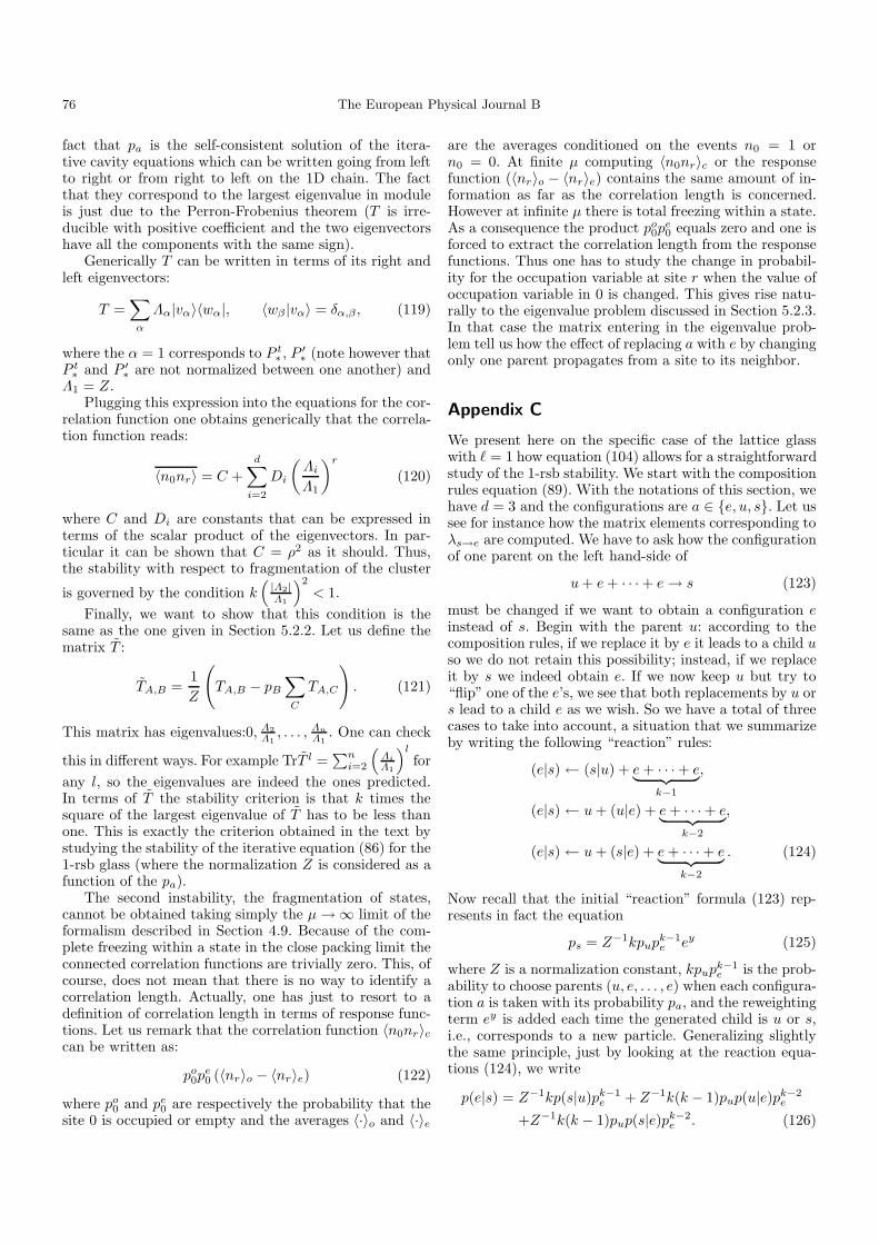
76 The European Physical Journal B
fact that pa is the self-consistent solution of the itera-tive cavity equations which can be written going from leftto right or from right to left on the 1D chain. The factthat they correspond to the largest eigenvalue in moduleis just due to the Perron-Frobenius theorem (T is irre-ducible with positive coefficient and the two eigenvectorshave all the components with the same sign).
Generically T can be written in terms of its right andleft eigenvectors:
T =∑α
Λα|vα〉〈wα|, 〈wβ |vα〉 = δα,β , (119)
where the α = 1 corresponds to P t∗ , P ′
∗ (note however thatP t∗ and P ′∗ are not normalized between one another) andΛ1 = Z.
Plugging this expression into the equations for the cor-relation function one obtains generically that the correla-tion function reads:
〈n0nr〉 = C +d∑
i=2
Di
(Λi
Λ1
)r
(120)
where C and Di are constants that can be expressed interms of the scalar product of the eigenvectors. In par-ticular it can be shown that C = ρ2 as it should. Thus,the stability with respect to fragmentation of the cluster
is governed by the condition k(
|Λ2|Λ1
)2
< 1.Finally, we want to show that this condition is the
same as the one given in Section 5.2.2. Let us define thematrix T :
TA,B =1Z
(TA,B − pB
∑C
TA,C
). (121)
This matrix has eigenvalues:0, Λ2Λ1, . . . , Λn
Λ1. One can check
this in different ways. For example TrT l =∑n
i=2
(Λi
Λ1
)l
forany l, so the eigenvalues are indeed the ones predicted.In terms of T the stability criterion is that k times thesquare of the largest eigenvalue of T has to be less thanone. This is exactly the criterion obtained in the text bystudying the stability of the iterative equation (86) for the1-rsb glass (where the normalization Z is considered as afunction of the pa).
The second instability, the fragmentation of states,cannot be obtained taking simply the µ→∞ limit of theformalism described in Section 4.9. Because of the com-plete freezing within a state in the close packing limit theconnected correlation functions are trivially zero. This, ofcourse, does not mean that there is no way to identify acorrelation length. Actually, one has just to resort to adefinition of correlation length in terms of response func-tions. Let us remark that the correlation function 〈n0nr〉ccan be written as:
po0p
e0 (〈nr〉o − 〈nr〉e) (122)
where po0 and pe
0 are respectively the probability that thesite 0 is occupied or empty and the averages 〈·〉o and 〈·〉e
are the averages conditioned on the events n0 = 1 orn0 = 0. At finite µ computing 〈n0nr〉c or the responsefunction (〈nr〉o − 〈nr〉e) contains the same amount of in-formation as far as the correlation length is concerned.However at infinite µ there is total freezing within a state.As a consequence the product po
0pe0 equals zero and one is
forced to extract the correlation length from the responsefunctions. Thus one has to study the change in probabil-ity for the occupation variable at site r when the value ofoccupation variable in 0 is changed. This gives rise natu-rally to the eigenvalue problem discussed in Section 5.2.3.In that case the matrix entering in the eigenvalue prob-lem tell us how the effect of replacing a with e by changingonly one parent propagates from a site to its neighbor.
Appendix C
We present here on the specific case of the lattice glasswith = 1 how equation (104) allows for a straightforwardstudy of the 1-rsb stability. We start with the compositionrules equation (89). With the notations of this section, wehave d = 3 and the configurations are a ∈ e, u, s. Let ussee for instance how the matrix elements corresponding toλs→e are computed. We have to ask how the configurationof one parent on the left hand-side of
u+ e+ · · ·+ e→ s (123)
must be changed if we want to obtain a configuration einstead of s. Begin with the parent u: according to thecomposition rules, if we replace it by e it leads to a child uso we do not retain this possibility; instead, if we replaceit by s we indeed obtain e. If we now keep u but try to“flip” one of the e’s, we see that both replacements by u ors lead to a child e as we wish. So we have a total of threecases to take into account, a situation that we summarizeby writing the following “reaction” rules:
(e|s) ← (s|u) + e+ · · ·+ e︸ ︷︷ ︸k−1
,
(e|s) ← u+ (u|e) + e+ · · ·+ e︸ ︷︷ ︸k−2
,
(e|s) ← u+ (s|e) + e+ · · ·+ e︸ ︷︷ ︸k−2
. (124)
Now recall that the initial “reaction” formula (123) rep-resents in fact the equation
ps = Z−1kpupk−1e ey (125)
where Z is a normalization constant, kpupk−1e is the prob-
ability to choose parents (u, e, . . . , e) when each configura-tion a is taken with its probability pa, and the reweightingterm ey is added each time the generated child is u or s,i.e., corresponds to a new particle. Generalizing slightlythe same principle, just by looking at the reaction equa-tions (124), we write
p(e|s) = Z−1kp(s|u)pk−1e + Z−1k(k − 1)pup(u|e)pk−2
e
+Z−1k(k − 1)pup(s|e)pk−2e . (126)

O. Rivoire et al.: Glass models on Bethe lattices 77
Here we put no reweighting since we generate an emptysite e. Using the equations for the pa, it can be simplifiedsomewhat, and when expressed with the λa→e defined byp(e|a) ≡ paλa→e, it becomes
λs→e = [λu→s + (k − 1)λe→u + (k − 1)λe→s]e−y. (127)
The five other equations are obtained by following thesame lines,
λu→e = kλe→se−y,
λu→s = kλe→u,
λs→u = λu→e,
λe→u = Z−1kpspk−2e λs→ee
y,
λe→s = Z−1kpspk−2e λs→ue
y+Z−1k(k − 1)p2up
k−3e λu→ee
y
+Z−1k(k − 1)pupspk−3e λs→ee
y. (128)
These six linear relations define the matrix T ; we thencompute its eigenvalue Λ2 as a function of y.
Appendix D
In this appendix we would like to show how the resultsobtained in the text with the cavity method can be re-produced with replicas. For an introduction to the replicamethod for random graphs with finite connectivity see forexample [20].
First, we introduce a function to encode in a compactway the conditional probability that the central site i for arooted sub-tree is empty (e), occupied but the constraintunsaturated (u) and finally occupied and the constraintsaturated (s), i.e., the root site has neighboring particles.We use the function f(τ) = C exp(hτ + gτ2) with τ =−1, 0, 1 where C, h, g are defined in such a way that
f(0) =Ξ
(e)i
Ξ(e)i +Ξ
(u)i +Ξ
(s)i
,
f(1) =Ξ
(s)i
Ξ(e)i +Ξ
(u)i +Ξ
(s)i
, (129)
f(−1) = 1− f(0)− f(1) =Ξ
(u)i
Ξ(e)i +Ξ
(u)i +Ξ
(s)i
.
The relation with the fields a, b can be easily established:
exp(−µa) =1
1 + exp(g − h) + exp(g + h), (130)
exp(−µb) =1
1 + exp(g − h). (131)
Now consider n replicated systems for the same ran-dom graph and define the function ψ(τ ):
ψ(τ ) = N⟨
n∏a=1
exp(h
(a)i τa + g
(a)i τ2
a
)⟩(132)
where the overline means the average over the disorder(or, analogously, one can average over sites for a fixedrandom graph), N is a normalization constant such that∑
τ ψ(τ ) = 1 and τ ≡ (τ1, . . . , τn).For the same reasons as discussed in the text in the
case of the cavity method, the grand potential per site isgiven by:
2ω = limn→0
1n
(−(k + 1)G(n)
edge + 2G(n)site
), (133)
G(n)edge = ln
∑τ ,τ ′
ψ(τ )ψ(τ ′)C(τ , τ ′), (134)
G(n)site = ln
∑τi,no
k+1∏i=1
ψ(τi)C(τi,n0) (135)
where C(τ , τ ′) and C(τi,n0) enforce the geometricalconstraint.
Differentiating ω with respect to ψ(τ ) we get the self-consistent equation
ψ(τ ) = N′∑
n0,τ i
k∏i=1
ψ(τi)C(τi,n0) (136)
where the prime over Σ means that, for each value of τ ,we sum only over those τi,n0 that give rise to τ .
Once the distribution ψ(τ ) is known all the observablescan be computed. For instance the density equals:
ρ = limn→0
1n
∑a,τi,no
nao
k+1∏i=1
ψ(τi)C(τi,n0). (137)
The most general replica symmetric solution can bewritten:
ψ(τ ) =∫dhdgP (h, g)
n∏a=1
exp(hτa + gτ2
a
)1 + exp(g + h) + exp(g − h)
(138)where P is a normalized probability distribution. Becauseof the homogeneity of the random graph with fixed con-nectivity, the rs solution is particularly simple,
P (h, g) = δ(h− hliq)δ(g − gliq). (139)
Using the relations (130–131) between h, g and a, b onecan rederive all the liquid properties (density, free energy,entropy, . . . ) obtained in the main part of the paper withthe cavity method.
Because of the homogeneity of the random graph, the1-rsb solution, in which replicas are divided in n/m groups(noted c) of m replicas each, also becomes simple andreads
ψ(τ ) =n/m∏c=1
∫dhdgP (h, g)
exp[∑
a∈c
(hτa + gτ2
a
)][1 + exp(g + h) + exp(g − h)]m
.
(140)

78 The European Physical Journal B
Plugging this expression into the general equation for ψ(τ )and changing variables from h, g to a, b we get back tothe equation on P (a, b), equation (43). Moreover usingthis 1-rsb expression of ψ(τ ) one can easily obtain allthe observables like the density, the free energy and thecomplexity.
References
1. D. Aldous, M. Steele, in Encyclopedia of MathematicalSciences, edited by H. Kesten (Springer, 2003), Vol. 110,pp. 1–72
2. R.J. Baxter, Annals of Combin. 3, 191 (1999)3. G. Biroli, M. Mezard, Phys. Rev. Lett. 88, 025501 (2002)4. J.-P. Bouchaud, L. Cugliandolo, J. Kurchan, M. Mezard,
in Spin Glasses and Random Fields, edited by A.P. Young(World Scientific, Singapore, 1998)
5. M.P. Ciamarra, M. Tarzia, A. de Candia, A. Coniglio,Phys. Rev. E 67, 057105 (2003)
6. S. Franz, M. Leone, J. Stat. Phys. 3-4, 535 (2003)7. T.C. Hales (1998), available at
http://www.math.pitt.edu/∼thales/PUBLICATIONS/
8. T. Kirkpatrick, D. Thirumalai, Phys. Rev. Lett. 58, 2091(1987)
9. T. Kirkpatrick, D. Thirumalai, Phys. Rev. B 36, 5388(1987)
10. T. Kirkpatrick, D. Thirumalai, P. Wolynes, Phys. Rev. A40, 1045 (1989)
11. T. Kirkpatrick, P. Wolynes, Phys. Rev. A 35, 3072 (1987)12. W. Kob, H.A. Andersen, Phys. Rev. E 48, 4364 (1993)13. F.R. Kschischang, B. Frey, H.-A. Loeliger, IEEE Trans.
Inform. Theory 47, 498 (2001)14. A. Lawlor et al., Phys. Rev. Lett. 89, 245503 (2002)15. M. Mezard, G. Parisi, Eur. Phys. J. B 20, 217 (2001)16. M. Mezard, G. Parisi, J. Stat. Phys. 111, 1 (2003)17. M. Mezard, G. Parisi, M.A. Virasoro, Spin-Glass Theory
and Beyond, Vol. 9 of Lecture Notes in Physics (WorldScientific, Singapore, 1987)
18. M. Mezard, G. Parisi, R. Zecchina, Science 297, 812 (2002)19. R. Monasson, Phys. Rev. Lett. 75, 2847 (1995)20. R. Monasson, J. Phys. A 31, 515 (1998)21. A. Montanari, M. Muller, M. Mezard, The Phase Diagram
of Random Heteropolymers (2003), cond-mat/030704022. A. Montanari, F. Ricci-Tersenghi, Eur. Phys. J. B 33, 339
(2003)23. F. Ritort, P. Sollich, Adv. Phys. 52, 219 (2003)24. L.K. Runnels, J. Math. Phys. 8, 2081 (1967)25. L.C.E. Struik, Physical aging in amorphous polymers and
other materials (Elsevier, Houston, 1978)26. G. Szipiro, Nature 424, 12 (2003)27. C. Toninelli, G. Biroli, D.S. Fisher (2003),
cond-mat/0306746
28. M. Weigt, A.K. Hartmann, Phys. Rev. E 63, 056127 (2001)29. M. Weigt, A.K. Hartmann, Europhys. Lett. 62, 533 (2003)30. J.S. Yedidia, W.F. Freeman, Y. Weiss, Technical report
TR-2002-35, Mitsubishi Electrical Research Laboratories(2002), available at http://www.merl.com