arX

iv:h

ep-p

h/97

0225

1v4

21

Nov

199

7

WM-97-103

September 14, 1997

Quark-Antiquark Bound States within aDyson-Schwinger Bethe-Salpeter Formalism

Cetin Savklıa,1, Frank Tabakinb,2

aDepartment of Physics, College of William and Mary, Williamsburg, Virginia 23185,

bDepartment of Physics & Astronomy, University of Pittsburgh, Pittsburgh,

Pennsylvania 15260

Abstract

Pion and kaon observables are calculated using a Dyson-Schwinger Bethe-Salpeterformalism. It is shown that an infrared finite gluon propagator can lead to quarkconfinement via generation of complex mass poles in quark propagators. Observ-ables, including electromagnetic form factors, are calculated entirely in Euclideanmetric for spacelike values of bound state momentum and final results are extrapo-lated to the physical region.

PACS codes: 12.39.-x, 11.10St, 13.40.Gp

Keywords: quark model, bound sates, confinement, mesons

1E-mail: csavkli@physics.wm.edu2E-mail: frankt@tabakin.phyast.pitt.edu

1 Introduction

Description of simple hadrons in terms of quark-gluon degrees of freedom has long been

an active area in physics. With the advent of TJNAF, which will be operating at inter-

mediate energies and therefore probing the structure of hadrons, there is new motivation

and need for a simple theoretical description of quark interactions. In this context, the

Dyson-Schwinger Bethe-Salpeter(DSBS) equation formalism has gained popularity in re-

cent years.3 The DSBS formalism serves to bridge the gap between nonrelativistic quark

models and more rigorous approaches, such as lattice gauge theory.

The main features of QCD can be summarized as chiral symmetry breaking, confine-

ment and asymptotic freedom. It is possible to address all of these features within the

DSBS formalism. In this formalism, the input is an effective gluon propagator which is

assumed to represent the interactions between quarks at all momentum transfers. The

choice of a vector interaction between quarks is motivated only by the desire to make a

connection with QCD degrees of freedom. In fact, whether a scalar or a vector interaction

should be used between quarks is a topic of debate not addressed in this paper.

While various applications of the DSBS formalism to pseudoscalar and vector mesons

have produced promising results, there are still some questions to be investigated. In this

paper, we address three issues. These are: a) Can an infrared gluon propagator lead

to confined quarks? b) The question of using Euclidean metric and extrapolation. c)

Dressing of the quark-gluon vertex in the DSBS equations while maintaining the chiral

limit ?

The organization of this paper is as follows: In section 2, the model is introduced

and the realization of the chiral limit, within the dressing scheme used in this paper, is

discussed. In section 3, the quark propagator functions obtained by solving the Dyson-

Schwinger equation are presented and the quark propagator is shown to be free of real

timelike poles, indicating that quarks can not be free, which is an implication and require-

ment of confinement. In section 4, meson and kaon observables, which are calculated using

a Euclidean metric(rather than a Wick rotation that only effects the internal momenta),

are presented. Finally, results are summarized and our conclusions are presented in section

3See Ref. [1] for an extensive review.

1

ν

µνS S G

γ Γ

0

µ

= +

Figure 1: Quark Dyson-Schwinger equation is shown. Only one vertex is dressed toprevent double counting.

5.

2 THE MODEL

The mechanism of chiral symmetry breaking and recovery of massless pseudoscalar bound

states(pion, kaon) in the limit of massless fermions(quarks) was originally discovered in

the papers of Nambu-Jona-Lasinio(NJL) [2]. Nambu-Jona-Lasinio’s model originally de-

scribed relativistic nucleon interactions through local, four-nucleon couplings. It is the

same philosophy that is followed in the DSBS calculations, except that now nucleons

are replaced with quarks and the contact interaction is replaced by an effective gluon

exchange between quarks. The Dyson-Schwinger(DS) and the Bethe-Salpeter(BS) equa-

tions employed in this work are shown in Figures 1 and 2. The DS equation describes

the propagation of quarks in the presence of gluons. The BS equation describes the

quark-antiquark bound state, in which the DS quark propagator is used.

In Fig. 1, the thin lines represent the current quark propagators for each flavor f:

i S0f(p) =

[ i

/p − m0f

]

, (1)

while the thick lines correspond to the dressed quark propagators:

i Sf(p) =[ i

Af (p) /p − Bf (p)

]

. (2)

Here Af (p) is a dimensionless normalization factor and Bf(p) has the units of mass(MeV).

The problem of how to systematically dress DS and BS equations has recently been

addressed[3, 4]. Dressing of all vertices consistently is motivated by the desire to make

a closer connection with QCD. The structure of the Dyson-Schwinger equation, when

2

µνG

µνG

Γν

γµ

Γµ

γν

21

21 χχ χ= +

Figure 2: The Bethe-Salpeter equation is shown. Only one vertex is dressed each time.This is necessary to preserve the chiral limit, which follows from the similarity of the BSand the DS equations.

combined with the chiral limit requirement, strictly restricts the choice of kernel for the

Bethe-Salpeter equation. The chiral limit in NJL type models 4 is obtained due to the

similarity of the Dyson-Schwinger and Bethe-Salpeter equations in the limit of massless

current quarks. In this limit, the quark mass function B(p) and the Bethe-Salpeter wave-

function Φ(p) for pseudoscalar massless bound states satisfy the same equation(to be

shown below). Therefore, for any given set of parameters of the model gluon propaga-

tor Gµν , the solution of the Dyson-Schwinger equation automatically implies a massless

pseudoscalar bound state solution for the Bethe-Salpeter equation. In other words, in the

chiral limit the quark Dyson-Schwinger equation produces the appropriate mass function

B(p) such that the BS equation produces a massless pseudoscalar bound state.

In order to prevent double counting, only one of the vertices in the Dyson-Schwinger

equation(Fig. 1) is dressed as indicated by the solid circle. Therefore, to preserve the

similarity between the BS and the DS equations in the chiral limit, we dress only one of

the quark-gluon vertices in constructing the BS equation. In order to keep the Bethe-

Salpeter equation symmetric(to treat quarks equally), the kernel is divided into two pieces,

where in each piece an alternate vertex is dressed, and contribution of those terms is

averaged(See Fig. 2). While the dressing of only one of the quark-gluon vertices in the BS

kernel does not represent a complete dressing, since cases where both quark-gluon vertices

are simultaneously dressed are excluded, with the proper choice of vertex Γµ, one has a

subset of all diagrams that produce the correct chiral limit.

Having stated the general structure of the DS and BS equations used in this calcula-

4See Refs. [6, 7] for an extensive review of the NJL type models, and Refs. [8] for an extended versionof it.

3

tion, we now discuss the chiral limit, and the choice of the gluon propagator Gµν(q).

In terms of quark and gluon propagators, the DS equation is written as

Sf (p) = S0f(p) + i4

3Sf (p)[

∫ d4q

(2π)4Gµν(p − q) Γµ(p, q)Sf(q)γν ]S0f(p). (3)

Similarly, the Bethe-Salpeter equation [9] determining the BS vertex function(a truncated

wavefunction, see later) χP (k) is given by

χP (k) = i4

3

∫

d4q

(2π)4Gµν(q − k)

1

2

[

Γν(−k−,−q−) Sd(−q−) χP (q) Su(q+) γµ

+γν Sd(−q−) χP (q) Su(q+) Γµ(q+, k+)

]

, (4)

where the 4-vector q+ = Pη1 + q, q− = Pη2 − q, η1 + η2 = 1, and P is the bound state

4-momentum. The BS vertex function χP (k) and its conjugate χP (k) are related [10] by

χP (ik0, ~k) = γ0χ∗P (−ik0, ~k)γ0. (5)

The normalization condition of the BS vertex function is derivable from the BS equation

itself. [11] If the interaction does not depend on the total bound state momentum, the

normalization condition reduces to

2P µ = iNc

∫

d4q

(2π)4trD

[

χP (q)∂

∂Pµ

S(q+) χ(q) S(−q−)

+χP (q) S(q+) χ(q)∂

∂PµS(−q−)

]

(6)

As it is well known, the dressing of electromagnetic vertices, such as the photon-quark

vertex, is constrained by the Ward-Takahashi identity,

qµΓµ(p′, p) = S−1(p′) − S−1(p), (7)

which guarantees the conservation of electromagnetic current at the vertex. Similarly,

due to color current conservation, the dressed quark-gluon interaction vertex, Γµ(p, q),

satisfies the Slavnov-Taylor identity [14]

qµΓµ(p′, p)[1 + b(q2)] = [1 − B(q, p)]S−1(p′) − S−1(p)[1 − B(q, p)], (8)

4

where functions b(q2) and B(q, p) are related to “ghost fields.” Since the QCD ghost field

contributions to Eq. 8 are not well understood we neglect their contributions. When ghost

fields are neglected, b(q2) and B(q, p) = 0; the Slavnov-Taylor identity then reduces to

the Ward-Takahashi identity Eq. 7. The minimal vertex that satisfies this identity in this

limit has been given by Ball-Chiu [15] as:

ΓµBC(p′, p) =

A(p′) + A(p)

2γµ +

(p′ + p)µ

p′2 − p2

[A(p′) − A(p)

2( /p′ + /p) + B(p′) − B(p)

]

.(9)

It is clear that one can add any term to this vertex that satisfies

qµΓµ(p′, p) = 0. (10)

Curtis-Pennington [16] have proposed such an additional vertex term. Here, for simplicity,

we consider only the Ball-Chiu dressing.

2.1 The Chiral Limit

To determine what type of quark-gluon vertex is allowed within the approximation scheme

employed here, let us analyze the chiral limit of the DS and the BS equations. In the

chiral limit the current quark masses m0 and the bound state momentum P vanishes. In

this limit, taking the spinor trace of the Dyson-Schwinger equation 3, one obtains

B(p) =i

3

∫ d4k

(2π)4Gµν(p − k)

B(k)

A2(k)k2 − B2(k)tr

[

Γµ(p, k) (1 +A(k)

B(k)/k) γν

]

. (11)

For a pseudoscalar bound state, in the chiral limit the BS vertex function is given by

χP (k) ≡ iγ5ΦP (k), (12)

where ΦP (k) is a scalar function of the relative momentum k, and bound state momentum

P = 0. With this definition, the BS equation for the bound state wavefunction ΦP (k) is

obtained as

ΦP (k) =i

3

∫

d4q

(2π)4Gµν(q − k)

1

2tr

[

γ5 Γν(k, q) Sd(q) γ5ΦP (q) Su(q) γµ (13)

+γ5 γν Sd(q) γ5ΦP (q) Su(q) Γµ(q, k)

]

.

5

Commuting γ5 through propagators and noting that in the chiral limit,

Sd(−q)Su(q) = −1

A2(q)q2 − B2(q),

Eq. 13 can be rewritten as

ΦP (k) =i

3

∫

d4q

(2π)4Gµν(q − k)

ΦP (q)

A2(q)q2 − B2(q)

tr[

(Γµ(q, k) − γ5Γµ(k, q)γ5)γν

]

2(14)

To ensure that B(k) and ΦP (k) satisfy the same equation in the chiral limit, therefore

producing a massless pion, the following condition should be satisfied

tr[

Γµ(q, k) (1 +A(k)

B(k)/k) γν

]

=tr

[

(Γµ(q, k) + Γµ(k, q))γν ]

2(15)

Clearly, the commonly used bare quark gluon vertex, Γµ = γµ satisfies this condition.

Furthermore, the condition Eq. 15 is also satisfied by the following part of the Ball-Chiu

vertex

Γµ(p′, p) =A(p′) + A(p)

2γµ +

(p′ + p)µ

p′2 − p2

A(p′) − A(p)

2( /p′ + /p). (16)

The B(p′)−B(p) part of the Ball-Chiu vertex would have contributed to the lefthandside

of Eq. 15 while it does not contribute to the righthandside. The contribution of this term

is small compared to the sum of other two terms. Therefore, it is a good approximation to

drop this term. The vertex Eq. 16 enables us to preserve the chiral limit while including

the dominant part of the quark-gluon vertex dressing as suggested by the Ward-Takahashi

identity. This approximate form(Eq. 16) of the Ball-Chiu vertex is used for the quark-

gluon coupling in this work.

Since the functions B(k) and ΦP (k) satisfy the same equation in the chiral limit,

they are equal upto a proportionality constant. With the help of the BS normalization

condition 6 it is found [12, 13] that

ΦP (k) =1

fπB(k), (17)

where fπ is the pion decay constant.

In order to complete the description of the model, one needs to choose a model for the

gluon propagator Gµν(q). The choice of Gµν(q) has been discussed in various papers[17].

6

Usually, the ultraviolet(q → ∞) or asymptotic behavior of Gµν(q) is borrowed from

QCD calculations, while its infrared(q → 0) or confining behavior is given by a sharply

falling function such as 1/q4 or δ4(q), to incorporate confinement. The problem with 1/q4

behavior is that it is not an integrable singularity and one needs to introduce an infrared

cutoff. While the δ4(q) form does not have this problem, it is perhaps too simple a form

to represent the physics in the infrared region; this issue requires further study. In this

paper, we show that an infrared finite propagator can not be ruled out on the

basis of quark Dyson-Schwinger and Bethe-Salpeter equations. The model used

here is

Gµν(q) = (gµν −qµqν

q2) [ GIR + GUV], (18)

where the infrared(q → 0) behavior, GIR, is modeled by a finite term

GIR(q) = G e−q2/σ2

, (19)

while the asymptotic(q → ∞) form, GUV, is taken from perturbative QCD calculations

GUV(q) = 2π2 d

(q2 + σ2) ln(τ + q2/Λ2QCD)

, (20)

with d = 12/(33 − 2 Nf) = 49, where Nf = 3 is the number of flavors. The QCD scale

parameter ΛQCD, determined by fitting high energy experiments(Particle Data Group,

1990), is chosen to be 225 MeV. The constant τ ensures the positivity of the asymptotic

piece as q → 0, and results are not very sensitive to this parameter. The τ is chosen to

be τ = 3. The σ2 in the denominator of the UV piece is introduced to ensure that the

infrared piece is the dominant contribution at low energies. Similar forms for the dressed

gluon propagator have been used in the literature[18, 19, 20, 21] with considerable success

in preliminary applications of Dyson-Schwinger Equations to hadronic physics. Here, we

develop this approach using a dressed quark-gluon vertex while maintaining the chiral

limit, and show that quarks can be confined with an infrared finite interaction.

Aside from current quark masses, mu,d ≈ 6± 2 MeV and ms ≈ 150± 50 MeV [22], which

are also the input parameters of QCD, there are only two unconstrained parameters(G, σ)

to vary to predict the data. Parameters G = 1.9710−4MeV−2 and σ = 750 MeV are chosen

to give the optimum overall fit. We choose the current quark mass of the strange quark to

7

fine tune the kaon mass. The current quark masses used in the calculation are: mu,d = 3

MeV, and ms = 60 MeV. The ratio ms/mu is well within acceptable limits [22]. In the

next section, we discuss the solution of the quark Dyson-Schwinger equation.

3 QUARK PROPAGATORS AND CONFINEMENT

The numerical solution of the DS equation Eq. 3 is performed through iteration to find

the quark propagator functions A(p2) and B(p2) in Euclidean metric. The details of the

numerical methods are explained in the Appendix. Solutions for A(p2) and M(p2) ≡

10−6

10−4

10−2

100

102

104

106

108

p2(GeV

2)

1.00

1.10

1.20

1.30

1.40

A(p

2)

u,d quark s quark

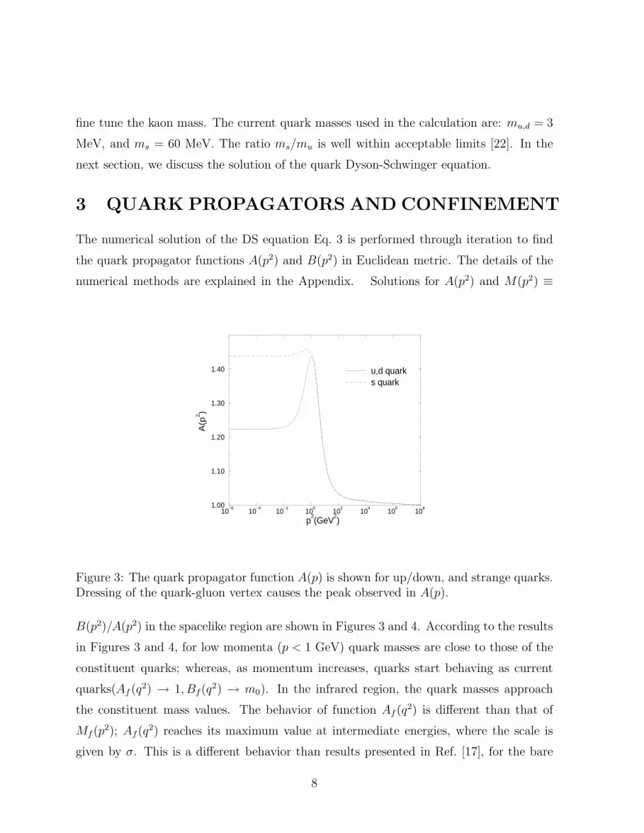
Figure 3: The quark propagator function A(p) is shown for up/down, and strange quarks.Dressing of the quark-gluon vertex causes the peak observed in A(p).

B(p2)/A(p2) in the spacelike region are shown in Figures 3 and 4. According to the results

in Figures 3 and 4, for low momenta (p < 1 GeV) quark masses are close to those of the

constituent quarks; whereas, as momentum increases, quarks start behaving as current

quarks(Af (q2) → 1, Bf(q2) → m0). In the infrared region, the quark masses approach

the constituent mass values. The behavior of function Af (q2) is different than that of

Mf (p2); Af (q

2) reaches its maximum value at intermediate energies, where the scale is

given by σ. This is a different behavior than results presented in Ref. [17], for the bare

8

10−6

10−4

10−2

100

102

104

106

108

p2(GeV

2)

−0.1

0.1

0.2

0.2

0.4

0.5

0.6

0.7

M(p

2)(

Ge

V)

u,d quark s quark

Figure 4: Quark mass functions M(p) are shown for up/down, and strange quarks. Atthe origin(p2 = 0), quark masses are closer to constituent quark mass values used innonrelativistic quark models. Asymptotically, quark mass values approach current quarkmass values.

quark-gluon coupling case. In their results, both M(p2) and Af(q2) are monotonically

decreasing functions. In our case, the dressing of the quark-gluon vertex gives rise to the

nonmonotonic behavior we found for Af (q2). As one increases the coupling strength G,

monotonic behavior of A is restored.

3.1 Test of Confinement

Confinement is the property that only color singlet hadrons are observed in nature. In

QCD, confinement is obtained dynamically due to the nonabelian, hence self-interacting,

nature of gluons. A natural result of confinement is that no free quark state should be

observed(a free quark state has a net color.) In QFT, an n-body bound state is defined

by the pole of the n-body propagator. The familiar 2-body(Bethe-Salpeter, Gross) and

3-body(Faddeev) equations are obtained, based on this definition, by looking for the poles

in the two and three body propagators. Similarly, it is natural to expect that a 1-body(or

free) state should be identified by the pole of the one body propagator. Therefore, if

9

quarks are confined, quark propagators should not have poles in the timelike(p2 > 0)

region.5, because such a pole permits an asymptotically(in space) free quark wave to

exist. The absence of poles in the quark propagators is, however, not conclusive evidence

for confinement. In order to be able to claim that a theory is confining, one has to also

show that a diquark, or any other color nonsinglet stable bound state does not exist.

Here, we restrict our discussion of confinement to quarks only. Therefore from here on,

“confinement” refers to “lack of free quarks” rather than the more general definition of

“lack of colored states.” In order to test whether a quark propagator, given in Euclidean

metric, leads to confinement, one needs a procedure to determine the presence of any poles

in the timelike region.6 For simple cases such as a free fermion, the Euclidean expression

for the propagator can be readily used to see if there are any poles when the propagator

is continued to the Minkowski metric, i.e.

1

p2E + m2

→1

p2 − m2, (21)

where there is a pole at p2 = m2. For the dressed quark propagator, the confinement test

question is: doesB(p2

E)

A2(p2E)p2

E + B2(p2E)

(22)

have a pole? For this test, the procedure used in Ref. [25] is adopted to determine whether

a quark propagator given in Euclidean metric has poles, when continued to Minkowski

metric. The starting point is the definition of a generalized quark propagator

S(p) ≡∫

dµ ρ(µ)i

/p − µ, (23)

where ρ(µ) is a spectral density function. The Euclidean metric expression for tr[SE(p)]

is

tr[SE(p)] = 4∫

dµ ρ(µ)µ

p2 + µ2. (24)

5There is an alternative to this approach, which is developed within the context of the Gross equationin Ref. [23]. In that approach, quarks are allowed to be on shell as long as they are in the vicinity ofoff-shell quarks, and confinement is realized through a relativistic generalization of the linear potential.

6An alternative realization of confinement can be obtained by simply defining the quark mass functionsuch that quark can never be on shell.[5] This approach amounts to having quark mass function M(p2)as input and the effective gluon propagator Gµν(q) as unknown in the quark Dyson-Schwinger equation.In this approach, a unique determination of the gluon propagator is not possible. Therefore, one is forcedto make a separable interaction approximation.

10

Using contour integration methods, the Fourier transform of this trace is found to be

∆(t) =∫

dp

2πeipt tr[SE(p)] (25)

= 2∫

dµ ρ(µ) e−µt . (26)

We define µ(t), the average effective mass(pole location) of the propagator S(p) as a

function of time by

µ(t) ≡ −∂

∂tln(∆(t)) (27)

=

∫

dµ ρ(µ) µ e−µt

∫

dµ ρ(µ) e−µt. (28)

Let us assume that S(p) has at least one pole for a finite p2 > 0. Let ρ(µ) =∑n−1

i=0 ci δ(µ−

mi), where n ≥ 1 and mi < mi+1. This assumption leads to a discrete average

µ(t) =

∑n−1i=0 ci mi e

−mit

∑n−1i=0 ci e−mit

. (29)

Taking the limit of this expression at infinite time t → ∞, one has

limt→∞

µ(t) ∼= m0. (30)

Therefore, this averaging procedure gives the smallest pole of the propagator S(p). If this

limit exists and it is real, then there is at least one finite pole for timelike momenta in the

Minkowski metric, and therefore the propagator does not represent a spatially confined

particle. On the other hand, if there is no finite limit or the limit is complex, then the

propagator represents a confined particle, since the propagator does not have a real finite

pole. This test for confinement has been applied to the quark propagator obtained from

the numerical solution of the Dyson-Schwinger equation. There are three possible pole

structures for the quark propagator. These possibilities are exemplified by the following:

• Real pole:

SE(pE) =1

p2E + m2

,

∆(t) ∝ e−mt,

µ(t) = m,

where the test produces the pole location as expected.

11

• Absence of poles:

SE(pE) = e−p2

E/(2σ2),

∆(t) ∝ e−σ2t2/2,

µ(t) = σt → ∞,

In this example, there is no finite pole and the propagator represents a confined particle.

This analytic form is the same as the infrared piece of the effective gluon propagator 19.

• Complex poles:

SE(pE) =1

(pE − ia)2 − m2,

Here the pole is complex in general and purely imaginary when a = 0. For this case, the

test results gives analytically

∆(t) ∝ e−atsin(mt),

µ(t) = a + m tan(mt −π

2).

Therefore, the signature of complex poles appears as M(t) ≡ µ(t) ∝ tan(mt) behavior as

t → ∞, where the frequency of oscillations is proportional to the imaginary part of the

quark mass pole. This is exactly the type of behavior found by applying the confinement

test to the quark propagator obtained by numerically solving the DS equation 3. Since

the quark propagator is known only numerically, application of the test is numerical

and details of the numerical methods are explained in the Appendix. Here we present

the test results for three different coupling strengths, namely G = 1 × 10−4, 1.5 × 10−4,

and 1.97 × 10−4MeV−2. The first case, G = 1 × 10−4MeV−2 is shown in Figure 5.

According to this result, the pole location is finite(≈ 110MeV) and real. Therefore,

this quark propagator does not represent a confined particle. On the other hand, this is

a case where the coupling constant is very small. As one increases the strength of the

coupling to G = 1.5 10−4MeV−2 an irregular oscillatory behavior sets in(Fig. 6). If the

coupling strength is further increased to G = 1.97 10−4MeV−2, which is the parameter

that is used to fit all observables in this paper, the oscillations clearly displays the

12

0.0 10.0 20.0 30.0 40.0 50.0time(200MeV/σ Fermi)

0.0

0.1

0.2

M(t

)(G

eV

)G=1.0 10

−4MeV

−2

Figure 5: Mass pole as a function of time is shown. Asymptotically, M(t) approaches aconstant, which indicates a real mass pole(unconfined quark).

tan(mt) behavior(Fig. 7) which indicates that quarks have complex mass poles.

According to this result(Fig. 7), the average distance a quark can travel before it

hadronizes, which is given by the average distance between the peaks(singularities) of the

M(t) function, is approximately D × 200MeV/σ Fermi = 1.45 × 200/750 = 0.39Fermi,

where D ≈ 1.45 is the average spacing between the peaks. This result is in very good

agreement when compared with the sizes of various hadronic bound states such as the

pion(rπ = .66 Fermi) and the kaon(rK = .53 Fermi). A recent study [24] of the DS

equation within the context of QED in three dimensions similarly finds complex conjugate

mass poles in the fermion propagator. It is important to emphasize that the analytic

form of the gluon propagator used in this calculation is not the only possible choice to

produce confined quarks. In fact, we have obtained similar results with other infrared

singular gluon propagators. Therefore, it is not possible to single out a specific analytic

form for the gluon propagator solely on the basis of the confinement test. Just as there

are infinitely many confining potentials in nonrelativistic quantum mechanics, there are

infinitely many confining effective gluon propagators in field theory. Therefore, additional

13

0.0 10.0 20.0 30.0 40.0 50.0time(200MeV/σ Fermi)

−50.0

−40.0

−30.0

−20.0

−10.0

0.0

10.0

20.0

30.0

40.0

50.0

M(t

)(G

eV

)G=1.5 10

−4MeV

−2

Figure 6: Mass pole as a function of time is shown. Oscillations indicate that quark masspole is complex.

0.0 10.0 20.0 30.0 40.0 50.0time(200MeV/σ Fermi)

−50.0

−40.0

−30.0

−20.0

−10.0

0.0

10.0

20.0

30.0

40.0

50.0

M(t

)(G

eV

)

G=1.97 10−4

MeV−2

Figure 7: As the strength of the coupling, G, is increased M(t) ∝ tan(t) behavior clearlysets in.

14

tests such as the prediction of meson observables are needed to determine if the gluon

propagator ansatz makes physical sense.

Having shown that it is possible to obtain confined quarks using a gluon propagator

with a gaussian type of infrared behavior, we now turn to the quark-antiquark bound

state problem.

4 QUARK-ANTIQUARK BOUND STATES

Before we embark on solving the BS equation, it is necessary to clarify a technical prob-

lem. In the previous section, dressed quark propagators were calculated in the Euclidean

metric(or spacelike momentum region). For the Bethe-Salpeter equation, usage of the

Euclidean metric is more problematic.7 Unlike the quark Dyson-Schwinger equation, the

Bethe-Salpeter equation involves the external total bound state momentum P , which has

to eventually represent a physical particle(bound state) with a real positive mass. There-

fore, the four momentum of the particle should be P = (m,~0), for which P 2 = m2 > 0

represents a timelike particle. It follows that, in order to be able to perform the inte-

grations in Eq. 4 in Euclidean metric, one needs to know the functions A(q2+), B(q2

+) for

q2+ = m2η1η2 − q2 + i mq0, where η1,2 is chosen to be

η1,2 =m1,2

m1 + m2

, (31)

and m1,2 ≡ Mu,d(0). On the other hand, functions A(q2+), B(q2

+) are known only for real

and spacelike q2+. The thick line in Fig. 8(the positive q2

+ axis) is where functions A(q2)

and B(q2) has been calculated by solving the Dyson-Schwinger equation. The domain

where these functions are needed is shown by the shaded region in Fig. 8. At this point,

there are three options. The first one, used in Ref. [28] among other works, is to assume

an analytic functional form that fits the numerical functions A(q2), B(q2) on the positive

real axis. Once this assumption is made one can use these analytic functions over the

entire complex plane. The second approach, which has been used in Ref. [18], is to Taylor

expand the functions A(q2), B(q2) around their real values to extend the results to the

complex plane. Both of these methods have drawbacks. It has been shown in previous

7Recent efforts to solve the BS equation directly in Minkowski metric are given in Refs. [26, 27]

15

m2

4

2q

q+2

Im

Re

plane

(0,0)

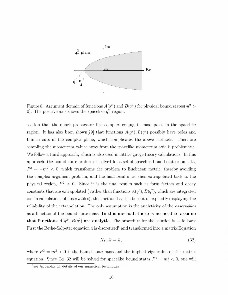
Figure 8: Argument domain of functions A(q2+) and B(q2

+) for physical bound states(m2 >0). The positive axis shows the spacelike q2

+ region.

section that the quark propagator has complex conjugate mass poles in the spacelike

region. It has also been shown[29] that functions A(q2), B(q2) possibly have poles and

branch cuts in the complex plane, which complicates the above methods. Therefore

sampling the momentum values away from the spacelike momentum axis is problematic.

We follow a third approach, which is also used in lattice gauge theory calculations. In this

approach, the bound state problem is solved for a set of spacelike bound state momenta,

P 2 = −m2 < 0, which transforms the problem to Euclidean metric, thereby avoiding

the complex argument problem, and the final results are then extrapolated back to the

physical region, P 2 > 0. Since it is the final results such as form factors and decay

constants that are extrapolated ( rather than functions A(q2), B(q2), which are integrated

out in calculations of observables), this method has the benefit of explicitly displaying the

reliability of the extrapolation. The only assumption is the analyticity of the observables

as a function of the bound state mass. In this method, there is no need to assume

that functions A(q2), B(q2) are analytic. The procedure for the solution is as follows:

First the Bethe-Salpeter equation 4 is discretized8 and transformed into a matrix Equation

HP 2 Φ = Φ, (32)

where P 2 = m2 > 0 is the bound state mass and the implicit eigenvalue of this matrix

equation. Since Eq. 32 will be solved for spacelike bound states P 2 = m2i < 0, one will

8see Appendix for details of our numerical techniques.

16

not be able to find any solutions unless an artificial eigenvalue αi is introduced to Eq. 32

Hm2

i

Φ = αiΦ. (33)

One proceeds by finding a set of solutions {m2i < 0, αi} to the above equation. This is

done by using an inverse iteration technique as explained in the Appendix. Using the set

of solutions {m2i < 0, αi}, a functional relationship between αi and m2

i can be established

αi = f(m2i ). (34)

It is only when m2i = m2 > 0 and αi = 1 that one recovers the original BS equation(32).

Therefore, location of the m2 that gives α = 1 is the eigenvalue and mass of the physical

bound state in question. The most general form for the spin-space part of the BS vertex

function for pseudoscalar mesons is given by

χP (k) = iγ5[Φ0 + /P Φ1 + /k Φ2 + [ /k, /P ] Φ3]. (35)

In the pseudoscalar meson channel, the dominant contribution to the BS vertex function

comes from the first term [18, 19],

χP (k) ≈ iγ5ΦP (k) (36)

This dominance is not surprising since the Dirac structure of the leading term in 36 is the

same as that of pointlike pion-quark coupling. Therefore, we only consider the leading

term in our analysis.9 The angular dependence of the BS vertex function is made explicit

by expanding it in terms of Tchebyshev polynomials

ΦP (k) =∞∑

n=0

ΦnP (|k|)T n(cosγ). (37)

For the bound states considered in this work(π, π∗, K±), the dominant contribution to

ΦP (k) comes from the T0 polynomial. Test runs for cases where higher(n > 0) Tcheby-

shev polynomials are included showed that the contribution of the higher Tchebyshev

polynomials are negligible, which is in agreement with conclusions in Ref. [18]. After

9For vector mesons, the leading term might not be the only important one.

17

−0.35 −0.25 −0.15 −0.05 0.05 0.15P

2(GeV

2)

0.6

0.8

1.0

1.2

α(P

2)

Eigenvalue α(P2)

2pim

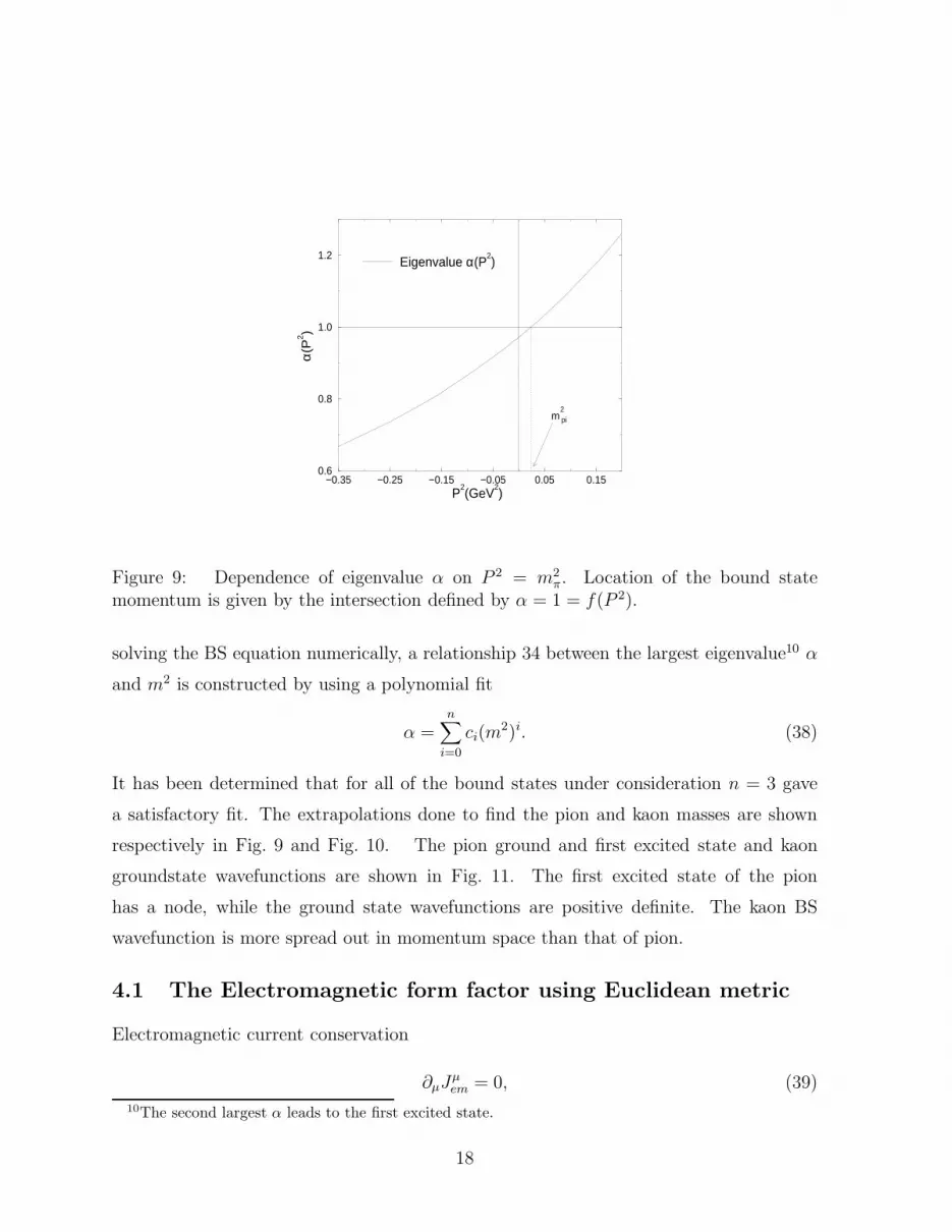
Figure 9: Dependence of eigenvalue α on P 2 = m2π. Location of the bound state

momentum is given by the intersection defined by α = 1 = f(P 2).

solving the BS equation numerically, a relationship 34 between the largest eigenvalue10 α

and m2 is constructed by using a polynomial fit

α =n

∑

i=0

ci(m2)i. (38)

It has been determined that for all of the bound states under consideration n = 3 gave

a satisfactory fit. The extrapolations done to find the pion and kaon masses are shown

respectively in Fig. 9 and Fig. 10. The pion ground and first excited state and kaon

groundstate wavefunctions are shown in Fig. 11. The first excited state of the pion

has a node, while the ground state wavefunctions are positive definite. The kaon BS

wavefunction is more spread out in momentum space than that of pion.

4.1 The Electromagnetic form factor using Euclidean metric

Electromagnetic current conservation

∂µJµem = 0, (39)

10The second largest α leads to the first excited state.

18

−1.4 −1.2 −1.0 −0.8 −0.6 −0.4 −0.2 0.0 0.2 0.4P

2(GeV

2)

0.2

0.6

1.0α

(P2)

Eigenvalue α(P2)

mK

2

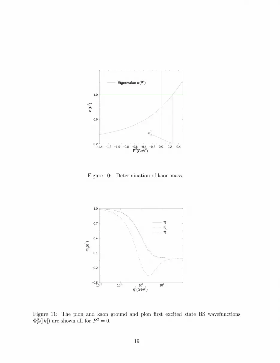
Figure 10: Determination of kaon mass.

10−2

10−1

100

101

q2(GeV

2)

−0.5

−0.2

0.1

0.4

0.7

1.0

Φ0(

q2)

πKπ∗

Figure 11: The pion and kaon ground and pion first excited state BS wavefunctionsΦ0

P (|k|) are shown all for P 2 = 0.

19

p+qp

Γµ

χ χπ π+ +

photon

uup/2+k p/2+k+q

q

p/2-k

d

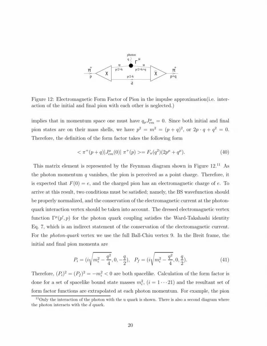
Figure 12: Electromagnetic Form Factor of Pion in the impulse approximation(i.e. inter-action of the initial and final pion with each other is neglected.)

implies that in momentum space one must have qµJµem = 0. Since both initial and final

pion states are on their mass shells, we have p2 = m2 = (p + q)2, or 2p · q + q2 = 0.

Therefore, the definition of the form factor takes the following form

< π+(p + q)|Jµem(0)| π+(p) >= Fπ(q2)(2pµ + qµ). (40)

This matrix element is represented by the Feynman diagram shown in Figure 12.11 As

the photon momentum q vanishes, the pion is perceived as a point charge. Therefore, it

is expected that F (0) = e, and the charged pion has an electromagnetic charge of e. To

arrive at this result, two conditions must be satisfied; namely, the BS wavefunction should

be properly normalized, and the conservation of the electromagnetic current at the photon-

quark interaction vertex should be taken into account. The dressed electromagnetic vertex

function Γµ(p′, p) for the photon quark coupling satisfies the Ward-Takahashi identity

Eq. 7, which is an indirect statement of the conservation of the electromagnetic current.

For the photon-quark vertex we use the full Ball-Chiu vertex 9. In the Breit frame, the

initial and final pion momenta are

Pi = (i

√

m2i −

q2

4, 0,−

q

2), Pf = (i

√

m2i −

q2

4, 0,

q

2). (41)

Therefore, (Pi)2 = (Pf)

2 = −m2i < 0 are both spacelike. Calculation of the form factor is

done for a set of spacelike bound state masses m2i , (i = 1 · · ·21) and the resultant set of

form factor functions are extrapolated at each photon momentum. For example, the pion

11Only the interaction of the photon with the u quark is shown. There is also a second diagram wherethe photon interacts with the d quark.

20

−6.4 −5.6 −4.8 −4.0 −3.2 −2.4 −1.6 −0.8 0.0P

2 (GeV

2)

0.50

0.60

0.70

0.80

0.90

F(P

2,q

i2)

q2=0.085 GeV

2

q2=.16 GeV

2

q2=.275 geV

2 m2

pi

calculated

extrapolated

For photon energies:

Figure 13: These plots show how the form factor extrapolation is done for various photonenergies. The extrapolated results are on the right hand side(timelike, P 2 = m2

π > 0) ofbound state momentum axis.

form factor at photon momentum of q2i is

F (m2, q2i ) =

n∑

j=0

Cj(q2i ) m2j , (42)

where Cj(q2i ) are the coefficients of a fit to the numerical result for F for photon momen-

tum of q2i . Therefore, the physical result for the pion form factor at the photon momentum

q2i is F (M2

π , q2i ). In Figure 13, we show the extrapolation for three different photon mo-

menta, q2 = 0.085 GeV2, q2 = 0.16 GeV2, and q2 = 0.275 GeV2. For each case, the result

of extrapolation is given by the value of the form factor functions at P 2 = m2π. In order

to ensure the reliability of the fit, a large number(21) of form factor calculations at each

photon momentum has been performed. The order of the polynomial fit used is n = 7.

According to the extrapolation results(Fig. 13) as the photon momentum increases, the

reliability of the extrapolation decreases. This difficulty is common to all solution meth-

ods(within the covariant DS-BS formalism) which use Euclidean metric.12 The reason for

12See Refs. [32] for a discussion of the transition to asymptotic(large q2) behavior of the pion formfactor within a light-cone Bethe-Salpeter formalism.

21

0.00 0.10 0.20 0.30 0.40q

2(GeV

2)

0.40

0.50

0.60

0.70

0.80

0.90

F(q

2)

ResultData

Figure 14: Extrapolated result for electromagnetic pion form factor.

this sensitivity is the increase in the curvature of the function F (m2, q2i ) with increasing

q2i . We present the form factor calculation for pion(Fig. 14) and kaon(Fig. 15) cases in

the region where the extrapolation is reliable. The data points for the pion form factor

are taken from Refs. [33, 34]. Data available from earlier experiments [35, 36] for the kaon

form factor are very poor. Experiments at TJNAF will hopefully provide better measure-

ments for both pion and kaon form factors. The pion decay constant, fπ, is defined by

the vacuum to one pion matrix element of the axial vector current:

< 0|J i5µ(x)| πj(p) >≡ ifπδijpµe

−ip·x. (43)

For a π+ meson at x = 0, this definition becomes:

< 0|Ψd(0)γµγ5λ−

2Ψu(0)|π+(p) >≡ ifπpµ. (44)

This matrix element corresponds to the Feynman diagram shown in Figure 16. Calculation

of decay constants are done using the same type of extrapolation technique used in the

calculations of masses and form factors. Values found are fK = 90.3(113) MeV, and fπ =

77.2(92.4) MeV, where numbers in parenthesis are the experimental measurements. The

22

0.00 0.02 0.04 0.06 0.08 0.10q

2(GeV

2)

0.5

0.7

0.9

1.1

[F(q

2)]

2

ResultData

Figure 15: Electromagnetic form factor of Kaon.

γµγ5p

π W+

µ

νµ

p/2+k

p/2-k

+

+

χ(k)

Figure 16: Pion Decay

23

pχπ

photon

photonΓp/2+k

Γν

µ

0

p/2-k

Figure 17: Neutral Pion Decay.

ratio of decay constants fK/fπ = 1.17(1.22) is in good agreement with the experimental

value and comparable to those found in similar works. It is reported in Ref. [20] that

next to leading order terms of the vertex function 35 contribute significantly to the decay

constants. This is a possible explanation for the low values we find for the decay constants.

As a final application, the neutral pion decay to two photons, π → γ +γ is considered.

Neutral pion decay is of historical importance since it is associated with the axial anomaly.

The matrix element for π0 → γγ decay(Fig. 17) is

T (k1, k2) = −2iαem

πfπǫµνρσ

×εµ∗(k1) εν∗(k2) k1ρ k2σ M(k1, k2), (45)

Since final photons are on-shell, k2i = 0, and P 2 = (k1 + k2)

2 = 2 k1 · k2 = m2π. Therefore

the scalar function M(k1, k2) is only a function of the pion mass. The decay rate

Γπ0→γγ = (αem

πfπ

)2 m2π

16πM(m2

π), (46)

is experimentally measured as Γπ0→γγ = 7.74 ± 0.56 eV, which means

gπ0γγ ≡ M(m2π) = 0.504 ± 0.019. (47)

It has been shown in Ref. [28] that, in chiral limit, irrespective of the details of quark

propagators, as long as the photon-quark vertices are properly dressed to conserve the

electromagnetic current and the BS vertex function is properly normalized, gπ0γγ is an-

alytically found to be 0.5. When the mass of the pion is taken into account, we find

gπ0γγ = .43 which is close to the experimental value.

A summary of the observables we calculated is given in Table 1. Error bars in exper-

imental measurements are negligible unless indicated.

24

Observable Calculated Experimental

mπ( MeV) 148 139.6fπ( MeV) 77.2 92.4

< r2π >1/2( Fermi) .65 .66

gπ0γγ .43 .504m∗

π( MeV) 1245 1300± 100mK( MeV) 515 495fK(MeV) 90.3 113

< r2K >1/2( Fermi) .54 .53

fK/fπ 1.17 1.22rK/rπ 0.83 0.8

Table 1: Summary of results

5 CONCLUSION

In this work, we analyzed three aspects of the Dyson-Schwinger Bethe-Salpeter equation

approach. We have shown that it is possible to dress the quark-gluon vertex beyond

the simple γµ form while maintaining the chiral limit condition. We have shown that

an infrared finite gluon propagator can lead to confined quarks through generation of

complex quark masses. It was found that, according to the model presented here, quarks

can freely propagate only ≈ 0.4 Fermi which is in very good agreement with the hadronic

bound state sizes. We have calculated all observables, including the pion form factor,

using a Euclidean metric approach without relying on the analyticity properties of quark

propagator functions A(p2) and B(p2). It is found that the extrapolations associated with

the usage of Euclidean metric are reliable up to 1 GeV2 for calculation of masses, and up

to around .5GeV2 for the calculation of form factors.

6 ACKNOWLEDGMENTS

We gratefully acknowledge very useful and encouraging discussions with Dr. Craig Roberts.

Dr. Conrad Burden is gratefully acknowledged for his input. This research was supported,

in part by the U.S. National Science Foundation international Grant INT9021617. One

of us(C. S.) has been supported by an Andrew Mellon Predoctoral Fellowship at the

University of Pittsburgh, and by the DOE through grant No. DE-FG05-88ER40435. We

25

also acknowledge receipt of a grant of Pittsburgh Supercomputer Center computer time.

A Numerical methods

Solutions of integral equations are performed by first discretizing the integrals

∫

dq f(q) −→n

∑

i=1

wi f(qi), (48)

where wi are integration weights for grid points qi. In order to map the grid points and

weights from interval (−1, 1) to (0,∞) we use the arctangent mapping(Ref. [30, 31])

y(x) = Rmin +Rdtan(π

4(1 + x))

1 + Rd

Rmax−Rmin

tan(π4(1 + x))

, (49)

where

Rd =Rmed − Rmin

Rmax − Rmed(Rmax − Rmin). (50)

It follows that

y(−1) = Rmin, y(0) = Rmed, y(1) = Rmax. (51)

Therefore, one can safely control the range(Rmin, Rmax) and distribution(Rmed) of grid

points. With this discretization procedure, continuous integral equations are transformed

into nonsingular matrix equations.

A.1 Dyson-Schwinger Equation

The DS equation involves two unknown functions A,B which appear in two coupled

equations(Eq. 3). After discretizing the associated integrals, one has the following matrix

equations

B = µI + G1 F1,

A = I + G2 F2. (52)

A,B,F1, and F2 are n dimensional vectors where

F1(i) ≡ B(i)/(B(i)2q2i + A(i)2),

F2(i) ≡ A(i)/(B(i)2q2i + A(i)2),

26

and G1 and G2 are n × n matrices. Coupled equations(Eq. 52) are solved for A, B by

forward iteration. An arbitrary initial guess for functions(vectors) A and B is entered

on the right hand side and the resulting vectors are iteratively used for the same process

until a stable solution is achieved. Grid points in momentum space have been chosen

for momenta between Rmin = 0 MeV and Rmax = 105σ MeV where σ is the relevant

momentum scale of the problem. The median of the grid point distribution was Rmed = 5σ

MeV. This uneven distribution of grid points ensures that the concentration of grid points

for lower momenta, that is where the integrand is maximum, is higher. Due to the smooth

nature of A and B functions only 40 grid points sufficed to find stable solutions. The

number of iterations needed to find a stable result is around 20.

A.2 Bethe-Salpeter Equation: Inverse Iteration Method

Here we outline the inverse iteration method originally developed in Refs. [30, 31].

The BS equation can be brought into the following form

[HM2 − α]Φ = 0, (53)

One starts with an arbitrary vector χ0

χ0 =N

∑

i=1

ci Φi (54)

where Φi, i = 1..N , satisfy

[HM2 − ωi]Φi = 0, (55)

where ωi, i = 1..N are eigenvalues of the HM2 matrix. Next, an arbitrary first guess for

α is chosen. It should be emphasized that eigenvalues which are not equal to α have no

physical meaning, for they do not correspond to a solution of the BS equation(Eq. 53).

In order to see if the initial guess α corresponds to one of the eigenvalues ωi, we construct

the operator

K =1

HM2 − α. (56)

Operating K on state χ0 n times produces

χn = Kn χ0 =N

∑

i=1

ci

(ωi − α)nΦi. (57)

27

When the number of iterations n is sufficiently large(usually around ten), the dominant

contribution to χn comes from the eigenvector Φj whose eigenvalue ωj satisfies |ωj −α| <

|ωi − α| for all i = 1..j − 1, j + 1..N . Therefore,

χn ≈cj

(ωj − α)nΦj ,

χn+1 ≈1

ωj − αχn. (58)

Using the eigenvector χn, which is proportional to Φj , one can also find eigenvalue ωj by

ωj =χn†Hχn

χn†χn. (59)

If ωj is close enough to α, then one has a self consistent solution. This method has

the benefit of directly singling out the eigenvalue closest to the initial guess, rather than

finding the largest eigenvalue as in the case of straight forward iteration. There is only

one matrix inversion involved. Distribution of the grid points in momentum space is done

by the arctangent mapping, as in the solution of the Dyson-Schwinger equation. The

typical number of momentum space grid points used in order to obtain stable solutions is

around 40. For angular integrals, 20 grid points which are linearly distributed in interval

(0, π) proved satisfactory.

A.3 Confinement test

Since the test of confinement involves a highly oscillatory integral Eq. 26, we have used

a large number, 30,000, of linearly distributed grid points. The upper limit of the mo-

mentum space integral, which is highly convergent, is 400σ. These choices allow one to

calculate the fourier transform(Eq. 26) confidently within the timeframe shown in Fig-

ures 5,6, and 7.

References

[*] Research supported in part by the NSF.

[1] C. D. Roberts and A. G. Williams, Prog. Part. Nucl. Phys. 33 (1994) 477.

28

[2] Y. Nambu and G. Jona-Lasinio, Phys. Rev. 122, 345 (1960); Phys. Rev. 124 (1961)

246.

[3] H.J. Munczek, Phys. Rev. D 52 (1995) 4736.

[4] A. Bender C. D. Roberts and L. V. Smekal, Phys. Lett. B 380 (1996) 7.

[5] M. Buballa, S. Krewald, Phys. Lett. B294 (1992) 19.

[6] S.P.Klevansky, Rev. of Mod. Phys. 64 No.3 (1992) 649.

[7] S. Klimt M. Lutz U. Vogl and W. Weise, Nucl. Phys. A 516, (1990) 429; Nucl. Phys.

A 516 (1990) 469.

[8] L.S. Celenza, A. Pantziris, C.M. Shakin, J. Szweda, Phys. Rev. C 47 (1993) 2356; L.

S. Celenza, C. M. Shakin, Wei-Dong Sun, Annals of Phys. 241 (1995) 1.

[9] E. E. Salpeter, H. A. Bethe, Phys. Rev. 84 (1951) 1232.

[10] S. Mandelstam, Proc. Roy. Soc. A 233 (1955) 248.

[11] See Itzykson, C. and Zuber, J. Quantum Field Theory, (McGraw-Hill, Inc., 1980) for

example.

[12] R. Jackiw and K. Johnson, Phys. Rev. D 8 (1973) 2386.

[13] R. Delbourgo and M. D. Scadron, J. Phys. G 5 (1979) 1621.

[14] Marciano, W. and Pagels, H. Quantum Chromodynamics, Phys. Rep. 36 (1977) 137.

[15] J. S. Ball and T.W. Chiu, Phys. Rev. D 22 (1980) 2542.

[16] D. C. Curtis and M. R. Pennington, Phys. Rev. D 46, (1992) 2663.

[17] P. Jain and H.J. Munczek, Phys. Rev. D 46 (1992) 438.

[18] P. Jain and H.J. Munczek, Phys. Rev. D 48 (1993) 5403.

[19] J. Praschifka R. T. Cahill and C.D Roberts, Int. J. of Mod. Phys., A4 (1989) 4929.

29

[20] C.J. Burden, Lu Qian, C.D. Roberts, P.C. Tandy, nucl-th/9605027, (1996).

[21] P.C. Tandy, Prog. Part. Nucl. Phys., Vol. 36 (1996) 97.

[22] J. Gasser and H. Leutwyler, Physics Reports 87, No 3 (1982) 77.

[23] F. Gross and J. Milana, Phys. Rev. D 43 (1991) 2401; 45 (1992) 969; 50 (1994)

3332.

[24] T. W. Allen C. J. Burden, Phys. Rev. D 53 (1996) 5842.

[25] F. T. Hawes C. D. Roberts A. G. Williams, Phys. Rev D 49 (1994) 4683.

[26] K. Kusaka and A. G. Williams, Phys. Rev. D 51 (1995) 7026.

[27] F. T. Hawes K. Kusaka and A. G. Williams, hep-ph/9411238, (1994).

[28] C. D. Roberts, Nucl. Phys. A 605 (1996) 475.

[29] S.J. Stainsby R.T. Cahill, Phys. Lett. A 146 9, (1990) 467.

[30] D. Heddle Y. R. Kwon F. Tabakin, Comp. Phys. Comm. 38 (1985) 71.

[31] Y. R. Kwon F. Tabakin, Phys. Rev. C 18 (1978) 932.

[32] L. S. Kisslinger and S.W. Wang, Nucl. Phys. B 399 (1993) 63.

[33] S. R. Amendolia, et al., Nucl. Phys. B 277 (1986) 168.

[34] C. J. Bebek, et al., Phys. Rev D 17, No 7 (1978) 1693.

[35] E. B. Dally, et al., Phys. Rev. Lett. 45 (1980) 232.

[36] S. R. Amendolia, et al., Phys. Lett. B 178 (1986) 435.

30